Behavior of Laterally Loaded Shafts Constructed Behind the Face of a
Mechanically Stabilized Earth Block Wall
BY
Matthew Pierson
Submitted to the graduate degree program in Civil
Engineering and Graduate Faculty of the University of
Kansas in partial fulfillment of the requirements for the
degree of Master of Science
___________________ Chairperson
Committee Members ___________________
___________________
Date defended: ___________________
ii
The Thesis Committee for Matthew Pierson Certifies that
this is the approved Version of the following thesis:
Behavior of Laterally Loaded Shafts Constructed Behind the Face of a
Mechanically Stabilized Earth Block Wall
___________________ Chairperson
Committee Members ___________________
___________________
Date approved: ___________________
iii
List of Figures: 2.1 Cutaway of typical MSE wall 52.2 True MSE abutment 82.3 Mixed MSE abutment 83.1.1 A) Regional map, B) Local map, C) Site map 113.1.2 Proposed cross section of MSE wall and subsurface 123.2.1 Plan view of MSE test wall and shafts 133.2.2 Wall facing layout 143.2.3 Typical steel configuration 153.2.4 Extension of CMP concrete form 173.2.5 Backfilling operation 183.3.1 Pressure cell protection 213.3.2 Photo target locations 223.3.3 Screen shots taken from AutoCadd during analysis 233.3.4 Typical test setup for single shafts 243.3.5 Group test setup 244.1.1 Large sieve analysis results 274.1.2 Large direct shear results 284.1.3 Mohr’s circle at failure for 5, 10, and 20 psi confining pressure 294.2.1 Shaft B load and deflection vs. time 304.2.2 Shaft B peak, 2.5 minute, and residual load vs. deflection 314.2.3 Peak load vs. deflection for all single shafts 324.2.4 Load at 2.5 minutes vs. deflection for all single shafts 324.2.5 Residual load vs. displacement for all single shafts 334.2.6 Shaft BG2 peak, 2.5 minute, and residual load vs. deflection 344.2.7 Peak load vs. displacement for shafts two diameters from the facing 354.2.8 2.5 minute load vs. displacement for shafts two diameters from the facing 364.2.9 Residual load vs. displacement for shafts two diameters from the facing 364.2.10 Distance from back of wall vs. load a four deflections 374.3.1 Shaft A centerline deflections 394.3.2 Shaft A deflection in horizontal direction el. 17.7 feet 394.3.3 Shaft A incremental centerline vertical deflection of wall face 404.3.4 Shaft A incremental horizontal deflection el. 17.7 feet 404.3.5 Shaft B centerline deflections 414.3.6 Shaft B deflection in horizontal direction el. 17.7 feet 424.3.7 Shaft B incremental centerline vertical deflection of wall face 424.3.8 Shaft B incremental horizontal deflection el. 17.7 feet 434.3.9 Shaft BS centerline deflections 444.3.10 Shaft BS deflection in horizontal direction el. 17.7 feet 44

iv
List of Figures (cont.): 4.3.11 Shaft BS incremental centerline vertical deflection of wall face 454.3.12 Shaft BS incremental horizontal deflection el. 17.7 feet 454.3.13 Shaft C centerline deflections 464.3.14 Shaft C deflection in horizontal direction el. 18.4 feet 474.3.15 Shaft C incremental centerline vertical deflection of wall face 474.3.16 Shaft C incremental horizontal deflection el. 18.4 feet 484.3.17 Shaft D centerline deflections 494.3.18 Shaft D deflection in horizontal direction el. 17.7 feet 494.3.19 Shaft D incremental centerline vertical deflection of wall face 504.3.20 Shaft D incremental horizontal deflection el. 17.7 feet 504.3.21 Shaft BG2 centerline deflections 514.3.22 Shaft BG2 deflection in horizontal direction el. 17.7 feet 524.3.23 BG2 incremental centerline vertical deflection of wall face 524.3.24 Shafts BG2 incremental horizontal deflection el. 17.7 feet 534.3.25 Shafts BG incremental horizontal deflection el. 17.7 feet 534.3.26 Shafts BG2 and B incremental horizontal deflection at elevation 17.7 feet 544.3.27 Shaft BG1 centerline deflections 554.3.28 Shaft BG1 deflection in horizontal direction el. 17.7 feet 554.3.29 Shaft BG1 incremental centerline vertical deflection of wall face 564.3.30 Shaft BG3 centerline deflections 564.3.31 Shaft BG3 deflection in horizontal direction el. 17.7 feet 574.3.32 Shaft BG3 incremental centerline vertical deflection of wall face 574.3.33 Peak load vs. maximum wall deflection for all shafts 584.3.34 Residual load vs. maximum wall deflection for all shafts 584.4.1 Shaft A pressure cells, load, and deflection of the shaft 604.4.2 Shaft B pressure cells, load, and deflection of the shaft 614.4.3 Shaft BS pressure cells, load, and deflection of the shaft 624.4.4 Shaft BG2 pressure cells, load, and deflection of the shaft 634.4.5 Shaft BG3 pressure cells, load, and deflection of the shaft 634.4.6 Shaft C pressure cells, load, and deflection of the shaft 644.4.7 Shaft D pressure cells, load, and deflection of the shaft 644.5.1 Surface cracks due to caving on back of shaft 664.5.2 Diagonal surface cracks 664.5.3 Crack developed above the end of reinforcement during group test. 674.5.4 Exhumed geogrid between shafts BG1 and BG2 674.5.5 Strain geogrid layer at 18.7feet elevation between shafts BG1 and BG2 686.2.1 Final facing deflection of the group of test shafts noon 706.2.2 Final facing deflection of the group of test shafts afternoon 71
v
List of Figures (cont.): 6.2.3 Profile of final wall deflection for group of test shafts 716.2.4 Side view of group wall facing final deflection 726.3.1 Distance from back of wall vs. influence length 74 List of Tables: 3.3.1 Geogrid Instrumentation 204.2.1 Peak Load vs. Displacement for all Shafts 364.2.2 Residual Load vs. Displacements for all Shafts 36/754.3.1 Peak Load vs. Maximum Wall Deflection 594.3.2 Residual Load vs. Maximum Wall Deflection 59/756.3.1 Distance from Wall Facing vs. Allowable Lateral Load and Influence Length 74

vi
Acknowledgements:
I would like to extend a special thanks to all people that play an important role in
not only my studies and this thesis, but also in my life. This must begin with my advisor
Dr. Robert Parsons who, by allowing me to work on this project, has given me one of the
greatest opportunities of my life. I must thank Dr. Jie Han, who has also served as a great
resource for my studies, activities, and research. The University of Kansas, for the
outstanding support that they have provided for my education and research.
The Kansas Department of Transportation deserves special thanks, without them
none of this would have been possible. James Brennan, whose diligence in maintaining a
high level of expectation was invaluable. Peter Wiehe along with the entire KDOT
maintenance crew proved to be exceptional craftsmen, as well as very committed
employees.
I would like to thank Tensar International for the commitment of expertise,
materials, and man hours. I would like to especially thank Christina Vulova, Andy
Anderson, and Joe Kerrigan who I had personal contact with and proved to be true
professionals.
Dr. Dan Brown, and Robert Thompson from Dan Brown and Associates, as well
all of the people from Applied Foundation Testing deserve many thanks. They were
integral in planning, load testing, and analysis of the test shafts.
I owe my parents, Jay and Gayle Pierson the greatest praise and thanks. They
have given me the tools to be successful and the support to use them. My wife to be Toni
Bishop, whose guidance, understanding, and passion are just a few of the things for
which I am thankful.
vii
Abstract:
Current practice for designing laterally loaded columns that pass through an MSE
Wall involves isolating the column from the MSE mass and anchoring the column into
rock with a rock socket. A sizeable cost and time savings could be realized, while still
maintaining reliability, if a method were available to evaluate the lateral load capacity of
a column that is supported by the MSE mass with no rock socket.
This report describes the construction, instrumentation, and testing of eight
different 36” diameter columns solely supported by an MSE mass as well as a brief
discussion of the results and recommendations for future testing and analysis.
Instrumentation includes 24 pressure cells, 16 inclinometer locations, 112 strain gages, 20
tell tales, 84 photo measurements of the wall facing, and load cells and LVDTs associated
with lateral load and response.
1
Chapter One
Introduction
Mechanically stabilized earth (MSE) walls are an inexpensive and aesthetically
attractive means of retaining soil. While the design principles for MSE structures have
been accepted for several decades, space restrictions at MSE wall sites have led to new
demands on MSE wall structures for which there are no well developed design
procedures. The specific area of research addressed in this thesis is to develop estimates
of the capacity of MSE structures to resist additional lateral loads applied to the MSE
structure by concrete columns, commonly referred to as drilled shafts, constructed within
the MSE mass. Developing an effective understanding of the lateral load capacity of the
wall and shafts will be of significant value for designing structures with significant lateral
loads that must be constructed on top of MSE structures, such as sound walls. Current
design procedures are by necessity based on very conservative design assumptions due to
the lack of test data. The research described in this thesis addresses this lack of data
through full scale testing of drilled shafts constructed within a laterally loaded MSE wall
backfill.
Mechanically stabilized earth structures have been constructed since ancient
times, but only relatively recently, with the advent of many synthetic materials, has this
technology gained wide spread use as an alternative to traditional concrete retaining
walls. These MSE walls typically use a high-density polyethylene or steel reinforcement
material with patterns of various types to transfer the load of the soil from the active zone
behind the wall face to much more stable material further from the wall. The result is a
2
stable, reinforced soil mass that typically has a masonry block, panel or welded wire and
fabric facing to prevent raveling or erosion of soil at the face and to enhance the aesthetic
value of the wall.
MSE walls must be designed with appropriate resistance factors or factors of
safety for all the failure mechanisms of conventional retaining walls. In addition, MSE
walls must be designed for modes of failure unique to MSE walls. Failure of an MSE
wall can occur several ways: sliding of layers, pullout of the reinforcement, elongation or
breakage of the reinforcement, and bulging of the facing. The entire mass must be check
for external stability. As with conventional walls, sliding, overturning, bearing capacity,
and deep seated stability, must be checked. Settlement issues are less of a problem with
an MSE wall then with a traditional concrete retaining wall, but must still be within a
reasonable limit.
Construction of a block MSE wall can be done with personnel with less skill than
a conventional wall due to the type of construction. Items requiring special care include
making sure each block is level, and aligned with the next block before the next course of
blocks can be placed on top. The geogrid must be placed into tension in order to prevent
excessive wall movement to mobilize strength in the geogrid. .
A 20 foot tall, 140 foot long MSE block wall was built using the Mesa system
developed by Tensar International. The wall supports eight 36 inch diameter vertical
shafts four different distances from the back of the facing to the center of the shaft.
These shafts were then loaded toward the wall facing using a displacement control
method. During this test, load and shaft deflection and inclination were monitored as

3
well as pressure behind the wall facing, strain in the geogrid layers, and wall facing
deflection.
The rest of this document will describe previous work, and design procedures for
MSE walls. It will also discuss construction and instrumentation of the project leading
up to testing. The testing method and procedure as well as the results will be discussed in
one section. Conclusions from this work related to design and recommendations for
future testing will also be addressed.
4
Chapter 2
Literature Review
Currently there is little published guidance for designing laterally loaded shafts
supported within an MSE Wall. However there are complete design procedures for each
item individually. These will be reviewed, as well as two other research projects that
study the combined uses of MSE Walls to support bridge abutments.
2.1 MSE Wall Design (FHWA)
An MSE wall uses inclusions that are placed within a soil mass to help distribute
tensile loads and prevent slope failure. One type of MSE structure not discussed here,
Reinforced Soil Slopes (RSS), incorporate planar reinforcing elements in constructed
earth-sloped structures with face inclinations of less then 70 degrees
(FHWA, 1996). MSE Walls use the same planar reinforcing and typically require a
facing to retain the soil within the structure. “Some common facings include precast
concrete panels, dry cast modular blocks, metal sheets and plates, gabions, welded wire
mesh, shotcrete, wood lagging and panels, and wrapped sheets of geosynthetics”
(FHWA, 1996). Most MSE systems use either a galvanized or epoxy coated steel
reinforcement, or synthetic reinforcement like high density polyethylene (HDPE),
polypropylene, or polyester yarn. The wall system used for this project is called The
Mesa System developed by Tensar International (See Figure 2.1). It utilizes dry cast
modular blocks and HDPE reinforcement.
According to FHWA (FHWA, 1996) branches and other different types of
reinforcement have been used for at least 1000 years. Beginning in the early 1960’s
reinforced soils began to be used in engineering by the French architect and engineer
5
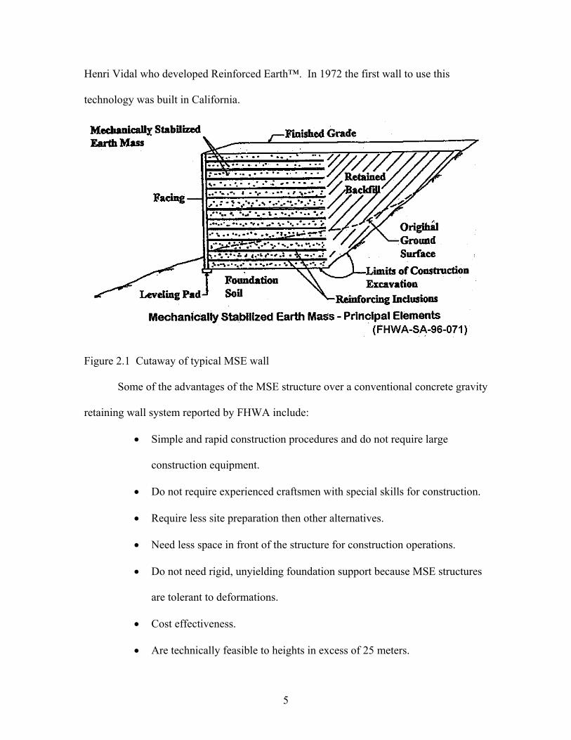
Henri Vidal who developed Reinforced Earth™. In 1972 the first wall to use this
technology was built in California.
Figure 2.1 Cutaway of typical MSE wall
Some of the advantages of the MSE structure over a conventional concrete gravity
retaining wall system reported by FHWA include:
• Simple and rapid construction procedures and do not require large
construction equipment.
• Do not require experienced craftsmen with special skills for construction.
• Require less site preparation then other alternatives.
• Need less space in front of the structure for construction operations.
• Do not need rigid, unyielding foundation support because MSE structures
are tolerant to deformations.
• Cost effectiveness.
• Are technically feasible to heights in excess of 25 meters.
6
When designing an MSE Wall structure there are several different failure modes
that must be checked. Design should consist of checking these modes of failure using
one or more of the following; working stress analysis, limit equilibrium analysis, and
deformation evaluations (FHWA). The first potential mode of failure is external stability.
This involves treating the entire reinforced mass as an internally stable block and
checking conventional failure modes for gravity wall systems. Possible failure
mechanisms include, sliding, overturning, bearing capacity, and deep seated stability.
Internal stability pertains to the reinforced soil mass. The reinforcement has two failure
types, elongation or breakage and reinforcement pullout. Bulging is a possibility
consisting of failure of the facing material. This could be a problem if the reinforcement
locations are not spaced close enough to prevent the lateral movement of individual
blocks. The step by step internal design process is as follows: (FHWA, 97)
• Select a reinforcement type
• Select the location of the critical failure surface.
• Select a reinforcement spacing compatible with the facing connections and to
prevent bulging.
• Calculate the maximum tensile force at each reinforcement level, static and
dynamic.
• Calculate the maximum tensile force at the connection to the facing.
• Calculate the pullout capacity at each reinforcement level.
Some additional issues may need to be addressed in design depending on the
situation. Traffic barriers are designed to take impact forces. Drainage should be
considered as well as the corrosion resistance of metal reinforcement. Utilities may need
7
to pass through the reinforced soil mass. Differential settlement with cast in place
structures must be considered. Surcharges as a result of road construction can increase
demand placed on the reinforcement. Rapid drawdown conditions may need to be
considered if tide or river fluctuations are possible. Obstructions in the reinforced soil
zone, such as drainage inlets, must be considered also.
2.2 Design of Laterally Loaded Shafts
When horizontal loads are being designed for drilled shafts the most common
method for analysis is the P-Y curve method. “This involves modeling the soil-structure
interaction as a nonlinear beam on elastic foundation. The model assumes that the soil is
continuous, isotropic, and elastic medium. The drilled shaft is divided into equally
spaced sections and the soil response is modeled by a series of closely spaced discrete
springs called Winkler’s springs” (Johnson, 2006). This model allows for the slope,
moment, shear, soil reaction, and deflection to be found for all sections along the drilled
shaft. The initial curves were found by doing full scale lateral load tests. The initial tests
were performed in soft and stiff clay, sand, loess, and limestone. These lateral load tests
are the most accurate, but also the most expensive way to find the soil structure P-Y
response. There are programs that are available (LPILE) to predict P-Y curves based on
shaft geometry and soil conditions. Using engineering judgment it is possible to take the
site materials and use computer programs to generate predicted P-Y curves without doing
expensive lateral load testing. However, there are currently no programs that will
account for shafts supported by an MSE wall. One assumption made in each program is
that soil is modeled as a homogeneous half space. For the MSE wall the soil is
8
homogeneous but has discrete strips of reinforcement with different properties within it,
and the mass is not a half space, it is a wall or slightly larger than a quarter space.
2.3 Topics related to MSE Wall interaction with Bridges
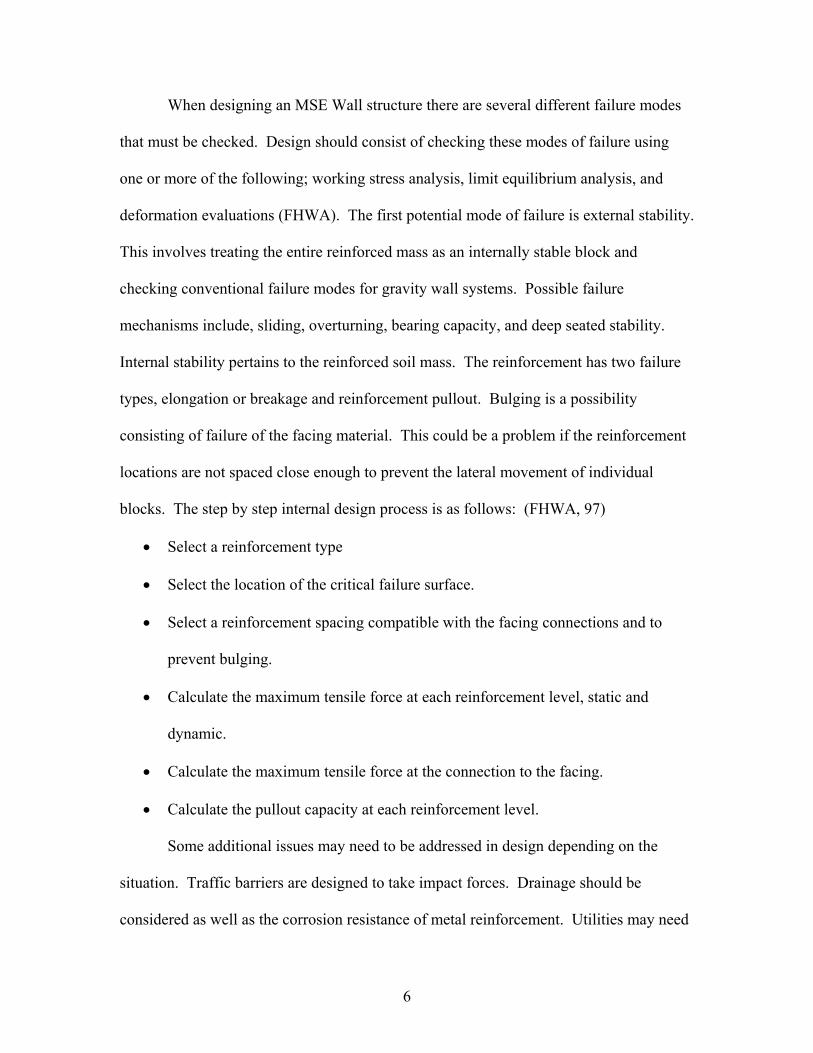
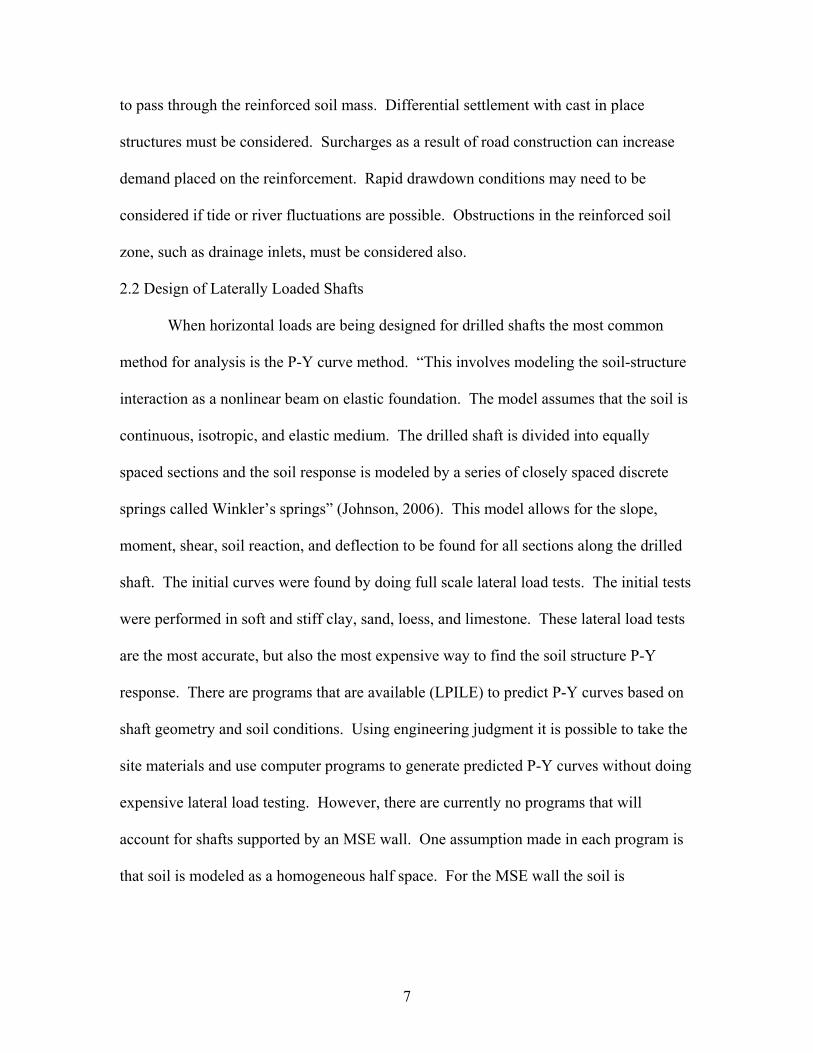
“There are two types of MSE abutments, true and mixed. In a true MSE
abutment the bridge load is placed directly on the MSE structure (See
Figure 2.2). To prevent overstressing the soil of a true abutment, the beam
seat is sized so the centerline of the bearing is at least 3 feet behind the
MSE wall face and the bearing pressure on the reinforced soil is no more
then four kips per square foot…A mixed abutment has piles or shafts
supporting the bridge seat (See Figure 2.3), with the MSE walls retaining
the fill beneath and adjacent to the end of the bridge. In some cases a
portion of the lateral load on the pile-supported seat is transmitted to the
MSE fill. This load can be resisted by MSE reinforcements in the wall or
by reinforcements extending from the back wall of the seat.” (Anderson,
2005)
Figure 2.2 True MSE abutment Figure 2.3 Mixed MSE abutment
9
For FHWA funded projects the design should follow FHWA details on the use of integral
abutments. There is no provision in the FHWA manual for shafts that are laterally
supported solely within an MSE Wall.
Constructability tests were performed on pile driving through HDPE geogrid
reinforced soil fill by Tensar International. A section of E-470 in Colorado contained
several mixed abutment type bridges. It was found that driving piles as close as four feet
from the facing caused no negative performance of the MSE structure. In addition to the
pile driving investigation one of the shafts was pushed over with a D9 bulldozer. It was
found that with three inches of pile movement only ¼” of facing movement occurred.
Clearly there are many areas of research that can be explored. The rest of this
document will describe the construction and testing of lateral load tests on shafts
constructed within an MSE fill in close proximity to the facing.

10
Chapter 3
Scope of Research
This chapter contains a description of the testing and initial analysis conducted in
association with this research. It includes a detailed discussion of the site investigation,
design, construction, instrumentation, and testing of the laterally loaded MSE test wall.
An accurate understanding of the load-deflection behavior is important for designing any
deep foundation for lateral loads. This behavior was monitored for eight shafts within an
MSE fill by conducting a series of full scale load tests. Also monitored during this time
was strain in four reinforcement layers, deformations within the fill using tell tales,
pressure at the face of the wall directly in front of each shaft at three elevations, and the
deflection of the facing at 82 points as a result of each loading step.
3.1 Site Investigation
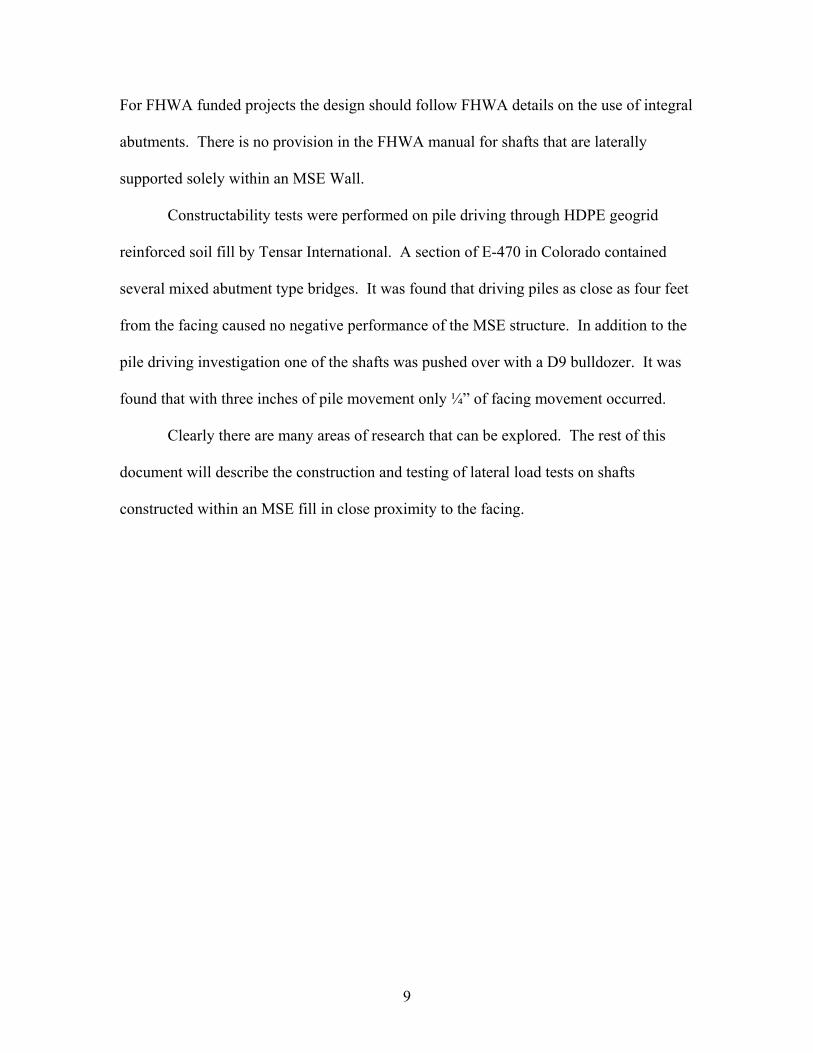
The site inside the southwest clover of the I-435/Leavenworth road interchange in
Kansas (Figure 3.1.1) was chosen for its access to a good limestone footing to found the
wall and the reaction shafts. All site investigation was performed by KDOT. Borings,
sampling, and in-situ testing were conducted. This was done to define the strata present
at the site in both elevation, and physical and mechanical properties, such as unconfined
compressive strength of the rock, or grain size distribution of the soil. The proposed
MSE wall and subsurface profile are shown in Figure 3.1.2. A typical boring log can be
found in the Appendix.
11
A) B)
C)
Figure 3.1.1 A) Regional map, B) Local map, C) Site map
12
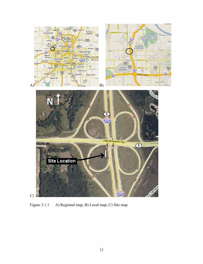
Figure 3.1.2 Proposed cross section of MSE wall and subsurface (KDOT, 2007)
3.2 Construction
A mechanically stabilized earth wall 140ft x 20ft was constructed using blocks
and geogrid provided by Tensar International. Eight test shafts 36” in diameter were
constructed at distances of one, two, three, and four diameters from the back of the wall.
One shaft was embedded 15 feet in the reinforced fill, all others were 20 feet. Three
identical shafts two diameters from the wall were tested as a group to determine if a
group effect was significant. The test shaft spacing was 15’, and the shaft layout is
shown in Figure 3.2.1. A reference section of wall without any shafts was also
constructed (see fig. 3.2.1). Six reaction shafts were rock socketed into limestone six feet
and 27’ behind the facing for use in loading the test shafts. The group reacted against
two 48” diameter shafts. Each remaining shaft had its own 36” diameter reaction shaft
except for D. Loading of D was accomplished by spanning the reaction shafts used to
test A and B (see fig 3.2.1).
13
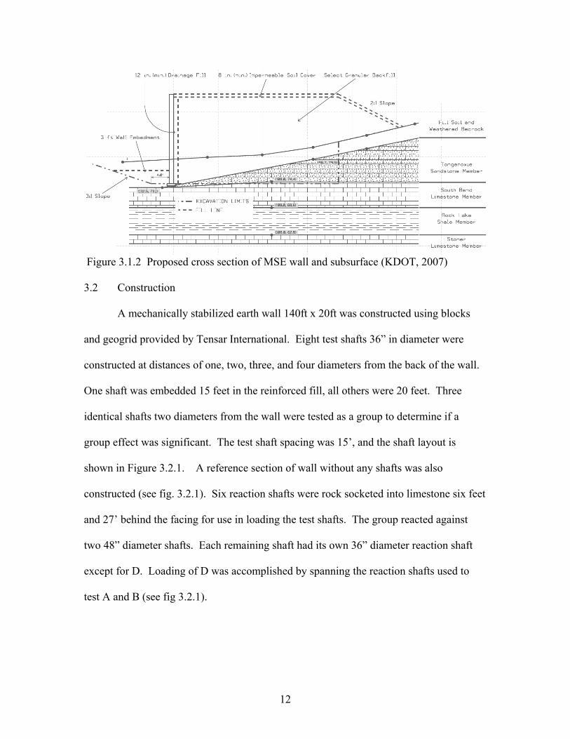
Tensar International, Inc. provided materials and technology from the Mesa
Retaining Wall System. This consisted of design, advising, Mesa units, welded wire
baskets, UX1400 and UX1500 geogrid, and connectors. Using a KDOT aggregate
Figure 3.2.1 Plan view of MSE test wall and shafts (Tensar, 2007)
specification for clean aggregate backfill (CA-5), it was decided to use a two foot spacing
(three blocks) for geogrid courses, and a geogrid length of 14’ (0.7 x H, H= height of
MSE Wall) from the facing. The UX1500 was used for the bottom four layers and
UX1400 was used for the top six. Wing walls with a welded wire basket design were
constructed at each end of the test wall. For the wing walls UX1400 was used at a 1.5’
spacing for the first four layers, and a three foot spacing for the top five layers of
14
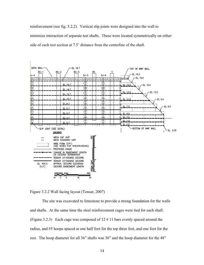
reinforcement (see fig. 3.2.2). Vertical slip joints were designed into the wall to
minimize interaction of separate test shafts. These were located symmetrically on either
side of each test section at 7.5’ distance from the centerline of the shaft.
Figure 3.2.2 Wall facing layout (Tensar, 2007)
The site was excavated to limestone to provide a strong foundation for the walls
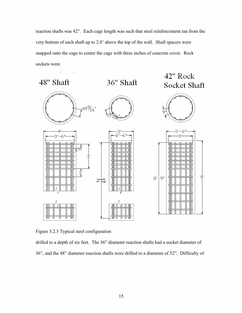
and shafts. At the same time the steel reinforcement cages were tied for each shaft.
(Figure 3.2.3) Each cage was composed of 12 # 11 bars evenly spaced around the
radius, and #5 hoops spaced at one half foot for the top three feet, and one foot for the
rest. The hoop diameter for all 36” shafts was 30” and the hoop diameter for the 48”
15
reaction shafts was 42”. Each cage length was such that steel reinforcement ran from the
very bottom of each shaft up to 2.8’ above the top of the wall. Shaft spacers were
snapped onto the cage to center the cage with three inches of concrete cover. Rock
sockets were
Figure 3.2.3 Typical steel configuration
drilled to a depth of six feet. The 36” diameter reaction shafts had a socket diameter of
36”, and the 48” diameter reaction shafts were drilled to a diameter of 52”. Difficulty of
16
extracting the rock from two holes lead to some over drilling with the deepest going one
foot over for a total depth of 7’. This resulted in adding some steel reinforcement to the
top of the shafts in order to maintain proper reinforcement.
Concrete for the drilled shafts was specified by KDOT to have a 9” slump and
that it was to be used for drilled shafts. The ready mix plant had an existing mix design
that was used. The results for slump and average compressive strength were 8 ½” and
6500psi respectively. For complete results see the Appendix.
Corrugated metal pipe (CMP) was used as a concrete form for the section of the
shafts contained within the crushed stone fill. The first sections were set using the hoist
truck, and legs were welded to the bottom of the CMP to maintain alignment. Next the
reinforcement cages were lowered into place, and plumbed using the hoist truck.
Concrete was then poured into the reaction shafts rock sockets and the first few feet of
the CMP. The hoist truck was left in place overnight to allow time for the concrete to
setup and hold the cages plumb.
Construction of a concrete leveling pad was required to serve as a base for the
Mesa block wall. This was two feet in width and had a minimum thickness of four inches
and a maximum thickness determined by the change in elevation of the limestone base
across the leveling pad. Number five bars were doweled into the limestone on either side
of the foundation to support the formwork. Concrete was placed and finished, and the
forms were left in place.
The CMP forms for the test shafts were set using the hoist truck and welded in
place to vertical dowels anchored in limestone. The CMP was positioned, plumbed and
then welded to the dowels for support for the first few feet of fill. As wall height
17
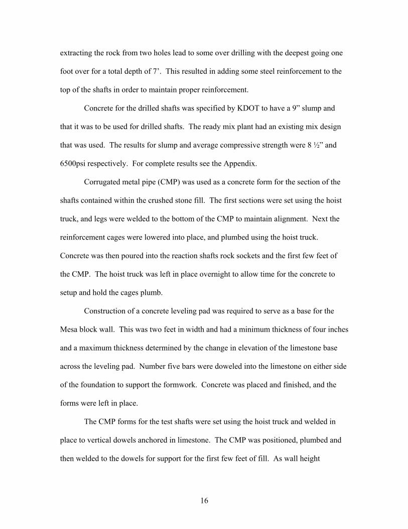
increased the upper section of CMP was added. This was done by first placing the CMP
with the hoist truck, and plumbing. The two CMP’s were then welded together, and a
band clamp was then tightened around the joint for added strength. The final height of
the CMP was cut off at 20’ of elevation. (Figure 3.2.4)
Figure 3.2.4 Extension of CMP concrete form
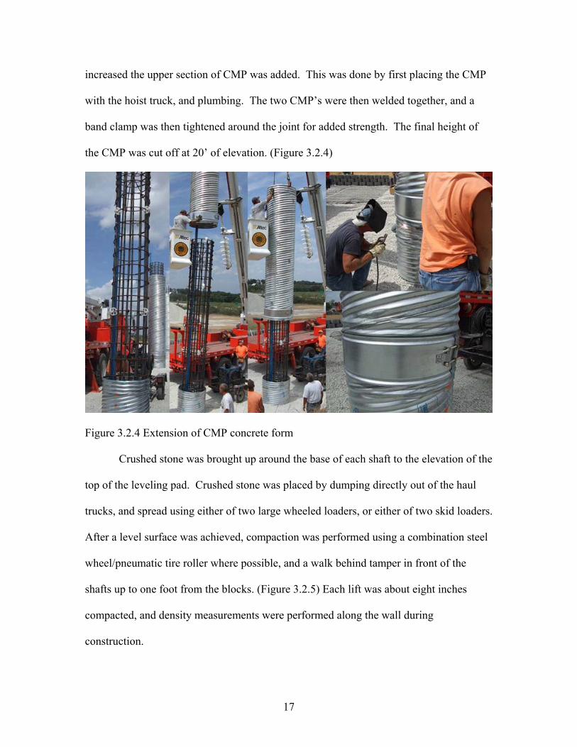
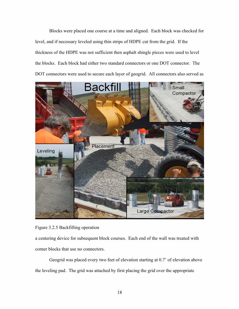
Crushed stone was brought up around the base of each shaft to the elevation of the
top of the leveling pad. Crushed stone was placed by dumping directly out of the haul
trucks, and spread using either of two large wheeled loaders, or either of two skid loaders.
After a level surface was achieved, compaction was performed using a combination steel
wheel/pneumatic tire roller where possible, and a walk behind tamper in front of the
shafts up to one foot from the blocks. (Figure 3.2.5) Each lift was about eight inches
compacted, and density measurements were performed along the wall during
construction.
18
Blocks were placed one course at a time and aligned. Each block was checked for
level, and if necessary leveled using thin strips of HDPE cut from the grid. If the
thickness of the HDPE was not sufficient then asphalt shingle pieces were used to level
the blocks. Each block had either two standard connectors or one DOT connector. The
DOT connectors were used to secure each layer of geogrid. All connectors also served as
Figure 3.2.5 Backfilling operation
a centering device for subsequent block courses. Each end of the wall was treated with
corner blocks that use no connectors.
Geogrid was placed every two feet of elevation starting at 0.7’ of elevation above
the leveling pad. The grid was attached by first placing the grid over the appropriate
19
block. The DOT connector was inserted through the grid and into the block with light
hammer blows. The grid was tensioned using pitch forks prior to completely driving.
Each subsequent course of blocks was then added aligned and leveled. Back
filling over geogrid was done by using a pitch fork to tension the grid and placing a small
amount of crushed stone over the end of the grid to hold it in tension. Additional fill was
then placed on tensioned grid. Crushed stone was spread while moving away from the
facing to ensure tension in the grid. Finally, compaction was carried out using the same
technique as the rest of the fill.
Slip joints were installed between each shaft to limit movement into neighboring
shafts. They were constructed by putting an end or corner treatment to the blocks. This
meant cutting every other block in the vertical direction and adding nonwoven geo-textile
matte to the middle of the slip joint.
In front of the wall 3.3’ of fill was placed to and lightly compacted. This fill was
soil from on site and consisted of broken up pieces of loosely cemented silty sand stone,
as well as top soil.
The top of the wall was capped with smaller architectural blocks. Crushed stone
fill was brought up to no greater then elevation 19.2’ and the final height of 20’ was
achieved using a low permeability soil cover. Each shaft was capped with a roughly
cubical block of concrete. These blocks were formed to be one inch wider then the shaft
each would cap. Concrete was added to each shaft to reach the final elevation 23’ above
the leveling pad.
20
3.3 Instrumentation
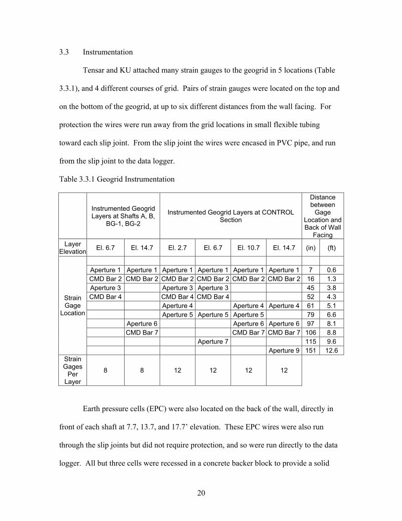
Tensar and KU attached many strain gauges to the geogrid in 5 locations (Table
3.3.1), and 4 different courses of grid. Pairs of strain gauges were located on the top and
on the bottom of the geogrid, at up to six different distances from the wall facing. For
protection the wires were run away from the grid locations in small flexible tubing
toward each slip joint. From the slip joint the wires were encased in PVC pipe, and run
from the slip joint to the data logger.
Table 3.3.1 Geogrid Instrumentation
Instrumented Geogrid Layers at Shafts A, B,
BG-1, BG-2
Instrumented Geogrid Layers at CONTROL Section
Distance between
Gage Location and Back of Wall
Facing Layer
Elevation El. 6.7 El. 14.7 El. 2.7 El. 6.7 El. 10.7 El. 14.7 (in) (ft)
Aperture 1 Aperture 1 Aperture 1 Aperture 1 Aperture 1 Aperture 1 7 0.6 CMD Bar 2 CMD Bar 2 CMD Bar 2 CMD Bar 2 CMD Bar 2 CMD Bar 2 16 1.3 Aperture 3 Aperture 3 Aperture 3 45 3.8 CMD Bar 4 CMD Bar 4 CMD Bar 4 52 4.3
Aperture 4 Aperture 4 Aperture 4 61 5.1 Aperture 5 Aperture 5 Aperture 5 79 6.6
Aperture 6 Aperture 6 Aperture 6 97 8.1 CMD Bar 7 CMD Bar 7 CMD Bar 7 106 8.8 Aperture 7 115 9.6
Strain Gage
Location
Aperture 9 151 12.6 Strain Gages
Per Layer
8 8 12 12 12 12
Earth pressure cells (EPC) were also located on the back of the wall, directly in
front of each shaft at 7.7, 13.7, and 17.7’ elevation. These EPC wires were also run
through the slip joints but did not require protection, and so were run directly to the data
logger. All but three cells were recessed in a concrete backer block to provide a solid
21
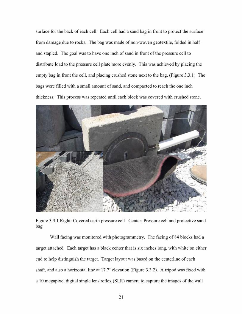
surface for the back of each cell. Each cell had a sand bag in front to protect the surface
from damage due to rocks. The bag was made of non-woven geotextile, folded in half
and stapled. The goal was to have one inch of sand in front of the pressure cell to
distribute load to the pressure cell plate more evenly. This was achieved by placing the
empty bag in front the cell, and placing crushed stone next to the bag. (Figure 3.3.1) The
bags were filled with a small amount of sand, and compacted to reach the one inch
thickness. This process was repeated until each block was covered with crushed stone.
Figure 3.3.1 Right: Covered earth pressure cell Center: Pressure cell and protective sand bag
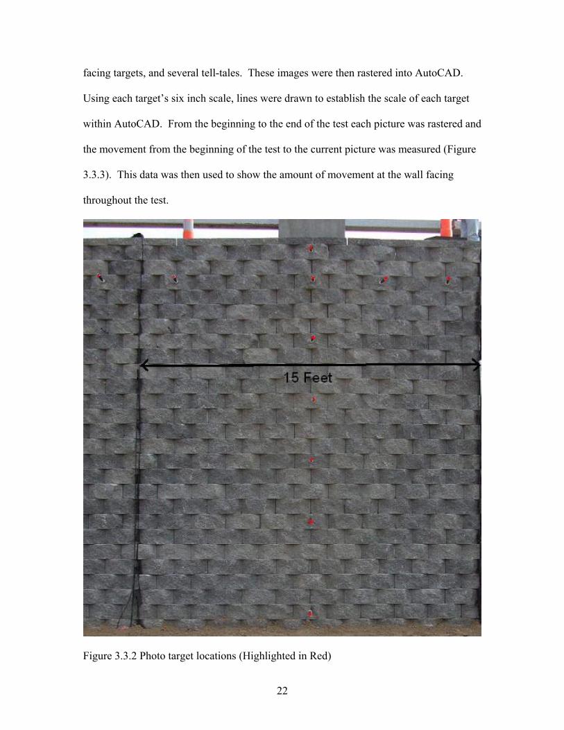
Wall facing was monitored with photogrammetry. The facing of 84 blocks had a
target attached. Each target has a black center that is six inches long, with white on either
end to help distinguish the target. Target layout was based on the centerline of each
shaft, and also a horizontal line at 17.7’ elevation (Figure 3.3.2). A tripod was fixed with
a 10 megapixel digital single lens reflex (SLR) camera to capture the images of the wall
22
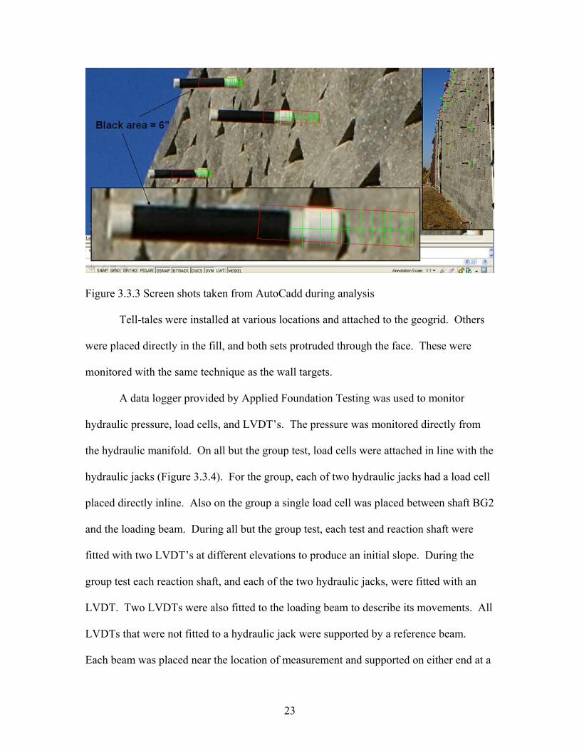
facing targets, and several tell-tales. These images were then rastered into AutoCAD.
Using each target’s six inch scale, lines were drawn to establish the scale of each target
within AutoCAD. From the beginning to the end of the test each picture was rastered and
the movement from the beginning of the test to the current picture was measured (Figure
3.3.3). This data was then used to show the amount of movement at the wall facing
throughout the test.
Figure 3.3.2 Photo target locations (Highlighted in Red)
23
Figure 3.3.3 Screen shots taken from AutoCadd during analysis
Tell-tales were installed at various locations and attached to the geogrid. Others
were placed directly in the fill, and both sets protruded through the face. These were
monitored with the same technique as the wall targets.
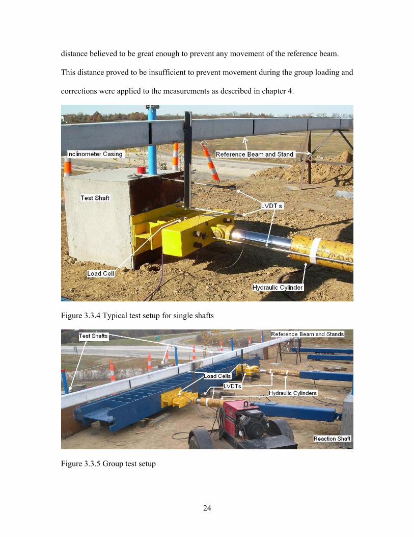
A data logger provided by Applied Foundation Testing was used to monitor
hydraulic pressure, load cells, and LVDT’s. The pressure was monitored directly from
the hydraulic manifold. On all but the group test, load cells were attached in line with the
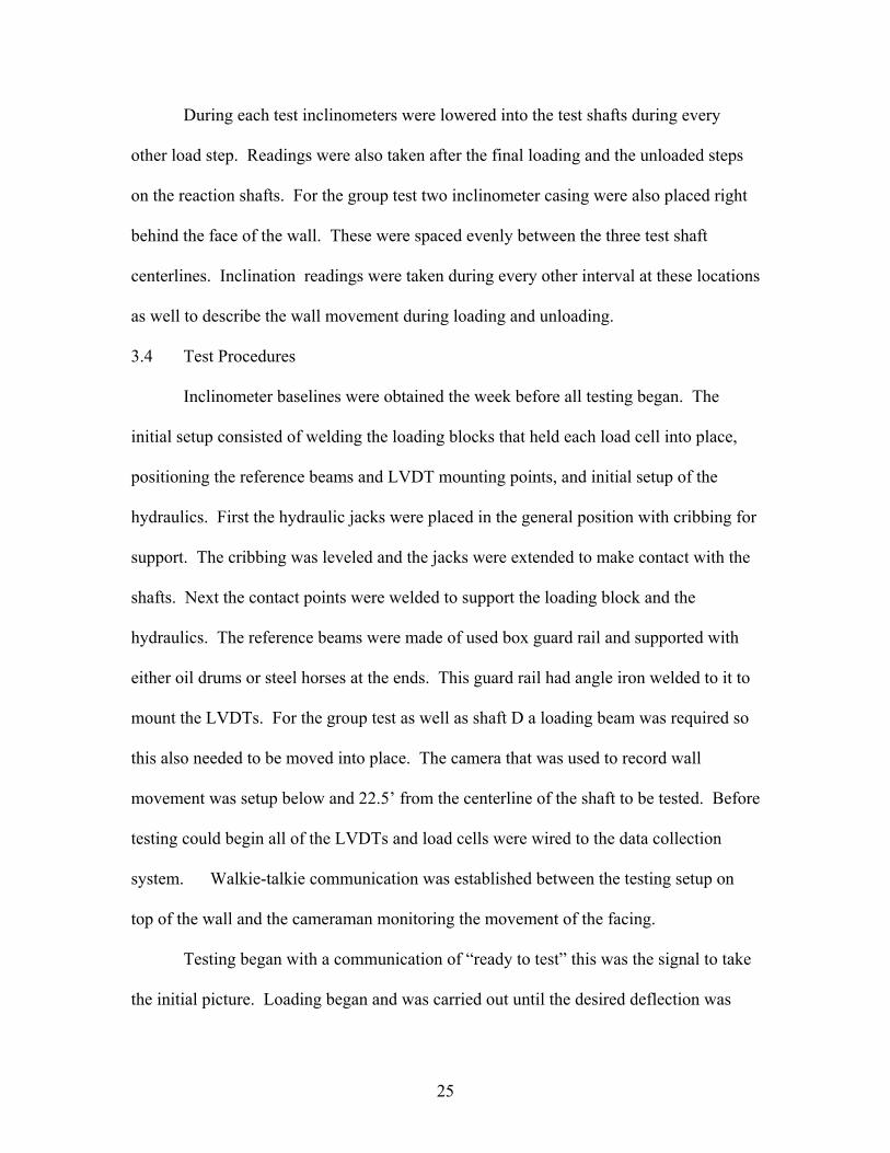
hydraulic jacks (Figure 3.3.4). For the group, each of two hydraulic jacks had a load cell
placed directly inline. Also on the group a single load cell was placed between shaft BG2
and the loading beam. During all but the group test, each test and reaction shaft were
fitted with two LVDT’s at different elevations to produce an initial slope. During the
group test each reaction shaft, and each of the two hydraulic jacks, were fitted with an
LVDT. Two LVDTs were also fitted to the loading beam to describe its movements. All
LVDTs that were not fitted to a hydraulic jack were supported by a reference beam.
Each beam was placed near the location of measurement and supported on either end at a
24
distance believed to be great enough to prevent any movement of the reference beam.
This distance proved to be insufficient to prevent movement during the group loading and
corrections were applied to the measurements as described in chapter 4.
Figure 3.3.4 Typical test setup for single shafts
Figure 3.3.5 Group test setup
25
During each test inclinometers were lowered into the test shafts during every
other load step. Readings were also taken after the final loading and the unloaded steps
on the reaction shafts. For the group test two inclinometer casing were also placed right
behind the face of the wall. These were spaced evenly between the three test shaft
centerlines. Inclination readings were taken during every other interval at these locations
as well to describe the wall movement during loading and unloading.
3.4 Test Procedures
Inclinometer baselines were obtained the week before all testing began. The
initial setup consisted of welding the loading blocks that held each load cell into place,
positioning the reference beams and LVDT mounting points, and initial setup of the
hydraulics. First the hydraulic jacks were placed in the general position with cribbing for
support. The cribbing was leveled and the jacks were extended to make contact with the
shafts. Next the contact points were welded to support the loading block and the
hydraulics. The reference beams were made of used box guard rail and supported with
either oil drums or steel horses at the ends. This guard rail had angle iron welded to it to
mount the LVDTs. For the group test as well as shaft D a loading beam was required so
this also needed to be moved into place. The camera that was used to record wall
movement was setup below and 22.5’ from the centerline of the shaft to be tested. Before
testing could begin all of the LVDTs and load cells were wired to the data collection
system. Walkie-talkie communication was established between the testing setup on
top of the wall and the cameraman monitoring the movement of the facing.
Testing began with a communication of “ready to test” this was the signal to take
the initial picture. Loading began and was carried out until the desired deflection was
26
achieved. At that point loading stopped and the hydraulic cylinders were locked into
position and held for five minutes or until inclinometer readings were finished. During
that time pictures were taken immediately after loading and then every 1.25 minutes until
it was time to load again. The loading procedure was repeated until the final loading
step. After the last load was applied and locked off, inclinometer readings were made on
all shafts or casing associated with that test, and then the entire setup was completely
unloaded. Finally another complete set of inclinometer readings were made at the
unloaded positions.
During construction, testing, and test analysis lab tests were run to obtain
properties of the CA-5 clean aggregate backfill. These tests consisted of sieve analyses,
triaxial compression tests, and large direct shear tests. The results of these tests are
contained in the next chapter.
27
Chapter 4
Test Results and Analysis
Results of the full scale lateral load testing, as well as laboratory tests used to
determine the properties of the aggregate backfill, are presented in this chapter. Results
of site investigation tests are presented in Appendix.
4.1 Laboratory Results and Analysis
The University of Kansas performed large direct shear, triaxial compression, and
sieve analysis tests on the Clean Aggregate backfill (CA-5). Samples were collected
from several different loads of aggregate during construction of the wall.
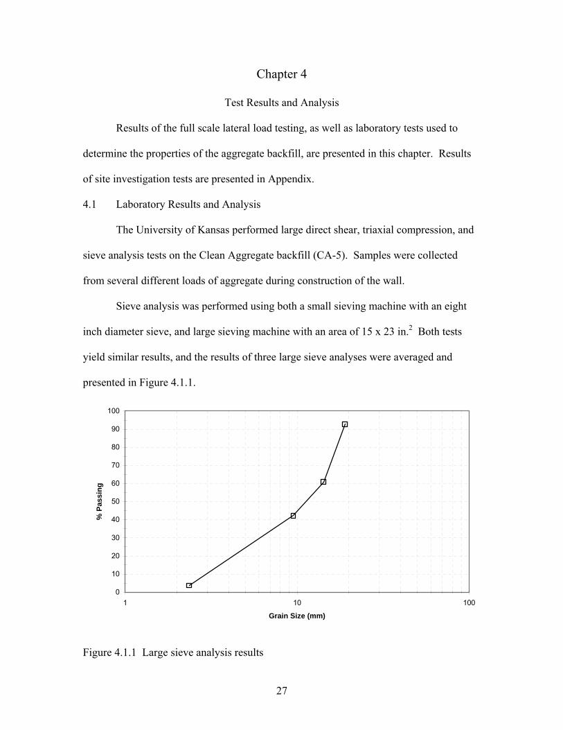
Sieve analysis was performed using both a small sieving machine with an eight
inch diameter sieve, and large sieving machine with an area of 15 x 23 in.2 Both tests
yield similar results, and the results of three large sieve analyses were averaged and
presented in Figure 4.1.1.
0
10
20
30
40
50
60
70
80
90
100
1 10 100
Grain Size (mm)
% P
assi
ng
Figure 4.1.1 Large sieve analysis results
28
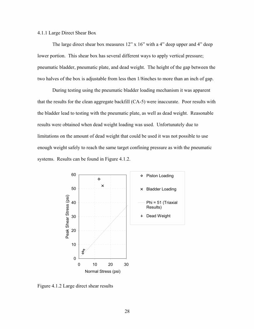
4.1.1 Large Direct Shear Box
The large direct shear box measures 12” x 16” with a 4” deep upper and 4” deep
lower portion. This shear box has several different ways to apply vertical pressure;
pneumatic bladder, pneumatic plate, and dead weight. The height of the gap between the
two halves of the box is adjustable from less then 1/8inches to more than an inch of gap.
During testing using the pneumatic bladder loading mechanism it was apparent
that the results for the clean aggregate backfill (CA-5) were inaccurate. Poor results with
the bladder lead to testing with the pneumatic plate, as well as dead weight. Reasonable
results were obtained when dead weight loading was used. Unfortunately due to
limitations on the amount of dead weight that could be used it was not possible to use
enough weight safely to reach the same target confining pressure as with the pneumatic
systems. Results can be found in Figure 4.1.2.
0
10
20
30
40
50
60
0 10 20 30
Normal Stress (psi)
Peak
She
ar S
tress
(psi
)
Piston Loading
Bladder Loading
Phi = 51 (TriaxialResults)
Dead Weight
Figure 4.1.2 Large direct shear results
29
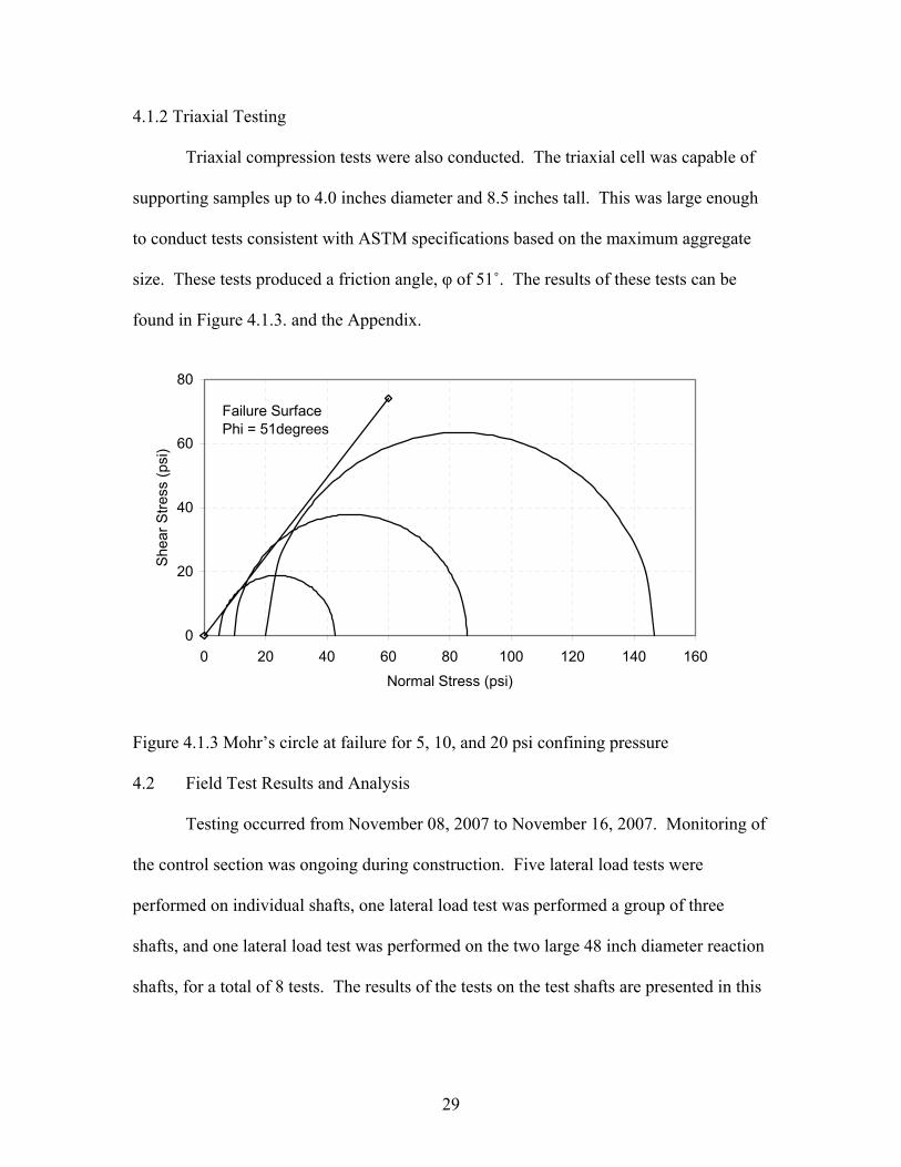
4.1.2 Triaxial Testing
Triaxial compression tests were also conducted. The triaxial cell was capable of
supporting samples up to 4.0 inches diameter and 8.5 inches tall. This was large enough
to conduct tests consistent with ASTM specifications based on the maximum aggregate
size. These tests produced a friction angle, φ of 51˚. The results of these tests can be
found in Figure 4.1.3. and the Appendix.
0
20
40
60
80
0 20 40 60 80 100 120 140 160
Normal Stress (psi)
Shea
r Stre
ss (p
si)
Failure SurfacePhi = 51degrees
Figure 4.1.3 Mohr’s circle at failure for 5, 10, and 20 psi confining pressure
4.2 Field Test Results and Analysis
Testing occurred from November 08, 2007 to November 16, 2007. Monitoring of
the control section was ongoing during construction. Five lateral load tests were
performed on individual shafts, one lateral load test was performed a group of three
shafts, and one lateral load test was performed on the two large 48 inch diameter reaction
shafts, for a total of 8 tests. The results of the tests on the test shafts are presented in this
30
document. Loads and deflections associated with a shaft were measured at one foot
above the ground surface
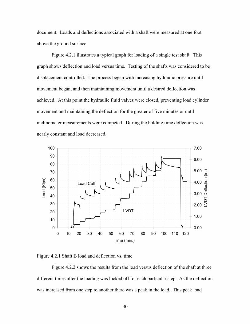
Figure 4.2.1 illustrates a typical graph for loading of a single test shaft. This
graph shows deflection and load versus time. Testing of the shafts was considered to be
displacement controlled. The process began with increasing hydraulic pressure until
movement began, and then maintaining movement until a desired deflection was
achieved. At this point the hydraulic fluid valves were closed, preventing load cylinder
movement and maintaining the deflection for the greater of five minutes or until
inclinometer measurements were competed. During the holding time deflection was
nearly constant and load decreased.
0
10
20
30
40
50
60
70
80
90
100
0 10 20 30 40 50 60 70 80 90 100 110 120
Time (min.)
Load
(Kip
s)
0.00
1.00
2.00
3.00
4.00
5.00
6.00
7.00
LVD
T D
efle
ctio
n (in
.)
Load Cell
LVDT
Figure 4.2.1 Shaft B load and deflection vs. time
Figure 4.2.2 shows the results from the load versus deflection of the shaft at three
different times after the loading was locked off for each particular step. As the deflection
was increased from one step to another there was a peak in the load. This peak load
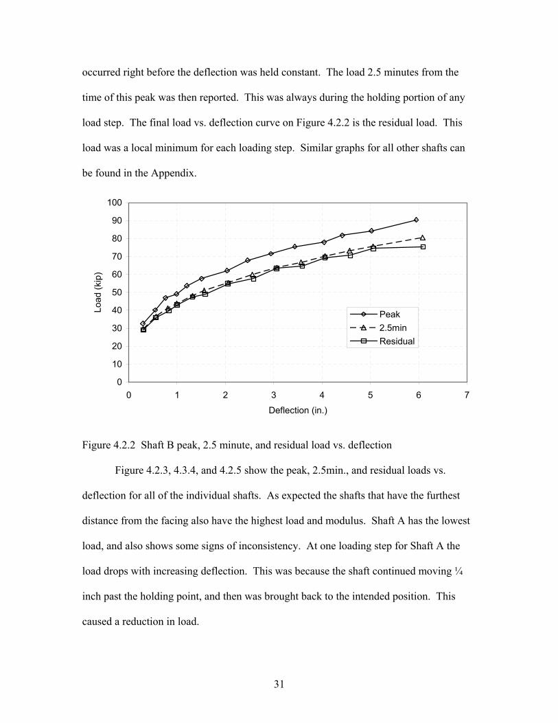
31
occurred right before the deflection was held constant. The load 2.5 minutes from the
time of this peak was then reported. This was always during the holding portion of any
load step. The final load vs. deflection curve on Figure 4.2.2 is the residual load. This
load was a local minimum for each loading step. Similar graphs for all other shafts can
be found in the Appendix.
0
10
20
30
40
50
60
70
80
90
100
0 1 2 3 4 5 6 7
Deflection (in.)
Load
(kip
)
Peak2.5minResidual
Figure 4.2.2 Shaft B peak, 2.5 minute, and residual load vs. deflection
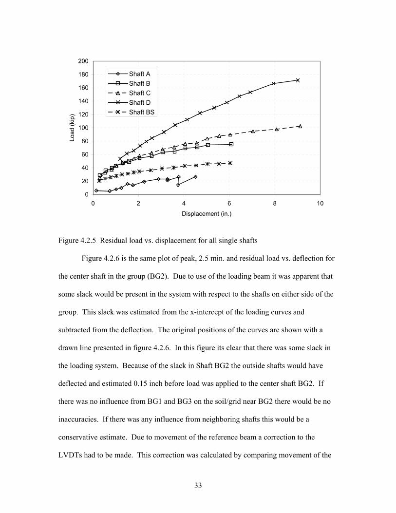
Figure 4.2.3, 4.3.4, and 4.2.5 show the peak, 2.5min., and residual loads vs.
deflection for all of the individual shafts. As expected the shafts that have the furthest
distance from the facing also have the highest load and modulus. Shaft A has the lowest
load, and also shows some signs of inconsistency. At one loading step for Shaft A the
load drops with increasing deflection. This was because the shaft continued moving ¼
inch past the holding point, and then was brought back to the intended position. This
caused a reduction in load.

32
0
20
40
60
80
100
120
140
160
180
200
0 2 4 6 8 10
Displacement (in.)
Load
(kip
)Shaft AShaft BShaft CShaft DShaft BS
Figure 4.2.3 Peak load vs. deflection for all single shafts
0
20
40
60
80
100
120
140
160
180
200
0 2 4 6 8 10
Displacement (in.)
Load
(kip
)
Shaft AShaft BShaft CShaft DShaft BS
Figure 4.2.4 Load at 2.5 minutes vs. deflection for all single shafts
33
0
20
40
60
80
100
120
140
160
180
200
0 2 4 6 8 10
Displacement (in.)
Load
(kip
)Shaft AShaft BShaft CShaft DShaft BS
Figure 4.2.5 Residual load vs. displacement for all single shafts
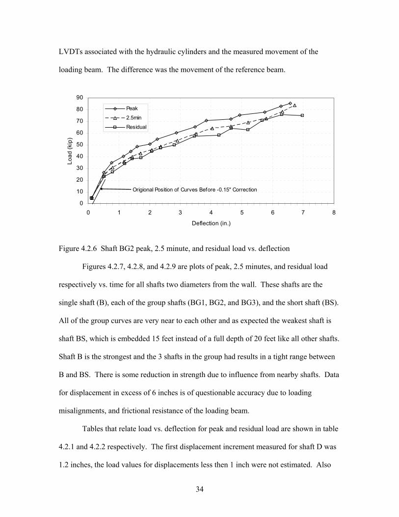
Figure 4.2.6 is the same plot of peak, 2.5 min. and residual load vs. deflection for
the center shaft in the group (BG2). Due to use of the loading beam it was apparent that
some slack would be present in the system with respect to the shafts on either side of the
group. This slack was estimated from the x-intercept of the loading curves and
subtracted from the deflection. The original positions of the curves are shown with a
drawn line presented in figure 4.2.6. In this figure its clear that there was some slack in
the loading system. Because of the slack in Shaft BG2 the outside shafts would have
deflected and estimated 0.15 inch before load was applied to the center shaft BG2. If
there was no influence from BG1 and BG3 on the soil/grid near BG2 there would be no
inaccuracies. If there was any influence from neighboring shafts this would be a
conservative estimate. Due to movement of the reference beam a correction to the
LVDTs had to be made. This correction was calculated by comparing movement of the
34
LVDTs associated with the hydraulic cylinders and the measured movement of the
loading beam. The difference was the movement of the reference beam.
0
10
20
30
40
50
60
70
80
90
0 1 2 3 4 5 6 7 8
Deflection (in.)
Load
(kip
)
Peak
2.5min
Residual
Origional Position of Curves Before -0.15" Correction
Figure 4.2.6 Shaft BG2 peak, 2.5 minute, and residual load vs. deflection
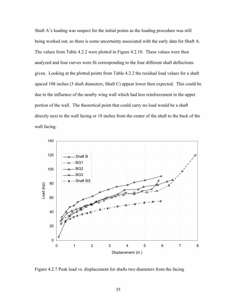
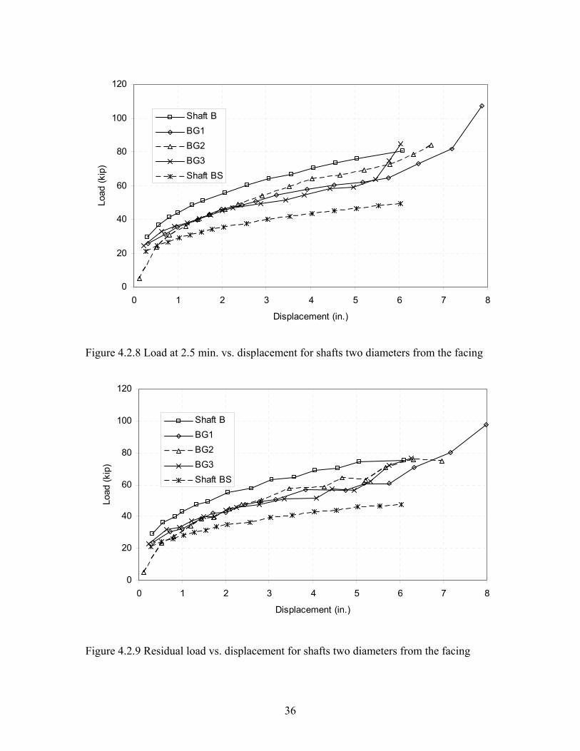
Figures 4.2.7, 4.2.8, and 4.2.9 are plots of peak, 2.5 minutes, and residual load
respectively vs. time for all shafts two diameters from the wall. These shafts are the
single shaft (B), each of the group shafts (BG1, BG2, and BG3), and the short shaft (BS).
All of the group curves are very near to each other and as expected the weakest shaft is
shaft BS, which is embedded 15 feet instead of a full depth of 20 feet like all other shafts.
Shaft B is the strongest and the 3 shafts in the group had results in a tight range between
B and BS. There is some reduction in strength due to influence from nearby shafts. Data
for displacement in excess of 6 inches is of questionable accuracy due to loading
misalignments, and frictional resistance of the loading beam.
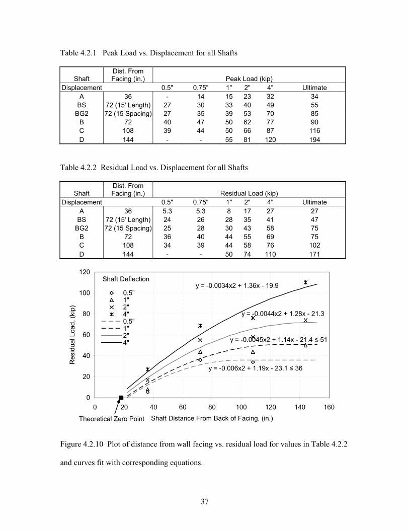
Tables that relate load vs. deflection for peak and residual load are shown in table
4.2.1 and 4.2.2 respectively. The first displacement increment measured for shaft D was
1.2 inches, the load values for displacements less then 1 inch were not estimated. Also
35
Shaft A’s loading was suspect for the initial points as the loading procedure was still
being worked out, so there is some uncertainty associated with the early data for Shaft A.
The values from Table 4.2.2 were plotted in Figure 4.2.10. These values were then
analyzed and four curves were fit corresponding to the four different shaft deflections
given. Looking at the plotted points from Table 4.2.2 the residual load values for a shaft
spaced 108 inches (3 shaft diameters, Shaft C) appear lower then expected. This could be
due to the influence of the nearby wing wall which had less reinforcement in the upper
portion of the wall. The theoretical point that could carry no load would be a shaft
directly next to the wall facing or 18 inches from the center of the shaft to the back of the
wall facing.
0
20
40
60
80
100
120
140
0 1 2 3 4 5 6 7 8
Displacement (in.)
Load
(kip
)
Shaft BBG1BG2BG3Shaft BS
Figure 4.2.7 Peak load vs. displacement for shafts two diameters from the facing
36
0
20
40
60
80
100
120
0 1 2 3 4 5 6 7 8
Displacement (in.)
Load
(kip
)Shaft BBG1BG2BG3Shaft BS
Figure 4.2.8 Load at 2.5 min. vs. displacement for shafts two diameters from the facing
0
20
40
60
80
100
120
0 1 2 3 4 5 6 7 8
Displacement (in.)
Load
(kip
)
Shaft BBG1BG2BG3Shaft BS
Figure 4.2.9 Residual load vs. displacement for shafts two diameters from the facing
37
Table 4.2.1 Peak Load vs. Displacement for all Shafts
Shaft Dist. From Facing (in.) Peak Load (kip)
Displacement 0.5" 0.75" 1" 2" 4" Ultimate A 36 - 14 15 23 32 34
BS 72 (15' Length) 27 30 33 40 49 55 BG2 72 (15 Spacing) 27 35 39 53 70 85
B 72 40 47 50 62 77 90 C 108 39 44 50 66 87 116 D 144 - - 55 81 120 194
Table 4.2.2 Residual Load vs. Displacement for all Shafts
Shaft Dist. From Facing (in.) Residual Load (kip)
Displacement 0.5" 0.75" 1" 2" 4" Ultimate A 36 5.3 5.3 8 17 27 27
BS 72 (15' Length) 24 26 28 35 41 47 BG2 72 (15 Spacing) 25 28 30 43 58 75
B 72 36 40 44 55 69 75 C 108 34 39 44 58 76 102 D 144 - - 50 74 110 171
0
20
40
60
80
100
120
0 20 40 60 80 100 120 140 160
Shaft Distance From Back of Facing, (in.)
Res
idua
l Loa
d, (k
ip)
0.5"1"2"4"0.5" 1"2"4"
Shaft Deflection
Theoretical Zero Point
y = -0.0034x2 + 1.36x - 19.9
y = -0.0044x2 + 1.28x - 21.3
y = -0.0045x2 + 1.14x - 21.4 ≤ 51
y = -0.006x2 + 1.19x - 23.1 ≤ 36
Figure 4.2.10 Plot of distance from wall facing vs. residual load for values in Table 4.2.2
and curves fit with corresponding equations.
38
4.3 Wall Deflections
Wall deflections were measured using photogametry as described in chapter 3.
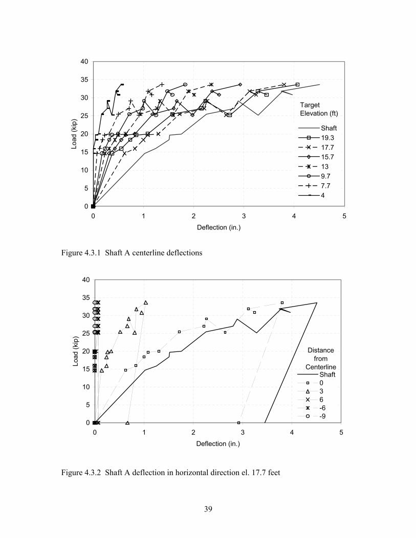
The results will be reported and analyzed in the next pages. Figure 4.3.1 shows the peak
load vs. deflections of the wall facing for the targets that are mounted on the centerline of
Shaft A, as well as the shaft itself. Due to the loading problem with Shaft A discussed
earlier, this particular plot contains more fluctuations than other plots. As expected the
shaft moved more than the top of the wall and the top of the wall moved more than the
bottom. Figure 4.3.2 shows the deflection of targets for Shaft A along the horizontal axis
at an elevation of 17.7 feet, as well as the shaft deflection. As expected the shaft moves
more then the target at the centerline of the shaft, and wall movement decreased with
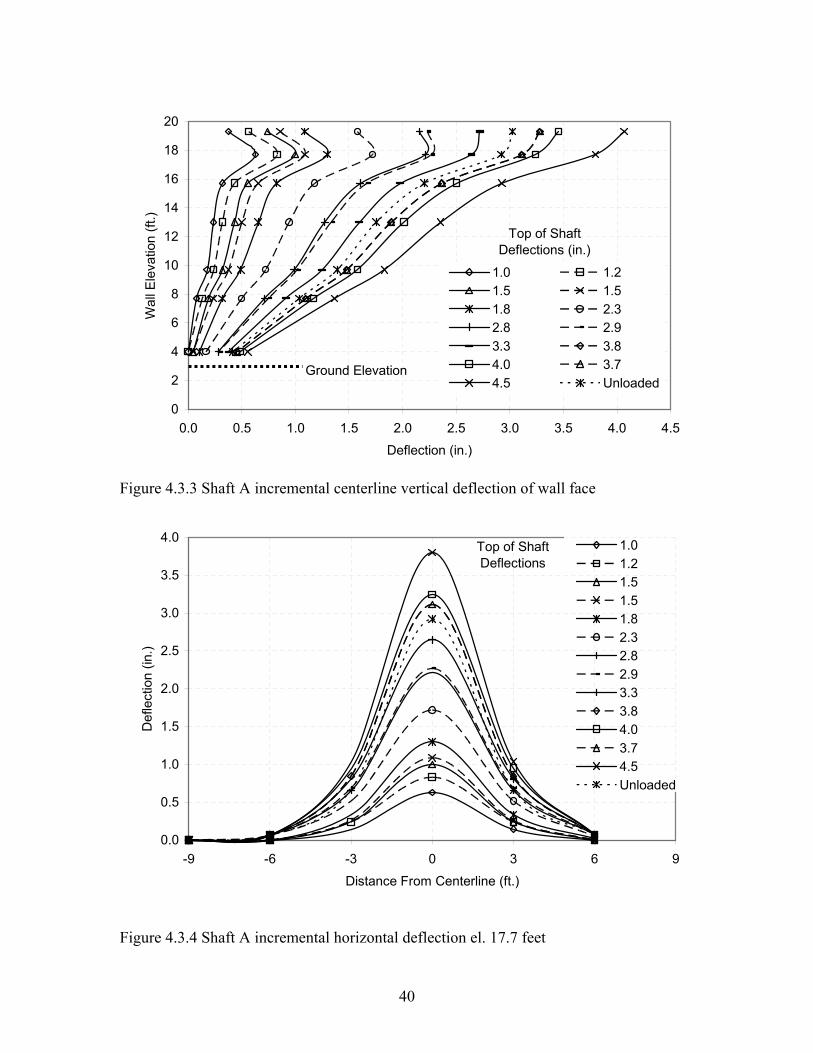
distance from the centerline. Figure 4.3.3 shows the deflection of the facing at the shaft
centerline for each load step. The Y-axis shows elevation of the target, and the X-axis
shows the deflection of the targets. From this figure an interesting bulge at 17.7feet was
found showing that there was increased movement at an elevation below the top. This
indicates that the wall is not just tipping over, but is actually moving horizontally
depending on the lateral pressure placed on it. Figure 4.3.4 shows the deflection of the
facing in the horizontal direction at an elevation of 17.7 feet for each displacement
increment. The behavior was as expected with much more movement near the centerline
of the shaft and less movement as the horizontal distance increased. This figure shows
that significant deflections of the wall were limited to within six feet of the centerline of
loading for Shaft A. The influence distance in the horizontal direction was determined
from Figure 4.3.4.
39
0
5
10
15
20
25
30
35
40
0 1 2 3 4 5
Deflection (in.)
Load
(kip
)
Shaft19.317.715.7139.77.74
Target Elevation (ft)
Figure 4.3.1 Shaft A centerline deflections
0
5
10
15
20
25
30
35
40
0 1 2 3 4 5
Deflection (in.)
Load
(kip
)
Shaft036-6-9
Distance from
Centerline
Figure 4.3.2 Shaft A deflection in horizontal direction el. 17.7 feet
40
0
2
4
6
8
10
12
14
16
18
20
0.0 0.5 1.0 1.5 2.0 2.5 3.0 3.5 4.0 4.5
Deflection (in.)
Wal
l Ele
vatio
n (ft
.)
1.0 1.21.5 1.51.8 2.32.8 2.93.3 3.84.0 3.74.5 Unloaded
Top of Shaft Deflections (in.)
Ground Elevation
Figure 4.3.3 Shaft A incremental centerline vertical deflection of wall face
0.0
0.5
1.0
1.5
2.0
2.5
3.0
3.5
4.0
-9 -6 -3 0 3 6 9
Distance From Centerline (ft.)
Def
lect
ion
(in.)
1.01.21.51.51.82.32.82.93.33.84.03.74.5Unloaded
Top of Shaft Deflections
Figure 4.3.4 Shaft A incremental horizontal deflection el. 17.7 feet
41
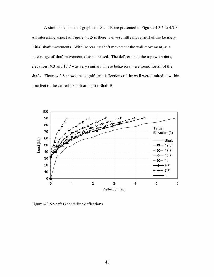
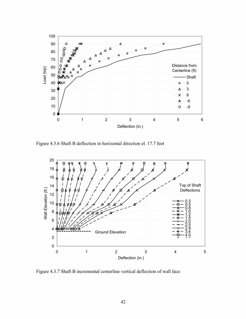
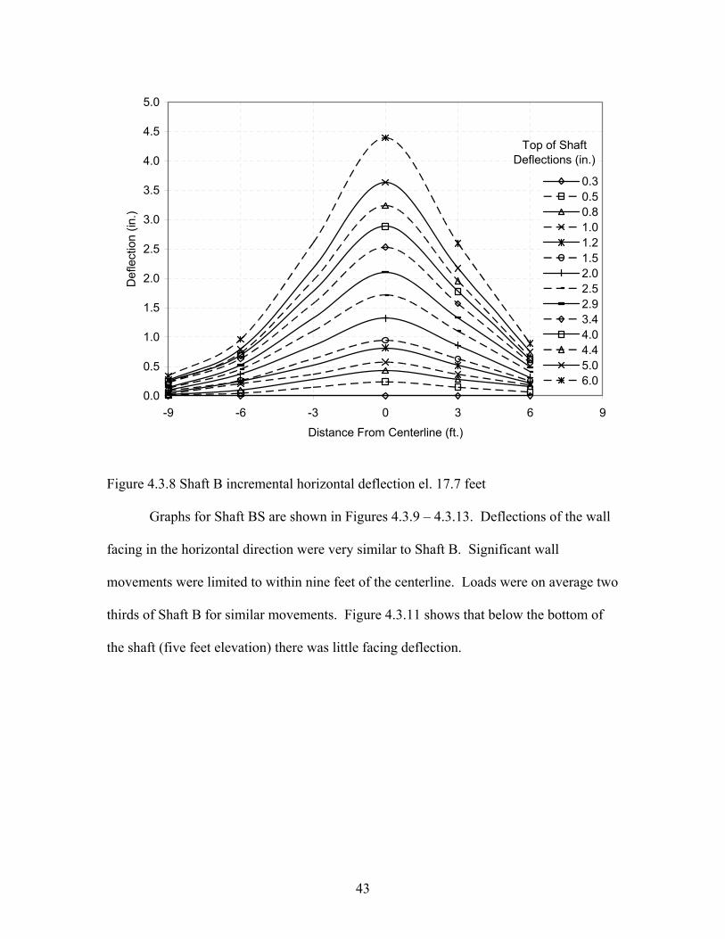
A similar sequence of graphs for Shaft B are presented in Figures 4.3.5 to 4.3.8.
An interesting aspect of Figure 4.3.5 is there was very little movement of the facing at
initial shaft movements. With increasing shaft movement the wall movement, as a
percentage of shaft movement, also increased. The deflection at the top two points,
elevation 19.3 and 17.7 was very similar. These behaviors were found for all of the
shafts. Figure 4.3.8 shows that significant deflections of the wall were limited to within
nine feet of the centerline of loading for Shaft B.
0
10
20
30
40
50
60
70
80
90
100
0 1 2 3 4 5 6
Deflection (in.)
Load
(kip
)
Shaft19.317.715.7139.77.74
Target Elevation (ft)
Figure 4.3.5 Shaft B centerline deflections
42
0
10
20
30
40
50
60
70
80
90
100
0 1 2 3 4 5 6
Deflection (in.)
Load
(kip
)
Shaft036-6-9
Distance from Centerline (ft)
Figure 4.3.6 Shaft B deflection in horizontal direction el. 17.7 feet
0
2
4
6
8
10
12
14
16
18
20
0 1 2 3 4 5Deflection (in.)
Wal
l Ele
vatio
n (ft
.)
0.30.50.81.01.21.52.02.52.93.44.04 4
Top of Shaft Deflections
Ground Elevation
Figure 4.3.7 Shaft B incremental centerline vertical deflection of wall face
43
0.0
0.5
1.0
1.5
2.0
2.5
3.0
3.5
4.0
4.5
5.0
-9 -6 -3 0 3 6 9
Distance From Centerline (ft.)
Def
lect
ion
(in.)
0.30.50.81.01.21.52.02.52.93.44.04.45.06.0
Top of Shaft Deflections (in.)
Figure 4.3.8 Shaft B incremental horizontal deflection el. 17.7 feet
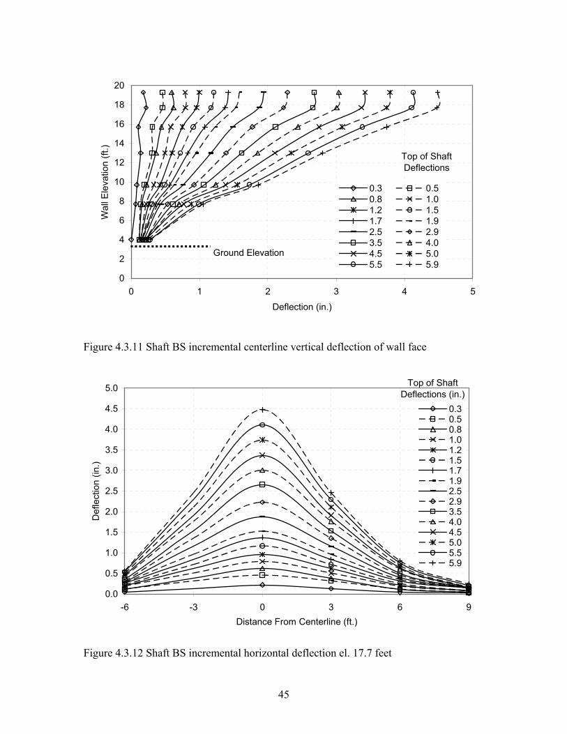
Graphs for Shaft BS are shown in Figures 4.3.9 – 4.3.13. Deflections of the wall
facing in the horizontal direction were very similar to Shaft B. Significant wall
movements were limited to within nine feet of the centerline. Loads were on average two
thirds of Shaft B for similar movements. Figure 4.3.11 shows that below the bottom of
the shaft (five feet elevation) there was little facing deflection.

44
0
10
20
30
40
50
60
0 1 2 3 4 5 6
Deflection (in.)
Load
(kip
)
Shaft19.317.715.7139.77.74
Target Elevation (ft)
Figure 4.3.9 Shaft BS centerline deflections
0
10
20
30
40
50
60
0 1 2 3 4 5 6
Deflection (in.)
Load
(kip
)
Shaft03669
Distance from Centerline (ft)
Figure 4.3.10 Shaft BS deflection in horizontal direction el. 17.7 feet
45
0
2
4
6
8
10
12
14
16
18
20
0 1 2 3 4 5
Deflection (in.)
Wal
l Ele
vatio
n (ft
.)
0.3 0.50.8 1.01.2 1.51.7 1.92.5 2.93.5 4.04.5 5.05.5 5.9
Top of Shaft Deflections
Ground Elevation
Figure 4.3.11 Shaft BS incremental centerline vertical deflection of wall face
0.0
0.5
1.0
1.5
2.0
2.5
3.0
3.5
4.0
4.5
5.0
-6 -3 0 3 6 9Distance From Centerline (ft.)
Def
lect
ion
(in.)
0.30.50.81.01.21.51.71.92.52.93.54.04.55.05.55.9
Top of Shaft Deflections (in.)
Figure 4.3.12 Shaft BS incremental horizontal deflection el. 17.7 feet
46
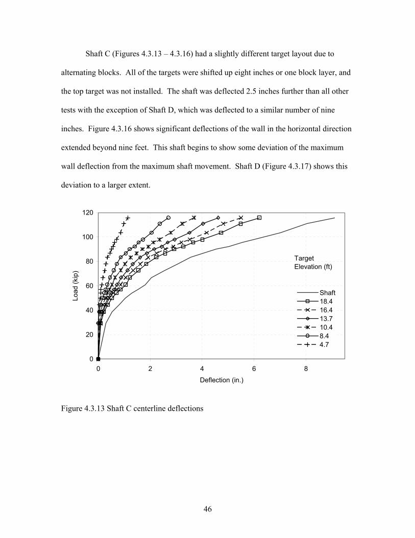
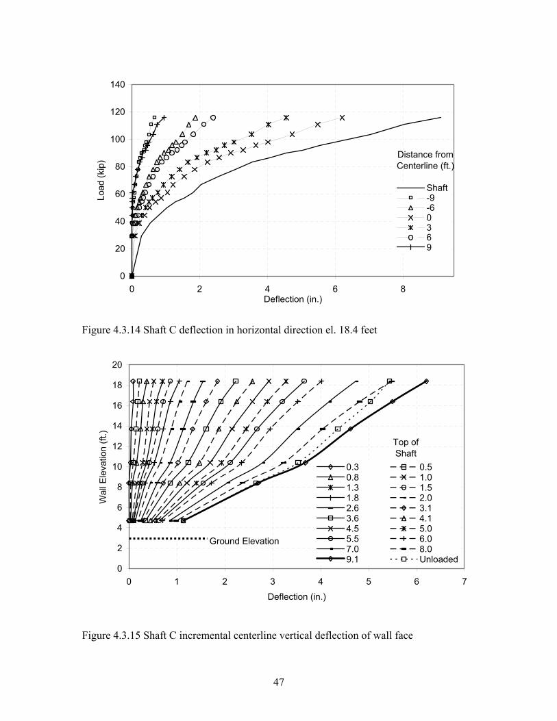
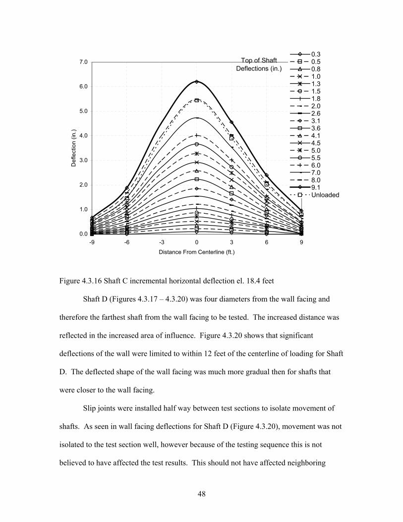
Shaft C (Figures 4.3.13 – 4.3.16) had a slightly different target layout due to
alternating blocks. All of the targets were shifted up eight inches or one block layer, and
the top target was not installed. The shaft was deflected 2.5 inches further than all other
tests with the exception of Shaft D, which was deflected to a similar number of nine
inches. Figure 4.3.16 shows significant deflections of the wall in the horizontal direction
extended beyond nine feet. This shaft begins to show some deviation of the maximum
wall deflection from the maximum shaft movement. Shaft D (Figure 4.3.17) shows this
deviation to a larger extent.
0
20
40
60
80
100
120
0 2 4 6 8
Deflection (in.)
Load
(kip
)
Shaft18.416.413.710.48.44.7
Target Elevation (ft)
Figure 4.3.13 Shaft C centerline deflections
47
0
20
40
60
80
100
120
140
0 2 4 6 8Deflection (in.)
Load
(kip
)
Shaft-9-60369
Distance from Centerline (ft.)
Figure 4.3.14 Shaft C deflection in horizontal direction el. 18.4 feet
0
2
4
6
8
10
12
14
16
18
20
0 1 2 3 4 5 6 7
Deflection (in.)
Wal
l Ele
vatio
n (ft
.)
0.3 0.50.8 1.01.3 1.51.8 2.02.6 3.13.6 4.14.5 5.05.5 6.07.0 8.09.1 Unloaded
Top of Shaft
Ground Elevation
Figure 4.3.15 Shaft C incremental centerline vertical deflection of wall face
48
0.0
1.0
2.0
3.0
4.0
5.0
6.0
7.0
-9 -6 -3 0 3 6 9
Distance From Centerline (ft.)
Def
lect
ion
(in.)
0.30.50.81.01.31.51.82.02.63.13.64.14.55.05.56.07.08.09.1Unloaded
Top of Shaft Deflections (in.)
Figure 4.3.16 Shaft C incremental horizontal deflection el. 18.4 feet
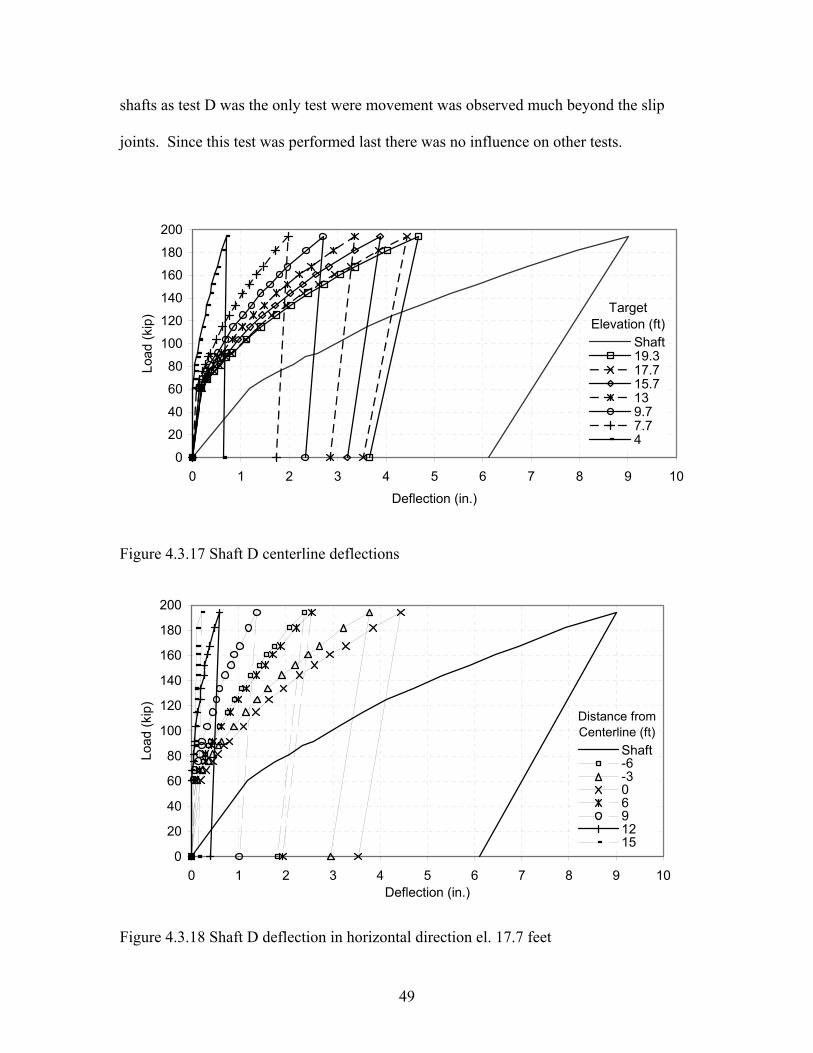
Shaft D (Figures 4.3.17 – 4.3.20) was four diameters from the wall facing and
therefore the farthest shaft from the wall facing to be tested. The increased distance was
reflected in the increased area of influence. Figure 4.3.20 shows that significant
deflections of the wall were limited to within 12 feet of the centerline of loading for Shaft
D. The deflected shape of the wall facing was much more gradual then for shafts that
were closer to the wall facing.
Slip joints were installed half way between test sections to isolate movement of
shafts. As seen in wall facing deflections for Shaft D (Figure 4.3.20), movement was not
isolated to the test section well, however because of the testing sequence this is not
believed to have affected the test results. This should not have affected neighboring
49
shafts as test D was the only test were movement was observed much beyond the slip
joints. Since this test was performed last there was no influence on other tests.
0
20
40
60
80
100
120
140
160
180
200
0 1 2 3 4 5 6 7 8 9 10
Deflection (in.)
Load
(kip
)
Shaft19.317.715.7139.77.74
Target Elevation (ft)
Figure 4.3.17 Shaft D centerline deflections
0
20
40
60
80
100
120
140
160
180
200
0 1 2 3 4 5 6 7 8 9 10Deflection (in.)
Load
(kip
)
Shaft-6-30691215
Distance from Centerline (ft)
Figure 4.3.18 Shaft D deflection in horizontal direction el. 17.7 feet

50
0
2
4
6
8
10
12
14
16
18
20
0.0 0.5 1.0 1.5 2.0 2.5 3.0 3.5 4.0 4.5 5.0
Deflection (in.)
Wal
l Ele
vatio
n (ft
.)
1.2 1.51.8 2.12.3 2.63.1 3.64.1 4.75.3 5.96.4 6.97.9 9.0Unloaded
Top of Shaft Deflections
Ground Elevation
Figure 4.3.19 Shaft D incremental centerline vertical deflection of wall face
0.0
0.5
1.0
1.5
2.0
2.5
3.0
3.5
4.0
4.5
5.0
-6 -3 0 3 6 9 12 15
Distance From Centerline (ft.)
Def
lect
ion
(in.)
1.21.51.82.12.32.63.13.64.14.75.35.96.46.97.99.0Unloaded
Top of Shaft Deflections (in.)
Figure 4.3.20 Shaft D incremental horizontal deflection el. 17.7 feet
51
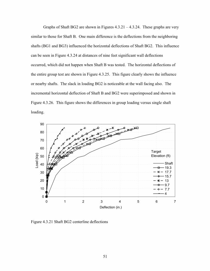
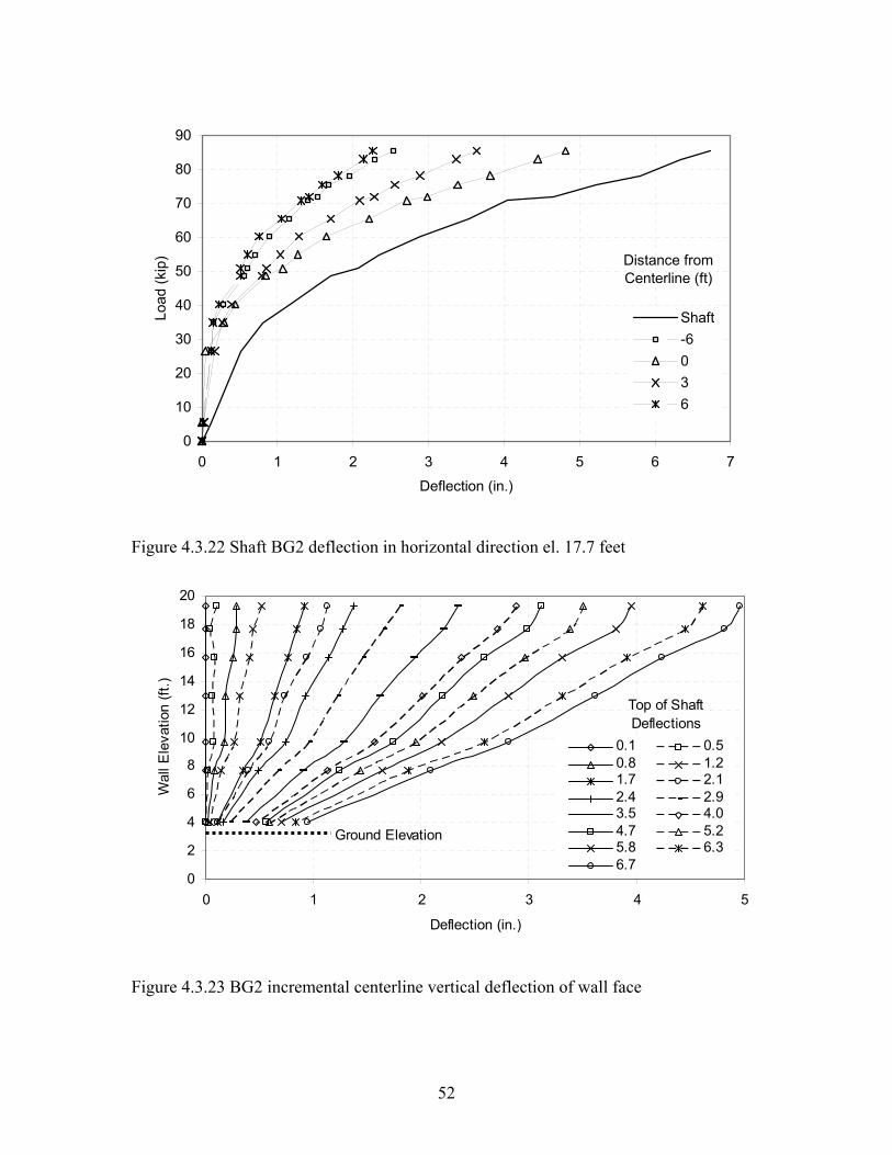
Graphs of Shaft BG2 are shown in Figures 4.3.21 – 4.3.24. These graphs are very
similar to those for Shaft B. One main difference is the deflections from the neighboring
shafts (BG1 and BG3) influenced the horizontal deflections of Shaft BG2. This influence
can be seen in Figure 4.3.24 at distances of nine feet significant wall deflections
occurred, which did not happen when Shaft B was tested. The horizontal deflections of
the entire group test are shown in Figure 4.3.25. This figure clearly shows the influence
or nearby shafts. The slack in loading BG2 is noticeable at the wall facing also. The
incremental horizontal deflection of Shaft B and BG2 were superimposed and shown in
Figure 4.3.26. This figure shows the differences in group loading versus single shaft
loading.
0
10
20
30
40
50
60
70
80
90
0 1 2 3 4 5 6 7
Deflection (in.)
Load
(kip
)
Shaft19.317.715.7139.77.74
Target Elevation (ft)
Figure 4.3.21 Shaft BG2 centerline deflections
52
0
10
20
30
40
50
60
70
80
90
0 1 2 3 4 5 6 7
Deflection (in.)
Load
(kip
)
Shaft-6036
Distance from Centerline (ft)
Figure 4.3.22 Shaft BG2 deflection in horizontal direction el. 17.7 feet
0
2
4
6
8
10
12
14
16
18
20
0 1 2 3 4 5
Deflection (in.)
Wal
l Ele
vatio
n (ft
.)
0.1 0.50.8 1.21.7 2.12.4 2.93.5 4.04.7 5.25.8 6.36.7
Top of Shaft Deflections
Ground Elevation
Figure 4.3.23 BG2 incremental centerline vertical deflection of wall face

53
0
1
2
3
4
5
6
-9 -6 -3 0 3 6 9
Distance From Centerline (ft.)
Def
lect
ion
(in.)
0.10.50.81.21.72.12.42.93.54.04.75.25.86.36.7
Top of Shaft Deflections (in.)
Figure 4.3.24 Shaft BG2 incremental horizontal deflection el. 17.7 feet (portion of Figure
4.3.25)
0
1
2
3
4
5
6
-21 -18 -15 -12 -9 -6 -3 0 3 6 9 12 15 18 21 24
Distance From Centerline (ft.)
Def
lect
ion
(in.)
0.10.50.81.21.72.12.42.93.54.04.75.25.86.36.7
Top of Shaft BG2 Deflections (in.)
Figure 4.3.25 Shafts BG incremental horizontal deflection el. 17.7 feet
54
0.0
0.5
1.0
1.5
2.0
2.5
3.0
3.5
4.0
4.5
5.0
-9 -6 -3 0 3 6 9
Distance From Centerline (ft.)
Def
lect
ion
(in.)
0.5 1.02.0 4.05.0 6.00.5 1.02.0 4.05.0 6.0
Top of Shaft Deflections (in.)Shaft B
Shaft BG2
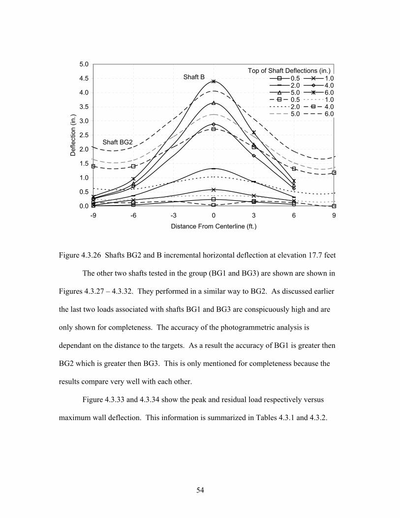
Figure 4.3.26 Shafts BG2 and B incremental horizontal deflection at elevation 17.7 feet
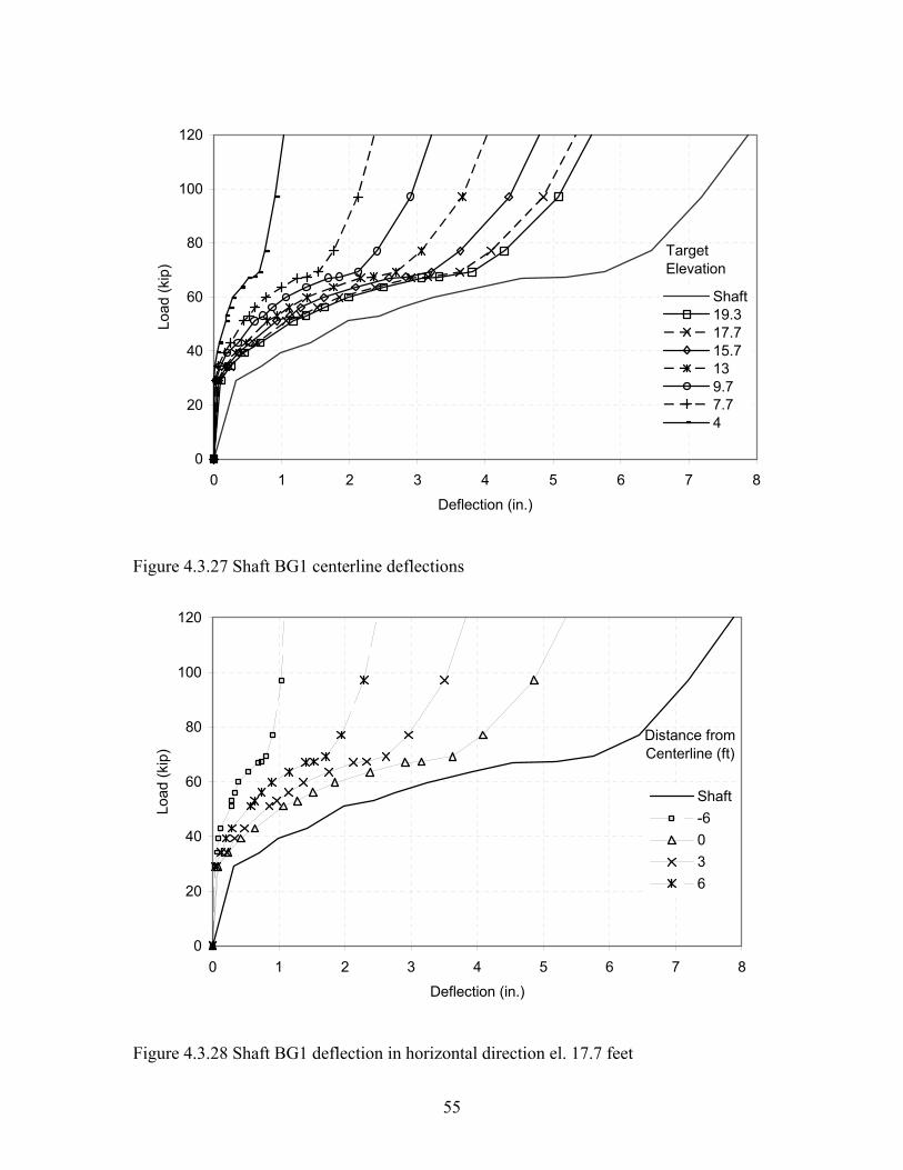
The other two shafts tested in the group (BG1 and BG3) are shown are shown in
Figures 4.3.27 – 4.3.32. They performed in a similar way to BG2. As discussed earlier
the last two loads associated with shafts BG1 and BG3 are conspicuously high and are
only shown for completeness. The accuracy of the photogrammetric analysis is
dependant on the distance to the targets. As a result the accuracy of BG1 is greater then
BG2 which is greater then BG3. This is only mentioned for completeness because the
results compare very well with each other.
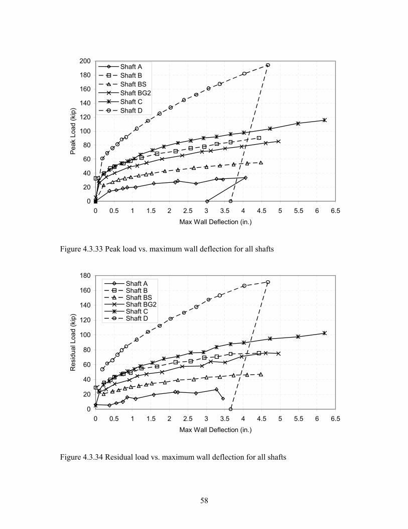
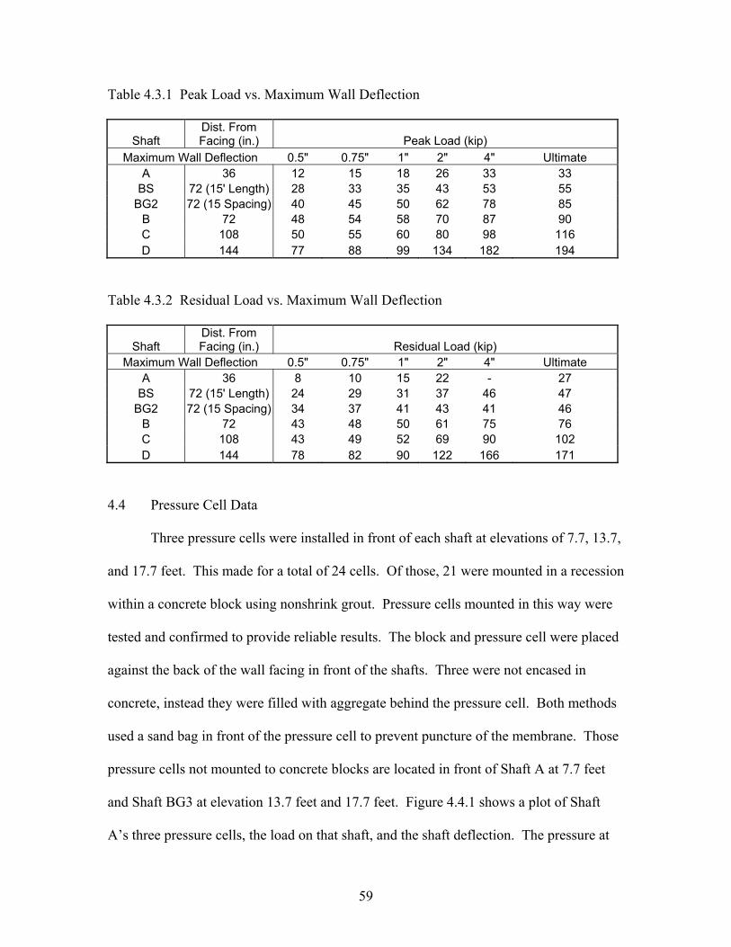
Figure 4.3.33 and 4.3.34 show the peak and residual load respectively versus
maximum wall deflection. This information is summarized in Tables 4.3.1 and 4.3.2.
55
0
20
40
60
80
100
120
0 1 2 3 4 5 6 7 8
Deflection (in.)
Load
(kip
)
Shaft19.317.715.7139.77.74
Target Elevation (f )
Figure 4.3.27 Shaft BG1 centerline deflections
0
20
40
60
80
100
120
0 1 2 3 4 5 6 7 8
Deflection (in.)
Load
(kip
)
Shaft-6036
Distance from Centerline (ft)
Figure 4.3.28 Shaft BG1 deflection in horizontal direction el. 17.7 feet
56
0
2
4
6
8
10
12
14
16
18
20
0 1 2 3 4 5 6
Deflection (in.)
Wal
l Ele
vatio
n (ft
.) 0.30.71.01.42.02.42.83.23.94.55.25.86.47.27.9
Top of Shaft
Ground Elevation
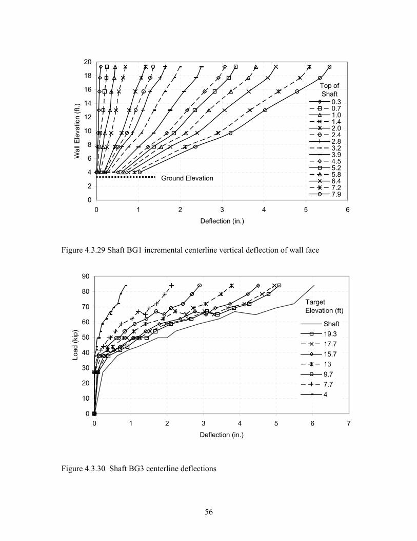
Figure 4.3.29 Shaft BG1 incremental centerline vertical deflection of wall face
0
10
20
30
40
50
60
70
80
90
0 1 2 3 4 5 6 7
Deflection (in.)
Load
(kip
)
Shaft19.317.715.7139.77.74
Target Elevation (ft)
Figure 4.3.30 Shaft BG3 centerline deflections
57
0
10
20
30
40
50
60
70
80
90
0 1 2 3 4 5 6 7
Deflection (in.)
Load
(kip
) Shaft-6-30369
Distance from Centerline (ft)
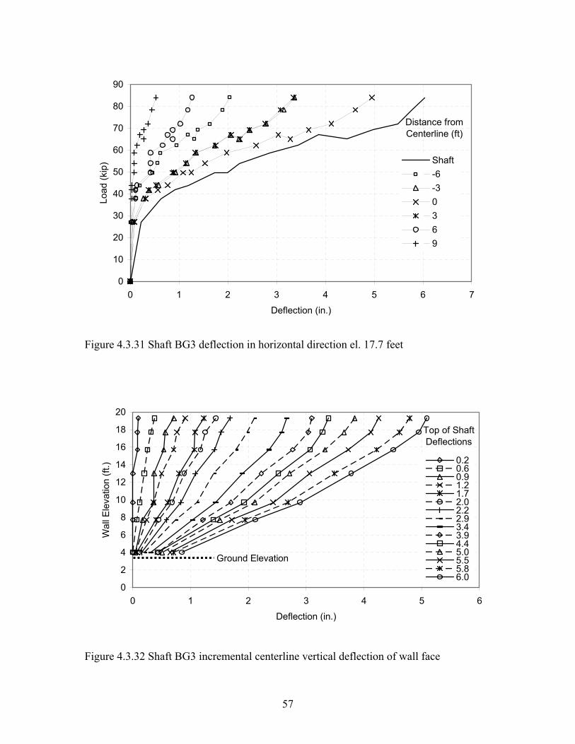
Figure 4.3.31 Shaft BG3 deflection in horizontal direction el. 17.7 feet
0
2
4
6
8
10
12
14
16
18
20
0 1 2 3 4 5 6
Deflection (in.)
Wal
l Ele
vatio
n (ft
.) 0.20.60.91.21.72.02.22.93.43.94.45.05.55.86.0
Top of Shaft Deflections
Ground Elevation
Figure 4.3.32 Shaft BG3 incremental centerline vertical deflection of wall face
58
0
20
40
60
80
100
120
140
160
180
200
0 0.5 1 1.5 2 2.5 3 3.5 4 4.5 5 5.5 6 6.5
Max Wall Deflection (in.)
Peak
Loa
d (k
ip)
Shaft AShaft BShaft BSShaft BG2Shaft CShaft D
Figure 4.3.33 Peak load vs. maximum wall deflection for all shafts
0
20
40
60
80
100
120
140
160
180
0 0.5 1 1.5 2 2.5 3 3.5 4 4.5 5 5.5 6 6.5
Max Wall Deflection (in.)
Res
idua
l Loa
d (k
ip)
Shaft AShaft BShaft BSShaft BG2Shaft CShaft D
Figure 4.3.34 Residual load vs. maximum wall deflection for all shafts
59
Table 4.3.1 Peak Load vs. Maximum Wall Deflection
Shaft Dist. From Facing (in.) Peak Load (kip)
Maximum Wall Deflection 0.5" 0.75" 1" 2" 4" Ultimate A 36 12 15 18 26 33 33
BS 72 (15' Length) 28 33 35 43 53 55 BG2 72 (15 Spacing) 40 45 50 62 78 85
B 72 48 54 58 70 87 90 C 108 50 55 60 80 98 116 D 144 77 88 99 134 182 194
Table 4.3.2 Residual Load vs. Maximum Wall Deflection
Shaft Dist. From Facing (in.) Residual Load (kip)
Maximum Wall Deflection 0.5" 0.75" 1" 2" 4" Ultimate A 36 8 10 15 22 - 27
BS 72 (15' Length) 24 29 31 37 46 47 BG2 72 (15 Spacing) 34 37 41 43 41 46
B 72 43 48 50 61 75 76 C 108 43 49 52 69 90 102 D 144 78 82 90 122 166 171
4.4 Pressure Cell Data
Three pressure cells were installed in front of each shaft at elevations of 7.7, 13.7,
and 17.7 feet. This made for a total of 24 cells. Of those, 21 were mounted in a recession
within a concrete block using nonshrink grout. Pressure cells mounted in this way were
tested and confirmed to provide reliable results. The block and pressure cell were placed
against the back of the wall facing in front of the shafts. Three were not encased in
concrete, instead they were filled with aggregate behind the pressure cell. Both methods
used a sand bag in front of the pressure cell to prevent puncture of the membrane. Those
pressure cells not mounted to concrete blocks are located in front of Shaft A at 7.7 feet
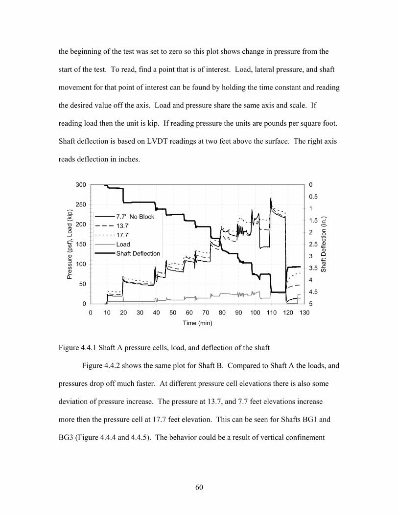
and Shaft BG3 at elevation 13.7 feet and 17.7 feet. Figure 4.4.1 shows a plot of Shaft
A’s three pressure cells, the load on that shaft, and the shaft deflection. The pressure at
60
the beginning of the test was set to zero so this plot shows change in pressure from the
start of the test. To read, find a point that is of interest. Load, lateral pressure, and shaft
movement for that point of interest can be found by holding the time constant and reading
the desired value off the axis. Load and pressure share the same axis and scale. If
reading load then the unit is kip. If reading pressure the units are pounds per square foot.
Shaft deflection is based on LVDT readings at two feet above the surface. The right axis
reads deflection in inches.
0
50
100
150
200
250
300
0 10 20 30 40 50 60 70 80 90 100 110 120 130
Time (min)
Pre
ssur
e (p
sf),
Load
(kip
)
0
0.5
1
1.5
2
2.5
3
3.5
4
4.5
5
Sha
ft D
efle
ctio
n (in
.)7.7' No Block13.7'17.7'LoadShaft Deflection
Figure 4.4.1 Shaft A pressure cells, load, and deflection of the shaft
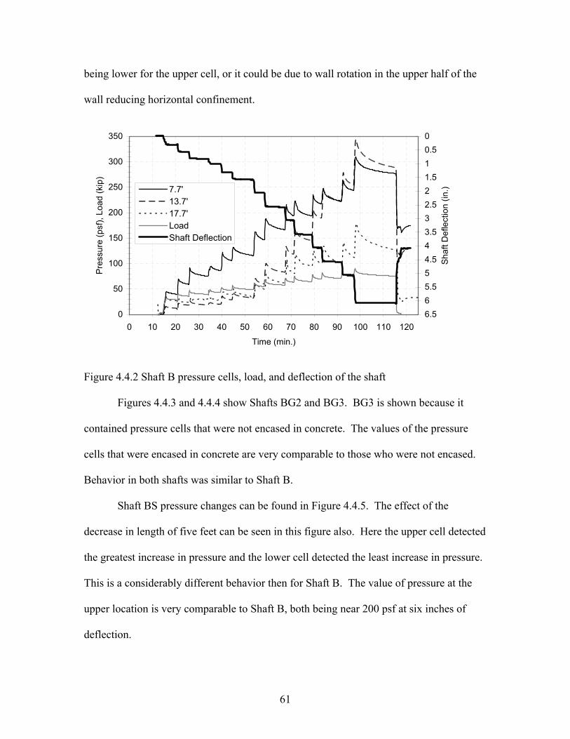
Figure 4.4.2 shows the same plot for Shaft B. Compared to Shaft A the loads, and
pressures drop off much faster. At different pressure cell elevations there is also some
deviation of pressure increase. The pressure at 13.7, and 7.7 feet elevations increase
more then the pressure cell at 17.7 feet elevation. This can be seen for Shafts BG1 and
BG3 (Figure 4.4.4 and 4.4.5). The behavior could be a result of vertical confinement
61
being lower for the upper cell, or it could be due to wall rotation in the upper half of the
wall reducing horizontal confinement.
0
50
100
150
200
250
300
350
0 10 20 30 40 50 60 70 80 90 100 110 120
Time (min.)
Pres
sure
(psf
), Lo
ad (k
ip)
00.511.522.533.544.555.566.5
Shaf
t Def
lect
ion
(in.)7.7'
13.7'17.7'LoadShaft Deflection
Figure 4.4.2 Shaft B pressure cells, load, and deflection of the shaft
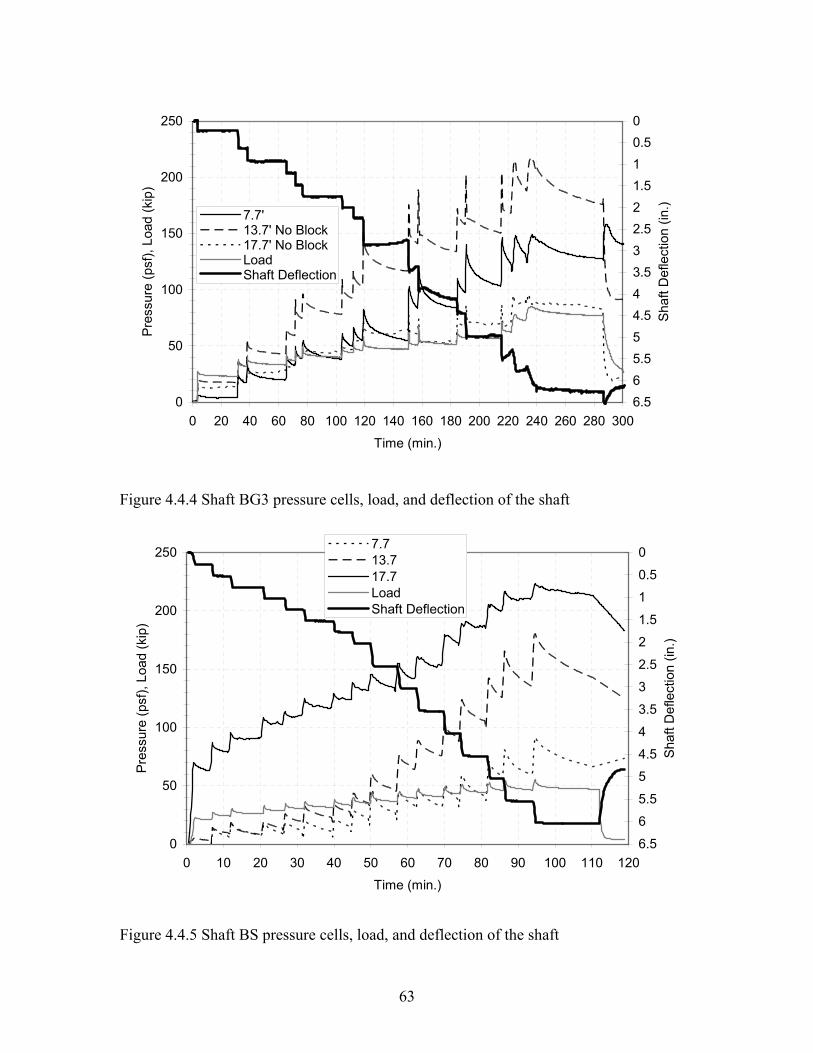
Figures 4.4.3 and 4.4.4 show Shafts BG2 and BG3. BG3 is shown because it
contained pressure cells that were not encased in concrete. The values of the pressure
cells that were encased in concrete are very comparable to those who were not encased.
Behavior in both shafts was similar to Shaft B.
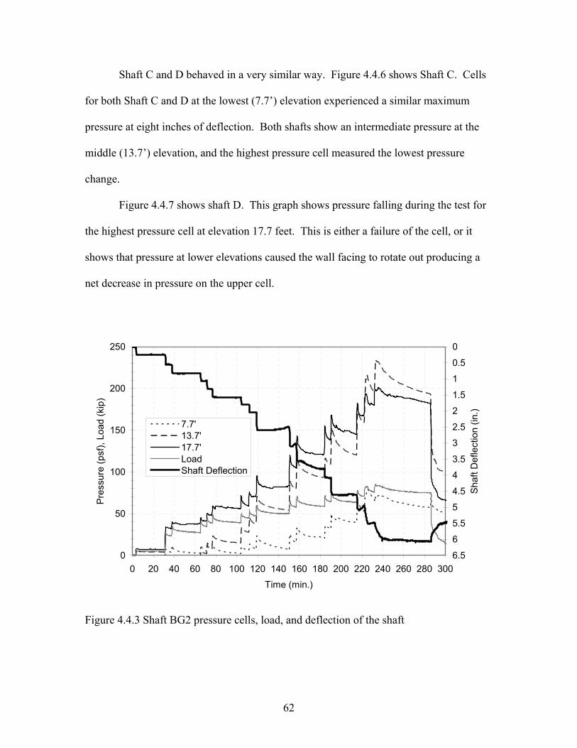
Shaft BS pressure changes can be found in Figure 4.4.5. The effect of the
decrease in length of five feet can be seen in this figure also. Here the upper cell detected
the greatest increase in pressure and the lower cell detected the least increase in pressure.
This is a considerably different behavior then for Shaft B. The value of pressure at the
upper location is very comparable to Shaft B, both being near 200 psf at six inches of
deflection.
62
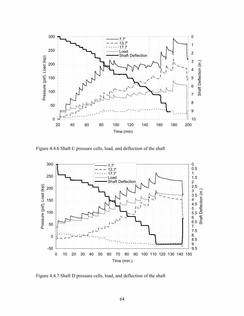
Shaft C and D behaved in a very similar way. Figure 4.4.6 shows Shaft C. Cells
for both Shaft C and D at the lowest (7.7’) elevation experienced a similar maximum
pressure at eight inches of deflection. Both shafts show an intermediate pressure at the
middle (13.7’) elevation, and the highest pressure cell measured the lowest pressure
change.
Figure 4.4.7 shows shaft D. This graph shows pressure falling during the test for
the highest pressure cell at elevation 17.7 feet. This is either a failure of the cell, or it
shows that pressure at lower elevations caused the wall facing to rotate out producing a
net decrease in pressure on the upper cell.
0
50
100
150
200
250
0 20 40 60 80 100 120 140 160 180 200 220 240 260 280 300
Time (min.)
Pres
sure
(psf
), Lo
ad (k
ip)
0
0.5
1
1.5
2
2.5
3
3.5
4
4.5
5
5.5
6
6.5
Shaf
t Def
lect
ion
(in.)
7.7'13.7'17.7'LoadShaft Deflection
Figure 4.4.3 Shaft BG2 pressure cells, load, and deflection of the shaft
63
0
50
100
150
200
250
0 20 40 60 80 100 120 140 160 180 200 220 240 260 280 300
Time (min.)
Pres
sure
(psf
), Lo
ad (k
ip)
00.511.522.533.544.555.566.5
Shaf
t Def
lect
ion
(in.)
7.7'13.7' No Block17.7' No BlockLoadShaft Deflection
Figure 4.4.4 Shaft BG3 pressure cells, load, and deflection of the shaft
0
50
100
150
200
250
0 10 20 30 40 50 60 70 80 90 100 110 120
Time (min.)
Pres
sure
(psf
), Lo
ad (k
ip)
0
0.5
1
1.5
2
2.5
3
3.5
4
4.5
5
5.5
6
6.5
Shaf
t Def
lect
ion
(in.)
7.713.717.7LoadShaft Deflection
Figure 4.4.5 Shaft BS pressure cells, load, and deflection of the shaft
64
0
50
100
150
200
250
300
20 40 60 80 100 120 140 160 180 200
Time (min)
Pres
sure
(psf
), Lo
ad (k
ip)
0
1
2
3
4
5
6
7
8
9
10
Shaf
t Def
lect
ion
(in.)
7.7'13.7'17.7LoadShaft Deflection
Figure 4.4.6 Shaft C pressure cells, load, and deflection of the shaft
-50
0
50
100
150
200
250
300
0 10 20 30 40 50 60 70 80 90 100 110 120 130 140 150
Time (min.)
Pres
sure
(psf
), Lo
ad (k
ip)
00.511.522.533.544.555.566.577.588.599.5
Shaf
t Def
lect
ion
(in.)
7.7'13.7'17.7'LoadShaft Deflection
Figure 4.4.7 Shaft D pressure cells, load, and deflection of the shaft
65
4.5 Surface Observations
The topsoil cover was compacted and relatively dry at the time of testing. This
topsoil cracked during the testing process, and these cracks are documented in the next
pages. During testing all shafts had cracks form behind the shafts due to caving and from
the sides at a diagonal toward the wall facing as a result of shaft movement. Figure 4.5.1
shows typical cracks that formed directly behind each shaft. Figure 4.5.2 shows typical
cracks that formed at a diagonal to the sides of the shaft. During the group test a large
crack developed at a distance of between 13.5 feet and 14.5 feet from the back of the wall
that ran parallel to the wall face. This is the same location as the end of the reinforced
zone. It is believed this crack is a result of sliding of the geogrid toward the wall facing
due to failure in pullout (Figure 4.5.3).
After testing of the group was performed, a section of geogrid between two of the
shafts was exhumed (Figure 4.5.4). This geogrid was then measured for elongation of the
grid. The data from this is presented in Figure 4.5.5.
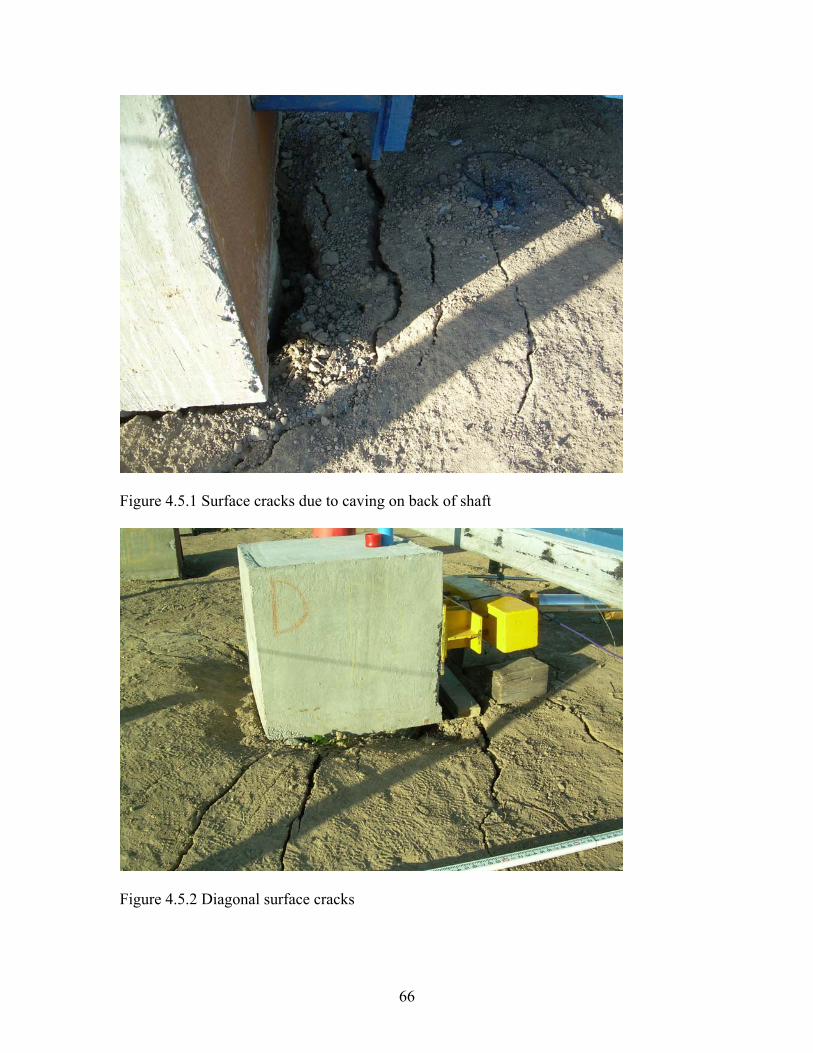
66
Figure 4.5.1 Surface cracks due to caving on back of shaft
Figure 4.5.2 Diagonal surface cracks
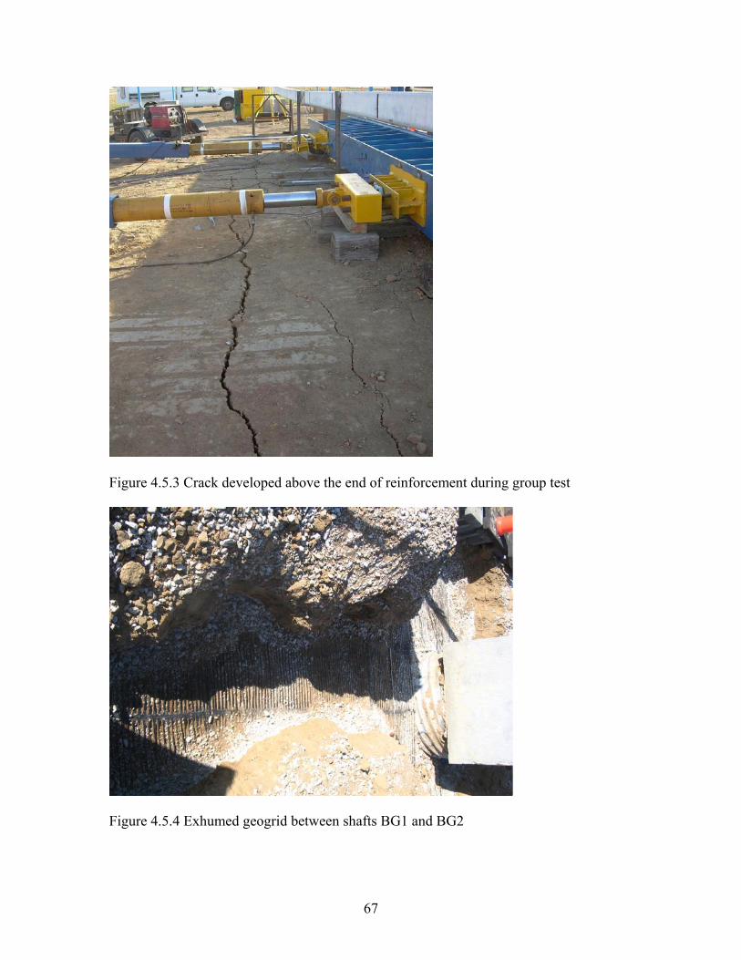
67
Figure 4.5.3 Crack developed above the end of reinforcement during group test
Figure 4.5.4 Exhumed geogrid between shafts BG1 and BG2
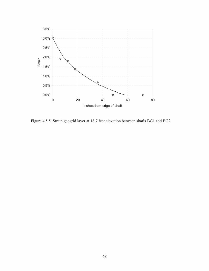
68
0.0%
0.5%
1.0%
1.5%
2.0%
2.5%
3.0%
3.5%
0 20 40 60 80
inches from edge of shaft
Str
ain
Figure 4.5.5 Strain geogrid layer at 18.7 feet elevation between shafts BG1 and BG2
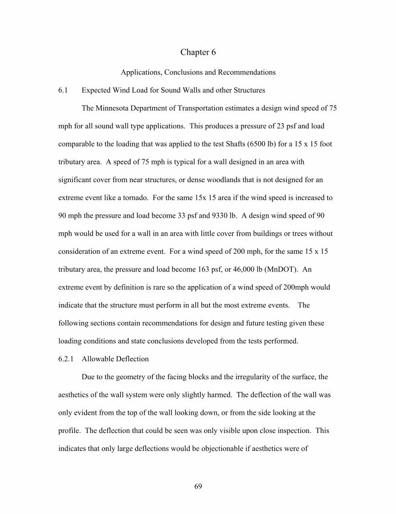
69
Chapter 6
Applications, Conclusions and Recommendations
6.1 Expected Wind Load for Sound Walls and other Structures
The Minnesota Department of Transportation estimates a design wind speed of 75
mph for all sound wall type applications. This produces a pressure of 23 psf and load
comparable to the loading that was applied to the test Shafts (6500 lb) for a 15 x 15 foot
tributary area. A speed of 75 mph is typical for a wall designed in an area with
significant cover from near structures, or dense woodlands that is not designed for an
extreme event like a tornado. For the same 15x 15 area if the wind speed is increased to
90 mph the pressure and load become 33 psf and 9330 lb. A design wind speed of 90
mph would be used for a wall in an area with little cover from buildings or trees without
consideration of an extreme event. For a wind speed of 200 mph, for the same 15 x 15
tributary area, the pressure and load become 163 psf, or 46,000 lb (MnDOT). An
extreme event by definition is rare so the application of a wind speed of 200mph would
indicate that the structure must perform in all but the most extreme events. The
following sections contain recommendations for design and future testing given these
loading conditions and state conclusions developed from the tests performed.
6.2.1 Allowable Deflection
Due to the geometry of the facing blocks and the irregularity of the surface, the
aesthetics of the wall system were only slightly harmed. The deflection of the wall was
only evident from the top of the wall looking down, or from the side looking at the
profile. The deflection that could be seen was only visible upon close inspection. This
indicates that only large deflections would be objectionable if aesthetics were of
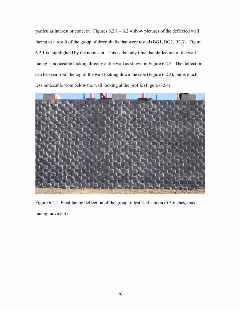
70
particular interest or concern. Figures 6.2.1 – 6.2.4 show pictures of the deflected wall
facing as a result of the group of three shafts that were tested (BG1, BG2, BG3). Figure
6.2.1 is highlighted by the noon sun. This is the only time that deflection of the wall
facing is noticeable looking directly at the wall as shown in Figure 6.2.2. The deflection
can be seen from the top of the wall looking down the side (Figure 6.2.3), but is much
less noticeable from below the wall looking at the profile (Figure 6.2.4).
Figure 6.2.1 Final facing deflection of the group of test shafts noon (5.3 inches, max
facing movment)
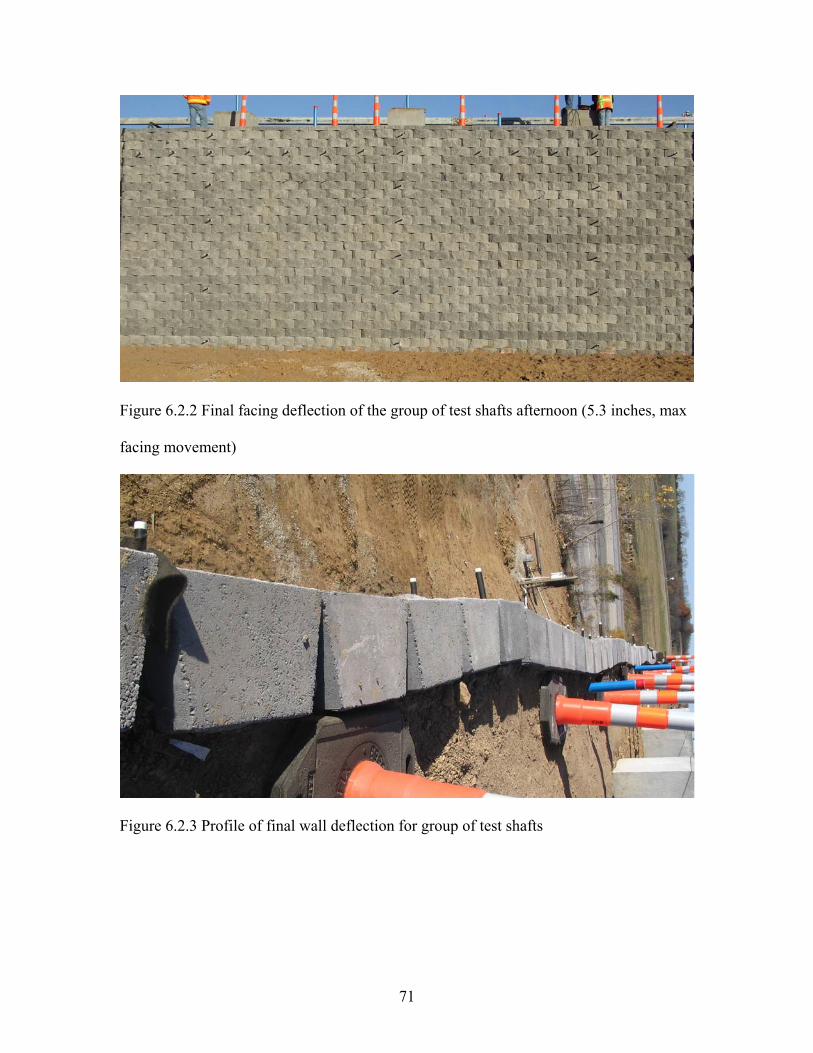
71
Figure 6.2.2 Final facing deflection of the group of test shafts afternoon (5.3 inches, max
facing movement)
Figure 6.2.3 Profile of final wall deflection for group of test shafts
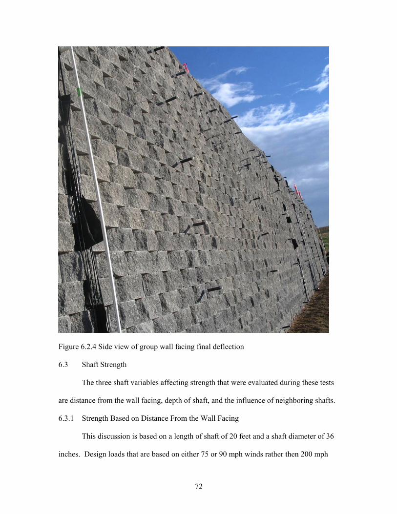
72
Figure 6.2.4 Side view of group wall facing final deflection
6.3 Shaft Strength
The three shaft variables affecting strength that were evaluated during these tests
are distance from the wall facing, depth of shaft, and the influence of neighboring shafts.
6.3.1 Strength Based on Distance From the Wall Facing
This discussion is based on a length of shaft of 20 feet and a shaft diameter of 36
inches. Design loads that are based on either 75 or 90 mph winds rather then 200 mph
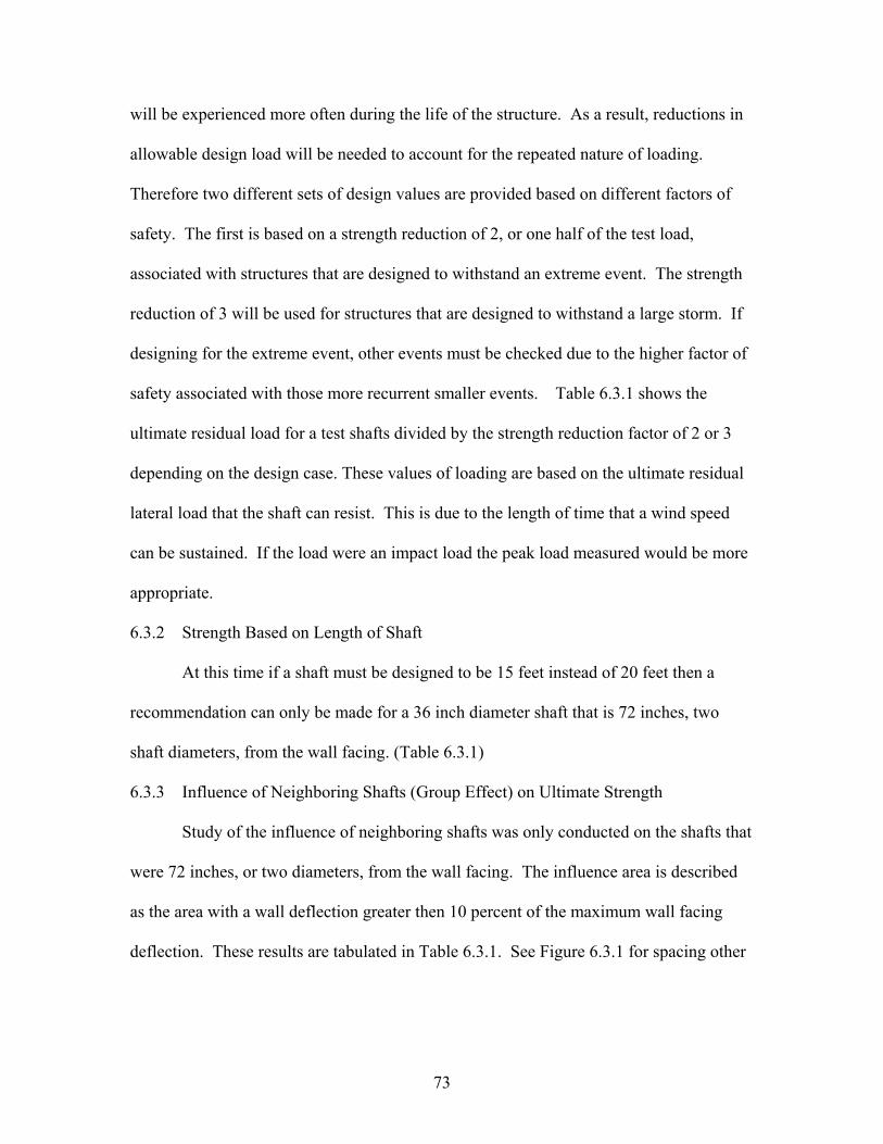
73
will be experienced more often during the life of the structure. As a result, reductions in
allowable design load will be needed to account for the repeated nature of loading.
Therefore two different sets of design values are provided based on different factors of
safety. The first is based on a strength reduction of 2, or one half of the test load,
associated with structures that are designed to withstand an extreme event. The strength
reduction of 3 will be used for structures that are designed to withstand a large storm. If
designing for the extreme event, other events must be checked due to the higher factor of
safety associated with those more recurrent smaller events. Table 6.3.1 shows the
ultimate residual load for a test shafts divided by the strength reduction factor of 2 or 3
depending on the design case. These values of loading are based on the ultimate residual
lateral load that the shaft can resist. This is due to the length of time that a wind speed
can be sustained. If the load were an impact load the peak load measured would be more
appropriate.
6.3.2 Strength Based on Length of Shaft
At this time if a shaft must be designed to be 15 feet instead of 20 feet then a
recommendation can only be made for a 36 inch diameter shaft that is 72 inches, two
shaft diameters, from the wall facing. (Table 6.3.1)
6.3.3 Influence of Neighboring Shafts (Group Effect) on Ultimate Strength
Study of the influence of neighboring shafts was only conducted on the shafts that
were 72 inches, or two diameters, from the wall facing. The influence area is described
as the area with a wall deflection greater then 10 percent of the maximum wall facing
deflection. These results are tabulated in Table 6.3.1. See Figure 6.3.1 for spacing other
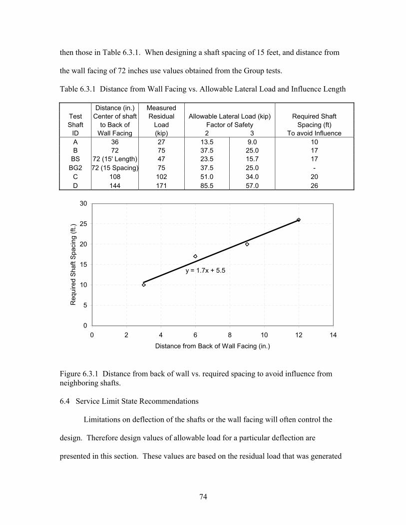
74
then those in Table 6.3.1. When designing a shaft spacing of 15 feet, and distance from
the wall facing of 72 inches use values obtained from the Group tests.
Table 6.3.1 Distance from Wall Facing vs. Allowable Lateral Load and Influence Length
Distance (in.) Measured Test Center of shaft Residual Allowable Lateral Load (kip) Required Shaft Shaft to Back of Load Factor of Safety Spacing (ft)
ID Wall Facing (kip) 2 3 To avoid Influence A 36 27 13.5 9.0 10 B 72 75 37.5 25.0 17
BS 72 (15' Length) 47 23.5 15.7 17 BG2 72 (15 Spacing) 75 37.5 25.0 -
C 108 102 51.0 34.0 20 D 144 171 85.5 57.0 26
y = 1.7x + 5.5
0
5
10
15
20
25
30
0 2 4 6 8 10 12 14
Distance from Back of Wall Facing (in.)
Req
uire
d Sh
aft S
paci
ng (f
t.)
Figure 6.3.1 Distance from back of wall vs. required spacing to avoid influence from neighboring shafts. 6.4 Service Limit State Recommendations
Limitations on deflection of the shafts or the wall facing will often control the
design. Therefore design values of allowable load for a particular deflection are
presented in this section. These values are based on the residual load that was generated
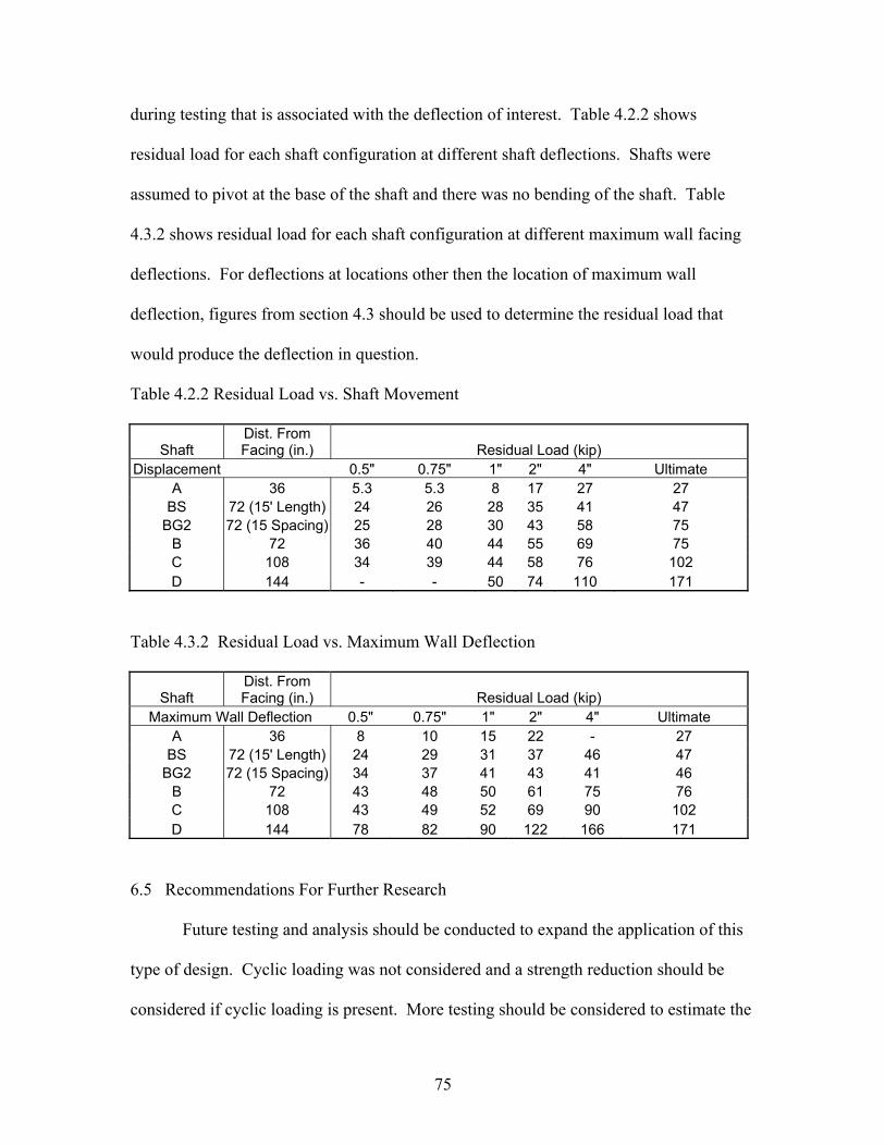
75
during testing that is associated with the deflection of interest. Table 4.2.2 shows
residual load for each shaft configuration at different shaft deflections. Shafts were
assumed to pivot at the base of the shaft and there was no bending of the shaft. Table
4.3.2 shows residual load for each shaft configuration at different maximum wall facing
deflections. For deflections at locations other then the location of maximum wall
deflection, figures from section 4.3 should be used to determine the residual load that
would produce the deflection in question.
Table 4.2.2 Residual Load vs. Shaft Movement
Shaft Dist. From Facing (in.) Residual Load (kip)
Displacement 0.5" 0.75" 1" 2" 4" Ultimate A 36 5.3 5.3 8 17 27 27
BS 72 (15' Length) 24 26 28 35 41 47 BG2 72 (15 Spacing) 25 28 30 43 58 75
B 72 36 40 44 55 69 75 C 108 34 39 44 58 76 102 D 144 - - 50 74 110 171
Table 4.3.2 Residual Load vs. Maximum Wall Deflection
Shaft Dist. From Facing (in.) Residual Load (kip)
Maximum Wall Deflection 0.5" 0.75" 1" 2" 4" Ultimate A 36 8 10 15 22 - 27
BS 72 (15' Length) 24 29 31 37 46 47 BG2 72 (15 Spacing) 34 37 41 43 41 46
B 72 43 48 50 61 75 76 C 108 43 49 52 69 90 102 D 144 78 82 90 122 166 171
6.5 Recommendations For Further Research
Future testing and analysis should be conducted to expand the application of this
type of design. Cyclic loading was not considered and a strength reduction should be
considered if cyclic loading is present. More testing should be considered to estimate the

76
influence the effect of different backfill material, types of geogrid, facing type, and
different reinforcement geometries. The effect of different spacings could also be
evaluated for other shaft distances from the facing. Another option, in addition to full
scale testing, to determine these variables would be to use numerical modeling.
Modeling may be used to simulate the testing that was performed and then modified to
determine the effects of varying aspects of the design.
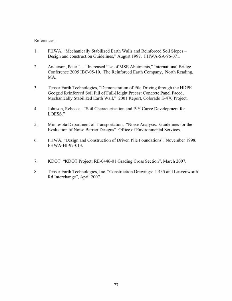
77
References: 1. FHWA, “Mechanically Stabilized Earth Walls and Reinforced Soil Slopes –
Design and construction Guidelines,” August 1997. FHWA-SA-96-071. 2. Anderson, Peter L., “Increased Use of MSE Abutments,” International Bridge
Conference 2005 IBC-05-10. The Reinforced Earth Company, North Reading, MA.
3. Tensar Earth Technologies, “Demonstration of Pile Driving through the HDPE
Geogrid Reinforced Soil Fill of Full-Height Precast Concrete Panel Faced, Mechanically Stabilized Earth Wall,” 2001 Report, Colorado E-470 Project.
4. Johnson, Rebecca, “Soil Characterization and P-Y Curve Development for
LOESS.” 5. Minnesota Department of Transportation, “Noise Analysis: Guidelines for the
Evaluation of Noise Barrier Designs” Office of Environmental Services. 6. FHWA, “Design and Construction of Driven Pile Foundations”, November 1998.
FHWA-HI-97-013. 7. KDOT “KDOT Project: RE-0446-01 Grading Cross Section”, March 2007. 8. Tensar Earth Technologies, Inc. “Construction Drawings: I-435 and Leavenworth
Rd Interchange”, April 2007.

78
Appendix
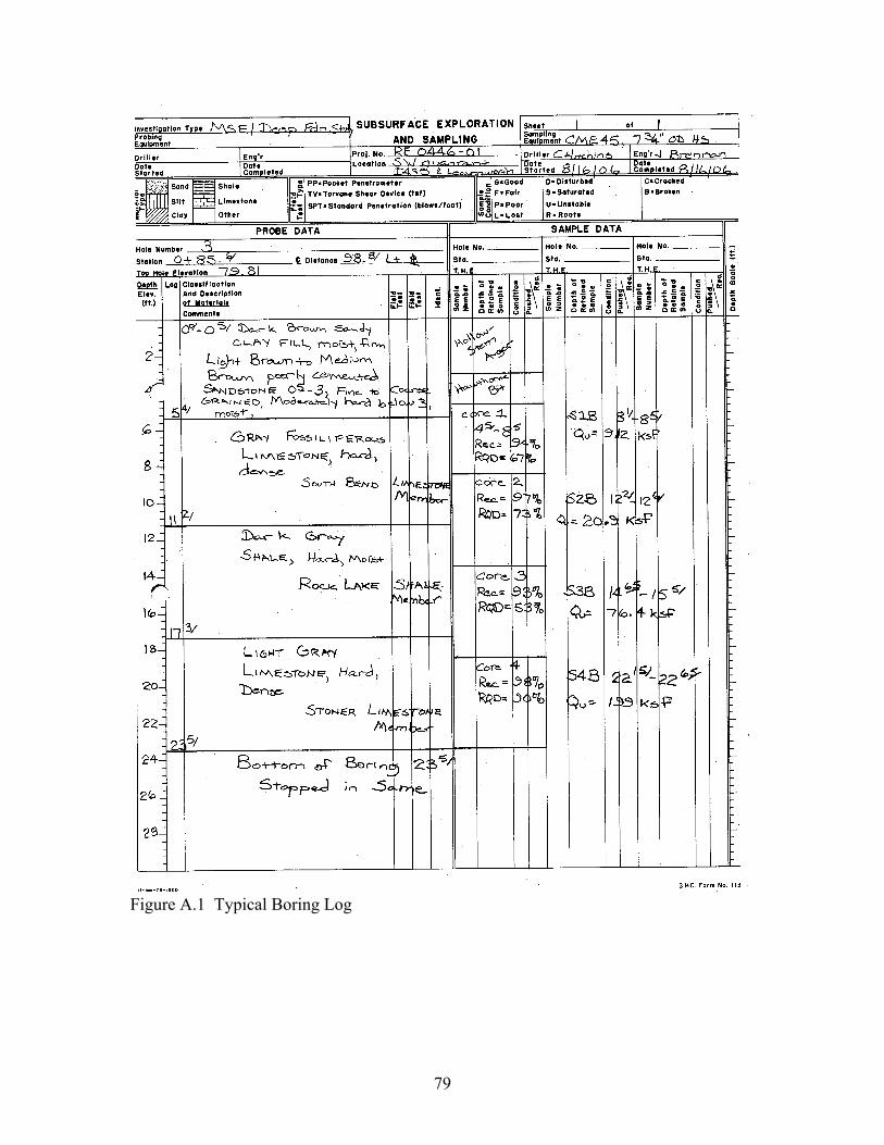
79
Figure A.1 Typical Boring Log
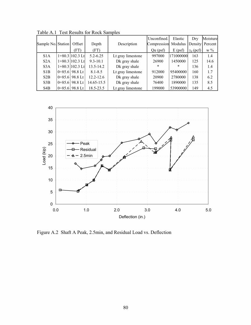
80
Table A.1 Test Results for Rock Samples Unconfined. Elastic Dry Moisture
Sample No. Station Offset Depth Description Compression Modulus Density Percent (FT) (FT) Qu (psf) E (psf) γd (pcf) w %
S1A 1+80.3 102.3 Lt 5.2-6.25 Lt gray limestone 997000 171000000 163 1.4 S2A 1+80.3 102.3 Lt 9.3-10.1 Dk gray shale 26900 1450000 125 14.6 S3A 1+80.3 102.3 Lt 13.5-14.2 Dk gray shale * * 136 1.4 S1B 0+85.6 98.8 Lt 8.1-8.5 Lt gray limestone 912000 95400000 160 1.7 S2B 0+85.6 98.8 Lt 12.2-12.6 Dk gray shale 20900 2780000 138 6.2 S3B 0+85.6 98.8 Lt 14.65-15.5 Dk gray shale 76400 1890000 135 8.5 S4B 0+85.6 98.8 Lt 18.5-23.5 Lt gray limestone 199000 53900000 149 4.5
0
5
10
15
20
25
30
35
40
0.0 1.0 2.0 3.0 4.0 5.0
Deflection (in.)
Load
(kip
)
PeakResidual2.5min
Figure A.2 Shaft A Peak, 2.5min, and Residual Load vs. Deflection
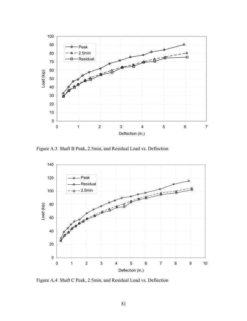
81
0
10
20
30
40
50
60
70
80
90
100
0 1 2 3 4 5 6 7
Deflection (in.)
Load
(kip
)Peak2.5minResidual
Figure A.3 Shaft B Peak, 2.5min, and Residual Load vs. Deflection
0
20
40
60
80
100
120
140
0 1 2 3 4 5 6 7 8 9 10
Deflection (in.)
Load
(kip
)
PeakResidual2.5min
Figure A.4 Shaft C Peak, 2.5min, and Residual Load vs. Deflection
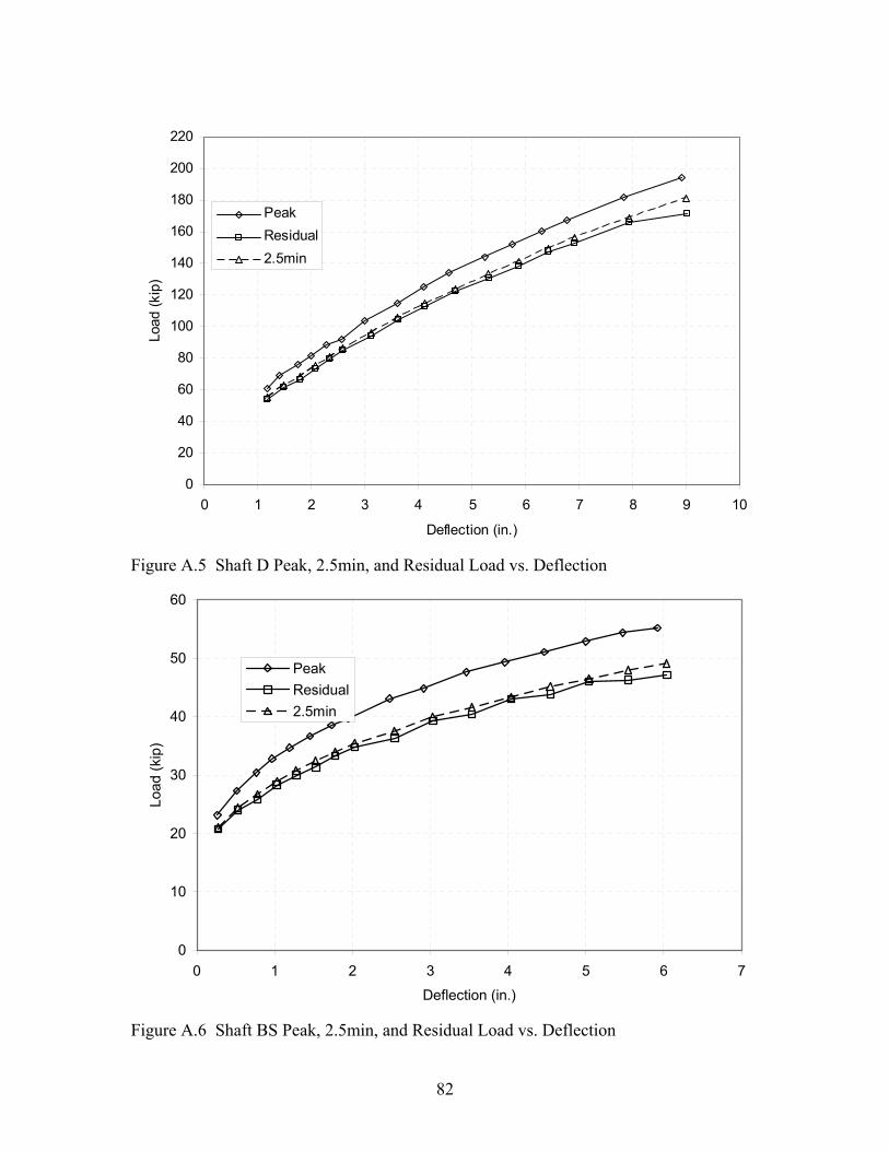
82
0
20
40
60
80
100
120
140
160
180
200
220
0 1 2 3 4 5 6 7 8 9 10
Deflection (in.)
Load
(kip
)
PeakResidual2.5min
Figure A.5 Shaft D Peak, 2.5min, and Residual Load vs. Deflection
0
10
20
30
40
50
60
0 1 2 3 4 5 6 7
Deflection (in.)
Load
(kip
)
PeakResidual2.5min
Figure A.6 Shaft BS Peak, 2.5min, and Residual Load vs. Deflection
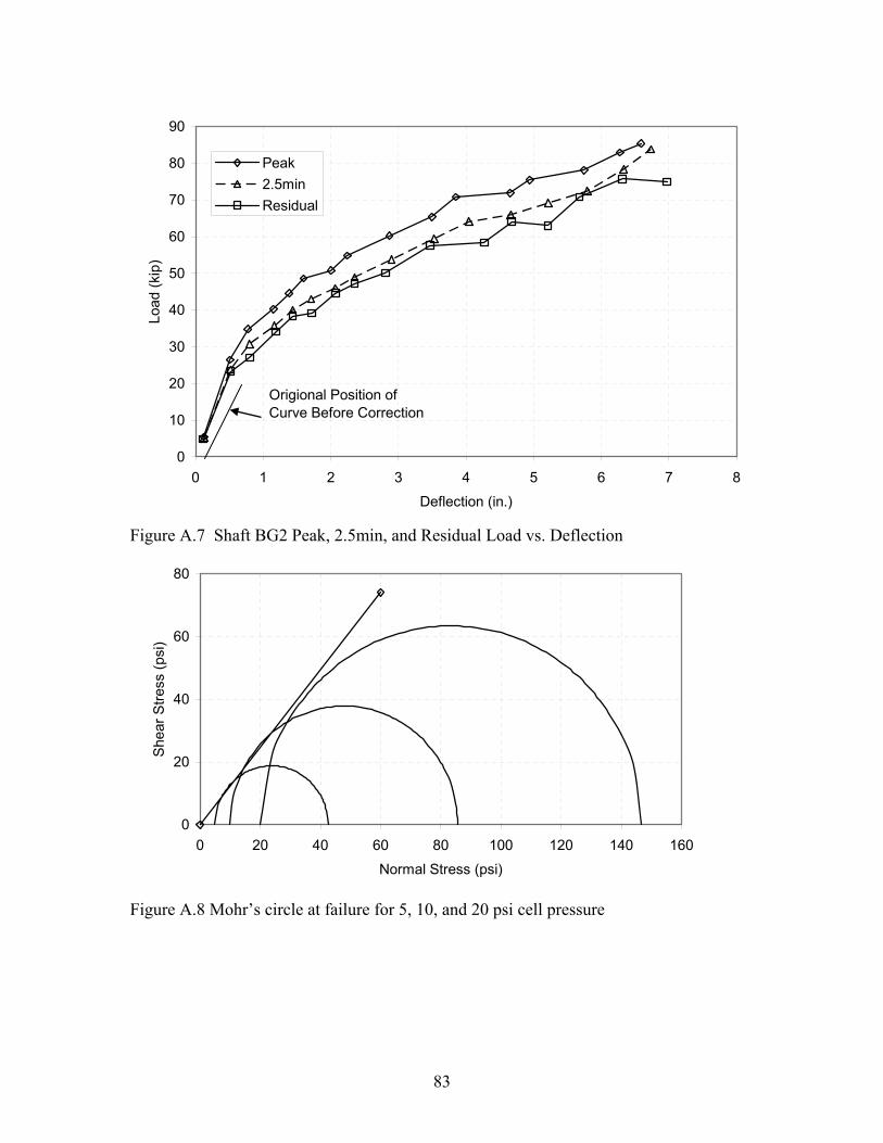
83
0
10
20
30
40
50
60
70
80
90
0 1 2 3 4 5 6 7 8
Deflection (in.)
Load
(kip
)Peak2.5minResidual
Origional Position of Curve Before Correction
Figure A.7 Shaft BG2 Peak, 2.5min, and Residual Load vs. Deflection
0
20
40
60
80
0 20 40 60 80 100 120 140 160
Normal Stress (psi)
Shea
r Stre
ss (p
si)
Figure A.8 Mohr’s circle at failure for 5, 10, and 20 psi cell pressure
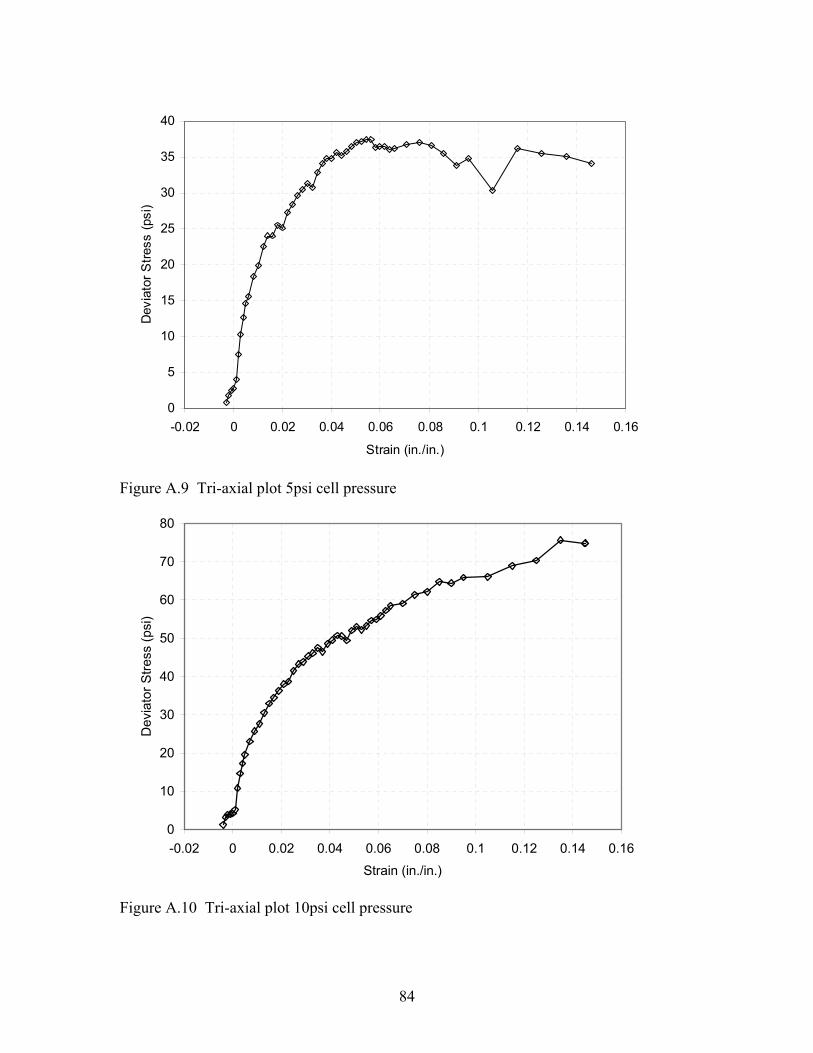
84
0
5
10
15
20
25
30
35
40
-0.02 0 0.02 0.04 0.06 0.08 0.1 0.12 0.14 0.16
Strain (in./in.)
Dev
iato
r Stre
ss (p
si)
Figure A.9 Tri-axial plot 5psi cell pressure
0
10
20
30
40
50
60
70
80
-0.02 0 0.02 0.04 0.06 0.08 0.1 0.12 0.14 0.16
Strain (in./in.)
Dev
iato
r Stre
ss (p
si)
Figure A.10 Tri-axial plot 10psi cell pressure
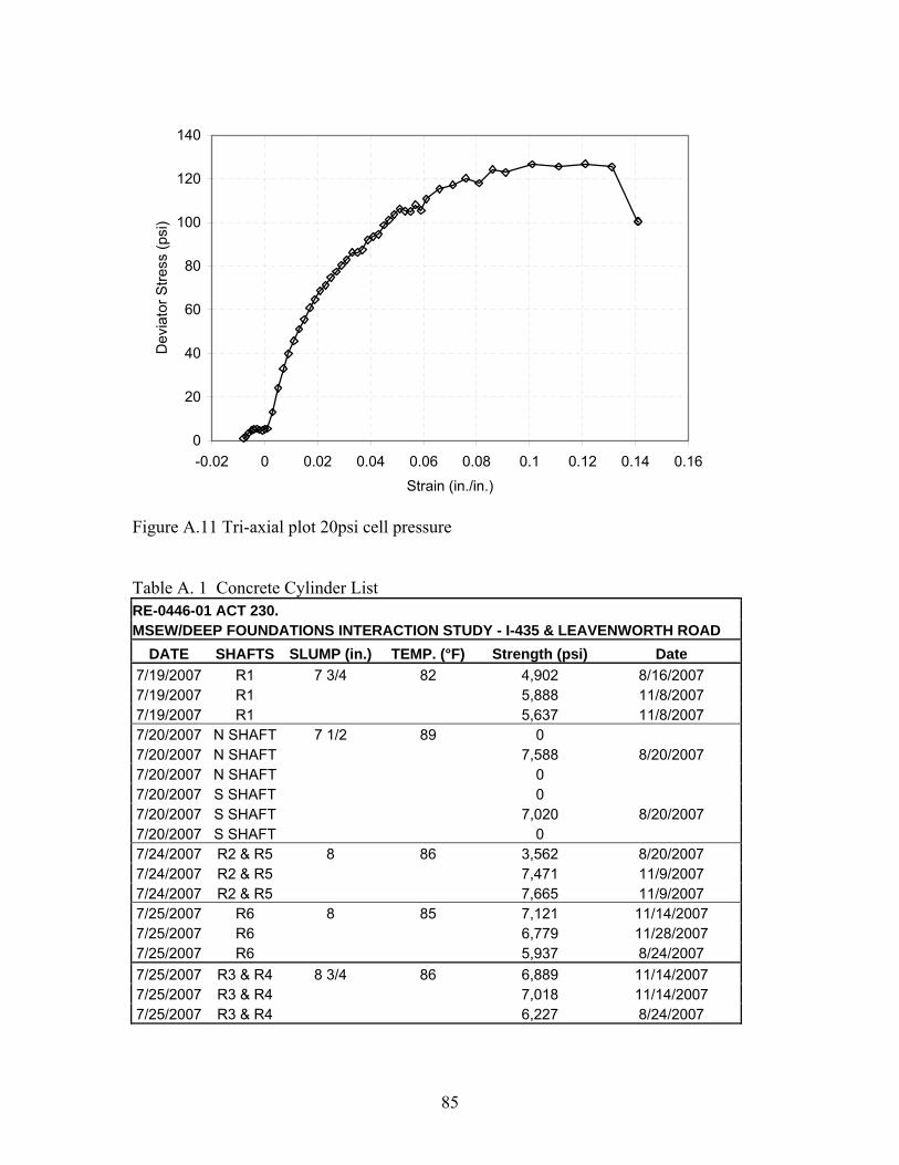
85
0
20
40
60
80
100
120
140
-0.02 0 0.02 0.04 0.06 0.08 0.1 0.12 0.14 0.16
Strain (in./in.)
Dev
iato
r Stre
ss (p
si)
Figure A.11 Tri-axial plot 20psi cell pressure Table A. 1 Concrete Cylinder List RE-0446-01 ACT 230. MSEW/DEEP FOUNDATIONS INTERACTION STUDY - I-435 & LEAVENWORTH ROAD
DATE SHAFTS SLUMP (in.) TEMP. (°F) Strength (psi) Date 7/19/2007 R1 7 3/4 82 4,902 8/16/2007 7/19/2007 R1 5,888 11/8/2007 7/19/2007 R1 5,637 11/8/2007 7/20/2007 N SHAFT 7 1/2 89 0 7/20/2007 N SHAFT 7,588 8/20/2007 7/20/2007 N SHAFT 0 7/20/2007 S SHAFT 0 7/20/2007 S SHAFT 7,020 8/20/2007 7/20/2007 S SHAFT 0 7/24/2007 R2 & R5 8 86 3,562 8/20/2007 7/24/2007 R2 & R5 7,471 11/9/2007 7/24/2007 R2 & R5 7,665 11/9/2007 7/25/2007 R6 8 85 7,121 11/14/2007 7/25/2007 R6 6,779 11/28/2007 7/25/2007 R6 5,937 8/24/2007 7/25/2007 R3 & R4 8 3/4 86 6,889 11/14/2007 7/25/2007 R3 & R4 7,018 11/14/2007 7/25/2007 R3 & R4 6,227 8/24/2007
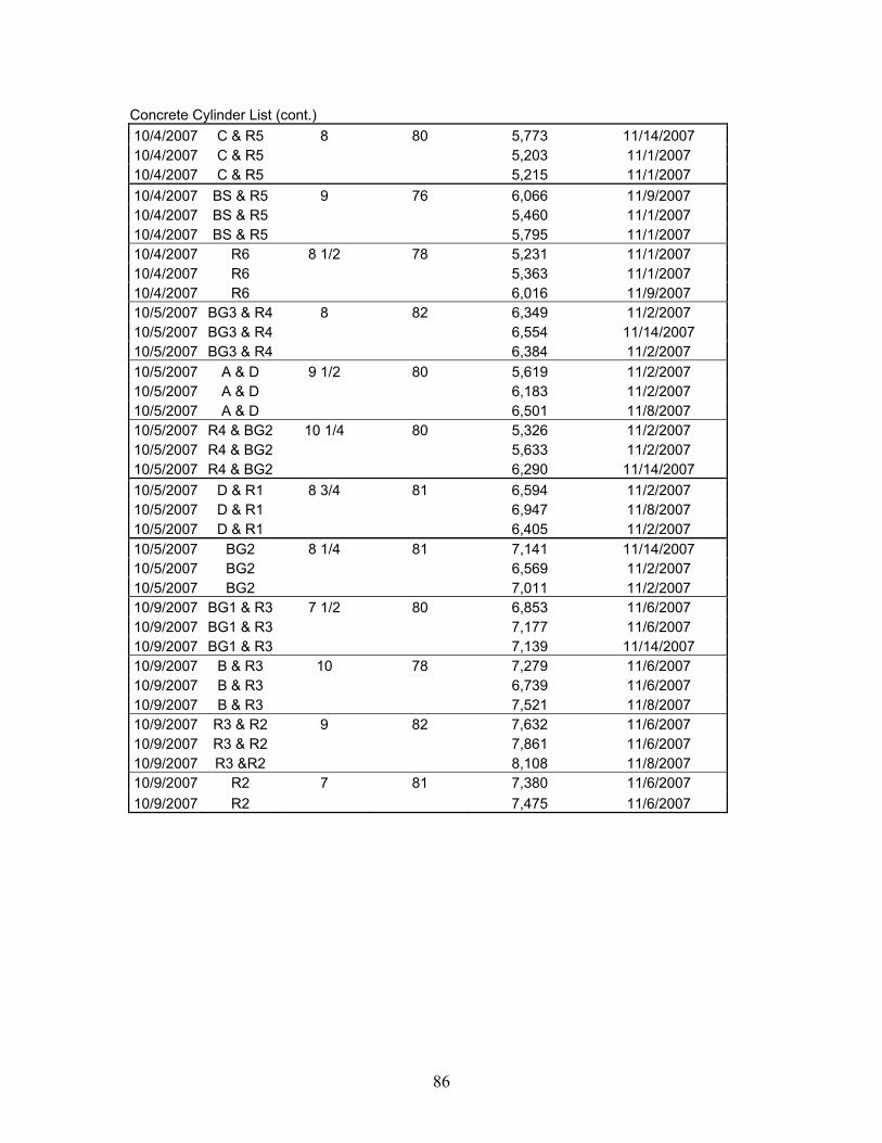
86
Concrete Cylinder List (cont.) 10/4/2007 C & R5 8 80 5,773 11/14/2007 10/4/2007 C & R5 5,203 11/1/2007 10/4/2007 C & R5 5,215 11/1/2007 10/4/2007 BS & R5 9 76 6,066 11/9/2007 10/4/2007 BS & R5 5,460 11/1/2007 10/4/2007 BS & R5 5,795 11/1/2007 10/4/2007 R6 8 1/2 78 5,231 11/1/2007 10/4/2007 R6 5,363 11/1/2007 10/4/2007 R6 6,016 11/9/2007 10/5/2007 BG3 & R4 8 82 6,349 11/2/2007 10/5/2007 BG3 & R4 6,554 11/14/2007 10/5/2007 BG3 & R4 6,384 11/2/2007 10/5/2007 A & D 9 1/2 80 5,619 11/2/2007 10/5/2007 A & D 6,183 11/2/2007 10/5/2007 A & D 6,501 11/8/2007 10/5/2007 R4 & BG2 10 1/4 80 5,326 11/2/2007 10/5/2007 R4 & BG2 5,633 11/2/2007 10/5/2007 R4 & BG2 6,290 11/14/2007 10/5/2007 D & R1 8 3/4 81 6,594 11/2/2007 10/5/2007 D & R1 6,947 11/8/2007 10/5/2007 D & R1 6,405 11/2/2007 10/5/2007 BG2 8 1/4 81 7,141 11/14/2007 10/5/2007 BG2 6,569 11/2/2007 10/5/2007 BG2 7,011 11/2/2007 10/9/2007 BG1 & R3 7 1/2 80 6,853 11/6/2007 10/9/2007 BG1 & R3 7,177 11/6/2007 10/9/2007 BG1 & R3 7,139 11/14/2007 10/9/2007 B & R3 10 78 7,279 11/6/2007 10/9/2007 B & R3 6,739 11/6/2007 10/9/2007 B & R3 7,521 11/8/2007 10/9/2007 R3 & R2 9 82 7,632 11/6/2007 10/9/2007 R3 & R2 7,861 11/6/2007 10/9/2007 R3 &R2 8,108 11/8/2007 10/9/2007 R2 7 81 7,380 11/6/2007 10/9/2007 R2 7,475 11/6/2007
Recommended