Faulting from First Principles
Gregory C. BerozaStanford University
2012 IRIS Workshop - Boise, Idaho - June 13-15
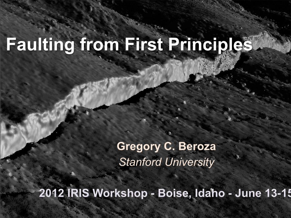
Earthquakes as slip on planar faults
(Beroza and Spudich, 1988)
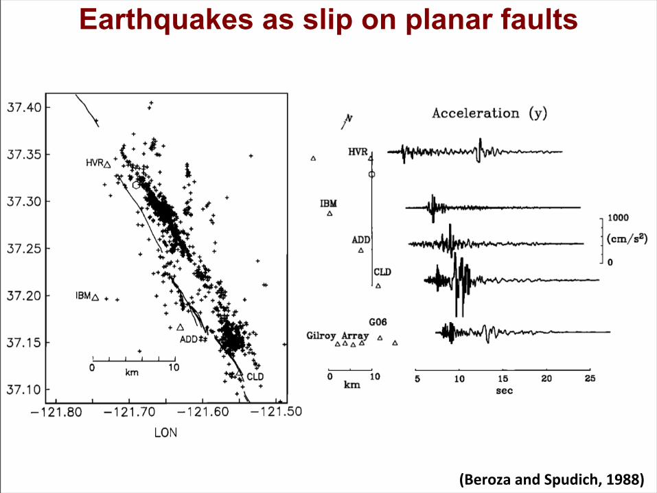
Earthquakes as slip on planar faults
(Beroza and Spudich, 1988)
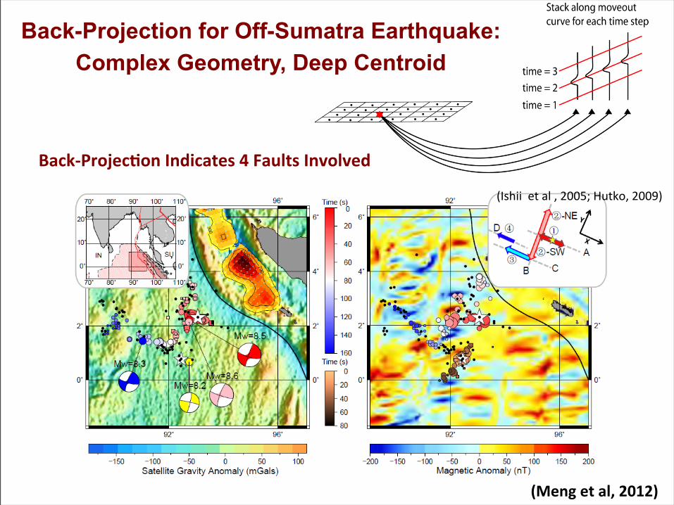
Back-Projection for Off-Sumatra Earthquake:Complex Geometry, Deep Centroid
Back-‐Projec+on Indicates 4 Faults Involved
(Ishii et al , 2005; Hutko, 2009)
(Meng et al, 2012)
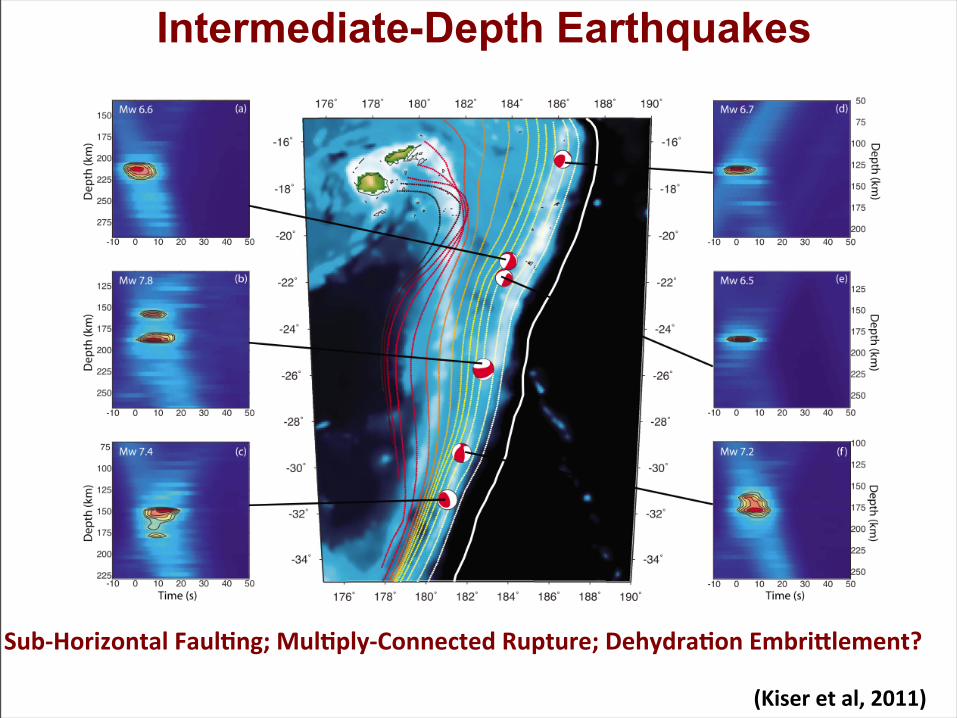
Intermediate-Depth Earthquakes
Sub-‐Horizontal Faul+ng; Mul+ply-‐Connected Rupture; Dehydra+on EmbriGlement?
(Kiser et al, 2011)
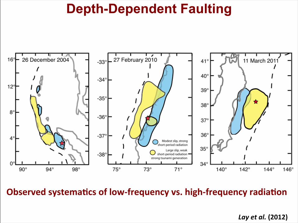
Depth-Dependent Faulting
Lay et al. (2012)
Observed systema+cs of low-‐frequency vs. high-‐frequency radia+on
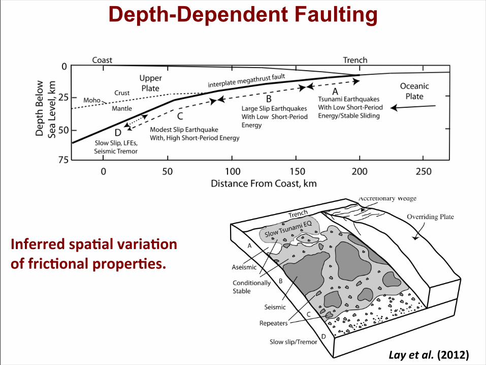
Depth-Dependent Faulting
Lay et al. (2012)
Inferred spa+al varia+on of fric+onal proper+es.
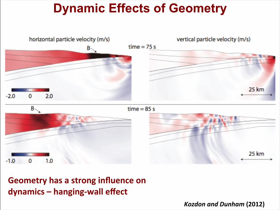
Dynamic Effects of Geometry
Kozdon and Dunham (2012)
Geometry has a strong influence on dynamics – hanging-‐wall effect
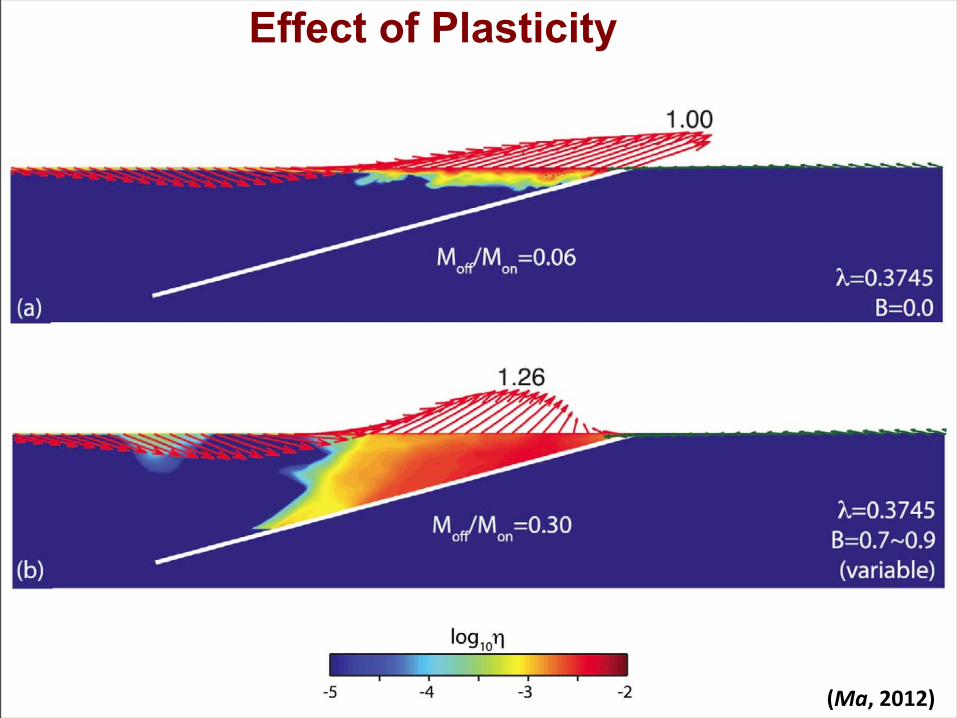
Effect of Plasticity
(Ma, 2012)
off-fault plastic strain
slip
velocity seismogram
fault friction
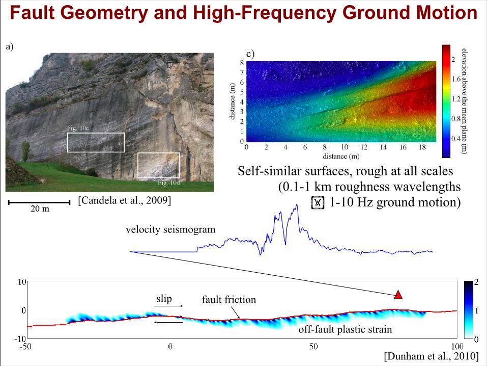
[Candela et al., 2009]
Self-similar surfaces, rough at all scales(0.1-1 km roughness wavelengths
1-10 Hz ground motion)
[Dunham et al., 2010]
Fault Geometry and High-Frequency Ground Motion
PGVPGA
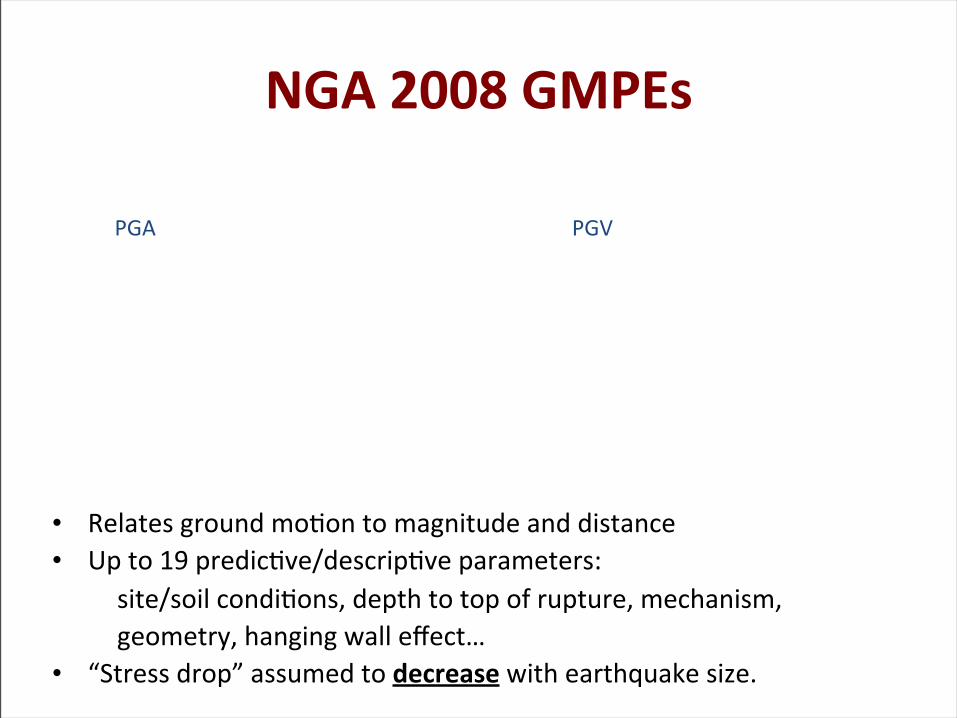
NGA 2008 GMPEs
• Relates ground mo/on to magnitude and distance• Up to 19 predic/ve/descrip/ve parameters: site/soil condi/ons, depth to top of rupture, mechanism, geometry, hanging wall effect…• “Stress drop” assumed to decrease with earthquake size.
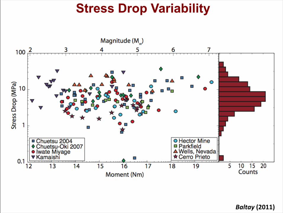
Stress Drop Variability
Baltay (2011)
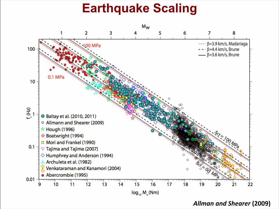
Earthquake Scaling
Allman and Shearer (2009)
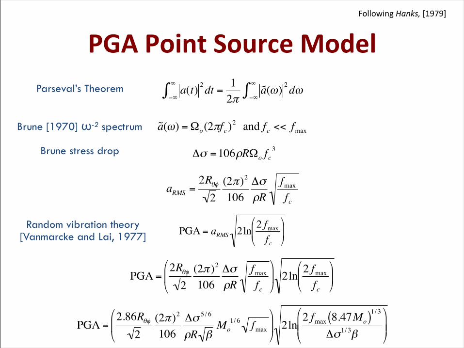
PGA Point Source Model
€
a(t) 2 dt−∞
∞
∫ =1
2π˜ a (ω) 2 dω
−∞
∞
∫
€
˜ a (ω) =Ωo(2πfc )2 and fc << fmax
Parseval’s Theorem
Following Hanks, [1979]
€
Δσ =106ρRΩo fc3Brune stress drop
€
aRMS =2Rθφ2(2π )2
106ΔσρR
fmaxfc
€
PGA = aRMS 2ln 2 fmaxfc
⎛
⎝ ⎜
⎞
⎠ ⎟
€
PGA =2Rθφ2(2π )2
106ΔσρR
fmaxfc
⎛
⎝ ⎜
⎞
⎠ ⎟ 2ln
2 fmaxfc
⎛
⎝ ⎜
⎞
⎠ ⎟
Random vibration theory[Vanmarcke and Lai, 1977]
Brune [1970] ω-2 spectrum
€
PGA =2.86Rθφ
2(2π )2
106Δσ 5 / 6
ρR βMo
1/ 6 fmax⎛
⎝ ⎜
⎞
⎠ ⎟ 2ln
2 fmax 8.47Mo( )1/ 3
Δσ1/ 3β
⎛
⎝ ⎜ ⎜
⎞
⎠ ⎟ ⎟
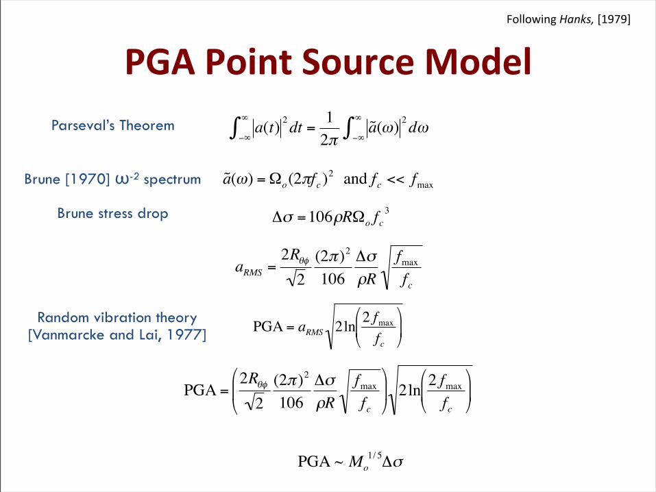
PGA Point Source Model
€
a(t) 2 dt−∞
∞
∫ =1
2π˜ a (ω) 2 dω
−∞
∞
∫
€
˜ a (ω) =Ωo(2πfc )2 and fc << fmax
Parseval’s Theorem
Following Hanks, [1979]
€
Δσ =106ρRΩo fc3Brune stress drop
€
aRMS =2Rθφ2(2π )2
106ΔσρR
fmaxfc
€
PGA = aRMS 2ln 2 fmaxfc
⎛
⎝ ⎜
⎞
⎠ ⎟
€
PGA =2Rθφ2(2π )2
106ΔσρR
fmaxfc
⎛
⎝ ⎜
⎞
⎠ ⎟ 2ln
2 fmaxfc
⎛
⎝ ⎜
⎞
⎠ ⎟
Random vibration theory[Vanmarcke and Lai, 1977]
Brune [1970] ω-2 spectrum
€
PGA ~ Mo1/ 5Δσ
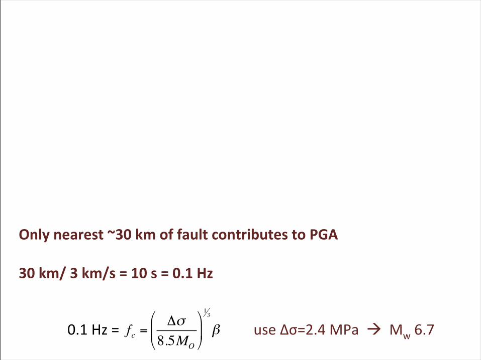
Only nearest ~30 km of fault contributes to PGA
30 km/ 3 km/s = 10 s = 0.1 Hz
€
fc =Δσ8.5MO
⎛
⎝ ⎜
⎞
⎠ ⎟
13
β0.1 Hz = use Δσ=2.4 MPa à Mw 6.7
• SaturaLon effect at M 6.7, consistent with NGA• Simple source models match GMPEs well
PGA Model
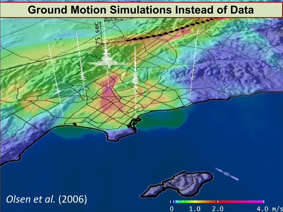
Olsen et al. (2006)
Ground Motion Simulations Instead of Data
Olsen et al. (2006)
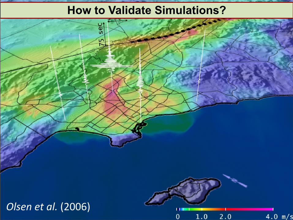
Ground Motion Simulations Instead of DataHow to Validate Simulations?
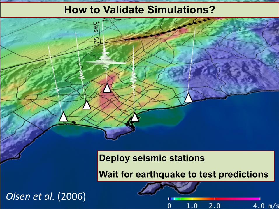
Olsen et al. (2006)
Deploy seismic stations
Wait for earthquake to test predictions
Ground Motion Simulations Instead of DataHow to Validate Simulations?
Olsen et al. (2006)
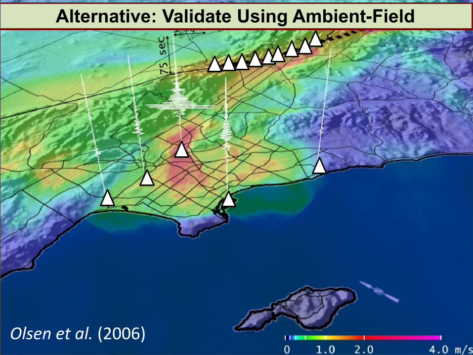
Ground Motion Simulations Instead of DataHow to Validate Simulations?Alternative: Validate Using Ambient-Field
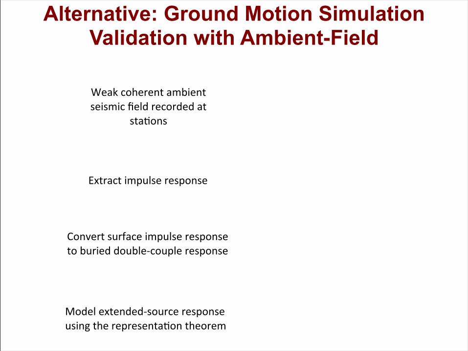
Extract impulse response
Model extended-‐source response using the representaLon theorem
Weak coherent ambient seismic field recorded at
staLons
Convert surface impulse responseto buried double-‐couple response
Alternative: Ground Motion Simulation Validation with Ambient-Field
Ambient Noise Impulse Responses vs. Earthquake
Depth and Mechanism Correc>ons Improve the Fit
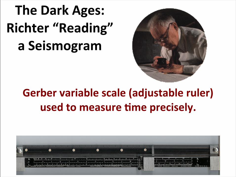
The Dark Ages: Richter “Reading” a Seismogram
Gerber variable scale (adjustable ruler) used to measure >me precisely.
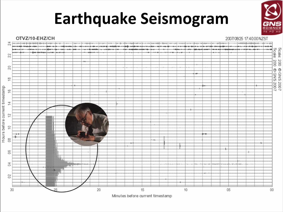
Earthquake Seismogram
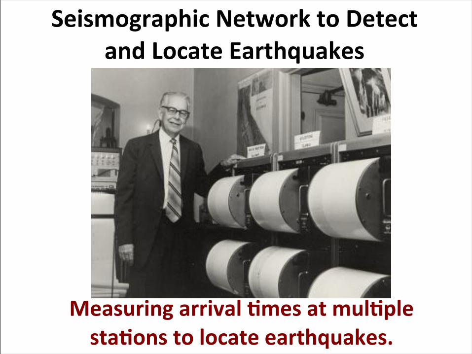
Seismographic Network to Detect and Locate Earthquakes
Measuring arrival >mes at mul>ple sta>ons to locate earthquakes.
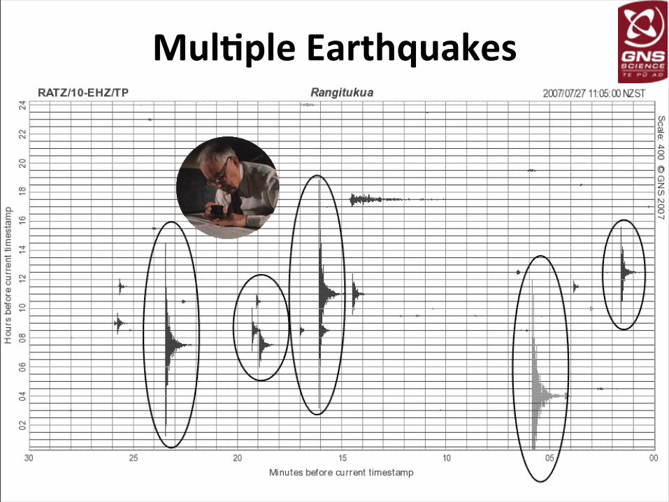
Mul+ple Earthquakes
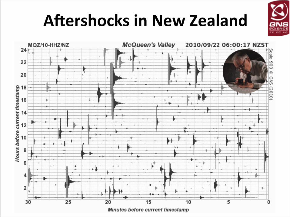
A`ershocks in New Zealand
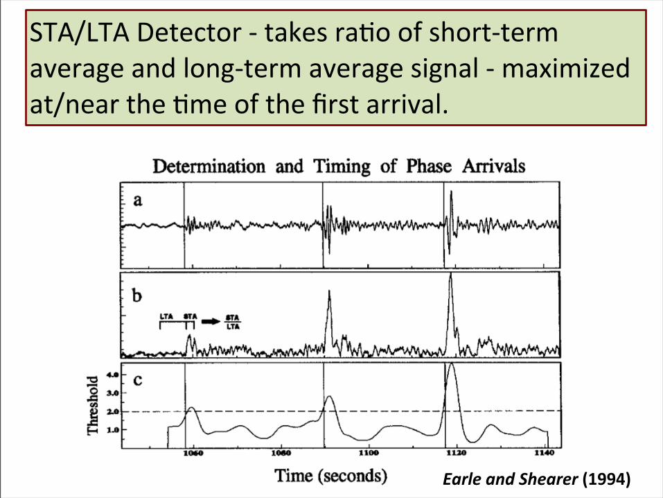
STA/LTA Detector -‐ takes raLo of short-‐term average and long-‐term average signal -‐ maximized at/near the Lme of the first arrival.
Earle and Shearer (1994)
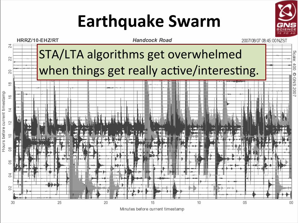
Earthquake Swarm
STA/LTA algorithms get overwhelmed when things get really acLve/interesLng.

The Cocktail Party Problem
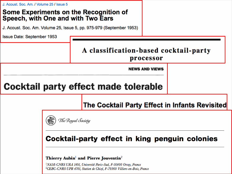
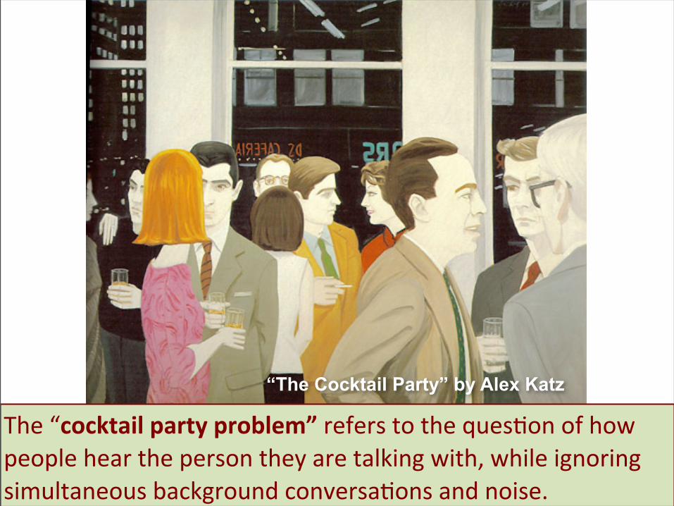
The “cocktail party problem” refers to the quesLon of how people hear the person they are talking with, while ignoring simultaneous background conversaLons and noise.
“The Cocktail Party” by Alex Katz
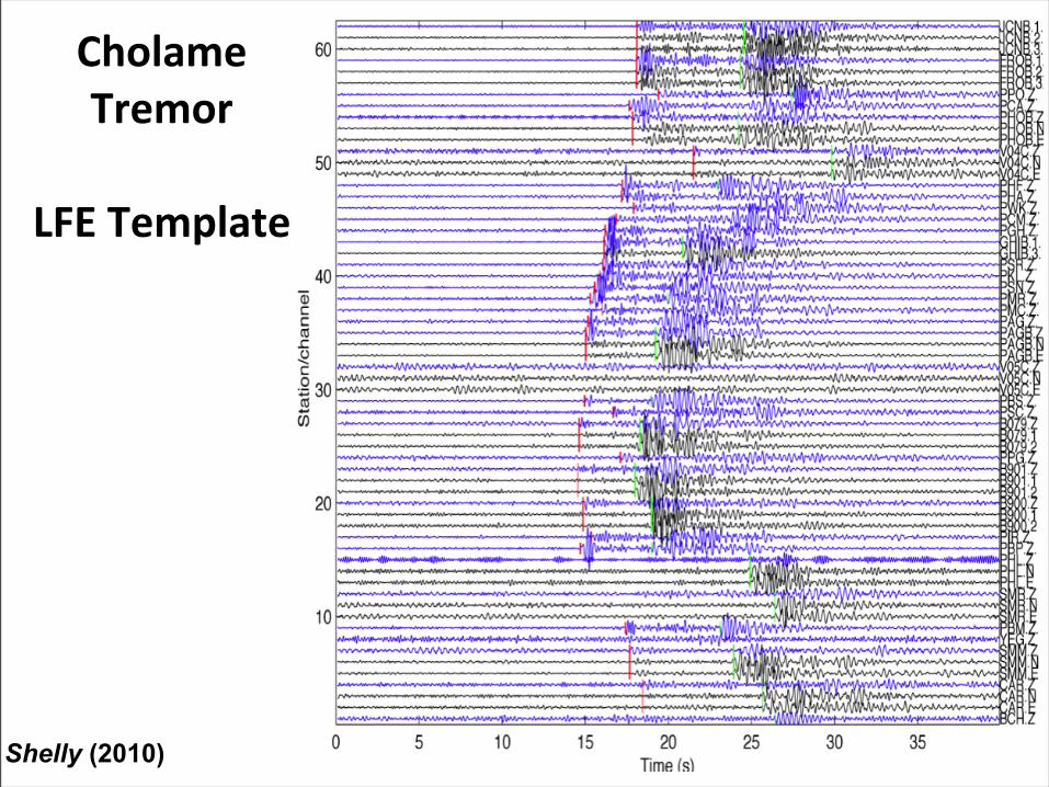
Cholame Tremor
LFE Template
Shelly (2010)
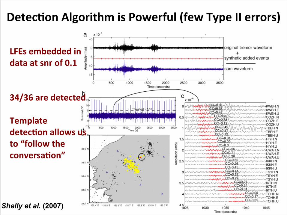
Detec>on Algorithm is Powerful (few Type II errors)
LFEs embedded in data at snr of 0.1
34/36 are detected
Template detec+on allows us to “follow the conversa+on”
Shelly et al. (2007)
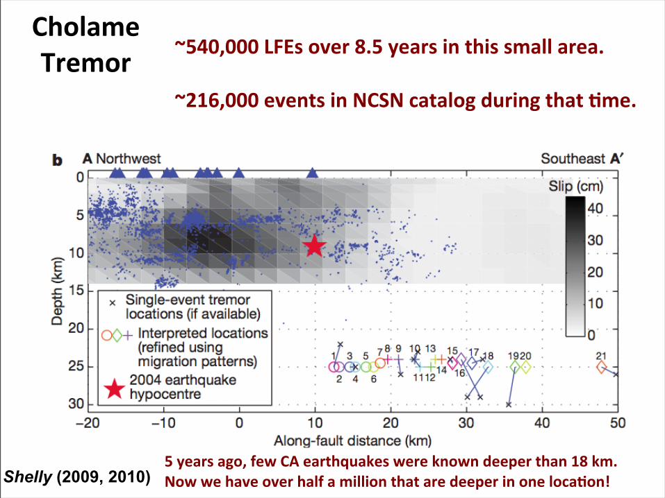
Cholame Tremor ~540,000 LFEs over 8.5 years in this small area.
~216,000 events in NCSN catalog during that +me.
Shelly (2009, 2010)5 years ago, few CA earthquakes were known deeper than 18 km.Now we have over half a million that are deeper in one locaJon!
Good luck Charlie!
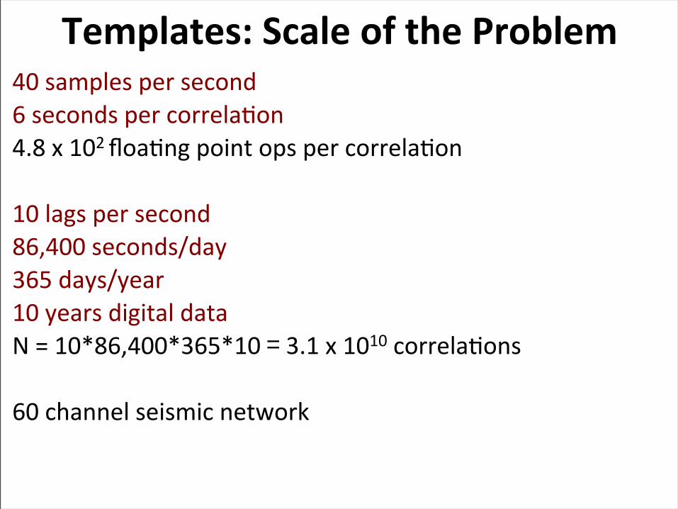
Templates: Scale of the Problem
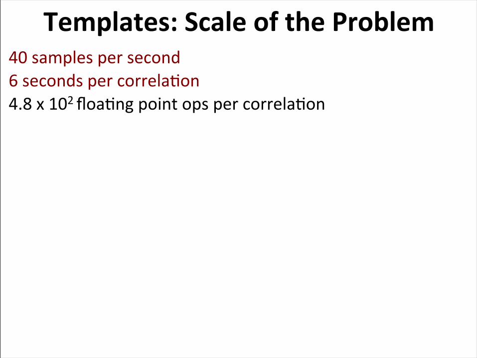
40 samples per second6 seconds per correlaLon4.8 x 102 floaLng point ops per correlaLon
Good luck Charlie!
Templates: Scale of the Problem
Good luck Charlie!
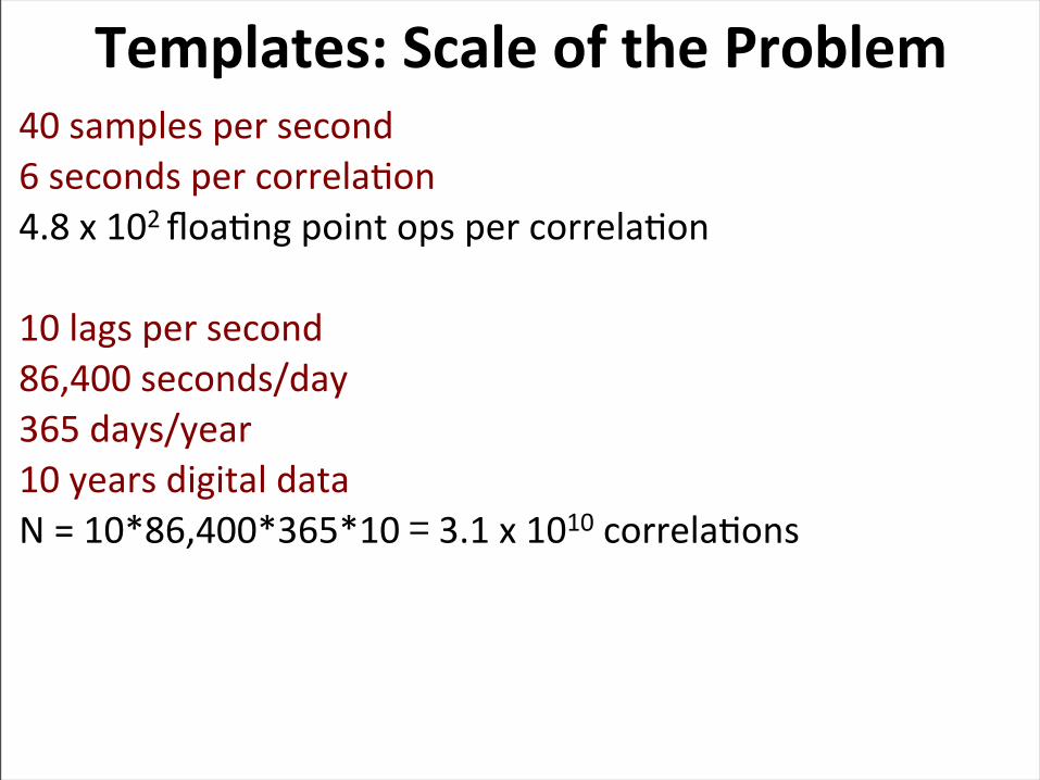
Templates: Scale of the Problem40 samples per second6 seconds per correlaLon4.8 x 102 floaLng point ops per correlaLon
10 lags per second86,400 seconds/day365 days/year10 years digital dataN = 10*86,400*365*10 = 3.1 x 10¹⁰ correlaLons
Good luck Charlie!
Templates: Scale of the Problem40 samples per second6 seconds per correlaLon4.8 x 102 floaLng point ops per correlaLon
10 lags per second86,400 seconds/day365 days/year10 years digital dataN = 10*86,400*365*10 = 3.1 x 10¹⁰ correlaLons
60 channel seismic network
Good luck Charlie!
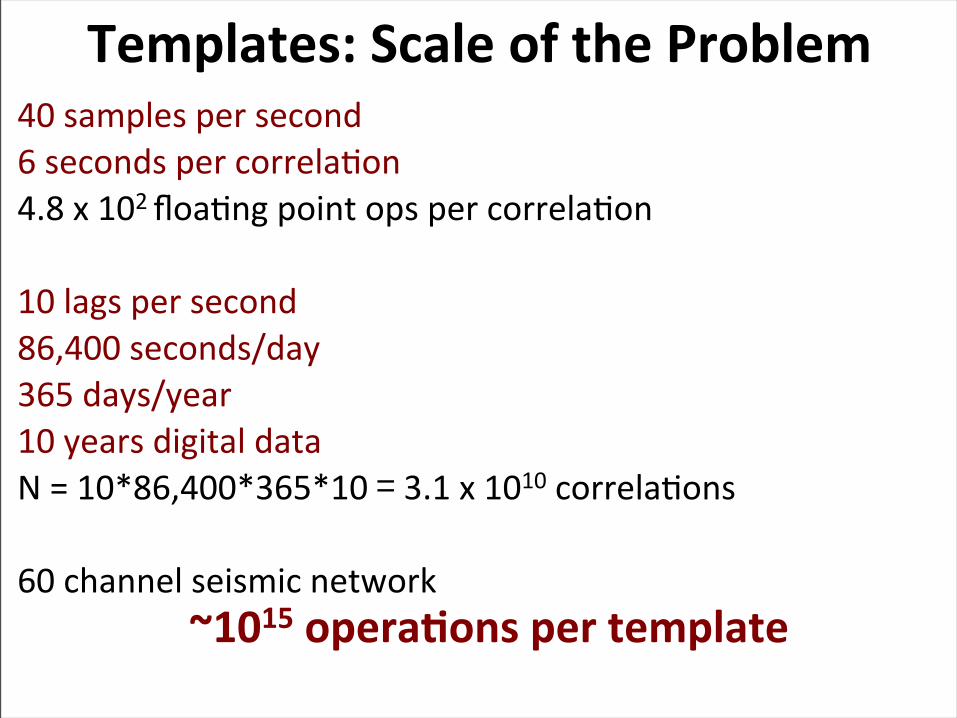
Templates: Scale of the Problem
~1015 opera>ons per template
40 samples per second6 seconds per correlaLon4.8 x 102 floaLng point ops per correlaLon
10 lags per second86,400 seconds/day365 days/year10 years digital dataN = 10*86,400*365*10 = 3.1 x 10¹⁰ correlaLons
60 channel seismic network
What if we don’t have a template?
Example of “Blind Source Separa>on” (knowledge of source is limited)
Can s>ll use no>on of looking for similar events across the network.
Compare everything with everything else.
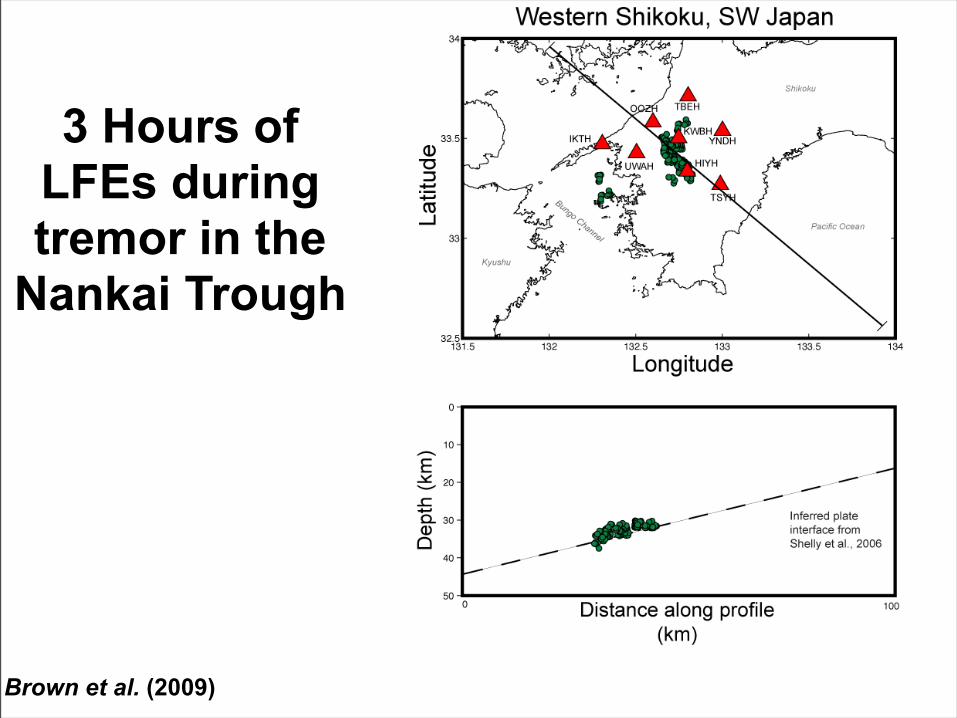
3 Hours of LFEs during tremor in the
Nankai Trough
Brown et al. (2009)
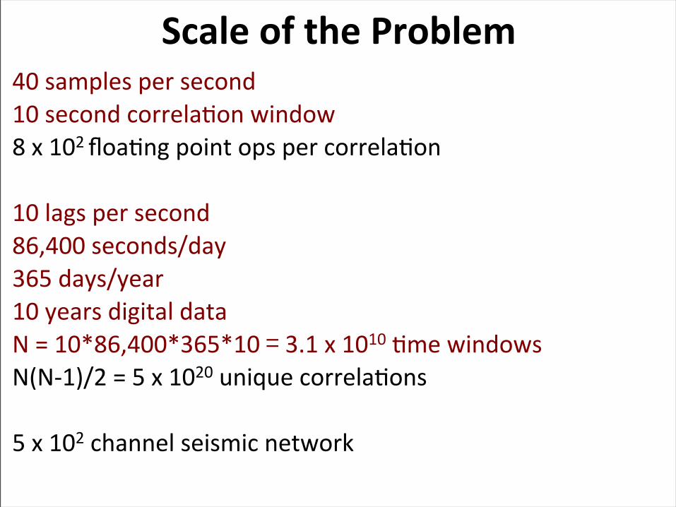
40 samples per second10 second correlaLon window8 x 102 floaLng point ops per correlaLon
10 lags per second86,400 seconds/day365 days/year10 years digital dataN = 10*86,400*365*10 = 3.1 x 10¹⁰ Lme windowsN(N-‐1)/2 = 5 x 10²⁰ unique correlaLons
5 x 10² channel seismic network
Scale of the Problem
40 samples per second10 second correlaLon window8 x 102 floaLng point ops per correlaLon
10 lags per second86,400 seconds/day365 days/year10 years digital dataN = 10*86,400*365*10 = 3.1 x 10¹⁰ Lme windowsN(N-‐1)/2 = 5 x 10²⁰ unique correlaLons
5 x 10² channel seismic network
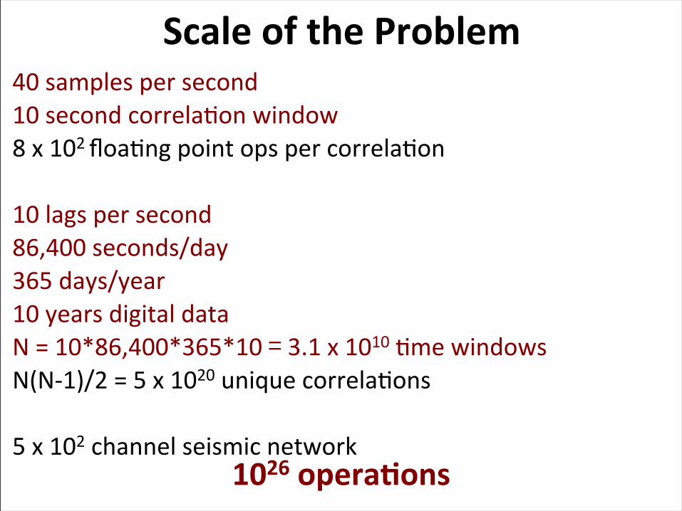
Scale of the Problem
1026 opera>ons
40 samples per second10 second correlaLon window8 x 102 floaLng point ops per correlaLon
10 lags per second86,400 seconds/day365 days/year10 years digital dataN = 10*86,400*365*10 = 3.1 x 10¹⁰ Lme windowsN(N-‐1)/2 = 5 x 10²⁰ unique correlaLons
5 x 10² channel seismic network
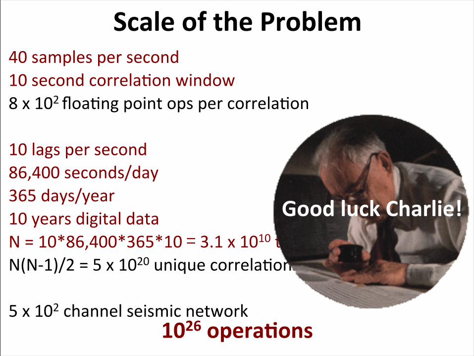
Good luck Charlie!
Scale of the Problem
1026 opera>ons
Being clever allows us to reduce by effort by orders of magnitude, but it’s s>ll computa>onally imposing.
We need to learn how to make lots of measurements(capacity) to exploit fully the wealth of data that new sensor technology will soon deliver.
Huge opportuni>es: earthquakes real-‐>me network seismology volcanoes geothermal shale gas other?
Scale/Poten+al of the Problem
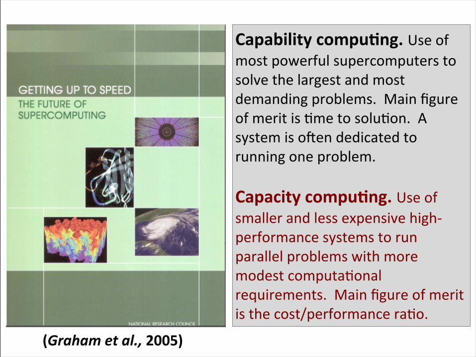
Capability compu>ng. Use of most powerful supercomputers to solve the largest and most demanding problems. Main figure of merit is Lme to soluLon. A system is ohen dedicated to running one problem.
Capacity compu>ng. Use of smaller and less expensive high-‐performance systems to run parallel problems with more modest computaLonal requirements. Main figure of merit is the cost/performance raLo.
(Graham et al., 2005)
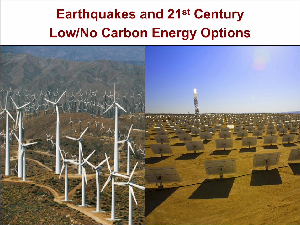
Earthquakes and 21st Century Low/No Carbon Energy Options
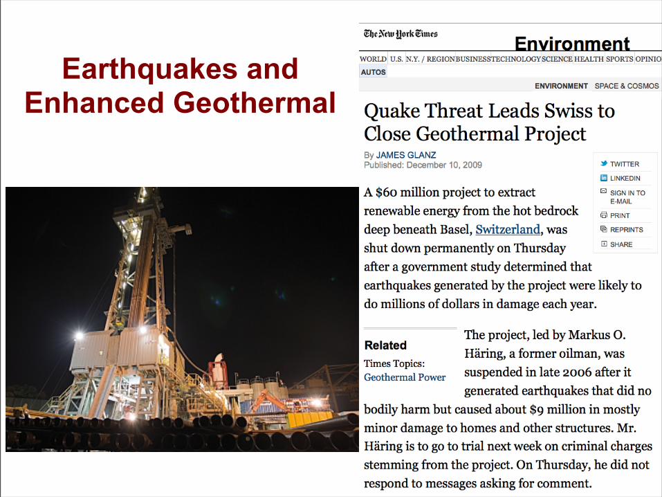
Earthquakes and Enhanced Geothermal
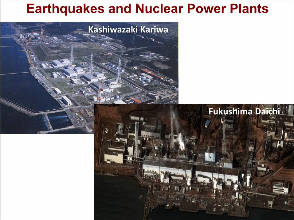
Earthquakes and Nuclear Power PlantsKashiwazaki Kariwa
Fukushima Daichi
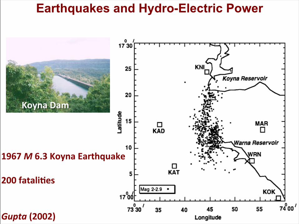
Earthquakes and Hydro-Electric Power
Koyna Dam
1967 M 6.3 Koyna Earthquake
200 fatali+es
Gupta (2002)
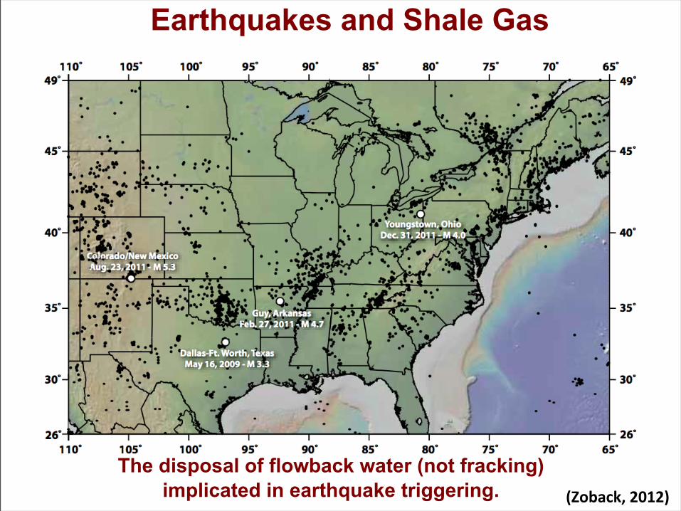
Earthquakes and Shale Gas
The disposal of flowback water (not fracking) implicated in earthquake triggering. (Zoback, 2012)
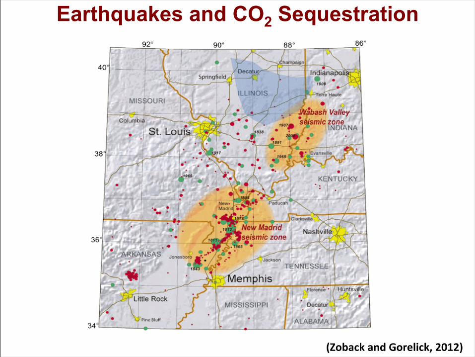
Earthquakes and CO2 Sequestration
(Zoback and Gorelick, 2012)
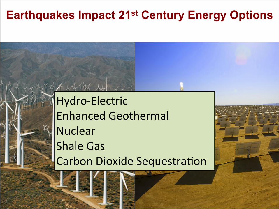
Earthquakes Impact 21st Century Energy Options
Hydro-‐Electric Enhanced Geothermal Nuclear Shale Gas Carbon Dioxide SequestraLon
Conclusions
• Seismology is cri>cal to the future of civiliza>on.
• We have a lot of data, we will soon have a lot more. We need to think hard about how to use it. Doing so will allow us to see earthquakes, and Earth structure, much more clearly. HPC will be an important part of this.
• It is the best of >mes… to be a seismologist.
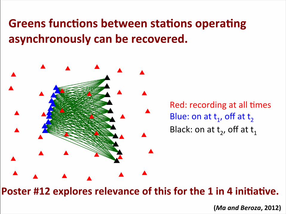
Greens func>ons between sta>ons opera>ng asynchronously can be recovered.
Red: recording at all LmesBlue: on at t1, off at t2Black: on at t2, off at t1
Poster #12 explores relevance of this for the 1 in 4 ini>a>ve.(Ma and Beroza, 2012)
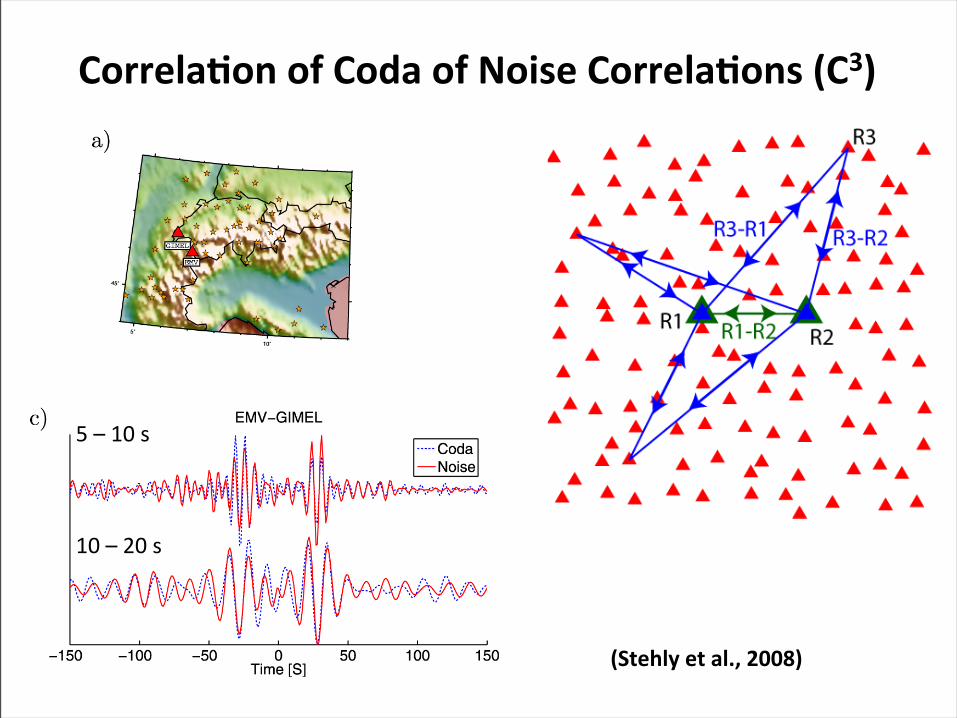
Correla>on of Coda of Noise Correla>ons (C3)
(Stehly et al., 2008)
5 – 10 s
10 – 20 s
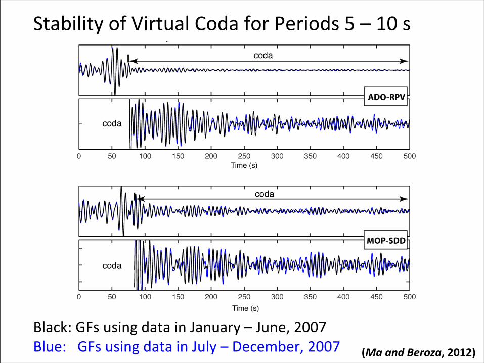
Stability of Virtual Coda for Periods 5 – 10 s
Black: GFs using data in January – June, 2007Blue: GFs using data in July – December, 2007 (Ma and Beroza, 2012)
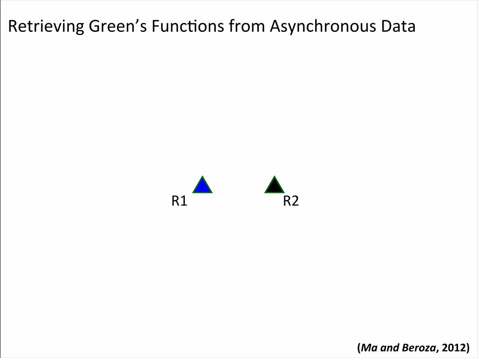
Retrieving Green’s FuncLons from Asynchronous Data
R1 R2
(Ma and Beroza, 2012)
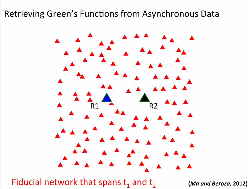
Retrieving Green’s FuncLons from Asynchronous Data
Fiducial network that spans t1 and t2
R1 R2
(Ma and Beroza, 2012)
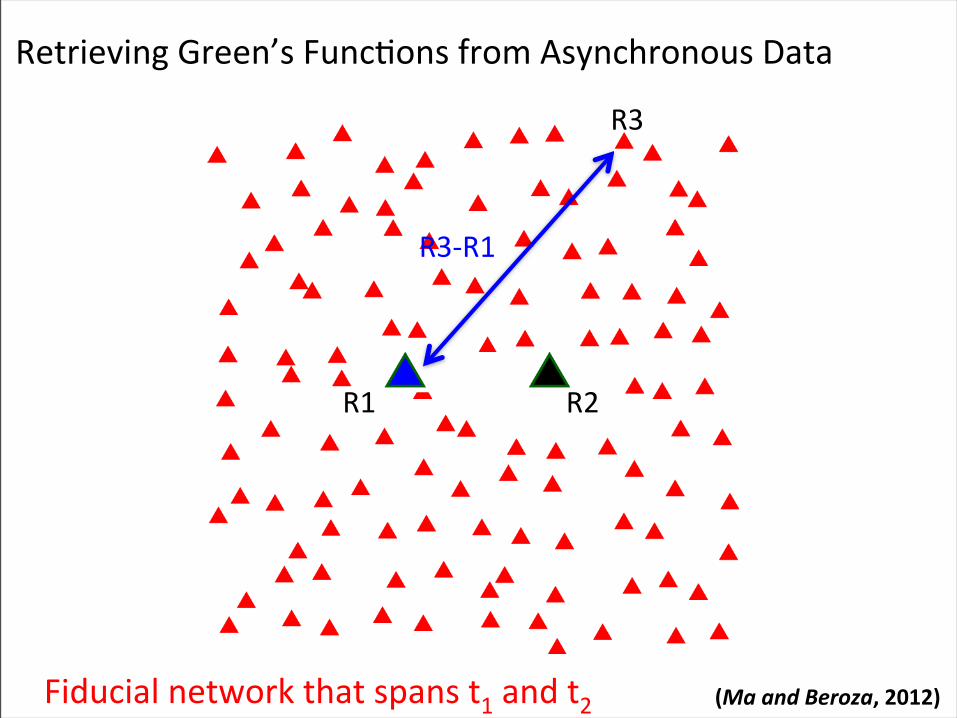
Retrieving Green’s FuncLons from Asynchronous Data
R3-‐R1
R3
Fiducial network that spans t1 and t2
R1 R2
(Ma and Beroza, 2012)
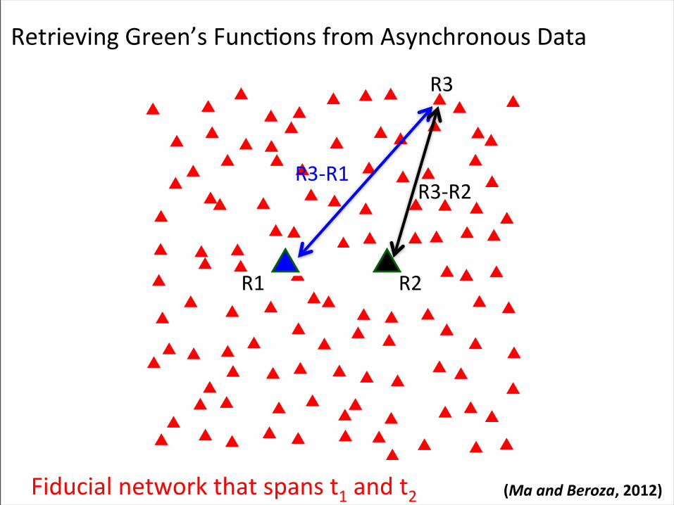
Retrieving Green’s FuncLons from Asynchronous Data
R3-‐R1R3-‐R2
R3
Fiducial network that spans t1 and t2
R1 R2
(Ma and Beroza, 2012)
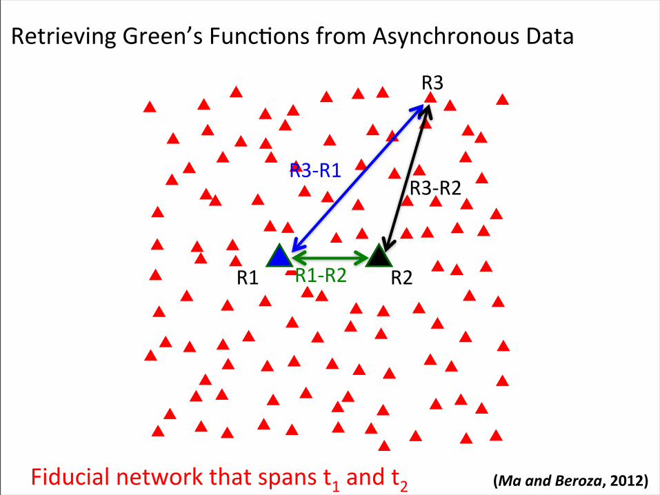
Retrieving Green’s FuncLons from Asynchronous Data
R1-‐R2
R3-‐R1R3-‐R2
R3
Fiducial network that spans t1 and t2
R1 R2
(Ma and Beroza, 2012)
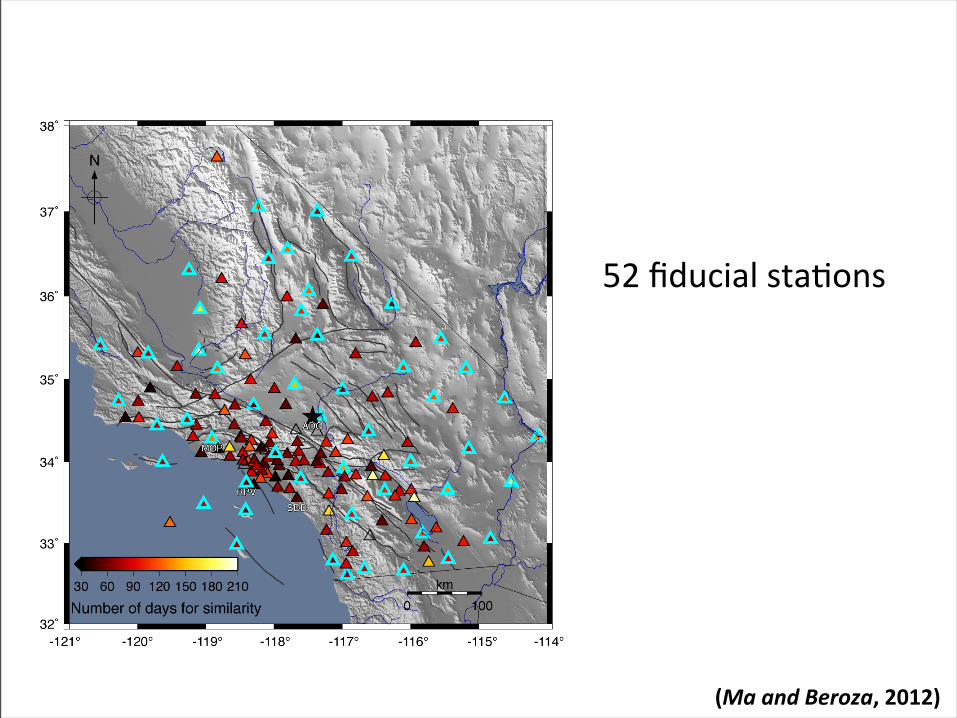
52 fiducial staLons
(Ma and Beroza, 2012)
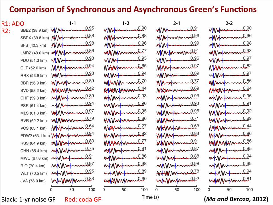
Comparison of Synchronous and Asynchronous Green’s Func+onsR1: ADOR2:
Black: 1-‐yr noise GF Red: coda GF (Ma and Beroza, 2012)
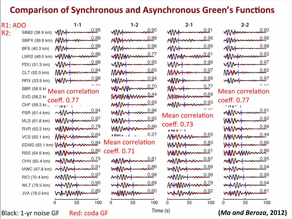
Comparison of Synchronous and Asynchronous Green’s Func+ons
Mean correlaLoncoeff. 0.77
Mean correlaLoncoeff. 0.71
Mean correlaLoncoeff. 0.73
Mean correlaLoncoeff. 0.77
R1: ADOR2:
Black: 1-‐yr noise GF Red: coda GF (Ma and Beroza, 2012)
Recommended