Berry phase Masatsugu Sei Suzuki
Department of Physics, SUNY at Binghamton (Date: May 16, 2015)
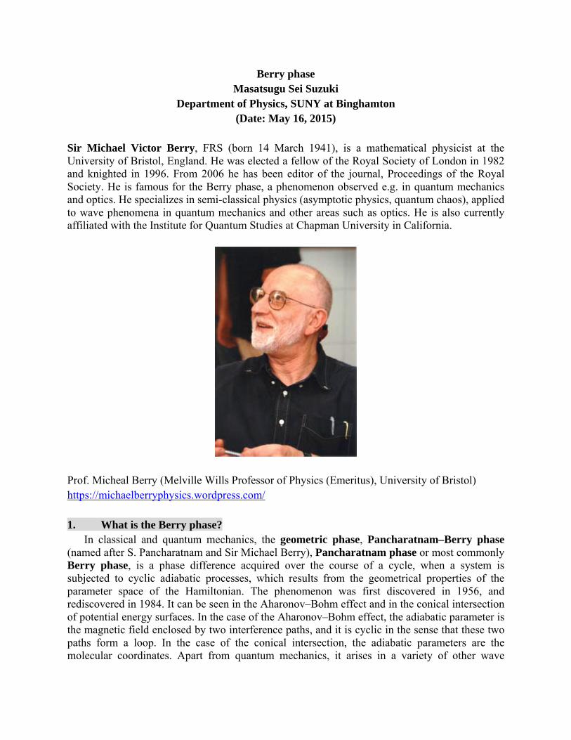
Sir Michael Victor Berry, FRS (born 14 March 1941), is a mathematical physicist at the University of Bristol, England. He was elected a fellow of the Royal Society of London in 1982 and knighted in 1996. From 2006 he has been editor of the journal, Proceedings of the Royal Society. He is famous for the Berry phase, a phenomenon observed e.g. in quantum mechanics and optics. He specializes in semi-classical physics (asymptotic physics, quantum chaos), applied to wave phenomena in quantum mechanics and other areas such as optics. He is also currently affiliated with the Institute for Quantum Studies at Chapman University in California.
Prof. Micheal Berry (Melville Wills Professor of Physics (Emeritus), University of Bristol) https://michaelberryphysics.wordpress.com/ 1. What is the Berry phase?
In classical and quantum mechanics, the geometric phase, Pancharatnam–Berry phase (named after S. Pancharatnam and Sir Michael Berry), Pancharatnam phase or most commonly Berry phase, is a phase difference acquired over the course of a cycle, when a system is subjected to cyclic adiabatic processes, which results from the geometrical properties of the parameter space of the Hamiltonian. The phenomenon was first discovered in 1956, and rediscovered in 1984. It can be seen in the Aharonov–Bohm effect and in the conical intersection of potential energy surfaces. In the case of the Aharonov–Bohm effect, the adiabatic parameter is the magnetic field enclosed by two interference paths, and it is cyclic in the sense that these two paths form a loop. In the case of the conical intersection, the adiabatic parameters are the molecular coordinates. Apart from quantum mechanics, it arises in a variety of other wave
systems, such as classical optics. As a rule of thumb, it can occur whenever there are at least two parameters characterizing a wave in the vicinity of some sort of singularity or hole in the topology; two parameters are required because either the set of nonsingular states will not be simply connected, or there will be nonzero holonomy. http://en.wikipedia.org/wiki/Geometric_phase 2. General formula for phase factor M.V. Berry, Quantum Phase Factors Accompanying Adiabatic Changes, Proc. R. London A392,
45-57 (1984).
Let the Hamiltonian H be changed by varying parameter R [R = (x, y, z)] on which it depends. Then the excursion of the system between times t = 0 and t = T can be pictured as
transport round a closed path R(t) in parameter space, with Hamiltonian ))((ˆ tH R and such that
)0()( RR T . The path is called a circuit and denoted by C. For the adiabatic approximation to
apply, T must be large.
The state vector ))(t of the system evolves according to Schrödinger equation given by
))())((ˆ))())( ttHtitt
i R
.
At any instant, the natural basis consists of the eigenstates )(Rn (assumed discrete) of )(ˆ RH
for )(tRR , that satisfy
))(())(())(())((ˆ tntEtntH n RRRR ,
with energies ))(( tEn R . The eigenvalue equation implies no relation between the phases of the
eigenstates )(Rn at different R.
Adiabatically, a system prepared in one of these states ))0((Rn will evolve with
H and so be in the state ))(( tRn at t
))(()](exp[)](exp[
))(()](exp[]'))'((exp[)(0
tntiti
tntidttEi
t
nn
n
t
n
R
RR
where )(tn is a geometric phase, and the dynamical phase factor )(tn is defined by

t
nn dttEt0
'))'((1
)( R
. )(1
)( tEt nn
Plugging the solution form into the this Schrödinger equation, we get
))(())((]))(()())(())(())(([ tntEtntitntEi
tnt
i nnn RRRRRR
or
0))(()())(( tntitn n RR .
Taking the inner product with ))(( tn R we get
0))(())(()())(())(( tntntitntn n RRRR ,
Since 1))(())(( tntn RR , we have
))(())(()( tntnitn RR
))(( tn R depends on t because there is some parameter )(tR in the Hamiltonian that changes
with time.
)())(())(( ttntn RRR R
so that
)())(())(()( ttntnitn RRR R
and thus
f
i
dtntnitn
R
R
R RRR ))(())(()(
3. Expression of )(Cn
We calculate the geometric phase )(Cn as follows.
For 1nn (normalization), we have
0
x
nnn
x
n,
0
y
nnn
y
n,
0
z
nnn
z
n.
For 0mn ( mn ) (orthogonality)
0
x
mnm
x
n,
0
y
mnm
y
n,
0
z
mnm
z
n.
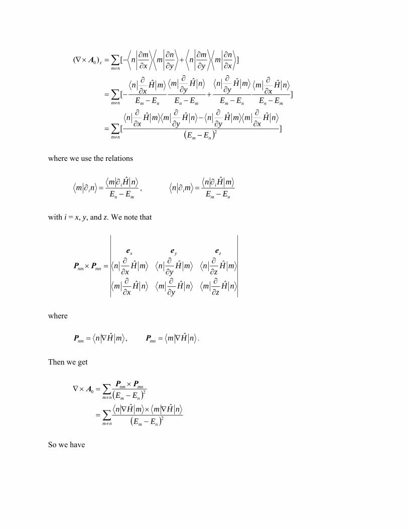
The rotation of the vector nn 0A is given by
z
yx
zyx
x
nn
yy
nn
x
z
nn
xx
nn
zy
nn
zz
nn
y
z
nn
y
nn
x
nn
zyx
nn
e
ee
eee
A
][
][][
0
nm
nm
m
z
x
nm
y
mn
y
nm
x
mn
x
nmm
y
n
y
nmm
x
n
x
nmm
y
n
y
nmm
x
n
x
n
y
n
y
n
x
n
x
n
yn
x
n
y
n
y
n
xn
y
n
x
n
x
nn
yy
nn
x
][
][
][
)( 0A
where we use the closure relation and the relations
x
mnm
x
n
, y
mnm
y
n
.
Then we obtain
nm nm
nm mnnmmnnm
nmz
EE
nHx
mmHy
nnHy
mmHx
n
EE
nHx
m
EE
mHy
n
EE
nHy
m
EE
mHx
n
x
nm
y
mn
y
nm
x
mn
]
ˆˆˆˆ
[
]
ˆˆˆˆ
[
][)(
2
0A
where we use the relations
mn
ii EE
nHmnm
ˆ
, nm
ii EE
mHnmn
ˆ
with i = x, y, and z. We note that
nHz
mnHy
mnHx
m
mHz
nmHy
nmHx
n
zyx
mnnm
ˆˆˆ
ˆˆˆ
eee
PP
where
mHnnmˆP , nHmmn
ˆP .
Then we get
nm nm
nm nm
mnnm
EE
nHmmHn
EE
2
20
ˆˆ
PPA
So we have
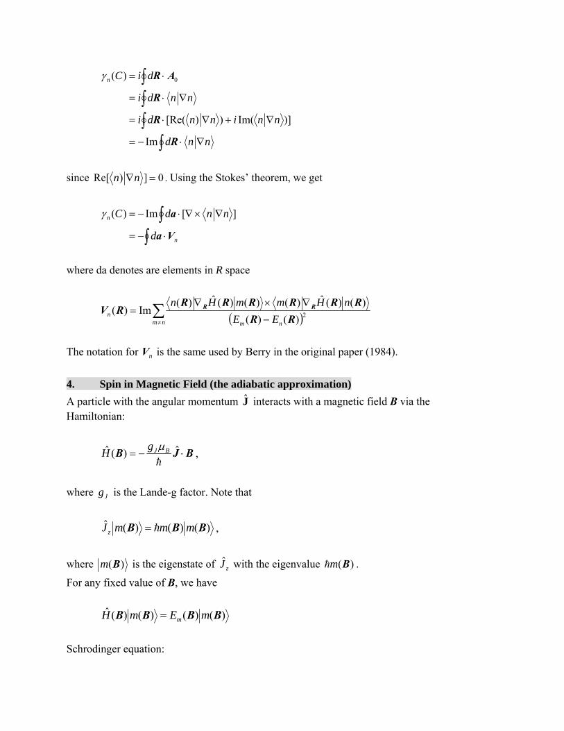
nnd
nninndi
nndi
diCn
R
R
R
AR
Im
)]Im())[Re(
)( 0
since 0])Re[ nn . Using the Stokes’ theorem, we get
n
n
d
nndC
Va
a ][Im)(
where da denotes are elements in R space
nm nm
nEE
nHmmHn2)()(
)()(ˆ)()()(ˆ)(Im)(
RR
RRRRRRRV RR
The notation for nV is the same used by Berry in the original paper (1984).
4. Spin in Magnetic Field (the adiabatic approximation)
A particle with the angular momentum J interacts with a magnetic field B via the Hamiltonian:
BJB ˆ)(ˆ
BJgH
,
where Jg is the Lande-g factor. Note that
)()()(ˆ BBB mmmJz ,
where )(Bm is the eigenstate of zJ with the eigenvalue )(Bm .
For any fixed value of B, we have
)()()()(ˆ BBBB mEmH m
Schrodinger equation:

)())(()()]([ˆ)( ttEttHtt
i m BB
with
))0(()0( tmt B
where ))0((Bm is the eigenstate of ))0((ˆ tH B .
)](exp[)](exp[))((
)](exp[]'))'((exp[))(()(0
tititm
tidttEi
tmt
mm
m
t
m
B
BB
where
t
mm dttEt0
'))'((1
)( B
Plugging the solution form into the this Schrodinger equation, we get
))(())((])(
))(())(())(())(([ tmtEt
titmtmtE
itm
ti m
mm BBBBBB
or
t
ttmtmi m
)(
))(())((
BB
Taking the inner product with ))(( tm B we get
))(())(()(
))(())(( tmtmt
ttmtmi m BBBB
,
Since 1))(())(( tmtm BB , we have
))(())(()(
tmtmit
tm BB
or
t
m dttmtmit0
'))'(())'(()( BB
Note that )(tm is real, since
0]))(())((Re[))(())(())(())(( tmtmtmtmtmtm BBBBBB
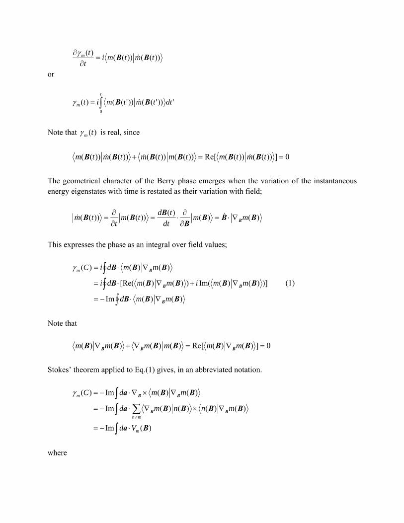
The geometrical character of the Berry phase emerges when the variation of the instantaneous energy eigenstates with time is restated as their variation with field;
)()()(
))(())(( BBBB
BBB Bmm
dt
tdtm
ttm
This expresses the phase as an integral over field values;
)()(Im
)])()(Im())()([Re(
)()()(
BBB
BBBBB
BBB
B
BB
B
mmd
mmimmdi
mmdiCm
(1)
Note that
0])()(Re[)()()()( BBBBBB BBB mmmmmm
Stokes’ theorem applied to Eq.(1) gives, in an abbreviated notation.
)(Im
)()()()(Im
)()(Im)(
Ba
BBBBa
BBa
BB
BB
m
mn
m
Vd
mnnmd
mmdC
where
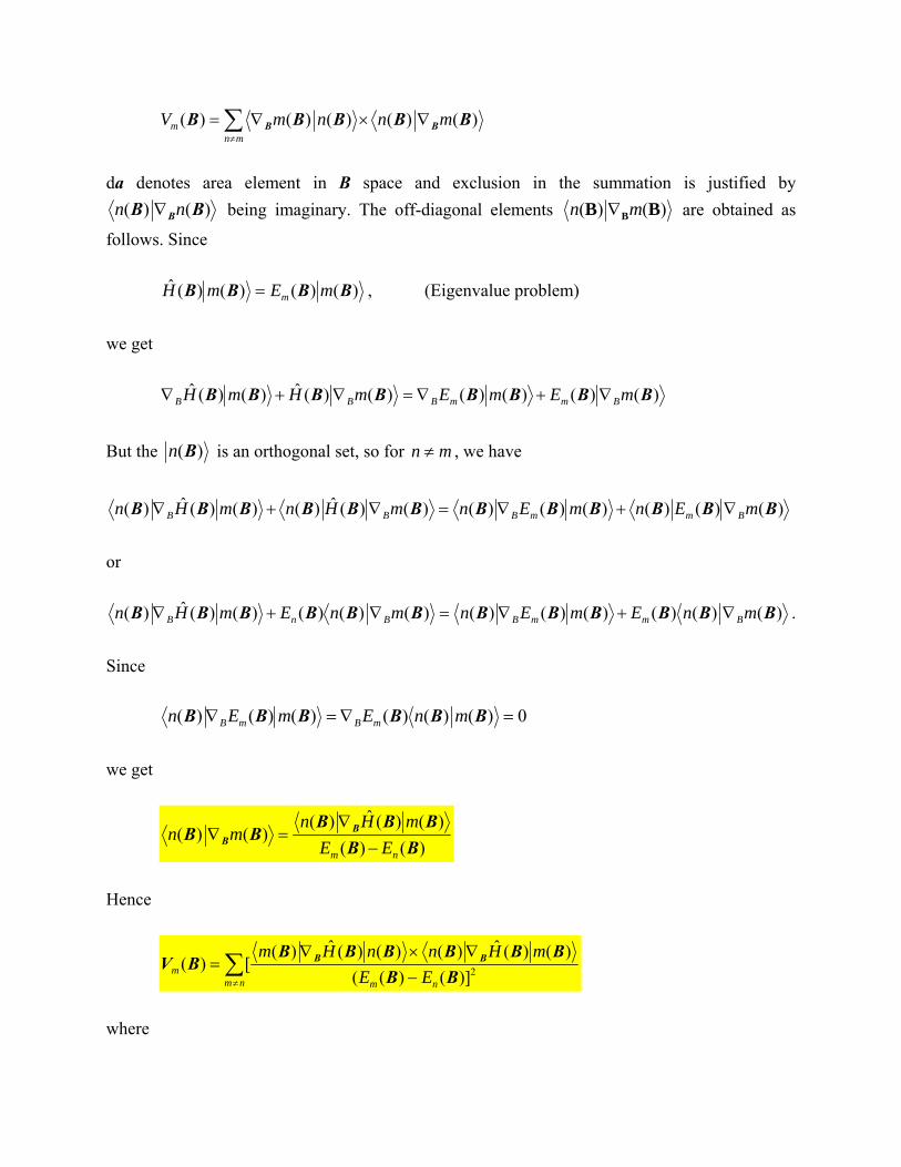
)()()()()( BBBBB BB mnnmVmn
m
da denotes area element in B space and exclusion in the summation is justified by
)()( BB Bnn being imaginary. The off-diagonal elements )()( BB Bmn are obtained as
follows. Since
)()()()(ˆ BBBB mEmH m , (Eigenvalue problem)
we get
)()()()()()(ˆ)()(ˆ BBBBBBBB mEmEmHmH BmmBBB
But the )(Bn is an orthogonal set, so for mn , we have
)()()()()()()()(ˆ)()()(ˆ)( BBBBBBBBBBBB mEnmEnmHnmHn BmmBBB
or
)()()()()()()()()()()(ˆ)( BBBBBBBBBBBB mnEmEnmnEmHn BmmBBnB .
Since
0)()()()()()( BBBBBB mnEmEn mBmB
we get
)()(
)()(ˆ)()()(
BB
BBBBB B
Bnm EE
mHnmn
Hence
nm nmm EE
mHnnHm2)]()((
)()(ˆ)()()(ˆ)([)(
BB
BBBBBBBV BB
where
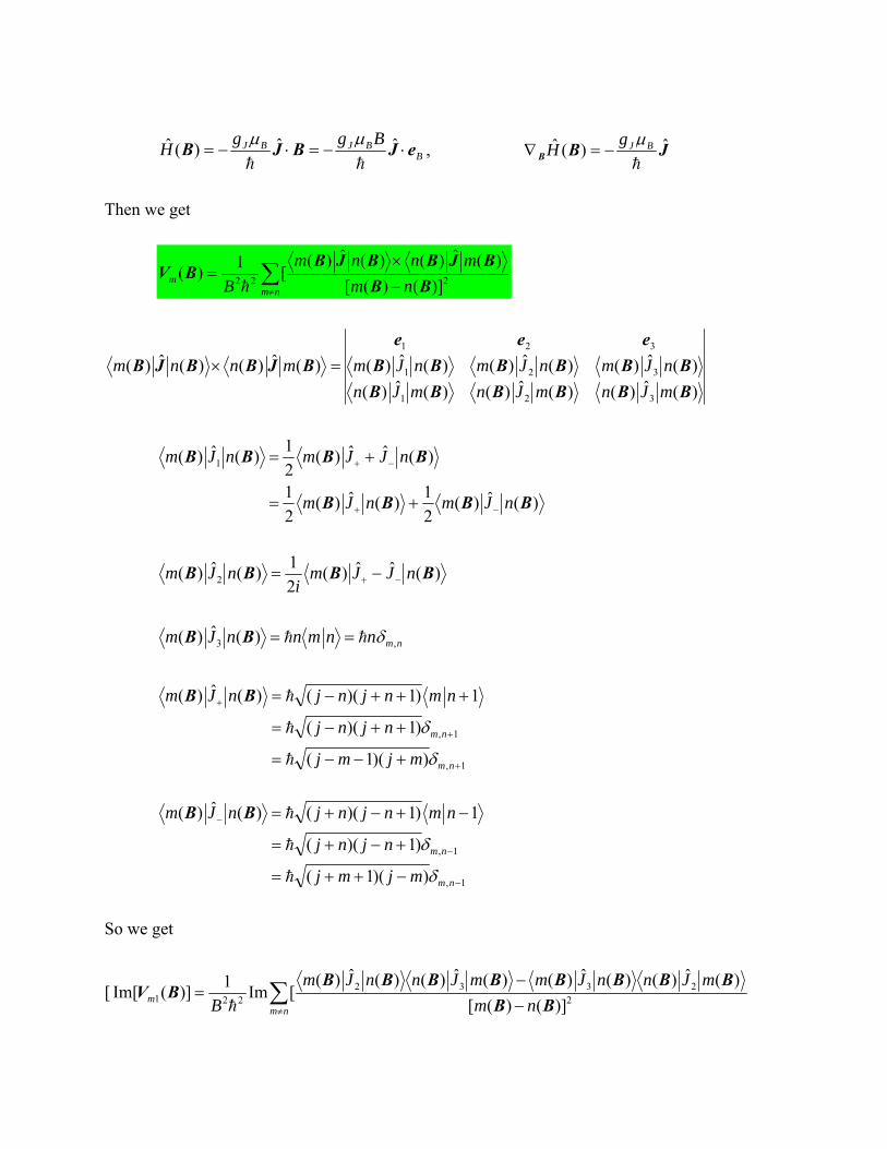
BBJBJ Bgg
H eJBJB ˆˆ)(ˆ
, JBB
ˆ)(ˆ
BJgH
Then we get
nmm nm
mnnm
B 222 )]()([
)(ˆ)()(ˆ)([
1)(
BB
BJBBJBBV
)(ˆ)()(ˆ)()(ˆ)(
)(ˆ)()(ˆ)()(ˆ)()(ˆ)()(ˆ)(
321
321
321
BBBBBB
BBBBBB
eee
BJBBJB
mJnmJnmJn
nJmnJmnJmmnnm
)(ˆ)(2
1)(ˆ)(
2
1
)(ˆˆ)(2
1)(ˆ)( 1
BBBB
BBBB
nJmnJm
nJJmnJm
)(ˆˆ)(2
1)(ˆ)( 2 BBBB nJJm
inJm
nmnnmnnJm ,3 )(ˆ)( BB
1,
1,
))(1(
)1)((
1)1)(()(ˆ)(
nm
nm
mjmj
njnj
nmnjnjnJm
BB
1,
1,
))(1(
)1)((
1)1)(()(ˆ)(
nm
nm
mjmj
njnj
nmnjnjnJm
BB
So we get
[
nmm nm
mJnnJmmJnnJm
B 22332
221 )]()([
)(ˆ)()(ˆ)()(ˆ)()(ˆ)([Im
1)](Im[
BB
BBBBBBBBBV
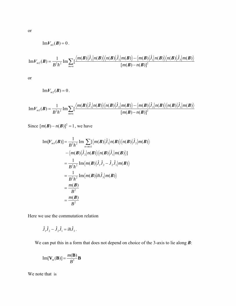
or
0)(Im 1 BVm .
nmm nm
mJnnJmmJnnJm
B 23113
222 )]()([
)(ˆ)()(ˆ)()(ˆ)()(ˆ)([Im
1)(Im
BB
BBBBBBBBBV
or
0)(Im 2 BVm .
nmm nm
mJnnJmmJnnJm
B 21221
223 )]()([
)(ˆ)()(ˆ)()(ˆ)()(ˆ)([Im
1)(Im
BB
BBBBBBBBBV
Since 1)]()([ 2 BB nm , we have
2
2
322
122122
12
121223
)(
)(
)(ˆ)(Im1
)(ˆˆˆˆ)(Im1
])(ˆ)()(ˆ)(
)(ˆ)()(ˆ)([Im1
)](Im[
B
mB
m
mJimB
mJJJJmB
mJnnJm
mJnnJmB mn
m
B
B
BB
BB
BBBB
BBBBBV
Here we use the commutation relation
31221ˆˆˆˆˆ JiJJJJ .
We can put this in a form that does not depend on choice of the 3-axis to lie along B:
BB
BV3
)()](Im[
B
mm
We note that is

)(41
BB B
where
3
1
BB
BB
This singularity is spherically symmetric. The Berry phase is given by
)()0()()(
)(Im)(3
CmmCB
mdVdC mm BB
BaBa
where )(C is the solid angle subtended by C as seen from the origin in field space .
)()1
(1
22
3Cd
BdB
Bd BB eeBa
((Note)) Vector analysis: Gauss’ law
41
)]1
([)]1
[ 3
2 B
Bd
Bd
Bd
Bd aaBB BBBB
where
3
1
BB
BB .
We have
)(41
)1
( 2 BBB BB B
where )(B is the Dirac delta function.
)cos1(2sin2
00
dd

5. Example: spin ½ under the magnetic field which undergoes a precession
adiabatically
The magnetic field is given by
cos
sinsin
cossin
0BB
with
t .
Spin magnetic moment: σSμ ˆˆ2ˆ B
Bs
.
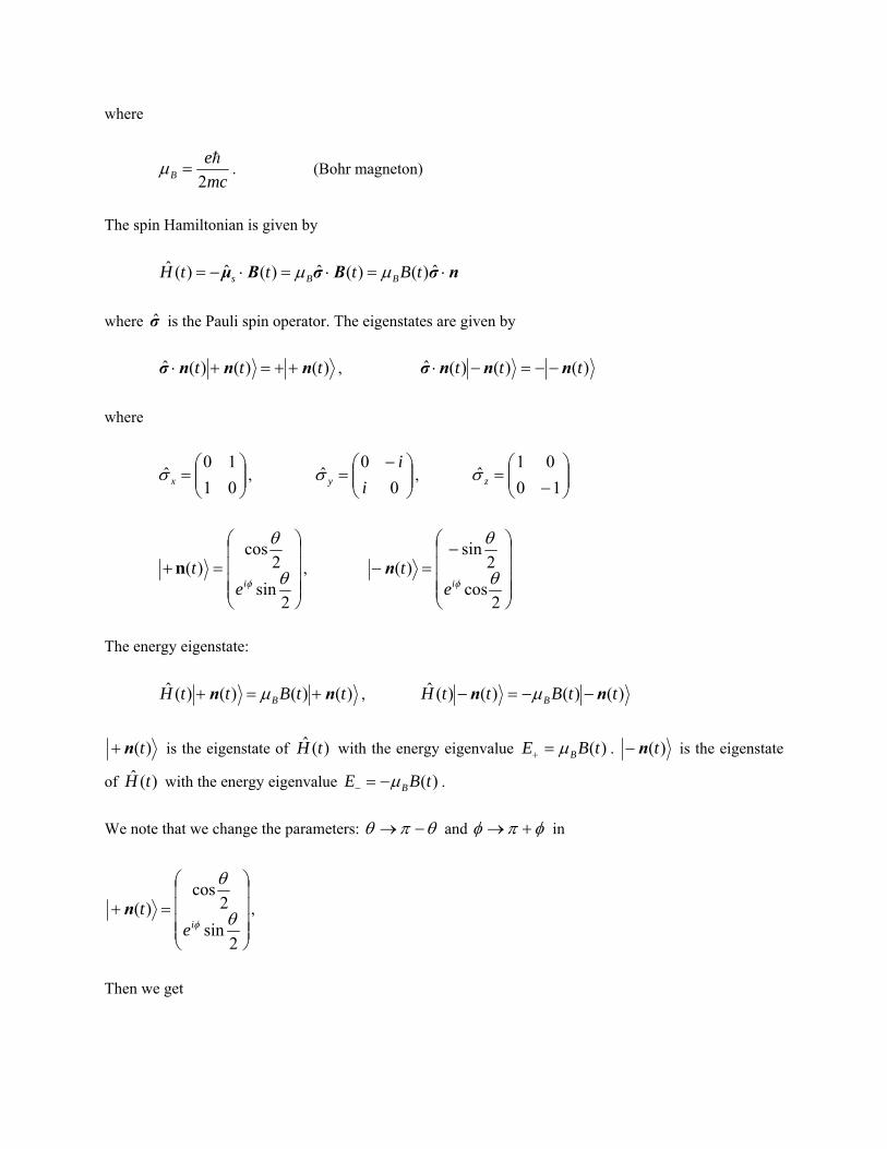
where
mc
eB 2
. (Bohr magneton)
The spin Hamiltonian is given by
nσBσBμ ˆ)()(ˆ)(ˆ)(ˆ tBtttH BBs
where σ is the Pauli spin operator. The eigenstates are given by
)()()(ˆ ttt nnnσ , )()()(ˆ ttt nnnσ
where
01
10ˆ x ,
0
0ˆ
i
iy ,
10
01ˆ z
2sin
2cos
)(
ietn ,
2cos
2sin
)(
ietn
The energy eigenstate:
)()()()(ˆ ttBttH B nn , )()()()(ˆ ttBttH B nn
)(tn is the eigenstate of )(ˆ tH with the energy eigenvalue )(tBE B . )(tn is the eigenstate
of )(ˆ tH with the energy eigenvalue )(tBE B .
We note that we change the parameters: and in
2sin
2cos
)(
ietn ,
Then we get
2cos
2sin
)(
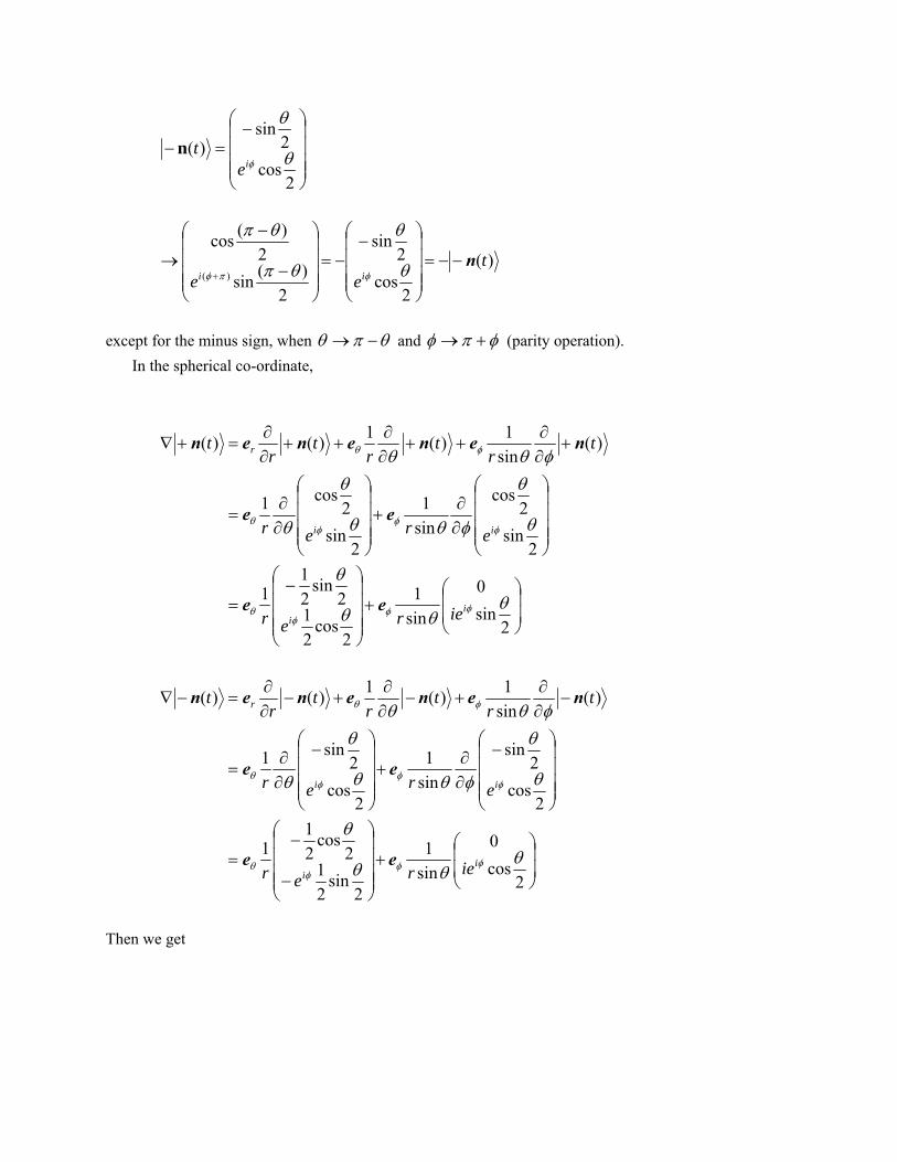
ietn
)(
2cos
2sin
2
)(sin
2
)(cos
)(t
ee iin
except for the minus sign, when and (parity operation).
In the spherical co-ordinate,
2sin
0
sin
1
2cos
2
12
sin2
11
2sin
2cos
sin
1
2sin
2cos1
)(sin
1)(
1)()(
ii
ii
r
ierer
erer
tr
tr
tr
t
ee
ee
nenenen
2cos
0
sin
1
2sin
2
12
cos2
11
2cos
2sin
sin
1
2cos
2sin1
)(sin
1)(
1)()(
ii
ii
r
ierer
erer
tr
tr
tr
t
ee
ee
nenenen
Then we get
sin2
sin
2sin
0
2sin
2cos
sin
1
2cos
2
12
sin2
1
2sin
2cos
1)()(
2
r
i
ieer
ee
rtt
ii
i
i
e
e
enn
where
2sin
2cos)(
ietn .
sin2
cos
2cos
0
2cos
2sin
sin
1
2sin
2
12
cos2
1
2cos
2sin
1)()(
2
r
i
ieer
ee
rtt
ii
i
i
e
e
enn
where
2cos
2sin)(
ietn .
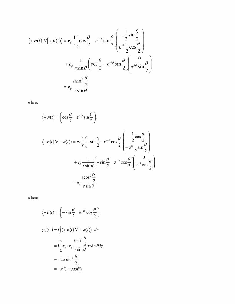
)cos1(2
sin2
sinsin
2sin
)()()(
2
2
0
2
drr
ii
dttiC
ee
rnn
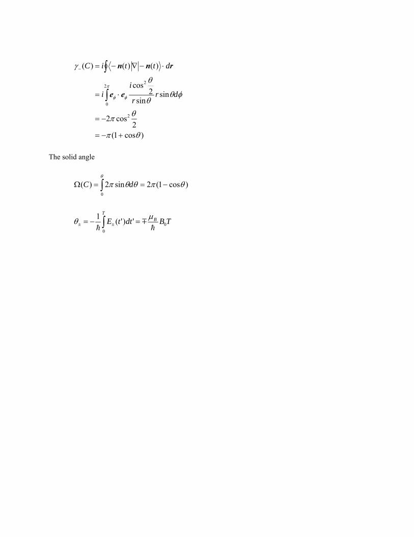
)cos1(2
cos2
sinsin
2cos
)()()(
2
2
0
2
drr
ii
dttiC
ee
rnn
The solid angle
)cos1(2sin2)(0
dC
TBdttE BT
0
0
')'(1


The final state after one rotation where 0)( BTB is then given by
)0()exp(]cos1(exp[
)()](exp[)](exp[)(
0 nTBii
TnTiTiT
B
nn
We see that the dynamical phase factor depends on the period T of the rotation, but the geometrical phase depends only on the special geometry of the problem. In this case it depends on the opening angle q of the cone that the magnetic field traces out.
______________________________________________________________________________ REFERENCES
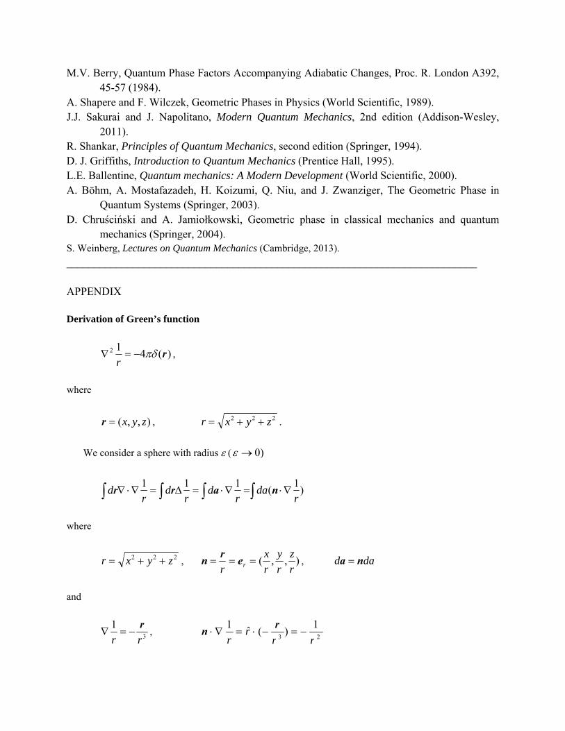
M.V. Berry, Quantum Phase Factors Accompanying Adiabatic Changes, Proc. R. London A392, 45-57 (1984).
A. Shapere and F. Wilczek, Geometric Phases in Physics (World Scientific, 1989). J.J. Sakurai and J. Napolitano, Modern Quantum Mechanics, 2nd edition (Addison-Wesley,
2011). R. Shankar, Principles of Quantum Mechanics, second edition (Springer, 1994). D. J. Griffiths, Introduction to Quantum Mechanics (Prentice Hall, 1995). L.E. Ballentine, Quantum mechanics: A Modern Development (World Scientific, 2000). A. Böhm, A. Mostafazadeh, H. Koizumi, Q. Niu, and J. Zwanziger, The Geometric Phase in
Quantum Systems (Springer, 2003). D. Chruściński and A. Jamiołkowski, Geometric phase in classical mechanics and quantum
mechanics (Springer, 2004). S. Weinberg, Lectures on Quantum Mechanics (Cambridge, 2013).
__________________________________________________________________________ APPENDIX Derivation of Green’s function
)(412 rr
,
where
),,( zyxr , 222 zyxr .
We consider a sphere with radius ( )0
)1
(111
rda
rd
rd
rd narr
where
222 zyxr , ),,(r
z
r
y
r
x
r r er
n , dad na
and
3
1
rr
r ,
23
1)(ˆ
1
rrr
r
rn

We now
surface of
connected
Since
Using the
V
or
A
0)1
( r
e
consider the
f sphere A' (v
d to an approp
0)1
( r
ov
Gauss's law,
1
'
V r
dr
)1
(A rda n
except at the
volume integ
volume V', rad
priate cylinde
ver the whole
we get
(
'
2
A
VV
da
rd
n
r
'
'('A
da n
origin.
gral over the
dius )0r.
volume V - V
'(')1
1
'
A
dar
r
n
'
(')1
A
dar
n
e whole volum
. We note tha
V' we have
0)1
r
)1
rn
me (V - V') b
at the outer su
between the
urface and th
surface A an
he inner surfac
nd the
ce are
where r' nn and dr is over the volume integral. Then we have
)(441
4)1
()1
(2
22
rrn
dr
dar
daA
Using the Gauss's law, we have
VVA
dr
dr
da )(4)1
()1
( rrrn
or
)(41
rr
.
or
)()4
1( r
r
.
((Mathematica))
Clear"Gobal`";
Needs"VectorAnalysis`"SetCoordinatesCartesianx, y, zCartesianx, y, z
r1 x, y, z; r r1.r1
x2 y2 z2
Grad1
r Simplify
x
x2 y2 z232,
y
x2 y2 z232,
z
x2 y2 z232
Laplacian1
r Simplify
0
Recommended