[email protected] • ENGR-25_Plot_Model-4.ppt1
Bruce Mayer, PE Engineering/Math/Physics 25: Computational Methods
Bruce Mayer, PERegistered Electrical & Mechanical Engineer
Engr/Math/Physics 25
Chp6 MATLAB
Regression
[email protected] • ENGR-25_Plot_Model-4.ppt2
Bruce Mayer, PE Engineering/Math/Physics 25: Computational Methods
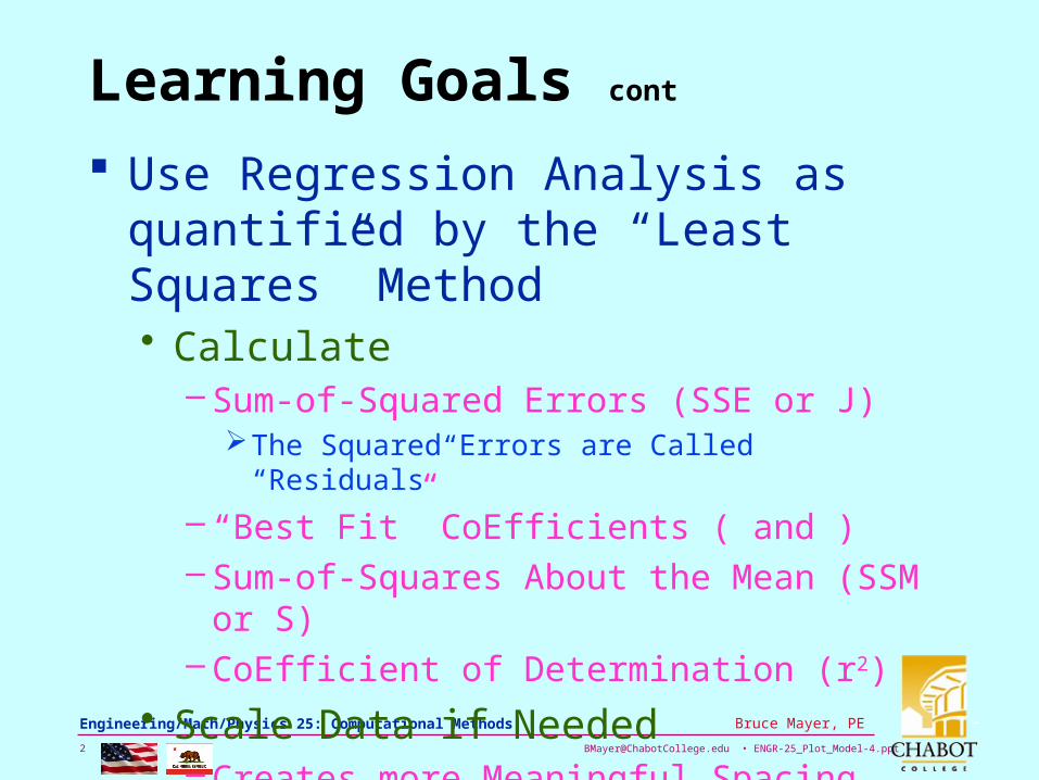
Learning Goals cont
Use Regression Analysis as quantified by the “Least Squares” Method• Calculate–Sum-of-Squared Errors (SSE or J)The Squared Errors are Called “Residuals”
– “Best Fit” CoEfficients ( and )–Sum-of-Squares About the Mean (SSM or S)–CoEfficient of Determination (r2)
• Scale Data if Needed–Creates more Meaningful Spacing
[email protected] • ENGR-25_Plot_Model-4.ppt3
Bruce Mayer, PE Engineering/Math/Physics 25: Computational Methods
Learning Goals cont
Build Math Models for Physical Data using “nth” Degree Polynomials
Use MATLAB’s “Basic Fitting” Utility to find Math models for Plotted Data
[email protected] • ENGR-25_Plot_Model-4.ppt4
Bruce Mayer, PE Engineering/Math/Physics 25: Computational Methods
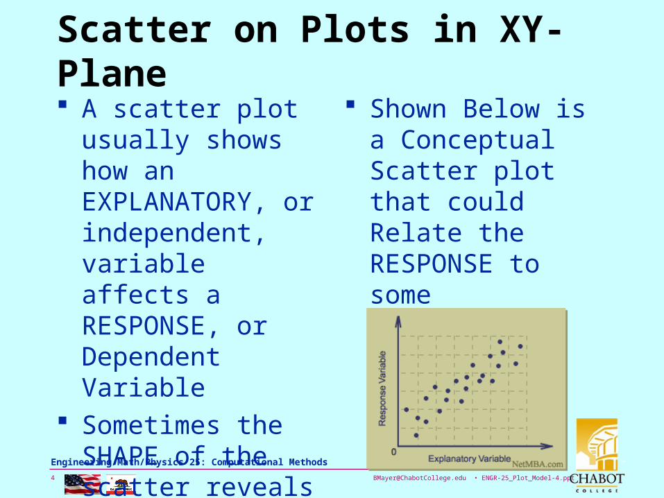
Scatter on Plots in XY-Plane A scatter plot usually
shows how an EXPLANATORY, or independent, variable affects a RESPONSE, or Dependent Variable
Sometimes the SHAPE of the scatter reveals a relationship
Shown Below is a Conceptual Scatter plot that could Relate the RESPONSE to some EXCITITATION
[email protected] • ENGR-25_Plot_Model-4.ppt5
Bruce Mayer, PE Engineering/Math/Physics 25: Computational Methods
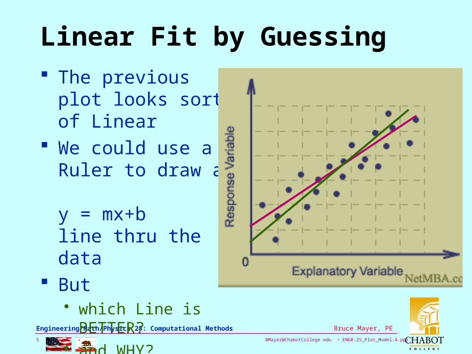
Linear Fit by Guessing The previous plot
looks sort of Linear We could use a
Ruler to draw a y = mx+b line thru the data
But • which Line is
BETTER?• and WHY?
[email protected] • ENGR-25_Plot_Model-4.ppt6
Bruce Mayer, PE Engineering/Math/Physics 25: Computational Methods
Least Squares Curve Fitting
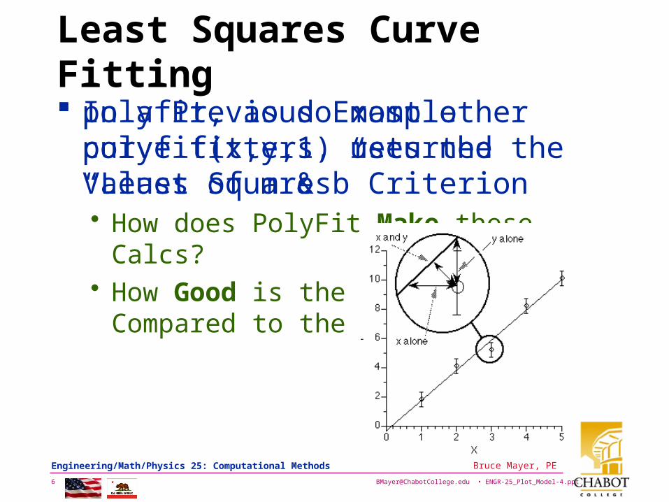
In a Previous Example polyfit(x,y,1) returned the Values of m & b• How does PolyFit Make these Calcs?• How Good is the fitted Line Compared to
the Data?
polyfit, as do most other curve fitters, uses the “Least Squares” Criterion
[email protected] • ENGR-25_Plot_Model-4.ppt7
Bruce Mayer, PE Engineering/Math/Physics 25: Computational Methods
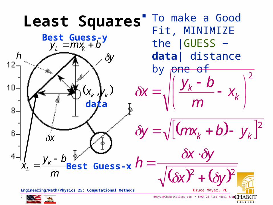
Least Squares
y
kk yx ,
hbmxy kL
m
byx kL
x
To make a Good Fit, MINIMIZE the |GUESS − data| distance by one of
22
2
2
yx
yxh
ybmxy
xm
byx
kk
kk
data
Best Guess-y
Best Guess-x
[email protected] • ENGR-25_Plot_Model-4.ppt8
Bruce Mayer, PE Engineering/Math/Physics 25: Computational Methods
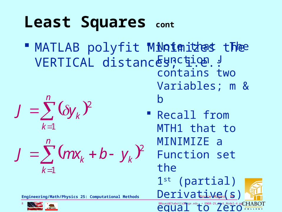
Least Squares cont
MATLAB polyfit Minimizes the VERTICAL distances; i.e.:
n
kkk
n
kk
ybmxJ
yJ
1
2
1
2
Note that The Function J contains two Variables; m & b
Recall from MTH1 that to MINIMIZE a Function set the 1st (partial) Derivative(s) equal to Zero
[email protected] • ENGR-25_Plot_Model-4.ppt9
Bruce Mayer, PE Engineering/Math/Physics 25: Computational Methods
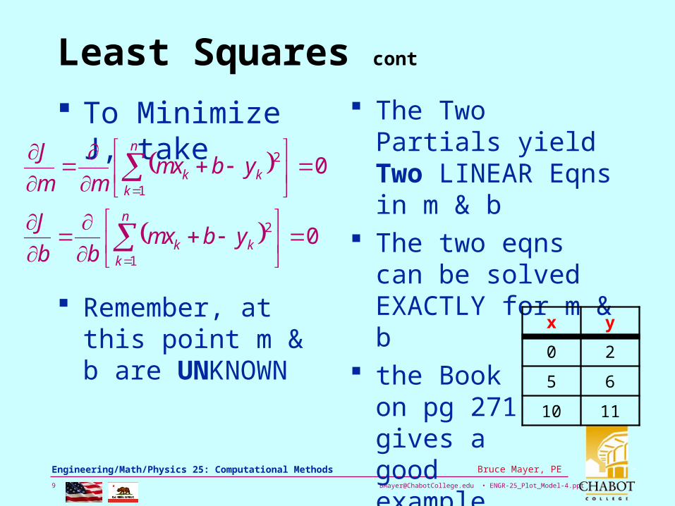
Least Squares cont
To Minimize J, take
0
0
1
2
1
2
n
kkk
n
kkk
ybmxbb
J
ybmxmm
J
The Two Partials yield Two LINEAR Eqns in m & b
The two eqns can be solved EXACTLY for m & b
the Book on pg 271 gives a good example
Remember, at this point m & b are UNKNOWN
x y
0 2
5 6
10 11
[email protected] • ENGR-25_Plot_Model-4.ppt10
Bruce Mayer, PE Engineering/Math/Physics 25: Computational Methods
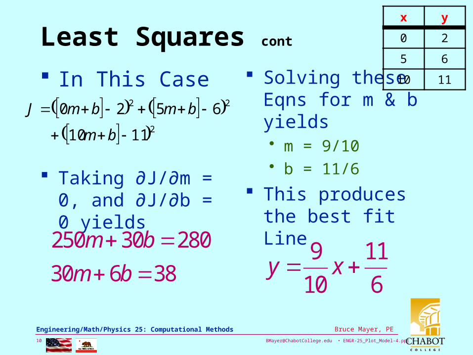
Least Squares cont
In This Case 2
22
1110
6520
bm
bmbmJ
Solving theseEqns for m & b yields• m = 9/10• b = 11/6
This produces the best fit Line
Taking ∂J/∂m = 0, and ∂J/∂b = 0 yields
x y
0 2
5 6
10 11
38630
28030250
bm
bm
6
11
10
9 xy
[email protected] • ENGR-25_Plot_Model-4.ppt11
Bruce Mayer, PE Engineering/Math/Physics 25: Computational Methods
Goodness of Fit
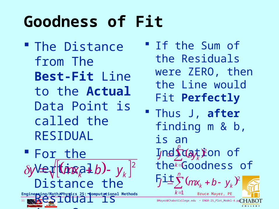
The Distance from The Best-Fit Line to the Actual Data Point is called the RESIDUAL
For the Vertical Distance the Residual is just δy
If the Sum of the Residuals were ZERO, then the Line would Fit Perfectly
Thus J, after finding m & b, is an Indication of the Goodness of Fit
2kk ybmxy
n
kkk
n
kk
ybmxJ
yJ
1
2
1
2
[email protected] • ENGR-25_Plot_Model-4.ppt12
Bruce Mayer, PE Engineering/Math/Physics 25: Computational Methods
Goodness of Fit cont
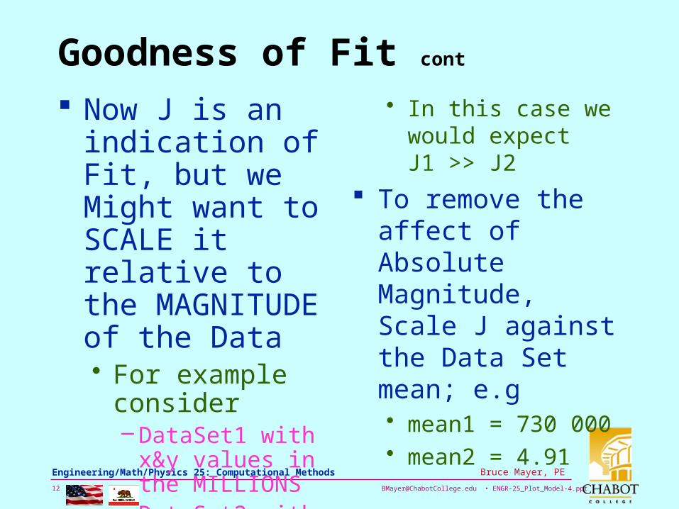
Now J is an indication of Fit, but we Might want to SCALE it relative to the MAGNITUDE of the Data• For example
consider–DataSet1 with x&y
values in the MILLIONS–DataSet2 with x&y
values in the single digits
• In this case we would expect J1 >> J2
To remove the affect of Absolute Magnitude, Scale J against the Data Set mean; e.g• mean1 = 730 000• mean2 = 4.91
[email protected] • ENGR-25_Plot_Model-4.ppt13
Bruce Mayer, PE Engineering/Math/Physics 25: Computational Methods
Goodness of Fit cont
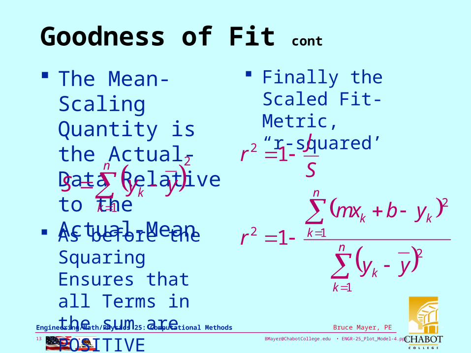
The Mean-Scaling Quantity is the Actual-Data Relative to the Actual-Mean
Finally the Scaled Fit-Metric, “r-squared’
2
1
n
kk yyS
n
kk
n
kkk
yy
ybmxr
S
Jr
1
2
1
2
2
2
1
1
As before the Squaring Ensures that all Terms in the sum are POSITIVE
[email protected] • ENGR-25_Plot_Model-4.ppt14
Bruce Mayer, PE Engineering/Math/Physics 25: Computational Methods
r2 = Coeff of Determination
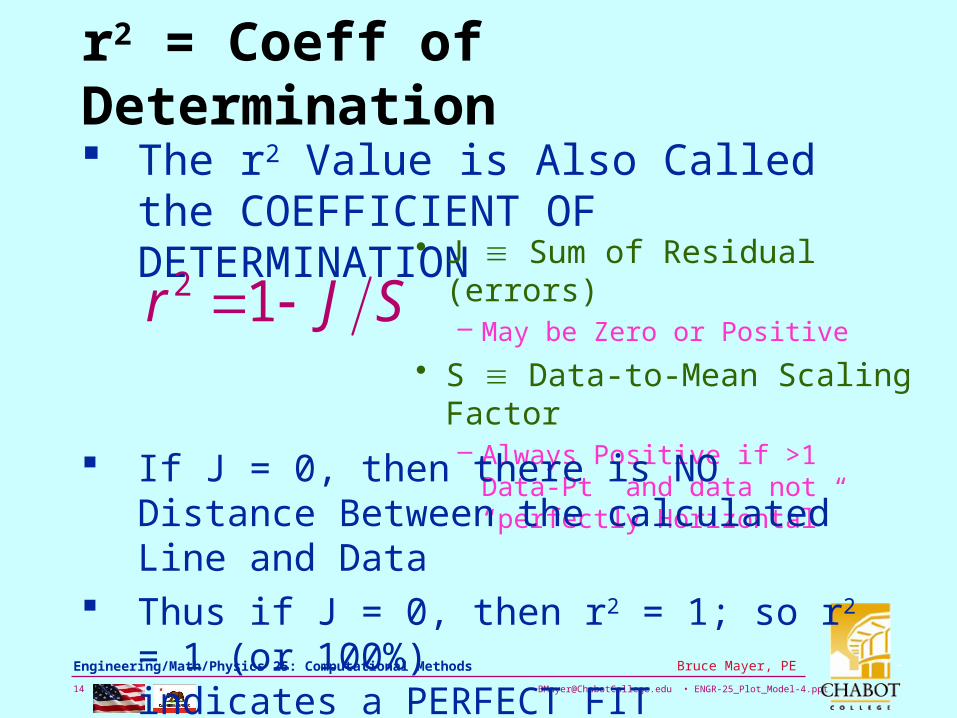
The r2 Value is Also Called the COEFFICIENT OF DETERMINATION
SJr 12• J Sum of Residual (errors)
– May be Zero or Positive
• S Data-to-Mean Scaling Factor– Always Positive if >1 Data-Pt and
data not “perfectly Horizontal”
If J = 0, then there is NO Distance Between the calculated Line and Data
Thus if J = 0, then r2 = 1; so r2 = 1 (or 100%)indicates a PERFECT FIT
[email protected] • ENGR-25_Plot_Model-4.ppt15
Bruce Mayer, PE Engineering/Math/Physics 25: Computational Methods
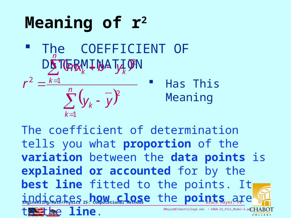
Meaning of r2
The COEFFICIENT OF DETERMINATION
n
kk
n
kkk
yy
ybmxr
1
2
1
2
2 Has This Meaning
The coefficient of determination tells you what proportion of the variation between the data points is explained or accounted for by the best line fitted to the points. It indicates how close the points are to the line.
[email protected] • ENGR-25_Plot_Model-4.ppt16
Bruce Mayer, PE Engineering/Math/Physics 25: Computational Methods
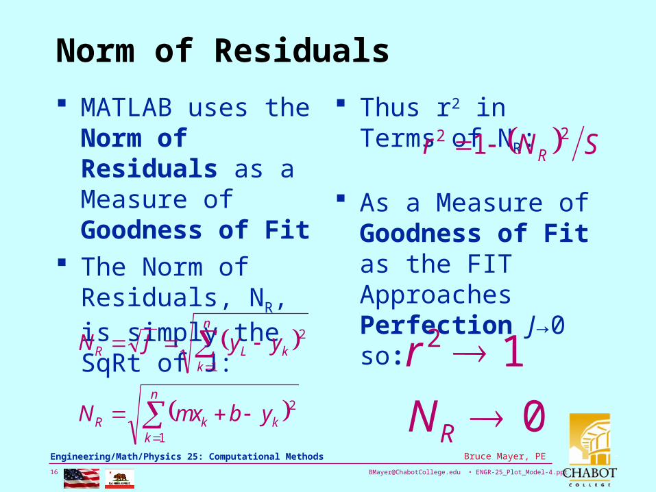
Norm of Residuals
MATLAB uses the Norm of Residuals as a Measure of Goodness of Fit
The Norm of Residuals, NR, is simply the SqRt of J:
n
kkkR
n
kkLR
ybmxN
yyJN
1
2
1
2
Thus r2 in Terms of NR:
As a Measure of Goodness of Fit as the FIT Approaches Perfection J→0 so:
0
12
RN
r
SNr R22 1
[email protected] • ENGR-25_Plot_Model-4.ppt17
Bruce Mayer, PE Engineering/Math/Physics 25: Computational Methods
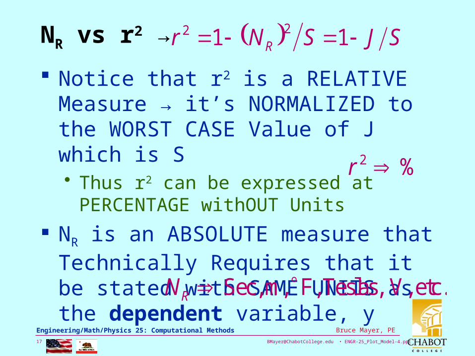
NR vs r2 → SJSNr R 11 22
Notice that r2 is a RELATIVE Measure → it’s NORMALIZED to the WORST CASE Value of J which is S• Thus r2 can be expressed at
PERCENTAGE withOUT Units
NR is an ABSOLUTE measure that Technically Requires that it be stated with SAME UNITS as the dependent variable, y
%2 r
etc. V, Teslas, F, m, Sec, RN
[email protected] • ENGR-25_Plot_Model-4.ppt18
Bruce Mayer, PE Engineering/Math/Physics 25: Computational Methods
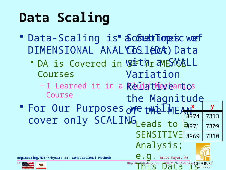
Data Scaling
Data-Scaling is a SubTopic of DIMENSIONAL ANALYIS (DA)• DA is Covered in 3rd Yr ME/CE Courses– I Learned it in a Fluid Mechanics Course
For Our Purposes we will cover only SCALING
Sometimes we Collect Data with a SMALL Variation Relative to the Magnitude of the MEAN• Leads to a
SENSITIVE Analysis; e.g. This Data is Noisy During Analysis
x y
8974 7313
8971 7309
8969 7310
[email protected] • ENGR-25_Plot_Model-4.ppt19
Bruce Mayer, PE Engineering/Math/Physics 25: Computational Methods
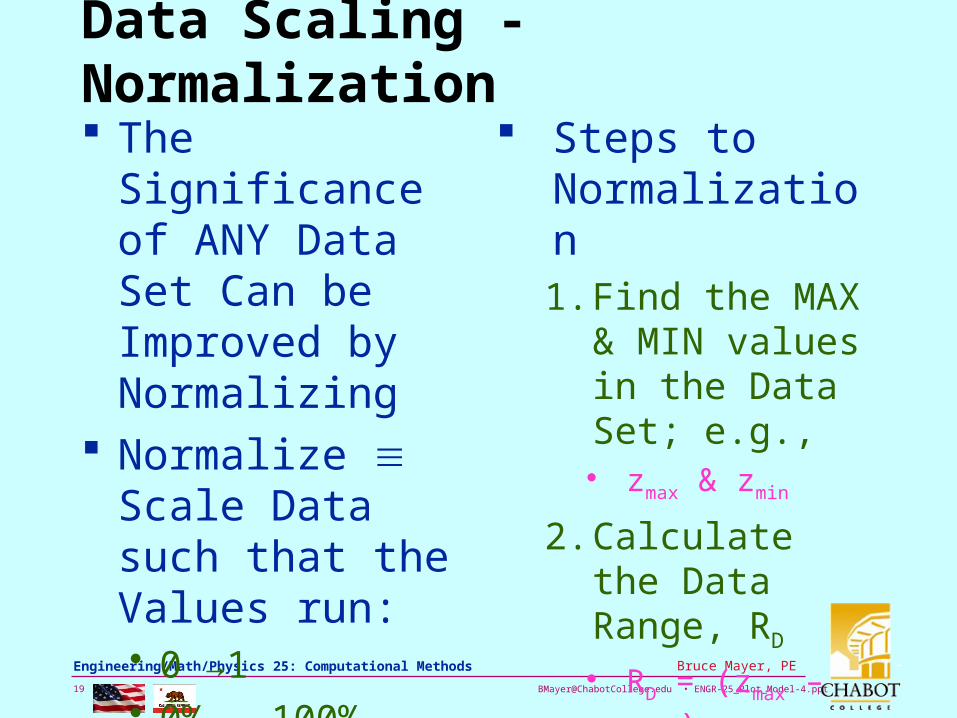
Data Scaling - Normalization
The Significance of ANY Data Set Can be Improved by Normalizing
Normalize Scale Data such that the Values run:• 0 →1• 0% → 100%
Steps to Normalization1. Find the MAX &
MIN values in the Data Set; e.g.,• zmax & zmin
2. Calculate the Data Range, RD
• RD = (zmax – zmin)
3. Calc the Individual Data Differences Relative to the MIN• Δzk = zk - zmin
[email protected] • ENGR-25_Plot_Model-4.ppt20
Bruce Mayer, PE Engineering/Math/Physics 25: Computational Methods
Data Scaling – Normailzation cont
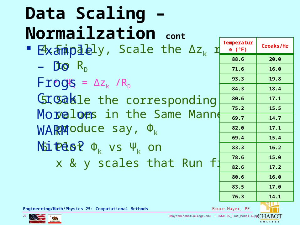
4. Finally, Scale the Δzk relative to RD
• Ψk = Δzk /RD
5. Scale the corresponding “y” values in the Same Manner to produce say, Φk
6. Plot Φk vs Ψk on x & y scales that Run from 0→1
Example– Do Frogs Croak More on WARM Nites?
Temperature (ºF)
Croaks/Hr
88.6 20.0
71.6 16.0
93.3 19.8
84.3 18.4
80.6 17.1
75.2 15.5
69.7 14.7
82.0 17.1
69.4 15.4
83.3 16.2
78.6 15.0
82.6 17.2
80.6 16.0
83.5 17.0
76.3 14.1
[email protected] • ENGR-25_Plot_Model-4.ppt21
Bruce Mayer, PE Engineering/Math/Physics 25: Computational Methods
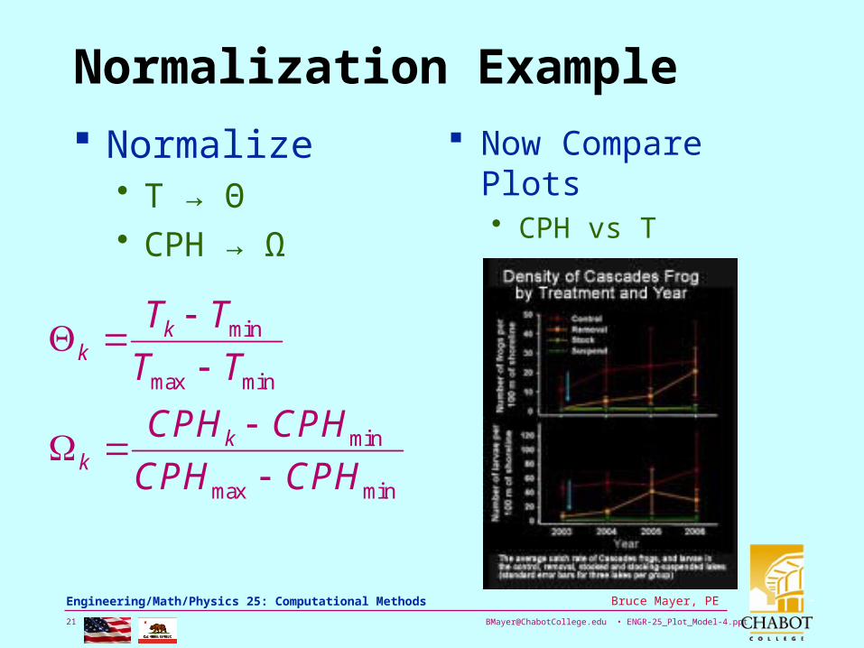
Normalization Example
Normalize• T → Θ• CPH → Ω
minmax
min
minmax
min
CPHCPH
CPHCPH
TT
TT
kk
kk
Now Compare Plots• CPH vs T• Ω vs Θ
[email protected] • ENGR-25_Plot_Model-4.ppt22
Bruce Mayer, PE Engineering/Math/Physics 25: Computational Methods
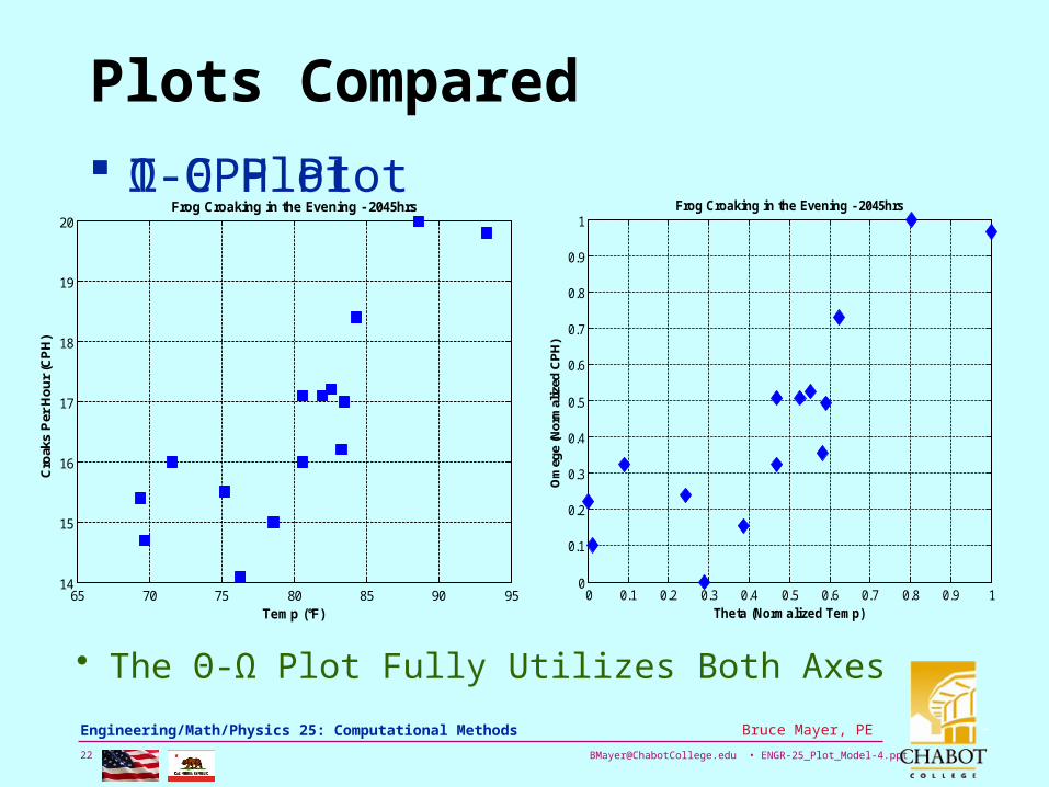
Plots Compared
T-CPH Plot Ω-Θ Plot
65 70 75 80 85 90 9514
15
16
17
18
19
20Frog Croaking in the Evening - 2045hrs
Temp (°F)
Cro
aks
Per
Ho
ur
(CP
H)
0 0.1 0.2 0.3 0.4 0.5 0.6 0.7 0.8 0.9 10
0.1
0.2
0.3
0.4
0.5
0.6
0.7
0.8
0.9
1Frog Croaking in the Evening - 2045hrs
Theta (Normalized Temp)
Om
ege
(Nor
mal
ized
CP
H)
• The Θ-Ω Plot Fully Utilizes Both Axes
[email protected] • ENGR-25_Plot_Model-4.ppt23
Bruce Mayer, PE Engineering/Math/Physics 25: Computational Methods
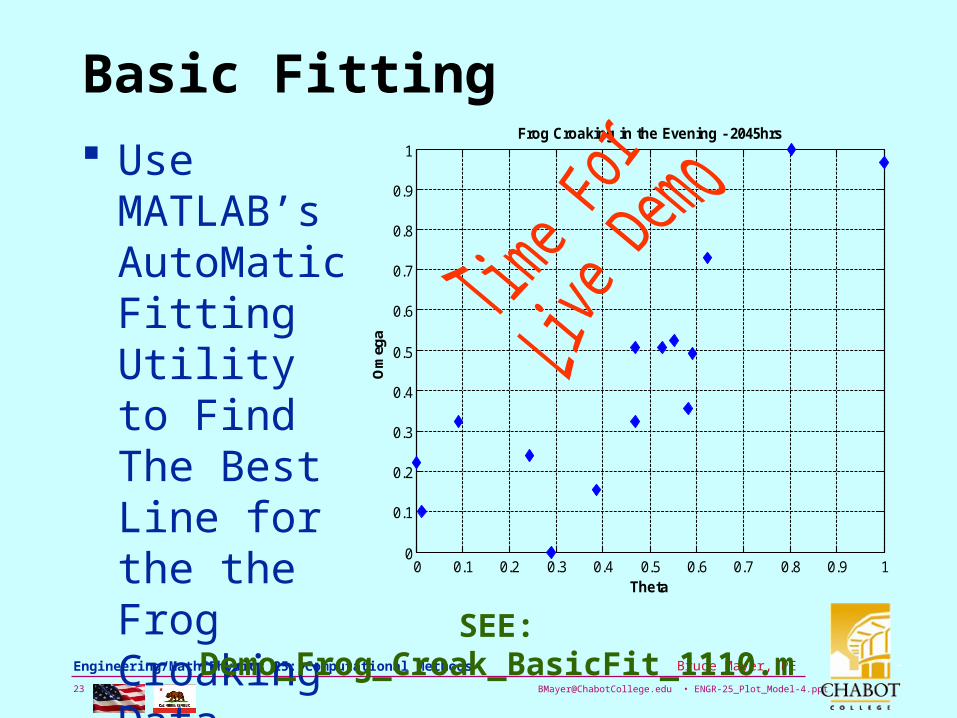
Basic Fitting
Use MATLAB’s AutoMatic Fitting Utility to Find The Best Line for the the Frog Croaking Data 0 0.1 0.2 0.3 0.4 0.5 0.6 0.7 0.8 0.9 1
0
0.1
0.2
0.3
0.4
0.5
0.6
0.7
0.8
0.9
1
Theta
Om
ega
Frog Croaking in the Evening - 2045hrs
SEE: Demo_Frog_Croak_BasicFit_1110.m

[email protected] • ENGR-25_Plot_Model-4.ppt24
Bruce Mayer, PE Engineering/Math/Physics 25: Computational Methods
All Done for Today
CroakingFrog
[email protected] • ENGR-25_Plot_Model-4.ppt25
Bruce Mayer, PE Engineering/Math/Physics 25: Computational Methods
Bruce Mayer, PELicensed Electrical & Mechanical Engineer
Engr/Math/Physics 25
Appendix 6972 23 xxxxf
[email protected] • ENGR-25_Plot_Model-4.ppt26
Bruce Mayer, PE Engineering/Math/Physics 25: Computational Methods
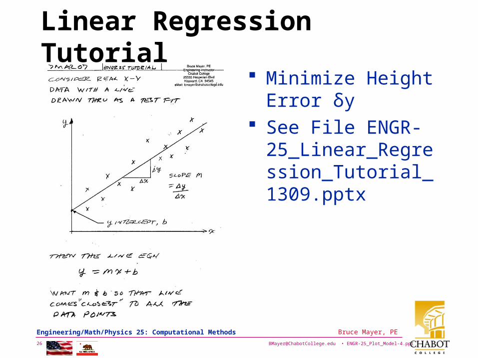
Linear Regression Tutorial Minimize Height
Error δy See File ENGR-
25_Linear_Regression_Tutorial_1309.pptx
[email protected] • ENGR-25_Plot_Model-4.ppt27
Bruce Mayer, PE Engineering/Math/Physics 25: Computational Methods
[email protected] • ENGR-25_Plot_Model-4.ppt28
Bruce Mayer, PE Engineering/Math/Physics 25: Computational Methods
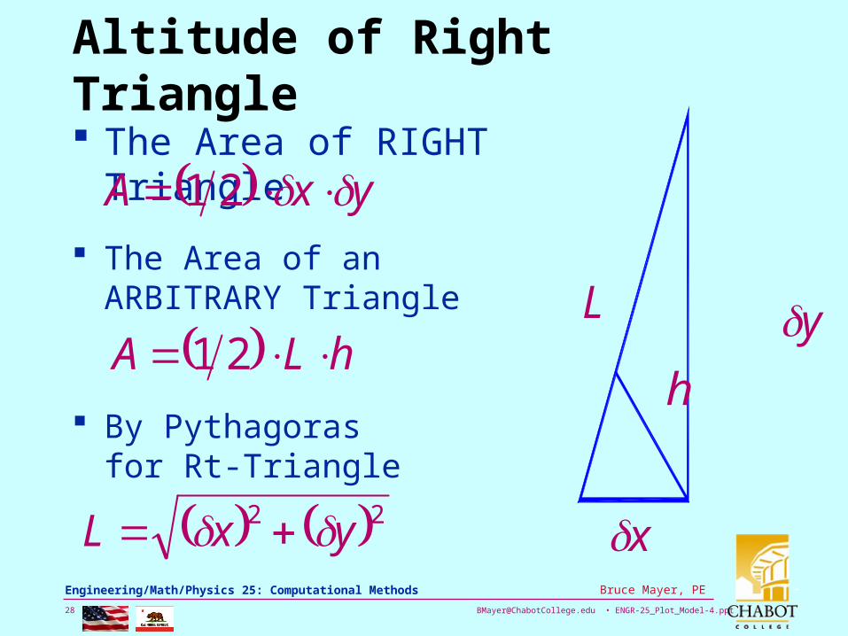
Altitude of Right Triangle
The Area of RIGHT Triangle
y
x
L
h
yxA 21 The Area of an ARBITRARY
Triangle
hLA 21
By Pythagoras for Rt-Triangle
22 yxL
[email protected] • ENGR-25_Plot_Model-4.ppt29
Bruce Mayer, PE Engineering/Math/Physics 25: Computational Methods
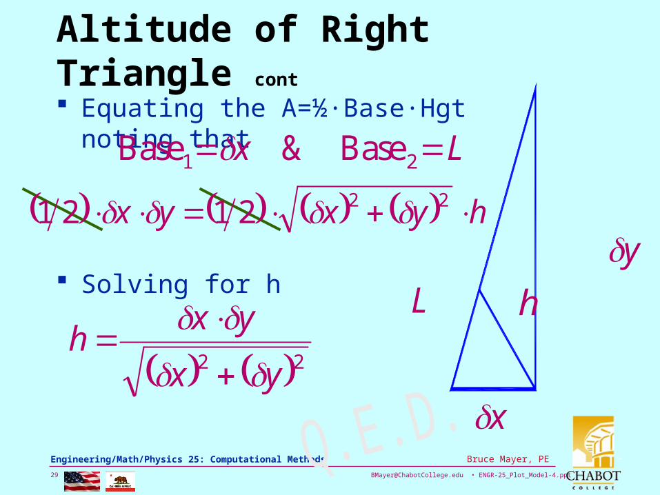
Altitude of Right Triangle cont
y
x
L h
hyxyx 222121
Solving for h
22 yx
yxh
Lx 21 Base&Base Equating the A=½·Base·Hgt noting that
[email protected] • ENGR-25_Plot_Model-4.ppt30
Bruce Mayer, PE Engineering/Math/Physics 25: Computational Methods
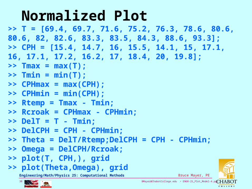
Normalized Plot>> T = [69.4, 69.7, 71.6, 75.2, 76.3, 78.6, 80.6, 80.6, 82, 82.6, 83.3, 83.5, 84.3, 88.6, 93.3];>> CPH = [15.4, 14.7, 16, 15.5, 14.1, 15, 17.1, 16, 17.1, 17.2, 16.2, 17, 18.4, 20, 19.8];>> Tmax = max(T);>> Tmin = min(T);>> CPHmax = max(CPH);>> CPHmin = min(CPH);>> Rtemp = Tmax - Tmin;>> Rcroak = CPHmax - CPHmin;>> DelT = T - Tmin;>> DelCPH = CPH - CPHmin;>> Theta = DelT/Rtemp;DelCPH = CPH - CPHmin;>> Omega = DelCPH/Rcroak;>> plot(T, CPH,), grid>> plot(Theta,Omega), grid
[email protected] • ENGR-25_Plot_Model-4.ppt31
Bruce Mayer, PE Engineering/Math/Physics 25: Computational Methods
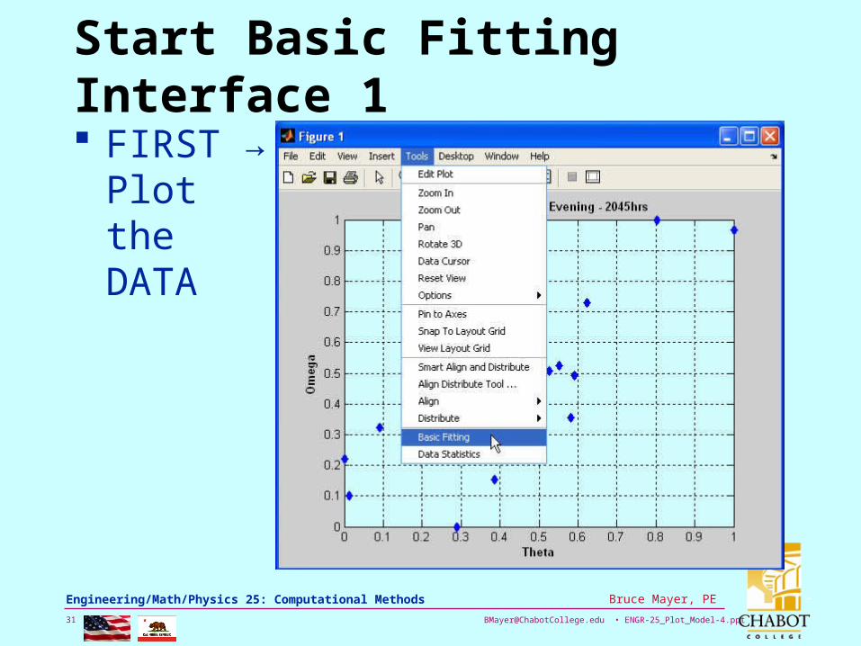
Start Basic Fitting Interface 1
FIRST → Plot the DATA
[email protected] • ENGR-25_Plot_Model-4.ppt32
Bruce Mayer, PE Engineering/Math/Physics 25: Computational Methods
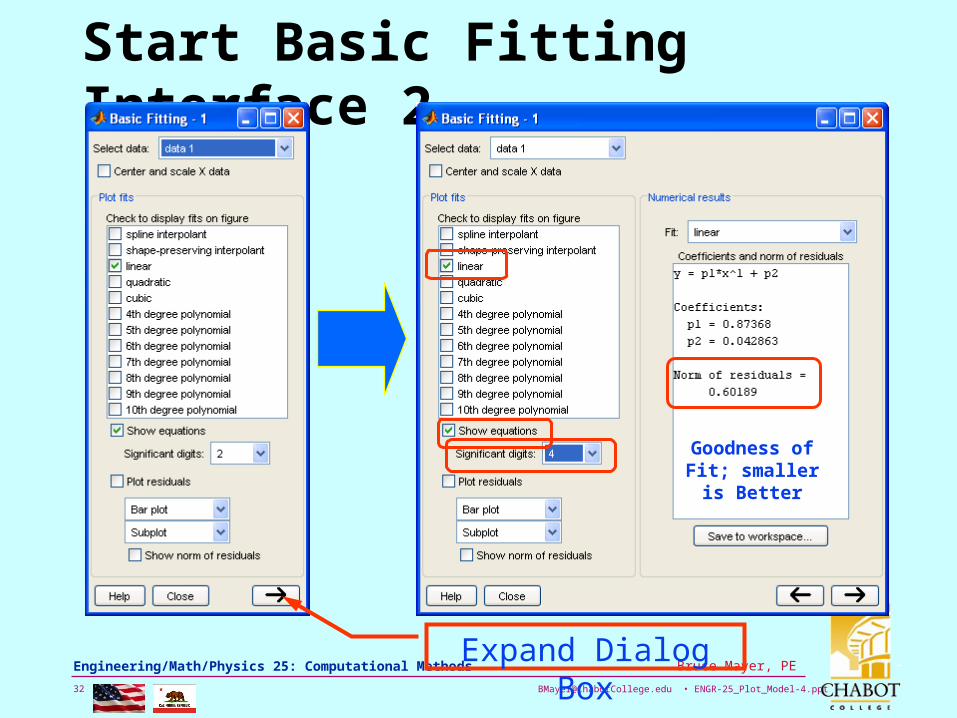
Start Basic Fitting Interface 2
Expand Dialog Box
Goodness of Fit; smaller is
Better
[email protected] • ENGR-25_Plot_Model-4.ppt33
Bruce Mayer, PE Engineering/Math/Physics 25: Computational Methods
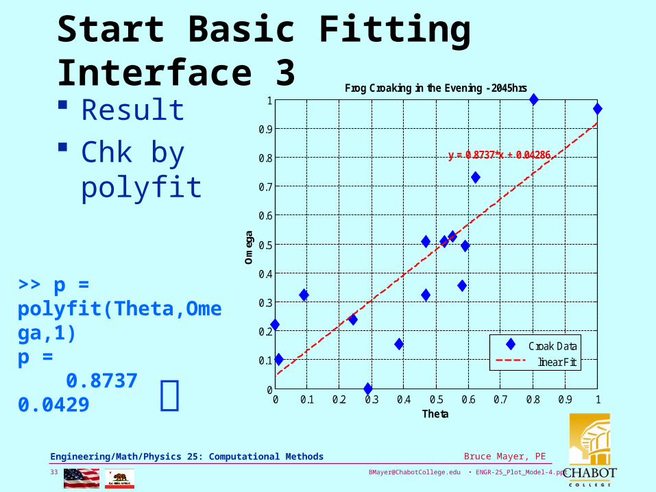
Start Basic Fitting Interface 3
Result Chk by
polyfit
0 0.1 0.2 0.3 0.4 0.5 0.6 0.7 0.8 0.9 10
0.1
0.2
0.3
0.4
0.5
0.6
0.7
0.8
0.9
1
Theta
Om
ega
Frog Croaking in the Evening - 2045hrs
y = 0.8737*x + 0.04286
Croak Data
linear Fit
>> p = polyfit(Theta,Omega,1)p = 0.8737 0.0429
[email protected] • ENGR-25_Plot_Model-4.ppt34
Bruce Mayer, PE Engineering/Math/Physics 25: Computational Methods
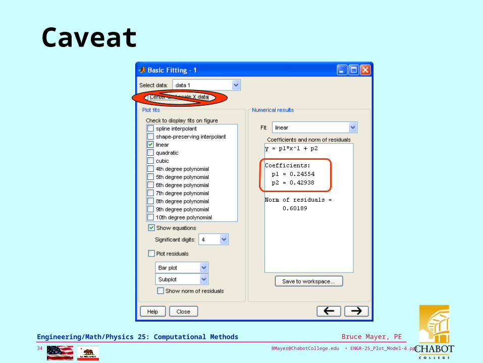
Caveat
[email protected] • ENGR-25_Plot_Model-4.ppt35
Bruce Mayer, PE Engineering/Math/Physics 25: Computational Methods
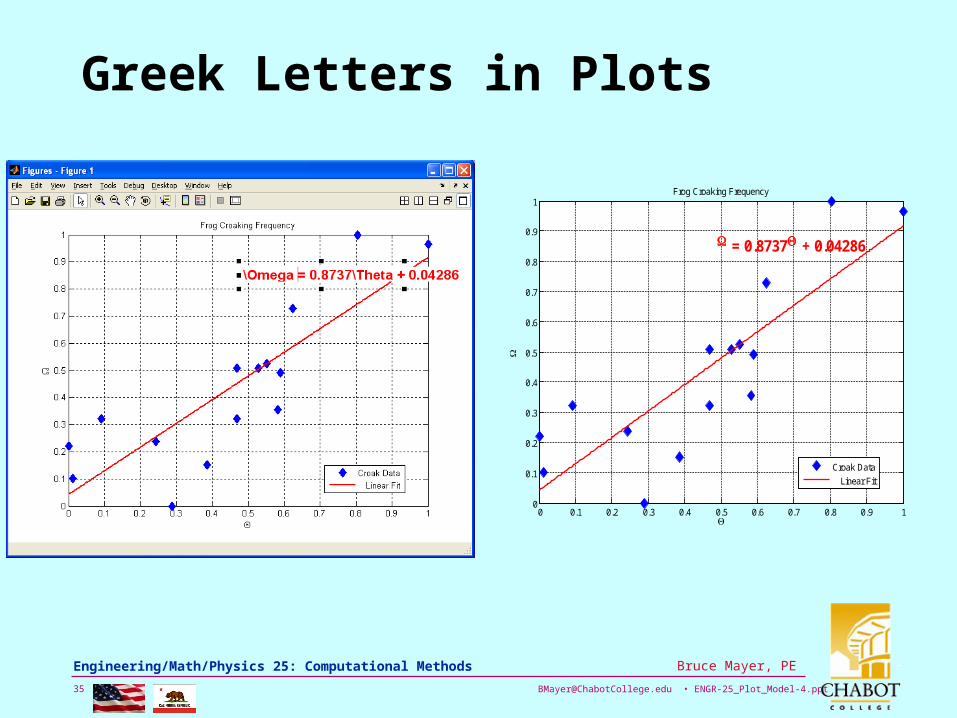
Greek Letters in Plots
0 0.1 0.2 0.3 0.4 0.5 0.6 0.7 0.8 0.9 10
0.1
0.2
0.3
0.4
0.5
0.6
0.7
0.8
0.9
1Frog Croaking Frequency
Croak Data
Linear Fit
= 0.8737 + 0.04286
[email protected] • ENGR-25_Plot_Model-4.ppt36
Bruce Mayer, PE Engineering/Math/Physics 25: Computational Methods
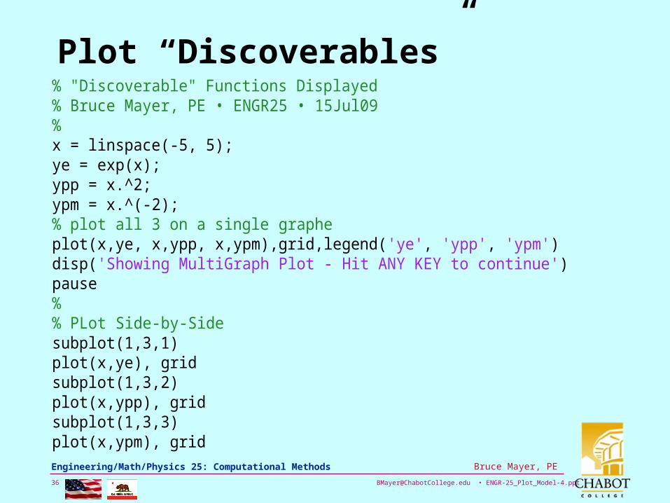
Plot “Discoverables”% "Discoverable" Functions Displayed% Bruce Mayer, PE • ENGR25 • 15Jul09%x = linspace(-5, 5);ye = exp(x);ypp = x.^2;ypm = x.^(-2);% plot all 3 on a single grapheplot(x,ye, x,ypp, x,ypm),grid,legend('ye', 'ypp', 'ypm')disp('Showing MultiGraph Plot - Hit ANY KEY to continue')pause%% PLot Side-by-Sidesubplot(1,3,1)plot(x,ye), gridsubplot(1,3,2)plot(x,ypp), gridsubplot(1,3,3)plot(x,ypm), grid
[email protected] • ENGR-25_Plot_Model-4.ppt37
Bruce Mayer, PE Engineering/Math/Physics 25: Computational Methods
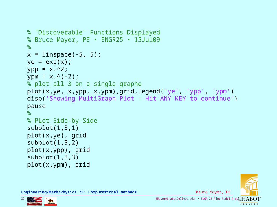
% "Discoverable" Functions Displayed% Bruce Mayer, PE • ENGR25 • 15Jul09%x = linspace(-5, 5);ye = exp(x);ypp = x.^2;ypm = x.^(-2);% plot all 3 on a single grapheplot(x,ye, x,ypp, x,ypm),grid,legend('ye', 'ypp', 'ypm')disp('Showing MultiGraph Plot - Hit ANY KEY to continue')pause%% PLot Side-by-Sidesubplot(1,3,1)plot(x,ye), gridsubplot(1,3,2)plot(x,ypp), gridsubplot(1,3,3)plot(x,ypm), grid
Recommended