T. Brinker, E. D. Ellen, R. F. Veerkamp, P. Bijma
Breeding Value Predictions for Survival
in Laying Hens Showing Cannibalism
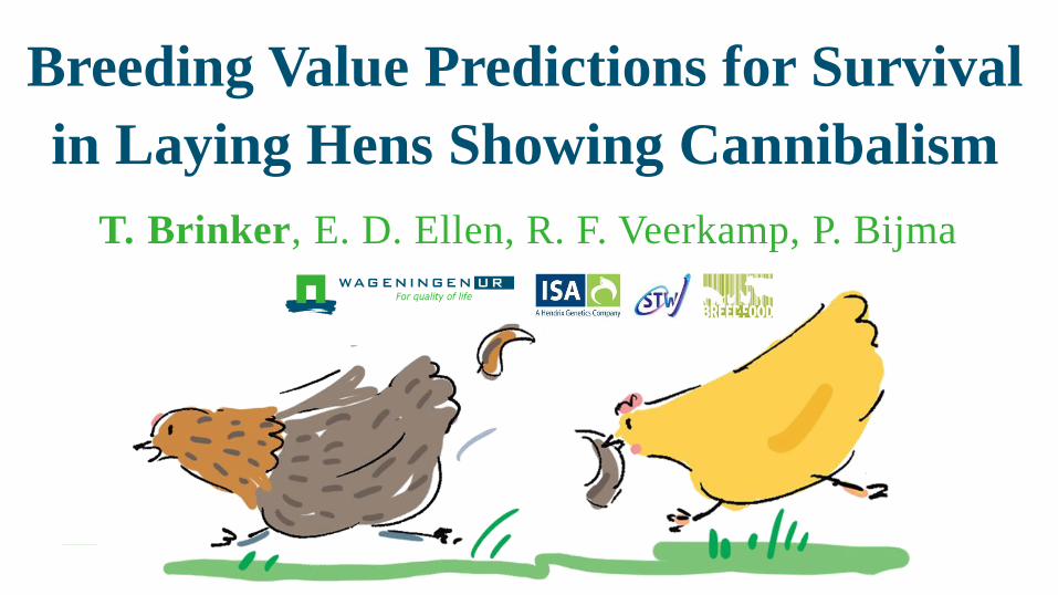
Feather Pecking Feather pecking and cannibalism
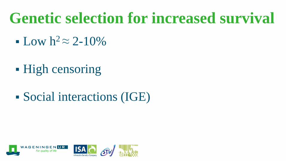
Genetic selection for increased survival
Low h2 ≈ 2-10%
High censoring
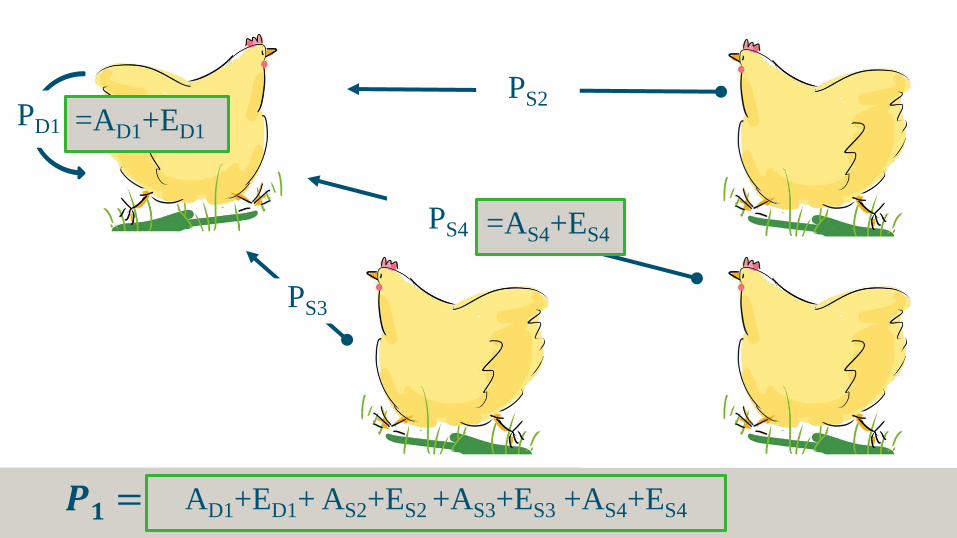
Social interactions (IGE)
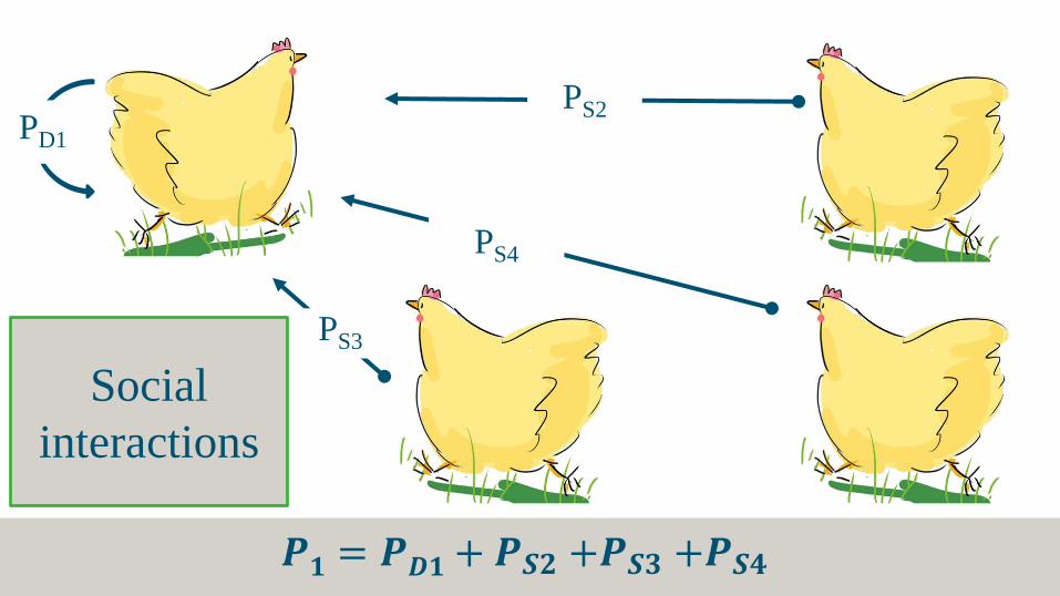
PS3
PD1
PS2
PS4
𝑷𝟏 = 𝑷𝑫𝟏+ 𝑷𝑺𝟐 +𝑷𝑺𝟑 +𝑷𝑺𝟒
Social
interactions
PS3
PD1
PS2
PS4
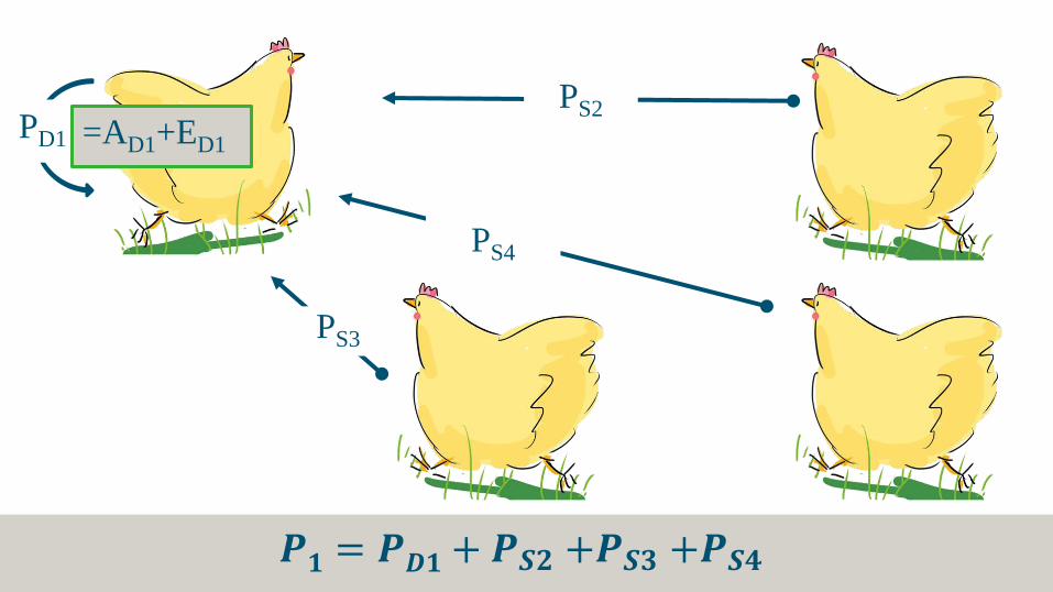
𝑷𝟏 = 𝑷𝑫𝟏+ 𝑷𝑺𝟐 +𝑷𝑺𝟑 +𝑷𝑺𝟒
=AD1+ED1
PS3
PD1
PS2
PS4
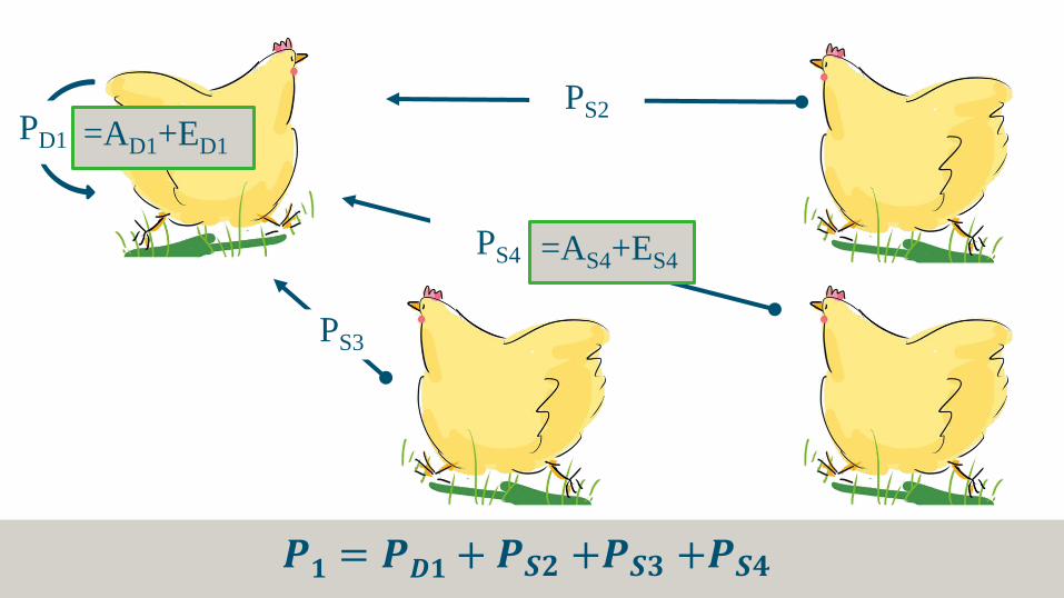
𝑷𝟏 = 𝑷𝑫𝟏+ 𝑷𝑺𝟐 +𝑷𝑺𝟑 +𝑷𝑺𝟒
=AS4+ES4
=AD1+ED1
PS3
PD1
PS2
PS4
𝑷𝟏 = 𝑷𝑫𝟏+ 𝑷𝑺𝟐 +𝑷𝑺𝟑 +𝑷𝑺𝟒
=AS4+ES4
AD1+ED1+ AS2+ES2 +AS3+ES3 +AS4+ES4
=AD1+ED1
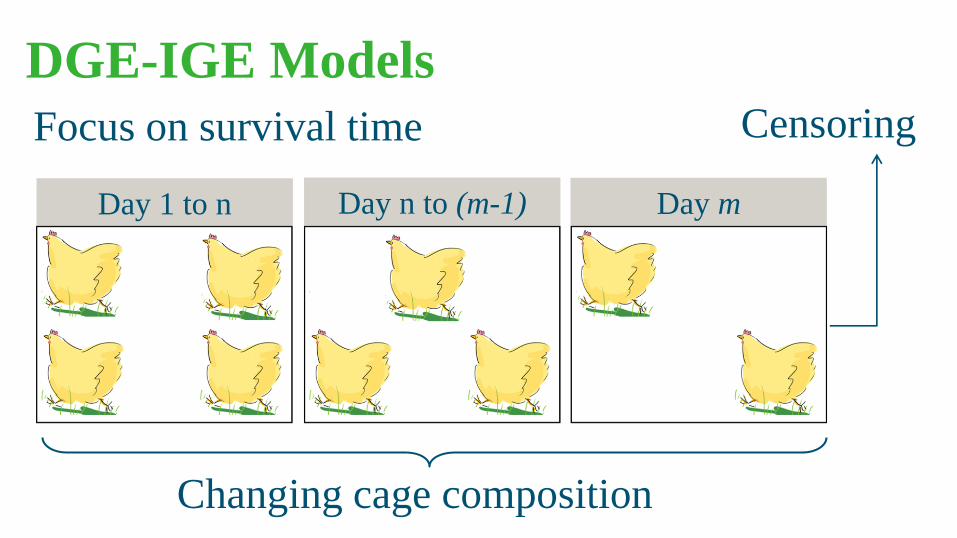
Focus on survival time
DGE-IGE Models
Day m Day n to (m-1) Day 1 to n
Changing cage composition
Censoring
Objective
Improve breeding value predictions for
survival time in laying hens showing
cannibalism

DATA

2 purebred White Leghorn layer lines
6 276 W1
6 916 WB
Intact beaks
Genetic stock
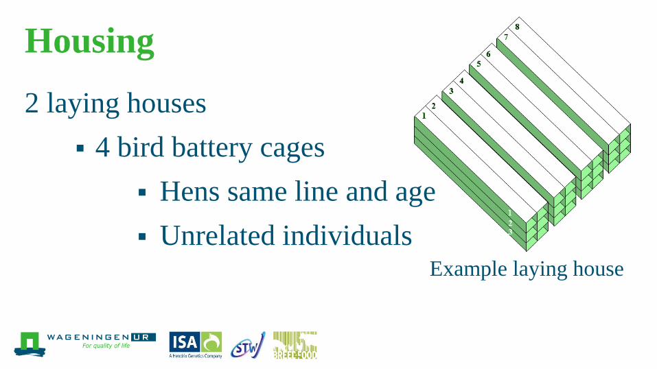
Housing
2 laying houses
4 bird battery cages
Hens same line and age
Unrelated individuals
Example laying house
Data collection
Survival Time
Survival each month (max=13)
alive (1) or dead (0)

METHODS
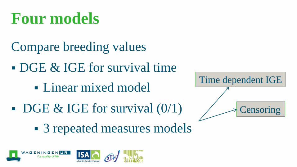
Four models
Compare breeding values
DGE & IGE for survival time
Linear mixed model
DGE & IGE for survival (0/1)
3 repeated measures models
Censoring
Time dependent IGE
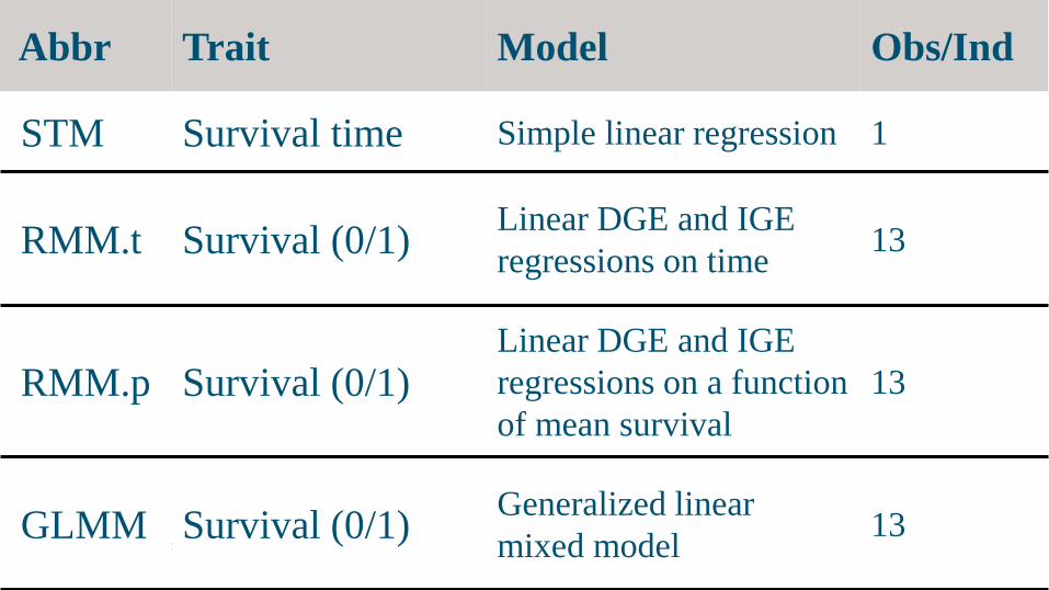
Abbr Trait Model Obs/Ind
STM Survival time Simple linear regression 1
RMM.t Survival (0/1) Linear DGE and IGE
regressions on time 13
RMM.p Survival (0/1) Linear DGE and IGE
regressions on a function
of mean survival
13
GLMM Survival (0/1) Generalized linear
mixed model 13
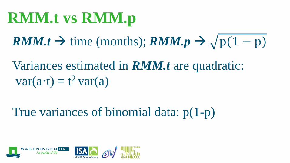
RMM.t vs RMM.p
RMM.t time (months); RMM.p p(1 − p)
Variances estimated in RMM.t are quadratic:
var(a·t) = t2 var(a)
True variances of binomial data: p(1-p)
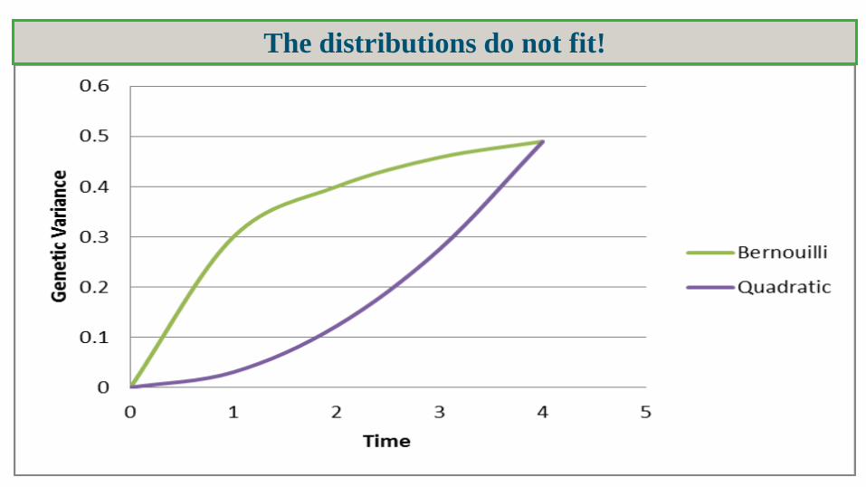
Models – RMM.p Model The distributions do not fit!
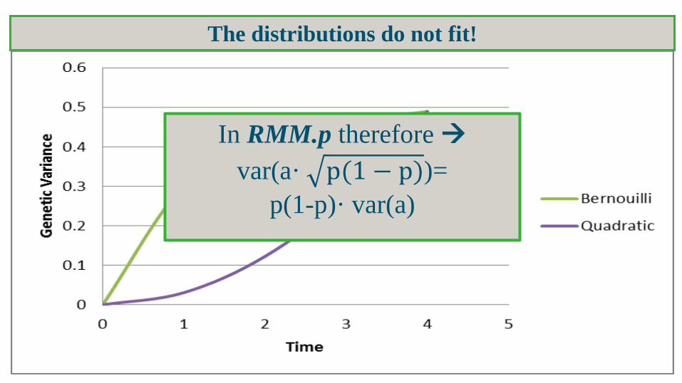
Models – RMM.p Model The distributions do not fit!
In RMM.p therefore
var(a· p(1 − p))=
p(1-p)· var(a)
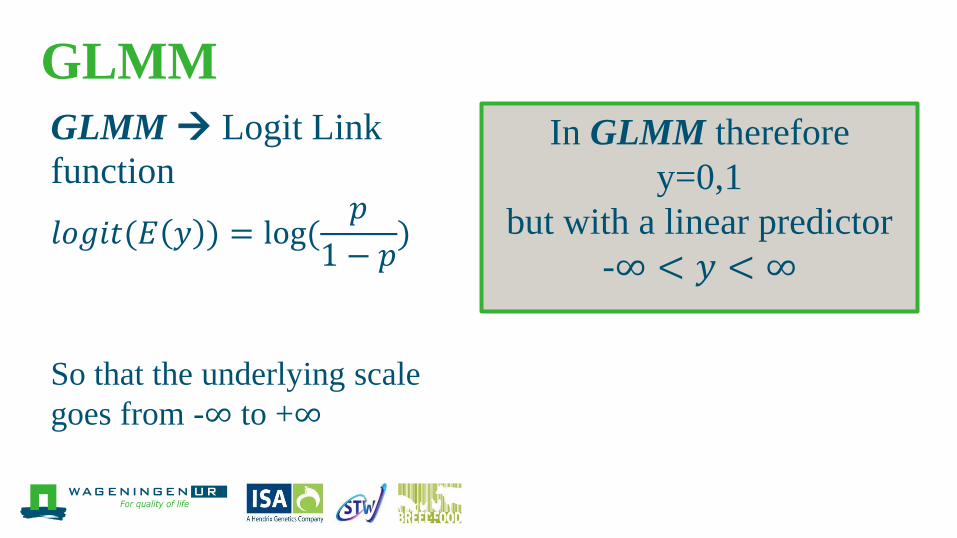
GLMM
𝑙𝑜𝑔𝑖𝑡(𝐸 𝑦 ) = log(𝑝
1 − 𝑝)
So that the underlying scale
goes from -∞ to +∞
GLMM Logit Link
function In GLMM therefore
y=0,1
but with a linear predictor
-∞ < 𝑦 < ∞
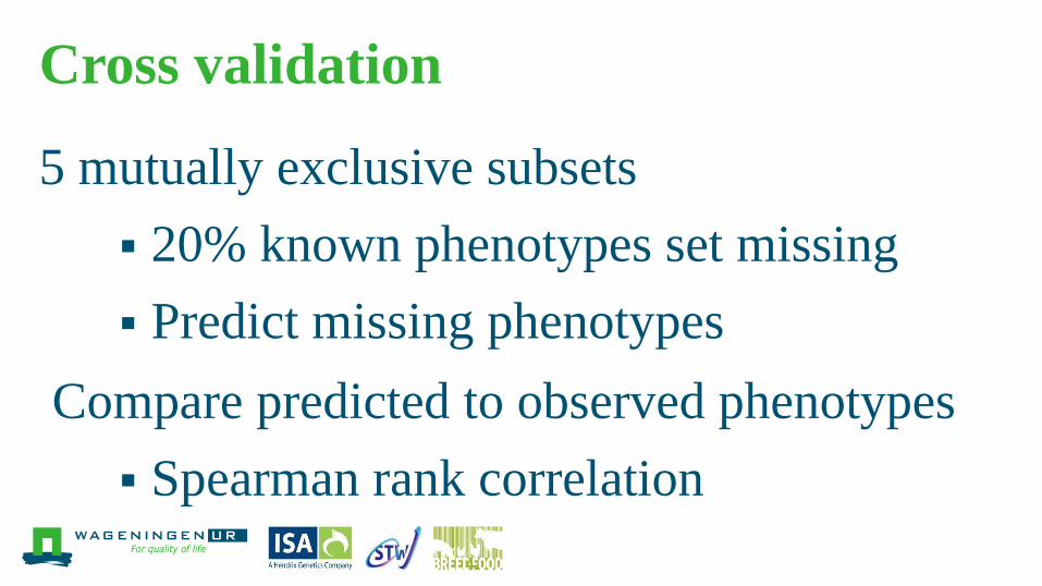
Cross validation
5 mutually exclusive subsets
20% known phenotypes set missing
Predict missing phenotypes
Compare predicted to observed phenotypes
Spearman rank correlation

RESULTS
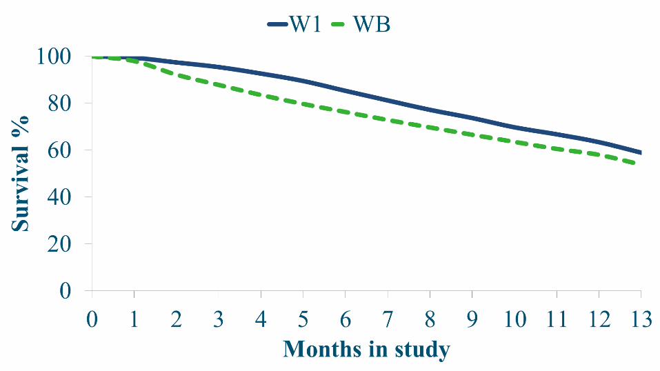
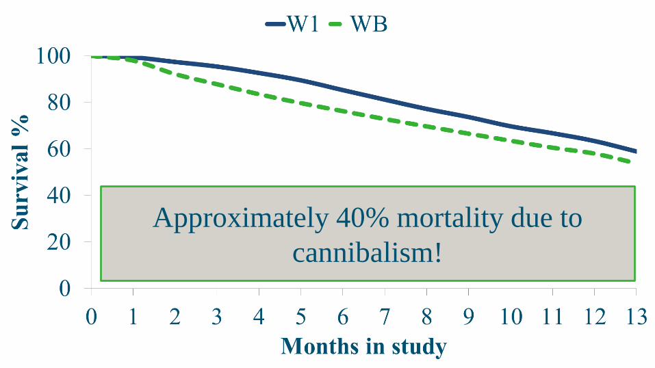
Approximately 40% mortality due to
cannibalism!
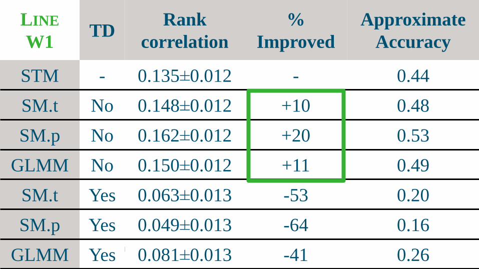
LINE
W1 TD
Rank
correlation
%
Improved
Approximate
Accuracy
STM - 0.135±0.012 - 0.44
SM.t No 0.148±0.012 +10 0.48
SM.p No 0.162±0.012 +20 0.53
GLMM No 0.150±0.012 +11 0.49
SM.t Yes 0.063±0.013 -53 0.20
SM.p Yes 0.049±0.013 -64 0.16
GLMM Yes 0.081±0.013 -41 0.26
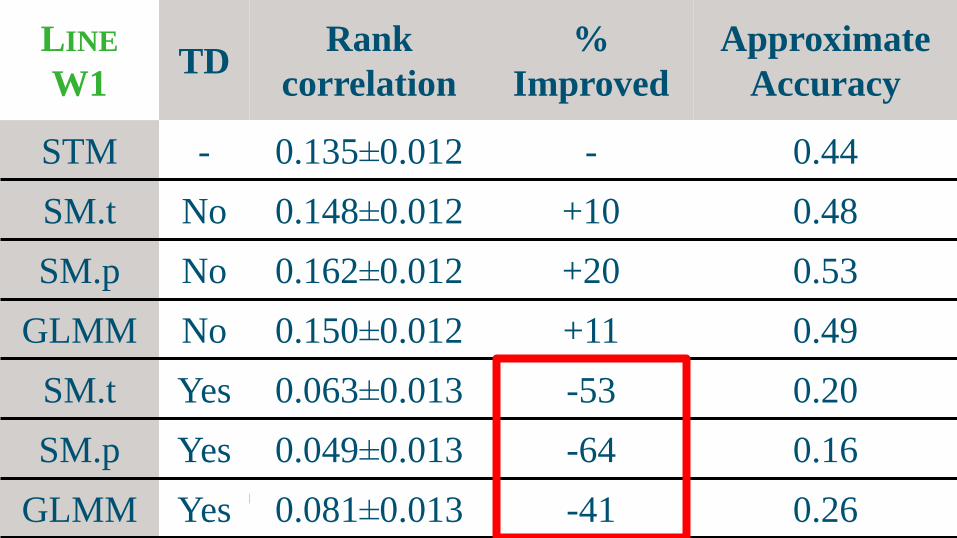
LINE
W1 TD
Rank
correlation
%
Improved
Approximate
Accuracy
STM - 0.135±0.012 - 0.44
SM.t No 0.148±0.012 +10 0.48
SM.p No 0.162±0.012 +20 0.53
GLMM No 0.150±0.012 +11 0.49
SM.t Yes 0.063±0.013 -53 0.20
SM.p Yes 0.049±0.013 -64 0.16
GLMM Yes 0.081±0.013 -41 0.26
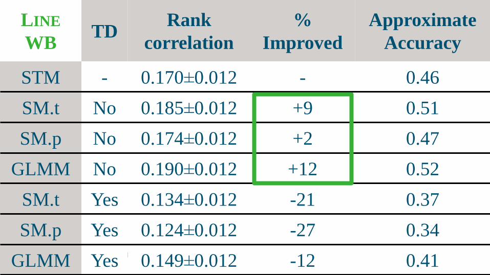
LINE
WB TD
Rank
correlation
%
Improved
Approximate
Accuracy
STM - 0.170±0.012 - 0.46
SM.t No 0.185±0.012 +9 0.51
SM.p No 0.174±0.012 +2 0.47
GLMM No 0.190±0.012 +12 0.52
SM.t Yes 0.134±0.012 -21 0.37
SM.p Yes 0.124±0.012 -27 0.34
GLMM Yes 0.149±0.012 -12 0.41
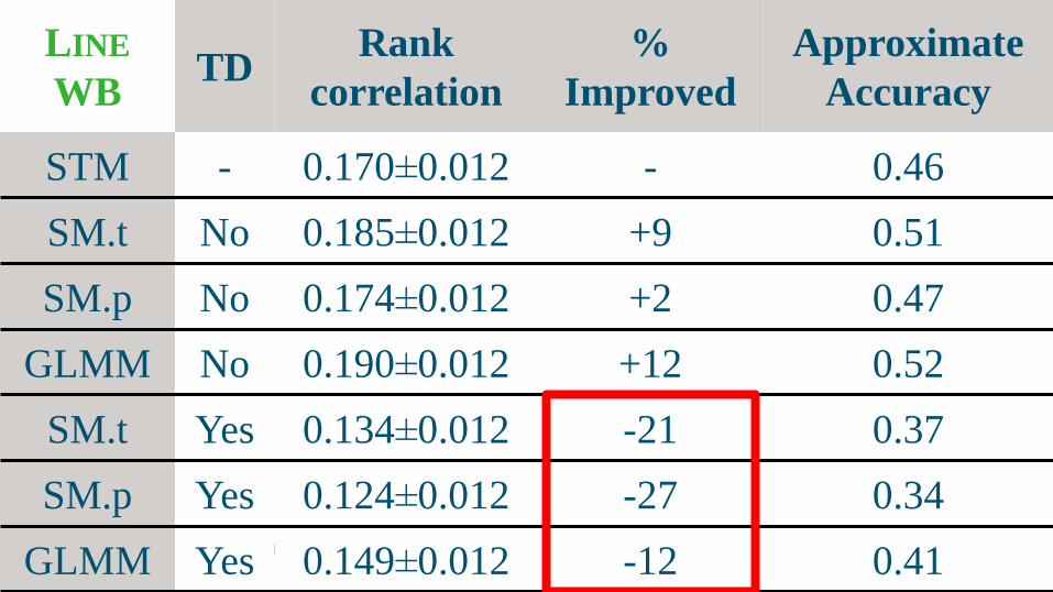
LINE
WB TD
Rank
correlation
%
Improved
Approximate
Accuracy
STM - 0.170±0.012 - 0.46
SM.t No 0.185±0.012 +9 0.51
SM.p No 0.174±0.012 +2 0.47
GLMM No 0.190±0.012 +12 0.52
SM.t Yes 0.134±0.012 -21 0.37
SM.p Yes 0.124±0.012 -27 0.34
GLMM Yes 0.149±0.012 -12 0.41
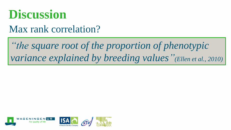
Discussion
“the square root of the proportion of phenotypic
variance explained by breeding values”(Ellen et al., 2010)
Max rank correlation?
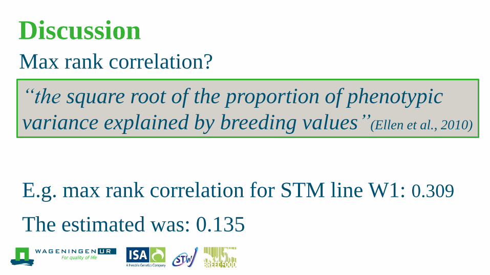
Discussion
“the square root of the proportion of phenotypic
variance explained by breeding values”(Ellen et al., 2010)
E.g. max rank correlation for STM line W1: 0.309
The estimated was: 0.135
Max rank correlation?
Discussion
Improvement of models because of censoring
issue
Time dependent IGE are detrimental
Discussion
Improvement of models because of censoring
issue
Time dependent IGE are detrimental
Lipschutz-Powell et al. (2012) adjusted the IGE
model; infected individuals only express IGE on
susceptible group mates.
Conclusion
Using repeated measurement models, accuracies
of EBVs were improved
10%-20% in W1
9%-12% in WB
Implication: response to selection can be improved
accordingly
Conclusion
Using repeated measurement models, accuracies
of EBVs were improved
10%-20% in W1
9%-12% in WB
Implication: response to selection can be improved
accordingly
Thank you!

EXTRA SLIDES
What are the genetic parameters?
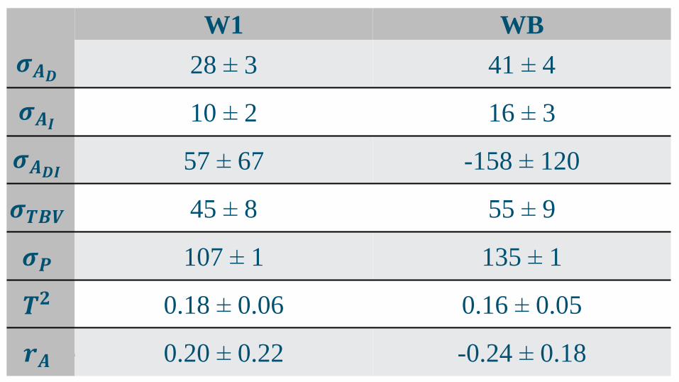
W1 WB
𝝈𝑨𝑫 28 ± 3 41 ± 4
𝝈𝑨𝑰 10 ± 2 16 ± 3
𝝈𝑨𝑫𝑰 57 ± 67 -158 ± 120
𝝈𝑻𝑩𝑽 45 ± 8 55 ± 9
𝝈𝑷 107 ± 1 135 ± 1
𝑻𝟐 0.18 ± 0.06 0.16 ± 0.05
𝒓𝑨 0.20 ± 0.22 -0.24 ± 0.18
How to model time dependent IGE?
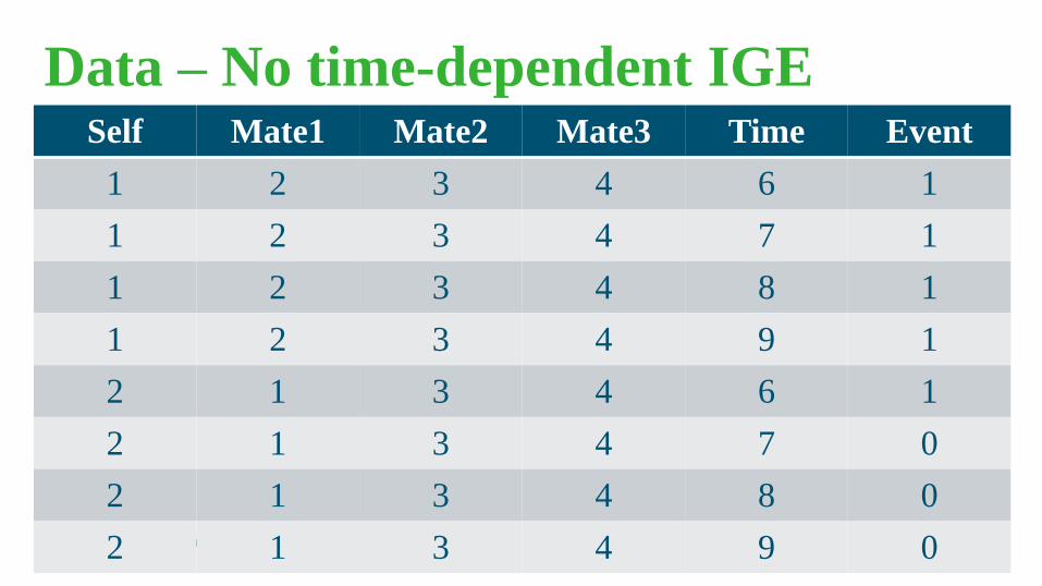
Data – No time-dependent IGE Self Mate1 Mate2 Mate3 Time Event
1 2 3 4 6 1
1 2 3 4 7 1
1 2 3 4 8 1
1 2 3 4 9 1
2 1 3 4 6 1
2 1 3 4 7 0
2 1 3 4 8 0
2 1 3 4 9 0
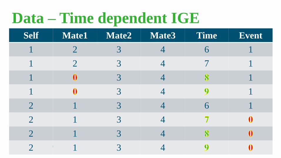
Data – Time dependent IGE Self Mate1 Mate2 Mate3 Time Event
1 2 3 4 6 1
1 2 3 4 7 1
1 3 4 1
1 3 4 1
2 1 3 4 6 1
2 1 3 4
2 1 3 4
2 1 3 4

How do the models look like?
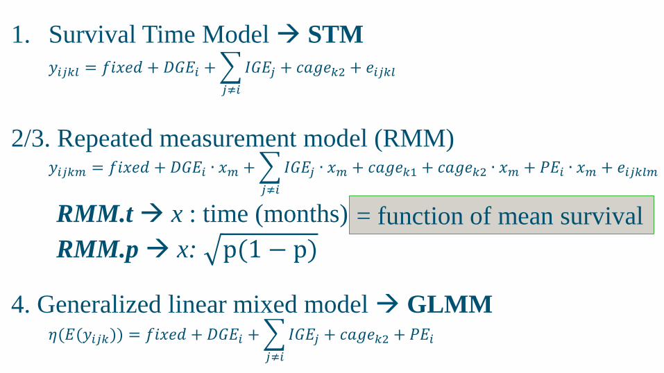
1. Survival Time Model STM
2/3. Repeated measurement model (RMM)
RMM.t x : time (months)
RMM.p x: p(1 − p)
4. Generalized linear mixed model GLMM
𝑦𝑖𝑗𝑘𝑚 = 𝑓𝑖𝑥𝑒𝑑 + 𝐷𝐺𝐸𝑖 ∙ 𝑥𝑚 + 𝐼𝐺𝐸𝑗 ∙ 𝑥𝑚𝑗≠𝑖
+ 𝑐𝑎𝑔𝑒𝑘1 + 𝑐𝑎𝑔𝑒𝑘2 ∙ 𝑥𝑚 + 𝑃𝐸𝑖 ∙ 𝑥𝑚 + 𝑒𝑖𝑗𝑘𝑙𝑚
𝑦𝑖𝑗𝑘𝑙 = 𝑓𝑖𝑥𝑒𝑑 + 𝐷𝐺𝐸𝑖 + 𝐼𝐺𝐸𝑗𝑗≠𝑖
+ 𝑐𝑎𝑔𝑒𝑘2 + 𝑒𝑖𝑗𝑘𝑙
𝜂(𝐸(𝑦𝑖𝑗𝑘)) = 𝑓𝑖𝑥𝑒𝑑 + 𝐷𝐺𝐸𝑖 + 𝐼𝐺𝐸𝑗𝑗≠𝑖
+ 𝑐𝑎𝑔𝑒𝑘2 + 𝑃𝐸𝑖
= function of mean survival
How do you calculate observed
phenotypes?
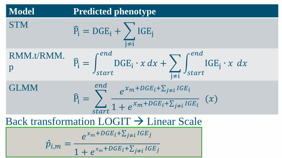
Model Predicted phenotype
STM P i = DGEi + IGEj
j≠i
RMM.t/RMM.
p P i = DGEi ∙ 𝑥𝑒𝑛𝑑
𝑠𝑡𝑎𝑟𝑡
𝑑𝑥 + IGEj ∙ 𝑥𝑒𝑛𝑑
𝑠𝑡𝑎𝑟𝑡j≠i
𝑑𝑥
GLMM
P i = 𝑒𝑥𝑚+𝐷𝐺𝐸𝑖+ 𝐼𝐺𝐸𝑖𝑗≠𝑖
1 + 𝑒𝑥𝑚+𝐷𝐺𝐸𝑖+ 𝐼𝐺𝐸𝑖𝑗≠𝑖
𝑒𝑛𝑑
𝑠𝑡𝑎𝑟𝑡
(𝑥)
𝑝 𝑖,𝑚 =𝑒𝑥𝑚+𝐷𝐺𝐸𝑖+ 𝐼𝐺𝐸𝑗𝑗≠𝑖
1 + 𝑒𝑥𝑚+𝐷𝐺𝐸𝑖+ 𝐼𝐺𝐸𝑗𝑗≠𝑖
Back transformation LOGIT Linear Scale

How do you calculate the max
correlation?
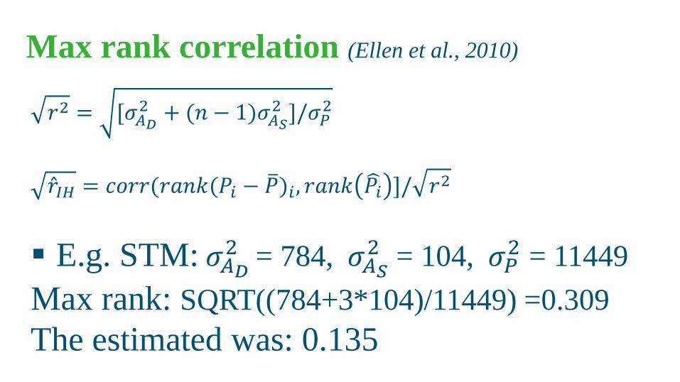
Max rank correlation (Ellen et al., 2010)
𝑟2 = [𝜎𝐴𝐷2 + (𝑛 − 1)𝜎𝐴𝑆
2 ]/𝜎𝑃2
𝑟 𝐼𝐻 = 𝑐𝑜𝑟𝑟(𝑟𝑎𝑛𝑘(𝑃𝑖 − 𝑃 )𝑖 , 𝑟𝑎𝑛𝑘 𝑃𝑖 ]/ 𝑟2
E.g. STM:𝜎𝐴𝐷2 = 784, 𝜎𝐴𝑆
2 = 104, 𝜎𝑃2 = 11449
Max rank: SQRT((784+3*104)/11449) =0.309
The estimated was: 0.135
Recommended