Budget Deficits and Exchange-Rate Crises∗
Barbara Annicchiarico† Giancarlo Marini‡
Giovanni Piersanti§
May 2007
Abstract
This paper investigates currency crises in an optimizing general
equilibrium model with overlapping generations. It is shown that a
rise in government budget deficits financed by future taxes generates a
decumulation of external assets, leading up to a speculative attack and
forcing the monetary authorities to abandon the peg.
JEL classification: F31; F32; F41; E52; E62.
Keywords: budget deficits, foreign exchange reserves, currency crises.
∗We wish to thank Fabio C. Bagliano, Marianne Baxter, Leonardo Becchetti, LorenzoBini Smaghi, Giancarlo Corsetti, Alberto Dalmazzo, Bassam Fattouh, Laurence Harris,Fabrizio Mattesini, Pedro M. Oviedo, Alberto Petrucci, Alessandro Piergallini, Cristina M.Rossi, Pasquale Scaramozzino and Salvatore Vinci for helpful comments and suggestionson a previous version of this paper.
†Corresponding Author : Assistant Professor of Economics. Department of Eco-nomics, University of Rome “Tor Vergata”, Via Columbia 2, 00133 Roma, Italy. Phone:+390672595731; Fax: +39062020500. E-mail address: [email protected].
‡Professor of Economics. Department of Economics, University of Rome “Tor Vergata”.§Professor of Economics. University of Rome “Tor Vergata” and University of Teramo.
Discussion Paper 73
The Centre for Financial and Management Studies
1 Introduction
The financial and currency turmoils of the 90’s in many European, Latin-
American and Asian countries have called into question the viability of fixed
exchange-rate regimes and led to the development of new models on the causes
of currency collapses. We can now identify at least two main theoretical ex-
planations of crises, one based on the view that a collapse is the inevitable
outcome of inconsistent macroeconomic policies and the other based on the
view that a collapse results from self-fulfilling expectations. According to the
so-called ‘first-generation’ models of currency crises, if a government finances
its fiscal deficits by printing money in excess of money demand growth, while
following a fixed exchange-rate policy, a gradual loss of reserves will occur,
leading to a speculative attack against the currency that forces the abandon-
ment of the fixed-rate regime eventually (see, e.g., Krugman 1979; Flood and
Garber 1984; Obstfled 1986a; Calvo 1987; van Wijnbergen 1991; Calvo and
Vegh 1999).
The ‘second-generation’ models of currency crises, on the other hand, show
that the government’s decision to give up a fixed exchange rate depends on the
net benefits of pegging; hence, the fixed rate is likely to be maintained as long
as the benefits of devaluing are smaller than the costs. However, changes in
market beliefs about the currency sustainability can force the government to
go out of the peg. For example, if agents expect a devaluation, a speculative
attack will start, forcing the government to abandon the peg, since the costs
of keeping the exchange rate fixed outweigh the benefits. On the other hand,
if agents expect no change in the currency rate the fixed peg will be preserved.
Private expectations are self-fulfilling and multiple equilibria can occur, for
given fundamentals (see, e.g., Obstfeld 1996; Velasco 1996; Cole and Kehoe
1996; Jeanne 1997; Jeanne and Masson, 2000).1
1The partition between first and second generation models is consistent with the classifi-cation scheme of currency crises proposed by Flood and Marion (1999), and Jeanne (2000).From this point of view the so called “third-generation” models, elaborated to explain themore recent financial turmoils in Asia, Latin America and Russia, are considered extensionsof the existing setups that explicitly include the financial side of the economy.
1
Budget Deficits and Exchange-Rate Crises
SOAS, University of London
More recently, the debate about the role played by fundamentals and/or
self-fulfilling expectations in triggering a speculative attack has been enriched
by a new set of models analyzing currency crises in the context of a change
in the expectations of future policy (see, e.g., Daniel 2000, 2001; Burnside,
Eichenbaum, and Rebelo 2001, 2003). According to this view, explanations of
crises do not necessarily require a period of fundamental misalignments. All
is needed is that the path of current and future government policies becomes
inconsistent with the fixed peg.
This literature typically uses static models, or models with extrinsic dy-
namics, that is models where the dynamics of the system come exclusively
from current or anticipated future changes in exogenous variables. Such sys-
tems are, in fact, always in steady-state equilibrium in the absence of external
shocks. This is in contrast to the so-called intrinsic dynamics of the system,
where the economy evolves from some initial stationary state due to, e.g., the
accumulation of capital stock or foreign assets.2 Models with intrinsic dynam-
ics are useful to understand currency crises and to predict the exact time of
an attack. They enable us to study the dynamics of relevant macroeconomic
variables.
The purpose of this paper is to deal with this kind of dynamics using a
modified version of the Yaari (1965)-Blanchard (1985) model. Our approach
has three main advantages. First, it allows a ‘nondegenerate’ dynamic adjust-
ment in the basic monetary model of exchange rate determination. Second,
it shows that the macroeconomic equilibrium is dependent on the timing of
fiscal policies. Third, the current account is allowed to play a crucial role in
transmitting fiscal disturbances to the rest of the economy.
A central finding of the paper is that a collapse may occur even as a con-
sequence of a temporary tax cut fully financed by future taxes. In particular,
following a fiscal expansion, current account imbalances and the expected
depletion of foreign assets will lead up to a currency crisis forcing the mon-
2This distinction may be found, for example, in Turnovsky (1977, 1997) and Obstfeldand Stockman (1985).
2
Discussion Paper 73
The Centre for Financial and Management Studies
etary authorities to adopt a floating exchange-rate regime. This result is in
sharp contrast with the existing literature, where monetary or fiscal policies
are inconsistent or expected to be inconsistent with the exchange-rate policy.
On the other hand, our theoretical results are consistent with the evidence
that Asian countries that came under attack in 1997 were those which had
experienced lager current account deficits on the eve of the crisis.3
The main conclusion that emerges from our analysis is that crises can occur
in a flexible price fully optimizing framework even when both monetary and
fiscal policies are correctly designed, that is when the intertemporal budget
constraint of the government is always respected and monetary policy obeys
the rules of the game. The crisis, however, is not driven by self-fulfilling expec-
tations, as the collapse results from a well-defined dynamics in the fundamen-
tals. The main implication of our model is that the sustainability of a fixed
exchange-rate system may require not only giving up monetary sovereignty,
but also strongly restraining the conduct of fiscal policy.
The paper is organized as follows. Section II presents the theoretical
model. Section III describes the dynamics of the model and the time of the
speculative attack. Section IV contains the summary and conclusions of the
paper.
2 The Model
Consider a small open economy described as follows. Agents have perfect
foresight and consume a single tradeable good. Domestic supply of the good
is exogenous. Household’s financial wealth is divided between domestic money
(which is not held abroad) and internationally traded bonds. There are no
barriers to trade, so that purchasing power parity (ppp) holds at all times,
that is P ∗S = P , where S is the nominal exchange rate (defined as units
of domestic currency per unit of foreign currency), P is the domestic price
3For an exhaustive overview of the economic fundamentals in Asian countries in theyears preceding the financial and currency crisis, see Corsetti, Pesenti and Roubini (1999)and World Bank (1999).
3
Budget Deficits and Exchange-Rate Crises
SOAS, University of London
level and P ∗ is the foreign price level. There is perfect capital mobility and
domestic and foreign assets are perfect substitutes, thus uncovered interest
parity (uip) is always verified, i = i∗ + s, where i and i∗ are the domestic
and foreign (constant) nominal interest rate, respectively and s ≡ d (ln S) /dt
is the rate of exchange depreciation. In the absence of foreign inflation the
external nominal interest rate is equal to the real rate.
The demand side of the economy is described by an extended version of the
Yaari-Blanchard perpetual youth model with money in the utility function.4
There is no bequest motive and financial wealth for newly born agents is
assumed to be zero. The birth and death rates are the same, so that population
is constant. Let δ denote the instantaneous constant probability of death and
β the subjective discount rate. For convenience, the size of each generation
at birth is normalized to δ, hence total population is equal to unity.
Each individual of the generation born at time s at each time period t ≥ s
faces the following maximization problem:
max
∫∞
0
log
(cǫs,t
ms,t
Pt
1−ǫ)
e−(β+δ)tdt, (1)
subject to the individual consumer’s flow budget constraint
d (ws,t/Pt)
dt= (i∗ − p∗t + δ)
ws,t
Pt
+ ys,t − τ s,t − cs,t − (i∗ + st)ms,t
Pt
, (2)
and to the transversality condition
limt→∞
ws,t
Pt
e−∫ t0(i∗−p∗υ+δ)dυ = 0, (3)
where 0 < ǫ < 1, β < i∗− p∗,5 p∗ is the external inflation rate, while cs, ys, ms,
ws and τ s denote consumption, endowment, nominal money balances, total
4The approach of entering money in the utility function to allow for money holdingbehavior within a Yaari-Blanchard framework, is common to a number of papers includingSpaventa (1987), Marini and van der Ploeg (1988), van der Ploeg (1991), and Kawai andMaccini (1990, 1995). Similar results could also be obtained by use of cash-in-advancemodels (see Feenstra, 1986).
5Following Blanchard (1985) this condition ensures that consumers are relatively patient,in order to ensure that the steady state-level of aggregate financial wealth is positive.
4
Discussion Paper 73
The Centre for Financial and Management Studies
financial wealth and lump-sum taxes, respectively. Notice that the effective
discount rate of consumers is given by β + δ, where β + δ > i∗ − p∗.6 Each
individual is assumed to receive for every period of her life an actuarial fair
premium equal to a fraction δ of her financial wealth from a life insurance
company operating in a perfectly competitive market. At the time of her
death the remaining individual’s net wealth goes to the insurance company.
For simplicity, both the endowment and the amount of lump-sum taxes are
age-independent; hence, individuals of all generations have the same human
wealth. In addition, the endowment is assumed to be constant over time.
The representative consumer of generation s chooses a sequence for con-
sumption and money balances in order to maximize (1) subject to (2) and
(3) for an initial level of wealth. Solving the dynamic optimization problem
and aggregating the results across cohorts yield the following expressions for
the time path of aggregate consumption, the portfolio balance condition, the
aggregate flow budget constraint of the households and the the transversality
condition, respectively:
•
Ct = (i∗ − β)Ct − δβ + δ
1 + η
Wt
P, (4)
Mt
Pt
= ηCt
i∗ + st
, (5)
d (Wt/Pt)
dt= (i∗ − p∗)
Wt
Pt
+ Y − Tt − Ct − (i∗ + st)Mt
Pt
, (6)
limt→∞
Wt
Pt
e−∫ t0(i∗−p∗υ)dυ = 0, (7)
where, η ≡ (1 − ξ) /ξ. The upper case letter denotes the population aggregate
of the generic individual economic variable. For any generic economic variable
at individual level, say x, the corresponding population aggregate X can be
obtained as Xt =∫ t
−∞δxs,te
δ(s−t)ds.
6This assumption ensures that savings are decreasing in wealth and that a steady-statevalue of aggregate consumption exists. See Blanchard (1985) for details.
5
Budget Deficits and Exchange-Rate Crises
SOAS, University of London
Letting B denote traded bonds denominated in foreign currency, total
financial wealth of the private sector can be expressed as:
Wt
Pt
=Mt
Pt
+StBt
Pt
=Mt
Pt
+Bt
P ∗
t
. (8)
where we have used the ppp condition.
The public sector is viewed as a composite entity consisting of a govern-
ment and a central bank. Let D denote the net stock of government debt in
terms of foreign currency given by the stock of foreign-currency denominated
government bonds (DG) net of official foreign reserves (R), that is D = DG−R.
Under the assumption that government bonds and foreign reserves yield the
same interest rate, the public sector flow budget constraint can be expressed
as:d (StDt/Pt)
dt= Gt + (i∗ − p∗t )
StDt
Pt
− µt
Mt
Pt
− Tt, (9)
where G is public spending, µ is the growth rate of nominal money and
M ≡ MH + SR with MH being the domestic component of the money sup-
ply (domestic credit) and SR is the stock of official reserves valued in home
currency. Henceforth public spending is assumed to be time-invariant.
Subtracting (9) from (6) yields the current account balance:
d (StFt/Pt)
dt= (i∗ − p∗t )
StFt
Pt
+ Y − Ct − Gt, (10)
where F = B − D is the net stock of the external assets of the domestic
economy. Since D = DG − R the net stock of external assets can also be
expressed as F = B + R − DG.
2.1 Fiscal and Monetary Regimes
In order to close the model we need to specify the fiscal and the monetary
regimes. The government is assumed to adopt a tax rule of the form:
Tt = αDt − Zt − µt
Mt
Pt
, (11)
6
Discussion Paper 73
The Centre for Financial and Management Studies
where Z is a transfer and α > i∗ − p∗. Taxes are an increasing function of
net government debt adjusted for seigniorage.7 The parameter restriction on
α rules out any explosive paths for the public debt.
The monetary regime is described by a fixed exchange-rate system. The
central bank pegs on each date t the exchange rate at the constant level S,
standing ready to accommodate any change in money demand in order to
keep the relative price of the currency fixed. In other words, money supply is
endogenously determined so as to meet any change in the demand of domestic
money according to equation (5) for a given S. Under a permanently fixed
exchange rate, s = 0, i = i∗ and the domestic price level is P = SP ∗. The
foreign price P ∗ is assumed constant and normalized to one. It follows that
P = S and that p∗ = 0.
2.2 Macroeconomic Equilibrium
By combining (4)-(5) with (8)-(11), under the fixed exchange-rate regime, the
macroeconomic equilibrium of the model is described by the following set of
equations:•
Ct = (i∗ − β)Ct − δβ + δ
1 + η
(ηCt
i∗+ Ft + Dt
), (12)
•
Dt = (i∗ − α) Dt + Z + G, (13)
•
F t = i∗Ft + Y − Ct − G, (14)
Mt = ηCt
i∗S, (15)
given the initial conditions on net public debt, on official foreign reserves, on
the stock of foreign assets and on nominal money balances: D0 = 0, R0, F0
and M0.
The dynamic system described by equations (12)-(14) consists of one jump
variable (C) and two predetermined or sluggish variables (D and F ). The
system must have one positive and two negative roots in order to generate a
7Similar fiscal rules are frequently adopted in the literature. See Benhabib, Schmitt-Grohe and Uribe (2001) among others.
7
Budget Deficits and Exchange-Rate Crises
SOAS, University of London
unique stable saddle-point equilibrium path. It is shown that this condition
is always satisfied in the Appendix.
3 Fiscal Deficits and Currency Crises
In this Section we examine the dynamic effects of fiscal policy on the macrovari-
ables of the model to derive the links between expected future budget deficits
and currency crises in a pegged exchange-rate economy. The policy is centered
on an unanticipated lump-sum tax cut, that is a once and for all increase in
Z.8 There is a fiscal deficit at time t = 0, generated by the tax cut, followed
by future surpluses as debt accumulates, so as to always satisfy the intertem-
poral government budget constraint without recourse to seigniorage revenues.
For sake of simplicity it is assumed that up to time zero the economy has been
in steady-state.
Similarly to Burnside, Eichenbaum, and Rebelo (2001) the maintenance
of the peg relies on a threshold rule. In particular, it is assumed that the
monetary authorities abandon the fixed exchange-rate regime when net for-
eign assets F reach a critical level F c. The flexible exchange-rate regime that
follows the fixed-rate regime’s collapse is permanent. Furthermore, it is as-
sumed that changes in the demand for domestic currency are entirely met
by variations in the domestic credit component of money supply, while cur-
rent account imbalances are backed by changes in the level of internationally
traded bonds. These assumptions together ensure that till the timing of the
speculative attack the level of official reserves remains at its initial level R0.
Since the analysis is based on the assumption of perfect foresight, the
transitional dynamics of the economy depend on the expectations of the long-
run steady-state relationships.
The steady state equilibrium is described by the set of equations (12)-(14)
when•
C =•
D =•
F = 0 and the portfolio balance condition (15). Let C, D,
8The effects of government deficit in optimizing models can be found, for example, inFrenkel and Razin (1987), Obstfeld (1989), Turnovsky and Sen (1991).
8
Discussion Paper 73
The Centre for Financial and Management Studies
F and Φ denote the long-run levels of consumption, public debt, net foreign
assets and real money balances, respectively. The Appendix shows that the
long-run effects of a tax cut are described by the following set of derivatives:
dC
dZ< 0,
dD
dZ> 0,
dF
dZ< 0,
dΦ
dZ< 0. (16)
From the above relationships we can see that a tax cut implies that in the
new steady-state equilibrium consumption, real money balances and foreign
assets are below their original levels. Under the assumption that F < F c
the declining stock of net foreign assets, that follows the fiscal expansion,
will force the central bank to stop defending the current fixed exchange rate
at some point in time.9 Rational agents will anticipate the collapse of the
system. Since the seminal papers of Salant and Henderson (1978) and Flood
and Garber (1984) it is well-known that, in order to avoid losses arising from
a sudden depreciation of the currency, speculators will force a currency crisis
before the critical level of foreign assets is reached, driving the level of official
foreign reserves to zero. At the time of the attack there will be a jump
increase in net government debt and a decline in both net foreign asset and
money supply.
3.1 Solution Procedure and the Time of the Speculative
Attack
In order to analyze the adjustment of the economy to the initial tax cut, when
the public anticipate the collapse of the exchange-rate regime at some point in
the future, we need to proceed backward in time. In particular, we first solve
the model under the floating exchange-rate regime and find the exact time
of the attack, say t∗. We can then use the results to solve the model under
the fixed exchange-rate regime, that is, for 0 < t < t∗. Notice that perfect
foresight requires that all jump variables be continuous at t = t∗.
9Strong empirical support for a positive relationship between the current account deficitand current and expected future budget deficits is found Piersanti (2000). See also Baxter(1995) for a more general discussion on this issue.
9
Budget Deficits and Exchange-Rate Crises
SOAS, University of London
Consider first the model under the floating regime, which applies for t > t∗.
The relevant equations of the system are (13)-(14) together with:
•
Ct = (i∗ − β)Ct − δβ + δ
1 + η(Φt + Ft + Dt) , (17)
•
Φt = i∗Φt − ηCt, (18)
where Φ = MS
. Notice that the system of equations describing the economy
under the peg (12)-(14) and under the float (13)-(14), (17) and (18) have the
same steady-state solution, that is C, D, F and Φ.
As shown in the Appendix the system of differential equations (13)-(14),
(17) and (18) is saddle path stable. The solution can be easily obtained by
using the initial conditions on the predetermined variables, D, F and M ,
under a zero level of official reserves. In this way it is possible to compute
the time path for the floating exchange rate before and after the speculative
attack. According to the Salant-Henderson’s criterion the currency crisis will
occur at the point where the shadow exchange rate (i.e. the exchange rate
that would prevail in the economy after the fiscal expansion under a flexible
regime if the official reserves had fallen to zero) is equal to the prevailing fixed
rate, that is St∗ = S.
The time path of the shadow floating rate is given by (see the Appendix):
St =M+
0
Φ + ηv(D+
0 − D)(eλ1t − eλ2t) + η
(F+
0 − F)eλ2t
, (19)
where λ1 = i∗−α, λ2 = i∗−β−δ, M+0 = M0−R0, D+
0 = D0+R0, F+0 = F0−R0
and v ≡−δ(β+δ)
(1+η)[(β−α)α+δ(β+δ)]. Using the above result and imposing the condition
St∗ = S one can compute the time of the speculative attack.
Proceeding backward in time, it is now possible to describe the time path
for the economy under the fixed regime immediately after the fiscal expansion
by solving the system of differential equations (12)-(14), given the initial condi-
tions on the predetermined variables and by imposing the condition associated
with the assumption of perfect foresight which requires that consumption be
10
Discussion Paper 73
The Centre for Financial and Management Studies

continuous at the time of the attack t∗. The analytical solutions are described
in detail in the Appendix.
3.2 Numerical Example
The adjustment process can be better described by making use of a simple
numerical example.10
Consider Figures 1-4 and assume, for example, an unanticipated tax cut
at t = 0. Figures 1 and 2 plot the current time paths for consumption and
the nominal exchange rate (bold lines) and for their related “shadow” levels
before the attack occurring at time t∗. There is, on impact, an increase in
consumption while the shadow exchange rate, after the initial appreciation,
starts depreciating steadily. Current generations profit from the lump-sum
tax cut, since they share the burden of future increases in taxation with yet
unborn individuals.
The dynamics of net foreign assets is depicted in Figure 3. Following the
tax cut, the economy starts reducing its holding of foreign assets to finance the
higher consumption level along the transitional path. At time t⋆ there is an
abrupt decline in net foreign assets as a consequence of the speculative attack
and the depletion of official reserves. The peg is abandoned and the economy
shifts to a flexible exchange-rate regime, where the money supply becomes
exogenous, foreign assets decline towards the new long-run equilibrium, and
the nominal exchange rate depreciates until the current account is brought
back in equilibrium. Figure 4 plots the time path for net government debt
which increases gradually, at the time of the attack jumps upward because
of the sudden exhaustion of official reserves, and then continues increasing
converging to a new long-run equilibrium above its starting level.
Under the baseline calibration, Figures 5-8 show how the time of the attack
t∗ is affected by the initial level of reserves R0, the amount of the tax cut
10Figures 1-4 illustrate a numerical example based on the following parametrization:i∗ = 0.03, η = 0.25, δ = 0.02, α = 0.04, Y = 1, G = D0 = 0, S = 1, F0 = 0.5 and R0 = 0.2.
The rate of time preference, β = 0.024, and the initial stock of nominal money balances,M0 = 8.46, are implied. The fiscal expansion consists in an increase in Z of 0.05 from zero.
11
Budget Deficits and Exchange-Rate Crises
SOAS, University of London
Z, the responsiveness of taxes to public debt α and the liquidity preference
parameter η, respectively. The time of the attack depends positively on the
level of official foreign reserves and on the responsiveness of taxes to public
debt α, but negatively on the magnitude of the fiscal expansion and on the
liquidity preference parameter.
Notice that in this model a crisis may occur even when the fiscal budget is
showing a surplus.11 This is because along the transitional path a sequence of
fiscal surpluses will replace the initial sequence of deficits, in order to satisfy
the government intertemporal budget constraint.
4 Conclusion
In this paper we have used an optimizing general equilibrium model with
overlapping generations to investigate the relation between fiscal deficits and
currency crises. It is shown that a rise in current and expected future budget
deficits generates a depletion of foreign reserves, leading up to a currency
crisis.
Crises can thus occur even when policies are ‘correctly’ designed, that is
a monetary policy fully committed to maintain the peg and the fiscal au-
thorities respecting the intertemporal government budget constraint. The
sustainability of fixed exchange-rate systems may thus require not only giv-
ing up monetary sovereignty but also imposing a more severe degree of fiscal
discipline than implied by the standard solvency conditions.
11This result is consistent with the evidence that in most Asian countries, during theyears preceding the crisis, fiscal imbalances were either in surplus or in modest deficit. SeeWorld Bank(1999).
12
Discussion Paper 73
The Centre for Financial and Management Studies
References
Baxter, M., 1995. International Trade and Business Cycles. In: Gross-
man, G. M., Rogoff, K., (Eds.) Handbook of International Economics. Vol.3,
Amsterdam: North-Holland.
Benhabib, J., Schmitt-Grohe S. and Uribe M., 2001. Monetary Policy and
Multiple Equilibria. American Economic Review, 91, 167-186.
Blanchard, O., 1985. Debt, Deficits and Finite Horizons. Journal of Po-
litical Economy, 93, 223-247.
Burnside, C., Eichenbaum, M., and Rebelo, S., 2001. Prospective Deficits
and the Asian Currency Crisis. Journal of Political Economy, 109, 1155-1197.
Burnside, C., Eichenbaum, M., and Rebelo, S., 2003. On the Fiscal Im-
plications of Twin Crises. In: Dooley, M. P., Frankel, J. A. (Eds.), Managing
Currency Crises in Emerging Markets. Ghicago: University of Chicago Press.
Calvo, G., 1987. Balance of Payments Crises in a Cash-in-Advance Econ-
omy. Journal of Money, Credit and Banking, 19, 19-32.
Calvo, G., and Vegh, C., 1999. Inflation Stabilization and BOP Crises in
Developing Countries. In: Taylor, J. B., Woodford, M., (Eds.) Handbook of
Macroeconomics. Vol. 1C, Amsterdam: North- Holland.
Chang, R. and Velasco, A., 2001. A Model of Financial Crises in Emerging
Markets. Quarterly Journal of Economics, 116, 489-517.
Cole, H. L., and Kehoe, T. J., 1996. A Self-Fulfilling Model of Mexico’s
1994-1995 Debt Crisis. Journal of International Economics, 41, 309-330.
Corsetti, G., Pesenti, P. and Roubini, N., 1999. What Caused the Asian
Currency and Financial Crisis? Japan and the World Economy, 11, 305-373.
Daniel, B. C., 2000. The Timing of Exchange Rate Collapse. Journal of
International Money and Finance, 19, 765-784.
Daniel, B., C., 2001. A Fiscal Theory of Currency Crises. International
Economic Review, 42, 969-988.
Feenstra, R. C., 1986. Functional Equivalence between Liquidity Costs
and the Utility of Money. Journal of Monetary Economics, 17, 271-291.
13
Budget Deficits and Exchange-Rate Crises
SOAS, University of London
Flood, R. P. and Garber, P. M., 1984. Collapsing Exchange-Rate Regimes:
Some Linear Examples. Journal of International Economics, 17, 1-13.
Flood, R. P., and Marion, N. P. (1999). Perspective on the Recent Cur-
rency Crisis Literature. International Journal of Finance and Economics, 4,
1-26.
Frenkel, J. A., and Razin, A. K., 1987. Fiscal Policies and the World
Economy. An Intertemporal Approach. Cambridge, MA: MIT Press.
Jeanne, O., 1997. Are Currency Crises Self-Fulfilling? A Test. Journal of
International Economics, 43, 263-286.
Jeanne, O., 2000. Currency Crises: A Perspective on Recent Theoretical
Developments. Special Papers in International Economics, No. 20, Princeton
University Press, Princeton New Jersey.
Jeanne, O. and Masson, P., 2000. Currency Crises, Sunspots and Markov-
Switching Regimes. Journal of International Economics, 50, 327-50.
Kawai, M. and Maccini, L. J., 1990. Fiscal Policy, Anticipated Switches in
Methods of Finance, and the Effects on the Economy. International Economic
Review, 31, 913-934.
Kawai, M. and Maccini, L. J., 1995. Twin Deficits versus Unpleasant
Fiscal Aritmetics in a Small Open Economy. Journal of Money, Credit, and
Banking, 27, 639-658.
Krugman, P., 1979. A Model of Balance of Payments Crises. Journal of
Money, Credit, and Banking, 11, 311-325.
Marini, G. and van der Ploeg, F., 1988. Monetary and Fiscal Policy in
an Optimizing Model with Capital Accumulation and Finite Lives. Economic
Journal, 98, 772-786.
Obstfeld, M., 1986a. Speculative Attack and the External Constraint in
a Maximizing Model of the Balance of Payments. Canadian Journal of Eco-
nomics, 19, 1-22.
Obstfeld, M., 1986b. Rational and Self-Fulfilling Balance-of-Payments
Crises. American Economic Review, 76, 72-81.
Obstfeld, M., 1989. Fiscal Deficits and Relative Prices in a Growing World
14
Discussion Paper 73
The Centre for Financial and Management Studies
Economy. Journal of Monetary Economics, 23, 461-484.
Obstfeld, M., 1996. Models of Currency Crises with Self-Fulfilling Fea-
tures. European Economic Review, 40, 1037-1048.
Obstfeld, M. and Stockman, A. C., 1985. Exchange Rate Dynamics. In:
Jones, R. W., Kenen P. B. (Eds.) Handbook of International Economics. Vol
2, Amsterdam: North-Holland.
Piersanti, G., 2000. Current Account Dynamics and Expected Future Bud-
get Deficits: Some International Evidence. Journal of International Money
and Finance, 19, 255-271.
Salant, S.W. and Henderson, D.W., 1978. Market Anticipations of Gov-
ernment Policies and the Price of Gold. Journal of Political Economy, 86,
627-648.
Spaventa, L., 1987. The Growth of Public Debt. International Monetary
Fund Staff Papers, 34, 374-399.
Turnovsky, S. J., 1977. Macroeconomic Analysis and Stabilization Policy.
Cambridge: Cambridge University Press.
Turnovsky, S. J., Sen, P., 1991. Fiscal Policy, Capital Accumulation, and
Debt in an Open Economy. Oxford Economic Papers, 43, 1-24.
Turnovsky, S. J., 1997. International Macroeconomic Dynamics. Cam-
bridge, MA: MIT Press.
Van der Ploeg, F., 1991. Money and Capital in Interdependent Economies
with Overlapping Generations. Economica, 58, 233-256.
Van Wijnbergen, S., 1991. Fiscal Deficits, Exchange Rate Crises and In-
flation. Review of Economic Studies, 58, 81-92.
Velasco, A., 1996. Fixed Exchange Rates: Credibility, Flexibility and
Multiplicity. European Economic Review, 40, 1023-35.
World Bank, 1999. Global Economic Prospects and Developing Countries,
1998/1999; Beyond Financial Crisis, Washington D.C.: The World Bank.
Yaari, M., 1965. Uncertain Lifetime, Life Insurance, and the Theory of
the Consumer. Review of Economic Studies, 32, 137-150
15
Budget Deficits and Exchange-Rate Crises
SOAS, University of London
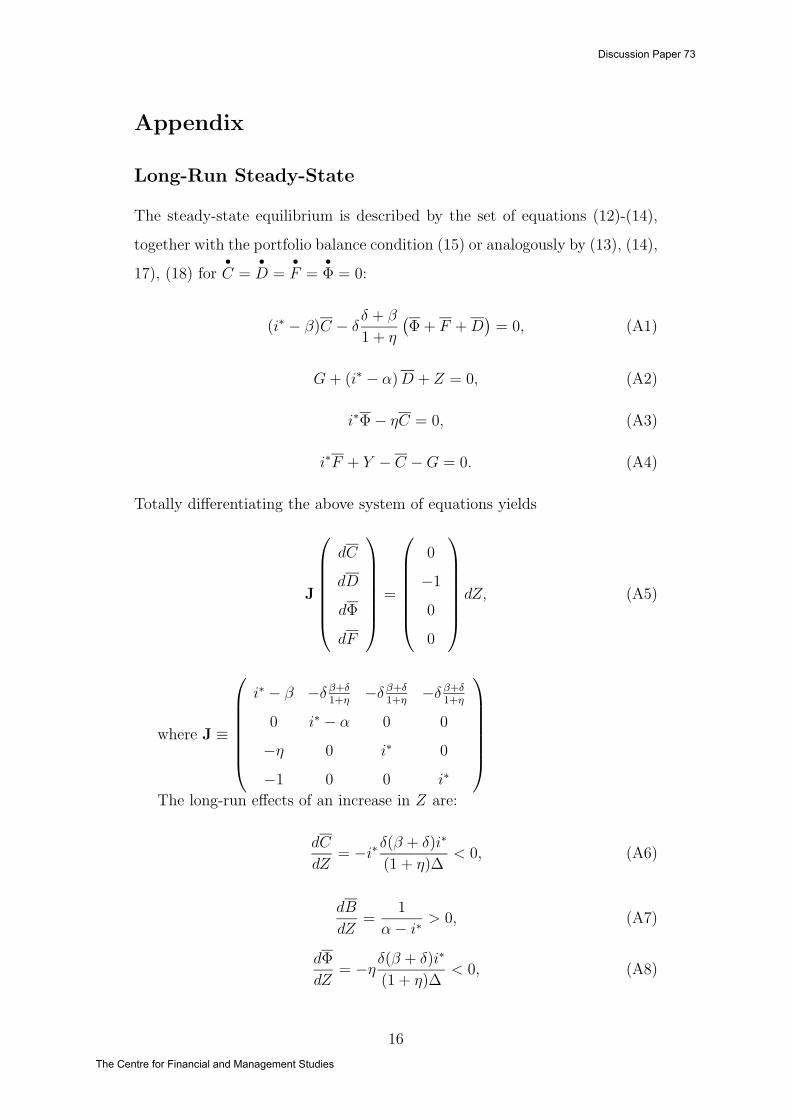
Appendix
Long-Run Steady-State
The steady-state equilibrium is described by the set of equations (12)-(14),
together with the portfolio balance condition (15) or analogously by (13), (14),
17), (18) for•
C =•
D =•
F =•
Φ = 0:
(i∗ − β)C − δδ + β
1 + η
(Φ + F + D
)= 0, (A1)
G + (i∗ − α) D + Z = 0, (A2)
i∗Φ − ηC = 0, (A3)
i∗F + Y − C − G = 0. (A4)
Totally differentiating the above system of equations yields
J
dC
dD
dΦ
dF
=
0
−1
0
0
dZ, (A5)
where J ≡
i∗ − β −δ β+δ
1+η−δ β+δ
1+η−δ β+δ
1+η
0 i∗ − α 0 0
−η 0 i∗ 0
−1 0 0 i∗
The long-run effects of an increase in Z are:
dC
dZ= −i∗
δ(β + δ)i∗
(1 + η)∆< 0, (A6)
dB
dZ=
1
α − i∗> 0, (A7)
dΦ
dZ= −η
δ(β + δ)i∗
(1 + η)∆< 0, (A8)
16
Discussion Paper 73
The Centre for Financial and Management Studies
dF
dZ= −
δ(β + δ)i∗
(1 + η)∆< 0, (A9)
where ∆ ≡ (α − i∗)(β + δ − i∗)(i∗ + δ)i∗ > 0.
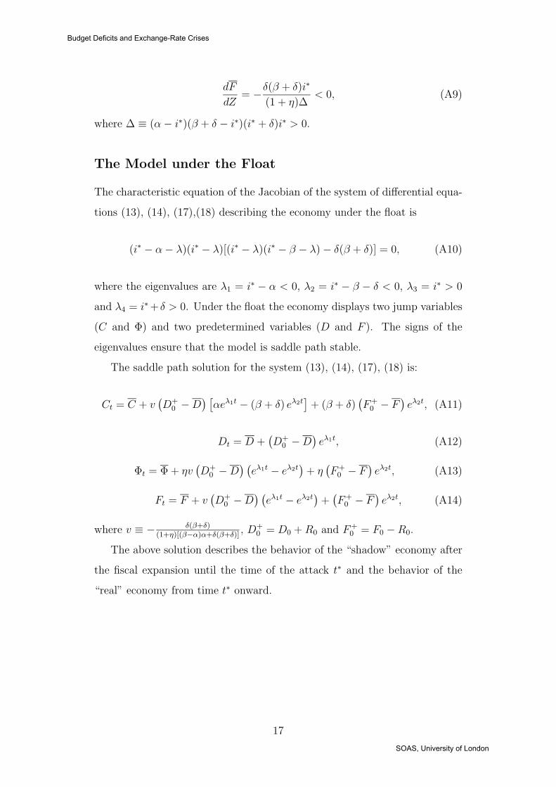
The Model under the Float
The characteristic equation of the Jacobian of the system of differential equa-
tions (13), (14), (17),(18) describing the economy under the float is
(i∗ − α − λ)(i∗ − λ)[(i∗ − λ)(i∗ − β − λ) − δ(β + δ)] = 0, (A10)
where the eigenvalues are λ1 = i∗ − α < 0, λ2 = i∗ − β − δ < 0, λ3 = i∗ > 0
and λ4 = i∗ + δ > 0. Under the float the economy displays two jump variables
(C and Φ) and two predetermined variables (D and F ). The signs of the
eigenvalues ensure that the model is saddle path stable.
The saddle path solution for the system (13), (14), (17), (18) is:
Ct = C + v(D+
0 − D) [
αeλ1t − (β + δ) eλ2t]+ (β + δ)
(F+
0 − F)eλ2t, (A11)
Dt = D +(D+
0 − D)eλ1t, (A12)
Φt = Φ + ηv(D+
0 − D) (
eλ1t − eλ2t)
+ η(F+
0 − F)eλ2t, (A13)
Ft = F + v(D+
0 − D) (
eλ1t − eλ2t)
+(F+
0 − F)eλ2t, (A14)
where v ≡ −δ(β+δ)
(1+η)[(β−α)α+δ(β+δ)], D+
0 = D0 + R0 and F+0 = F0 − R0.
The above solution describes the behavior of the “shadow” economy after
the fiscal expansion until the time of the attack t∗ and the behavior of the
“real” economy from time t∗ onward.
17
Budget Deficits and Exchange-Rate Crises
SOAS, University of London
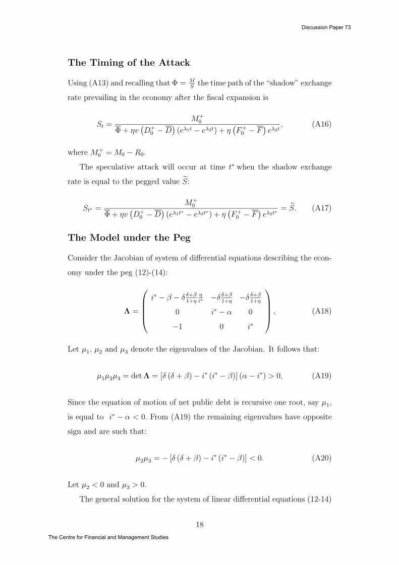
The Timing of the Attack
Using (A13) and recalling that Φ = MS
the time path of the “shadow” exchange
rate prevailing in the economy after the fiscal expansion is
St =M+
0
Φ + ηv(D+
0 − D)(eλ1t − eλ2t) + η
(F+
0 − F)eλ2t
, (A16)
where M+0 = M0 − R0.
The speculative attack will occur at time t∗ when the shadow exchange
rate is equal to the pegged value S:
St∗ =M+
0
Φ + ηv(D+
0 − D)(eλ1t∗ − eλ2t∗) + η
(F+
0 − F)eλ2t∗
= S. (A17)
The Model under the Peg
Consider the Jacobian of system of differential equations describing the econ-
omy under the peg (12)-(14):
Λ =
i∗ − β − δ δ+β
1+η
η
i∗−δ δ+β
1+η−δ δ+β
1+η
0 i∗ − α 0
−1 0 i∗
, (A18)
Let µ1, µ2 and µ3 denote the eigenvalues of the Jacobian. It follows that:
µ1µ2µ3 = detΛ = [δ (δ + β) − i∗ (i∗ − β)] (α − i∗) > 0, (A19)
Since the equation of motion of net public debt is recursive one root, say µ1,
is equal to i∗ − α < 0. From (A19) the remaining eigenvalues have opposite
sign and are such that:
µ2µ3 = − [δ (δ + β) − i∗ (i∗ − β)] < 0. (A20)
Let µ2 < 0 and µ3 > 0.
The general solution for the system of linear differential equations (12-14)
18
Discussion Paper 73
The Centre for Financial and Management Studies
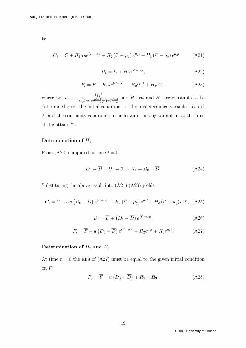
is:
Ct = C + H1αue(i∗−α)t + H2 (i∗ − µ2) eµ2t + H3 (i∗ − µ3) eµ3t, (A21)
Dt = D + H1e(i∗−α)t, (A22)
Ft = F + H1ue(i∗−α)t + H2eµ2t + H3e
µ3t, (A23)
where Let u ≡ −δ β+δ
1+η
α(β−α+δ δ+β1+η
ηi∗ )+δ β+δ
1+η
and H1, H2 and H3 are constants to be
determined given the initial conditions on the predetermined variables, D and
F, and the continuity condition on the forward looking variable C at the time
of the attack t∗.
Determination of H1
From (A22) computed at time t = 0:
D0 = D + H1 = 0 → H1 = D0 − D. (A24)
Substituting the above result into (A21)-(A23) yields:
Ct = C + αu(D0 − D
)e(i∗−α)t + H2 (i∗ − µ2) eµ2t + H3 (i∗ − µ3) eµ3t, (A25)
Dt = D +(D0 − D
)e(i∗−α)t, (A26)
Ft = F + u(D0 − D
)e(i∗−α)t + H2e
µ2t + H3eµ3t. (A27)
Determination of H2 and H3
At time t = 0 the rhs of (A27) must be equal to the given initial condition
on F :
F0 = F + u(D0 − D
)+ H2 + H3. (A28)
19
Budget Deficits and Exchange-Rate Crises
SOAS, University of London
At t = t∗ the rhs of (A25) must be equal to the rhs of (A11) in order to rule
out any discrete jumps of consumption when the fixed regime is abandoned:
αu(D0 − D
)e(i∗−α)t∗ + H2 (i∗ − µ2) eµ2t∗ + H3 (i∗ − µ3) eµ3t∗(A29)
= v(D+
0 − D) [
αeλ1t∗ − (β + δ) eλ2t∗]+ (β + δ)
(F0 − F
)eλ2t∗ .
The constants H2 and H3 can be easily obtained by solving the system of
equations (A28)-(A29).
20
Discussion Paper 73
The Centre for Financial and Management Studies
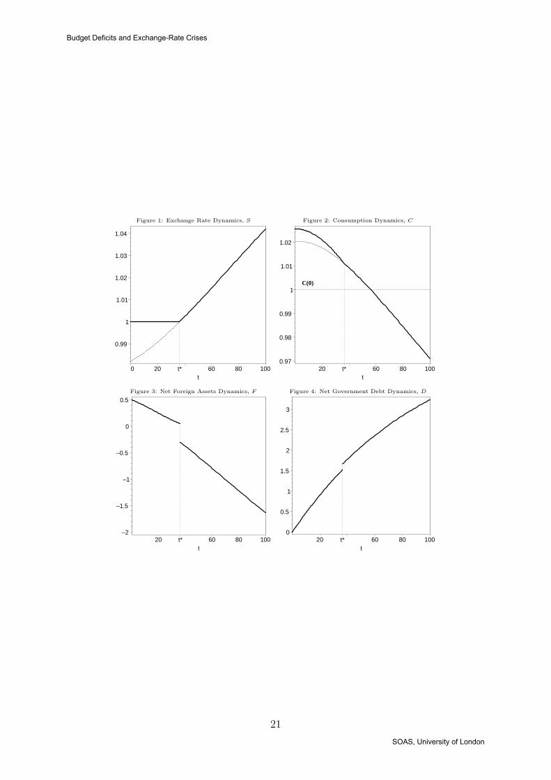
Figure 1: Exchange Rate Dynamics, S Figure 2: Consumption Dynamics, C
0.99
1
1.01
1.02
1.03
1.04
0 20 t* 60 80 100t
C(0)
0.97
0.98
0.99
1
1.01
1.02
20 t* 60 80 100t
Figure 3: Net Foreign Assets Dynamics, F Figure 4: Net Government Debt Dynamics, D
–2
–1.5
–1
–0.5
0
0.5
20 t* 60 80 100t
0
0.5
1
1.5
2
2.5
3
20 t* 60 80 100t
21
Budget Deficits and Exchange-Rate Crises
SOAS, University of London
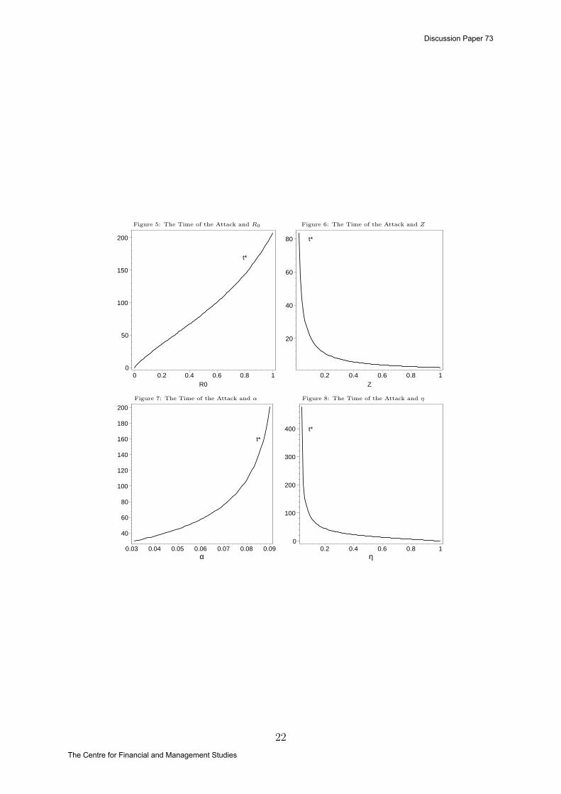
Figure 5: The Time of the Attack and R0 Figure 6: The Time of the Attack and Z
t*
0
50
100
150
200
0 0.2 0.4 0.6 0.8 1R0
t*
20
40
60
80
0.2 0.4 0.6 0.8 1Z
Figure 7: The Time of the Attack and α Figure 8: The Time of the Attack and η
t*
40
60
80
100
120
140
160
180
200
0.03 0.04 0.05 0.06 0.07 0.08 0.09α
t*
0
100
200
300
400
0.2 0.4 0.6 0.8 1η
22
Discussion Paper 73
The Centre for Financial and Management Studies
Recommended