BUREAUCRATIC LIMITS OF FIRM SIZE
Empirical Analysis Using Transaction Cost Economics
A thesis submitted in partial fulfilment of the requirements for the degree of Doctor of Business Administration
by
Staffan Canbäck
Henley Management College Brunel University
February 2002
First prize winner in the EDAMBA (European Doctoral Programmes Association in Management and Business Administration) competi-tion for best European doctoral thesis in 2002.
© 2002 Staffan Canbäck ISBN 0-493-54020-2

ABSTRACT
This thesis tests Oliver Williamson’s proposition that transaction cost economics can explain the limits of firm size. Williamson suggests that diseconomies of scale are manifested through four interrelated factors: atmospheric consequences due to specialisation, bureaucratic insularity, incentive limits of the employment relation and communication distortion due to bounded rationality. Furthermore, Williamson argues that diseconomies of scale are counteracted by economies of scale and can be moderated by adoption of the multidivisional organisation form and by high internal asset specificity. Combined, these influences tend to cancel out and thus there is not a strong, directly observable, relationship between a large firm’s size and performance. A review of the relevant literature, including transaction cost economics, sociological studies of bureaucracy, information-processing perspectives on the firm, agency theory, and studies of incentives and motivation within firms, as well as empirical studies of trends in firm size and industry concentration, corroborates Williamson’s theoretical framework and translates it into five hypotheses: (1) Bureaucratic failure, in the form of atmospheric consequences, bureaucratic insularity, incentive limits and communication distortion, increases with firm size; (2) Large firms exhibit economies of scale; (3) Diseconomies of scale from bureaucratic failure have a negative impact on firm performance; (4) Economies of scale increase the relative profitability of large firms over smaller firms; and (5) Diseconomies of scale are moderated by two transaction cost-related factors: organisation form and asset specificity. The hypotheses were tested by applying structural equation models to primary and secondary cross-sectional data from 784 large US manufacturing firms. The statistical analyses confirm the hypotheses. Thus, diseconomies of scale influence the growth and profitability of firms negatively, while economies of scale and the moderating factors have positive influences. This implies that executives and directors of large firms should pay attention to bureaucratic failure.

To Charlotte, Simon and Rasmus

v
CONTENTS
ABSTRACT .......................................................................................................... iii LIST OF FIGURES ........................................................................................... viii LIST OF TABLES .................................................................................................. x ACKNOWLEDGEMENTS ................................................................................. xii VITAE .................................................................................................................. xiv
1. SUMMARY .................................................................................................. 1
2. INTRODUCTION TO THE RESEARCH ............................................ 10
2.1 RESEARCH OBJECTIVES ............................................................... 13 2.1.1 Problem Definition ............................................................... 13 2.1.2 Importance of the Research ................................................. 18
2.2 DIMENSIONS OF FIRM SIZE ........................................................ 21 2.2.1 Definition of the Firm ........................................................... 21 2.2.2 Definition of Size .................................................................. 23
2.3 TRENDS IN FIRM SIZE ................................................................... 26
3. LITERATURE REVIEW .......................................................................... 31
3.1 THEORETICAL FRAMEWORK .................................................... 31 3.1.1 Reasons for Limits ................................................................ 32 3.1.2 Nature of Limits .................................................................... 34 3.1.3 Economies of Scale ............................................................... 40 3.1.4 Moderating Influences on Firm-Size Limits ..................... 40
3.2 EVIDENCE ........................................................................................ 46 3.2.1 Diseconomies of Scale .......................................................... 47 3.2.2 Economies of Scale ............................................................... 61 3.2.3 Moderating Factors .............................................................. 66 3.2.4 Industry Influence ................................................................ 73 3.2.5 Conclusion ............................................................................. 74
4. THEORETICAL FRAMEWORK AND RESEARCH HYPOTHESES .......................................................................................... 77
5. METHODOLOGY .................................................................................... 83
5.1 APPROACH TO QUANTITATIVE ANALYSIS .......................... 83 5.1.1 Research Philosophy ............................................................ 84 5.1.2 Statistical Technique ............................................................. 86
vi
5.2 DATA OVERVIEW........................................................................... 96 5.2.1 Definitions and Sources ....................................................... 96 5.2.2 Inconsistent Data, Outliers and Effective Sample
Sizes ...................................................................................... 101 5.2.3 Data Transformation, Non-Normality,
Heteroscedasticity and Linearity ...................................... 107
6. RESULTS .................................................................................................. 118
6.1 SUB-MODEL A: RELATIONSHIP BETWEEN FIRM SIZE AND DISECONOMIES OF SCALE AND ECONOMIES OF SCALE .............................................................................................. 123 6.1.1 Diseconomies of Scale ........................................................ 123 6.1.2 Economies of Scale ............................................................. 138
6.2 SUB-MODEL B: RELATIONSHIP BETWEEN DISECONOMIES OF SCALE, ECONOMIES OF SCALE, MODERATING FACTORS AND FIRM PERFORMANCE ...... 144 6.2.1 Diseconomies of Scale and Their Impact on Firm
Performance ......................................................................... 144 6.2.2 Economies of Scale ............................................................. 157 6.2.3 Moderating Factors ............................................................ 162 6.2.4 Complete Sub-Model b ...................................................... 176
6.3 SUMMARY OF FINDINGS FROM STRUCTURAL EQUATION MODELS ................................................................... 190
7. INTERPRETATION AND DISCUSSION ........................................ 193
7.1 SUMMARY OF FINDINGS ........................................................... 194 7.2 LIMITATIONS OF THE RESEARCH .......................................... 208 7.3 FURTHER RESEARCH .................................................................. 210
8. CONCLUSION ....................................................................................... 212
APPENDIX A: LITERATURE REFERENCES PERTAINING TO DISECONOMIES OF SCALE ....................................................................... 217
APPENDIX B: CORRELATION ANALYSES ............................................ 220
DEFINITION OF SIZE ............................................................................ 220 DEFINITION OF FIRM PERFORMANCE ........................................... 223
APPENDIX C: COMPLETE PATH DIAGRAMS, INCLUDING CORRELATIONS ............................................................................................ 227

vii
REFERENCES ................................................................................................... 237
NAME INDEX ................................................................................................... 250
SUBJECT INDEX .............................................................................................. 253

viii
FIGURES
Figure 1. Theoretical Framework and Hypotheses ......................................... 4 Figure 2. Neoclassical Relationship between Unit Cost and Output .......... 15 Figure 3. McConnell/Stigler Relationship between Unit Cost and
Output ...................................................................................................... 16 Figure 4. Production Costs and Transaction Costs as a Function of
Asset Specificity ...................................................................................... 44 Figure 5. Theoretical Framework and Hypotheses ....................................... 81 Figure 6. Histograms for Non-Normal Variables ........................................ 111 Figure 7. Heteroscedasticity and Linearity Analysis ................................... 112 Figure 8. Boxplots for Ordinal Variables ....................................................... 116 Figure 9. Theoretical Framework, Hypotheses and Analytical Models ... 121 Figure 10. Atmospheric Consequences versus Size ..................................... 126 Figure 11. Bureaucratic Insularity versus Size ............................................. 128 Figure 12. Incentive Limits versus Size ......................................................... 130 Figure 13. Communication Distortion versus Size ...................................... 132 Figure 14. Diseconomies of Scale versus Size ............................................... 135 Figure 15. Matrix Representation of Diseconomies of Scale versus Size .. 136 Figure 16. Fixed Cost versus Size: Total Sample .......................................... 140 Figure 17. Fixed Cost versus Size: High Fixed-Cost and
Low Fixed-Cost Sub-Samples ............................................................. 141 Figure 18. Economies of Scale versus Size .................................................... 142 Figure 19. Firm Performance versus Atmospheric Consequences ............ 145 Figure 20. Firm Performance versus Bureaucratic Insularity .................... 147 Figure 21. Firm Performance versus Incentive Limits ................................ 148 Figure 22. Firm Performance versus Communication Distortion ............. 150 Figure 23. Firm Performance versus Diseconomies of Scale:
Not Adjusted for Survivor Bias .......................................................... 152 Figure 24. Firm Performance versus Diseconomies of Scale:
Adjusted for Survivor Bias .................................................................. 155 Figure 25. Firm Performance versus Diseconomies of Scale and
Economies of Scale ............................................................................... 158 Figure 26. M-Form Organisation versus Size ............................................... 165 Figure 27. Firm Performance versus Diseconomies of Scale,
Economies of Scale and M-Form Organisation ................................ 167 Figure 28. Asset Specificity versus Size ......................................................... 172 Figure 29. Firm Performance versus Diseconomies of Scale,
Economies of Scale and Asset Specificity .......................................... 174 Figure 30. Complete Sub-Model b: Includes Diseconomies of Scale,
Economies of Scale and Moderating Factors .................................... 178 Figure 31. Matrix Representation of Complete Sub-Model b ..................... 179 Figure 32. Pruned Sub-Model b ...................................................................... 186

ix
Figure 33. Stylised Cost Curves ...................................................................... 197 Figure 34. Stylised Growth Curves ................................................................ 199 Figure 35. Stylised Partial Performance Curve ............................................ 201 Figure 36. Cost Curve for Current Sample ................................................... 203 Figure 37. Growth Curve for Current Sample .............................................. 204 Figure 38. Partial Performance Curve for Current Sample ........................ 205

x
TABLES
Table 1. Summary of Findings ............................................................................ 8 Table 2. Definition of the Firm and Firm Size ................................................ 25 Table 3. Links between Limiting Factors and Consequences ...................... 39 Table 4. Comparison of Agency Costs and Transaction Costs .................... 54 Table 5. Sources of Limits of Firm Size ............................................................ 61 Table 6. Potential Moderators of Diseconomies of Scale .............................. 73 Table 7. Extended TCE-Based “Limits of Firm Size” Framework ............... 76 Table 8. Select Economic Indicators for the United States ............................ 97 Table 9. Overview of Variables Used in the Analyses .................................. 98 Table 10. Overview of Supporting Variables ................................................ 100 Table 11. Overview of Outliers ....................................................................... 103 Table 12. Multivariate Outliers ....................................................................... 103 Table 13. Effective Sample Sizes for Sub-Model a ........................................ 104 Table 14. Effective Sample Sizes for Sub-Model b ....................................... 104 Table 15. Multivariate Test for Missing Completely at Random
(MCAR) .................................................................................................. 107 Table 16. Overview of Transformation Formulas ........................................ 108 Table 17. Univariate Normality Statistics for Untransformed Variables.. 109 Table 18. Univariate Normality Statistics for Transformed Variables ...... 110 Table 19. Box’s M Test for Heteroscedastic Variables ................................. 115 Table 20. Levene Test for Ordinal Variables ................................................. 117 Table 21. Regression Weight for Atmospheric Consequences versus
Size .......................................................................................................... 126 Table 22. Regression Weights for Bureaucratic Insularity versus Size ..... 128 Table 23. Regression Weights for Incentive Limits versus Size ................. 131 Table 24. Regression Weight for Communication Distortion versus
Size .......................................................................................................... 133 Table 25. Regression Weights for Diseconomies of Scale versus Size ...... 137 Table 26. Regression Weights for Fixed Cost versus Size ........................... 141 Table 27. Regression Weight for Economies of Scale versus Size .............. 143 Table 28. Regression Weights for Firm Performance versus
Atmospheric Consequences ................................................................ 146 Table 29. Regression Weights for Firm Performance versus
Bureaucratic Insularity ......................................................................... 148 Table 30. Regression Weights for Firm Performance versus
Incentive Limits .................................................................................... 149 Table 31. Regression Weights for Firm Performance versus
Communication Distortion ................................................................. 150 Table 32. Regression Weights for Firm Performance versus
Diseconomies of Scale: Not Adjusted for Survivor Bias ................. 153

xi
Table 33. Regression Weights for Firm Performance versus Diseconomies of Scale: Adjusted for Survivor Bias ......................... 156
Table 34. Regression Weights for Firm Performance versus Diseconomies of Scale and Economies of Scale ................................ 160
Table 35. Regression Weights for Firm Performance versus Diseconomies of Scale, Economies of Scale and M-form Organisation ........................................................................... 166
Table 36. Regression Weights for Firm Performance versus Diseconomies of Scale, Economies of Scale and M-Form Organisation .......................................................................... 168
Table 37. Regression Weights for Asset Specificity versus Size ................ 173 Table 38. Regression Weights for Firm Performance versus
Diseconomies, Economies of Scale and Asset Specificity ............... 175 Table 39. Regression Weights for Complete Sub-Model b: Includes
Diseconomies of Scale, Economies of Scale and Moderating Factors .............................................................................. 180
Table 40. Comparison of Parsimony for Competing Models ..................... 184 Table 41. Regression Weights for Pruned Sub-Model b .............................. 187 Table 42. Occurrence of Significant Critical Ratios of Differences
during Random Sample Test .............................................................. 189 Table 43. Summary of Statistical Findings .................................................... 191 Table 44. Summary of Findings ...................................................................... 194

xii
ACKNOWLEDGEMENTS
My wife Charlotte Heyden encouraged me throughout the years of effort.
At dark moments she urged me to continue my research, she supported
my late nights of reading, analysis and writing, and she was my main day-
to-day adviser on theoretical and analytical issues. Without her, this thesis
would never have been written.
My sons Simon and Rasmus Canbäck motivated me by forcing me to be a
scholarly role model. To my pleasant surprise, they have stayed abreast of
my progress. They now aspire to higher education, but probably outside
the realms of business and economics studies.
Throughout the years, my parents Ulla and Owe Canbäck have been
beacons of inspiration. From my childhood and onwards they instilled in
me a respect for learning and the importance of intellectual inquiry.
During the years of research, they often provided logistical assistance.
Professor Phillip Samouel, Dean of Kingston Business School, has
supervised my research superbly, combining insightful feedback with
patience. He based his feedback on an amazingly detailed understanding
of the intricacies of the research. Furthermore, his ability to nudge me
forward at the right time was immensely helpful. Dr David Price,

xiii
Director of Studies of the Doctoral Programmes at Henley Management
College, created a platform for me from which I could pursue this
research, even though the topic did not fit naturally within existing
research themes at Henley.
Finally, I am indebted to Henley Management College, which provided a
stimulating research environment, and to the Marcus Wallenberg
Foundation, which supported the research with a scholarship.

xiv
VITAE
Education
Royal Institute of Technology (Stockholm, Sweden): Master of Science in Engineering, 1975–1979
Harvard Business School (Boston, Massachusetts): Master in Business Administration, 1981–1983
Multinational Business Institute (Tokyo, Japan): Advanced Management Program in Multinational Business, 1986
Henley Management College (Henley-on-Thames, England): Advanced Postgraduate Diploma in Management Consultancy, 1994–1998
Henley Management College/Brunel University (Henley-on-Thames/Uxbridge, England): Doctor of Business Administration, 1994–2002
Work
ABB (Västerås, Sweden): Systems Development Engineer, 1980–1981
McKinsey & Company (Copenhagen, Denmark; Stockholm, Sweden; Gothenburg, Sweden): Associate, 1984–1989; Partner, 1989–1994
Accenture (London, England): Partner, 1996
Monitor Group (Cambridge, Massachusetts): Partner, 1994–
Board Positions
Monitor Group Nordic (Stockholm, Sweden): Chairman, 1997–2000
Kiwicom (Stockholm, Sweden): Chairman, 2000–2001
CircleLending (Cambridge, Massachusetts): Member, 2000–
Distinctions
Fulbright Scholar, 1981
Marcus Wallenberg Foundation for Advanced Education in International Industrial Entrepreneurship: Scholarship, 1994
EDAMBA competition for best European doctoral thesis in business administration and management studies: First prize, 2002
Other
More than 30 business and academic publications
Referee for the Academy of Management

1. SUMMARY
This research tests whether diseconomies of scale influence corporate
performance. It uses Coasian transaction cost economics (Coase 1937) and
Williamson’s thinking on the nature of diseconomies of scale and the
limits of firm size (Williamson 1975, 1985; Riordan and Williamson 1985)
to develop a theoretical framework for describing diseconomies of scale,
economies of scale, and moderating factors. It validates the framework
against the relevant literature and translates it into five hypotheses. The
hypotheses are tested in structural equation models against the 784 largest
firms in the US manufacturing sector in 1998. The findings are consistent
with Williamson’s limits-of-firm-size framework.
Diseconomies of scale are a neglected area of study (see also Chapter 2).
Observers from Knight ([1921] 1964) to Holmström and Tirole (1989) have
pointed out that our understanding of bureaucratic failure is low. The
neglect is to some extent due to a disbelief in the existence of diseconomies
of scale (e.g., Florence 1933, 12; Bain 1968, 176). It is also due to a dearth of
theoretical frameworks that can help inform our understanding of the
nature of diseconomies of scale. However, if diseconomies of scale did not
exist, then we would presumably see much larger firms than we do today
(Panzar 1989, 38). No business organisation in the United States has more

2
than one million employees1 or more than ten hierarchical levels. No firm
has ever been able successfully to compete in multiple markets with a
diverse product range for an extended period of time. Common sense tells
us that there are limits to firm size. Common sense does not, however,
prove the point. Unfortunately, scientific inquiry has not yet focused on
finding such proof.
The US manufacturing sector has, as a whole, been remarkably stable over
the last century. Contrary to popular opinion, markets have on average
not become more concentrated (e.g., Nutter 1951; Scherer and Ross 1990).
Large firms are not increasingly dominant. Large manufacturing firms in
the United States employed 16 million people in 1979 versus 11 million in
1994, while private sector employment grew from 99 to 123 million people
(Council of Economic Advisers 1998; Fortune 1995a).
Williamson (1975, 117–131) found that the limits of firm size are
bureaucratic in origin and can be explained by transaction cost economics
(see also Chapter 3). He identified four main categories of diseconomies of
scale: atmospheric consequences due to specialisation, bureaucratic insularity,
incentive limits of the employment relation and communication distortion
1 The largest company, Wal-Mart Stores, Inc., had 910,000 employees in 1998. The largest
manufacturing company, General Motors Corporation, had 594,000 employees.

3
due to bounded rationality. Economies of scale2 in production costs and
transaction costs tend to offset these diseconomies of scale (Riordan and
Williamson 1985). Moreover, the disadvantages of bureaucracy can be
moderated by using the multidivisional organisation form (M-form) and by a
judicious optimisation of the degree of integration through high internal
asset specificity (Williamson 1975, 1985). Together, these influences on firm
performance form the theoretical framework used in this research.
The literature review supported the framework. There are, as far as this
researcher could determine, around 60 pieces of work that deal with
diseconomies of scale in a substantial manner (see Appendix A). Based on
these and other more fragmentary sources, it was possible to validate
Williamson’s framework and his categorisation of the factors driving
diseconomies of scale, economies of scale and the moderating factors,
except that the literature review was inconclusive regarding economies of
scale. The framework was translated into five testable hypotheses,
summarised in Figure 1 (see also Chapter 4).
2 A standard definition of economies of scale, taken from The New Palgrave: A Dictionary of
Economics, is that they exist if the unit cost of producing one additional unit of output decreases. They are driven by (a) the existence of indivisible inputs, (b) set-up costs and (c) the benefits of division of labour (Eatwell, Milgate and Newman 1987, 80–81). In the case of the multi-product firm, economies of scale exist if the ray average cost decreases as output increases.

4
Figure 1. Theoretical Framework and Hypotheses
FirmPerformance
GrowthProfitability
ModeratorsAsset Specificity
M-Form Organisation
Economies of Scale
Diseconomies of ScaleAtmospheric Consequences
Bureaucratic InsularityIncentive Limits
Communication Distortion
Size
THEORETICAL FRAMEWORK AND HYPOTHESES
H1
H2
H3
H4
H5
FirmPerformance
GrowthProfitability
ModeratorsAsset Specificity
M-Form Organisation
Economies of Scale
Diseconomies of ScaleAtmospheric Consequences
Bureaucratic InsularityIncentive Limits
Communication Distortion
SizeSize
THEORETICAL FRAMEWORK AND HYPOTHESES
H1
H2
H3
H4
H5
The first two hypotheses test the tautological statement that diseconomies
of scale and economies of scale increase with firm size. The last three
hypotheses test how a firm’s performance is affected by the diseconomies
of scale, economies of scale and moderating influences.
H1: Bureaucratic failure, in the form of atmospheric consequences,
bureaucratic insularity, incentive limits and communication
distortion, increases with firm size
5
H2: Large firms exhibit economies of scale
H3: Diseconomies of scale from bureaucratic failure have a negative
impact on firm performance
H4: Economies of scale increase the relative profitability of large firms
over smaller firms
H5: Diseconomies of scale are moderated by two transaction cost-
related factors: organisation form and asset specificity
The third hypothesis has four sub-hypotheses, which test each of the
diseconomies of scale factors.
H3a: Atmospheric consequences have a negative impact on the
performance of large firms
H3b: Bureaucratic insularity has a negative impact on the performance of
large firms
H3c: Incentive limits have a negative impact on the performance of large
firms

6
H3d: Communication distortion has a negative impact on the
performance of large firms
The fifth hypothesis has two sub-hypotheses for organisation form and
asset specificity, respectively.
H5a: Large M-form firms perform better than large U-form firms
H5b: High internal asset specificity affects a firm’s performance
positively
The hypotheses were tested against a sample of the 784 largest
manufacturing firms in the United States in 1998, for which primary and
secondary data were collected from a number of sources, including
company organisation charts, official filings and annual reports,
biographies of executives, historical company documents, corporate web
sites, magazine articles, corporate watchdogs, Compustat and academic
research. The hypotheses were operationalised based on the literature
review and it proved possible to collect enough data for most of the
variables to create a statistically robust sample (see also Chapter 5).
Structural equation modelling (SEM) was used to create path diagrams
representing the hypotheses. Two sub-models containing these path
diagrams capture the relationships (see also Chapter 6): sub-model a: firm

7
size and the diseconomies/economies of scale (H1 and H2); and sub-
model b: diseconomies/economies of scale, moderating influences and
firm performance (H3, H4 and H5).
Table 1 summarises the findings for each hypothesis (see also Chapter 7).
All hypotheses were confirmed except for H3d (communication distortion),
for which the result was inconclusive. The strongest negative influence
from diseconomies of scale on a large firm’s performance appears to be on
its ability to grow, while there is less negative influence on profitability.
Thus, Penrose’s claim ([1959] 1995, 261–263) that diseconomies of scale
reduce the growth capability of large firms, appears to be validated.

8
Table 1. Summary of Findings
SUMMARY OF FINDINGSa
Hypothesis Literature Finding Statistical Finding H1: Bureaucratic failure, in the form of atmospheric consequences, bureaucratic insularity, incentive limits and communication distortion, increases with firm size
Confirmed Confirmed
H2: Large firms exhibit economies of scale Confirmed Confirmed H3: Diseconomies of scale from bureaucratic failure have a negative impact on firm performance
Confirmed Confirmed
H3a: Atmospheric consequences have a negative impact on the performance of large firms
Confirmed Confirmed
H3b: Bureaucratic insularity has a negative impact on the performance of large firms
Confirmed Confirmed
H3c: Incentive limits have a negative impact on the performance of large firms
Confirmed Confirmed
H3d: Communication distortion has a negative impact on the performance of large firms
Confirmed Inconclusive
H4: Economies of scale increase the relative profitability of large firms over smaller firms
Inconclusive Confirmed
H5: Diseconomies of scale are moderated by two transaction cost-related factors: organisation form and asset specificity
Confirmed Confirmed
H5a: Large M-form firms perform better than large U-form firms
Confirmed Confirmed
H5b: High internal asset specificity affects a firm’s performance positively
Confirmed Confirmed
a For simplicity, the word ”confirmed” is used, although ”not rejected” is more accurate.
The implications are that diseconomies of scale are real and important
contributors to a firm’s performance, in a negative way. However,
economies of scale can offset some of these negative consequences. Finally,
the use of M-form organisation and pursuit of high internal asset
specificity can moderate the negative impact of diseconomies of scale.
These findings make it possible to create conceptual cost curves and
growth curves that extend neoclassical theory. The curves are found in

9
Chapter 7, together with cost and growth curves plotting data from the
sample used in the research.
There are several practical implications (see also Chapter 8). Among them
are that corporate strategies are interconnected with the organisational
choices made. That is, structure does not necessarily follow strategy. In
light of this, it is understandable that mergers or acquisitions often fail,
especially when the rationale for the merger-and-acquisition activity is to
capture revenue growth opportunities. It is also evident that the focus on
corporate governance over the last decade has its benefits. Other things
equal, good governance allows large corporations to expand their limits-
of-firm-size horizon. Moreover, as initiatives in large corporations are
increasingly team-oriented, it is not surprising that senior executives pay
more attention to motivation and how to structure incentives to extract
optimal effort from the employees.
In the next chapter, the research objectives are defined and the importance
of the research is discussed, linking it back to perspectives on economies of
scale and diseconomies of scale in neoclassical theory and transaction cost
economics. The chapter then explores the definition of the firm and
metrics for measuring firm size. Finally, trends in firm size and
concentration in the US manufacturing sector are discussed.

10
2. INTRODUCTION TO THE RESEARCH
Why are large firms so small? What stops firms from effortlessly
expanding into new businesses? Only fragmentary research exists today as
to why the largest business organisations do not have ten, twenty or a
hundred million employees rather than a few hundred thousand.
According to Arrow (1974, 55) a “tendency to increasing costs with scale of
operation” due to the cost of handling information and the irreversible
cost of building organisational knowledge leads to limits of firm size.
Coase (1937, 397) found that these costs—labelled “diseconomies of scale”
in this thesis to contrast them with “economies of scale”—are associated
with the resources required to manage the firm’s internal planning
processes, as well as the cost of mistakes and the resulting misallocation of
resources, especially under conditions of uncertainty.
The thesis builds on original research carried out in the subject area.
Specifically, it tests whether Williamson’s “limits of firm size” discussion
in Markets and Hierarchies: Analysis and Antitrust Implications (1975, 117–
131) and in The Economic Institutions of Capitalism (1985, 131–162), which
extend Arrow’s and Coase’s arguments, are valid. The findings include a
look at the nature of diseconomies of scale and factors which moderate

11
their impact, as well as a quantification of the impact of diseconomies of
scale on firm performance.
Transaction cost economics (TCE) provides the theoretical foundation for
this research. There are other partial explanations of diseconomies of scale,
such as those found in neoclassical economics (e.g., Mas-Colell, Whinston
and Green 1995; Scherer and Ross 1990); agency theory (e.g., Pratt and
Zeckhauser 1985; Jensen and Meckling 1976); growth theory (e.g., Penrose
[1959] 1995); evolutionary theory (e.g., Nelson and Winter 1982); sociology
(e.g., Blau and Meyer 1987); and Marxist theory (e.g., Marglin 1974). These
explanations are not the focus here, although they will be used to
illuminate and test particular aspects of the TCE argument described in
Chapter 3.
The purpose of the research is to create a theoretically robust and
empirically tested framework that can be used by executives and others to
inform strategic and organisational choices for large corporations. These
choices may help decision-makers achieve higher growth and profitability
by minimising diseconomies of scale due to atmospheric consequences,
bureaucratic insularity, incentive limits and communication distortion (as
defined in Section 3.1.2); to capture economies of scale; to optimise
organisational structures; and to maximise asset specificity within the
corporation.

12
These issues are addressed empirically through a statistical analysis of the
784 largest manufacturing firms in the United States in 1998.3 This limited
analysis4—covering one year, one industry sector and one country—lends
credence to Williamson’s limits-of-firm-size argument; no aspect of his
theoretical discussion is refuted. The analysis also supports Penrose’s
assertion ([1959] 1995, 261–263) that diseconomies of scale mainly reduce
growth of large firms rather than decrease their profitability.
The remainder of this chapter describes the research objectives and their
importance in more detail, defines firm size, and documents trends in firm
size over the last century.
3 Having more than $500 million in annual revenue. 4 The United States was chosen because it is a large and competitive market, the manufacturing
sector was chosen because of the depth of earlier research and the availability of data, and a single, recent, year was chosen because much of the data was not available further back.

13
2.1 RESEARCH OBJECTIVES
This section gives an initial problem definition and discusses the
importance of the research. It spells out why diseconomies of scale are real
and pervasive, yet poorly understood. In fact, while the economics
literature often includes cost curves that bend upward at large firm sizes,
there are only around 60 pieces of work that explicitly discuss the nature
of the diseconomies,5 and only a few of these have attempted to quantify
the diseconomies of scale.
2.1.1 Problem Definition
In the early 1920s, Knight ([1921] 1964, 286–287) observed that “the
diminishing returns to management is a subject often referred to in
economic literature, but in regard to which there is a dearth of scientific
discussion”. Since then, many authorities have referred to the existence of
diseconomies of scale, but no systematic studies of the general issue exist.
The basic dilemma is illustrated by the mismatch between theoretical
expectations and real-world observations. On the one hand, if
diseconomies of scale do not exist, then there should be no limits to firm
growth and size. We would observe an inexorable concentration of
industries and economies until only one global firm was left. The answer
5 There is also a vast literature on the size-distribution of firms, but it generally does not discuss
the specific mechanisms underlying bureaucratic failure.

14
to Coase’s question (1937, 394): “Why is not all production carried on by
one big firm?” would be: it will. Similarly, Stigler (1974, 8) wrote that “if
size were a great advantage, the smaller companies would soon lose the
unequal race and disappear”. This is not happening. On the other hand, if
a given industry has an optimum firm size, then we would expect
increased fragmentation as the overall economy grows. This would be in
line with Stigler’s survivor-principle argument which holds that “the
competition between different sizes of firms sifts out the more efficient
enterprises” (1958, 55). Again, this is not happening. Lucas (1978, 509)
observed that “most changes in product demand are met by changes in
firm size, not by entry or exit of firms”. The size distribution of firms has
been remarkably stable over time for most for the last century, when
measured by number of employees or as a share of the total economy (as
discussed in Section 2.3).
Cost curves (Figure 2) are used in neoclassical theory to illustrate
economies and diseconomies of scale (e.g., Marshall [1920] 1997, 278–292;
Scherer and Ross 1990, 101).

15
Figure 2. Neoclassical Relationship between Unit Cost and Output
NEOCLASSICAL RELATIONSHIP BETWEEN UNIT COST AND OUTPUT
Output (Q)
Long-RunAverage
Cost(AC)
M
Source: Scherer and Ross (1990)
NEOCLASSICAL RELATIONSHIP BETWEEN UNIT COST AND OUTPUT
Output (Q)
Long-RunAverage
Cost(AC)
M
Source: Scherer and Ross (1990)
Output (Q)
Long-RunAverage
Cost(AC)
M
Source: Scherer and Ross (1990)
As the output Q increases, the average cost decreases due to economies of
scale. At a certain point (M) the economies of scale are exhausted, while
diseconomies of scale, presumably driven by diminishing returns to
management (e.g., Coase 1937, 395), start to influence the unit cost. As
output increases, the unit cost increases. In a competitive market, this
implies an equilibrium output M where marginal cost not only equals
marginal revenue, but also intersects long-run average cost at its
minimum (e.g., Mankiw 1998, 296).
In reality, however, this is not what is observed. Rather, the cost-
minimising part of the curve covers a wide range of outputs, and only at
high output levels do diseconomies set in, if ever (Panzar 1989, 37–38).

16
McConnell’s quantification (1945, 6) and Stigler’s illustration (1958, 59),
reproduced in Figure 3, are typical.
Figure 3. McConnell/Stigler Relationship between Unit Cost and Output
MCCONNELL/STIGLER RELATIONSHIP BETWEEN UNIT COST AND OUTPUT
Output (Q)
Long-RunAverage
Cost(AC)
Source: McConnell (1945), Stigler (1958)
1M 2M
MCCONNELL/STIGLER RELATIONSHIP BETWEEN UNIT COST AND OUTPUT
Output (Q)
Long-RunAverage
Cost(AC)
Source: McConnell (1945), Stigler (1958)
1M 2M
Output (Q)
Long-RunAverage
Cost(AC)
Source: McConnell (1945), Stigler (1958)
1M 2M
This shape of the cost curve reconciles several real-world observations.
(1) It explains why large and small firms can coexist in the same industry.
There is a wide range of outputs, between the points 1M and 2M , for
which the unit cost is more or less constant. (2) It is consistent with Lucas’s
observation (1978, 509) that, as the economy grows, existing firms tend to
expand supply to meet additional demand, because most firms operate
with outputs Q below the 2M inflexion point. (3) It eliminates the
supposition that economies of scale are exhausted at approximately the
same point that diseconomies of scale start increasing unit cost, which is

17
indicated with 1M being much to the left of 2M . (4) It demonstrates that
there are indeed limits to firm size due to diseconomies of scale, as shown
by the increasing unit cost beyond 2M —large firms have not expanded
indefinitely.
However, if the reasoning above is correct, it is still unclear why the cost
curve bends upwards at 2M . Neoclassical theory does not provide a
satisfactory answer. As Simon ([1947] 1976, 292) said: “the central problem
is not how to organize to produce efficiently (although this will always
remain an important consideration), but how to organize to make
decisions”.6 The first part of this statement refers to the negative derivative
of the cost curve at outputs smaller than 1M , where economies of scale in
production have not yet been exhausted, while the second part applies to
the upward slope, where diseconomies of scale due to diminishing returns
to management set in beyond 2M .
Clarifying “how to organise to make decisions”—and thus the upward
bend of the cost curve—will help executives optimise corporate
performance. The current research investigates whether transaction cost
economics can more thoroughly explain diseconomies of scale and what
drives these diseconomies. It picks up on a debate that harks back to the 6 Simon echoed the writing of Robertson (1923, 25): ”It is the economies of large-scale government
rather than of large-scale technique which dictate the size of the modern business unit”. (Note: government here refers to corporate organisation and governance, not national government.)

18
early 1930s when Florence (1933) and Robinson (1934), respectively,
argued the case against and for limits of firm size. Florence believed that
optimum firm size meant maximum firm size: “the more the amount of
any commodity provided the greater the efficiency” and “there is in my
view no theoretical limit to the increase in the physical return obtainable
by larger-scale operations” (p. 12). He argued that no organisation would
be too large for a single leader to control and thought that the only reason
this had not happened yet was a certain lag between what managers at the
time assumed they could do and the inevitable outcome (p. 47).
In contrast, Robinson did not subscribe to this reasoning and he believed
strongly in “the increasing costs of coordination required for the
management of larger units” (p. 242). He argued that the existing facts—
the then newly released first report on the size distribution of British
firms—supported the notion that optimum firm size was less than
maximum firm size (p. 256).
2.1.2 Importance of the Research
Diseconomies of scale have not been extensively studied and thus there
may be a genuine gap in our understanding of the firm. Transaction cost
economics may help fill this gap because the theory embeds a number of
concepts relating to the limits of the firm. Filling the gap may not only

19
affect the way we think about strategy and structure, but also help
executives make more effective decisions.
Limits-of-firm-size is not a major field of study (Coase 1993a, 228;
Holmström and Tirole 1989, 126). There are around 60 articles or books
that deal with the topic in a meaningful way (see Chapter 3 for a review
and Appendix A for a list of references). Williamson (1985, 153), for
example, stated that our understanding of bureaucratic failure is low
compared with what we know of market failure. Given the relative
slowdown in the growth of large firms over the last 30 years (see
Section 2.3), understanding why market-based transactions are slowly
winning over internally-based transactions matters more than ever.
The second reason why this research is academically important is that it
uses transaction cost economics in a somewhat new fashion. The 1970s
were the defining years of TCE. At that time, large firms still appeared set
to become ever more dominant, and TCE reflects this Zeitgeist. Thus, many
of the theory’s applications have been in antitrust cases, rather than in
studies of internal organisation. Further, TCE has arguably evolved over
time from a general theory for understanding industrial organisation to a
tool for primarily analysing vertical integration. For example, Shelanski
and Klein (1995) surveyed the empirical transaction-cost-economics
literature; out of 118 journal articles published between 1976 and 1994,

20
87 (74 per cent) related to vertical integration, make/buy decisions, or
hybrid forms of vertical integration.7 Williamson’s introductory overview
of TCE in the Handbook of Industrial Organization (1989, 150) called vertical
integration the paradigm problem of TCE. This research breaks with that
tradition by looking at the firm as a whole, rather than its vertical
integration characteristics.
Limits of firm size are also a real and difficult problem for business
executives. The cost of suboptimal size—that is, a firm that is too large—is
probably significant. For example, up to 25 per cent (Riahi-Belkaoui
1994, 35–64) of the cost of goods sold of a large manufacturing firm can be
attributed to organisational slack, often embedded in communication
problems, bureaucratic inefficiencies and other diseconomies of scale
discussed in detail in Chapter 3. Moreover, large firms have a tendency
slowly to decline and disappear (Hannah 1996, 1). Shedding light on why
this is the case may be socially and privately beneficial, Hannah pointed
out, because “we have made great strides in storytelling, but a clearer,
surer recipe for sustained success for large corporations has remained
elusive” (p. 24).
7 Shelanski and Klein claimed that vertical integration research has declined as a share of the total
over time, but a categorisation by year shows that the share is stable or may in fact have increased. 1976–1979: 5 articles, 40 per cent vertical integration; 1980–1984: 26 articles; 73 per cent vertical integration; 1985–1989: 53 articles, 72 per cent vertical integration; 1990–1994: 34 articles, 82 per cent vertical integration.

21
2.2 DIMENSIONS OF FIRM SIZE
This section defines size and shows the trends in firm size in the US
manufacturing sector. Large manufacturing firms in the US have shrunk
relative to the total manufacturing sector and the economy as whole over
the last 20 to 25 years, while overall industry concentration has been rather
stable over the last 100 years. Applying the survivor principle (see p. 14,
above), this implies that there are indeed limits to firm size.
2.2.1 Definition of the Firm
To begin with, there are a number of definitions of what a firm is. The first,
based on Coase (1937, 389), Penrose ([1959] 1995, 15), and Arrow
(1964, 403; 1974, 33) holds that the boundary of the firm is where the
internal planning mechanism is superseded by the price mechanism. That
is, the firm’s border is at the point where transactions are regulated by the
market rather than by administration. In most cases this means that the
operating firm is equivalent to the legal corporation. An important, if rare,
exception is a corporation in which divisions are totally self-contained
profit centres. In this case the parent company is not a firm, because the
company’s divisions by definition trade between themselves through
market-based transfer prices.

22
The second definition is that ownership sets a firm’s boundaries (e.g., Hart
1995, 5–8). With this definition, a firm is the combination of activities for
which the bearers of residual risk are one and the same. One problem with
this definition is that employees are not “owned”, so they therefore would
not be considered part of the firm. Another issue is how units such as a
partly-owned subsidiary should be treated. For example, General Motors
Corporation owned 82 per cent of Delphi Automotive Systems in early
1999, but Delphi would not be viewed as part of General Motors under the
above definition. Still, this definition is quite similar to Coase’s because
employment contracts can be viewed as temporary ownership claims, and
partial ownership is still uncommon even though alliances and carve-outs
have grown in popularity.
A third definition sees the firm as a network (Richardson 1972, 884–887).
McDonald’s Corporation, for example, extends far beyond its corporate
ownership, because it also consists of a network of thousands of
franchisees over whom McDonald’s have a high degree of contractual
control (Rubin 1990, 134–144).8
The fourth definition is based on the firm’s sphere of influence. This
includes distributors, alliance partners, first- and second-tier suppliers,
8 18,265 at the end of 1999.

23
and so on (Williamson 1985, 120–122). Toyota Motor Corporation, for
example, directly employed 215,000 people in 2000, but its sphere of
influence probably extended over more than one million people.
In all four cases, it is theoretically somewhat difficult to draw the
boundaries of the firm and to distinguish the firm from the whole
economy. Nevertheless, it is, to use the words of Kumar, Rajan and
Zingales (1999, 10), possible to create an “empirical definition”. For the
purposes of this thesis, the firm is defined as having commonly owned
assets—the ownership definition—but employees are also treated as part
of the firm. This definition relates closely to Hart’s definition (1995, 7), and
publicly available data follow it. It is also commonly used in research
(Kumar, Rajan and Zingales 1999, 11). Thus, a firm is an incorporated
company (the legal entity) henceforth.
2.2.2 Definition of Size
There are various ways to measure the size of a firm. Size is most often
defined as annual revenue, especially by the business press. However, this
measure is basically meaningless because it tells nothing about the depth
of the underlying activity. Based on this measure, the world’s four largest
companies were Japanese trading houses in 1994 (Fortune 1995b). They

24
had between 7,000 and 80,000 employees, but almost no vertical
integration.
A better measure of size is value added, which is more or less equivalent
to revenue less externally purchased products and services. This metric
gives a precise measure of activity, but it is usually not publicly available
for individual firms.
Number of employees is the most widely used measure of size. A review
by Kimberley claims that more than 80 per cent of academic studies use
this measure (1976, 587). In line with Child’s observation (1973, 170) that
“it is people who are organized”, it is not surprising that the number of
employees is the most used metric for measuring firm size.
Finally, assets can define size (e.g., as described by Grossman and Hart
1986, 693–694). As with revenue, this measure may not reflect underlying
activity; but for manufacturing firms, asset-to-value-added ratios are fairly
homogeneous. Asset data for individual firms are usually available back to
the 1890s and are therefore a practical measure in longitudinal studies.
In sum, the best measures of size are value added and number of
employees, although assets can be used in certain types of studies. This
research uses number of employees as the size metric because the data are

25
available and diseconomies of scale should be associated with human
frailties. Moreover, this research deals with bureaucratic failure, which in
the end is the result of coordination costs. Such costs are best measured in
relation to number of employees (Kumar, Rajan and Zingales 1999, 12).
The definitions are summarised in Table 2 with the suitability for the
research at hand indicated by the shadings, ranging from high (black) to
low (white).
Table 2. Definition of the Firm and Firm Size
DEFINITION OF THE FIRM AND FIRM SIZE
Size Metric
Firm Definition Internal Planning
(Coase)
Ownership
Network Sphere of Influence
Revenue Value Added Employees Assets

26
2.3 TRENDS IN FIRM SIZE
The US economy is the basis for the analysis in the current research
because it is large, fairly homogenous and transparent, and it has a high
level of competition between firms. Within this economy, the research
focuses on the manufacturing sector.9
Large manufacturing firms play a major role in the US economy. The
Fortune industrial 500 companies controlled more than 50 per cent of
corporate manufacturing assets and employed more than eleven million
people in 1994, the last year for which the Fortune industrial ranking was
compiled (Fortune 1995a). Their sphere of influence was approximately 40
million employees out of a total private sector workforce of 123 million.
Contrary to popular belief, however, the importance of large firms is not
increasing and has not done so for many years. Studies show that large
manufacturing firms are holding steady as a share of value added since
circa 1965 (Scherer and Ross 1990, 62). Their share of employment in the
manufacturing sector has declined from around 60 per cent (1979) to
around 50 per cent (1994). Moreover, as a share of the total US economy,
they are in sharp decline. Large manufacturing firms employed 16 million
people in 1979 versus 11 million in 1994 (Fortune 1995a, 185), while private
9 Alternative approaches would be to study the global manufacturing sector, the total US private
sector, or both. However, statistics on the global manufacturing sector are not reliable, and the non-manufacturing sectors are often highly regulated.

27
sector employment grew from 99 to 123 million people (Council of
Economic Advisers 1998, 322) over the same time period.
Further evidence that large firms do not increasingly dominate the
economy is available from a number of historical studies. Aggregate
industry concentration has changed little since the early part of the last
century.10 Nutter (1951) studied the concentration trend between 1899 and
1939 and found no signs of increased aggregate concentration during this
period, mainly because new, fragmented industries emerged, while older
ones consolidated (pp. 21, 33). Bain (1968) found the same trend between
1931 and 1963, but with less variability between industries. Scherer and
Ross (1990, 84) used Nutter’s method and showed that aggregate
concentration increased slightly, from 35 per cent in 1947 to 37 per cent in
1982. Similarly, Mueller and Hamm (1974, 512) found an increase in four-
firm concentration from 40.5 per cent to 42.6 per cent between 1947 and
1970, with most (70 per cent) of the increase between 1947 and 1963.
Bain (1968, 87) calculated that the assets controlled by the largest 200
nonfinancial firms amounted to about 57 per cent of total nonfinancial
assets in 1933.11 He also estimated that the 300 largest nonfinancial firms
10 Note that there have been significant changes within individual industries. 11 A similar study by Berle and Means ([1932] 1991) has been partly discredited. For example,
Scherer and Ross (1990, 60) found that Berle and Means, based on the “meager data then available,...overestimated the relative growth of the largest enterprises”.

28
accounted for 55 per cent of nonfinancial assets in 1962. The largest 200
firms therefore accounted for approximately 50 per cent of nonfinancial
assets in 1962 (using the current researcher’s estimate of the assets
controlled by the 100 smallest firms in the sample). This researcher’s data
showed that the top 200 nonfinancial firms controlled less than 50 per cent
of the total nonfinancial assets in 1994. Adelman (1978) observed a similar
pattern when he studied the 117 largest manufacturing firms between 1931
and 1960. He found that concentration was the same at the beginning and
at the end of the period (45 per cent). He concluded that “overall
concentration in the largest manufacturing firms has remained quite stable
over a period of 30 years, from 1931 to 1960”. Allen (1976) updated
Adelman’s number to 1972 and reached the same conclusion. The current
research replicated the analysis for 1994 and found the same concentration
number to be 45 per cent. Both sets of longitudinal data indicate that large
firms represent a stable or declining fraction of the manufacturing sector.
Finally, Bock (1978, 83) studied the share of value added contributed by
the largest manufacturing firms between 1947 and 1972. There was a large
increase between 1947 and 1954, and a further slight increase until 1963.
Between 1963 and 1972, there was no increase. Scherer and Ross (1990, 62)
confirmed the lack of increase through the end of the 1980s. Sutton

29
(1997, 54–55) reached a similar conclusion in a comparison of
concentration in the US manufacturing sector between 1967 and 1987.
As for the future, the stock market does not expect the largest firms to
outperform smaller firms. The stock market valuation of the largest firms,
relative to smaller firms, has declined sharply between 1964 and 1998
(Farrell 1998). In 1964 the largest 20 firms comprised 44 per cent of total
stock market capitalisation in the United States; in 1998 they accounted for
19.5 per cent. Market value primarily reflects future growth and profit
expectations, and thus the market is increasingly sceptical of large firms’
ability to compete with smaller firms. This could be due to industrial
evolution, but if it is assumed that diseconomies of scale do not exist, then
the largest 20 firms should presumably be able to compensate for a relative
decline in their mature businesses by effortlessly growing new businesses.
A study of firms on the New York stock exchange (Ibbotson Associates
1999, 127–143) similarly showed that small firms outperformed large firms
between 1926 and 1998. The total annual shareholder return over the
period was 12.1 per cent for the largest size decile and 13.7 per cent for the
second largest size decile. It increased steadily to 21.0 per cent for the
smallest size decile (p. 129). The real return to shareholders after
adjustment for risk (using the capital asset pricing model) was �0.28 per
cent for decile 1, +0.18 per cent for decile 2 and rising steadily to +4.35 per

30
cent for decile 10 (p. 140). Note, however, that market capitalisation was
used as the definition of size in this study.
The above evidence shows that concentration in the manufacturing
sector—defined as the share of value added, employment, assets or market
capitalisation held by large firms—has changed little or has declined over
much of the last century. The size of large manufacturing firms has kept
pace with the overall growth of the manufacturing part of the economy
since the 1960s in value-added terms, but has declined in employment
terms since 1979 (and has declined relative to the total US corporate sector
and the global corporate sector). This indicates that there is a limit to firm
size and that this limit may be decreasing in absolute terms, all of which
supports the research findings of this thesis.
The next chapter explores these limits of firm size through a review of the
relevant literature. A theoretical framework is constructed based on
transaction cost economics, and the literature is surveyed to validate the
framework.

31
3. LITERATURE REVIEW
The literature review is divided into two parts. The first part defines the
theoretical framework and discusses the transaction-cost-economics
literature relating to the framework. The second part examines the
evidence in transaction cost economics and other fields which supports
(and occasionally contradicts) the theoretical framework. The chapter
shows that a robust theoretical framework can be constructed based on
transaction cost economics, and that the theoretical and empirical
literature is congruent with this framework.
3.1 THEORETICAL FRAMEWORK
Transaction cost economics focuses on the boundary of the firm
(Holmström and Roberts 1998, 73; Williamson 1981, 548)—that is, the
distinction between what is made internally in the firm and what is
bought and sold in the marketplace. The boundary can shift over time and
for a number of reasons, and the current research looks at one aspect of
these shifts. As firms internalise transactions, growing larger, bureaucratic
diseconomies of scale appear. Thus, a firm will reach a size at which the
benefit from the last internalised transaction is offset by bureaucratic
failure. Two factors moderate these diseconomies of scale. First, firms can
lessen the negative impact of diseconomies of scale by organising activities
32
appropriately and by adopting good governance practices. Second, the
optimal degree of integration depends on the level of asset specificity,
uncertainty and transaction frequency.
Coase’s article “The Nature of the Firm” (1937) establishes the basic
framework. “Limits of Vertical Integration and Firm Size” in Williamson’s
book Markets and Hierarchies (1975) suggests the nature of size limits. “The
Limits of Firms: Incentive and Bureaucratic Features” in Williamson’s
book The Economic Institutions of Capitalism (1985) expands on this theme
and explains why the limits exist.12 Riordan and Williamson’s article
“Asset Specificity and Economic Organization” (1985) augments the
theoretical framework presented here by combining transaction costs with
neoclassical production costs. The remainder of the section discusses the
details of the argument.
3.1.1 Reasons for Limits
Coase’s paper on transaction costs (1937) is the foundation of the New
Institutional Economics branch of industrial organisation. Coase asked
two fundamental questions “Why is there any organisation?” (p. 388) and
“Why is not all production carried on by one big firm?” (p. 394). He
12 Published earlier by Williamson in a less-developed form (1984).

33
answered these questions by emphasising transaction costs, which
determine what is done in the market—where price is the regulating
mechanism, and what is done inside the firm—where bureaucracy is the
regulator. Coase pointed out that “the distinguishing mark of the firm is
the supersession of the price mechanism” (p. 389). To Coase, all
transactions carry a cost, whether it is an external market transaction cost
or one that accrues from an internal bureaucratic transaction. “The limit to
the size of the firm would be set when the scope of its operations had
expanded to a point at which the costs of organizing additional
transactions within the firm exceeded the costs of carrying out the same
transactions through the market or within another firm” (Coase 1993b, 48).
According to Coase, the most important market transaction costs are the
cost of determining the price of a product or service; the cost of
negotiating and creating the contract; and the cost of information failure.
The most important internal transaction costs are associated with the
administrative cost of determining what, when and how to produce; the
cost of resource misallocation, because planning will never be perfect; and
the cost of lack of motivation on employees’ parts, given that motivation is
lower in large organisations. In any given industry, the relative magnitude
of market and internal transaction costs will determine what is done
where.

34
Coase thus created a theoretical framework which potentially explains
why firms have size limits. However, this is only true if there are
diminishing returns to management within the firm (Penrose
[1959] 1995, 19). Williamson (1975, 130) later argued that this is the case,
asking his own rhetorical question: “Why can’t a large firm do everything
that a collection of small firms can do and more?” (Williamson 1984, 736).
Williamson pointed out that the incentive structure within a firm has to
differ from market incentives. Even if a firm tries to emulate the high-
powered incentives of the market, there are unavoidable side effects, and
the cost for setting up incentives can be high. In other words, combining
small firms into a large firm will never result in an entity that operates in
the same way as when independent small firms respond directly to the
market.
3.1.2 Nature of Limits
Williamson (1975, 126–130) found that the limits of firm size are
bureaucratic in origin and can be explained by transaction cost economics.
He identified four main categories of diseconomies of scale: atmospheric
consequences due to specialisation, bureaucratic insularity, incentive
limits of the employment relation and communication distortion due to
bounded rationality.

35
Williamson’s categories are similar to those Coase described in 1937.
Coase talked about the determination (or planning) cost, the resource
misallocation cost and the cost of lack of motivation. Williamson’s first
and second categories correspond broadly to the determination cost; the
third category to the demotivation cost, and the fourth category to the
resource misallocation cost. Williamson’s categories are, however, more
specific and allow for easier operationalisation as is shown in Chapters 5
and 6. The four categories are detailed below:
Atmospheric consequences. According to Williamson (1975, 128–129), as
firms expand there will be increased specialisation, but also less
commitment on the part of employees. In such firms, the employees often
have a hard time understanding the purpose of corporate activities, as
well as the small contribution each of them makes to the whole. Thus,
alienation is more likely to occur in large firms.
Bureaucratic insularity. Williamson (1975) argued that as firms increase in
size, senior managers are less accountable to the lower ranks of the
organisation (p. 127) and to shareholders (p. 142). They thus become
insulated from reality and will, given opportunism, strive to maximise
their personal benefits rather than overall corporate performance.
According to Williamson, this problem is most acute in organisations with
well-established procedures and rules and in which management is well-

36
entrenched. The argument resembles that of agency theory (Jensen and
Meckling 1976; Jensen 1989), which holds that corporate managers tend to
emphasise size over profitability, maintaining excess cash flow within the
firm rather than distributing it to a more efficient capital market (a
lengthier comparison of agency theory and transaction cost economics
appears in Section 3.2.1.3). As a consequence, large firms tend towards
organisational slack, and resources are misallocated. If this is correct we
would expect, for example, to see wider diversification of large firms and
lower profits.
Incentive limits of the employment relation. Williamson (1975, 129–130)
argued that the structure of incentives large firms offer employees is
limited by a number of factors. First, large bonus payments may threaten
senior managers. Second, performance-related bonuses may encourage
less-than-optimal employee behaviour in large firms. Therefore, large
firms tend to base incentives on tenure and position rather than on merit.
Such limitations may especially affect executive positions and product
development functions, putting large firms at a disadvantage when
compared with smaller enterprises in which employees are often given a
direct stake in the success of the firm through bonuses, share participation,
and stock options.

37
Communication distortion due to bounded rationality. Because a single
manager has cognitive limits and cannot understand every aspect of a
complex organisation, it is impossible to expand a firm without adding
hierarchical layers. Information passed between layers inevitably becomes
distorted. This reduces the ability of high-level executives to make
decisions based on facts and negatively impacts their ability to strategise
and respond directly to the market. In an earlier article (1967), Williamson
found that even under static conditions (no uncertainty) there is a loss of
control. He developed a mathematical model to demonstrate that loss of
control is a critical factor in limiting firm size, and that there is no need to
assume rising factor costs in order to explain such limits (pp. 127–130). His
model showed that the number of employees can not expand indefinitely
unless span of control can be expanded indefinitely. Moreover, he applied
data from 500 of the largest US firms to the model, showing that the
optimal number of hierarchical levels was between four and seven.
Beyond this, control loss leads to “a static limit on firm size” (p. 135).
Williamson pointed out a number of consequences for these four
diseconomies of scale.13
13 Williamson’s descriptions are confusing. They are scattered throughout the chapters referenced,
inserted between theory and examples. The consequences discussed here are this researcher’s attempt to clarify Williamson’s descriptions.

38
• Large firms tend to procure internally when facing a make-or-buy
decision (1975, 119–120).
• They have excessive compliance procedures and compliance-related
jobs tend to proliferate. Thus, policing costs, such as the cost of audits,
can be disproportionately high (1975, 120).
• Projects tend to persist, even though they clearly are failures
(1975, 121–122).
• Information is often consciously manipulated to further individual or
sub-unit goals (1975, 122–124).
• Asset utilisation is lower because high-powered market incentives do
not exist (1985, 137–138).
• Transfer prices do not reflect reality, and cost determination suffers
(1985, 138–140).
• Research and development productivity is lower (1985, 141–144).

39
• Large firms often operate at a suboptimal level by trying to manage the
unmanageable, forgiving mistakes, and politicising decisions
(1985, 148–152).
Table 3 outlines the links between limiting factors and the consequences
listed above.
Table 3. Links between Limiting Factors and Consequences
LINKS BETWEEN LIMITING FACTORS AND CONSEQUENCES
Consequences
Factors Atmospheric
Consequences Bureaucratic
Insularity
Incentive Limits Communication
Distortion Internal procurement
Moderate Strong Strong
Excessive compliance procedures
Strong Strong Strong Strong
Project persistence Strong Strong Moderate Conscious manipulation of information
Strong Strong
Low asset utilisation
Strong Strong
Poor internal costing
Strong Strong
Low R&D productivity
Strong Moderate Strong Strong
Dysfunctional management decisions
Strong Strong Moderate
Each of the factors which limit size appears to have several negative
consequences for firm performance. Given the strength of many of these
links, it is plausible to assume that a large firm will exhibit lower relative

40
growth and profitability than a smaller firm with the same product and
market mix.
3.1.3 Economies of Scale
Transaction cost economics does not usually deal with economies of scale,
which are more often associated with neoclassical production costs.
However, Riordan and Williamson (1985) made an explicit attempt to
reconcile neoclassical theory and transaction cost economics and showed,
among other things (see also pp. 43–44, below), that economies of scale are
evident in both production costs (p. 371) and transaction costs (p. 373), and
that both can be kept internal to a firm if the asset specificity is positive.
That is, the economies of scale can be reaped by the individual firm and
are not necessarily available to all participants in a market (pp. 367–369).
3.1.4 Moderating Influences on Firm-Size Limits
While the four categories relating to diseconomies of scale theoretically
impose size limits on firms, two moderating factors tend to offset
diseconomies of scale: organisation form and degree of integration. Both
are central to transaction cost economics, and in order to test the validity
of the diseconomies-of-scale argument, it is necessary to account for these
factors.

41
Organisation form. Williamson (1975, 117) recognised that diseconomies
of scale can be reduced by organising appropriately. Based on Chandler’s
pioneering work (e.g., 1962) on the evolution of the American corporation,
Williamson argued that the M-form organisation lowers internal
transaction costs compared to the U-form organisation.14 It does so for a
key reason: The M-form allows most senior executives to focus on high-
level issues rather than day-to-day operational details, making the whole
greater than the sum of its parts (p. 137). Thus, large firms organised
according to the M-form should perform better than similar U-form firms.
Degree of integration. Williamson showed that three factors play a
fundamental role in determining the degree of integration: uncertainty,
frequency of transactions and asset specificity, under conditions of bounded
rationality (Simon [1947] 1976, xxvi–xxxi) and opportunism (Williamson
1993).
High uncertainty, such as business-cycle volatility or rapid technological
shifts, often leads to more internal transactions; it is difficult and
prohibitively expensive to create contracts which cover all possible
outcomes. Thus, with higher uncertainty, firms tend to internalise
activities. In addition, if the transactions are frequent they tend to be
14 Often referred to as “functional organisation” by other authorities, including Chandler.

42
managed internally because the repeated market contracting cost usually
is higher than the internal bureaucratic cost.
While uncertainty and frequency play some role in creating transaction
costs, Williamson considered asset specificity the most important driver of
integration (e.g., Riordan and Williamson 1985, 366). Asset specificity is
relatively independent of the other factors that affect firm-size limits
(p. 368), and therefore the current research focuses on it.
With high asset specificity, market transactions become expensive. Asset
specificity refers to physical, human, site, or dedicated assets (Williamson
1985, 55), which have a specific use and cannot easily be transferred.15
Opportunistic behaviour can be expected if the asset is part of a market
transaction. For example, a supplier invests in specific tooling equipment
dedicated to one customer. Over time, the customer will be able to put
pressure on the supplier because the supplier has no alternative use for the
investment. The supplier ultimately lowers its price to the variable cost of
production in order to cover fixed costs. But by owning the asset, a firm’s
incentive to cheat disappears, and the cost of creating contractual
safeguards is reduced (Williamson 1985, 32–35).
15 Williamson (1996, 59–60) added brand name capital and temporal specificity.

43
Neoclassical production costs also exhibit diseconomies as a function of
asset specificity (Riordan and Williamson 1985, 369):
The diseconomies are arguably great where asset specificity is slight, since the outside supplier here can produce to the needs of a wide variety of buyers using the same (large scale) production technology. As asset specificity increases, however, the outside supplier specializes his investment relative to the buyer. This is the meaning of redeployability. As these assets become highly unique, moreover, the firm can essentially replicate the investments of an outside supplier without penalty. The firm and market production technology thus become indistinguishable at this stage.
This is illustrated in Figure 4, in which the differential production cost
(ΔC) and transaction cost (ΔG) for markets and hierarchies are shown as a
function of asset specificity. The curves show that markets have a large
production cost advantage when asset specificity is low, but it approaches
zero for high asset specificity (ΔC). For transaction costs, the market has an
advantage for low asset specificity and a disadvantage for high asset
specificity (ΔG).

44
Figure 4. Production Costs and Transaction Costs as a Function of Asset Specificity
PRODUCTION COSTS AND TRANSACTION COSTS AS A FUNCTION OF ASSET SPECIFICITY
AverageUnitCost
ΔC + ΔG
ΔC
ΔG
AssetSpecificity
Source: Riordan and Williamson (1985)
0
PRODUCTION COSTS AND TRANSACTION COSTS AS A FUNCTION OF ASSET SPECIFICITY
AverageUnitCost
ΔC + ΔG
ΔC
ΔG
AssetSpecificity
Source: Riordan and Williamson (1985)
0
The implication of the asset-specificity argument, from both a transaction-
and production-cost perspective, is that firms with high asset specificity
will not reach the limits of size as quickly as those with low specificity.
Thus, Riordan and Williamson found that “larger firms are more
integrated than smaller rivals” (p. 376).
In closing, a framework based on transaction cost economics has been
constructed which establishes a rationale for firm-size limits. Four
factors—atmospheric consequences, bureaucratic insularity, incentive
limits and communication distortion—make it difficult for firms to expand
indefinitely. These negative influences can be offset by economies of scale,

45
and they can be moderated by the choice of an appropriate organisational
form and by increasing internal asset specificity. The framework is next
tested against the literature.

46
3.2 EVIDENCE
In general, there exists only limited research on diseconomies of scale. This
is somewhat surprising, because many authorities point out that analysing
the limits of firm size is critical to our understanding of the modern
economy. Fortunately, the relevant literature yields fragments of evidence
that not only confirm the existence of diseconomies of scale, but also
explicate various features of bureaucratic failure. The composite picture
derived from a review of this literature supports the theoretical framework
developed in the previous section, and the hypotheses articulated later in
the thesis (see Chapter 4).
This section begins with a review of the literature relating to diseconomies
of scale and a comparison with Williamson’s theoretical framework. The
following part reviews the various perspectives on the relationship
between economies of scale and diseconomies of scale. Next, the section
discusses the support in the literature for the moderating factors. The
fourth part briefly reviews what impact, if any, the choice of industry has
on a firm’s performance. Finally, the literature findings are summarised in
a concluding part.

47
3.2.1 Diseconomies of Scale
The literature relating to firm-size limits does not follow Williamson’s
categorisation. Thus, the relevant studies are reviewed by general topic
and author, covering bureaucracy and its negative effect on size,
information loss, agency theory, and employee incentive problems. At the
end of the section the arguments are summarised and related back to
Williamson’s four sources of diseconomies of scale.
3.2.1.1 Bureaucracy: Negative Consequences of Size
A number of sociological studies describe negative consequences of size
which correlate well with Williamson’s propositions in Section 3.1. Pugh
et al. (1969) and Child (1973), among others, showed that size leads to
bureaucracy. Large firms are usually highly bureaucratised through
formalisation, and to the extent that bureaucracies breed diseconomies,
this limits the growth of such firms. Williamson made a similar point:
“almost surely, the added costs of bureaucracy are responsible for
limitations in firm size” (1996, 266). According to Blau and Meyer the
diseconomies of bureaucracy fall into three major categories: (1) excessive
rigidity, (2) conservatism/resistance to change, and (3) perpetuation of
social-class differences (1987, 139–161).

48
Of these, the first one is relevant here because conservatism is essentially a
subcategory of rigidity, and social-class differences fall outside the scope
of this research. Excessive rigidity appears as organisations formalise work
practices through bureaucratic procedures (Merton 1957, 197–200).
Problems are solved by adding structure and the firm reaches a point at
which the added structure costs more than the problem solved; Blau and
Meyer referred to this as the “problem—organisation—problem—more
organisation” spiral of bureaucratic growth (1987, 147). These researchers
showed that factors external to the firm, such as increased number of
customers or number of tasks to be performed, have little to do with
increased bureaucracy. In the end, the added policies and procedures of
bureaucracy stifle flexibility.
Crozier (1964) also emphasised rigidity as the most important dysfunction
of bureaucracy. In fact, he viewed the bureaucratic organisational model
as inherently inefficient, especially under conditions of uncertainty.
Managers become increasingly insulated from reality, while lower levels
of the organisation experience alienation. As Stinchcombe (1965)
demonstrated, one consequence of such rigidity is that firms tend to
maintain the organisation form they had when they were created.
Pondy (1969) studied administrative intensity in different industries and
what causes variations in intensity. He found a positive correlation

49
between size of administration and firm size when he included a measure
of ownership-management separation. This is in line with Williamson’s
notion of bureaucratic insularity: the larger the organisation is, the more
managers are shielded from reality, and the more distant the owners are
from daily operations.
Using a demographical research approach, Carroll and Hannan
(2000, 289–290) argued that older firms exhibit organisational inertia and
find it increasingly difficult to adapt to external changes: “…old
organizations are disadvantaged compared to younger ones in changing
environments. Alternatively, accumulating rules, routines, and structures
might simply impose an overhead cost that reduces the efficiency of
organizations even in stable environments”.
A similar logic based on institutional economics can be found in Olson
(1982). His theory holds that as the institutional structure of a country
ages, growth-retarding organisations such as an increasingly complex
legal system, special-interest groups and nongovernmental watchdog
organisations will become increasingly abundant. The theory and empiry
specifically predict that older countries with stable institutions will exhibit
lower economic growth (p. 77). If this logic holds for corporations as well,
then older firms will experience less growth.

50
3.2.1.2 Information Loss and Rigidity
A few studies from the firm-as-information-processor school of thought
relate to diseconomies of scale. (Several studies within this school relate to
the size distribution of firms, but do not discuss the nature of the
diseconomies of scale at length. See Sutton (1997, 43–48) and Axtell
(1999, 4–5) for summaries.) Arrow (1974) found that employees in large
organisations tend to be highly specialised. Thus, coordination through
communication becomes increasingly important. Because information
flows carry a cost, organisations code (through formal or informal rules)
the information available. Coding economises on resources, but it also
leads to information loss and rigidity (p. 55). This means (1) that the more
hierarchical levels there are, the more information loss or distortion
results; and (2) the older the firm is, the higher the rigidity.
Simon ([1947] 1976) made a similar point. Based on his concept of
bounded rationality—”human behavior is intendedly rational, but only
limited so” (p. xxviii)—he found that information degrades as
communication lines are extended. Geanakoplos and Milgrom (1991)
added to this perspective by noting that there are inevitable signal delays
in an organisation. The more hierarchical levels to be traversed, the longer
and more frequent the delays are. Summarising the lessons learnt during a
career as a corporate executive, Barnard ([1938] 1968) argued that the size

51
of unit organisations is “restricted very narrowly by the necessities of
communication” (p. 110) and that “the size of executive organizations is
limited generally by the same conditions that govern the size of unit
organizations” (p. 112).16
Control-loss problems may contribute to diseconomies of scale as well.
McAfee and McMillan (1995) argued that people in organisations exploit
information asymmetries to their advantage (or in Williamson’s words
(1993), they are opportunistic). Dispersion of knowledge within the
organisation combined with individual self-interest make conflict of
interest and sub-goal pursuit inevitable. McAfee and McMillan noted,
among other things, that efficiency falls as the hierarchy expands, and that
“long” hierarchies are not viable in competitive industries (p. 401). Qian
(1994), similarly found that in long hierarchies, employees do not
contribute with a high level of effort. Employees have incomplete
information about their role in the enterprise and thus suffer from a lack of
motivation. Moreover, managers will need to monitor employee effort,
leading to higher costs and further resistance or lack of commitment.
However, Mookherjee and Reichelstein (2001) made the case that long
hierarchies, under certain restrictive conditions (p. 4), do not lead to
control loss: “provided the required conditions on contracting sequence,
16 That is, the mechanism which determines how large a department can be, also determines how
large the firm can be.

52
verifiability of subcontracts and unlimited liability of intermediate agents
hold, our model questions the common notion that larger, more complex
hierarchies are less efficient owing to ‘control losses’ with respect to
incentives or coordination” (p. 4). It is unclear, however, whether these
conditions are met by real-world firms.
3.2.1.3 Agency Theory
An early version of agency theory argued that very large firms do not
strive for profit maximisation. According to Monsen and Downs, such
firms need to build “bureaucratic management structures to cope with
their administrative problems. But such structures inevitably introduce
certain conflicts of interest between men in different positions within
them. These conflicts arise because the goals of middle and lower
management are different from those of top management. The
introduction of these additional goals into the firm’s decision-making
process also leads to systematic deviations from profit-maximizing
behavior” (1965, 222). Monsen and Downs furthermore found that the
motives of managers differ from those of owners. Managers tend to
maximise personal income, while owners maximise profits. It is
impossible for owners of large firms to control the behaviour of managers.
Consequently, profit maximisation does not occur. The outcome is akin to
what Williamson labelled bureaucratic insularity.

53
Silver and Auster (1969) argued that the “divergences of interests within
the firm and the costs of dealing with them” (p. 277) mean that “the
entrepreneur’s time is a limitational factor” (p. 280). Employees typically
“shirk their duties unless the employer takes steps to prevent this”
(p. 278). As a result, senior executives will have less time for strategising
and entrepreneurialism, all other things being equal. Silver and Auster
furthermore made two predictions based on this argument: (1) the higher
the labour content is of an industry’s value added, the sooner the total cost
curve will turn up, meaning such industries will be more fragmented; and
(2) the more supervision employees require, the lower the industry
concentration ratio.
More recently, Jensen has deepened and extended these arguments (e.g.,
Jensen and Meckling 1976; Jensen 1986, 1988, 1989, 2000). He defined
agency costs as the sum of the monitoring expenditures by the principal,
the bonding expenditures by the agent, and the residual loss. The
magnitude of agency costs depends on a number of factors, including the
transparency of the firm’s activities and the market for managerial talent.
Jensen did not, contrary to Monsen and Downs or Silver and Auster,
explicitly state that agency costs increase with the size of the firm. Jensen
demonstrated, however, that managers emphasise firm size over
profitability: “Managers have incentives to cause their firms to grow

54
beyond optimal size. Growth increases managers’ power by increasing the
resources under their control. It is also associated with increases in
managers’ compensation” (1986, 323). He looked at the profitability of
diversified firms, noting that they are less profitable than focused firms.
Agency theory and transaction cost economics are similar in many
respects and it is not surprising that the two theories lead to the same
conclusions. However, some authorities contend that agency theory is a
special case of TCE and thus does not capture all the costs associated with
transactions. Specifically, Williamson (1985, 20–21) and Mahoney
(1992, 566) argued that agency costs correspond to the ex post costs of TCE.
Meanwhile, TCE works with both ex ante and ex post costs.17 Table 4
compares the two theories.
Table 4. Comparison of Agency Costs and Transaction Costs
COMPARISON OF AGENCY COSTS AND TRANSACTION COSTS
Transaction Costs Agency Costs Ex ante Ex post
• Search and information costs • Drafting, bargaining and
decision costs • Safeguarding costs
• Monitoring and enforcement costs
• Adaptation and haggling costs
• Bonding costs • Maladaptation costs
• Monitoring expenditures of the principal
• Bonding expenditures by the agent
• Residual losses
17 In contrast, Williamson (1988, 570) argued that agency costs correspond to TCE’s ex ante costs.

55
Other critics have pointed out that agency theory poorly explains the
boundaries of the firm (Kumar, Rajan, and Zingales 1999, 5). Hart
(1995, 20), for example, noted that “the principal–agent view is consistent
with there being one huge firm in the world, consisting of a large number
of divisions linked by optimal incentive contracts; but it is also consistent
with there being many small, independent firms linked by optimal arm’s-
length contracts”. For that reason, TCE provides a more nuanced
foundation for the current research.
3.2.1.4 Employee Incentives and Lack of Motivation
A number of authorities have argued that job satisfaction is lower in large
organisations and at large work establishments. Employees in large firms
are paid significantly more than those in small firms. The reason often
given for this disparity is that higher compensation makes up for a less-
satisfying work environment (Brown, Hamilton and Medoff 1990, 29).
Scherer’s work (1976) is representative of the extensive research conducted
at the establishment level. In a review of the literature, including his own
original research, he concluded that worker satisfaction was 30 per cent
lower in large establishments18 compared to small establishments (p. 109).
18 More than 500 employees.

56
Meanwhile, compensation was more than 15 per cent higher for
equivalent job descriptions (p. 119). He argued that because establishment
size is correlated to firm size, the effects of alienation in large firms appear
to be significant. Later work, sponsored by the Federal Trade Commission
in the United States, confirmed these findings (Kwoka 1980).
Brown, Hamilton and Medoff (1990) found that large firms pay a wage
premium of 10–15 per cent over small firms when adjustments have been
made for other effects such as unionisation and skill levels (p. 42). They
did not conclude that this difference is necessarily related to alienation,
but regardless of the cause, large firms seem to pay substantially higher
wages than smaller ones.
In addition, span-of-control problems make it increasingly costly to extend
incentive contracts to employees as firms grow (Rasmusen and Zenger
1990, 69). Thus, large firms favour fixed-wage contracts based on tenure
rather than performance and make extensive use of monitoring to control
productivity. In contrast, smaller firms link pay and performance closely
(p. 80). As a result, the larger firms have a fairly narrow spread of salaries
and do not attract top talent; smaller firms may employ both superior and
inferior talent, but they reward individuals accordingly. Rasmusen and
Zenger’s data strongly supported these conclusions, especially in
functions with indivisible work, where success is dependent on joint

57
contributions by several individuals (e.g., in research and development).
The closer match between performance and pay in small firms puts large
firms at a disadvantage, in line with Williamson’s incentive limits as a
source of diseconomies of scale. Olson (1982, 31) noted that: “in the
absence of selective incentives, the incentive for group action diminishes
as group size increases”. A similar argument was made by Axtell (1999),
who, based on agent-based computational modelling, found that the
number of free riders in a firm grows with firm size and that the limits of
firm size are set at the point where the advantages of joint production (i.e.,
economies of scale) are smaller than the disadvantages of having many
free riders in the firms whose work effort cannot be effectively monitored
(p. 54): “We have interpreted firm growth and demise as a process in
which agents are attracted to high-income firms, these firms grow, and
once they become large get over-run with free-riders.”
Many authorities point out that R&D productivity is significantly lower in
large firms. Cooper (1964) surprised business leaders and academics with
his article “R&D Is More Efficient in Small Companies”. Based on 25
interviews with managers at large and small firms, he argued that small
firms have three to ten times higher productivity in development than
large firms. The key reasons: (1) small firms are able to hire better people
because they can offer more tailored incentives; (2) engineers in small

58
firms are more cost-conscious; and (3) internal communication and
coordination is more effective in small firms. These reasons match three of
Williamson’s four sources of diseconomies: incentive limits, atmospheric
consequences and communication distortion.
Later work has confirmed Cooper’s anecdotal evidence both theoretically
and empirically. Arrow (1983) demonstrated that large firms will invest
suboptimally in development because of information loss, and that small
firms have a particular advantage in novel areas of research. Schmookler
(1972) found that large firms (more than 5000 employees) trail small firms
in the number of patented inventions, the percentage of patented
inventions used commercially and the number of significant inventions
(p. 39). Yet they spend more than twice the resources per patent (p. 37).
Schmookler listed four reasons for the higher effectiveness and efficiency
of small firms in R&D: a better understanding of the problem to be solved,
greater cost-consciousness, a more hospitable atmosphere for creative
contributions and superior quality of technical personnel (p. 45). Thus,
Schmookler quantified and confirmed Cooper’s initial evidence, noting
that “big firms tend to provide a haven for the mediocre in search of
anonymity” (p. 43). In addition, Zenger (1989, 1994) studied employment
contracts in R&D in high technology. He found that organisational
diseconomies of scale overwhelm technological economies of scale in

59
R&D. His statistical analysis of Silicon Valley firms showed that small
firms attract better talent than large firms, motivate employees to try
harder and tend to better tie compensation to performance (1994, 725).
Finally, leading anti-bigness ideologues have provided plenty of anecdotal
evidence for such arguments, although they are lacking in formal findings.
Peters (1992) supported the notion that R&D is less effective in large
organisations. He argued that large firms are massively overstaffed in
development and that there is little correlation between size of R&D
budget and output, offering several case examples as proof. Brock (1987)
argued that bigness retards technological advance because large firms are
overly risk averse.
Peters, who since the early 1980s has crusaded against large firms, has
discussed diseconomies of scale in several books and articles. His views
were summarised in “Rethinking scale” (1992). Peters contended there
that decentralisation is necessary for large firms, but very few are as
decentralised as they can and should be. Without decentralisation, they
are not adaptable enough to respond to changes in the marketplace: “If big
is so damn good, then why is almost everyone big working overtime to
emulate small?” (p. 13). Moreover, Peters argued that any firm would be
well advised to reduce vertical integration, although he does not offer
evidence for why this is true. Overall, he found that the bureaucratic

60
distortions of traditional firms lead to lower profitability and growth. In
contrast, successful firms mimic the market as much as possible. These
ideas are in line with Williamson’s description of firm limits, except for the
notion that firms should always reduce vertical integration.
Schumacher (1989, 245) identified the lack of motivation in large
organisations as the key disadvantage of size, providing a useful
summary: “for a large organisation, with its bureaucracies, its remote and
impersonal controls, its many abstract rules and regulations, and above all
the relative incomprehensibility that stems from its very size, motivation is
the central problem”.
3.2.1.5 Reconciliation with the “Limits of Firm Size” Framework
The above observations on diseconomies of scale do not map perfectly to
Williamson’s four sources of diseconomies of scale. Some are similar to his
sources, others to his outcomes. Table 5 shows that Williamson’s
framework is strongly supported. The most important contrary evidence is
Mookherjee and Reichelstein’s finding (2001) that long hierarchies do not
necessarily lead to control loss, and Brown, Hamilton and Medoff’s
discussion (1990) of the reason for labour cost differentials between large
and small firms. They noticed the differential, but found no link to
motivation.

61
Table 5. Sources of Limits of Firm Size
SOURCES OF LIMITS OF FIRM SIZE
Atmospheric Consequences
Bureaucratic Insularity Incentive Limits
Communication Distortion
Arrow (1974): Rigidity to change Blau and Meyer (1987): Excessive rigidity Brown, Hamilton and Medoff (1990): Unexplained wage differential Child (1973): Insularity Cooper (1964): R&D cost control Crozier (1964): Alienation Kwoka (1980): Low job satisfaction in large firms Merton (1957): Rigidity Pugh et al. (1969): Insularity from reality Qian (1994): Monitoring costs/inadequate effort levels Scherer (1976): Low job satisfaction in large firms Schmookler (1972): R&D cost consciousness; Climate for innovation Schumacher (1989): Low motivation
Blau and Meyer (1987): Excessive rigidity Brock (1987): Risk aversion Carroll and Hannan (2000): Firm age leads to insularity Child (1973): Insularity Crozier (1964): Rigidity Jensen (1986): Firms larger than optimum Merton (1957): Rigidity Monsen and Downs (1965): Different owner/manager objectives Olson (1982): Rigidity Pondy (1969): Increase in administration Pugh et al. (1969): Insularity from reality Schmookler (1972): Understanding market needs in R&D Stinchcombe (1965): Perpetuation of organisation form Williamson (1996): Bureaucratic rigidity
Axtell (1999): Free-rider problem Blau and Meyer (1987): Excessive rigidity Cooper (1964): R&D incentives Crozier (1964): Rigidity Olson (1982):Absence of selective incentives Peters (1992): Low productivity in R&D Rasmusen and Zenger (1990): Employment contracts Schmookler (1972): Quality of R&D employees Silver and Auster (1969): Limits to entrepreneurship Williamson (1996): Weaker incentives in bureaucracies Zenger (1989, 1994): Employment contract disincentives in R&D
Arrow (1974): Specialisation leads to poor communication Arrow (1983): Information loss in R&D Barnard ([1938] 1968): Communication losses Cooper (1964): R&D coordination Geanakoplos and Milgrom (1991): Information signal delays McAfee and McMillan (1995): Lower efficiency Mookherjee and Reichelstein (2001): No control loss under certain restrictive conditions Simon ([1947] 1976): Processing bottlenecks
3.2.2 Economies of Scale
This brings us to economies of scale. According to some TCE-authorities
(Masten 1982; North and Wallis 1994), these should not be incorporated

62
into the framework because they are independent of the choice of market
or hierarchy, once technological indivisibilities are captured within the
firm. That is, economies of scale will be reaped regardless of whether all
production is carried out in one firm or in many firms. Thus, the
intuitively appealing notion that the existence of economies of scale offsets
size disadvantages is, according to these authorities, incorrect. This is at
odds with Riordan and Williamson’s argument (1985) discussed in Section
3.1.3.
The argument has never been tested directly. However, since the 1950s,
extensive research has covered the nature and magnitude of economies of
scale in production costs, much of it emanating from the structure–
conduct–performance school of thought. This work has been explicated in
a number of books, and the findings will only be briefly summarised here.
In general, the research shows that economies of scale do not play a major
role in explaining firm size.
Bain pioneered this line of research in the 1950s and subsequently
revolutionised the study of industry and firm behaviour with his book
Industrial Organization (1968). “The Rationale of Concentration—Efficiency
and Other Considerations” from that book reviews the scale-economies
argument. Bain divided the analysis into plant- and firm-level analyses. At
the plant level, economies of scale are exploited by specialising the work

63
force and management, and by using dedicated machinery. Each plant has
a minimum optimal scale and beyond this scale few additional economies
of scale can be exploited. Bain found that in a study of twenty industries
(all within the manufacturing sector), only two (automobiles and
typewriters) showed significant economies of scale: “in a preponderance
of cases, plant scale curves tend to be at least moderately flat (and
sometimes very flat)...in the bulk of cases, then, the relative flatness of
plant scale curves virtually diminishes the importance of plant scale
economies” (pp. 192–193). In other words, there is scant evidence at the
plant level for benefits of size.
At the firm level, Bain’s study showed that economies of scale derive from
benefits of large-scale management, a large distribution system and
purchasing power.19 He then noted that these firm-level economies of
scale are elusive, if they exist at all. His research indicated that “where
economies of the multi-plant firm are encountered, they are ordinarily
quite slight in magnitude...the unit costs...are typically only 1 or 2 per cent
below those of a firm with one plant of minimum optimal scale”. Of the
twenty industries studied, Bain was able to quantify firm-level economies
of scale for twelve industries. Of these twelve industries, none exhibited
even moderate scale effects (p. 195).
19 Bain does not mention R&D and marketing, possibly because these functions were less important
in the early 1950s.
64
Bain (1978) later summarised his argument as follows: “It is not true that
existing degrees of concentration are adequately explained simply as the
result of adjustments to attain maximum efficiency in production and
distribution...Industries probably tend to be ‘more concentrated than
necessary’ for efficiency—and the larger firms bigger than necessary”
(p. 94).
Scherer and Ross provided an overview of the economies of scale debate
in “The Determinants of Market Structure: Economies of Scale” (1990).
They underscored that it is difficult to draw simple conclusions about the
relationship between size and returns. In general, they found that
economies of scale are exhausted at a surprisingly small firm size.20 In a
study of twelve industries, they found that market concentration could not
be explained by minimally efficient scale considerations. The largest firms
in the twelve industries were between two and ten times larger than
economies of scale necessitated. Scherer and Ross argued that to the extent
that economies of scale accrue for large firms in those industries, they
derive from savings in overhead costs (including R&D and marketing) and
fixed costs in tangible assets. The economies of scale in overhead are
similar to the governance-cost scale economies discussed by Riordan and
Williamson (1985, 373), indicating some support for their proposition.
20 They made the same argument at the product and plant level.

65
A number of theoretical studies (Ijiri and Simon 1964; Lucas 1978; Nelson
and Winter 1982; Simon and Bonini 1958) have demonstrated that large
firms evolve stochastically, regardless of economies of scale, for the simple
reason that they beat the competition over time. Losers disappear, and
winners grow at differential rates depending on how many times they
won and how much time this took. Given this logic, firms are large
because they are winners, not because they realise economies of scale.
Based on realistic assumptions about industry growth rates, variance in
firm profitability and so on, simulations have yielded firm-size
distributions similar to those observed in real life. As Ijiri and Simon put it:
“the observed distributions are radically different from those we would
expect from explanations based on static cost curves...there appear to be
no existing models other than the stochastic ones that make specific
predictions of the shapes of the distribution” (p. 78).
An empirical test of the stochastic evolution model was carried out by
Rumelt and Wensley (1981), who looked at whether high market share led
to high profitability, or whether successful firms with high profitability,
also achieve high market share. They concluded that “scale economies
and/or market power are much less important than stochastic growth
processes” (p. 2). Note that the stochastic-growth-process argument also
implies that older firms will be more profitable than younger firms. Again,
66
the older firms which still exist are survivors, while younger firms include
both winners and losers.
Finally, Peters argued that economies of scale do not exist any more—if
they ever existed. In his words: “technology and brainware’s dominance is
taking the scale out of everything” (1992, 14). Adams and Brock (1986), in
case studies of the steel industry, automotive industry and conglomerates,
found no evidence that size leads to production scale economies at the
firm level. They claimed that it is “the quintessential myth of America’s
corporate culture that industrial giantism is the handmaiden of economic
efficiency” (p. xiii).
In sum, these studies found only slight scale effects. The evidence in the
literature review is therefore inconclusive with regard to the argument
made by Riordan and Williamson (1985), that economies of scale offset
diseconomies of scale.
3.2.3 Moderating Factors
This section reviews the literature to validate Williamson’s moderating
factors: organisation form and degree of integration. It also discusses, and
dismisses, a third moderating factor: financial synergies. The literature
review lends strong support to Williamson’s framework.

67
3.2.3.1 Organisation Form
Chandler has argued, in a series of well-known studies (Chandler 1962,
1977, 1982, 1990, 1992; Chandler and Daems 1980), that large firms evolve
from functional structures to multidivisional structures as they grow in
size and scope of activities. In Chandler’s view, the functional (unitary)
form is not able to achieve the necessary coordination to be successful in
the marketplace; functional economies of scale are too small to make up
for this deficiency. Thus, as firms became more diverse in the early
twentieth century they adapted the multidivisional form pioneered by E. I.
du Pont de Nemours & Company and General Motors Corporation. This
line of reasoning is supported by most authorities, including Peters (1992),
who found that decentralisation brings major benefits to large firms. Three
important quantitative studies illustrate Chandler’s argument:
Fligstein (1985, 385–386) showed that between 1919 and 1979, the number
of large firms21 with the multidivisional form went from none to 84 per
cent. He estimated that the spread of the multidivisional form is mainly
due to the increase of multi-product strategies, in line with Chandler’s
argument. Armour and Teece (1978) quantified the difference in profits
between functional- and multidivisional-form firms in the petrochemical
sector, and summarised as follows: “We find strong support for the M-
21 The 131 (120) largest manufacturing firms by assets in 1919 (1979).

68
form hypothesis. In the 1955–1968 period the multidivisional structure
significantly influenced (at better than the 99-per cent level) the rate of
return on stockholders’ equity, raising it on average by about two
percentage points...realized by the average functional form firm” (pp. 116–
117). Teece (1981) studied eighteen manufacturing industries and two
retail industries. He found that the multidivisional form outperformed the
functional form by an average of 2.37 percentage points (p. 188). He
concluded: “the M-form innovation has been shown to display a
statistically significant impact on firm performance” (p. 190). These
authorities are typical of the strong support for Williamson’s view that
organisational structure matters and that correct organisational choices
can alleviate the effects of diseconomies of scale.
3.2.3.2 Degree of Integration
There is an extensive literature on vertical and lateral integration based on
transaction cost economics and other theories. Mahoney (1989, 1992) and
Shelanski and Klein (1995) provide summaries. Two issues are relevant
here:
• Do asset specificity, uncertainty and transaction frequency explain the
degree of vertical integration?

69
• Does Williamson’s framework extend to integration in general?
Asset specificity has repeatedly been shown to be the primary determinant
of vertical integration. A number of empirical studies confirm this (e.g.,
Masten 1984; Masten, Meehan and Snyder 1989, 1991; Monteverde and
Teece 1982; Joskow 1993; Klier 1993; Krickx 1988). Uncertainty and
frequency are less important. First, they only contribute to vertical
integration in conjunction with asset specificity. Second, the empirical
evidence does not hold up well in statistical analyses. Walker and Weber’s
(1984, 1987) results are typical. They found that volume uncertainty had
some impact on the decision to vertically integrate and that technological
uncertainty had no impact on vertical integration. Transaction frequency
has, unfortunately, not been studied explicitly, perhaps because it is not
independent from various types of asset specificity. Piecemeal evidence
from other studies suggests that it is even less important than uncertainty
when asset specificity is part of the analysis (e.g., Mahoney 1992, 571).
Finally, Holmström and Roberts (1998, 79) found that both uncertainty
and transaction frequency are less important factors than asset specificity.
As for the second issue, Williamson’s framework appears to extend to
integration in general. Grossman and Hart (1986) and Teece (1976, 1980,
1982) illustrate the use of TCE in lateral relationships. Asset specificity
influences integration from a geographic reach, product breadth, and

70
vertical depth point of view. Teece (1976) showed that multinational firms
only exist because the combination of asset specificity and opportunism
leads to moral hazard, which is difficult to contain in market transactions.
Without, for example, human asset specificity, a firm could just as easily
license its technology to a firm in another country, reaping the benefits of
development. Tsokhas (1986) illustrated this in a case study of the
Australian mining industry. Other studies have shown that market
diversity reduces profitability (e.g., Bane and Neubauer 1981). Thus, there
is support for Coase’s 1932 view22 that the distinction between vertical and
lateral integration is without value (1993c, 40).
A number of studies of product breadth show that asset specificity plays a
major role in explaining the success and failure of diversification. Rumelt
(1974) found a strong correlation between profitability and human asset
specificity—in this case the degree to which a firm draws on common core
skills or resources (pp. 121–127). In two studies of the Fortune 500 list of
American firms, he demonstrated that focused firms derive three to four
percentage points higher return on capital than highly diversified firms.
Subsequent studies “have merely extended or marginally modified
Rumelt’s (1974) original findings” (Ramanujam and Varadarajan
22 Letter to Ronald Fowler, 24 March 1932.

71
1989, 539). In sum, asset specificity seems to explain integration in general,
not only vertical integration.
3.2.3.3 Financial Synergies
A potential third moderating influence discussed by Williamson (1986) is
the presumably efficient internal capital markets of large firms, which
allows them to realise financial synergies. Bhidé (1990), however, refuted
this line of reasoning and showed that the improvement in efficiency of
external capital markets since the 1960s helps explain the trend away from
diversification: “Investor power, which goes along with capital market
sophistication, has reduced the ability of managers to preserve an
inefficient organizational form”. Comment and Jarrell (1995, 82–83)
reached the same conclusion based on an exhaustive statistical analysis of
two thousand firms listed either on the New York Stock Exchange or on
the American Stock Exchange between 1978 and 1989.
There does not appear to be a strong reason to expand Williamson’s
framework with this moderating influence. For the purposes of the current
research the financial synergies are therefore excluded.

72
3.2.3.4 Reconciliation with the “Limits of Firm Size” Framework
Table 6 summarises the moderating influences on diseconomies of scale.
There is again strong support for Williamson’s framework. The choice of
M-form organisation was found to influence firm performance positively.
The determinant of degree of integration has been narrowed down to asset
specificity, while uncertainty and transaction frequency were found to be
less important. Financial synergies do not, however, moderate
diseconomies of scale—at least not in the United States where the external
capital markets are relatively efficient.
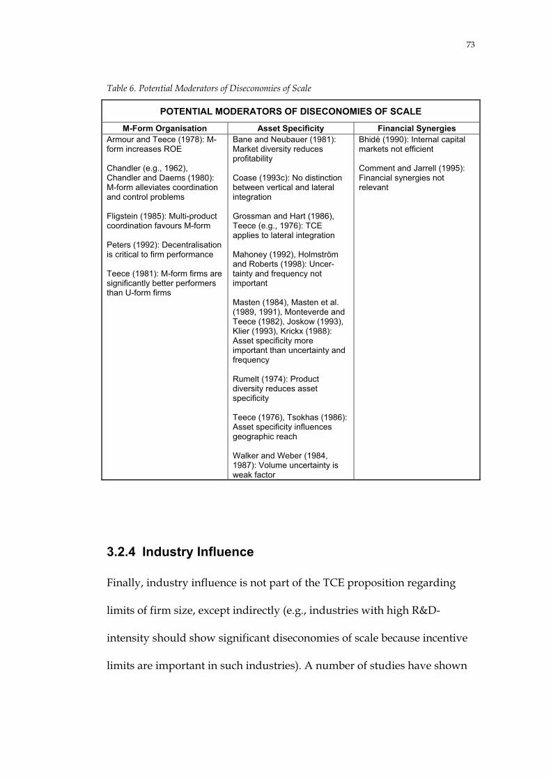
73
Table 6. Potential Moderators of Diseconomies of Scale
POTENTIAL MODERATORS OF DISECONOMIES OF SCALE
M-Form Organisation Asset Specificity Financial Synergies Armour and Teece (1978): M-form increases ROE Chandler (e.g., 1962), Chandler and Daems (1980): M-form alleviates coordination and control problems Fligstein (1985): Multi-product coordination favours M-form Peters (1992): Decentralisation is critical to firm performance Teece (1981): M-form firms are significantly better performers than U-form firms
Bane and Neubauer (1981): Market diversity reduces profitability Coase (1993c): No distinction between vertical and lateral integration Grossman and Hart (1986), Teece (e.g., 1976): TCE applies to lateral integration Mahoney (1992), Holmström and Roberts (1998): Uncer-tainty and frequency not important Masten (1984), Masten et al. (1989, 1991), Monteverde and Teece (1982), Joskow (1993), Klier (1993), Krickx (1988): Asset specificity more important than uncertainty and frequency Rumelt (1974): Product diversity reduces asset specificity Teece (1976), Tsokhas (1986): Asset specificity influences geographic reach Walker and Weber (1984, 1987): Volume uncertainty is weak factor
Bhidé (1990): Internal capital markets not efficient Comment and Jarrell (1995): Financial synergies not relevant
3.2.4 Industry Influence
Finally, industry influence is not part of the TCE proposition regarding
limits of firm size, except indirectly (e.g., industries with high R&D-
intensity should show significant diseconomies of scale because incentive
limits are important in such industries). A number of studies have shown

74
that there is weak correlation between profitability and which industry or
industries a manufacturing firm participates in. Schmalensee (1985)
suggested methods for disaggregating business-unit performance into
industry, corporate-parent and market-share effects. Rumelt (1991)
applied the method to manufacturing firms and found that industry
effects accounted for 8 per cent of the explained variance in profitability.
McGahan and Porter (1997) found a 19-per cent industry effect for all
sectors of the economy, but only 9 per cent of explained variance in
profitability for firms in the manufacturing sector (similar to Rumelt’s
findings). Thus, industry appears to influence profitability in the non-
manufacturing sector, but only slightly in the manufacturing sector. The
same appears to be true for firm growth. Hall (1986, 9) found, in an
analysis of the relationship between firm growth and size in the US
manufacturing sector, that the results were only marginally influenced by
the use of industry dummies.
The implication for the current research is that industry influences should
not be included as a variable in the statistical analyses.
3.2.5 Conclusion
This literature review indicates that the TCE framework for firm-size
limits is fairly robust. Most of the authorities support Williamson’s
75
framework, and the mechanisms behind diseconomies of scale have been
validated. The findings regarding economies of scale are somewhat
inconclusive. The two transaction cost-based moderating influences on
diseconomies of scale have both been validated. M-form firms outperform
U-form firms, at least in the manufacturing sector. Asset specificity
emerges as the most important driver of both vertical and lateral
integration.
Past research indicates that the sources of diseconomies are more
important in certain contexts. For example, atmospheric consequences and
incentive limits are especially severe in R&D-intense industries.
Communication distortion, meanwhile, is most common in diverse firms
and volatile industries. It is now possible to assess how important these
effects are, as well as how large a firm has to be before the effects
materialise. Assessing the importance of effects is at this point necessarily
qualitative, based on the collective judgement derived from the literature
review for each source of diseconomies of scale, economies of scale and
the moderating factors. Table 7 summarises this judgement. “Good/Poor”
indicates that if, for example, a firm has no problem with incentive limits,
then performance (measured as financial results) will be comparatively
good. “Importance” indicates if the effect is strong or weak. The “Impact
Size” parameter roughly indicates at what size (number of employees) the

76
effect sets in. For example, the literature review indicates that the incentive
disadvantage in R&D for large firms appears to be strong for firms with
more than 500 employees in the R&D function (see pp. 58–59, above).
“Context” shows which types of firms are most sensitive to the effects of
diseconomies of scale, economies of scale and the moderating factors.
Table 7. Extended TCE-Based “Limits of Firm Size” Framework
EXTENDED TCE-BASED “LIMITS OF FIRM SIZE” FRAMEWORK
Financial Results
Sources of Limits of Firm Size
Econo- mies of Scale
Moderators Atmos- pheric Conse-
quences
Bureau-cratic
Insularity Incentive
Limits
Commu-nication
Distortion
Organ- isation Form
Degreeof
Integra-tion
Good Low Low Low Low High M-form High Poor High High High High Low U-form Low Importance Fair Fair Fair in
general; high in, e.g., R&D
High Incon- clusive
High Asset specifi-city high;uncer-tainty low; fre-quency negli- gible
Impact Size: Small (<1,000) Medium Large (>10,000)
Weak Fair Strong
Weak Fair Strong
Weak Strong Strong
Strong Strong Strong
Strong Fair Weak
Strong Strong Strong
Strong Strong Strong
Context R&D-intense
Manage-ment/ board relation
R&D-intense
Diverse firms; unpredict-ability
Over- head-intense
The table reveals, based on Williamson’s framework and the literature
review, that all factors (except possibly economies of scale) should have a
material influence on the performance of large firms. The following
chapter builds on this finding as it translates the framework into five
testable hypotheses.

77
4. THEORETICAL FRAMEWORK AND RESEARCH HYPOTHESES
The previous chapter covered the theoretical and empirical studies—
particularly Williamson’s categorisation (1975, 117–131) of diseconomies
of scale—that inform the current research. This chapter now translates the
findings so far into five hypotheses. The hypotheses guide the quantitative
tests performed in the statistical analyses, presented in Chapter 6. In the
following, each individual hypothesis is first stated, and then discussed.
At the end of the chapter, the hypotheses are summarised and linked.
H1: Bureaucratic failure, in the form of atmospheric consequences,
bureaucratic insularity, incentive limits and communication
distortion, increases with firm size
Diseconomies of scale are bureaucratic in nature and are not easily
observed. They exist because there are diminishing returns to
management and because large firms cannot fully replicate the high-
powered incentives that exist in the market—leading to bureaucratic
failure, the opposite of market failure. Based on Williamson’s
categorisation, there are four types of diseconomies of scale: atmospheric
consequences due to specialisation, bureaucratic insularity, incentive
limits of the employment relation and communication distortion due to

78
bounded rationality. The first hypothesis postulates that these
diseconomies of scale increase with firm size.
H2: Large firms exhibit economies of scale
The theory around economies of scale is logically broken into two parts
(H2 and H4). The second hypothesis posits that ray marginal cost decreases
with firm output. This could be seen as a tautological statement, but as
was shown in Chapter 3, large firms do not necessarily benefit from
economies of scale. First, some authorities hold that economies of scale are
exhausted at relatively small firm sizes and thus the cost curve should be
flat for large firms. Second, it could be that economies of scale are available
to all participants in a market. Given these two arguments, it is important
to test whether economies of scale exist at all. That is, does ray marginal
cost decline with increased output? The hypothesis says nothing about
whether economies of scale have a material influence on firm
performance, which is expressed in the fourth hypothesis.
H3: Diseconomies of scale from bureaucratic failure have a negative
impact on firm performance
As was shown in Chapter 2, the average size of large manufacturing firms
in the United States has declined since the 1960s, relative to the total
79
economy. Thus, as large firms have become more productive they have, on
average, not been able to compensate fully for the per-unit decline in value
added by expanding into new geographic markets (reach), new product
areas (breadth), or by increasing vertical integration (depth). In line with
Stigler’s survivor principle (see p. 14, above) this indicates that the
diseconomies of scale have a material, negative influence on firm
performance. The four types of diseconomies are exhibited through lower
profitability and/or slower growth of the largest firms relative to smaller
firms, other things—such as risk—being equal.
Given this general assumption, it is also possible posit that each of the four
types of diseconomies will have a negative impact on the performance of
large firms. In the statistical analyses, the third hypothesis is broken down
into four sub-hypotheses (see also pp. 119–120, below) concerning the
negative impact on firm performance of atmospheric consequences (H3a),
bureaucratic insularity (H3b), incentive limits (H3c) and communication
distortion (H3d).
H4: Economies of scale increase the relative profitability of large firms
over smaller firms
According to TCE, unit production and transaction costs decrease with
increasing scale. However, the benefits of scale may be reaped by all

80
participants in a market, large or small, if the market is efficient. The
theoretical framework holds that this is not the case and that most
economies of scale will be proprietary to the firm in which they reside.
Thus, the hypothesis is that large firms have higher relative profitability
than small firms, other things being equal. (Note that the theoretical
framework says nothing about whether large firms grow faster than small
firms.)
H5: Diseconomies of scale are moderated by two transaction cost-
related factors: organisation form and asset specificity
The theoretical framework holds that it is possible for firms to moderate
the negative impact of diseconomies of scale. Transaction cost economics
shows that large firms benefit from multidivisional structures, while
unitary structures impede performance. Moreover, conscious choices
about the degree of integration can affect performance. In particular, firms
with a high degree of internal asset specificity will outperform those with
low internal asset specificity. Therefore, for the purposes of the statistical
analyses, the following sub-hypotheses are posited (see also p. 120, below):
large M-form firms perform better than large U-form firms (H5a); and high
internal asset specificity affects performance positively (H5b).

81
In sum, the performance of a firm depends on three influences. To begin
with, four size-related factors contribute to diseconomies of scale and
determine the firm’s size limit. Second, economies of scale increase with
firm size. Finally, two factors, M-form organisation and high asset
specificity, can moderate the diseconomies of scale. The hypotheses are
summarised in Figure 5, which also includes the theoretical framework
derived from Williamson (see Section 3.1).
Figure 5. Theoretical Framework and Hypotheses
FirmPerformance
GrowthProfitability
ModeratorsAsset Specificity
M-Form Organisation
Economies of Scale
Diseconomies of ScaleAtmospheric Consequences
Bureaucratic InsularityIncentive Limits
Communication Distortion
Size
THEORETICAL FRAMEWORK AND HYPOTHESES
H1
H2
H3
H4
H5
FirmPerformance
GrowthProfitability
ModeratorsAsset Specificity
M-Form Organisation
Economies of Scale
Diseconomies of ScaleAtmospheric Consequences
Bureaucratic InsularityIncentive Limits
Communication Distortion
SizeSize
THEORETICAL FRAMEWORK AND HYPOTHESES
H1
H2
H3
H4
H5

82
The question remains: are the hypothesised effects large enough materially
to influence the performance of a large firm? Only an empirical analysis, in
which the framework and hypotheses are operationalised, will answer
this. The next two chapters focus on this operationalisation—first by
describing the approach to the quantitative analysis, the data collected and
the measures taken to ensure reliability in the statistical analyses
(Chapter 5), and then by presenting the results of said analyses
(Chapter 6).

83
5. METHODOLOGY
This chapter turns the attention from the literature review and the
development of hypotheses to the empirical analysis. The first section
discusses the positivist approach taken in the analysis and the implications
of choosing between statistical methods. The second section moves from
this general discussion to the specifics of the data used and the quality of
the data. It finds that the data are suitable for the structural equation
modelling employed in Chapter 6.
5.1 APPROACH TO QUANTITATIVE ANALYSIS
This section gives a general impression of the analytical approach and the
method chosen for the statistical analysis. It begins with a discussion of
why a positive, quantitative approach was chosen and what the inherent
limitations of such an approach are. It then proceeds with an overview of
the use of statistical methods in similar research to explain why structural
equation modelling was used in the current research. Moreover, the
limitations of structural equation modelling are discussed. Finally, the
section compares two software packages suitable for the structural
equation modelling—Amos and LISREL—and lays out the argument for
why Amos was chosen.

84
5.1.1 Research Philosophy
The positivist approach taken here emphasises universal understanding in
Runkel and McGrath’s terms (1972, 81–89). They made the distinction
between research aimed at explaining particular phenomena and research
explaining universal phenomena. Typically, the former type of research
uses field studies or experiments, while the latter often uses surveys and
theory. According to their framework, any given research study inevitably
is a trade-off between generalisability—do the findings apply in general,
or do they only explain the situation at hand?—precision—is it reasonable
to believe that the findings are accurate?—and realism—do the findings
correspond well with the underlying reality? “Sadly, these are desirable
but not simultaneously attainable; all three—realism, precision, and
generality—cannot be maximized at the same time” (p. 115). This thesis
aims to draw general conclusions even if precision and realism are
reduced.
One could take a phenomenological approach to the research, basing it on
case studies and other qualitative methods. Cooper (1964) did so in his
often-quoted study of R&D productivity in large and small firms.
However, the current research relies on a positivist approach for reasons
found in Easterby-Smith, Thorpe and Lowe (1991, 23): This kind of
approach allows for more independence from the observations; because

85
individual or group behaviour are not the concern of this research, little
additional insight can be gained from action research or other studies in
the field. Value-freedom is important because existing studies of limits of
firm size are themselves value-laden. Causality can be deduced from the
proposed data set and manipulation, and concepts can be operationalised
to suit a positivist approach. The problem lends itself to reductionism
because the influences in the theoretical framework can be disaggregated
and independently operationalised. Moreover, as noted earlier, it should
be possible to draw generalisable conclusions based on the fairly large
sample detailed in Section 5.2. Finally, it is easier to make the necessary
cross-industry comparisons with a positivist approach.
This methodological choice means the work focuses on the facts (Easterby-
Smith, Thorpe and Lowe 1991, 27). Thus, much care was taken with the
data set and the emphasis is on looking for facts and causality rather than
underlying meaning (in a phenomenological sense). The hypotheses were
formulated before the quantitative research was carried out, rather than
deduced from the data. In addition, a large sample was used and concepts
were operationalised so that they could be measured.
There are no studies of this general type on the particular issue of
diseconomies of scale. However, generalised studies on, for example, the
profit impact of an M-form organisation or the link between size, structure

86
and complexity are widely quoted in the literature (e.g., Rumelt 1974;
Ramanujam and Varadarajan 1989). This indicates that the generalised
approach may add substantial value to the study of limits of firm size. An
added benefit is that data are available to support a generalised study.
Note that several studies have aimed at describing precisely particular
aspects of limits of firm size, as discussed in Chapter 3. Zenger’s (1989)
study of incentive limits in Silicon Valley is a good example. Several case
studies also provide realistic views of what these limits look like in action,
but in the end they have had only limited impact on academic thinking.
The notable exceptions can be found in the work on institutions in society
based on TCE, in which North was able to merge insights from case
studies with a framework for institutional change (e.g., North 1985, 1987,
1992; North and Thomas 1973). Chandler’s (e.g., 1962, 1977, 1990) work on
the evolution of large firms has also had major impact on the thinking
regarding bureaucracies.
5.1.2 Statistical Technique
This section describes the statistical technique chosen based on empirical
research precedents, the nature of the statistical task at hand, and the
specific structural equation modelling software available.

87
5.1.2.1 Empirical Precedents
As discussed earlier, general statistical analyses of diseconomies of scale
have not been attempted before, except for simple direct comparisons
between firm size and performance. There are, however, a number of
empirical studies of particular aspects of the limits of firm size or of
general TCE problems. These offer guidance on the choice of statistical
methods for the current research and the operationalisation of variables.
There are two basic types of quantitative statistical analysis: older, non-
regression-based analyses and newer, regression-based analyses. This
section considers the statistical approaches taken in a number of these
studies. The intent is not to discuss particular findings, but rather to
inform the choice of statistical method for the current research.
Early inquiries (e.g., McConnell 1945; Stigler 1958) into relationships
between profitability and firm size made simple comparisons between the
dependent variable (profitability) and independent variable (size), using
histograms with the size-bracket as the categorising variable. At best, these
analyses indicated that relationships between the variables existed, but
because they did not include modern tests of statistical significance, they
left many questions unanswered.
Later, researchers including Rumelt (1974), Teece (1981) and Palepu (1985),
used comparisons of samples to demonstrate statistical significance. Their

88
methods ranged from simple comparisons of average profitability for two
samples, to sophisticated tests of the statistical significance of the
differences using parametric (t-test) and non-parametric (median and
Mann-Whitney U-test) methods (Palepu 1985, 245–246). However, these
techniques probably did not extract the full information content of the
samples. For example, Rumelt later used a regression technique when he
updated his analysis of diversification and structure (Rumelt 1982).
Yet another statistical approach is to study the amount of variance
extracted. Schmalensee (1985) used analysis of variance (ANOVA),
arguing that: ”This study employs a simple analysis of variance
framework that allows us to focus on the existence and importance of firm,
market, and market share effects without having to deal simultaneously
with specific hypotheses and measurement issues related to their
determinants”. Put differently, analysis of variance is an excellent tool for
exploratory analysis. Other examples of related studies employing
ANOVA include Rumelt (1991) and McGahan and Porter (1997).
Finally, most statistical analyses over the last 35 years relating to aspects of
diseconomies of scale have used multivariate regression techniques
(Armour and Teece 1978; Aw and Batra 1998; Child 1973; Comment and
Jarrell 1995; Fligstein 1985; Kwoka 1980; Levy 1981; Lucas 1978; Mahoney
1989; Masten 1984; Masten, Meehan and Snyder 1989, 1991; Olson 1982;

89
Pondy 1969; Pugh et al. 1969; Rasmusen and Zenger 1990; Rumelt 1982;
Rumelt and Wensley 1981; Walker and Weber 1984, 1987; Zenger 1994).
They ranged from simple regressions to complex structural equation
models, and were used for both exploratory and confirmatory analyses.
This brief overview indicates that researchers have increasingly used
sophisticated statistical techniques, usually leading to multivariate
methods of analysis. Stigler’s survivor principle (see p. 14, above) suggests
that the added complexity of using these techniques is more than
compensated for by the added insights they bring; otherwise researchers
would not continue to employ them and the techniques would not
survive. It is also true that the simpler techniques have more or less
disappeared from the literature as statistical methods have evolved and
computing power available to researchers has increased.
5.1.2.2 Selection of Statistical Technique
The current research uses multivariate analysis. As early as 1966, Gatty
argued that “for the purposes of…any…applied field, most of our tools
are, or should be, multivariate. One is pushed to a conclusion that unless
a…problem is treated as a multivariate problem, it is treated superficially”
(1966, 158). Or as Hardyck and Petrinovich put it ten years later:

90
“Multivariate analysis methods will predominate in the future…”
(1976, 7). This has been born out over the last 25 years.
Among different multivariate techniques, structural equation modelling
(SEM) was picked based on Hair et al.’s classification scheme for choosing
among techniques (1998, 20–21) and a review of the pertinent literature on
SEM (Bollen 1989, 1–9; Kelloway 1998, 2–3; Maruyama 1998, 20–24). SEM
is the most appropriate technique when multiple relationships between
dependent and independent variables are studied. Moreover, SEM is well
suited for confirmatory analysis and allows for efficient hypothesis testing,
especially of complex models. Finally, SEM allows for the use of latent,
unobserved variables. As will be discussed in Chapter 6, these three
attributes are important in the current research.
Structural equation modelling must be used judiciously, however. A
number of criticisms of this technique have been summarised by
Maruyama (1998, 272–278). SEM cannot be used to confirm a model. It can
only fail to disprove it. This makes replicability important, and this is a
key reason for using publicly available data in the statistical analyses
described in Chapter 6. Related to this is the risk of inferring causality
where none exists. Strong correlation does not imply causality. For this
reason, the path diagrams used in the next chapter reveal causalities based
on theory, not on a study of correlation.

91
In addition, incorrect operationalisation and naming of variables
(especially latent variables) can lead to erroneous conclusions. In
Maruyama’s words, “giving something a name does not necessarily make
it what we call it or ensure that we understand the thing we have named”
(p. 273). This is certainly a valid point for the present work. For example,
incentive limits were operationalised, based on the theory, with relative
R&D expense. But does this mean that the SEM model truly captures
incentive limits, or does it merely capture relative R&D expense?
Finally, SEM has often been used for model development rather than
model confirmation. The current research has tried to avoid this by using
path diagrams that have been derived directly from the theoretical
framework, as expressed in the hypotheses.
5.1.2.3 Amos versus LISREL
Amos was used in the current research, instead of the more recognised
LISREL SEM software package. 23 LISREL certainly has a much larger
installed base and thousands of references in the literature. Amos is less
well known and has only been cited in 56 references as of the year 2000,
according to its vendor (SmallWaters 2000). Amos, however, is much
23 Information on Amos is available at http://www.smallwaters.com.

92
easier to use for the occasional statistician because it is based on
interactive, graphical path diagrams; it is gaining ground among
researchers for this reason. More important, Amos has one attribute that
serves this particular research effort well: its ability to handle missing
values in the data collected.
LISREL uses pair-wise or list-wise deletion to handle missing data. Amos,
on the other hand, uses full-information maximum likelihood (FIML)
estimation, arguably a leading-edge technique (Arbuckle 1996). When data
are missing completely at random, the list-wise or pair-wise deletion
methods employed by LISREL are asymptotically equivalent to FIML, but
the standard errors of the parameter estimates can be considerably larger
for LISREL. This means that Amos makes more efficient use of the
observations, a critical consideration in the current research because the
number of large firms is limited and the sample size could not be
expanded infinitely. Moreover, if data are not missing at random, the
Amos FIML estimates tend to be less biased than when pair-wise or list-
wise deletions are used. Note that FIML does not impute missing values;
instead Amos calculates the likelihood of the parameters based on each
observed case.
The major advantage of LISREL is that it sometimes handles ordinal data
more correctly with polychoric or polyserial correlations. As is discussed
93
in Chapter 6, two variables are ordinal in this research.24 The only way
Amos can handle ordinals is by treating them as continuous variables,
which often leads to biased estimates, or by importing the covariance
matrix from another SEM package, which eliminates the advantage of
FIML estimation. The bias when treating ordinals as continuous variables
is usually towards underestimates of coefficients and overestimates of
standard errors and chi-square (Bollen 1989, 433–446). This suggests that
Amos in most cases will underestimate a model’s fit. There is no suitable
remedy for this in the present case (and usually not in other cases).
LISREL’s weighted-least-square (WLS) approach with polychoric or
polyserial correlations handles ordinals well if the underlying
distributions are normal. This is definitely the case for one of the ordinals
in the current research, and may be the case for the other ordinal.25 Yet
some critics have argued that effective use of polychoric and polyserial
correlation requires 2000 to 5000 observations (Yung and Bentler 1994), a
number well beyond the sample available here. Indeed, Jöreskog and
Sörbom, the creators of LISREL, concur with this opinion: “A poorly
estimated asymptotic covariance matrix, such as estimated from a small
sample, can do more harm than good, when used with WLS. If the sample
24 The variables describe the level of vertical integration and divisionalisation. That is, they affect
the TCE-based moderators (asset specificity and M-form), but do not relate to diseconomies of scale.
25 See further discussion in Footnote 39 (p. 166) and Footnote 41 (p. 171), below.

94
size is not sufficiently large to produce an accurate estimate of the
asymptotic covariance matrix, it is probably better to use ML” (1996, 239).
Thus, one can either use Amos and treat ordinal data as continuous data,
or use LISREL with a sample size that is too small—neither of which are
optimal approaches. For the purposes of this research, a choice was made
to use Amos because of its other positive attributes, but no attempt was
made to compare which software package would handle the ordinal data
best, or if this really would make a difference. The choice is in line with
Wothke26 (1997), who recommends that for sample sizes smaller than 2000,
“your best bet would be to treat the ordinal data as continuous”, and with
Hayduk (1996, 213), who claims that the continuous-data assumption is of
little practical significance: “ordinal variables have continued to receive
considerable attention, though the problems may not be as serious as
popular opinion suggests.”
Finally, choosing Amos and the existence of missing data made two more
choices automatic. Alternative estimation techniques such as generalised
least squares and asymptotically distribution-free (ADF) estimation could
not be used, because they do not allow missing data. ADF might otherwise
have been useful, because it handles non-normality well. In addition,
26 Co-creator of Amos.

95
Amos does not allow bootstrapping when data are missing. Bootstrapping
might otherwise have increased the reliability of the analysis, because it
reduces the impact of non-normality. Fortunately, as will be discussed in
Section 5.2.3, non-normality is not a major issue in the current analyses.

96
5.2 DATA OVERVIEW
This section discusses the data used in the statistical model. The first part
of the section defines the variables and discusses data sources. The
following part tests the sample data for inconsistencies and outliers and
then reviews the sample sizes. The final part transforms the variables
using commonly accepted transformation techniques and then tests the
data for heteroscedasticity, linearity and other potential problems. The
conclusion is that the sample data are reasonably well-behaved and are
suitable for further analysis.
Throughout this section, reference is made to two sub-models: (a) the
relationship between size and diseconomies of scale and economies of
scale; and (b) the impact of diseconomies of scale, economies of scale and
moderating factors on firm performance. These sub-models are used in the
statistical analyses in Chapter 6.
5.2.1 Definitions and Sources
The conducted analyses were cross-sectional. Data were collected for
publicly traded manufacturing firms (SIC codes 10–39) with headquarters
in the US and with sales of more than $500 million. The benchmark period

97
was 1998. All data are available for downloading at http://canback.com/
henley.htm in the files Source98.xls and Source98.sav.
1998 saw high economic growth, but it was not a peak in the business
cycle. Table 8 shows key indicators for the time period surrounding the
year and the rank of the indicator for the time period 1961–2000.
Table 8. Select Economic Indicators for the United States
SELECT ECONOMIC INDICATORS FOR THE UNITED STATES
Indicator 1996 1997 1998 1999 2000 ’61–’00 Rank GDP Growth (%) 3.6 4.4 4.3 4.1 4.1 Medium: 15 of 40 Mfg. GDP Growth (%) 2.4 5.4 4.1 6.1 4.1 Medium: 14 of 40 Mfg. Return on Equity (%) 16.7 16.7 15.8 16.4 15.1 High: 7 of 40 Mfg. Capacity Utilisation (%) 81.6 82.7 81.4 80.6 80.7 Medium: 20 of 40 Inflation (%) 3.0 2.3 1.6 2.2 3.4 Low: 34 of 40 Source: Council of Economic Advisers (2002)
The analyses ultimately involved 14 variables. Of these, 9 were direct
variables and 5 were calculated from other direct variables. For example,
the calculated variable ROE was determined by dividing two direct
variables: Net Income and Equity. Direct, on the other hand, implies that
the variable was taken directly from one of the data sources. To create the
5 calculated variables, an additional 10 direct variables were used. Thus,
the analyses encompassed a total of 19 (9+10) direct variables. Moreover,
44 other variables were collected although they were not used in the final
analysis.

98
Primary and secondary data were collected from several sources,
including company organisation charts, official filings such as 10-Ks and
proxy statements,27 annual reports, biographies of executives, historical
company documents, corporate web sites, articles in Business Week and
Fortune, corporate watchdogs such as the Investor Responsibility Research
Center (IRRC), Compustat and academic research.
Table 9 depicts the 14 variables used. Specific information about the
variables appears under each analysis section in Chapter 6.
Table 9. Overview of Variables Used in the Analyses
OVERVIEW OF VARIABLES USED IN THE ANALYSES
Usea Nameb Labelc Type Description Metric Sources Size (a) empl Employeesd Direct No. of employees ’000 Compustat Diseconomies of Scale (a, b)
ulabour Atmospheric Consequences
Calculated Unit labour cost defined as labour cost � employees [ulabour = labour � empl]
$’000
Diseconomies of Scale (a, b)
tenure Leadership Tenure
Direct Average years of employment with firm for officers
Years 10-Ks, proxy statements. annual reports, corporate web sites, executive biographies
Diseconomies of Scale (a, b)
age Company Age Direct Years since founding of company
Years 10-Ks, proxy statements. annual reports, corporate web sites, historical sources
27 Filings with the United States Securities and Exchange Commission: the 10-K is the full annual
report and usually differs in content from the company’s shareholder annual report; proxy statements (report DEF 14A) contain information pertaining to voting at security holders’ meetings (annual meetings or special meetings). Available from EDGAR at http://www.sec.gov/.

99
Usea Nameb Labelc Type Description Metric Sources Diseconomies of Scale (a, b)
rd Incentive Limits Calculated Research and development expense � Sales [rd = rdexp � sales]
%
Diseconomies of Scale (a, b)
levels Communication Distortion
Direct No. of hierarchical levels
# Annual reports, corporate web sites, 10-Ks, company organisation charts
Economies of Scale (a, b)
fixhigh Economies of Scale
Calculated Defined as (fixed cost)2 � sales [fixhigh = fixexp2 � sales]
$M
Moderators (b) foreign Geographic Reach
Direct % of sales derived outside the United States
% Compustat, annual reports, 10-Ks
Moderators (b) dr Product Breadth Calculated Defined as the diversification ratio (1 � Rumelt’s specialisation ratio) = % of sales not related to the company’s core activities [dr = 1 � sr]
%
Moderators (b) vert Vertical Depth Direct 2 = Very high; 1 = High; 0 = Average or low
Ordinal 10-Ks, annual reports, corporate web sites, Compustat
Moderators (b) govern Governance Direct Qualitative rankings
Index Business Week, IRRC, Fortune
Moderators (b) div Divisionalisation Direct 2 = Divisionalised; 1 = Hybrid; 0 = Unitary
Ordinal 10-Ks, proxy statements, annual reports, corporate web sites
Performance (b)
growth Growthd Direct 5-year compound annual growth rate (1993–1998)
% Compustat
Performance (b)
eva Profitabilityd Calculated Economic value added defined as return on equity (ROE) less cost of equity (COE) [eva = roe � coe]
%
a a and b in the “Use” column indicate whether the variable is used in sub-models a or b b The “Name” column shows the name given to the variable in SPSS and in Amos c The “Label” column shows the label given to the variable in SPSS and in Amos d Appendix B discusses other definitions of size and performance

100
Table 10 below gives further definitions for those variables that were
calculated from other (direct) variables. The table includes the 10
additional direct variables discussed above, as well as variables used to
support the main analyses in Chapter 6 (see also Appendix B).
Table 10. Overview of Supporting Variables
OVERVIEW OF SUPPORTING VARIABLES
Usea Nameb Labelc Type Description Metric Sources Diseconomies of Scale (a, b)
labour Labour Direct Labour cost $M Compustat
Diseconomies of Scale (a, b)
rdexp R&D Direct Research and development expense
$M Compustat
Diseconomies of Scale (a, b)
sales Sales Direct Revenue $M Compustat
Economies of Scale (a, b)
fixexp Fixed Cost Calculated Fixed cost defined as SG&A + depreciation + interest [fixexp = sgaexp + depr + int]
$M
Economies of Scale (a, b)
sgaexp SG&A Direct Selling, general and administrative expense
$M Compustat
Economies of Scale (a, b)
depr Depreciation Direct Depreciation $M Compustat
Economies of scale (a, b)
int Interest Direct Interest expense % Compustat
Moderators (b) sr Specialisation Ratio
Calculated Defined as share of sales derived from core business = core sales � sales [sr = csales � sales]
%
Moderators (b) csales Core Sales Direct Core sales defined as sales derived from the firm’s main SIC code
$M Compustat, annual reports, 10-Ks, corporate web sites
Moderators (b) vi VI% Calculated Vertical integration defined as value added � factor costs [vi = va � factor]
Moderators (b) factor Factor Costs Calculated Factor costs defined as sales � net income + cost of equity · equity [sales � ni + (coe · equity)]
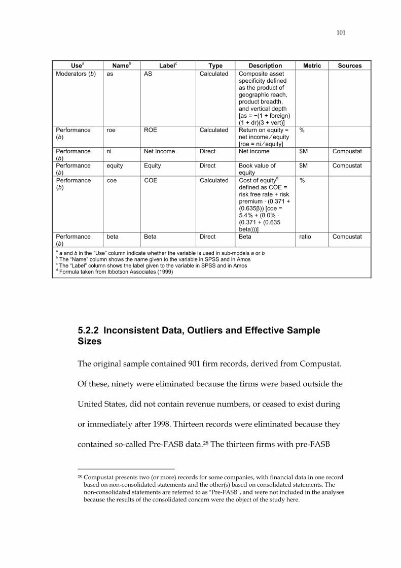
101
Usea Nameb Labelc Type Description Metric Sources Moderators (b) as AS Calculated Composite asset
specificity defined as the product of geographic reach, product breadth, and vertical depth [as = �(1 + foreign) (1 + dr)(3 + vert)]
Performance (b)
roe ROE Calculated Return on equity = net income � equity [roe = ni � equity]
%
Performance (b)
ni Net Income Direct Net income $M Compustat
Performance (b)
equity Equity Direct Book value of equity
$M Compustat
Performance (b)
coe COE Calculated Cost of equityd defined as COE = risk free rate + risk premium · (0.371 + (0.635�)) [coe = 5.4% + (8.0% · (0.371 + (0.635 beta)))]
%
Performance (b)
beta Beta Direct Beta ratio Compustat
a a and b in the “Use” column indicate whether the variable is used in sub-models a or b b The “Name” column shows the name given to the variable in SPSS and in Amos c The “Label” column shows the label given to the variable in SPSS and in Amos d Formula taken from Ibbotson Associates (1999)
5.2.2 Inconsistent Data, Outliers and Effective Sample Sizes
The original sample contained 901 firm records, derived from Compustat.
Of these, ninety were eliminated because the firms were based outside the
United States, did not contain revenue numbers, or ceased to exist during
or immediately after 1998. Thirteen records were eliminated because they
contained so-called Pre-FASB data.28 The thirteen firms with pre-FASB
28 Compustat presents two (or more) records for some companies, with financial data in one record
based on non-consolidated statements and the other(s) based on consolidated statements. The non-consolidated statements are referred to as "Pre-FASB", and were not included in the analyses because the results of the consolidated concern were the object of the study here.

102
data also had regular records that were kept in the sample. Four firms
with revenues less than $500 million were eliminated. Six limited
partnerships were eliminated because their records did not contain
enough information to be of interest. Six firms had duplicate records. One
firm had recently been spun out from its corporate parent and did not
provide meaningful data. Thus, the final sample contained 784 firm
records.
For these 784 records, each variable was first screened for inconsistent
data; then outliers were eliminated if a rationale for exclusion was found.
The following are examples of inconsistent data found in the records:
negative equity, zero foreign sales of well-known international companies,
negative beta and negative market value.
Outliers were identified by standardising the variables and then
identifying those records which fell more than three standard deviations
from the mean, in line with Hair et al. (1998, 65). Those outliers for which
the data made sense were kept, while, again, inconsistent data were
eliminated. All changes to the original database described above can be
found in the file Source98.xls at http://canback.com/henley.htm. Table 11
shows the number of outliers retained in the database.

103
Table 11. Overview of Outliers
OVERVIEW OF OUTLIERS
Variable No. of Outliers
before Screening No. of Outliers after Screening
Employees 0 0 Atmospheric Consequences 2 2 Leadership Tenure 0 0 Company Age 2 2 Incentive Limits 0 0 Communication Distortion 3 3 Economies of Scale 9 8 Geographic Reach 0 0 Product Breadth 20 20 Vertical Depth not meaningful (ordinal) Governance 4 4 Divisionalisation not meaningful (ordinal) Growth 9 6 Profitability 5 4
Multivariate outliers were detected using DeCarlo’s macro (1997)
normtest.sps for SPSS. This macro calculates, among other things, the
Mahalanobis D2 measure. Missing values were assigned the mean for the
variable. The results are summarised in Table 12.
Table 12. Multivariate Outliers
MULTIVARIATE OUTLIERS
No. of Outliers
before Screening No. of Outliers after Screening
Sub-Model a 4 4 Sub-Model b 7 7
Eleven cases could have been considered outliers, if a significance
exceeding 0.01 was used as the hurdle for critical F. However, in none of
the cases was there a compelling reason to exclude the observation.

104
Tables 13 and 14 show the effective sample sizes for the two sub-models
after the screening.
Table 13. Effective Sample Sizes for Sub-Model a
EFFECTIVE SAMPLE SIZES FOR SUB-MODEL A
Empl
oyee
s
Atm
osph
eric
C
onse
quen
ces
Lead
ersh
ip
Tenu
re
Com
pany
Age
Ince
ntiv
e Li
mits
Com
mun
icat
ion
Dis
tort
ion
Econ
omie
s of
Sc
ale
Employees 784 Atmospheric Consequences 146 146 Leadership Tenure 163 57 163 Company Age 638 145 153 638 Incentive Limits 489 108 111 419 489 Communication Distortion 386 137 123 347 258 386 Economies of Scale 752 143 155 612 473 374 752
Table 14. Effective Sample Sizes for Sub-Model b
EFFECTIVE SAMPLE SIZES FOR SUB-MODEL B
Atm
osph
eric
C
onse
quen
ces
Lead
ersh
ip
Tenu
re
Com
pany
Age
Ince
ntiv
e Li
mits
Com
mun
icat
ion
Dis
tort
ion
Econ
omie
s of
Sc
ale
Geo
grap
hic
R
each
Prod
uct B
read
th
Vert
ical
Dep
th
Gov
erna
nce
Div
isio
nalis
atio
n
Gro
wth
Prof
itabi
lity
Atmospheric Consequences 146 Leadership Tenure 57 163 Company Age 145 153 638 Incentive Limits 108 111 419 489 Communication Distortion 137 123 347 258 386 Economies of Scale 143 155 612 473 374 752 Geographic Reach 134 143 553 412 343 642 663 Product Breadth 131 152 565 423 348 650 594 670 Vertical Depth 133 152 569 424 350 655 596 670 675 Governance 73 74 214 162 172 223 205 209 211 229 Divisionalisation 135 119 337 252 372 364 333 340 341 166 375 Growth 143 157 614 472 374 725 644 646 651 228 363 756 Profitability 145 162 636 489 384 751 663 670 674 229 373 753 781

105
The tables show that all variables except for 2 had more than 200
observations; 9 out of 14 variables had more than 400 observations (see the
diagonals). On average, sub-model a contained 480 observations and sub-
model b contained 517 observations. The fairly low number of
observations for Atmospheric Consequences (146) and Leadership
Tenure (163) reduces the integrity of the upcoming analyses, but far from
a point where they become meaningless.
According to Hair et al. (1998, 604–605), four criteria determine an
appropriate sample size. When maximum likelihood estimation is used, as
here, a minimum sample size of 100 to 150 is recommended. Sample sizes
of more than 400 or 500 often become “too sensitive”. Hair et al.
recommends a sample size of 200 as a starting point. In addition, the
sample size should be at least five times the number of parameters
estimated. The most important sub-model in this analysis (b) had 13
variables and thus a maximum of 91 parameters (13 variances and 78
covariances) were estimated, requiring at least 455 observations—close to
the 396 average number of observations actually available. More
observations are required if misspecification is suspected or if data are
strongly non-normal (not the case here, as was shown in Section 5.2.3).
Sub-model a met the requirement more easily (28 parameters, 140
observations required, 455 average number of observations available).

106
The sample-size tables also indicate that most covariances had a
reasonable number of observations. Again, Hair et al. (1998, 604–605)
recommends a minimum of 100 to 150 observations. In sub-model b, only
Atmospheric Consequences / Leadership Tenure (57), Atmospheric
Consequences / Governance (73) and Leadership Tenure / Governance
(74) had less than 100 observations, while 17 of 78 covariances had less
than 150 observations. There was an average of 353 observations per
covariance in sub-model b. Sub-model a included 7 of 21 covariances with
less than 150 observations and one came with less than 100: Atmospheric
Consequences / Leadership Tenure (57). There were an average of 295
observations per covariance in sub-model a.
Because a significant number of observations were missing, their
randomness had to be tested. The test was made by calculating
dichotomised variable correlations. Each variable (except for Employees,
which had no missing values) was recoded with the value 1 if the data
existed, and 0 if the data was missing (Hair et al. 1998, 60). Table 15 shows
the resulting correlations. For low correlations, the data can be considered
missing completely at random (MCAR)—and most correlations were low
in this analysis. Two correlations exceeded 0.4, signifying moderate non-
randomness; one correlation exceeded 0.9, signifying strong non-
randomness. The strong non-randomness of Communication Distortion /

107
Divisionalisation is unsurprising: the data were collected simultaneously
for the two variables.
Table 15. Multivariate Test for Missing Completely at Random (MCAR)
MULTIVARIATE TEST FOR MISSING COMPLETELY AT RANDOM (MCAR)
Atm
osph
eric
C
onse
quen
ces
Lead
ersh
ip
Tenu
re
Com
pany
Age
Ince
ntiv
e Li
mits
Com
mun
icat
ion
Dis
tort
ion
Econ
omie
s of
Sc
ale
Geo
grap
hic
Rea
ch
Prod
uct B
read
th
Vert
ical
Dep
th
Gov
erna
nce
Div
isio
nalis
atio
n
Gro
wth
Prof
itabi
lity
Atmospheric Consequences 1 Leadership Tenure 0.22 1 Company Age 0.22 0.16 1 Incentive Limits 0.11 0.06 0.14 1 Communication Distortion 0.43 0.27 0.22 0.09 1 Economies of Scale 0.05 �0.02 0.00 0.05 0.05 1 Geographic Reach 0.10 0.04 0.12 �0.01 0.12 0.11 1 Product Breadth 0.06 0.11 0.18 0.04 0.13 0.13 0.27 1 Vertical Depth 0.07 0.11 0.19 0.02 0.13 0.14 0.26 0.97 1 Governance 0.22 0.18 0.20 0.11 0.33 0.05 0.09 0.11 0.11 1 Divisionalisation 0.43 0.26 0.21 0.10 0.96 0.06 0.11 0.14 0.13 0.32 1 Growth 0.04 0.00 �0.02 0.01 0.02 0.00 0.09 0.00 0.00 0.11 0.02 1 Profitability �0.02 �0.02 0.02 0.08 �0.02 0.20 0.15 0.15 0.09 0.04 �0.02 �0.01 1Note: Figures show dichotomised correlations
5.2.3 Data Transformation, Non-Normality, Heteroscedasticity and Linearity
Most continuous variables were transformed to reach more univariate
normal distributions. This was done by studying histograms for each
variable and by analysing the skewness and kurtosis statistics. A
Kolmogorov-Smirnov (with the Lilliefors modification) normality test was

108
also performed. Those variables that deviated significantly from normal
distribution were transformed. The transformations were based on the
standard approach of using the square root for mild non-normality, the
logarithm for moderate non-normality, and the inverse for severe non-
normality. In addition, in some instances the arctangent transformation
was used to reduce kurtosis. Table 16 summarises the transformations
used. While the use of transformations increases the accuracy of the test
statistics, it sometimes makes it more difficult to interpret the results for
each variable because scales change and the variable itself make take on a
new meaning (Hair et al. 1998, 78). The current research is not concerned
with the variables’ scales and thus the data transformations on balance
benefit the statistical analysis.
Table 16. Overview of Transformation Formulas
OVERVIEW OF TRANSFORMATION FORMULAS
Variable Transformation Employees atan(0.67(sqrt(ln(Employees · 1000)) � mean) � sdev);
mean = 2.9956; sdev = 0.18056 Atmospheric Consequences sqrt(Atmospheric Consequences) Leadership Tenure none Company Age none Incentive Limits ln(Incentive Limits + 0.001) Communication Distortion ln(Communication Distortion) Economies of Scale ln(Economies of Scale) Geographic Reach ln(1 + Geographic Reach) Product Breadth ln(1 + Product Breadth) Vertical Depth none Governance �1000 � Governance Divisionalisation none Growth atan(0.5(ln(Growth + 0.35) + 0.9) � sdev); sdev = 0.30597 Profitability atan(0.9(Profitability � 2.432) � sdev); sdev = 17.847

109
The skewness, kurtosis and Kolmogorov-Smirnov statistics are listed
below in Tables 17 and 18. In general, the variables exhibited mild to
severe skewness and kurtosis before the transformations, while most of
them were normal at the 5 per cent confidence level after transformations.
Table 17 shows the statistics before transformation. Most untransformed
variables were non-normal at the 1 per cent probability level (z<2.58). The
Kolmogorov-Smirnov z was larger than the often-used benchmark 2.0 for
7 of 12 variables.
Table 17. Univariate Normality Statistics for Untransformed Variables
UNIVARIATE NORMALITY STATISTICS FOR UNTRANSFORMED VARIABLES
Variable Skewness Kurtosis Kolmogorov-
Smirnov z Statistic SE z Statistic SE z Employees 8.78 0.09 100.50 115.40 0.17 661.68 8.96Atmospheric Consequences 0.32 0.20 1.61 0.23 0.40 0.58 0.60Leadership Tenure 0.19 0.19 0.99 �0.74 0.38 1.96 0.83Company Age 0.74 0.10 7.63 2.06 0.19 10.67 1.35Incentive Limits 2.60 0.11 23.51 8.14 0.22 36.94 4.94Communication Distortion 0.24 0.12 1.91 �0.05 0.25 0.20 1.10Economies of Scale 5.48 0.09 61.45 35.68 0.18 200.39 9.54Geographic Reach 0.77 0.09 8.16 0.24 0.19 1.26 3.55Product Breadth 0.37 0.09 3.91 �1.25 0.19 6.63 4.99Vertical Depth not meaningful (ordinal) Governance 0.96 0.16 5.95 1.22 0.32 3.81 1.46Divisionalisation not meaningful (ordinal) Growth 2.11 0.09 23.68 9.52 0.18 53.60 3.72Profitability �0.04 0.09 0.51 5.13 0.17 29.33 2.74Note: SE = Standard Error

110
Table 18 shows the statistics after transformation. All variables, except for
Geographic Reach and Product Breadth, had Kolmogorov-Smirnov z
below (or close) to 2; the skewness z and kurtosis z were usually less than
2.58. Thus, the variables were close to normally distributed.
Table 18. Univariate Normality Statistics for Transformed Variables
UNIVARIATE NORMALITY STATISTICS FOR TRANSFORMED VARIABLES
Variable Skewness Kurtosis Kolmogorov-
Smirnov z Statistic SE z Statistic SE z Employees 0.16 0.09 1.86 �0.80 0.17 4.59 1.28Atmospheric Consequences �0.07 0.20 0.32 0.11 0.40 0.29 0.59Leadership Tenure �0.33 0.19 1.76 �0.55 0.38 1.45 0.85Company Age �0.23 0.10 2.37 �0.22 0.19 1.12 2.25Incentive Limits �0.02 0.11 0.20 �0.39 0.22 1.78 0.76Communication Distortion �0.08 0.12 0.63 0.04 0.25 0.16 0.71Economies of Scale 0.28 0.09 3.17 0.07 0.18 0.42 0.82Geographic Reach 0.77 0.09 8.16 0.24 0.19 1.26 3.37Product Breadth 0.37 0.09 3.91 �1.25 0.19 6.63 5.24Vertical Depth not meaningful (ordinal) Governance �0.05 0.16 0.28 0.23 0.32 0.73 0.64Divisionalisation not meaningful (ordinal) Growth �0.10 0.09 1.08 0.15 0.18 0.86 0.84Profitability 0.21 0.09 2.38 �0.16 0.17 0.93 0.57 Note that neither Geographic Reach nor Product Breadth could be further
improved because they had severely non-normal distributions (Figure 6).
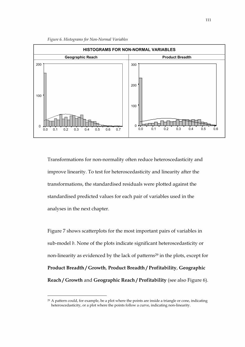
111
Figure 6. Histograms for Non-Normal Variables
HISTOGRAMS FOR NON-NORMAL VARIABLES
Geographic Reach Product Breadth
Transformations for non-normality often reduce heteroscedasticity and
improve linearity. To test for heteroscedasticity and linearity after the
transformations, the standardised residuals were plotted against the
standardised predicted values for each pair of variables used in the
analyses in the next chapter.
Figure 7 shows scatterplots for the most important pairs of variables in
sub-model b. None of the plots indicate significant heteroscedasticity or
non-linearity as evidenced by the lack of patterns29 in the plots, except for
Product Breadth / Growth, Product Breadth / Profitability, Geographic
Reach / Growth and Geographic Reach / Profitability (see also Figure 6).
29 A pattern could, for example, be a plot where the points are inside a triangle or cone, indicating
heteroscedasticity, or a plot where the points follow a curve, indicating non-linearity.
0.70.60.50.40.30.20.10.0
200
100
00.70.60.50.40.30.20.10.0
200
100
00.60.50.40.30.20.10.0
300
200
100
00.60.50.40.30.20.10.0
300
200
100
0

112
Box’s M, the standard test for assessing heteroscedasticity, was calculated
for these four covariances. Table 19 shows that only Geographic Reach /
Profitability had a problematic significance when the standard benchmark
of 0.01 was used (Hair et al. 1998, 328).
Figure 7. Heteroscedasticity and Linearity Analysis
HETEROSCEDASTICITY AND LINEARITY ANALYSIS
Dependent Variable: GrowthIndependent Variable: Atmospheric Consequences
Standardised Predicted Value
3210-1-2-3
Stan
dard
ised
Res
idua
l
2
1
0
-1
-2
-3
-4
Dependent Variable: GrowthIndependent Variable: Atmospheric Consequences
Standardised Predicted Value
3210-1-2-3
Stan
dard
ised
Res
idua
l
2
1
0
-1
-2
-3
-4
Standardised Predicted Value
3210-1-2-3
Stan
dard
ised
Res
idua
l3
2
1
0
-1
-2
Dependent Variable: ProfitabilityIndependent Variable: Atmospheric Consequences
Standardised Predicted Value
3210-1-2-3
Stan
dard
ised
Res
idua
l3
2
1
0
-1
-2
Dependent Variable: ProfitabilityIndependent Variable: Atmospheric Consequences
Standardised Predicted Value
3210-1-2
Stan
dard
ised
Res
idua
l
2
1
0
-1
-2
-3
Dependent Variable: GrowthIndependent Variable: Leadership Tenure
Standardised Predicted Value
3210-1-2
Stan
dard
ised
Res
idua
l
2
1
0
-1
-2
-3
Dependent Variable: GrowthIndependent Variable: Leadership Tenure
Standardised Predicted Value
210-1-2-3
Stan
dard
ised
Res
idua
l
3
2
1
0
-1
-2
-3
Dependent Variable: ProfitabilityIndependent Variable: Leadership Tenure
Standardised Predicted Value
210-1-2-3
Stan
dard
ised
Res
idua
l
3
2
1
0
-1
-2
-3
Dependent Variable: ProfitabilityIndependent Variable: Leadership Tenure

113
Standardised Predicted Value
3210-1-2-3-4
Stan
dard
ised
Res
idua
l
3
2
1
0
-1
-2
-3
-4-5
Dependent Variable: GrowthIndependent Variable: Company Age
Standardised Predicted Value
3210-1-2-3-4
Stan
dard
ised
Res
idua
l
3
2
1
0
-1
-2
-3
-4-5
Dependent Variable: GrowthIndependent Variable: Company Age
Standardised Predicted Value
43210-1-2-3
Stan
dard
ised
Res
idua
l
4
3
2
1
0
-1
-2
-3
Dependent Variable: ProfitabilityIndependent Variable: Company Age
Standardised Predicted Value
43210-1-2-3
Stan
dard
ised
Res
idua
l
4
3
2
1
0
-1
-2
-3
Dependent Variable: ProfitabilityIndependent Variable: Company Age
Standardised Predicted Value
3210-1-2-3
Stan
dard
ised
Res
idua
l
3
2
1
0
-1
-2
-3
-4
Dependent Variable: GrowthIndependent Variable: Incentive Limits
Standardised Predicted Value
3210-1-2-3
Stan
dard
ised
Res
idua
l
3
2
1
0
-1
-2
-3
-4
Dependent Variable: GrowthIndependent Variable: Incentive Limits
Standardised Predicted Value
3210-1-2-3
Stan
dard
ised
Res
idua
l
3
2
1
0
-1
-2
-3
Dependent Variable: ProfitabilityIndependent Variable: Incentive Limits
Standardised Predicted Value
3210-1-2-3
Stan
dard
ised
Res
idua
l
3
2
1
0
-1
-2
-3
Dependent Variable: ProfitabilityIndependent Variable: Incentive Limits
Standardised Predicted Value
3210-1-2-3-4
Stan
dard
ised
Res
idua
l
3
2
1
0
-1
-2
-3
Dependent Variable: ProfitabilityIndependent Variable: Communication Distortion
Standardised Predicted Value
3210-1-2-3-4
Stan
dard
ised
Res
idua
l
3
2
1
0
-1
-2
-3
Dependent Variable: ProfitabilityIndependent Variable: Communication Distortion
Standardised Predicted Value
43210-1-2-3
Stan
dard
ised
Res
idua
l
3
2
1
0
-1
-2
-3
-4
Dependent Variable: GrowthIndependent Variable: Communication Distortion
Standardised Predicted Value
43210-1-2-3
Stan
dard
ised
Res
idua
l
3
2
1
0
-1
-2
-3
-4
Dependent Variable: GrowthIndependent Variable: Communication Distortion

114
Not relevant
Standardised Predicted Value
3210-1-2-3
Stan
dard
ised
Res
idua
l
4
3
2
1
0
-1
-2
-3
Dependent Variable: ProfitabilityIndependent Variable: Economies of Scale
Standardised Predicted Value
3210-1-2-3
Stan
dard
ised
Res
idua
l
4
3
2
1
0
-1
-2
-3
Dependent Variable: ProfitabilityIndependent Variable: Economies of Scale
Standardised Predicted Value
210-1-2-3-4
Stan
dard
ised
Res
idua
l
3
2
1
0
-1
-2
-3-4
Dependent Variable: GrowthIndependent Variable: Geographic Reach
Standardised Predicted Value
210-1-2-3-4
Stan
dard
ised
Res
idua
l
3
2
1
0
-1
-2
-3-4
Dependent Variable: GrowthIndependent Variable: Geographic Reach
Standardised Predicted Value
43210-1-2
Stan
dard
ised
Res
idua
l
3
2
1
0
-1
-2
-3
Dependent Variable: ProfitabilityIndependent Variable: Geographic Reach
Standardised Predicted Value
43210-1-2
Stan
dard
ised
Res
idua
l
3
2
1
0
-1
-2
-3
Dependent Variable: ProfitabilityIndependent Variable: Geographic Reach
Standardised Predicted Value
1.51.0.50.0-.5-1.0-1.5-2.0-2.5
Stan
dard
ised
Res
idua
l
3
2
1
0
-1
-2
-3-4
Dependent Variable: GrowthIndependent Variable: Product Breadth
Standardised Predicted Value
1.51.0.50.0-.5-1.0-1.5-2.0-2.5
Stan
dard
ised
Res
idua
l
3
2
1
0
-1
-2
-3-4
Dependent Variable: GrowthIndependent Variable: Product Breadth
Standardised Predicted Value
2.52.01.51.0.50.0-.5-1.0-1.5
Stan
dard
ised
Res
idua
l
3
2
1
0
-1
-2
-3
Dependent Variable: ProfitabilityIndependent Variable: Product Breadth
Standardised Predicted Value
2.52.01.51.0.50.0-.5-1.0-1.5
Stan
dard
ised
Res
idua
l
3
2
1
0
-1
-2
-3
Dependent Variable: ProfitabilityIndependent Variable: Product Breadth

115
Table 19. Box’s M Test for Heteroscedastic Variables
BOX’S M TEST FOR HETEROSCEDASTIC VARIABLES
Geographic Reach Product Breadth Growth Profitability Growth Profitability Box’s M 2.22 23.28 2.52 8.23Significance 0.91 0.001 0.88 0.24 All 76 scatterplots (sub-model a: 21 plots; b: 55 plots) are available in the
SPSS output file Heteroscedasticity.spo at http://canback.com/henley.htm.
One last issue regarding the quality of the data had to be resolved:
checking whether the ordinal variables Vertical Depth and
Divisionalisation had uniform variance across the ordinal values and the
missing values. The boxplots in Figure 8 show that the dependent
variables Growth and Profitability were normally distributed across
ordinal values (as indicated by the symmetrical boxes and whiskers),
except for Vertical Depth = 2, which only had 13 observations. Moreover,
Standardised Predicted Value
3210-1-2-3
Stan
dard
ised
Res
idua
l
3
2
1
0
-1
-2
-3
-4
Dependent Variable: GrowthIndependent Variable: Governance
Standardised Predicted Value
3210-1-2-3
Stan
dard
ised
Res
idua
l
3
2
1
0
-1
-2
-3
-4
Dependent Variable: GrowthIndependent Variable: Governance
Standardised Predicted Value
3210-1-2-3
Stan
dard
ised
Res
idua
l
4
3
2
1
0
-1
-2-3
Dependent Variable: ProfitabilityIndependent Variable: Governance
Standardised Predicted Value
3210-1-2-3
Stan
dard
ised
Res
idua
l
4
3
2
1
0
-1
-2-3
Dependent Variable: ProfitabilityIndependent Variable: Governance

116
the dependent variables appear to be well-behaved across ordinal values
in the sense that the averages were the same or the slope was in one
direction, and variances were similar in size. Nothing in these boxplots
indicates problems with the data.
Figure 8. Boxplots for Ordinal Variables
BOXPLOTS FOR ORDINAL VARIABLES
13513N =
Vertical Depth2
14810
107Missing
Prof
itabi
lity
2.0
1.5
1.0
0.5
0.0
-0.5
-1.0
-1.5
-2.013513N =
Vertical Depth2
1481
14810
107Missing
107Missing
Prof
itabi
lity
2.0
1.5
1.0
0.5
0.0
-0.5
-1.0
-1.5
-2.013145N =
Vertical Depth
214930
105Missing
Gro
wth
1.5
1.0
0.5
0.0
-0.5
-1.0
-1.513145N =
Vertical Depth
214930
4930
105Missing
105Missing
Gro
wth
1.5
1.0
0.5
0.0
-0.5
-1.0
-1.5
N =
Divisionalisation
2302
611
720
393Missing
Gro
wth
1.5
1.0
0.5
0.0
-0.5
-1.0
-1.5N =
Divisionalisation
2302
2302
611611
720720
393Missing
Gro
wth
1.5
1.0
0.5
0.0
-0.5
-1.0
-1.5N =
Divisionalisation
2362
621
750
408Missing
Prof
itabi
lity
2.0
1.5
1.0
0.5
0.0
-0.5
-1.0
-1.5
-2.0 N =
Divisionalisation
2362
2362
621621
750750
408Missing
408Missing
Prof
itabi
lity
2.0
1.5
1.0
0.5
0.0
-0.5
-1.0
-1.5
-2.0

117
A Levene test revealed, however, that the variances were homogeneous
across the ordinal values for Growth, but not for Profitability (Table 20).
Table 20. Levene Test for Ordinal Variables
LEVENE TEST FOR ORDINAL VARIABLES
Vertical Depth Divisionalisation Growth Profitability Growth Profitability
Levene statistic 0.161 4.093 0.190 3.890Significance 0.852 0.017 0.827 0.021 This suggested that Profitability should be transformed, but doing this
reduced normality and homoscedasticity even more than in the earlier
tests. Thus, no adjustment was made. Note, also, that the Levene test for
Vertical Depth is misleading because there were only 13 observations for
Vertical Depth = 2. By recoding 2 to 1, the test improves markedly to a
significance of more than 0.05.
It should now be apparent that despite issues such as many missing
values, non-normality of certain variables and some heteroscedasticity, the
data are sufficiently robust for the structural equation models. The next
chapter turns to the structural equation models. At this point, it has been
shown that a robust framework based on transaction cost economics can
be constructed, that the framework is supported in the literature, and that
data are available and well behaved so that the five hypotheses can be
tested.

118
6. RESULTS
This chapter describes the structural equation models used to test the
hypotheses. The philosophy of the approach has been to use as simple
models and definitions as possible and to use the theoretical framework
without alterations. The focus is on practical significance, rather than
statistical significance, as discussed by Hair et al. (1998, 22): “Many
researchers become myopic in focusing solely on the achieved significance
of the results without understanding their interpretations, good or bad. A
researcher must instead look not only at the statistical significance of the
results but also at their practical significance”. Here, the analyses are used
in a confirmatory sense. That is, the model is derived from the literature
review and there is no attempt to explore new relations between variables
based on the outcome of the analyses. This means that the correlations and
conclusions probably are weaker than they need be in a statistical sense.
Thus, the purpose of the statistical analyses is not to optimise test
statistics, but rather to gain insights into the nature of diseconomies of
scale. These insights were gained, as is hopefully demonstrated.
The chapter is divided into the following main sections: “Sub-Model a;
Relationship between Firm Size and Diseconomies of Scale and Economies
of Scale” determines whether the theorised diseconomies of scale are
driven by size (H1) and whether there is a link between size and

119
economies of scale (H2); “Sub-Model b: Relationship between
Diseconomies of Scale, Economies of Scale, Moderating Factors and Firm
Performance” establishes the impact of diseconomies of scale on firm
performance (H3), the influence of economies of scale on firm performance
(H4) and the relationship between firm performance and the moderating
factors organisation form and asset specificity (H5). Below is a recap of the
hypotheses articulated in Chapter 4:
H1: Bureaucratic failure, in the form of atmospheric consequences,
bureaucratic insularity, incentive limits and communication
distortion, increases with firm size
H2: Large firms exhibit economies of scale
H3: Diseconomies of scale from bureaucratic failure have a negative
impact on firm performance
H3a: Atmospheric consequences have a negative impact on the
performance of large firms
H3b: Bureaucratic insularity has a negative impact on the
performance of large firms
120
H3c: Incentive limits have a negative impact on the performance of
large firms
H3d: Communication distortion has a negative impact on the
performance of large firms
H4: Economies of scale increase the relative profitability of large firms
over smaller firms
H5: Diseconomies of scale are moderated by two transaction cost-
related factors: organisation form and asset specificity
H5a: Large M-form firms perform better than large U-form firms
H5b: High internal asset specificity affects a firm’s performance
positively
Figure 9 summarises the hypotheses graphically. As is seen, the
expectation is that as the overall relationship between firm performance
and size is deconstructed, insights into the true nature of managerial
diseconomies of scale will be gained.

121
Figure 9. Theoretical Framework, Hypotheses and Analytical Models
FirmPerformance
GrowthProfitability
ModeratorsAsset Specificity
M-Form Organisation
Economies of Scale
Diseconomies of ScaleAtmospheric Consequences
Bureaucratic InsularityIncentive Limits
Communication Distortion
Size
THEORETICAL FRAMEWORK, HYPOTHESES AND ANALYTICAL MODELS
Sub-Model b Sub-Model a
H1
H2
H3
H4
H5
FirmPerformance
GrowthProfitability
ModeratorsAsset Specificity
M-Form Organisation
Economies of Scale
Diseconomies of ScaleAtmospheric Consequences
Bureaucratic InsularityIncentive Limits
Communication Distortion
SizeSize
THEORETICAL FRAMEWORK, HYPOTHESES AND ANALYTICAL MODELS
Sub-Model b Sub-Model a
H1
H2
H3
H4
H5
The path diagrams follow the standard SEM nomenclature (e.g., Arbuckle
and Wothke 1999, 135) with rectangles representing observed variables,
ovals representing latent variables, curved lines representing correlations
and arrows representing causal links. The error terms include both errors
and influences from variables exogenous to the model.
Throughout the chapter, the hypotheses were evaluated against
commonly used test statistics. Critical ratios were calculated for the
122
regression coefficients and the significance thresholds of 10%, 5%, 1% and
0.1% probability were applied. Squared multiple correlations were used to
evaluate how much of the dependent variables’ variance were explained
by the independent variables. The normed chi-square statistic (chi-square
divided by degrees of freedom) was calculated to evaluate a model’s
overall goodness of fit. Excellent fit was defined as values smaller than 2,
good fit for values between 2 and 5, and acceptable fit for values between
5 and 10 (see also Footnote 33 (p. 137), below). However, this test was not
strictly applied because the measure of overall fit deteriorates quickly if
individual relationships in the model have low significance. A model with
poor overall fit can still be used for practical interpretation, especially in
confirmatory analysis. In addition, the normed fit index (NFI) was used to
evaluate how closely a given model fit the saturated model. A value less
than 0.9 indicated a poor fit. Finally, a parsimonious fit index (PFI) was
used occasionally to compare models. This is a relative index and a higher
relative ratio indicates a more parsimonious fit when two models are
compared.
It is now time to turn to the actual structural equation models, starting
with sub-model a.
123
6.1 SUB-MODEL A: RELATIONSHIP BETWEEN FIRM SIZE AND DISECONOMIES OF SCALE AND ECONOMIES OF SCALE
This section tests sub-model a, which explores one aspect of the theoretical
framework. Sub-model a shows the relationship between a firm’s size and
the hypothesised diseconomies of scale and economies of scale, as defined
in the first and second hypotheses:
H1: Bureaucratic failure, in the form of atmospheric consequences,
bureaucratic insularity, incentive limits and communication
distortion, increases with firm size
H2: Large firms exhibit economies of scale
At this point, nothing is said about the importance of the diseconomies of
scale and economies of scale. That is, while firm size may lead to
diseconomies and economies of scale, this does not necessarily imply that
firm performance is influenced. That relationship is explored in sub-model
b in Section 6.2.
6.1.1 Diseconomies of Scale
Chapter 3 showed that there are four types of scale-related diseconomies:
atmospheric consequences, bureaucratic insularity, incentive limits and

124
communication distortion. Each of these factors is analysed in this section
with the aim to determine whether it is driven by firm size. Each factor is
first analysed individually (Sections 6.1.1.1–6.1.1.4). The last section
(6.1.1.5) then explores the integrated relationship between firm size and
diseconomies of scale. In addition, more precise definitions of variables are
given and some variables collected as part of the research, but not
included in the final analysis, are discussed.
6.1.1.1 Atmospheric Consequences
Based on the reasoning in Section 3.2.1.4, atmospheric consequences
should exhibit themselves as alienation, which in turn requires firms to
pay higher wages in order to keep their employees. Thus, unit labour cost
(defined as total labour cost divided by number of employees) should be a
good indicator of atmospheric consequences (see also Scherer’s research
(1976) discussed on pp. 55–56, above). Unfortunately, it proved difficult to
collect these data for the 784 firms. Labour cost data for 1998 were only
available for 52 firms in Compustat and annual reports; an additional 43
cases where calculated by taking available labour cost data from 1991 till
1997 (mostly from 1997) and extrapolating them to 1998. This was done by
calculating unit labour cost for the observed year and then inflating this
figure by the annual average increase in compensation for the whole
sample. Finally 51 cases were estimated in a similar way using pre-1991

125
data, but only for firms which had a stable business mix over time that
could be cross-checked against other data such as R&D expense and
selling, administrative and general expense. The estimates were also
corroborated by comparing the firm’s unit labour cost with its industry
unit labour costs.
Attempts were made (1) to run a separate regression and (2) carefully to
impute additional observations as suggested by, for example, Jöreskog
and Sörbom (1996, 78). First, the regression was run with unit labour cost
as dependent variable and with industry unit labour cost, sales per
employee, relative R&D expense and foreign revenue share of total
revenue as independent variables. Second, LISREL was used to impute
values for the missing data (Amos does not have imputational capability).
The results in both cases were too erratic to warrant inclusion in the
sample, even though they would have increased the sample size from 146
to 435 and 399 observations, respectively, for atmospheric consequences.
Figure 10 shows that unit labour cost increases with the size of the firm, in
line with earlier research described in the literature review (Chapter 3).
However, only 3% of the variance is accounted for. (Here, and in the
following path diagrams, the figure above a causal link shows the
standardised regression coefficient, and the figure above the dependent
variable shows the squared multiple correlation.)
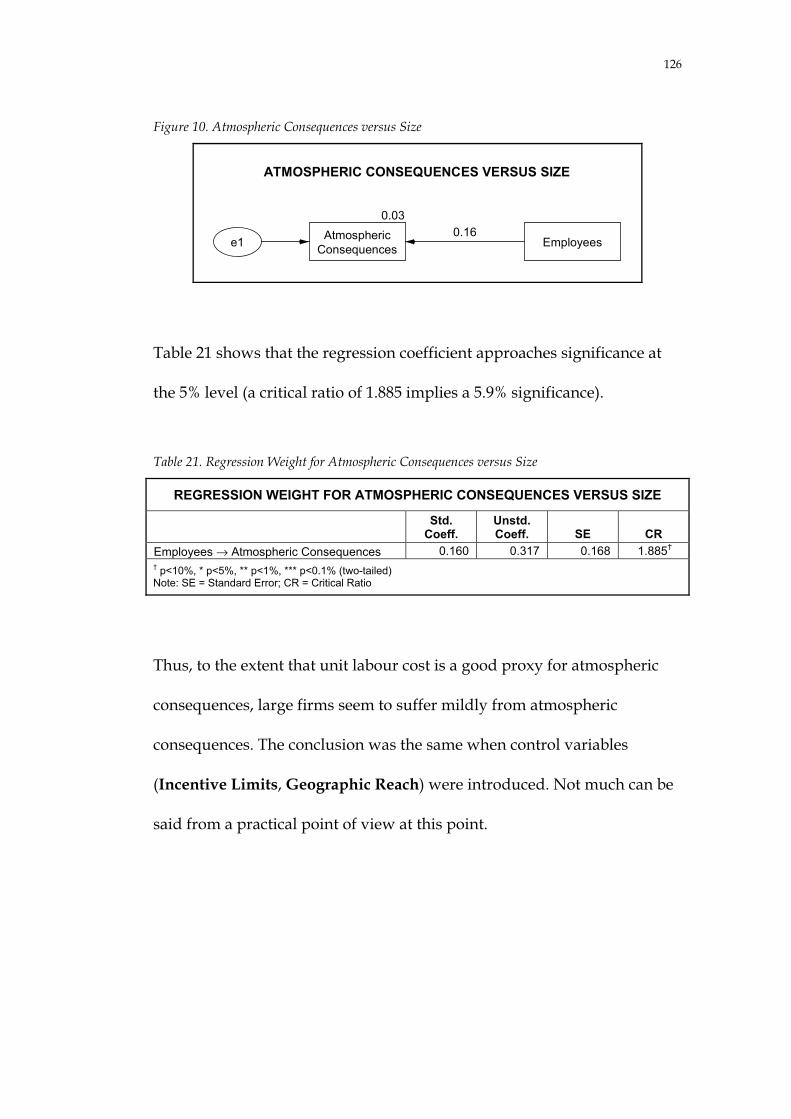
126
Figure 10. Atmospheric Consequences versus Size
ATMOSPHERIC CONSEQUENCES VERSUS SIZE
0.03Atmospheric
Consequencese1 Employees0.16
Table 21 shows that the regression coefficient approaches significance at
the 5% level (a critical ratio of 1.885 implies a 5.9% significance).
Table 21. Regression Weight for Atmospheric Consequences versus Size
REGRESSION WEIGHT FOR ATMOSPHERIC CONSEQUENCES VERSUS SIZE
Std. Coeff.
Unstd. Coeff. SE CR
Employees → Atmospheric Consequences 0.160 0.317 0.168 1.885†** † p<10%, * p<5%, ** p<1%, *** p<0.1% (two-tailed) Note: SE = Standard Error; CR = Critical Ratio
Thus, to the extent that unit labour cost is a good proxy for atmospheric
consequences, large firms seem to suffer mildly from atmospheric
consequences. The conclusion was the same when control variables
(Incentive Limits, Geographic Reach) were introduced. Not much can be
said from a practical point of view at this point.

127
6.1.1.2 Bureaucratic Insularity
Bureaucratic insularity was defined as executives’ propensity to become
increasingly isolated from market opportunities and from the lower levels
of the organisation as the firm grows and procedures and processes are
added to the organisational fabric. Indicators of bureaucratic insularity
could be the compensation of senior executives (because a prediction is
that executives will maximise their own gains rather than shareholder
gains), the age of the firm (because older firms should have built up more
of the insulating mechanisms), the tenure of the firm’s CEO and officers
(because high tenure should lead to higher insularity), or the share of free
cash flow being reinvested in the business with sub-standard (below cost-
of-capital) returns.
The choice was made to use the firm’s age (Company Age) and officers’
average tenure (Leadership Tenure) as indicators. Executive
compensation proved impossible to define in a meaningful way, as did
cash flow reinvestment, while CEO tenure was uncorrelated with other
variables.

128
Figure 11. Bureaucratic Insularity versus Size
BUREAUCRATIC INSULARITY VERSUS SIZE
0.13
LeadershipTenure
Employees
e1
0.10
CompanyAgee2
0.36
0.32
The path diagram in Figure 11 shows a strong relationship between
Leadership Tenure and Employees and between Company Age and
Employees. The regression weights (Table 22) are significant beyond the
0.1% level.
Table 22. Regression Weights for Bureaucratic Insularity versus Size
REGRESSION WEIGHTS FOR BUREAUCRATIC INSULARITY VERSUS SIZE
Std. Coeff.
Unstd. Coeff. SE CR
Employees → Leadership Tenure 0.364 0.695 0.139 4.992***Employees → Company Age 0.321 1.634 0.191 8.560****** p<0.1% (two-tailed)
The relationship between Employees and Company Age is in reality even
stronger, because almost all large firms are old, leading to
heteroscedasticity. This is evidenced by running the model with the large
firm sub-sample (392 largest firms). The critical ratio for Employees →

129
Company Age drops from 8.560 for all firms to 3.336 for large firms. In
practical terms, it is possible to conclude that bureaucratic insularity
increases with firm size and that the theoretical predictions are valid.
6.1.1.3 Incentive Limits
The third factor driving diseconomies of scale is incentive limits. As
discussed in Chapter 3, incentive limits are most serious in firms with
indivisible tasks such as product development, were the outcome of
activities is dependent on the collaboration of many individuals and the
contribution of each individual is hard to measure. Two indicators were
tested: (1) the research and development intensity, measured as R&D
expense divided by sales; and (2) general and administrative costs,
measured as SG&A expense less advertising expense, divided by sales.
The assumption behind the latter definition is that the bulk of general and
administrative activities are indivisible (e.g., general management tasks).
The two indicators have a fairly high correlation (52%). However, R&D%
has 489 observations, while SG&A% � Adv% only has 177 observations
and thus R&D% was chosen as the better indicator.
In the analysis of the relationship between incentive limits and size, the
approach is different from the one taken in the preceding two sections.
Large firms should try to avoid incentive limits. Consequently, one would

130
expect a negative regression coefficient for Employees → R&D%. This
should be especially true for firms in R&D-intense environments. The
three graphs in Figure 12 show this to be case. The first diagram shows the
regression for the whole sample of 784 firms. The second regression
includes only those firms with higher than average R&D intensity (245
firms). The third regression includes those firms with lower than average
R&D intensity (244 firms).30
Figure 12. Incentive Limits versus Size
INCENTIVE LIMITS VERSUS SIZEGroup: Total
Group: High R&D Intensity
Group: Low R&D Intensity
0.00Incentive
Limitse1 Employees0.00
0.01Incentive
Limitse1 Employees0.12
0.02Incentive
Limitse1 Employees�0.13
30 295 companies did not report their R&D expense.

131
The regression weights are reported in Table 23. The critical ratio for the
difference between the regression coefficient Employees → Incentive
Limits for the high R&D-intensity and the low R&D-intensity sub-samples
is 2.721. That is, the difference is significant at better than the 1% level and
one can conclude that firms in R&D-intense industries tend to be relatively
smaller. This lends support to the hypothesised impact of incentive limits
because large firms tend to avoid R&D-intense industries.
Table 23. Regression Weights for Incentive Limits versus Size
REGRESSION WEIGHTS FOR INCENTIVE LIMITS VERSUS SIZE
Std. Coeff.
Unstd. Coeff. SE CR
Total Sample: Employees → Incentive Limits 0.000 0.000 0.104 0.003***High R&D-Intensity Sub-Sample: Employees → Incentive Limits �0.127 �0.165 0.082 �2.000***Low R&D-Intensity Sub-Sample: Employees → Incentive Limits 0.118 0.169 0.091 1.860†**† p<10%, * p<5% (two-tailed)
The practical implication is that large firms suffer from incentive limits, in
line with the theoretical prediction.
6.1.1.4 Communication Distortion
The fourth and final factor contributing to diseconomies of scale is
communication distortion. Communication distortion can be defined as
the length of the communications process through the organisational

132
hierarchy, or as the time it takes for decisions to go from issue
identification to resolution. The first definition has usually been
operationalised with the number of hierarchical levels within the firm and
this is the definition used here as well. Unfortunately, it proved impossible
to operationalise the second definition.
A number of studies, including Child (1973), demonstrate that the number
of hierarchical levels increases logarithmically with the number of
employees. The current research reached the same conclusion by studying
the organisational structure of 386 firms within the total sample of 784
firms. They had an average of 7.9 hierarchical levels and a standard
deviation of 0.8 levels. No firm had more than 10 levels.
As expected, there is a strong dependency between number of employees
and the number of levels, as is shown in Figure 13.
Figure 13. Communication Distortion versus Size
COMMUNICATION DISTORTION VERSUS SIZE
0.75Communication
Distortione1 Employees0.87

133
The critical ratio is very high (Table 24). Additional regressions were run
with control variables such as organisational form (M-Form), but no such
control variable proved to be important.
Table 24. Regression Weight for Communication Distortion versus Size
REGRESSION WEIGHT FOR COMMUNICATION DISTORTION VERSUS SIZE
Std. Coeff.
Unstd. Coeff. SE CR
Employees → Communication Distortion 0.866 0.177 0.005 34.017****** p<0.1% (two-tailed)
The next section combines the variables discussed so far into an integrated
model for understanding diseconomies of scale, using latent variables in a
structural equation model.
6.1.1.5 Integrated Model for the Relationship between Diseconomies of Scale and Size
At this juncture, it appears likely that the four factors driving
diseconomies of scale according to transaction cost economics do indeed
increase with firm size. It is instructive to test this further by combining
atmospheric consequences, bureaucratic insularity, incentive limits and
communication distortion in one model to see how they collectively relate
to firm size. This is the first true structural equation model of the analysis
because two latent variables are introduced: Diseconomies of Scale and

134
Bureaucratic Insularity (so far, the analyses were run as standard
univariate linear regressions).
Figure 14 shows the structural equation model (partially31 corresponding
to sub-model a in Figure 9). Incentive Limits has Leadership Tenure and
Company Age as indicators. Diseconomies of Scale is a latent variable
constrained on the one hand by Employees, on the other hand by the four
factors driving diseconomies of scale. It should be noted that Incentive
Limits, which in the previous section was analysed differently than the
other three factors, has been modified in the model below. Because
incentive limits are most pronounced in R&D-intense industries, this had
to be taken into account. This was done by multiplying the original
Incentive Limits variable by a dummy factor of 1 for high R&D intensity
and 0 for low R&D intensity. (This is the only place in the thesis where this
alternative indicator for Incentive Limits is used.)
31 The other part of sub-model a is analysed in Section 6.1.2.

135
Figure 14. Diseconomies of Scale versus Size
DISECONOMIES OF SCALE VERSUS SIZE
0.04
IncentiveLimits
0.35
CompanyAge
0.41
LeadershipTenure
0.88
CommunicationDistortion
0.05
AtmosphericConsequences
0.85
Employees
0.21
e1
e2
e3
e4
e5
0.35
BureaucraticInsularity
0.64
0.59
e6
0.19
0.59
0.94
0.92
e7
Chi-square 33.213df 8Chi-square � df 4.152p 0.000
Diseconomiesof Scale
Diseconomiesof Scale
A matrix representation of the path diagram is provided in Figure 15.32 It
follows the notational conventions developed by Jöreskog and Sörbom
(see, e.g., Hair et al. 1998, 648–652).
32 The matrix equations are mathematically equivalent to the path diagram in Figure 14, but differ
in the arrangement of variables. The reason for this is that the path diagram does not make a clear distinction between the path diagram and the measurement model. The formal representation in the matrixes makes this distinction and it leads to a different layout of the path diagram. This layout increases the number of variables and makes the diagram unnecessarily complex, without changing the underlying equations. Thus, simplified path diagrams are used throughout the thesis.

136
Figure 15. Matrix Representation of Diseconomies of Scale versus Size
The path diagram in Figure 14 shows the standardised regression weights
and the squared multiple correlations. All the regression weights are
positive. This shows that the relationships have the hypothesised sign:
increasing size leads to increasing diseconomies of scale and all four
factors contribute to this increase. The squared multiple correlations vary
significantly though, from 0.04 to 0.88.
MATRIX REPRESENTATION OF DISECONOMIES OF SCALE VERSUS SIZE
Employees�1 =
emplX1 =
DistortionionCommunicat�LimitsIncentive�
InsularityicBureaucrat�esConsequenccAtmospheri�
ScaleofesDiseconomi�
5
4
3
2
1
=====
levelsYrdYageYtenureYulabourY
5
4
3
2
1
=====
������
�
�
������
�
�
+⋅
������
�
�
������
�
�
+⋅
������
�
�
������
�
�
=
������
�
�
������
�
�
3
1
1
51
41
31
21
1
11
5
4
3
2
1
�
�
�
����
�
�
�����
11 �X =
������
�
�
������
�
�
εε
+
������
�
�
������
�
�
������
�
�
������
�
�
=
������
�
�
������
�
�
3
2
5
4
3
2
1
Y33
Y23
5
4
3
2
1
�����
11
1
YYYYY
0� =
0� =

137
Table 25 shows that the critical ratios are significant at better than the 5%
level for all regression coefficients available (two coefficients were set to 1
to constrain the model). Furthermore, the model has a normed chi-square
of 4.152, indicating a good fit,33 and the normed fit index (NFI) is 0.995,
well above the threshold of 0.900.34
Table 25. Regression Weights for Diseconomies of Scale versus Size
REGRESSION WEIGHTS FOR DISECONOMIES OF SCALE VERSUS SIZE Std.
Coeff Unstd. Coeff. SE CR
Employees → Diseconomies of Scale 0.924 0.333 0.138 2.424***Diseconomies of Scale → Atmospheric Consequences 0.212 1 Diseconomies of Scale → Bureaucratic Insularity 0.589 1.981 0.901 2.197***Diseconomies of Scale → Incentive Limits 0.189 0.072 0.035 2.082***Diseconomies of Scale → Communication Distortion 0.938 0.534 0.220 2.424***Bureaucratic Insularity → Leadership Tenure 0.642 1 Bureaucratic Insularity → Company Age 0.594 2.491 0.526 4.733**** p<5%, *** p<0.1% (two-tailed)
The first hypothesis
H1: Bureaucratic failure, in the form of atmospheric consequences,
bureaucratic insularity, incentive limits and communication
distortion, increases with firm size
33 Excellent fit is defined as normed chi-square (chi-square � degrees of freedom) <2, good fit < 5,
and acceptable fit < 10. This is in line with Kelloway (1998, 28) and Hair et al. (1998, 623). 34 Recommended by Hair et al. (1998, 635–636).

138
is now expressed as: If �11>0, then H1 cannot be rejected. The standardised
coefficient is �11 = 0.92 and the significance is better than the 5% level,
supporting the hypothesis. The practical statistical significance is good
because of the strength of most of the relationships and the high
explanatory power of the analysis.
6.1.2 Economies of Scale
The literature survey was inconclusive regarding the effects of economies
of scale. The reasons were that while it is easy to conjecture that average
cost per unit of output falls with firm size, the scale effects may be
exhausted at fairly small firm sizes and they may apply to entire industries
rather than individual firms (because information travels fast and easily
between firms). Thus the choice of market or hierarchy may not matter.
This conclusion is somewhat at odds with the theory developed in this
research, as was noted in Section 3.2.2. It is therefore instructive to
incorporate economies of scale in the model to see whether there are any
scale effects.
Two indicators were tested. Both build on the assumption that economies
of scale exist when relative fixed costs are high. The chosen definition was
to take fixed and semi-fixed costs from the income statement and divide
these by total factor costs (including purchased goods and services). Factor

139
costs differ slightly from revenue because they are the sum of all inputs,
including cost of equity, regardless of if the sum of these inputs is larger or
smaller than revenue. This definition is equivalent to revenue less net
income plus cost of equity. By using factor costs rather than sales, spurious
business cycle effects due to yearly fluctuations in net income are
eliminated. The observed variable Fixed Cost% was consequently defined
as (SG&A + Depreciation + Interest) � Factor Costs. The definition
assumes that fixed costs are composed of more than the contribution from
fixed assets. Specifically, the level of SG&A expense (including R&D) is
not easily varied and can be considered fixed. The definition is equivalent
to Penrose’s definition ([1959] 1995, 89–95).
The second definition, which was discarded, was to use the classical
definition of fixed assets divided by sales. This definition had no statistical
significance, lending some credence to the argument made by Scherer and
Ross (1990) that if economies of scale exist, then they apply primarily to
bureaucratic costs (see also p. 64, above) and not to neoclassical
production costs.
Figure 16 shows the relationship between number of employees and
relative fixed cost. The significance of the regression coefficient is
negligible (with a critical ratio of 0.506), possibly because there are
countervailing forces at work, or because economies of scale do not exist.

140
The countervailing forces argument is that economies of scale on the one
hand lead large firms to be active in fixed cost-intense industries; on the
other hand, these very firms would realise the benefits of scale and thus
have lower relative fixed costs.
Figure 16. Fixed Cost versus Size: Total Sample
FIXED COST VERSUS SIZEGroup: Total
0.000.02
e1 Fixed Cost% Employees
With a similar logic as was employed in the case of incentive limits, it is
possible to test which of the two arguments is correct. If there are no
economies of scale then, two sub-samples consisting of (1) firms active in
high fixed-cost industries, and (2) firms active in low fixed-cost industries,
should not differ, while the opposite is true if economies of scale exist.
Figure 17 shows the path diagrams for these sub-samples with high fixed-
cost industries defined as those 377 firms with the highest fixed-cost ratio,
and low fixed-cost industries being the 376 remaining firms (with an
additional 31 firms having missing values). This categorisation is not
totally accurate because it would be better to use the fixed-cost intensity of
the entire industries to determine whether a firm is active in high or low
fixed-cost industries. Data were not available for this refinement.

141
Figure 17. Fixed Cost versus Size: High Fixed-Cost and Low Fixed-Cost Sub-Samples
FIXED COST VERSUS SIZEGroup: High Fixed Cost
Fixed Cost%e1 Employees
0.01�0.11
Group: Low Fixed Cost
Fixed Cost%e1 Employees
0.030.18
The regression coefficients differ for the two subsets and the critical ratio
for the difference is 3.472, implying significance better than the 0.1% level.
The regression weights for the total sample and the sub-samples are
shown in Table 26. The conclusion is that large firms have lower relative
fixed cost when operating in fixed cost-intense industries.
Table 26. Regression Weights for Fixed Cost versus Size
REGRESSION WEIGHTS FOR FIXED COST VERSUS SIZE
Std. Coeff.
Unstd. Coeff. SE CR
Total Sample: Employees → Fixed Cost% 0.018 0.004 0.008 0.506***High Fixed-Cost Sub-Sample: Employees → Fixed Cost% �0.107 �0.017 0.008 �2.096***Low Fixed-Cost Sub-Sample: Employees → Fixed Cost% 0.176 0.015 0.004 3.469**** p<5%, *** p<0.1% (two-tailed)

142
A problem with the approach taken above is that the two sub-samples
reduce the number of observations too much for the variables
Atmospheric Consequences and Leadership Tenure, which already in the
total sample have uncomfortably few observations. Rather than
performing the structural equation analysis on the two subsets defined
above, the variable Fixed Cost% was replaced with Economies of Scale.
Economies of Scale was constructed using the following logic: economies
of scale are large for those firms which simultaneously are active in high
fixed cost environments and have high (absolute) fixed costs. Thus, the
variable Economies of Scale multiplies the fixed cost ratio with the
absolute level of fixed cost (Economies of Scale = Fixed Cost% · Fixed
Cost). The relationship between economies of scale and firm size is shown
in Figure 18.
Figure 18. Economies of Scale versus Size
0.37
Economiesof Scalee1 Employees0.60
ECONOMIES OF SCALE VERSUS SIZE
Not surprisingly, the regression coefficient is highly significant at better
than the 0.1% level (Table 27).

143
Table 27. Regression Weight for Economies of Scale versus Size
REGRESSION WEIGHT FOR ECONOMIES OF SCALE VERSUS SIZE Std.
Coeff. Unstd. Coeff. SE CR
Employees → Economies of Scale 0.605 1.797 0.086 20.800****** p<0.1% (two-tailed)
The matrix representation in Figure 15 (p. 136, above) can now be
expanded to include economies of scale by adding �6 = �61�1 + �6 to
� = �x� + �� + � and Y6 = �6 to Y = y� + . This completes the matrix
representation of sub-model a.
At this point, the argument that economies of scale exist among large firms
(hypothesis two) cannot be rejected because � 61>0, with better than 0.1%
significance and
H2: Large firms exhibit economies of scale
is confirmed. The practical significance is also good because of the strength
of the relationship.
The analysis next continues with the structural equation models for sub-
model b.

144
6.2 SUB-MODEL B: RELATIONSHIP BETWEEN DISECONOMIES OF SCALE, ECONOMIES OF SCALE, MODERATING FACTORS AND FIRM PERFORMANCE
This section explores various aspects of sub-model b, which is the most
important part of the current research. It starts by testing the relationship
between a firm’s financial performance and the diseconomies-of-scale
factors (Section 6.2.1). It then adds economies of scale to the model to test
whether they do influence firm performance positively, as predicted by
the theoretical framework (Section 6.2.2). Next, the moderating factors (M-
form organisation and high asset specificity) are included in the sub-
model (Section 6.2.3). The final section (6.2.4) discusses the full sub-model
and introduces alternative specifications to achieve parsimony. The
statistical findings are shown to be congruent with the TCE framework.
6.2.1 Diseconomies of Scale and Their Impact on Firm Performance
Similar to the treatment of sub-model a in Section 6.1.1, this section first
discusses each of the diseconomies-of-scale factors individually, and then
combines them in an integrated model to test the relationship between
diseconomies of scale and firm performance. The individual analyses
should be seen as initial indications of dependencies and will guide the
design of the integrated model. Four sections (6.2.1.1–6.2.1.4) discuss
atmospheric consequences, bureaucratic insularity, incentive limits and

145
communication distortion, respectively. The fifth section (6.2.1.5) tests the
integrated model.
6.2.1.1 Atmospheric Consequences
Figure 19 shows that Atmospheric Consequences have a negative
influence on Growth and have no material influence on Profitability.
Atmospheric Consequences explains 11% of the variance in Growth.
Figure 19. Firm Performance versus Atmospheric Consequences
FIRM PERFORMANCE VERSUS ATMOSPHERIC CONSEQUENCES
0.11
Growth
Atmospheric Consequences
e1
0.00
Profitabilitye2
�0.34
�0.07
Table 28 shows that the regression coefficient for Atmospheric
Consequences → Growth is significant beyond the 0.1% level. The results
were similar for two sub-samples; the largest 392 firms and the smallest
392 firms (the critical ratio for the differences were 0.129 for Atmospheric

146
Consequences → Growth and �0.570 for Atmospheric Consequences →
Profitability).
Table 28. Regression Weights for Firm Performance versus Atmospheric Consequences
REGRESSION WEIGHTS FOR FIRM PERFORMANCE VERSUS ATMOSPHERIC CONSEQUENCES
Std. Coeff.
Unstd. Coeff. SE CR
Atmospheric Consequences → Growth �0.337 �0.139 0.030 �4.691***Atmospheric Consequences → Profitability �0.069 �0.040 0.040 �1.010****** p<0.1% (two-tailed)
The practical implication is that atmospheric consequences influence
growth negatively and may have the same influence on profitability.
6.2.1.2 Bureaucratic Insularity
The discussion in Section 6.1.1.2 showed that bureaucratic insularity can
be indicated by leadership tenure and firm age. The path diagram in
Figure 20 shows that both these indicators exhibit strong negative
influences on growth and that tenure also influences profitability
negatively. However, firm age has a positive influence on profitability. It
can be hypothesised that this is because of survivor bias, as discussed
earlier (see pp. 65–66, above). That is, the firms in the sample are by
definition survivors and thus can be expected to show higher profitability
than non-surviving firms. This implies that firms that have survived over

147
a long time period should be more profitable than young firms because
younger firms (usually in younger industries) include a more
heterogeneous mix of performers. This hypothesis is tested in
Section 6.2.1.5, where the larger, integrated model is analysed using latent
variables.
Figure 20. Firm Performance versus Bureaucratic Insularity
FIRM PERFORMANCE VERSUS BUREAUCRATIC INSULARITY
0.23
Growth
�0.39
e1
0.03
Profitability0.19
e2
�0.18
�0.11
CompanyAge
LeadershipTenure
At this point, the analysis suggests support for Penrose’s ([1959] 1995, 261–
263) assertion that diseconomies of scale are mainly related to difficulties
of growth. Bureaucratic Insularity (indicated by Leadership Tenure and
Company Age) explains 23% of the variance in Growth, but only 3% of
the variance in Profitability. For Growth, the regression weights are
significant at better than the 5% level (Table 29).
Note: The complete diagram, with correlations, is found in Figure C.1 (Appendix C)

148
Table 29. Regression Weights for Firm Performance versus Bureaucratic Insularity
REGRESSION WEIGHTS FOR FIRM PERFORMANCE VERSUS BUREAUCRATIC INSULARITY
Std. Coeff.
Unstd. Coeff. SE CR
Leadership Tenure → Growth �0.177 �0.070 0.029 �2.431***Leadership Tenure → Profitability �0.114 �0.063 0.044 �1.445***Company Age → Growth �0.386 �0.056 0.007 �8.498***Company Age → Profitability 0.190 0.039 0.010 3.832**** p<5%, *** p<0.1% (two-tailed)
6.2.1.3 Incentive Limits
Do incentive limits have an impact on a firm’s performance (indicated as
before through Growth and Profitability)? In this analysis, Company Age
was introduced as a control variable because older firms tend to be active
in mature industries. Figure 21 indicates a modest impact.
Figure 21. Firm Performance versus Incentive Limits
FIRM PERFORMANCE VERSUS INCENTIVE LIMITS
0.20
Growthe1
0.03
Profitabilitye2
�0.01
�0.10
�0.46
0.12
IncentiveLimits
CompanyAge
Note: The complete diagram, with correlations, is found in Figure C.2 (Appendix C)

149
The regression shows a negative impact of incentive limits on profitability
(at better than the 5% significance level). The impact on growth is
negligible (Table 30).
Table 30. Regression Weights for Firm Performance versus Incentive Limits
REGRESSION WEIGHTS FOR FIRM PERFORMANCE VERSUS INCENTIVE LIMITS Std.
Coeff. Unstd. Coeff. SE CR
Incentive Limits → Growth �0.010 �0.003 0.014 �0.235***Incentive Limits → Profitability �0.102 �0.047 0.021 �2.193***Company Age → Growth �0.455 �0.066 0.005 �12.195***Company Age → Profitability 0.121 0.025 0.008 2.962**** p<5%, ** p<1%, *** p<0.1% (two-tailed)
There should be a difference between the high R&D-intensity and the low-
R&D% intensity sub-samples. The R&D% → Profitability standardised
coefficient is �0.134 for the high R&D-intensity sub-sample and 0.130 for
the low R&D-intensity sub-sample, in support of the theory. The critical
ratio for this difference is 2.853 and the significance is better than the 1%
level. There is considerable support for the hypothesis (H3c), that incentive
limits affect performance by having a negative impact on profitability.
6.2.1.4 Communication Distortion
In isolation, communication distortion does not have a significant impact
on firm performance as is evidenced by the regression in Figure 22. Less
than 2% of the variance in growth and profitability are accounted for.

150
Figure 22. Firm Performance versus Communication Distortion
FIRM PERFORMANCE VERSUS COMMUNICATION DISTORTION
0.02
Growth
CommunicationDistortion
e1
0.01
Profitabilitye2
�0.14
0.07
Table 31 shows that only the negative impact on growth is statistically
significant (at better than the 1% level), but it is hard to draw any practical
conclusions at this stage.
Table 31. Regression Weights for Firm Performance versus Communication Distortion
REGRESSION WEIGHTS FOR FIRM PERFORMANCE VERSUS COMMUNICATION DISTORTION
Std. Coeff.
Unstd. Coeff. SE CR
Communication Distortion → Growth *�0.136 �0.484 0.180 �2.688***Communication Distortion → Profitability 0.075 0.372 0.251 1.481***** p<1% (two-tailed)
The next section (6.2.1.5) combines the variables into an integrated model
for understanding the relationship between firm performance and
diseconomies of scale.

151
6.2.1.5 Integrated Model for the Relationship between Firm Performance and Diseconomies of Scale
It is now time to put together an integrated diseconomies-of-scale model,
bearing in mind economies of scale and the moderating factors (M-form
organisation and asset specificity) have not yet been introduced, nor has
survivor bias. The path diagram in Figure 23 shows the design which tests
the third hypothesis and its four sub-hypotheses. The latent variable
Bureaucratic Insularity is again used and is indicated by Leadership
Tenure and Company Age.

152
Figure 23. Firm Performance versus Diseconomies of Scale: Not Adjusted for Survivor Bias
FIRM PERFORMANCE VERSUS DISECONOMIES OF SCALENot adjusted for Survivor Bias
Chi-square 16.490df 4Chi-square � df 4.123p 0.002
Growth
Profitability
0.08
�0.01
0.54
0.25
�0.090.26
�0.21�0.18
0.11
0.01
�0.630.430.74
IncentiveLimits
AtmosphericConsequences
e1
e2
BureaucraticInsularity
CommunicationDistortion
0.50
LeadershipTenure
e4CompanyAge
e3
The model has a chi-square of 16.490 and 4 degrees of freedom, leading to
a normed chi-square of 4.123 (a good fit). The normed fit index (NFI) is
0.997, well beyond any reasonable requirement, and the parsimonious fit
index (PFI) is 0.143.
Note: The complete diagram, with correlations, is found in Figure C.3 (Appendix C)

153
Table 32 shows the regression weights with standard errors and critical
ratios.
Table 32. Regression Weights for Firm Performance versus Diseconomies of Scale: Not Adjusted for Survivor Bias
REGRESSION WEIGHTS FOR FIRM PERFORMANCE VERSUS DISECONOMIES OF SCALE
Not Adjusted for Survivor Bias Std.
Coeff. Unstd. Coeff. SE CR
Atmospheric Consequences → Growth �0.179 �0.071 0.044 �1.644†** Atmospheric Consequences → Profitability �0.210 �0.118 0.056 �2.117***Bureaucratic Insularity → Growth �0.626 �0.123 0.042 �2.947***Bureaucratic Insularity → Profitability 0.261 0.072 0.035 2.072***Bureaucratic Insularity → Leadership Tenure 0.502 0.249 0.049 5.037***Bureaucratic Insularity → Company Age 0.737 1.000 Incentive Limits → Growth �0.087 �0.028 0.034 �0.824***Incentive Limits → Profitability �0.009 �0.004 0.035 �0.114***Communication Distortion → Growth 0.113 0.399 0.317 1.259***Communication Distortion → Profitability 0.008 0.042 0.344 0.121* *† p<10%, * p<5%, ** p<1%, *** p<0.1% (two-tailed)
Bureaucratic insularity has a strong negative impact on growth
(Bureaucratic Insularity → Growth = �0.63) and is significant at better
than the 1% level (critical ratio = �2.947), while it has a significant positive
impact on profitability (Bureaucratic Insularity → Profitability = 0.26)
before the adjustment for survivor bias. Communication distortion has a
non-significant (less than 10% level) positive impact on both growth and
profitability (critical ratio = 1.259 and 0.121, respectively). Atmospheric
consequences have a negative impact on both growth (Atmospheric
Consequences → Growth = �0.18) and profitability (Atmospheric
Consequences → Profitability = �0.21) with significance better than the

154
10% level (critical ratios �1.650 and �2.117 respectively). It should be
remembered that Atmospheric Consequences has few (146) observations.
Finally, incentive limits have a negative impact on profitability with a low
significance (critical ratio = �0.824) and there is a negative, non-significant,
impact on growth (critical ratio = �0.114). The regression coefficients thus
are either directionally in line with the hypothesis for each factor, or they
are insignificant (except for Bureaucratic Insularity → Profitability).35 In
no case was there a statistically significant contradiction of the hypothesis.
Finally, the squared multiple correlation is a high 0.425 for Growth and a
low 0.077 for Profitability.
A second path diagram was constructed to take survivor bias into account.
This was done by introducing a link between Company Age and
Profitability, as was explained in Section 6.2.1.2. This model is less
parsimonious (PFI = 0.107) and has a slightly higher normed chi-square
(4.670) than the non-adjusted model. Yet it is probably a more realistic
representation of the underlying theory and hypotheses and it will be used
in the later analyses.
35 The correlations between the diseconomies of scale factors also have the expected signs (see
Appendix C).

155
Figure 24. Firm Performance versus Diseconomies of Scale: Adjusted for Survivor Bias
FIRM PERFORMANCE VERSUS DISECONOMIES OF SCALEAdjusted for Survivor Bias
Chi-square 14.011df 3Chi-square � df 4.670p 0.003
Growth
Profitability
0.09
�0.17
0.51
0.28
�0.12�0.33
�0.06�0.15
0.14
0.14
0.32
�0.670.450.71
IncentiveLimits
AtmosphericConsequences
e1
e2
BureaucraticInsularity
CommunicationDistortion
0.53
CompanyAge e4
LeadershipTenure e3
The regression coefficients, standard errors and critical ratios are reported
in Table 33. Without repeating the discussion from the previous path
diagram, it should be noted that bureaucratic insularity now has the
hypothesised (but non-significant) negative impact on profitability. The
survivor bias (Company Age → Profitability = 0.32) has a positive
Note: The complete diagram, with correlations, is found in Figure C.4 (Appendix C)
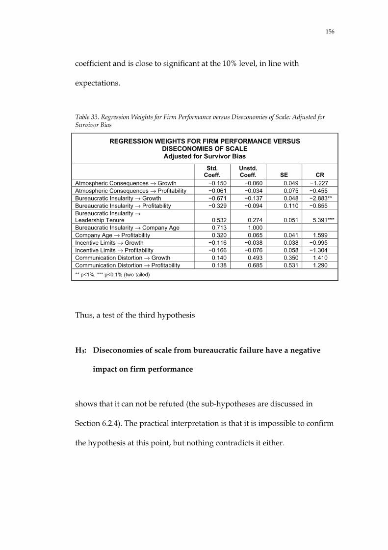
156
coefficient and is close to significant at the 10% level, in line with
expectations.
Table 33. Regression Weights for Firm Performance versus Diseconomies of Scale: Adjusted for Survivor Bias
REGRESSION WEIGHTS FOR FIRM PERFORMANCE VERSUS DISECONOMIES OF SCALE Adjusted for Survivor Bias
Std. Coeff.
Unstd. Coeff. SE CR
Atmospheric Consequences → Growth �0.150 �0.060 0.049 �1.227* *Atmospheric Consequences → Profitability �0.061 �0.034 0.075 �0.455***Bureaucratic Insularity → Growth �0.671 �0.137 0.048 �2.883***Bureaucratic Insularity → Profitability �0.329 �0.094 0.110 �0.855***Bureaucratic Insularity → Leadership Tenure 0.532 0.274 0.051 5.391***Bureaucratic Insularity → Company Age 0.713 1.000 Company Age → Profitability 0.320 0.065 0.041 1.599***Incentive Limits → Growth �0.116 �0.038 0.038 �0.995***Incentive Limits → Profitability �0.166 �0.076 0.058 �1.304***Communication Distortion → Growth 0.140 0.493 0.350 1.410***Communication Distortion → Profitability 0.138 0.685 0.531 1.290***** p<1%, *** p<0.1% (two-tailed)
Thus, a test of the third hypothesis
H3: Diseconomies of scale from bureaucratic failure have a negative
impact on firm performance
shows that it can not be refuted (the sub-hypotheses are discussed in
Section 6.2.4). The practical interpretation is that it is impossible to confirm
the hypothesis at this point, but nothing contradicts it either.

157
6.2.2 Economies of Scale
The next step is to study the impact of economies of scale on profitability
(there is no hypothesised impact on the other indicator of firm
performance: growth). This was done by adding diseconomies of scale to
the path diagram containing diseconomies of scale. The path diagram in
Figure 25 shows the results. Chi-square is 8.995 and with 5 degrees of
freedom the normed chi-square ratio is 1.799, indicating an excellent fit
(p = 0.109). The normed fit index (NFI) is an excellent 0.999 and the
parsimonious fit index (PFI) is 0.139, which is slightly better than for the
previous model (Figure 24) which only incorporated diseconomies of
scale. The squared multiple correlation is 0.44 for Growth and 0.12 for
Profitability.

158
Figure 25. Firm Performance versus Diseconomies of Scale and Economies of Scale
FIRM PERFORMANCE VERSUS DISECONOMIES OF SCALEAND ECONOMIES OF SCALE
Growth
Chi-square 8.995df 5Chi-square � df 1.799p 0.109
0.12
�0.25
0.49
0.28
�0.12�0.32
�0.14�0.08
0.15
�0.01
0.30
0.27
�0.720.440.70
AtmosphericConsequences
e1
e2
BureaucraticInsularity
Economiesof Scale
CommunicationDistortion
0.53
IncentiveLimits
CompanyAge e4
LeadershipTenure e3
Profitability
Table 34 reports the regression coefficients. All coefficients have the
hypothesised sign except for Communication Distortion → Growth. This
aberration could be because the theory does not specify any relationship
between economies of scale and growth—only between economies of scale
and profitability. If such an atheoretical relationship exists, then
communication distortion’s positive impact on growth could be due to the
Note: The complete diagram, with correlations, is found in Figure C.5 (Appendix C)

159
unobserved positive relationship between economies of scale and growth.
This was tested separately. The standardised regression coefficient was
0.00 for Economies of Scale → Growth and it remained at 0.15 for
Communication Distortion → Growth with this respecification of the
model. Fit measures deteriorated slightly. Thus, the structural equation
model in Figure 25 appears to be correctly specified because economies of
scale do not influence growth, as hypothesised.
The regression coefficients mostly do not have high significance. The
exceptions are Bureaucratic Insularity → Growth and Bureaucratic
Insularity → Leadership Tenure which are significant at better than the
0.1% level, Economies of Scale → Profitability at better than 1% and
Incentive Limits → Profitability and Company Age → Profitability at
better than 10%. All other coefficients have the predicted sign except for
Communication Distortion → Growth.
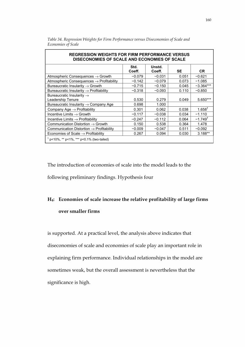
160
Table 34. Regression Weights for Firm Performance versus Diseconomies of Scale and Economies of Scale
REGRESSION WEIGHTS FOR FIRM PERFORMANCE VERSUS DISECONOMIES OF SCALE AND ECONOMIES OF SCALE
Std. Coeff.
Unstd. Coeff. SE CR
Atmospheric Consequences → Growth �0.079 �0.031 0.051 �0.621***Atmospheric Consequences → Profitability �0.142 �0.079 0.073 �1.085***Bureaucratic Insularity → Growth �0.715 �0.150 0.045 �3.364***Bureaucratic Insularity → Profitability �0.318 �0.093 0.110 �0.850***Bureaucratic Insularity → Leadership Tenure 0.530 0.279 0.049 5.650***Bureaucratic Insularity → Company Age 0.698 1.000 Company Age → Profitability 0.301 0.062 0.038 1.658†** Incentive Limits → Growth �0.117 �0.038 0.034 �1.110***Incentive Limits → Profitability �0.247 �0.112 0.064 �1.749†** Communication Distortion → Growth 0.150 0.538 0.364 1.478***Communication Distortion → Profitability �0.009 �0.047 0.511 �0.092***Economies of Scale → Profitability 0.267 0.094 0.030 3.188***† p<10%, ** p<1%, *** p<0.1% (two-tailed)
The introduction of economies of scale into the model leads to the
following preliminary findings. Hypothesis four
H4: Economies of scale increase the relative profitability of large firms
over smaller firms
is supported. At a practical level, the analysis above indicates that
diseconomies of scale and economies of scale play an important role in
explaining firm performance. Individual relationships in the model are
sometimes weak, but the overall assessment is nevertheless that the
significance is high.

161
An interpretation of the statistical results is that firms are able to maintain
specific knowledge internally and that the flow of ideas and methods in
external markets is not efficient enough to make economies of scale
available to all industry participants. A further test of this was made by
splitting the sample by the age of firms. The assumption was that older
firms, active in older, well-structured industries where information
presumably flows efficiently, would not benefit from economies of scale.
Younger firms, active in less mature industries, would, if they are larger
than their competitors, reap the benefits because knowledge should be
easier to keep proprietary to the firm. If this was true, then Riordan and
Williamson’s theoretical prediction (1985) that economies of scale affect
firm performance could be questioned. A comparison of the sub-samples
indicates that this is not the case. The two sub-samples have almost
identical regression coefficients for Economies of Scale → Profitability
(0.291 for the old sub-sample, 0.292 for the young sub-sample) and the
critical ratio for the difference is a negligible �0.115.
The next step is to incorporate the potential effects of moderating factors
into the model. While additional insights are gained from this, it should
also be noted that the model becomes less statistically robust as variables
are added—especially because some of the variables are non-normal—and

162
the model fit will deteriorate. At the same time though, the practical
significance increases.
6.2.3 Moderating Factors
At this stage the final two variables are introduced into the model: the
moderating factors organisational form and asset specificity.
6.2.3.1 M-Form Organisation
Williamson (1970, 120–139) argued that the large multidivisional firm (M-
form) on average outperforms the large unitary firm (U-form).
Williamson’s definition of M-form was (pp. 120–121):
1. The responsibility for operating decisions is assigned to…operating divisions or quasifirms.
2. The elite staff attached to the general office performs both advisory and auditing functions…
3. The general office is principally concerned with strategic decisions…
4. …separation of the general office from operations…
5. The resulting structure displays both rationality and synergy…the whole is greater than the sum of the parts.
This definition can be operationalised with two indicators. The first
describes the ability of a firm to effectively to divide the tasks performed

163
by senior executives and their staffs, as well as the division of
responsibility between the board of directors and executive management
(pp. 138–139)—what today often is referred to as governance.36 The second
variable measures whether the organisational structure is multidivisional
or functional, or somewhere in between.
The governance indicator was operationalised as Governance, based on
CalPERS’s definitions (1999).37 CalPERS evaluates corporate governance
using financial results (three-year shareholder returns and EVA) and a
corporate governance screening procedure which assesses the quality of
governance. For the current purposes the governance screen is of interest,
so that co-linearity with the dependent variables is avoided. The screen
uses 25 criteria divided into four main categories: “Board
Composition/Structure”, “Director Compensation/Stock Holdings”,
“Management” and “Anti-Takeover Devices”.
The data were taken from three sources: (1) Business Week’s annual survey
of corporate governance (Byrne 2000). Business Week measures six
attributes of governance and of these, four were used in Governance
because they correspond reasonably well to the CalPERS criteria, while
36 A fuller treatment of this dual relationship is found in Bolton and Scharfstein (1998). 37 CalPERS (California Public Employees’ Retirement System) is arguably the world’s leading
authority on governance issues.

164
two (relating to the quality of the board members) where excluded. (2) The
compilation of governance data for 1,500 companies published by the
Investor Responsibility Research Center (IRRC 1999).38 (3) Fortune’s annual
ranking of America’s most admired companies (Colvin 2000) in which
three variables (of eight) relate to CalPERS’s governance criteria. The three
sources were merged into a single index. No attempt was made
independently to validate the definitions and underlying research, except
for using this researcher’s general understanding of the quality of
governance at those firms surveyed. This crude test corroborated the data.
The organisational structure indicator was operationalised as
Divisionalisation. The indicator is ordinal with 2 representing a clean,
multidivisional structure, 1 representing a mixture of multidivisional and
unitary structures and 0 representing unitary structures. The classification
was done by this researcher using annual reports, corporate web sites,
company organisation charts and 10-Ks. The data collection approach was
similar to Rumelt’s (1974, 43), with three factors influencing the judgments
made: titles of senior executives, descriptions of large operating units and
the reporting or lack of reporting of operating unit financials. For example,
if senior executives at headquarters have titles such as Senior Vice
President of Business Development and similar staff descriptions, while
38 CalPERS subcontracts the governance screening to IRRC.
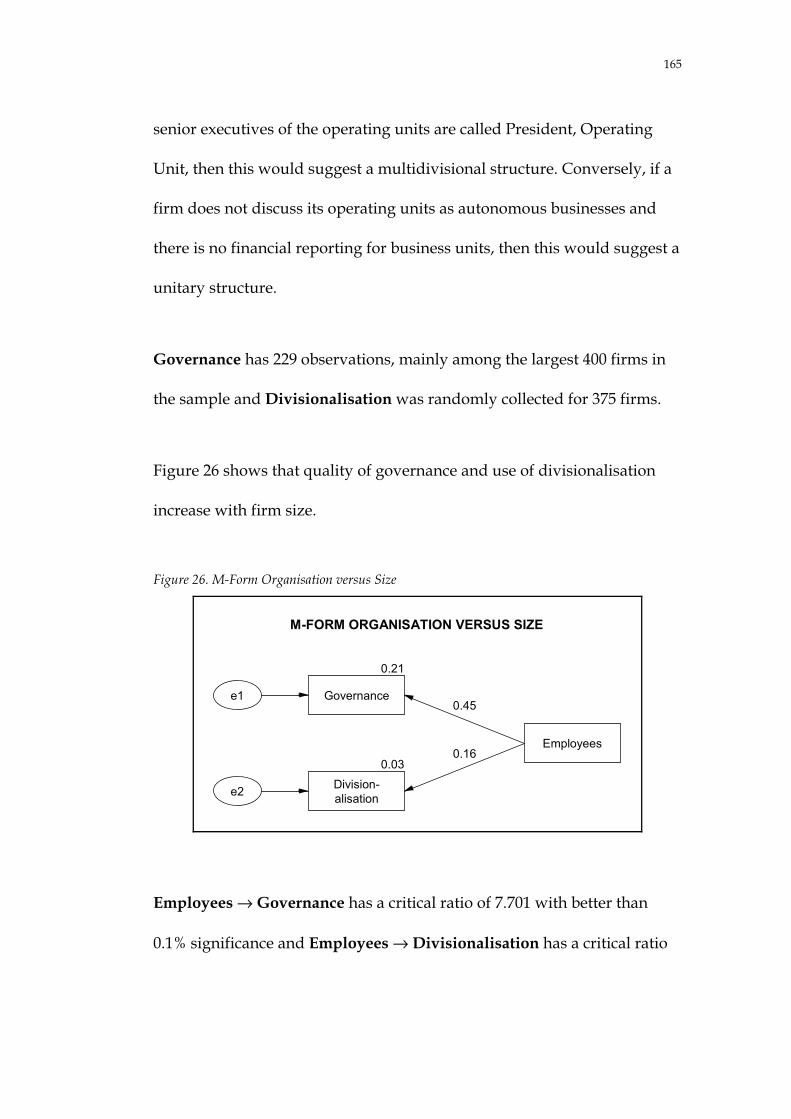
165
senior executives of the operating units are called President, Operating
Unit, then this would suggest a multidivisional structure. Conversely, if a
firm does not discuss its operating units as autonomous businesses and
there is no financial reporting for business units, then this would suggest a
unitary structure.
Governance has 229 observations, mainly among the largest 400 firms in
the sample and Divisionalisation was randomly collected for 375 firms.
Figure 26 shows that quality of governance and use of divisionalisation
increase with firm size.
Figure 26. M-Form Organisation versus Size
M-FORM ORGANISATION VERSUS SIZE
0.21
Governance
Employees
e1
0.03
Division-alisatione2
0.45
0.16
Employees → Governance has a critical ratio of 7.701 with better than
0.1% significance and Employees → Divisionalisation has a critical ratio

166
of 3.230, approaching better than 0.1% significance (Table 35). It should be
remembered that Divisionalisation is an ordinal variable and Amos treats
it as continuous. Results would perhaps be more accurate if polyserial
correlations were used and the squared multiple correlation would then
increase somewhat, while the significance would be better than the 0.1%
level.39
Table 35. Regression Weights for Firm Performance versus Diseconomies of Scale, Economies of Scale and M-form Organisation
REGRESSION WEIGHTS FOR FIRM PERFORMANCE VERSUS DISECONOMIES OF SCALE, ECONOMIES OF SCALE AND M-FORM ORGANISATION
Std. Coeff.
Unstd. Coeff. SE CR
Employees → Governance 0.454 0.545 0.071 7.701***Employees → Divisionalisation 0.165 0.257 0.080 3.230***** p<1%, *** p<0.1% (two-tailed)
Turning to the prediction that M-form organisation improves firm
performance, the latent variable M-Form was introduced into the sub-
model b path diagram together with the indicators Governance and
Divisionalisation. The results are shown in Figure 27. M-form
organisation has a significant, positive impact on both growth and
profitability with most of the impact emanating from governance. This is
not surprising because, as was discussed in the literature survey (p. 67,
39 This analysis was performed using LISREL which allows for polyserial correlation analysis. The
regression coefficient increased to 0.20 from 0.16 and the squared multiple correlation to 0.049 from 0.025. However, the use of polyserial correlations assumes that the underlying distribution of the indicator is normal, which may not be the case here (see also discussion in Section 5.1.2.3).

167
above), the positive impact of divisionalisation was exploited more than 25
years ago.
Figure 27. Firm Performance versus Diseconomies of Scale, Economies of Scale and M-Form Organisation
FIRM PERFORMANCE VERSUS DISECONOMIES OF SCALE,ECONOMIES OF SCALE AND M-FORM ORGANISATION
e9
0.29
�0.31
0.48
0.29
�0.12�0.43
�0.09�0.08
0.63
Governance
0.01Division-alisation
0.79 0.09
�0.06
0.36
0.21
0.38
0.28
�0.71
Chi-square 75.618df 17Chi-square � df 4.448p 0.000
e8
Governance
0.500.70
AtmosphericConsequences
e1
e2
Economiesof Scale
M-Form
0.53
LeadershipTenure e3
e4
BureaucraticInsularity
Growth
IncentiveLimits
CommunicationDistortion
CompanyAge
Profitability
0.11
Note: The complete diagram, with correlations, is found in Figure C.6 (Appendix C)

168
Table 36 shows similar results as in earlier analyses, with all coefficients
(except for Communication Distortion → Growth) having the predicted
sign and with critical ratios ranging from highly significant to non-
significant. The standardised regression coefficients are fairly large for M-
Form → Growth (0.21) and M-Form → Profitability (0.38), but the
statistical significance is low. The practical significance is good though,
because a good part of the variance in firm performance is explained and
all relationships (with one exception) support the underlying theoretical
framework.
Table 36. Regression Weights for Firm Performance versus Diseconomies of Scale, Economies of Scale and M-Form Organisation
REGRESSION WEIGHTS FOR FIRM PERFORMANCE VERSUS DISECONOMIES OF SCALE, ECONOMIES OF SCALE AND M-FORM ORGANISATION
Std. Coeff.
Unstd. Coeff. SE CR
Atmospheric Consequences → Growth �0.080 �0.032 0.048 �0.669***Atmospheric Consequences → Profitability �0.085 �0.048 0.071 �0.674***Bureaucratic Insularity → Growth �0.706 �0.149 0.044 �3.412***Bureaucratic Insularity → Profitability �0.433 �0.127 0.106 �1.192***Bureaucratic Insularity → Leadership Tenure 0.534 0.282 0.049 5.709***Bureaucratic Insularity → Company Age 0.696 1.000 Company Age → Profitability 0.355 0.073 0.038 1.934†** Incentive Limits → Growth �0.124 �0.040 0.032 �1.253***Incentive Limits → Profitability �0.312 �0.142 0.062 �2.296***Communication Distortion → Growth 0.108 0.395 0.407 0.971***Communication Distortion → Profitability �0.062 �0.316 0.746 �0.423***Economies of Scale → Profitability 0.284 0.100 0.035 2.835***M-Form → Growth 0.207 0.170 0.228 0.747***M-Form → Profitability 0.385 0.439 0.578 0.760***M-Form → Governance 0.792 1.000 M-Form → Divisionalisation 0.091 0.156 0.184 0.852***† p<10%, * p<5%, ** p<1%, *** p<0.1% (two-tailed)

169
6.2.3.2 High Internal Asset Specificity
The last variable to be introduced is asset specificity. As was discussed in
the literature survey (Chapter 3), firms can, according to transaction cost
economics, moderate diseconomies of scale by increasing their internal
asset specificity. Asset specificity was measured in three ways: product
breadth, geographic reach and vertical depth. Each of these was
operationalised.
Product breadth was defined in several ways. In the end, Rumelt’s
(1974, 14–15) specialisation ratio was used because it is commonly
accepted (Ramanujam and Varadarajan 1989, 539) and it minimises
information loss. It also has the benefit of not being based on this
researcher’s judgement. To avoid confusion, product breadth was
operationalised as a diversification ratio equal to 1 � specialisation ratio
(so that the indicator increases when product breadth increases). The
specialisation ratio is defined as SR = (sales from the largest business unit)
� (total firm sales). Alternative measures (available at http://canback.com/
henley.htm in the file Asset Specificity.xls) are (1) number of business
segments the firm is active in; (2) number of SICs the firm is active in;
(3) Rumelt’s relatedness ratio (pp. 15–16): RR = (sales from the largest
business unit plus other business units with related activities) � (total firm
sales); (4) Rumelt’s five category classification of firms into single,

170
dominant-unrelated, dominant, related and unrelated businesses (p. 31);
and (5) a Herfindahl index of corporate diversity. Measures 1, 2 and 4 are
based on categorical data and are as such less rich on information than the
other measures. Measures 3 and 5 are continuous but less accurate than
the specialisation ratio for the current purpose.
Geographic reach was measured as the per cent of sales derived from
foreign countries. No other measures were available from Compustat or
other sources and the measure appears to be logical. Sullivan (1994), in an
overview of how geographic reach is measured, showed that all 17 studies
in his sample used this measure: “glaring in its consistency is the
inevitable use of foreign sales as a percentage of total sales (FSTS) as the
sole estimator” (pp. 327, 330).
Vertical depth was more problematic to define, however. Vertical
integration has been studied empirically many times (Shelanski and Klein
1995). The best measure (described by D’Aveni and Ravenscraft (1994)) is
arguably to quantify the amount of internal forward or backward transfers
by line of business. Unfortunately such data were not available for
individual firms. Another measure often used is value added (factor costs
other than purchased goods) divided by sales. This measure has been
criticised because it is sensitive to current year profitability; spuriously
high or low profitability increases or decreases vertical integration (Levy

171
1981, 86). A modification to this ratio is to adjust the nominator by using
cost of equity rather than net income and the denominator by using factor
costs, as defined earlier (i.e., VI% = Value Added � Factor Costs). Even
with this adjustment the definition is open to criticism.40 For example,
large US petrochemical companies are among the most vertically
integrated firms in the world, ranging in activities from exploration, to
production, to refining, to retailing. Their vertical integration ratios, with
this definition, are among the lowest, however (e.g., ExxonMobil has a
vertical integration of 19.1%, against 41.3% for the total sample).
Instead, the vertical integration variable was based on a qualitative
assessment by the researcher, similar to Armour and Teece’s (1980, 472)
and Harrigan’s (1986, 538–540) methodologies. The 784 firms were
classified based on their degree of vertical integration with Vertical Depth
equal to 2 for firms with very high vertical integration (13 firms), 1 for
highly integrated firms (145 firms) and 0 for firms with normal or low
integration (512 firms).41 No judgement was passed on 114 firms.
Vertically integrated firms were mainly found among resource-based
companies and among aerospace contractors. The data are available in the
file Asset Specificity.xls at http://canback.com/henley.htm. The polyserial
40 Furthermore, there were only 146 observations of the vertical integration ratio in the sample. 41 The underlying actual distribution of Vertical Depth is most likely normal, because VI% is
normally distributed, and Vertical Depth should have the same distributional characteristics (see discussion in Section 5.1.2.3).

172
correlation between Vertical Depth and VI% was �0.418, which seems to
confirm the criticism of the use of the value added-to-factor costs ratio.
Figure 28 shows the relationship between product breadth, geographic
reach, vertical depth and firm size.
Figure 28. Asset Specificity versus Size
ASSET SPECIFICITY VERSUS SIZE
0.08ProductBreadthe2 Employees0.29
0.08Geographic
Reache1
0.01VerticalDepthe3
0.27
0.10
Large size on average leads to less asset specificity along all three
dimensions even though only a small part of the variance is explained. The
critical ratios in Table 37 show significance better than 5% for Vertical
Depth42 and better than 0.1% for Product Breadth and Geographic Reach.
42 A perhaps more appropriate polyserial correlation between Vertical Depth and Employees
calculated with LISREL (Amos does not calculate polyserial correlations) increases the significance of Vertical Depth → Employees beyond the 0.1% level (critical ratio 3.406).

173
Table 37. Regression Weights for Asset Specificity versus Size
REGRESSION WEIGHTS FOR ASSET SPECIFICITY VERSUS SIZE Std.
Coeff. Unstd. Coeff. SE CR
Employees → Geographic Reach 0.274 0.104 0.014 7.706***Employees → Product Breadth 0.285 0.090 0.012 7.342***Employees → Vertical Depth 0.096 0.090 0.036 2.498**** p<5%, *** p<0.1% (two-tailed)
It is now possible to complete the model and do the final test of whether
degree of asset specificity affects profitability and growth. Again, a latent
variable, Asset Specificity, is introduced to capture the total impact of
asset specificity. Figure 29 shows the path diagram.

174
Figure 29. Firm Performance versus Diseconomies of Scale, Economies of Scale and Asset Specificity
FIRM PERFORMANCE VERSUS DISECONOMIES OF SCALE,ECONOMIES OF SCALE AND ASSET SPECIFICITY
Profitability �0.26
0.53
0.28
�0.06�0.34
�0.13�0.13
0.14
�0.02
0.32
0.06ProductBreadth
0.04VerticalDepth
�0.25 �0.19
0.11
0.150.25
GeographicReach
e5
�0.50
0.32
�0.63
Chi-square 268.988df 26Chi-square � df 10.346p 0.000
e7e6
0.410.73
AssetSpecificity
AtmosphericConsequences
e1
e2
BureaucraticInsularity
Economiesof Scale
CommunicationDistortion
0.53e3Leadership
Tenure
e4Growth
IncentiveLimits
CompanyAge
0.13
High asset specificity appears to have a positive impact on profitability
and growth and the three indicators for asset specificity have the
Note: The complete diagram, with correlations, is found in Figure C.7 (Appendix C)

175
hypothesised signs, but the significance is relatively low and at best
approaching the 5% level (Table 38).
Table 38. Regression Weights for Firm Performance versus Diseconomies, Economies of Scale and Asset Specificity
REGRESSION WEIGHTS FOR FIRM PERFORMANCE VERSUS DISECONOMIES, ECONOMIES OF SCALE AND ASSET SPECIFICITY
Std. Coeff.
Unstd. Coeff. SE CR
Atmospheric Consequences → Growth �0.134 �0.053 0.043 �1.236***Atmospheric Consequences → Profitability �0.132 �0.074 0.067 �1.103***Bureaucratic Insularity → Growth �0.633 �0.126 0.038 �3.315***Bureaucratic Insularity → Profitability �0.336 �0.094 0.106 �0.885***Bureaucratic Insularity → Leadership Tenure 0.529 0.266 0.050 5.308***Bureaucratic Insularity → Company Age 0.731 1.000 Company Age → Profitability 0.318 0.065 0.044 1.478***Incentive Limits → Growth �0.061 �0.020 0.029 �0.673***Incentive Limits → Profitability �0.262 �0.119 0.060 �1.984***Communication Distortion → Growth 0.136 0.483 0.310 1.558***Communication Distortion → Profitability �0.020 �0.100 0.517 �0.194***Economies of Scale → Profitability 0.319 0.117 0.048 2.445***Asset Specificity → Growth 0.113 1 Asset Specificity → Profitability 0.150 1.864 1.677 1.112***Asset Specificity → Geographic Reach �0.499 �1.937 0.998 �1.942†** Asset Specificity → Product Breadth �0.253 �1.097 0.587 �1.868†** Asset Specificity → Vertical Depth �0.188 �2.084 1.193 �1.747†** † p<10%, * p<5%, *** p<0.1% (two-tailed)
While the hypothesis regarding asset specificity is supported, the strong
non-normal distribution of the three indicators (Vertical Depth is an
ordinal, Geographic Reach and Product Breadth are highly skewed (see
pp. 110–111, above)) reduces the statistical accuracy of the analysis.
Another way to test the impact of asset specificity may be the following:
Instead of using the latent variable Asset Specificity, the single indicator
AS is introduced. AS is defined as the normalised product of the three

176
dimensions of asset specificity (AS = ln((1 + Product Depth)(1 + Geogra-
phic Reach)(3 + Vertical Depth))). This indicator has 594 observations and
is much closer to normally distributed (Kolmogorov-Smirnov z = 1.477).
AS → Growth = 0.15 (standardised) with a significance better than 0.1%
and AS → Profitability = 0.089 (standardised) with a significance better
than 5%. The squared multiple correlations remain almost the same. It is
therefore fair to conclude that high asset specificity does indeed lead to
better firm performance. The practical interpretation is the same as for M-
form organisation in the previous section.
6.2.4 Complete Sub-Model b
At this point it is possible to analyse the complete sub-model b. One
additional variable, industry, could have been included, but was left out
for two reasons. First, Section 3.2.4 showed that a firm’s industry does not
influence results significantly, at least not in the manufacturing sector.
Second, it proved impossible to collect relevant variables to test this
proposition and thus industry has been left as an exogenous factor,
included in the error terms. Attempts were made to relate each firm to its
industry’s averages, but this proved impossible to do because most firms
are active in several industries. In the end, the industry-adjusted
constructs did not improve the statistical analysis. This is in line with

177
Rumelt’s finding (1974, 98) that “industry corrected results were not only
elusive, but essentially unattainable and possibly meaningless”.
6.2.4.1 Basic Model
The complete sub-model b is shown in Figure 30. The structural equation
model explains 44% of the variance in growth and 34% of the variance in
profitability. This has, however, been achieved by adding variables. Even
though the complete model reflects the underlying theory and the
hypotheses and can be viewed as a confirmatory model, it is equally true
that it is unwieldy. The normed chi-square ratio is a reasonable 9.252
(397.823 � 43) and the normed fit index is 0.966 (above the 0.900 often
recommended). Figure 31 shows a matrix representation of the path
diagram in Figure 30.
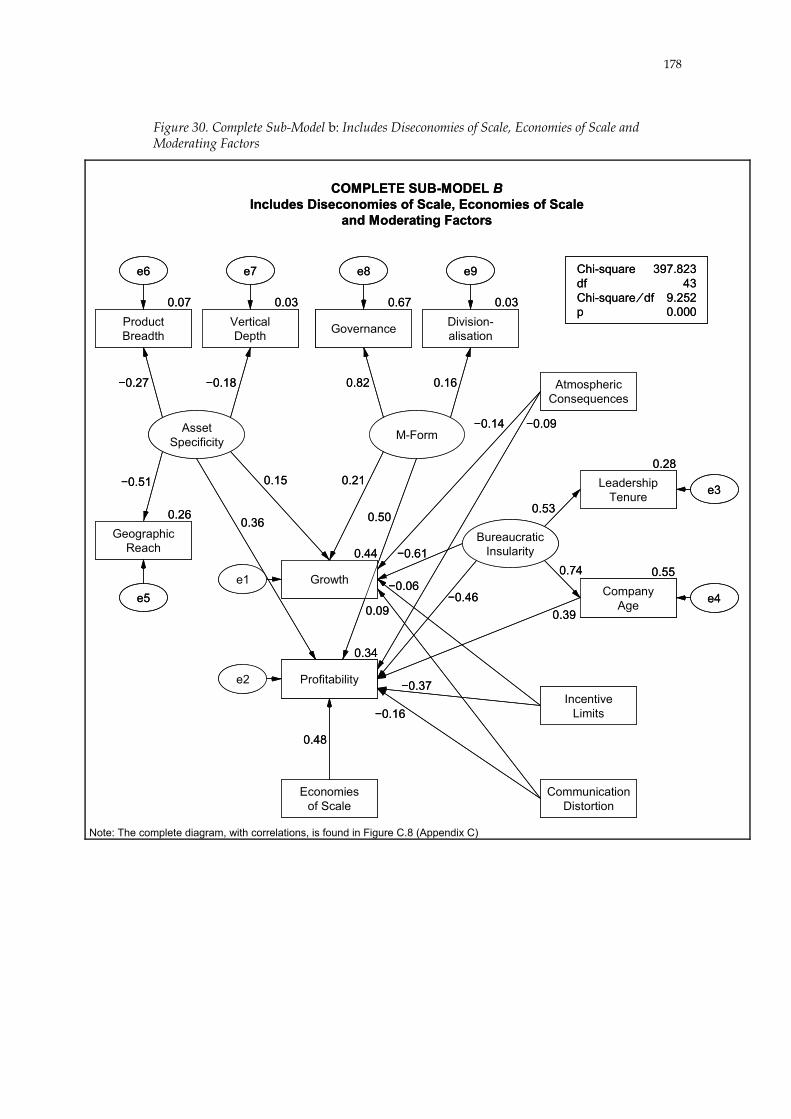
178
Figure 30. Complete Sub-Model b: Includes Diseconomies of Scale, Economies of Scale and Moderating Factors
COMPLETE SUB-MODEL BIncludes Diseconomies of Scale, Economies of Scale
and Moderating Factors
Profitability
Growth
e9
0.34
�0.37
0.55
0.28
�0.06�0.46
�0.09�0.14
0.67
Governance
0.03Division-alisation
0.82 0.16
0.09
�0.16
0.39
0.21
0.07ProductBreadth
0.03VerticalDepth
�0.27 �0.18
0.15
0.360.26
GeographicReach
e5
�0.51
0.50
0.48
�0.61
Chi-square 397.823df 43Chi-square � df 9.252p 0.000
e8e7e6
Governance
0.440.74
AssetSpecificity
AtmosphericConsequences
e1
e2
Economiesof Scale
CommunicationDistortion
M-Form
0.53
CompanyAge
LeadershipTenure e3
e4
BureaucraticInsularity
IncentiveLimits
Note: The complete diagram, with correlations, is found in Figure C.8 (Appendix C)

179
Figure 31. Matrix Representation of Complete Sub-Model b
MATRIX REPRESENTATION OF COMPLETE SUB-MODEL B
FormM�ySpecificitAsset�
ScaleofEconomies�DistortionionCommunicat�
LimitsIncentive�InsularityicBureaucrat�
esConsequenccAtmospheri�
7
6
5
4
3
2
1
−=======
divXgovernXvertXdrXforeignXfixhighXlevelsXrdXageXtenureXulabourX
B
A
9
8
7
6
5
4
3
2
1
===========
yofitabilitPr�Growth�
2
1==
evaYgrowthY
2
1==
��
���
�+�
�
���
�⋅+
���������
�
�
���������
�
�
��
���
�=�
�
���
�
2
1
2
1
7
6
5
4
3
2
1
27262524232221
171614131211
2
1
��
��
�������
�������������
��
0
����������������
�
�
����������������
�
�
+
���������
�
�
���������
�
�
����������������
�
�
����������������
�
�
=
����������������
�
�
����������������
�
�
B
A
9
8
7
3
2
7
6
5
4
3
2
1
XB7
XA7
X97
X96
X86
X76
X32
X22
B
A
9
8
7
6
5
4
3
2
1
�����
��
�������
11
1
1
XXXXXXXXXXX
��
���
�+�
�
���
���
���
�=�
�
���
�
2
1
2
1
2
1
��
11
YY
���������
�
�
���������
�
�
−−
−−
−−
−
=
7674
65
54535251
434241
3231
21
���
�������
���
�
��
���
�−
−=
21 � 0� =�
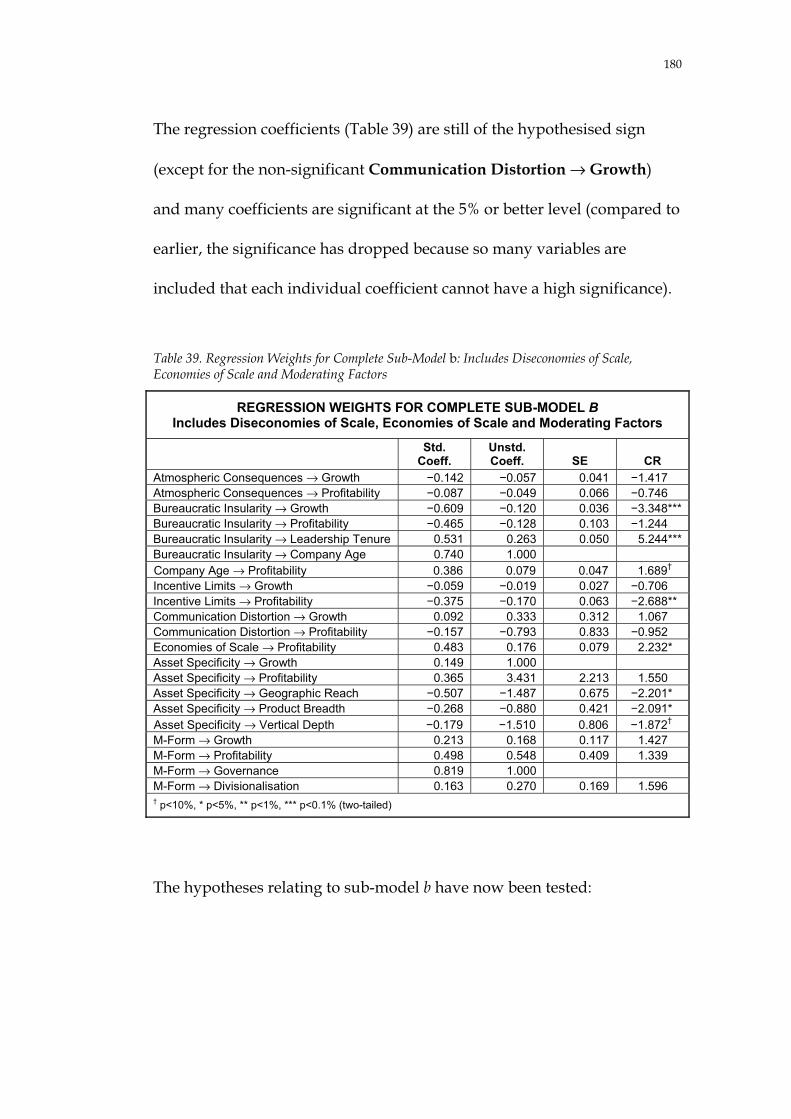
180
The regression coefficients (Table 39) are still of the hypothesised sign
(except for the non-significant Communication Distortion → Growth)
and many coefficients are significant at the 5% or better level (compared to
earlier, the significance has dropped because so many variables are
included that each individual coefficient cannot have a high significance).
Table 39. Regression Weights for Complete Sub-Model b: Includes Diseconomies of Scale, Economies of Scale and Moderating Factors
REGRESSION WEIGHTS FOR COMPLETE SUB-MODEL B Includes Diseconomies of Scale, Economies of Scale and Moderating Factors
Std. Coeff.
Unstd. Coeff. SE CR
Atmospheric Consequences → Growth �0.142 �0.057 0.041 �1.417***Atmospheric Consequences → Profitability �0.087 �0.049 0.066 �0.746***Bureaucratic Insularity → Growth �0.609 �0.120 0.036 �3.348***Bureaucratic Insularity → Profitability �0.465 �0.128 0.103 �1.244***Bureaucratic Insularity → Leadership Tenure 0.531 0.263 0.050 5.244***Bureaucratic Insularity → Company Age 0.740 1.000 Company Age → Profitability 0.386 0.079 0.047 1.689†** Incentive Limits → Growth �0.059 �0.019 0.027 �0.706***Incentive Limits → Profitability �0.375 �0.170 0.063 �2.688***Communication Distortion → Growth 0.092 0.333 0.312 1.067***Communication Distortion → Profitability �0.157 �0.793 0.833 �0.952***Economies of Scale → Profitability 0.483 0.176 0.079 2.232***Asset Specificity → Growth 0.149 1.000 Asset Specificity → Profitability 0.365 3.431 2.213 1.550***Asset Specificity → Geographic Reach �0.507 �1.487 0.675 �2.201***Asset Specificity → Product Breadth �0.268 �0.880 0.421 �2.091***Asset Specificity → Vertical Depth �0.179 �1.510 0.806 �1.872†** M-Form → Growth 0.213 0.168 0.117 1.427***M-Form → Profitability 0.498 0.548 0.409 1.339***M-Form → Governance 0.819 1.000 M-Form → Divisionalisation 0.163 0.270 0.169 1.596***† p<10%, * p<5%, ** p<1%, *** p<0.1% (two-tailed)
The hypotheses relating to sub-model b have now been tested:
181
H3a: Atmospheric consequences have a negative impact on the
performance of large firms.
Neither confirmed nor rejected. The regression coefficients have the
hypothesised sign (�11 = �0.14 and �21 = �0.09), but are not significant.
H3b: Bureaucratic insularity has a negative impact on the performance of
large firms
Confirmed. Bureaucratic insularity has a strong negative impact on
growth (�12 = �0.61) with a significance better than 0.1%. It also has a
strong negative impact on profitability (�22 = �0.46), but without meeting
threshold levels of significance.
H3c: Incentive limits have a negative impact on the performance of large
firms
Confirmed. Incentive limits have a strong negative impact on profitability
(�23 = �0.37) with better than 1% significance. The impact on growth is also
negative (�13 = �0.06), but the significance is low.
H3d: Communication distortion has a negative impact on the
performance of large firms

182
Neither confirmed nor rejected. Communication distortion has a non-
significant positive impact on growth (�14 = 0.09), contrary to the
hypothesis, and a non-significant negative impact on profitability
(�24 = �0.16), in line with the hypothesis. The inconclusive nature of the
finding may, however, agree with Mookherjee and Reichelstein (2001).
H4: Economies of scale increase the relative profitability of large firms
over smaller firms
Confirmed. The presence of economies of scale have a strong positive
influence on firm profitability (�25 = 0.48) at a significance better than the
5% level.
H5a: Large M-form firms perform better than large U-form firms
Possibly confirmed. M-form appears to lead to both higher growth
(�17 = 0.21) and higher profitability (�27 = 0.50). The significance is low in
both cases though, mainly because Divisionalisation reduces the
significance.
H5b: High internal asset specificity affects a firm’s performance
positively

183
Confirmed. Asset specificity has the predicted positive impact on both
growth (�16 = 0.15) and profitability (�26 = 0.36), but the significance is low.
The non-normal nature of the indicators probably leads to a large
underestimate of significance. Using the AS indicator, the significance is
better than the 1% level for growth and 10% level for profitability.
The practical significance is quite high at this point. The fit between the
theoretical framework and the statistical analysis for sub-model b is in
some ways surprisingly good, even though the test statistics vary in
strength.
6.2.4.2 Competing and Parsimonious Models
First, alternative models were tested to see if a competing model with
better fit could be constructed. Second, the chosen model was pruned for
parsimony so that only the important variables and relationships were
maintained. Hair et al. (1998, 614–616) and Bollen (1989, 289–305)
underpin the respecification approach used in the current research.
As the matrix representation in Figure 31 shows, the complete sub-model b
includes almost all possible causal relationships and correlations for
diseconomies of scale and economies of scale. The search for parsimony
therefore focused on testing changes in the relationships between the
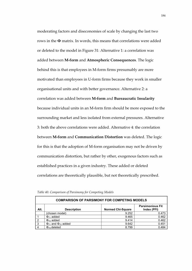
184
moderating factors and diseconomies of scale by changing the last two
rows in the � matrix. In words, this means that correlations were added
or deleted to the model in Figure 31: Alternative 1: a correlation was
added between M-form and Atmospheric Consequences. The logic
behind this is that employees in M-form firms presumably are more
motivated than employees in U-form firms because they work in smaller
organisational units and with better governance. Alternative 2: a
correlation was added between M-form and Bureaucratic Insularity
because individual units in an M-form firm should be more exposed to the
surrounding market and less isolated from external pressures. Alternative
3: both the above correlations were added. Alternative 4: the correlation
between M-form and Communication Distortion was deleted. The logic
for this is that the adoption of M-form organisation may not be driven by
communication distortion, but rather by other, exogenous factors such as
established practices in a given industry. These added or deleted
correlations are theoretically plausible, but not theoretically prescribed.
Table 40. Comparison of Parsimony for Competing Models
COMPARISON OF PARSIMONY FOR COMPETING MODELS
Alt. Description Normed Chi-Square Parsimonious Fit
Index (PFI) (chosen model) 9.252 0.4731 �71 added 9.465 0.4622 �72 added 9.414 0.4623 �71 and �72 added 9.642 0.4514 �74 deleted 8.799 0.484

185
Table 40 demonstrates that the alternative models are similar to the chosen
model. Alternative 4 is the only model with a better fit and parsimony, but
only marginally so. It was nevertheless rejected because the exclusion of
the correlation between M-Form and Communication Distortion does not
agree well with the theory.
The second step was to reduce the number of relationships in the model.
This builds on the assumption that while the theoretical predictions
captured in the hypotheses may be correct, they are not significant for
certain relationships and thus the theory should be modified. The pruned
model in Figure 32 uses the AS indicator defined in Section 6.2.3.2. The
pruned model also eliminates the non-significant regression coefficients
and correlations for the four diseconomies of scale factors. The squared
multiple correlation for Profitability improves dramatically from 0.34 to
0.64 (again because AS is more well-behaved than the three individual
measures (Product Depth, Geographic Reach and Vertical Depth) of
asset specificity), while it remains the same for Growth (0.44 versus 0.42).

186
Figure 32. Pruned Sub-Model b
PRUNED SUB-MODEL B
e9
0.64
�0.39
0.63
0.25
�0.70
�0.13
0.22
Governance
0.07Division-alisation
0.47 0.27
�0.18
0.59
0.360.32
0.52 0.79
0.46
�0.51
Chi-square 195.977df 28Chi-square � df 6.999p 0.000
e8
Governance
0.420.80
AtmosphericConsequences
e1
e2
Economiesof Scale
CommunicationDistortion
M-Form
0.50
AS
GrowthCompany
Age
LeadershipTenure e3
e4
BureaucraticInsularity
ProfitabilityIncentive
Limits
The normed chi-square improves from 9.252 to 6.999 and the normed fit
index is slightly higher at 0.980 versus 0.966. The parsimonious fit ratio is
0.424 compared to 0.473. The regression coefficients in Table 41 show that
Note: The complete diagram, with correlations, is found in Figure C.9 (Appendix C)

187
all coefficients have the hypothesised sign and all, except one, are
significant at better than the 10% level.
Table 41. Regression Weights for Pruned Sub-Model b
REGRESSION WEIGHTS FOR PRUNED SUB-MODEL B Std.
Coeff. Unstd. Coeff. SE CR
Atmospheric Consequences → Growth �0.131 �0.053 0.028 �1.926†** Bureaucratic Insularity → Growth �0.508 �0.092 0.013 �6.961***Bureaucratic Insularity → Profitability �0.695 �0.179 0.102 �1.754†** Bureaucratic Insularity → Leadership Tenure 0.500 0.231 0.045 5.107***Bureaucratic Insularity → Company Age 0.797 1.000 Company Age → Profitability 0.588 0.120 0.064 1.870†** Incentive Limits → Profitability �0.391 �0.178 0.047 �3.806***Communication Distortion → Profitability �0.182 �0.921 0.739 �1.247***Economies of Scale → Profitability 0.459 0.166 0.053 3.111***AS → Growth 0.318 0.386 0.120 3.231***AS → Profitability 0.525 0.902 0.433 2.081***M-Form → Growth 0.355 0.479 0.247 1.940†** M-Form → Profitability 0.786 1.499 0.859 1.746†** M-Form → Governance 0.474 1.000 M-Form → Divisionalisation 0.270 0.769 0.222 3.468***† p<10%, * p<5%, ** p<1%, *** p<0.1% (two-tailed)
The validity of the hypotheses has been strengthened. H3a is now
confirmed at the 10% level, H3b is (even more) strongly supported, H3c is
(more) strongly confirmed, H3d has increased its significance, but is still
not at the 10% level, H4 is strongly supported, H5a is supported at the 10%
level, while H5b is strongly supported.43
Finally, the 784 observations were randomly divided in two groups to test
whether similar results are achieved for different samples. The procedure
43 Full descriptions of the hypotheses are found on pages 119–120.

188
was repeated eight times and the critical ratios of the differences were
compiled for the main-effects model. Out of 104 possible differences, the
analysis indicated sixteen instances of differences significant at better than
the 10% level, of which ten where significant at better than the 5% level, of
which two were significant at better than the 1% level. This leads to the
conclusion that the results are homogenous across samples. Table 42
shows the results by regression coefficient for the main-effects model. No
single relationship appears to differ systematically between samples.

189
Table 42. Occurrence of Significant Critical Ratios of Differences during Random Sample Test
OCCURRENCE OF SIGNIFICANT CRITICAL RATIOS OF DIFFERENCES DURING RANDOM SAMPLE TEST
Regression Coefficient
Number of Observations No
Significant Difference
Better than 10% Sign.
Of Which Better than 5% Sign.
Of Which Better than 1% Sign. Total
Atmospheric Consequences → Growth 5 3 1 1 8Bureaucratic Insularity → Growth 7 1 1 0 8Bureaucratic Insularity → Profitability 8 0 0 0 8Bureaucratic Insularity → Tenure 5 3 3 0 8Company Age → Profitability 8 0 0 0 8Incentive Limits → Profitability 7 1 0 0 8Communication Distortion → Profitability 5 3 1 0 8Economies of Scale → Profitability 8 0 0 0 8AS → Growth 7 1 0 0 8AS → Profitability 7 1 1 0 8M-Form → Growth 6 2 2 1 8M-Form → Profitability 7 1 1 0 8M-Form → Divisionalisation 8 0 0 0 8Total 88 16 10 2 104 The next section summarises the findings from the statistical analyses of
the two sub-models and evaluates the five hypotheses.

190
6.3 SUMMARY OF FINDINGS FROM STRUCTURAL EQUATION MODELS
Table 43 shows the hypotheses and their associated findings. As was seen
throughout this chapter, most of the hypotheses were confirmed. The
findings seem to be robust for a number of reasons. The data were
screened and tested extensively (Chapter 5). They were found to be well-
behaved in most respects. The path diagrams confirm well with the
underlying theory. The indicators appear to reflect the unobserved
phenomena fairly well. Finally, the results were similar when random sub-
samples were used. It should be remembered though that the findings
apply only to one economic sector (manufacturing), in one country (the
United States), in one year (1998).

191
Table 43. Summary of Statistical Findings
SUMMARY OF STATISTICAL FINDINGSa
Hypothesis Test Result CR and Sign. Interpretation H1: Bureaucratic failure, in the form of atmospheric consequences, bureaucratic insularity, incentive limits and communication distortion, increases with firm size
�11(a) > 0 �11(a) = +0.92 +2.424 (p<1%) Confirmed
H2: Large firms exhibit economies of scale
�61(a) > 0 �61(a) = +0.60 +20.800 (p<0.1%) Confirmed
H3a: Atmospheric consequences have a negative impact on the performance of large firms
�11(b) < 0 �21(b) < 0
�11(b) = �0.13 –
�1.926 (p<10%) –
Confirmed
H3b: Bureaucratic insularity has a negative impact on the performance of large firms
�12(b) < 0 �22(b) < 0
�12(b) = �0.51 �22(b) = �0.70
�6.961 (p<0.1%) �1.754 (p<10%)
Confirmed
H3c: Incentive limits have a negative impact on the performance of large firms
�13(b) < 0 �23(b) < 0
– �23(b) = �0.39
– �3.806 (p<0.1%)
Confirmed
H3d: Communication distortion has a negative impact on the performance of large firms
�14(b) < 0 �24(b) < 0
– �24(b) = �0.18
– �1.247 (p=21.2%)
Inconclusive
H4: Economies of scale increase the relative profitability of large firms over smaller firms
�25(b) < 0 �25(b) = +0.46 +3.111 (p<1%) Confirmed
H5a: Large M-form firms perform better than large U-form firms
�17(b) > 0 �27(b) > 0
�17(b) = +0.36 �27(b) = +0.79
+1.940 (p<10%) +1.746 (p<10%)
Confirmed
H5b: High internal asset specificity affects a firm’s performance positively
�16(b) > 0 �26(b) > 0
�16(b) = +0.32 �26(b) = +0.52
+3.231 (p<1%) +2.081 (p<5%)
Confirmed
a For simplicity, the word ”confirmed” is used, although ”not rejected” is more accurate.
The practical significance of the statistical analyses is that both sub-model
a and sub-model b validate the theoretical framework. Both the main
analyses and the supporting analyses that tested particular aspects of the
theory (e.g., the separate analysis of the relationship between economies of
scale and growth in Section 6.2.2) are in line with the theoretical
predictions. It is not surprising that some of the relationships are weak
because executives have a tendency to exploit obvious opportunities for

192
improvement. Yet, most of the posited relationships in the theoretical
framework are non-trivial. Thus, the statistical analyses have delivered
practical insights.
Next, Chapter 7 explores the practical implications of the literature review
and the statistical analyses and ties the findings to the cost curves
discussed in Chapter 2. It also discusses the limitations of the research and
suggests avenues for further research.

193
7. INTERPRETATION AND DISCUSSION
Diseconomies of scale appear to be real. The literature overview discussed
the theoretical underpinnings of this thesis, indicating that a wide range of
theoretical development and empirical research, quantitative and
qualitative, supports pieces of the current theoretical predictions. The
statistical analysis section took a broader and more general approach to
testing the hypotheses, and nothing uncovered there disproved them. The
analyses also showed that diseconomies of scale vary in magnitude and
impact, and economies of scale and the moderating factors are important
when we try to understand the limits of the firm.
In the first section, the findings are summarised and interpreted by linking
them back to the cost curves discussed in Chapter 2 (pp. 14–17, above). By
doing this, the results from the somewhat unwieldy statistical analysis can
be presented in an effective shorthand. It is shown that the findings are
consistent with neoclassical theory and with transaction cost economics.
Building on this set of modified cost curves, further implications are
discussed, including the relative importance of the various factors that
affect a firm’s limits. The second section discusses the limitations of the
research, while the final section suggests paths for further research.

194
7.1 SUMMARY OF FINDINGS
The findings regarding the hypotheses are summarised in Table 44:
Table 44. Summary of Findings
SUMMARY OF FINDINGSa
Hypothesis Literature Finding Statistical Finding H1: Bureaucratic failure, in the form of atmospheric consequences, bureaucratic insularity, incentive limits and communication distortion, increases with firm size
Confirmed Confirmed
H2: Large firms exhibit economies of scale Confirmed Confirmed H3: Diseconomies of scale from bureaucratic failure have a negative impact on firm performance
Confirmed Confirmed
H3a: Atmospheric consequences have a negative impact on the performance of large firms
Confirmed Confirmed
H3b: Bureaucratic insularity has a negative impact on the performance of large firms
Confirmed Confirmed
H3c: Incentive limits have a negative impact on the performance of large firms
Confirmed Confirmed
H3d: Communication distortion has a negative impact on the performance of large firms
Confirmed Inconclusive
H4: Economies of scale increase the relative profitability of large firms over smaller firms
Inconclusive Confirmed
H5: Diseconomies of scale are moderated by two transaction cost-related factors: organisation form and asset specificity
Confirmed Confirmed
H5a: Large M-form firms perform better than large U-form firms
Confirmed Confirmed
H5b: High internal asset specificity affects a firm’s performance positively
Confirmed Confirmed
a For simplicity, the word ”confirmed” is used, although ”not rejected” is more accurate.
As is shown, the theoretical framework is supported by both the literature
and the statistical findings. It is now possible to interpret the findings by
returning to the neoclassical cost curves. First, the cost curve shown in
Figure 3 is modified to reflect the characteristics of diseconomies of scale,
economies of scale and the moderating factors. Second, a similar curve is

195
constructed for firm growth. Third, these two curves are combined to
show the overall impact of these two factors on firm performance.
Average cost. To begin with, the elongated U-shaped average total cost
curve44 used in neoclassical theory can be split into two parts: the average
production cost curve and the average transaction cost curve. Not much
evidence exists for what the relative magnitude of production and
transaction costs is. However, Wallis and North (1986) attempted to
quantify the relative contribution each type of cost makes to the overall
economy. They found that the transaction-cost part of the economy grew
from 25 per cent to 50 per cent of gross national product between 1890 and
1970 (p. 121). This suggests that an even split is a reasonable assumption.
The modified cost curves are depicted in a stylised fashion in Figure 33.
The top graph shows a curve for average production cost )( PAC consistent
with the findings in the current research. One characteristic of the curve is
important: the curve has a negative slope for all levels of firm output (Q).
This agrees with the view that economies of scale can be kept proprietary
to the firms that reap them. It also agrees with the statistical finding that
economies of scale are not exhausted at small firm sizes.
44 It would be more stringent to talk about ray average total costs because the firms analysed are
usually multi-product firms, but simplicity wins.

196
The middle graph in Figure 33 shows the average transaction cost curve
).( TAC The negative slope for smaller firms, indicating bureaucratic
economies of scale, is supported in the literature review (but was not
tested in the statistical analysis). The positive slope for larger firms,
indicating diseconomies of scale and bureaucratic failure, is supported by
both the literature and by the statistical analysis.
The middle graph also shows a shifted and slightly tilted average
transaction cost curve ).( TCA ′ The curve reflects the positive contribution
from the moderating factors. TCA ′ is supported by the literature and by
the statistical analysis. This analysis indicates that the shift can be quite
large.
Finally, the bottom graph in Figure 33 shows the average total cost curve
(AC), with a shifted curve CA ′ for the moderators (AC = PAC + TAC ;
CA ′ = PAC + TCA ′ ). The curve resembles the neoclassical curve in Figure
3. The question now is: where along this curve do firms operate? The
statistical analyses suggest that, on average, the largest firms in the sample
operate at outputs somewhere close to 2M′ in the upward-sloping region
of CA ′ . That is, they show some diseconomies of scale, but they also
benefit from economies of scale and they manage to take advantage of the
moderating factors.

197
Figure 33. Stylised Cost Curves
STYLISED COST CURVES
Output (Q)
Long-RunAverage
ProductionCost(ACP)
PAC
Output (Q)
Long-RunAverage
TransactionCost(ACT)
TAC
TCA ′
Output (Q)
Long-RunAverage
TotalCost(AC) AC
CA ′
1M 2M
2M ′
STYLISED COST CURVES
Output (Q)
Long-RunAverage
ProductionCost(ACP)
PAC
Output (Q)
Long-RunAverage
TransactionCost(ACT)
TAC
TCA ′
Output (Q)
Long-RunAverage
TotalCost(AC) AC
CA ′
1M 2M
2M ′
Output (Q)
Long-RunAverage
ProductionCost(ACP)
PAC
Output (Q)
Long-RunAverage
TransactionCost(ACT)
TAC
TCA ′
Output (Q)
Long-RunAverage
TotalCost(AC) AC
CA ′
1M 2M
2M ′
Growth. The underlying logic of the cost curves can also be applied to
firm growth. Figure 34 shows the same set of graphs as above for the

198
relationship between firm growth and output. The top graph illustrates
the relationship between growth and output, under the hypothetical
assumption that firms only have neoclassical production costs ).( PG
Neither the literature nor the statistical analysis indicated an influence (see
pp. 158–159, above) and thus the graph shows a constant relationship.
The middle graph in Figure 34 portrays the growth curve resulting from
bureaucratic, transaction cost-based, failure ).( TG The literature and the
statistical analysis make it fair to assume that TG should be monotonously
declining for increasing outputs. Again, the moderating influences can
shift the curve, which is illustrated by TG′ in the graph. The statistical
analysis indicates that the shift is smaller than in the case of average costs
).( CA ′
The bottom graph in Figure 34 convolutes the production- and
transaction-cost contributions to growth into overall growth (G). The
graph shows that the growth capacity of firms is steadily declining as a
function of output, but it can be moderated ).(G′ Interestingly, this
interpretation of the research contradicts Gibrat’s law of proportional
effects (1931, 74–81), which will be discussed later in this section.

199
Figure 34. Stylised Growth Curves
STYLISED GROWTH CURVES
Output (Q)
Long-RunGrowth
(Production)(GP)
PG
Output (Q)
Long-RunGrowth
(Transaction)(GT)
TG
TG′
Output (Q)
Long-RunGrowth
(G)
G
G′
STYLISED GROWTH CURVES
Output (Q)
Long-RunGrowth
(Production)(GP)
PG
Output (Q)
Long-RunGrowth
(Transaction)(GT)
TG
TG′
Output (Q)
Long-RunGrowth
(G)
G
G′
Output (Q)
Long-RunGrowth
(Production)(GP)
PG
Output (Q)
Long-RunGrowth
(Transaction)(GT)
TG
TG′
Output (Q)
Long-RunGrowth
(G)
G
G′
Performance. Finally, it is instructive to combine the cost and growth
curves to see how they jointly contribute to a firm’s performance (Figure
35). Other factors also contribute to firm performance and the graph shows

200
the partial contribution to performance.45 By convoluting the average total
cost (AC) and growth (G) curves, the partial performance curve � results.46
Several, perhaps speculative, interpretations can be derived from the
graph: (1) Firms operating at small outputs suffer from a lack of economies
of scale and this is most likely not compensated for by the higher relative
growth achievable by smaller firms. Thus, the slope 1k >0. (2) There is an
area where performance is fairly independent of firm size. On the one
hand, economies of scale should lead to steadily lower costs. On the other
hand, diminishing growth prospects reduce performance. On balance, the
analyses show that 2k <0, but only slightly so. (3) As diseconomies of scale
due to bureaucratic failure set in, the combined negative contribution of
increasing transaction costs and lower growth far outweigh economies of
scale. Thus, 3k <0. (4) The moderating factors shift the performance curve
outwards from � to � ′ and 3k < 3k′ <0, while 2M′ > 2M . That is, if firms
judiciously apply the moderating factors, then bureaucratic failure will set
in at a larger level of output and the impact from the failure will be less
severe.
45 Total performance (�TOT) is a function of, profitability(π), growth(G), risk(β) and other factors (ε):
�TOT = f(π, G, β, ε) = f(TR � TC, G, β, ε) = f(TR � AC · Q, G, β, ε). 46 The result from this convolution should not be taken for granted, but the statistical analysis
showed that AC and G are reasonably independent and that they should have similar weights.

201
The four interpretations above are supported by the literature review;
while the last three are supported by the statistical analysis (the statistical
analysis did not explore what happens at small firm sizes).
Figure 35. Stylised Partial Performance Curve
STYLISED PARTIAL PERFORMANCE CURVE
Output (Q)
Long-RunFactor
(AC and G)Contributions
to Performance
(�)
�
� ′1k
2k
3k 3k′
1M 2M
2M ′
STYLISED PARTIAL PERFORMANCE CURVE
Output (Q)
Long-RunFactor
(AC and G)Contributions
to Performance
(�)
�
� ′1k
2k
3k 3k′
1M 2M
2M ′
Output (Q)
Long-RunFactor
(AC and G)Contributions
to Performance
(�)
�
� ′1k
2k
3k 3k′
1M 2M
2M ′
The set of curves discussed above agree well with neoclassical theory (e.g.,
Panzar 1989) and transaction cost economics (e.g., Williamson 1975),
individually. The curves also agree with the joined perspectives on
production and transaction costs expressed by, for example, Riordan and
Williamson (1985) and Wallis and North (1986). What may make them
interesting is the unbundling of the production cost and transaction cost
contributions to firm performance, and the attempt to transform the
research findings into rough estimates of the shapes of the curves.

202
The conceptual curves depicted in Figures 33 to 35 can also be used to
show the shape of the data in the sample of 784 firms. This was done with
three analyses which replicated the cost (AC), growth (G) and partial
performance (� ) curves. Figures 36 to 38 show the resulting graphs, which
are surprisingly similar to the conceptual curves. It should be remembered
though, that the scatterplots presented are somewhat simplistic. They use
the sample data as is and no attempt was made to include control
variables or to make other corrections. The underlying assumptions and
SPSS scatterplots are found at http://canback.com/henley.htm in the file
Curves.spo.
First, Figure 36 reports the results for the cost curve (AC), which plots
average total cost (average factor costs, defined in Table 10, was used as
the proxy) against output (firm size was used as the proxy). A quadratic
regression line has been added to show the underlying trend in the data.
The data conform well to the conceptual AC curve in Figure 33.

203
Figure 36. Cost Curve for Current Sample
Output (Q)
Average Total Cost
(AC)
COST CURVE FOR CURRENT SAMPLE
Output (Q)
Average Total Cost
(AC)
COST CURVE FOR CURRENT SAMPLE
Second, growth data (5-year growth, defined in Table 9) were plotted
against output (Figure 37). Again, the curve has the predicted shape and
the quadratic regression line is similar to the conceptual G curve in Figure
34. The plot points are quite scattered though, and firms seem to have
considerable leeway to deviate from the growth rate prescribed by their
size.

204
Figure 37. Growth Curve for Current Sample
Output (Q)
5-Year Growth
(G)
GROWTH CURVE FOR CURRENT SAMPLE
Output (Q)
5-Year Growth
(G)
GROWTH CURVE FOR CURRENT SAMPLE
Third, the joint contribution to firm performance by the two factors is
shown in Figure 38. The average cost and growth data have been weighted
and added (� = �0.6AC + 0.4G, normalised). The weights for the current
sample came from an analysis of the relative contribution of AC and G to
Tobin’s Q, a commonly used composite measure of a firm’s performance
(e.g., Brainard and Tobin 1968; Lang and Stulz 1993).

205
The performance curve (� ) is not unlike the conceptual curve shown in
Figure 35. There is significant variation around the trend line, but overall
the data conform to the theoretical and empirical predictions.
Figure 38. Partial Performance Curve for Current Sample
Output (Q)
Factor(AC and G)
Contributions to
Performance (�)
PARTIAL PERFORMANCE CURVE FOR CURRENT SAMPLE
Output (Q)
Factor(AC and G)
Contributions to
Performance (�)
PARTIAL PERFORMANCE CURVE FOR CURRENT SAMPLE
These results now make it possible to prescribe certain remedies for
underperforming large firms, especially when poor performance stems
from low growth. Consider the impact of diseconomies of scale:
Bureaucratic insularity at both the institutional and individual levels
appears to be endemic in large firms, leading to low growth and low

206
profitability. Incentive limits negatively influence both growth and
profitability. Atmospheric consequences have a moderately negative
impact on growth, while communication distortion does not seem to be an
important source of diseconomies of scale.
Economies of scale can offset this to some extent; indeed, large firms tend
to exist in industries in which economies of scale are important. Moreover,
the negative effects of diseconomies of scale can be moderated by paying
attention to governance and organisational issues and by increasing asset
specificity. These factors more or less offset the diseconomies of scale for
large firms, resulting in a low overall correlation between performance
and size.
The diseconomies of scale exhibit a stronger negative influence on growth
than on profitability. This may indicate that Penrose’s suggestion that the
limits of a firm are related to dynamic factors rather than static factors is
correct (see p. 12, above). A large firm will find it relatively easy to
maximise profitability, but difficult to spur growth. An extension of this
argument is that Gibrat’s law of proportional effects (1931, 77) may not be
valid for growth and firm size, in line with corporate demography
research (Carroll and Hannan 2000, 315–319) and the findings of Sutton
(1997).

207
One way of expressing the impact of diseconomies of scale is to calculate
the market value of the largest firms if the diseconomies of scale did not
exist (and the economies of scale and moderating factors stayed the same).
The largest 100 firms in the sample had a combined market capitalisation
of 4.8 trillion dollars at the end of 1998, out of a total 6.7 trillion dollars for
the whole sample of 784 firms. If diseconomies of scale were reduced to
zero, then the expected growth of these firms would increase significantly
(around 4 percentage points) and the profitability would be somewhat
higher (around 0.5 percentage point). The combined effect (all other things
equal) might be an increase in market capitalisation from 4.8 trillion
dollars to 5.4 trillion dollars. It would also imply a higher growth in
productivity and a commensurate increase in the growth of GDP related to
the US manufacturing sector, up to 0.7 annual percentage points.47 This is
a crude estimate and it only serves to illustrate orders of magnitude.
47 This was calculated by taking the large companies’ contribution to the US GDP in 1998 (around
$650 billion; total GDP was $8,790 billion), and then increasing this number based on the increase in Tobin’s Q, estimated under the assumption of no diseconomies of scale. The estimate is a static assessment and the true impact is most likely lower.

208
7.2 LIMITATIONS OF THE RESEARCH
The current research is limited by a number of factors. Some of the
variables were not properly operationalised (for example vertical depth).
Other, more targeted, studies have used better definitions, but replicating
those definitions here would have expanded the work too much
(generalisability was prioritised over precision). As a result, simple, but
somewhat less reliable, definitions were used.
The selection of data also had a number of limitations. Potential industry
effects—while hypothesised to be small—were not incorporated. Data
were only collected for the manufacturing sector (strictly manufacturing,
construction, and mining). This sector represents only 22 per cent of the
US economy (26 per cent of the private sector) and includes less than half
of all large firms. In addition, international comparisons were not made
and longitudinal comparisons proved difficult to make.
Furthermore, no competing theories were introduced (see p. 11, above).
Although the transaction-cost-economics approach to studying
diseconomies of scale has yielded some insights, other theoretical
approaches may also contribute to the bureaucratic failure debate.
Finally, the statistical analyses consciously sacrificed precision at certain
points. For example, ordinal values were not analysed with polyserial and

209
polychoric correlations (see Section 5.1.2.3) and the influence of asset
specificity was not fully explored because these data were not normally
distributed. The model was therefore not optimised to extract the
maximum explanatory power.

210
7.3 FURTHER RESEARCH
Four avenues for further research may provide clarification and further
insights:
1. Proving the existence of diseconomies of scale by studying a more
narrowly defined problem such as focusing on an industry rather than
a whole economic sector. For example, earlier studies have explored
similar issues in the petrochemicals (Armour and Teece 1978), the
automotive (Masten, Meehan and Snyder 1989; Monteverde and Teece
1982) and the information technology industries (Rasmusen and
Zenger 1990; Zenger 1989, 1994). It may be worthwhile to build on this
body of knowledge and test particular aspects of the current work.
2. Expanding the analysis across geography and time. In particular, a
longitudinal study over a full business cycle would most likely lead to
more robust findings.
3. Finding better ways to operationalise unobserved diseconomies of
scale, perhaps by using panel data from primary research. Specifically,
communication distortion is often discussed qualitatively in the
literature, but the operationalisation of this concept remains elusive. In
this and other research efforts, the number of hierarchical levels in the
organisation was used as an indicator. It is not clear, however, why

211
information would be more distorted when it flows inside the firm,
than when it flows a similar distance in the market.
4. Replicating the current research with better statistical approaches and a
larger sample, with a particular eye towards industry effects. Industry
effects have proven difficult to quantify in general, but recent advances
in analytical techniques by, for example, McGahan and Porter (1997),
show that it may be possible to quantify these effects.
These suggestions are positivist and universal in nature. Clearly, other
approaches such as a phenomenological perspective can add insights into
the nature of diseconomies of scale.
The concluding chapter which now follows builds on the findings
discussed above and combines them with the researcher’s own experience
as a management consultant to large corporations.

212
8. CONCLUSION
Over the years, I have often been struck by how inefficient and
dysfunctional large corporations can be. Yet at the same time most of them
are immensely successful and deliver outstanding value to their
customers, while they perform well in the stock market. I base these
paradoxical comments on my interaction with large corporations, their
executives and employees during almost twenty years as a management
consultant at McKinsey & Company and Monitor Group. I struggled with
the paradox for many years and tried privately to reconcile the advantages
and disadvantages of large-scale organisation. In 1991, I happened to come
across Coase’s “The Nature of the Firm” (1937). After reading a twice-
faxed copy of the article on a (slow) bus between the terminal and an
airplane at Stuttgart airport, I became convinced that I could use
transaction cost economics to improve upon my advice to large
corporations, especially when working on strategic and organisational
development issues. This in turn led to the ambition to do formal research
on the limits of firm size. The research has confirmed many of my real-life
observations. Large corporations are inefficient in many ways, but for
good reasons. The benefits of large organisations are substantial, but there
are inescapable drawbacks as well.

213
The thesis demonstrates the need for research on limits of firm size, creates
a framework for thinking about the problem and indicates—based on the
literature survey and the statistical analysis—that there are real and
quantifiable diseconomies of size.
The heart of the research is a transaction cost economics-based framework
which combines four distinctive aspects of Williamson’s theory: (1) the
sources of firm-size limits: atmospheric consequences due to
specialisation, bureaucratic insularity, incentive limits of the employment
relation and communication distortion due to bounded rationality; (2) the
impact economies of scale have at the firm level; (3) the importance of
organisational form in reducing diseconomies; and (4) the positive
influence of high internal asset specificity on both transaction-cost and
production-cost diseconomies. The qualitative and quantitative analyses
conducted confirm the explanatory and predictive power of the theory. As
such, the research contributes to our understanding of the mechanisms
behind bureaucratic failure.
There are a number of real-life implications of the research. First, strategy
and structure appear to be intimately linked. Executives at large
corporations have to grapple with real trade-offs when they consider
expansion. Certain growth strategies are easier to execute than others, and
the choice of organisation has major implications for which strategies

214
make sense. Indeed, structure does not necessarily follow strategy;
strategy and structure inform each other continuously and forever.
Second, much of the rationale for mergers and acquisitions seems to be
weak, at best. Proponents of mergers typically argue that the resulting
larger entity after a merger will realise economies of scale, benefiting
customers and shareholders; in addition, they claim that growth will be
accelerated through the introduction of new products and services that
were previously too expensive to develop. But the analysis here shows
that although some economies of scale may be realised, they are likely to
be offset by diseconomies of scale. Furthermore, there is no evidence that
larger, merged entities innovate more and grow faster. Instead, the
opposite appears to be true: innovation and growth declines, on average.
This is particularly true in knowledge-intensive industries like
pharmaceuticals. To be sure, mergers and acquisitions often do make
sense. But executives need to think through how to minimise
diseconomies of scale, as well as to maximise moderating influences, when
post-merger integration is carried out.
Third, boards of directors may want to emphasise the importance of
executive renewal and the elimination of rigid processes to stimulate
growth. Old, large firms with entrenched management often find
themselves with a fundamental dilemma. There is no indication that they

215
can achieve above-average, profitable growth. They must choose either to
pay out excess cash flow to shareholders (as is often done) or to try to find
ways to break the firm’s bureaucratic insularity. Maximising the quality of
governance, which is part of the board’s fiduciary duties, appears to be an
important lever for maximising the value of large corporations.
Fourth, firms that strive for high internal asset specificity appear to be
better off than those that expand reach, breadth, or depth. This does not
imply that single-product or single-geography strategies are optimal
(because this reduces growth in the long run), but it does imply that any
expansion strategy should strive for high asset specificity and that some
firms are best off reducing their scope of activities. By and large, anecdotal
and empirical evidence suggests that this has happened over the last 20 to
30 years. “Focus on the core business” and “outsourcing” have been
hallmarks of restructuring programs for many years, and the current
research verifies that this is often a valid strategy.
Finally, in a world in which companies increasingly try to sell solutions
rather than basic products and services, incentive limits have become real
and problematic. In businesses that involve team selling or large product-
development efforts, attention should be paid to creating well-functioning
incentive schemes for employees. The superior productivity of research
and development in small firms, in which incentives are tailored to

216
individual performance, demonstrates why effective incentive schemes
matter.
It may be that the average large firm has neither a competitive advantage
nor a disadvantage when compared with small and mid-size firms.
However, the individual large firm will prosper or fade depending on
how well it manages diseconomies of scale.

217
APPENDIX A: LITERATURE REFERENCES PERTAINING TO DISECONOMIES OF SCALE
Adelman, M. A. 1978. Changes in Industrial Concentration. In Monopoly Power and Economic Performance, edited by Mansfield, E. New York: Norton.
Arrow, K. J. 1974. The Limits of Organization. New York: Norton.
———. 1983. Innovation in Large and Small Firms. In Entrepreneurship, edited by J. Ronen. Lexington, Mass.: Lexington Books.
Axtell, R. 1999. The Emergence of Firms in a Population of Agents: Local Increasing Returns, Unstable Nash Equilibria, and Power Law Size Distributions. Working paper, Washington: Center on Social and Economic Dynamics, Brookings Institution.
Bain, J. S. 1968. Industrial Organization. 2d ed. New York: Wiley.
Barnard, C. [1938] 1968. The Functions of the Executive. Reprint, with an introduction by K. R. Andrews. Cambridge: Harvard University Press. Original edition, Cambridge: Harvard University Press.
Blau, P. M. and M. W. Meyer. 1987. Bureaucracy in Modern Society. 3d ed. New York: McGraw-Hill.
Bock, B. 1978. New Numbers on Concentration: Fears and Facts. In Monopoly Power and Economic Performance, edited by E. Mansfield. New York: Norton.
Brock, J. W. 1987. Bigness Is the Problem, Not the Solution. Challenge 30 (July-August): 11–16.
Brown, C., J. Hamilton and J. Medoff. 1990. Employers Large and Small. Cambridge: Harvard University Press.
Carroll, G. R. and M. T. Hannan. 2000. The Demography of Corporations and Industries. Princeton: Princeton University Press.
Child, J. 1973. Predicting and Understanding Organization Structure. Administrative Science Quarterly 18 (2): 168–185.
Coase, R. H. 1937. The Nature of the Firm. Economica n.s., 4 (16): 386–405.
Cooper, A. C. 1964. R&D Is More Efficient in Small Companies. Harvard Business Review 42 (May-June): 75–83.
Crozier, M. 1964. The Bureaucratic Phenomenon. Chicago: University of Chicago Press.
Florence, P. S. 1933. The Logic of Industrial Organization. London: Kegan Paul.
Geanakoplos, J. and P. Milgrom. 1991. A Theory of Hierarchies Based on Limited Managerial Attention. Journal of the Japanese and International Economies 5 (3): 205–225.
Hannah, L. 1996. Marshall’s ‘Trees’ and the Global ‘Forest’: Were ‘Giant Redwoods’ Different? Paper read at NBER Conference, 19 October, at Cambridge, Mass.
Ibbotson Associates. 1999. Firm Size and Return. In Stocks, Bonds, Bills, and Inflation: 1999 Yearbook. Chicago: Ibbotson Associates.
Jensen, M. C. 1986. Agency Costs of Free Cash Flow, Corporate Finance, and Takeovers. American Economic Review 76 (2): 323–329.
———. 1989. Eclipse of the Public Corporation. Harvard Business Review 67 (September-October): 61–74.

218
Jensen, M. C. and W. H. Meckling. 1976. Theory of the Firm: Managerial Behavior, Agency Costs and Ownership Structure. Journal of Financial Economics 3 (4): 305–360.
Knight, F. H. [1921] 1964. Risk, Uncertainty and Profit. Reprint. New York: Augustus M. Kelley. Original edition, Boston: Houghton Mifflin.
Kwoka, J. E. 1980. Establishment Size, Wages, and Job Satisfaction: The Trade-Offs. In The Economics of Firm Size, Market Structure, and Social Performance, edited by J. J. Siegfried. Washington: Federal Trade Commission.
Lucas, R. E., Jr. 1978. On the Size Distribution of Business Firms. Bell Journal of Economics 9 (2): 508–523.
McAfee, R. P. and J. McMillan. 1995. Organizational Diseconomies of Scale. Journal of Economics and Management Strategy 4 (3): 399–426.
McConnell, J. L. 1945. Corporate Earnings by Size of Firm. Survey of Current Business 25 (May): 6–12.
Merton, R. K. 1957. Social Theory and Social Structure. Revised and enlarged ed. Glencoe, Ill.: Free Press.
Monsen, R. J. and A. Downs. 1965. A Theory of Large Managerial Firms. Journal of Political Economy 73 (3): 221–236.
Mookherjee, D. and S. Reichelstein. 2001. Incentives and Coordination in Hierarchies. Advances in Theoretical Economics 1 (1): Article 4. http://www.bepress.com/bejte/ advances/vol1/iss1/art4 (accessed 12 January 2002).
Mueller, W. F. and L. G. Hamm. 1974. Trends in Industrial Market Concentration, 1947 to 1970. Review of Economics and Statistics 56 (4): 511–520.
Nutter, G. W. 1951. The Extent of Enterprise Monopoly in the United States, 1899–1939. Chicago: University of Chicago Press.
Olson, M. 1982. The Rise and Decline of Nations: Economic Growth, Stagflation, and Social Rigidities. New Haven: Yale University Press.
Penrose, E. [1959] 1995. The Theory of the Growth of the Firm. 3d ed. New York: Oxford University Press. Original edition, New York: Wiley.
Peters, T. 1992. Rethinking Scale. California Management Review 35 (1): 7–29.
Pondy, L. R. 1969. Effects of Size, Complexity, and Ownership on Administrative Intensity. Administrative Science Quarterly 14 (1): 47–60.
Pugh, D. S., D. J. Hickson, C. R. Hinings and C. Turner. 1969. The Context of Organization Structures. Administrative Science Quarterly 14 (1): 91–114.
Qian, Y. 1994. Incentives and Loss of Control in an Optimal Hierarchy. Review of Economic Studies 61 (3): 527–544.
Rasmusen, E. and T. Zenger. 1990. Diseconomies of Scale in Employment Contracts. Journal of Law, Economics, and Organization 6 (1): 65–92.
Riordan, M. H. and O. E. Williamson. 1985. Asset Specificity and Economic Organization. International Journal of Industrial Organization 3 (4): 365–378.
Robertson, D. H. 1923. The Control of Industry. London: Nisbet.
Robinson, A. 1934. The Problem of Management and the Size of Firms. Economic Journal 44 (June): 242–257.

219
Scherer, F. M. 1976. Industrial Structure, Scale Economies, and Worker Alienation. In Essays on Industrial Organization in Honor of Joe S. Bain, edited by R. T. Masson and P. D. Qualls. Cambridge, Mass.: Ballinger.
Scherer, F. M. and D. Ross. 1990. Industrial Market Structure and Economic Performance. 3d ed. Boston: Houghton Mifflin.
Schmookler, J. 1972. The Size of Firm and the Growth of Knowledge. In Patents, Invention, and Economic Change, edited by Z. Griliches and L. Hurwicz. Cambridge: Harvard University Press.
Schumacher, E. F. 1989. Small Is Beautiful: Economics as if People Mattered. Perennial Library ed. New York: HarperCollins.
Silver, M. and R. Auster. 1969. Entrepreneurship, Profit, and Limits on Firm Size. Journal of Business 42 (April): 277–281.
Simon, H. A. [1947] 1976. Administrative Behavior. 3d ed. New York: Free Press. Original edition, New York: Macmillan.
Stigler, G. J. 1958. The Economies of Scale. Journal of Law and Economics 1 (October): 54–71.
———. 1974. The Case against Big Business. In Monopoly Power and Economic Performance, edited by Mansfield, E. New York: Norton.
Stinchcombe, A. L. 1965. Social Structure and Organizations. In Handbook of Organizations, edited by March, J. G. Chicago: Rand McNally.
Sutton, J. 1997. Gibrat’s Legacy. Journal of Economic Literature 35 (March): 40–59.
Williamson, O. E. 1967. Hierarchical Control and Optimum Firm Size. Journal of Political Economy 75 (2): 123–138.
———. 1975. Markets and Hierarchies: Analysis and Antitrust Implications. New York: Free Press.
———. 1984. The Incentive Limits of Firms: A Comparative Institutional Assessment of Bureaucracy. Weltwirtschaftliches Archiv 120 (4): 736–763.
———. 1985. The Economic Institutions of Capitalism. New York: Free Press.
———. 1996. The Mechanisms of Governance. New York: Oxford University Press.
Zenger, T. R. 1989. Organizational Diseconomies of Scale: Pooling vs. Separating Labor Contracts in Silicon Valley. PhD thesis, University of California, Los Angeles.
———. 1994. Explaining Organizational Diseconomies of Scale in R&D: Agency Problems and the Allocation of Engineering Talent, Ideas, and Effort by Firm Size. Management Science 40 (6): 708–729.

220
APPENDIX B: CORRELATION ANALYSES
Below follow two correlation analyses to support the structural equation
models. The purpose was to find whether the chosen definitions of size
and firm performance are meaningful from a statistical point-of-view. For
example, it could be that size measured as number of employees did not
correlate with other definitions such as revenue or assets. SPSS was used
for the correlation analyses. The appendix shows that robust and relevant
definitions can be construed for each variable.
DEFINITION OF SIZE
In line with the definitions of size in Section 2.2 (“Dimensions of Firm
Size”) number of employees (Employees), revenue (Sales), net assets (Net
Assets) and value added (Value Added), where correlated against each
other. These size-related variables are defined in Table B.1.

221
Table B.1. Size Variables
SIZE VARIABLES
Use Namea Labelb Type Description Metric Sources Size empl Employees Direct No. of employees ’000 Compustat Size sales Sales Direct Sales $M Compustat Size va Value Added Calculated Value added
defined as sales less cost of purchased goods and services � EBIT + labour cost + depreciation [va = ebit + labour + depr]
$M
Size na Net Assets Calculated Net assets defined as total assets less current assets plus current liabilities [na = ta � ca + cl]
$M
Size ebit EBIT Direct Earnings before interest and tax
$M Compustat
Size ta Total Assets Direct Total assets $M Compustat Size ca Current Assets Direct Current assets $M Compustat Size cl Current Liabilities Direct Current liabilities $M Compustat a The “Name” column shows the name given to the variable in SPSS and in Amos b The “Label” column shows the label given to the variable in SPSS and in Amos
Unsurprisingly, the four definitions are highly correlated (at better than
1% significance), as is seen in Table B.2.
Table B.2. Correlations between Various Definitions of Size
CORRELATIONS BETWEEN VARIOUS DEFINITIONS OF SIZE Employees Sales Value Added Net Assets
Employees Correlation 1** Sign. (2-tailed) N 784**
Sales Correlation 0.844** 1** Sign. (2-tailed) 0.000** N 784** 784**
Value Added
Correlation 0.923** 0.964** 1** Sign. (2-tailed) 0.000** 0.000** N 146** 146** 146**
Net Assets Correlation 0.724** 0.877** 0.925** 1**Sign. (2-tailed) 0.000** 0.000** 0.000** N 744** 744** 139** 744**
** Indicates correlations significant at the 1% level (2-tailed)

222
Based on the high correlations above, it was decided to perform the
structural equation analyses using one definition of size. The number of
employees was chosen to represent size because it is available for all firms
in the sample; it follows Child’s (1973) logic described in Section 2.2.2; it
has been used extensively in other studies of size-related issues (e.g., Hall
1986, 5–6; Kumar, Rajan and Zingales 1999, 12); and it is highly correlated
with the other variables. Section 2.2.2 also showed that sales is an
unsuitable measure and a separate analysis (not included in this thesis)
concluded that value added is too highly correlated with profitability to be
a good measure.
223
DEFINITION OF FIRM PERFORMANCE
Quantitative measures of firm performance include profitability measures
such as gross margin, net margin (i.e., return on sales), return on equity,
economic value added (i.e., return on equity less cost of equity), return on
capital employed; cash flow measures such as free cash flow over sales;
and growth measures such as 1-, 3-, 5- and 10-year historical revenue
growth.
Ideally, forward-looking measures such as expected profitability, cash
flow and growth should be used to measure a firm’s performance because
the current operating conditions (such as number of hierarchical levels or
organisation form) will influence future performance. However, the only
way to get such data without relying on analyst estimates is to perform the
analyses on a sample older than 5 years. This would significantly reduce
the number of variables in the model because most nonfinancial data are
not available five years back in time. Thus, the decision was made to use
current and historical data. The definitions are shown in Table B.3.

224
Table B.3. Performance Variables
PERFORMANCE VARIABLES
Use Namea Labelb Type Description Metric Sources Performance ros ROS Calculated Return on sales =
net income � sales % Compustat
Performance roe ROE Calculated Return on equity = net income � equity [roe = ni � equity]
%
Performance eva Profitability Calculated Economic value added defined as return on equity (ROE) less cost of equity (COE) [eva = roe � coe]
%
Performance fcf Free Cash Flow% Calculated Relative free cash flow defined as free cash flow � sales [fcf = fcftot � sales]
%
Performance growth3 Growth3 Direct 3-year compound annual sales growth
% Compustat
Performance growth Growth Direct 5-year compound annual sales growth
% Compustat
Performance growth10 Growth10 Direct 10-year compound annual sales growth
% Compustat
Performance fcftot Free Cash Flow Direct Free cash flow $M Compustat a The “Name” column shows the name given to the variable in SPSS and in Amos b The “Label” column shows the label given to the variable in SPSS and in Amos
Table B.4 shows the correlations between the seven alternative definitions
of firm performance. Return on sales (ROS), return on equity (ROE) and
economic value added (Profitability)48 are highly correlated (better than
1% significance). Economic value added was chosen as the
operationalisation of profitability because it most accurately measures
profitability and is available for all but two firms.
48 The variable could have been named EVA, but since this variable was chosen to represent
profitability in the statistical analyses, the generic variable name Profitability is used already here.

225
Growth measures show similarly high correlations. The best measure was
5-year growth (Growth)49 because it has higher correlation with 3- and 10-
year growth than they have with 5- and 10-, and 3- and 5-year growth,
respectively. It also has a large number of observations (756). Free cash
flow (FCF%) was not chosen as a measure of performance because it is too
prone to fluctuations between years. 50
Table B.4. Correlations between Various Definitions of Firm Performance
CORRELATIONS BETWEEN VARIOUS DEFINITIONS OF FIRM PERFORMANCE
ROS ROE
Profita-bility FCF% Growth3 Growth Growth10
ROS Correlation 1** Sign. (2-tailed) N 784**
ROE Correlation 0.683** 1** Sign. (2-tailed) 0.000** N 782** 782**
Profita-bility
Correlation 0.682** 0.993** 1** Sign. (2-tailed) 0.000** 0.000** N 781** 781** 781**
FCF% Correlation 0.370** 0.332** 0.331** 1** Sign. (2-tailed) 0.000** 0.000** 0.000** N 750** 750** 749** 750**
Growth3 Correlation 0.055** 0.020** 0.002** �0.017** 1** Sign. (2-tailed) 0.124** 0.570** 0.948** 0.635** N 777** 775** 774** 744** 777**
Growth Correlation 0.040** �0.007** �0.039** 0.012** 0.879** 1** Sign. (2-tailed) 0.272** 0.854** 0.280** 0.745** 0.000** N 756** 754** 753** 725** 756** 756**
Growth10 Correlation �0.020** �0.059** �0.098** 0.063** 0.719** 0.858** 1**Sign. (2-tailed) 0.605** 0.126** 0.011** 0.111** 0.000** 0.000** N 671** 669** 668** 643** 671** 668** 671**
* Indicates correlations significant at the 5% level (2-tailed) ** Indicates correlations significant at the 1% level (2-tailed)
49 Again, 5-year growth is labelled Growth, and not Growth5 since it was chosen as the indicator of
firm growth. 50 An additional benefit of using Profitability and Growth is that they correspond to Penrose’s
([1959] 1995) distinction between static economies (pp. 89–99) and diseconomies (pp. 12–13) of size (i.e., Profitability) and dynamic economies (pp. 99–101) and diseconomies (pp. 212–214) of growth (i.e., Growth).

226
It is worth noting (but is not surprising) that profitability and growth are
uncorrelated (�0.04), and that free cash flow is uncorrelated with growth
(0.01) and somewhat correlated with profitability (0.33).

227
APPENDIX C: COMPLETE PATH DIAGRAMS, INCLUDING CORRELATIONS
Figure C.1. Firm Performance versus Bureaucratic Insularity ................... 228 Figure C.2. Firm Performance versus Incentive Limits............................... 229 Figure C.3. Firm Performance versus Diseconomies of Scale:
Not Adjusted for Survivor Bias .......................................................... 230 Figure C.4. Firm Performance versus Diseconomies of Scale:
Adjusted for Survivor Bias .................................................................. 231 Figure C.5. Firm Performance versus Diseconomies of Scale and
Economies of Scale ............................................................................... 232 Figure C.6. Firm Performance versus Diseconomies of Scale,
Economies of Scale and M-Form Organisation ................................ 233 Figure C.7. Firm Performance versus Diseconomies of Scale,
Economies of Scale and Asset Specificity .......................................... 234 Figure C.8. Complete Sub-Model b ................................................................ 235 Figure C.9. Pruned Sub-Model b .................................................................... 236

228
Figure C.1. Firm Performance versus Bureaucratic Insularity
FIRM PERFORMANCE VERSUS BUREAUCRATIC INSULARITY
0.23
Growth
�0.39
e1
0.03
Profitability0.19
e2
0.38
�0.18
�0.11
CompanyAge
LeadershipTenure
FIRM PERFORMANCE VERSUS BUREAUCRATIC INSULARITY
0.23
Growth
�0.39
e1
0.03
Profitability0.19
e2
0.38
�0.18
�0.11
CompanyAge
LeadershipTenure

229
Figure C.2. Firm Performance versus Incentive Limits
FIRM PERFORMANCE VERSUS INCENTIVE LIMITS
0.20
Growthe1
0.03
Profitabilitye2
�0.01
�0.10
�0.29�0.46
0.12
IncentiveLimits
CompanyAge
FIRM PERFORMANCE VERSUS INCENTIVE LIMITS
0.20
Growthe1
0.03
Profitabilitye2
�0.01
�0.10
�0.29�0.46
0.12
IncentiveLimits
CompanyAge

230
Figure C.3. Firm Performance versus Diseconomies of Scale: Not Adjusted for Survivor Bias
FIRM PERFORMANCE VERSUS DISECONOMIES OF SCALENot adjusted for Survivor Bias
Chi-square 16.490df 4Chi-square � df 4.123p 0.002
Growth
Profitability
0.08
�0.01
0.54
0.25
�0.090.26
�0.21�0.18
0.11
0.01
�0.630.43
�0.37
0.38
0.16
0.13
0.12
0.05
0.36
0.74
IncentiveLimits
AtmosphericConsequences
e1
e2
BureaucraticInsularity
CommunicationDistortion
0.50
LeadershipTenure
e4CompanyAge
e3

231
Figure C.4. Firm Performance versus Diseconomies of Scale: Adjusted for Survivor Bias
FIRM PERFORMANCE VERSUS DISECONOMIES OF SCALEAdjusted for Survivor Bias
Chi-square 14.011df 3Chi-square � df 4.670p 0.003
Growth
Profitability
0.09
�0.17
0.51
0.28
�0.12�0.33
�0.06�0.15
0.14
0.14
0.32
�0.670.45
�0.38
0.40
0.16
0.12
�0.05
0.05
0.39
0.71
IncentiveLimits
AtmosphericConsequences
e1
e2
BureaucraticInsularity
CommunicationDistortion
0.53
CompanyAge e4
LeadershipTenure e3

232
Figure C.5. Firm Performance versus Diseconomies of Scale and Economies of Scale
Growth
FIRM PERFORMANCE VERSUS DISECONOMIES OF SCALEAND ECONOMIES OF SCALE
Chi-square 8.995df 5Chi-square � df 1.799p 0.109
0.12
�0.25
0.49
0.28
�0.12�0.32
�0.14�0.08
0.15
�0.01
0.30
0.27
�0.720.44
�0.34
0.44
0.40
0.56
0.10
0.22
�0.04
0.00
0.34
0.28
0.34
0.70
AtmosphericConsequences
e1
e2
BureaucraticInsularity
Economiesof Scale
CommunicationDistortion
0.53
IncentiveLimits
CompanyAge e4
LeadershipTenure e3
Profitability

233
Figure C.6. Firm Performance versus Diseconomies of Scale, Economies of Scale and M-Form Organisation
FIRM PERFORMANCE VERSUS DISECONOMIES OF SCALE,ECONOMIES OF SCALE AND M-FORM ORGANISATION
e9
0.29
�0.31
0.48
0.29
�0.12�0.43
�0.09�0.08
0.63
Governance
0.01Division-alisation
0.79 0.09
�0.06
0.36
0.21
0.38
0.28
�0.71
Chi-square 75.618df 17Chi-square � df 4.448p 0.000
e8
Governance
0.50
�0.34
0.43
0.40
0.55
0.10
0.21
�0.22
�0.02
0.33
0.28
0.33
0.70
AtmosphericConsequences
e1
e2
Economiesof Scale
M-Form
0.53
0.12Leadership
Tenure e3
e4
BureaucraticInsularity
Growth
IncentiveLimits
CommunicationDistortion
CompanyAge
Profitability
0.11
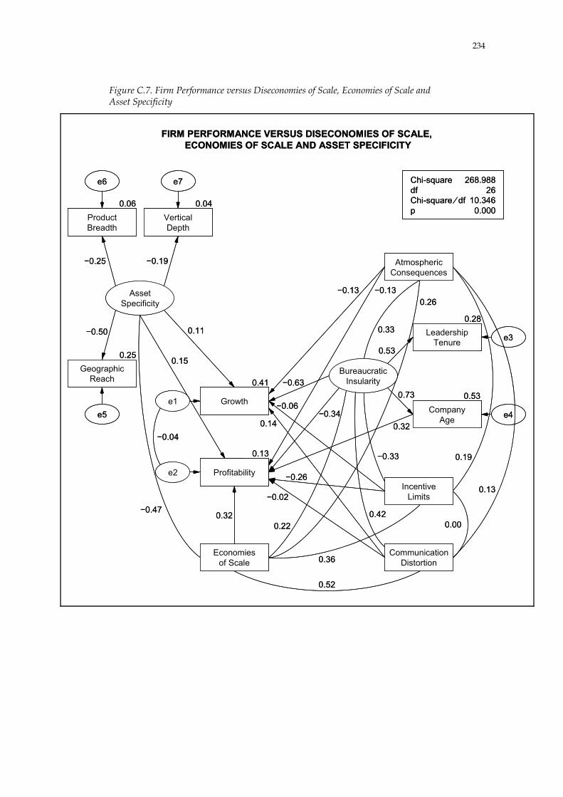
234
Figure C.7. Firm Performance versus Diseconomies of Scale, Economies of Scale and Asset Specificity
Profitability
FIRM PERFORMANCE VERSUS DISECONOMIES OF SCALE,ECONOMIES OF SCALE AND ASSET SPECIFICITY
�0.26
0.53
0.28
�0.06�0.34
�0.13�0.13
0.14
�0.02
0.32
0.06ProductBreadth
0.04VerticalDepth
�0.25 �0.19
0.11
0.150.25
GeographicReach
e5
�0.50
0.32
�0.63
Chi-square 268.988df 26Chi-square � df 10.346p 0.000
e7e6
0.41
�0.33
0.42
0.36
0.52
0.13
0.19
�0.04
0.00
�0.47
0.26
0.22
0.33
0.73
AssetSpecificity
AtmosphericConsequences
e1
e2
BureaucraticInsularity
Economiesof Scale
CommunicationDistortion
0.53e3Leadership
Tenure
e4Growth
IncentiveLimits
CompanyAge
0.13

235
Figure C.8. Complete Sub-Model b: Includes Diseconomies of Scale, Economies of Scale and Moderating Factors
Profitability
Growth
COMPLETE SUB-MODEL BIncludes Diseconomies of Scale, Economies of Scale
and Moderating Factors
e9
0.34
�0.37
0.55
0.28
�0.06�0.46
�0.09�0.14
0.67
Governance
0.03Division-alisation
0.82 0.16
0.09
�0.16
0.39
0.21
0.07ProductBreadth
0.03VerticalDepth
�0.27 �0.18
0.15
0.360.26
GeographicReach
e5
�0.51
0.50
0.48
�0.61
Chi-square 397.823df 43Chi-square � df 9.252p 0.000
e8e7e6
Governance
0.44
�0.33
0.41
0.37
0.51
0.13
0.17
�0.21
�0.02
�0.43
�0.30
0.24
0.22
0.31
0.74
AssetSpecificity
AtmosphericConsequences
e1
e2
Economiesof Scale
CommunicationDistortion
M-Form
0.53
0.11
CompanyAge
LeadershipTenure e3
e4
BureaucraticInsularity
IncentiveLimits

236
Figure C.9. Pruned Sub-Model b
PRUNED SUB-MODEL B
e9
0.64
�0.39
0.63
0.25
�0.70
�0.13
0.22
Governance
0.07Division-alisation
0.47 0.27
�0.18
0.59
0.360.32
0.52 0.79
0.46
�0.51
Chi-square 195.977df 28Chi-square � df 6.999p 0.000
e8
Governance
0.42
�0.31
0.35
0.40
0.52
0.21
�0.52
�0.20
�0.49
0.18
0.20
0.19
0.80
AtmosphericConsequences
e1
e2
Economiesof Scale
CommunicationDistortion
M-Form
0.50
0.13
AS
GrowthCompany
Age
LeadershipTenure e3
e4
BureaucraticInsularity
ProfitabilityIncentive
Limits

237
REFERENCES
Adams, W. and J. W. Brock. 1986. The Bigness Complex: Industry, Labor, and Government in the American Economy. New York: Pantheon.
Adelman, M. A. 1978. Changes in Industrial Concentration. In Monopoly Power and Economic Performance, edited by E. Mansfield. New York: Norton.
Allen, B. T. 1976. Average Concentration in Manufacturing, 1947–1972. Journal of Economic Issues 10 (September): 664–673.
Arbuckle, J. L. 1996. Full Information Estimation in the Presence of Incomplete Data. In Advanced Structural Equation Modeling: Issues and Techniques, edited by G. A. Marcoulides and R. E. Schumacker. Mahwah, N.J.: Lawrence Erlbaum Associates.
Arbuckle, J. L. and W. Wothke. 1999. Amos 4.0 User’s Guide. Chicago: SPSS, Inc.
Armour, H. O. and D. J. Teece. 1978. Organizational Structure and Economic Performance: A Test of the Multidivisional Hypothesis. Bell Journal of Economics 9 (1): 106–122.
———. 1980. Vertical Integration and Technological Innovation. Review of Economics and Statistics 62 (August): 470–474.
Arrow, K. J. 1964. Control in Large Organizations. Management Science 10 (3): 397–408.
———. 1974. The Limits of Organization. New York: Norton.
———. 1983. Innovation in Large and Small Firms. In Entrepreneurship, edited by J. Ronen. Lexington, Mass.: Lexington Books.
Aw, B. and G. Batra. 1998. Firm Size and the Pattern of Diversification. International Journal of Industrial Organization 16 (3): 313–331.
Axtell, R. 1999. The Emergence of Firms in a Population of Agents: Local Increasing Returns, Unstable Nash Equilibria, and Power Law Size Distributions. Working paper, Washington: Center on Social and Economic Dynamics, Brookings Institution.
Bain, J. S. 1968. Industrial Organization. 2d ed. New York: Wiley.

238
———. 1978. The General Explanation of the Development of Concentration. In Monopoly Power and Economic Performance, edited by E. Mansfield. New York: Norton.
Bane, W. T. and F. Neubauer. 1981. Diversification and the Failure of New Foreign Activities. Strategic Management Journal 2 (3): 219–233.
Barnard, C. [1938] 1968. The Functions of the Executive. Revised ed. Reprint, with an introduction by K. R. Andrews. Cambridge: Harvard University Press. Original edition, Cambridge: Harvard University Press.
Berle, A. A. and G. C. Means. [1932] 1991. The Modern Corporation and Private Property. Revised ed. Reprint, with a new introduction by M. L. Weidenbaum and M. Jensen. New Brunswick, N.J.: Transaction Publishers. Original edition, New York: Commerce Clearing House.
Bhidé, A. 1990. Reversing Corporate Diversification. Journal of Applied Corporate Finance 3 (2): 70–81.
Blau, P. M. and M. W. Meyer. 1987. Bureaucracy in Modern Society. 3d ed. New York: McGraw-Hill.
Bock, B. 1978. New Numbers on Concentration: Fears and Facts. In Monopoly Power and Economic Performance, edited by E. Mansfield. New York: Norton.
Bollen, K. A. 1989. Structural Equations with Latent Variables. New York: Wiley.
Bolton, P. and D. S. Scharfstein. 1998. Corporate Finance, the Theory of the Firm, and Organizations. Journal of Economic Perspectives 12 (4): 95–114.
Brainard, W. C. and J. Tobin. 1968. Pitfalls in Financial Model Building. American Economic Review 58 (May): 99–122.
Brock, J. W. 1987. Bigness Is the Problem, Not the Solution. Challenge 30 (July-August): 11–16.
Brown, C., J. Hamilton and J. Medoff. 1990. Employers Large and Small. Cambridge: Harvard University Press.
Byrne, J. A. 2000. Special Report: Corporate Governance. Business Week, 24 January, 142–152.

239
CalPERS. 1999. Corporate Governance Screen. http:// www.calpers-governance.org/alert/focus/1999/screen.asp (accessed 12 September 2000).
Canbäck, S. 2002. Supporting Thesis Materials. http://canback.com/ henley.htm (accessed 17 January 2002).
Carroll, G. R. and M. T. Hannan. 2000. The Demography of Corporations and Industries. Princeton: Princeton University Press.
Chandler, A. D., Jr. 1962. Strategy and Structure: Chapters in the History of the American Industrial Enterprise. Cambridge: MIT Press.
———. 1977. The Visible Hand. Cambridge, Mass.: Belknap.
———. 1982. Evolution of the Large Industrial Corporation: An Evolution of the Transaction-Cost Approach. Business and Economic History 2d series, 11: 116–134.
———. 1990. Scale and Scope: The Dynamics of Industrial Capitalism. Cambridge, Mass.: Belknap.
———. 1992. The Emergence of Managerial Capitalism. In The Sociology of Economic Life, edited by M. Granovetter and R. Swedberg. Boulder, Colo.: Westview Press.
Chandler, A. D., Jr. and H. Daems, eds. 1980. Managerial Hierarchies: Comparative Perspectives on the Rise of the Modern Industrial Enterprise. Cambridge: Harvard University Press.
Child, J. 1973. Predicting and Understanding Organization Structure. Administrative Science Quarterly 18 (2): 168–185.
Coase, R. H. 1937. The Nature of the Firm. Economica n.s., 4 (16): 386–405.
———. 1993a. 1991 Nobel Lecture: The Institutional Structure of Production. In The Nature of the Firm: Origins, Evolution, and Development, edited by O. E. Williamson and S. G. Winter. New York: Oxford University Press.
———. 1993b. The Nature of the Firm: Meaning. In The Nature of the Firm: Origins, Evolution, and Development, edited by O. E. Williamson and S. G. Winter. New York: Oxford University Press.
240
———. 1993c. The Nature of the Firm: Origin. In The Nature of the Firm: Origins, Evolution, and Development, edited by O. E. Williamson and S. G. Winter. New York: Oxford University Press.
Colvin, G. 2000. America’s Most Admired Companies. Fortune, 21 February, 108–117, F1–F7.
Comment, R. and G. A. Jarrell. 1995. Corporate Focus and Stock Returns. Journal of Financial Economics 37 (1): 67–87.
Cooper, A. C. 1964. R&D Is More Efficient in Small Companies. Harvard Business Review 42 (May-June): 75–83.
Council of Economic Advisers. 1998. Economic Report of the President. Washington: U.S. Government Printing Office.
———. 2002. Economic Report of the President. Washington: U.S. Government Printing Office.
Crozier, M. 1964. The Bureaucratic Phenomenon. Chicago: University of Chicago Press.
D’Aveni, R. A. and D. J. Ravenscraft. 1994. Economies of Integration versus Bureaucracy Costs: Does Vertical Integration Improve Performance? Academy of Management Journal 37 (5): 1167–1206.
DeCarlo, L. T. 1997. normtest.sps [SPSS macro], November. http:// www.columbia.edu/~ld208/ (accessed 20 February 2001).
Easterby-Smith, M., R. Thorpe and A. Lowe. 1991. Management Research: An Introduction. London: Sage.
Eatwell, J., M. Milgate and P. Newman, eds. 1987. The New Palgrave: A Dictionary of Economics. 3 vols. New York: Stockton Press.
Farrell, C. 1998. Does Wharton’s Jeremy Siegel Have Alan Greenspan’s Ear? Business Week, 13 July.
Fligstein, N. 1985. The Spread of the Multidivision Form among Large Firms, 1919–1979. American Sociological Review 50 (June): 377–391.
Florence, P. S. 1933. The Logic of Industrial Organization. London: Kegan Paul.
Fortune. 1995a. The Fortune 500, 1994. Fortune, 15 May, 165–227, F1–F64.

241
———. 1995b. The Fortune Global 500, 1994. Fortune, 7 August, 123–136, F1–F42.
Gatty, R. 1966. Multivariate Analysis for Marketing Research: An Evaluation. Applied Statistics 15 (November): 157–172.
Geanakoplos, J. and P. Milgrom. 1991. A Theory of Hierarchies Based on Limited Managerial Attention. Journal of the Japanese and International Economies 5 (3): 205–225.
Gibrat, R. 1931. Les inégalités économiques. Paris: Librairie du Recueil Sirey.
Grossman, S. J. and O. D. Hart. 1986. The Costs and Benefits of Ownership: A Theory of Vertical and Lateral Integration. Journal of Political Economy 94 (4): 691–719.
Hair, J. F., Jr., R. E. Anderson, R. L. Tatham and W. C. Black. 1998. Multivariate Data Analysis. 5th ed. Upper Saddle River, N.J.: Prentice Hall.
Hall, B. H. 1986. The Relationship between Firm Size and Firm Growth in the U.S. Manufacturing Sector. Working paper, Cambridge, Mass.: NBER.
Hannah, L. 1996. Marshall’s ‘Trees’ and the Global ‘Forest’: Were ‘Giant Redwoods’ Different? Paper read at NBER Conference, 19 October, at Cambridge, Mass.
Hardyck, C. D. and L. F. Petrinovich. 1976. Introduction to Statistics for the Behavioral Sciences. 2d ed. Philadelphia: Saunders.
Harrigan, K. R. 1986. Matching Vertical Integration Strategies to Competitive Conditions. Strategic Management Journal 7 (6): 535–555.
Hart, O. 1995. Firms, Contracts, and Financial Structure. Oxford: Clarendon Press.
Hayduk, L. A. 1996. LISREL Issues, Debates, and Strategies. Baltimore: Johns Hopkins University Press.
Holmström, B. and J. Roberts. 1998. The Boundaries of the Firm Revisited. Journal of Economic Perspectives 12 (4): 73–94.
Holmström, B. R. and J. Tirole. 1989. The Theory of the Firm. In Handbook of Industrial Organization, Vol. 1, edited by R. Schmalensee and R. Willig. New York: North-Holland.

242
Ibbotson Associates. 1999. Firm Size and Return. In Stocks, Bonds, Bills, and Inflation: 1999 Yearbook. Chicago: Ibbotson Associates.
Ijiri, Y. and H. A. Simon. 1964. Business Firm Growth and Size. American Economic Review 54 (2): 77–89.
Investor Responsibility Research Center (IRRC). 1999. Board Practices 1999: The Structure and Compensation of Board of Directors at S&P Super 1,500 Companies. Washington: Investor Responsibility Research Center.
Jensen, M. C. 1986. Agency Costs of Free Cash Flow, Corporate Finance, and Takeovers. American Economic Review 76 (2): 323–329.
———. 1988. Takeovers: Their Causes and Consequences. Journal of Economic Perspectives 2 (1): 21–48.
———. 1989. Eclipse of the Public Corporation. Harvard Business Review 67 (September-October): 61–74.
———. 2000. A Theory of the Firm: Governance, Residual Claims, and Organizational Forms. Cambridge: Harvard University Press.
Jensen, M. C. and W. H. Meckling. 1976. Theory of the Firm: Managerial Behavior, Agency Costs and Ownership Structure. Journal of Financial Economics 3 (4): 305–360.
Jöreskog, K. and D. Sörbom. 1996. LISREL 8: User’s Reference Guide. Chicago: Scientific Software International.
Joskow, P. L. 1993. Asset Specificity and the Structure of Vertical Relationships: Empirical Evidence. In The Nature of the Firm: Origins, Evolution, and Development, edited by O. E. Williamson and S. G. Winter. New York: Oxford University Press.
Kelloway, E. K. 1998. Using LISREL for Structural Equation Modeling. Thousand Oaks, Calif.: Sage.
Kimberly, J. R. 1976. Organizational Size and the Structuralist Perspective: A Review, Critique and Proposal. Administrative Science Quarterly 21 (4): 571–597.
Klier, T. H. 1993. Transaction Cost Theory and Just-in-Time Manufacturing: A New Look at Vertical Integration in the United States Automobile Market. PhD thesis, Department of Economics, Michigan State University.

243
Knight, F. H. [1921] 1964. Risk, Uncertainty and Profit. Reprint, New York: Augustus M. Kelley. Original edition, Boston: Houghton Mifflin.
Krickx, G. A. M. 1988. Historical Evidence on the Evolution of Vertical Exchange Mechanisms: Examples from the Computer Systems Industry. PhD thesis, University of California, Los Angeles.
Kumar, K. B., R. G. Rajan and L. Zingales. 1999. What Determines Firm Size? Working paper, Cambridge, Mass.: NBER.
Kwoka, J. E. 1980. Establishment Size, Wages, and Job Satisfaction: The Trade-Offs. In The Economics of Firm Size, Market Structure, and Social Performance, edited by J. J. Siegfried. Washington: Federal Trade Commission.
Lang, L. H. P. and R. M. Stulz. 1993. Tobin’s Q, Corporate Diversification and Firm Performance. Working paper, Cambridge, Mass.: NBER.
Levy, D. T. 1981. The Transactions Cost Approach to Vertical Integration: An Empirical Examination. PhD thesis, University of California, Los Angeles.
Lucas, R. E., Jr. 1978. On the Size Distribution of Business Firms. Bell Journal of Economics 9 (2): 508–523.
Mahoney, J. T. 1989. Organizational Rationalization and Innovation: Vertical Integration and Multidivisional Organization. PhD thesis, University of Pennsylvania.
———. 1992. The Choice of Organizational Form: Vertical Financial Ownership versus Other Methods of Vertical Integration. Strategic Management Journal 13 (8): 559–584.
Mankiw, N. G. 1998. Principles of Economics. Fort Worth, Tex.: Dryden.
Marglin, S. A. 1974. What Do Bosses Do? The Origins of Hierarchy in Capitalist Production. Review of Radical Political Economics 6 (2): 60-112.
Marshall, A. [1920] 1982. Principles of Economics: An Introductory Volume. 8th ed. Philadelphia: Porcupine Press. Original edition, London: Macmillan.
Maruyama, G. M. 1998. Basics of Structural Equation Modeling. Thousand Oaks, Calif.: Sage.

244
Mas-Colell, A., M. D. Whinston and J. R. Green. 1995. Microeconomic Theory. New York: Oxford University Press.
Masten, S. E. 1982. Transaction Costs, Institutional Choice and the Organization of Production. PhD thesis, University of Pennsylvania.
———. 1984. The Organization of Production: Evidence from the Aerospace Industry. Journal of Law and Economics 27 (October): 403–417.
Masten, S. E., J. W. Meehan, Jr. and E. A. Snyder. 1989. Vertical Integration in the US Auto Industry: A Note on the Influence of Transaction Specific Assets. Journal of Economic Behavior and Organization 12 (2): 265–273.
———. 1991. The Costs of Organization. Journal of Law, Economics and Organization 7 (1): 1–25.
McAfee, R. P. and J. McMillan. 1995. Organizational Diseconomies of Scale. Journal of Economics and Management Strategy 4 (3): 399–426.
McConnell, J. L. 1945. Corporate Earnings by Size of Firm. Survey of Current Business 25 (May): 6–12.
McGahan, A. M. and M. E. Porter. 1997. How Much Does Industry Matter, Really? Strategic Management Journal 18 (Summer): 15–30.
Merton, R. K. 1957. Social Theory and Social Structure. Revised and enlarged ed. Glencoe, Ill.: Free Press.
Monsen, R. J. and A. Downs. 1965. A Theory of Large Managerial Firms. Journal of Political Economy 73 (3): 221–236.
Monteverde, K. and D. J. Teece. 1982. Supplier Switching Costs and Vertical Integration in the Automobile Industry. Bell Journal of Economics 13 (1): 206–213.
Mookherjee, D. and S. Reichelstein. 2001. Incentives and Coordination in Hierarchies. Advances in Theoretical Economics 1 (1): Article 4. http://www.bepress.com/bejte/advances/vol1/iss1/art4 (accessed 12 January 2002).
Mueller, W. F. and L. G. Hamm. 1974. Trends in Industrial Market Concentration, 1947 to 1970. Review of Economics and Statistics 56 (4): 511–520.

245
Nelson, R. and S. G. Winter. 1982. An Evolutionary Theory of Economic Change. Cambridge, Mass.: Belknap.
North, D. C. 1985. Transaction Costs in History. Journal of European Economic History 14 (3): 557–576.
———. 1987. Institutions, Transaction Costs and Economic Growth. Economic Inquiry 25 (3): 419–428.
———. 1992. Transaction Costs, Institutions, and Economic Performance. San Francisco: ICS Press.
North, D. C. and R. P. Thomas. 1973. The Rise of the Western World: A New Economic History. Cambridge: Cambridge University Press.
North, D. C. and J. J. Wallis. 1994. Integrating Institutional Change and Technical Change in Economic History: A Transaction Cost Approach. Journal of Institutional and Theoretical Economics (Zeitschrift für die gesamte Staatswissenschaft) 150 (4): 609–624.
Nutter, G. W. 1951. The Extent of Enterprise Monopoly in the United States, 1899–1939. Chicago: University of Chicago Press.
Olson, M. 1982. The Rise and Decline of Nations: Economic Growth, Stagflation, and Social Rigidities. New Haven: Yale University Press.
Palepu, K. 1985. Diversification Strategy, Profit Performance and the Entropy Measure. Strategic Management Journal 6 (3): 239–255.
Panzar, J. C. 1989. Technological Determinants of Firm and Market Organization. In Handbook of Industrial Organization, Vol. 1, edited by R. Schmalensee and R. Willig. New York: North-Holland.
Penrose, E. [1959] 1995. The Theory of the Growth of the Firm. 3d ed. New York: Oxford University Press. Original edition, New York: Wiley.
Peters, T. 1992. Rethinking Scale. California Management Review 35 (1): 7–29.
Pondy, L. R. 1969. Effects of Size, Complexity, and Ownership on Administrative Intensity. Administrative Science Quarterly 14 (1): 47–60.
Pratt, J. W. and R. J. Zeckhauser. 1985. Principals and Agents: The Structure of Business. Boston: Harvard Business School Press.

246
Pugh, D. S., D. J. Hickson, C. R. Hinings and C. Turner. 1969. The Context of Organization Structures. Administrative Science Quarterly 14 (1): 91–114.
Qian, Y. 1994. Incentives and Loss of Control in an Optimal Hierarchy. Review of Economic Studies 61 (3): 527–544.
Ramanujam, V. and P. Varadarajan. 1989. Research on Corporate Diversification: A Synthesis. Strategic Management Journal 10 (6): 523–551.
Rasmusen, E. and T. Zenger. 1990. Diseconomies of Scale in Employment Contracts. Journal of Law, Economics, and Organization 6 (1): 65–92.
Riahi-Belkaoui, A. 1994. Organizational and Budgetary Slack. Westport, Conn.: Quorum.
Richardson, G. B. 1972. The Organisation of Industry. Economic Journal 82 (September): 883–896.
Riordan, M. H. and O. E. Williamson. 1985. Asset Specificity and Economic Organization. International Journal of Industrial Organization 3 (4): 365–378.
Robertson, D. H. 1923. The Control of Industry. London: Nisbet.
Robinson, A. 1934. The Problem of Management and the Size of Firms. Economic Journal 44 (June): 242–257.
Rubin, P. H. 1990. Managing Business Transactions. New York: Free Press.
Rumelt, R. P. 1974. Strategy, Structure, and Economic Performance. Cambridge: Harvard University Press.
———. 1982. Diversification Strategy and Profitability. Strategic Management Journal 3 (4): 359–369.
———. 1991. How Much Does Industry Matter? Strategic Management Journal 12 (3): 167–185.
Rumelt, R. P. and R. C. Wensley. 1981. In Search of the Market Share Effect. Academy of Management Proceedings 41: 2–6.
Runkel, P. J. and J. E. McGrath. 1972. Research on Human Behavior: A Systematic Guide to Method. New York: Holt, Rinehart and Winston.

247
Scherer, F. M. 1976. Industrial Structure, Scale Economies, and Worker Alienation. In Essays on Industrial Organization in Honor of Joe S. Bain, edited by R. T. Masson and P. D. Qualls. Cambridge, Mass.: Ballinger.
Scherer, F. M. and D. Ross. 1990. Industrial Market Structure and Economic Performance. 3d ed. Boston: Houghton Mifflin.
Schmalensee, R. 1985. Do Markets Differ Much? American Economic Review 75 (3): 341–351.
Schmookler, J. 1972. The Size of Firm and the Growth of Knowledge. In Patents, Invention, and Economic Change, edited by Z. Griliches and L. Hurwicz. Cambridge: Harvard University Press.
Schumacher, E. F. 1989. Small Is Beautiful: Economics as if People Mattered. Perennial Library ed. New York: HarperCollins.
Shelanski, H. A. and P. G. Klein. 1995. Empirical Research in Transaction Cost Economics: A Review and Assessment. Journal of Law, Economics, and Organization 11 (2): 335–361.
Silver, M. and R. Auster. 1969. Entrepreneurship, Profit, and Limits on Firm Size. Journal of Business 42 (April): 277–281.
Simon, H. A. [1947] 1976. Administrative Behavior. 3d ed. New York: Free Press. Original edition, New York: Macmillan.
Simon, H. A. and C. P. Bonini. 1958. The Size Distribution of Business Firms. American Economic Review 48 (4): 607–617.
SmallWaters Corporation. 2000. Amos in Print. http:// www.smallwaters.com/amos/faq/amosrefs.html (accessed 11 October 2001).
Stigler, G. J. 1958. The Economies of Scale. Journal of Law and Economics 1 (October): 54–71.
———. 1974. The Case against Big Business. In Monopoly Power and Economic Performance, edited by E. Mansfield. New York: Norton.
Stinchcombe, A. L. 1965. Social Structure and Organizations. In Handbook of Organizations, edited by J. G. March. Chicago: Rand McNally.
Sullivan, D. 1994. Measuring the Degree of Internationalization of a Firm. Journal of International Business Studies 25 (2): 325–342.

248
Sutton, J. 1997. Gibrat’s Legacy. Journal of Economic Literature 35 (March): 40–59.
Teece, D. J. 1976. The Multinational Corporation and the Resource Cost of International Technology Transfer. Cambridge, Mass.: Ballinger.
———. 1980. Economies of Scope and the Scope of the Enterprise. Journal of Economic Behavior and Organization 1 (3): 223–247.
———. 1981. Internal Organization and Economic Performance: An Empirical Analysis of the Profitability of Principal Firms. Journal of Industrial Economics 30 (2): 173–199.
———. 1982. Towards an Economic Theory of the Multiproduct Firm. Journal of Economic Behavior and Organization 3 (1): 39–63.
Tsokhas, K. 1986. Beyond Dependence: Companies, Labour Processes and Australian Mining. Melbourne: Oxford University Press.
Walker, G. and D. Weber. 1984. A Transaction Cost Approach to Make-or-Buy Decisions. Administrative Science Quarterly 29 (3): 373–391.
———. 1987. Supplier Competition, Uncertainty and Make-or-Buy Decisions. Academy of Management Journal 30 (3): 589–596.
Wallis, J. J. and D. C. North. 1986. Measuring the Transaction Sector in the American Economy, 1870–1970. In Long-Term Factors in American Economic Growth. Studies in Income and Wealth Series, edited by S. L. Engerman and R. E. Gallman. Chicago: University of Chicago Press.
Williamson, O. E. 1967. Hierarchical Control and Optimum Firm Size. Journal of Political Economy 75 (2): 123–138.
———. 1970. Corporate Control and Business Behavior: An Inquiry into the Effects of Organization Form on Enterprise Behavior. Englewood Cliffs, N.J.: Prentice-Hall.
———. 1975. Markets and Hierarchies: Analysis and Antitrust Implications. New York: Free Press.
———. 1981. The Economics of Organization: The Transaction Cost Approach. American Journal of Sociology 87 (3): 548–577.
———. 1984. The Incentive Limits of Firms: A Comparative Institutional Assessment of Bureaucracy. Weltwirtschaftliches Archiv 120 (4): 736–763.

249
———. 1985. The Economic Institutions of Capitalism. New York: Free Press.
———. 1986. Economic Organization: Firms, Markets and Policy Control. New York: New York University Press.
———. 1988. Corporate Finance and Corporate Governance. Journal of Finance 43 (3): 567–591.
———. 1989. Transaction Cost Economics. In Handbook of Industrial Organization, Vol. 1, edited by R. Schmalensee and R. Willig. New York: North-Holland.
———. 1993. Opportunism and Its Critics. Managerial and Decision Economics 14 (2): 97–107.
———. 1996. The Mechanisms of Governance. New York: Oxford University Press.
Wothke, W. 1997. Re: Ordinal Data [e-mail], 12 April. http:// www.smallwaters.com/faq-sem/basic-sem.html#ordinal (accessed 3 July 2001).
Yung, Y.-F. and P. M. Bentler. 1994. Bootstrap-corrected ADF Test Statistics in Covariance Structure Analysis. British Journal of Mathematical and Statistical Psychology 47 (1): 63–84.
Zenger, T. R. 1989. Organizational Diseconomies of Scale: Pooling vs. Separating Labor Contracts in Silicon Valley. PhD thesis, University of California, Los Angeles.
———. 1994. Explaining Organizational Diseconomies of Scale in R&D: Agency Problems and the Allocation of Engineering Talent, Ideas, and Effort by Firm Size. Management Science 40 (6): 708–729.

250
NAME INDEX
Adams, 66 Adelman, 28 Allen, 28 Arbuckle, 92, 121 Armour, 67, 88, 171, 210 Arrow, 10, 21, 50, 58 Auster, 53 Aw, 88 Axtell, 50, 57 Bain, 1, 27, 62, 63, 63 n, 64 Bane, 70 Barnard, 50 Batra, 88 Bentler, 93 Berle, 27 n Bhidé, 71 Blau, 11, 47, 48 Bock, 28 Bollen, 90, 93, 183 Bolton, 163 n Bonini, 65 Brainard, 204 Brock, 59, 66 Brown, 55, 56, 60 Business Week, 98, 99, 163 Byrne, 163 CalPERS, 163, 163 n, 164, 164 n Carroll, 49, 206 Chandler, 41, 41 n, 67, 86 Child, 24, 47, 88, 132, 222 Coase, 1, 10, 14, 15, 19, 21, 22, 25,
32, 33, 34, 35, 70, 212 Colvin, 164 Comment, 71, 88 Cooper, 57, 58, 84 Council of Economic Advisers, 2,
27, 97 Crozier, 48 D’Aveni, 170 Daems, 67 DeCarlo, 103
Downs, 52, 53 Easterby-Smith, 84, 85 Eatwell, 3 n Farrell, 29 Fligstein, 67, 88 Florence, 1, 18 Fortune, 2, 23, 26, 70, 98, 99, 164 Fowler, 70 n Gatty, 89 Geanakoplos, 50 Gibrat, 198, 206 Green, 11 Grossman, 24, 69 Hair, 90, 102, 105, 106, 108, 112,
118, 135, 137 n, 183 Hall, 74, 222 Hamilton, 55, 56, 60 Hamm, 27 Hannah, 20 Hannan, 49, 206 Hardyck, 89 Harrigan, 171 Hart, 22, 23, 24, 55, 69 Hayduk, 94 Holmström, 1, 19, 31, 69 Ibbotson Associates, 29, 101 Ijiri, 65 IRRC, 98, 99, 164, 164 n Jarrell, 71, 88 Jensen, 11, 36, 53 Jöreskog, 93, 125, 135 Joskow, 69 Kelloway, 90, 137 n Kimberley, 24 Klein, 19, 20 n, 68, 170 Klier, 69 Knight, 1, 13 Krickx, 69 Kumar, 23, 25, 55, 222 Kwoka, 56, 88 Lang, 204

251
Levy, 88, 170 Lowe, 84, 85 Lucas, 14, 16, 65, 88 Mahoney, 54, 68, 69, 88 Mankiw, 15 Marglin, 11 Marshall, 14 Maruyama, 90, 91 Mas-Colell, 11 Masten, 61, 69, 88, 210 McAfee, 51 McConnell, 16, 87 McGahan, 74, 88, 211 McGrath, 84 McMillan, 51 Means, 27 n Meckling, 11, 36, 53 Medoff, 55, 56, 60 Meehan, 69, 88, 210 Merton, 48 Meyer, 11, 47, 48 Milgate, 3 n Milgrom, 50 Monsen, 52, 53 Monteverde, 69, 210 Mookherjee, 51, 60, 182 Mueller, 27 Nelson, 11, 65 Neubauer, 70 Newman, 3 n North, 61, 86, 195, 201 Nutter, 2, 27 Olson, 49, 57, 88 Palepu, 87, 88 Panzar, 1, 15, 201 Penrose, 7, 11, 12, 21, 34, 139, 147,
206, 225 n Peters, 59, 66, 67 Petrinovich, 89 Pondy, 48, 89 Porter, 74, 88, 211 Pratt, 11 Pugh, 47, 89 Qian, 51
Rajan, 23, 25, 55, 222 Ramanujam, 70, 86, 169 Rasmusen, 56, 89, 210 Ravenscraft, 170 Reichelstein, 51, 60, 182 Riahi-Belkaoui, 20 Richardson, 22 Riordan, 1, 3, 32, 40, 42, 43, 44, 62,
64, 66, 161, 201 Roberts, 31, 69 Robertson, 17 n Robinson, 18 Ross, 2, 11, 14, 15, 26, 27 n, 28, 64,
139 Rubin, 22 Rumelt, 65, 70, 74, 86, 87, 88, 89,
99, 164, 169, 177 Runkel, 84 Scharfstein, 163 n Scherer, 2, 11, 14, 15, 26, 27, 27 n,
28, 55, 64, 124, 139 Schmalensee, 74, 88 Schmookler, 58 Schumacher, 60 Shelanski, 19, 20 n, 68, 170 Silver, 53 Simon, 17, 17 n, 41, 50, 65 SmallWaters, 91 Snyder, 69, 88, 210 Sörbom, 93, 125, 135 Stigler, 14, 16, 79, 87, 89 Stinchcombe, 48 Stulz, 204 Sullivan, 170 Sutton, 28, 50, 206 Teece, 67, 68, 69, 70, 87, 88, 171,
210 Thomas, 86 Thorpe, 84, 85 Tirole, 1, 19 Tobin, 204 Tsokhas, 70 Varadarajan, 70, 86, 169 Walker, 69, 89

252
Wallis, 61, 195, 201 Weber, 69, 89 Wensley, 65, 89 Whinston, 11 Williamson, 1, 2, 3, 10, 12, 19, 20,
23, 31, 32, 32 n, 34, 35, 36, 37, 37 n, 40, 41, 42, 42 n, 43, 44, 46, 47, 49, 51, 52, 54, 54 n, 57, 58, 60, 62, 64, 66, 68, 69, 71, 72, 74, 76, 77, 81, 161, 162, 201, 213
Winter, 11, 65 Wothke, 94, 121 Yung, 93 Zeckhauser, 11 Zenger, 56, 58, 86, 89, 210 Zingales, 23, 25, 55, 222

253
SUBJECT INDEX
agency theory, 36, 52 comparison with TCE, 54 definition of costs, 53
alienation, 56 Amos, 91, 91 n, 92, 93, 94, 94 n, 166 asset specificity. See also degree of
integration alternative definition, 175 definition, 69, 169 summary, 73
atmospheric consequences definition, 35 summary, 61
bounded rationality, 50 bureaucratic failure, 1, 13 n, 19,
20, 25, 31, 34, 46, 48, 59, 66, 71, 77, 196, 198, 200, 213
bureaucratic insularity definition, 35 summary, 61
communication distortion definition, 37 summary, 61
Compustat, 6, 98, 100, 101, 101 n, 124, 170, 221, 224
control loss, 51 cost curve, 14, 194, 202 data
characteristics of 1998, 97 heteroscedasticity, 111 inconsistencies, 102 Levene test, 117 linearity, 111 ordinal boxplots, 115 outliers, 102 robustness, 117 sample size criteria, 105 sample sizes, 104 sources, 96, 98 transformation, 107 variables used, 98
decentralisation, 59 degree of integration
definition, 41 demotivation, 60 different samples
test with, 187 diseconomies of scale, 196, 200
consequences of, 37 definition, 10 disbelief in, 18 factors, 2 impact on growth, 12 lack of study, 13, 18 macroeconomic effects, 207 real-life implications, 213
du Pont, 67 economic value added, 224 economies of scale, 3, 195, 196,
200 definition, 3 n exhaustion point, 64 firm level, 63, 66 operationalisation, 138, 142 plant level, 62 role within TCE, 40, 61
EDGAR, 98 n FIML estimation, 92 financial synergies, 71
summary, 73 firm
boundary, 31 definition, 23 size correlations, 221 size definition, 220 size distribution, 14 size metric, 24
firm performance correlations, 224, 225
formalisation, 47 General Motors, 2 n, 22, 67 generalisability, 84, 85

254
Gibrat’s law, 206 hypotheses, 3, 77, 119
findings, 190, 194 implications
high asset specificity, 215 incentive schemes, 215 mergers and acquisitions, 214 strategy and structure, 213
incentive contracts link to performance, 56, 59
incentive limits definition, 36 summary, 61
industry as exogenous factor, 176 impact on growth, 74 impact on profitability, 74
information loss, 50, 58 job satisfaction, 55 Kolmogorov-Smirnov test, 107,
109 kurtosis test, 109 large firms
concentration, 27 role in economy, 26 stock market performance, 29
limits of firm size cost of, 20, 207 framework summary, 74
LISREL, 91, 125, 166 n, 172 n Mahalanobis D2, 103 management
diminishing returns to, 13, 15, 17, 34, 77
McDonald’s, 22 M-form organisation
definition, 162 hypothesis, 68 summary, 73
missing data handling of, 94 randomness test, 106
moderating factors, 3, 66, 196, 200
New Institutional Economics, 32 ordinal data
handling of, 92 organisation form
definition, 41 multidivisional (M), 41, 67,
162, 164 unitary (U), 41, 67, 162, 164
organisational slack, 20 positivist approach, 84 R&D productivity, 57, 59 rigidity, 47, 48, 50 SEM
alternative models, 183 matrix representation, 135,
143, 177 skewness test, 109 statistical approach
ANOVA, 88 choice of, 87, 89 histograms, 87 multivariate regression, 88, 89 SEM, 90
stochastic evolution empirical evidence, 65 theory, 65
structural equation modelling. See SEM
structure-conduct-performance, 62
sub-model definitions, 96
survivor bias, 66, 146, 154 survivor principle, 14 Tobin’s Q, 204 Toyota, 23 transaction costs
sources, 33 US economy, 26, 97, 207 vertical integration
determinants, 69 paradigm problem, 20
Wal-Mart, 2 n
Recommended