1
Business Cycles
Christopher Hanes
To appear in the Routledge Handbook of Modern Economic History, Randall E. Parker and
Robert M. Whaples, eds.
This chapter examines characteristics and causes of American business cycles in the era before
the First World War - the "prewar" era - especially the years from 1879 on, which represent a
distinct monetary regime. In January 1879, the U.S. Treasury began to redeem legal-tender
currency in gold at a fixed rate, placing the U.S. within the international gold-standard system
that had developed in the 1870s (Meissner 2005). Unlike most large gold-standard countries, the
U.S. had no central bank. In 1914, the American monetary regime changed in two ways: the
international gold standard broke down as other countries suspended gold convertibility, and the
U.S. gained a central bank in the Federal Reserve system.
To describe the characteristics of prewar business cycles, I compare them with those of the
"postwar" era since the Second World War. The first section of the chapter reviews some
established facts about postwar business cycles. The second section examines evidence about
prewar cycles, emphasizing the limits on our knowledge due to lack of historical data. Finally,
the third section discusses causes of prewar business cycles, that is the events exogenous to the
American economy – political, natural or foreign developments – that explain why downturns
and upturns occurred when they did. Recent research has identified the exogenous causes of
most prewar business cycles.
Facts about Post-World War II Business Cycles
Many macroeconomic concepts such as unemployment and national income were developed or
refined over the 1930s. By the late 1940s, the U.S. had put into place bureaucratic structures to
collect the information needed to construct most of the statistics commonly used in
macroeconomic research today, such as monthly unemployment rates and quarterly National
Income and Product Accounts (NIPAs). Because standard time-series data begin after the Second
World War, so do the samples for most macroeconomic empirical work.
2
A business cycle is often defined as a short-term fluctuation in aggregate employment or
aggregate output (real GDP) as indicated by variations in annual growth rates or deviations from
longer-term trends. The business-cycle dating committee of the National Bureau of Economic
Research (NBER) uses a more restrictive definition: a cyclical downturn is an absolute decline in
real output across most sectors of the economy, not just a growth slowdown or dip below trend in
real GDP. An NBER business-cycle “peak” (trough) is the point in time that output began to fall
(rise again). Using the general definition, a variable can be classed as “acyclical,” “procyclical”
or “countercyclical” as its fluctuations are uncorrelated, positively or negatively correlated with
those in real GDP. Using the NBER definition, it can be characterized on the basis of its
behavior in recessions (peak to trough) and recoveries (trough to peak). The following
characterizations hold either way.
Real GDP is the sum of various types of real spending: consumption, investment, government
expenditure on goods and services, and net exports. Real GDP is also the sum of output (value
added) of individual sectors: manufacturing, mining, agriculture and services. Estimates of real
GDP and its components for the postwar era, constructed by the Bureau of Economic Analysis
(BEA), are based on an astounding mass of information. Some is about quantities of goods
produced or shipped (e.g. number of automobiles sold), but most is about dollar values: of output
and shipments, retail sales, receipts of service providers, payrolls, tax collections, exports and
imports, and so on. To estimate quantities from dollar values (and vice versa), the BEA applies
specialized price indexes that match the dollar values in question (U.S. Bureau of Economic
Analysis 2005).
In postwar NIPA data, across types of spending, consumption is procyclical; investment is more
strongly procyclical; net exports are countercyclical. Across sectors, output is generally
procyclical (highly correlated with other sectors’ output) with one exception: agriculture. As
early business-cycle researchers observed, output of crops and livestock “undergo cyclical
movements, but they have little or no relation to business cycles” (Burns 1951: 7-8); “the basic
industry of growing crops does not expand and contract in unison with mining, manufacturing,
trading, transportation and finance” because “farmers cannot control the short-term fluctuations

3
in their output ... the factor that dominates year-to-year changes in the harvests is that intricate
complex called weather. Plant diseases and insect pests also exert an appreciable influence”
(Mitchell 1951: 56-57).
Postwar employment statistics are based on two types of surveys, carried out every month by the
Bureau of Labor Statistics (BLS). Surveying firms, the BLS records total numbers and hours of
employees. Surveying households, the BLS classifies adults as employed, unemployed, or
neither. A person is classified as unemployed if he or she is not employed or self-employed but is
actively looking for work or on temporary layoff. The number of unemployed plus the number
employed, excluding those employed in the military, make up the “civilian labor force.” The
civilian unemployment rate is the fraction of unemployed in the civilian labor force.
Outside agriculture, total employment hours fluctuate with real value-added but with smaller
amplitude, so nonagricultural output per hour is procyclical. Hours per employee is procyclical,
but most variation in total hours is due to changes in the number employed or self-employed.
The civilian unemployment rate is highly countercyclical. The civilian labor force is procyclical,
which is to say that the number of people out of the labor force (not employed, not actively
looking for work, not on temporary layoff) is countercyclical.
Postwar price indexes include the Consumer Price Index (CPI) which measures prices paid by
households for consumer goods and services and housing costs; and producer price indices
(PPIs), which measure prices received by the firms that originally produce goods and services, as
distinct from prices received by retailers, middlemen, and wholesalers. The price-index
counterpart of real GDP is the GDP price index, a Fisher-ideal index for prices of all final goods
and services produced in the U.S.
All these price indexes show a cyclical pattern known as the “accelerationist Phillips curve” in
postwar samples that stretch past the mid-1960s: the change in inflation is positively correlated
with the level of real activity (e.g., real GDP deviations from trend), negatively correlated with
the civilian unemployment rate. Across different price indexes, the degree of sensitivity to real
4
activity depends on the relative weight given to more-finished goods and services versus less-
finished commodities such as farm products, minerals and raw materials. Prices of less-finished
commodities are more procyclical in inflation rates and levels. Thus, inflation in PPIs for crude
or intermediate commodities shows more sensitivity to real activity than inflation in finished-
good PPIs, CPIs or GDP price indexes (Hanes 1999).
Postwar wage series include average hourly earnings (AHEs) and employment cost indexes
(ECIs). ECIs are derived from surveys of establishments that record wages and benefits for
narrowly-defined occupations within the establishment. For ECIs changes in wages for
individual jobs are aggregated up with fixed weights from one period to the next. Thus, ECIs are
unaffected by changes in the mix of employees across jobs, firms and industries: changes in ECIs
reflect only changes in wage rates or salaries paid by given firms for given jobs. AHEs are
derived from data on firms’ total payrolls and hours. They reflect changes in wage rates but are
also affected by the distribution of a given firms’ employees between high-wage and low-wage
jobs and the distribution of employees between high- versus low-wage employers. Depending on
the level of aggregation, AHEs can be affected by changes in the mix of workers across high-
versus low-wage industries. For most purposes, ECIs are the more appropriate wage series, but
they were not developed until the 1970s, so many older studies relied on AHEs. Rates of
inflation in both ECIs and AHEs show the same accelerationist Phillips curve pattern apparent in
price indexes.
Disaggregated data on wage rates paid for individual jobs show a pattern known as “downward
nominal wage rigidity.” In any year some jobs’ wage rates rise much more than average while
some rise less. Many wage rates are held absolutely fixed from year to year. But absolute cuts in
wage rates are extremely rare even in recessions (Lebow, Sachs and Wilson 2003).
Ratios of wages to prices are “real wages.” “Real consumption wages” are wages relative to
prices households pay for consumption goods, services and housing. “Real product wages” are
wages relative to prices received by their employers for the workers’ output. The obvious
measure of real consumption wages is the ratio of ECIs to CPIs. This measure is procyclical. The
5
proper measure of real product wages is not so obvious, as PPIs come in many categories. Using
PPIs for more-finished goods, real wages are procyclical or acyclical. Using PPIs for less-
finished goods, real wages are countercyclical. This is, of course, another side of the procyclical
pattern in less-finished goods' relative prices (Hanes 1996). The goods in postwar CPIs, which is
to say the goods postwar households buy, are mainly more-finished goods.
Facts about Pre-World War I Business Cycles
There is a lot that we do not and cannot know about prewar business cycles. As Carter and Sutch
(1990: 15) observe, research on the topic is like “inferring the shape of some long-extinct animal
from bones collected in an ancient tar pit.” Many of today's most useful macroeconomic
statistics, such as unemployment rates and national income and product accounts (NIPAs),
simply cannot be constructed for the prewar era at frequencies useful for business-cycle research,
because no one collected the necessary information. Of course, it is fun to try to answer
questions like “what would the civilian unemployment rate have been in 1893?” One can find
annual, even quarterly-frequency estimates of many standard macroeconomic variables for the
prewar era, which were created by combining the scanty historical evidence with reasonable
assumptions. But it is important to keep in mind these estimates are largely distillations of their
creators’ assumptions. They are not data like postwar statistics. To avoid mistaking assumptions
for data, it is usually best to work with time series that can be constructed from historical
evidence without more assumptions than are required for their postwar counterparts. Often, that
means relying on statistics which have a subsidiary role nowadays, such as indices of industrial
production (IP) and wholesale prices.
Fortunately, the most reliable prewar statistics are enough to establish key facts. Prewar cycles
were like postwar cycles in that both consumption and investment were procyclical; net exports
were not procyclical; farm output was volatile but acyclical.
Prewar cycles were different in the behavior of wages and prices. In prewar data, the level of real
activity is correlated with inflation, not the change in inflation. Real consumption wages,
measured as wage rates over CPIs, were countercyclical or acyclical, not procyclical. The prewar
6
era was also different in that many cyclical downturns were accompanied by national financial
crises, with mass withdrawals of funding from key financial intermediaries, choked-off credit
supply and payment-system breakdowns. Such crises have been rare in subsequent eras,
occurring only in the 1929-33 downturn of the Great Depression and in 2007-08.
Prewar Employment and Unemployment
Recall that postwar employment data are based on monthly BLS surveys of firms and
households. In the prewar era, the decennial census surveyed households, determining whether
people had jobs or were self-employed. It also surveyed businesses, determining the number of
employees. Thus, for census years it is possible to estimate the number of people employed using
definitions close to those applied by the postwar BLS. Years between censuses are another
matter. There is very little annual-frequency, much less monthly information of any kind about
the number of people with jobs. Starting in 1890, the Interstate Commerce Commission (ICC)
recorded annual employment in intercity railways (U.S. Bureau of the Census 1975: 726). About
the same time, statistical bureaus in a few states began annual surveys of large manufacturing
plants, inquiring about employment among other things. Building on the work of Lebergott
(1964), Weir (1992) constructed annual estimates of total U.S. nonfarm employment starting
with 1890. Weir and Lebergott had to guess at annual employment outside manufacturing and
railroads, and employment in manufacturing outside the small number of states with surveys. To
do this, they made assumptions about the relation between employment and variables for which
they had annual, national data, mainly variables indicating the quantity of manufacturing output
and railway traffic.
A variety of evidence from the prewar era shows that there must have been widespread
unemployment, on the postwar definition, during depressions (Keyssar 1986). But no prewar
survey asked questions like those the postwar BLS has used to categorize a person as
unemployed, so it is not possible to estimate the unemployment rate in any prewar year on the
postwar definition. Again building on Lebergott (1964), Weir (1992) used his annual estimates
of total employment to construct annual figures for an essentially different notion of the
unemployment rate, in terms of the “usual labor force.” The usual labor force is the number of

7
employed in a “normal” year, estimated from decennial census data and intercensal population
growth in relevant demographic categories. The usual labor force is acyclical by construction,
while the labor force in postwar BLS statistics is procyclical as noted above.
NIPAs
Prewar censuses (decennial censuses and additional censuses of manufacturing in 1905 and
1914) surveyed businesses and recorded dollar values of output or sales and most costs (such as
wages and salaries and costs of materials) over the year preceding the census. Thus, for census
years it is possible to construct estimates of many NIPA variables along the lines of postwar
estimates. Using census data and price indexes described below, Shaw (1947) constructed
census-year estimates for an important component of GDP – nominal and real values of
manufactured goods and other commodities produced for final use by households and firms.
Building on Shaw's work, Kuznets (1946) constructed census-year estimates of nominal and real
GNP and sectoral value-added, which were improved by Kendrick (1961) and Gallman (1966).
Years between censuses are, again, another matter. Annual-frequency information about dollar
values of output or sales is quite limited. It includes merchandise exports and imports, values of
shipments of some items in internal trade (for example, flour shipments received at New York
City), and estimated value of planned construction in some large cities from construction
permits. Starting in the late 1880s, the state surveys mentioned above give values of output in
large manufacturing establishments in a few states. For manufacturing, mining, agriculture and
transportation services, there is more information about output quantities: measures of traffic on
railways and waterways (in weight, volume or mileage), quantities of manufactured goods
produced (e.g. tons of steel) or raw materials consumed in manufacturing (e.g. raw cotton for
textiles), output of coal (both anthracite and bituminous), petroleum and many other minerals,
annual harvests of most crops (in pounds, bales, or bushels). For services other than
transportation, such as wholesale and retail trade, there is practically no useful information on
values or quantities.
Using the state surveys of manufacturing establishments and quantity data, Shaw (1947)
8
constructed estimates for commodity output value in years between censuses, starting with 1889.
Because the state surveys give values of products in specific categories, Shaw could estimate
values for consumption versus investment goods. Using data on export and import values, Shaw
could also estimate the flow of goods for domestic use – that is, production less exports plus
imports. Kuznets (1946: 90-99) constructed annual estimates of commodity output value for
1880-1888 and 1870-78 based on export and import value data (such as coffee imports) and
quantity data for a remarkably small set of items.1
Kuznets, Kendrick and Gallman did not believe it was possible to construct estimates of NIPA
variables for years between censuses that would be good enough to indicate the magnitude of
year-to-year fluctuations. Their only goal was to estimate longer-term trends. But even for this
limited purpose, census-year estimates were not enough. Trends calculated from census-year
values would be distorted if a census happened to occur during a recession or boom. To deal with
this problem, they created pseudo-annual estimates for real GNP by scaling up annual estimates
of the value of commodity output – Shaw's series beginning with 1889, Kuznets' series for earlier
years – with fixed coefficients based on the long-term relation between commodity output and
total output. They produced series for “consumption” and “investment” in the same way, scaling
up estimates of values of consumption or investment commodities for domestic use. They then
estimated long-term trends in NIPA variables from five- or ten-year averages of the annual
series. This was a good way to remove cyclical effects from long-term trends, but Kuznets,
Kendrick and Gallman never claimed it was a good way to estimate annual values. For serious
annual estimates, one would want to use the short-term, year-to-year relation between
commodity output and total output, and available information about annual output in
transportation services and construction.
Gallman never published the psuedo-annual estimates, but he did make them available to other
researchers on request. (With a few corrections by Paul Rhode, they are available in Carter et. al.
2006: 3-23 to 3-25). Gallman often warned that the figures were not suitable for use on an annual
frequency. But this was like telling children not to put beans up their noses. Many researchers
1 Romer (1989: 5) judged that the data used by Kuznets to estimate annual commodity output prior to 1889 were

9
used the series to make inferences about year-to-year fluctuations, for example comparing them
with year-to-year fluctuations in postwar series.
Christina Romer (1989) pointed out the foolishness of such exercises. To construct a better
annual series for prewar real GNP, she estimated the actual short-term, annual-frequency relation
between commodity output value and real GNP in reliable data from later eras. She used this
estimated relation to project annual figures for prewar real GNP off of the Shaw-Kuznets
commodity value series. Balke and Gordon (1989) argued that estimates could be further
improved by making use of annual series on transportation and construction, in addition to the
Shaw-Kuznets commodity value series. The additional information they used was an annual
index of real transportation and communication services that had been constructed by Edwin
Frickey (1947), mainly from data on railroad traffic; a series on the dollar value of nonfarm
construction by Manuel Gottlieb (1965) based mainly on building permits; and a dubious index
of building costs to deflate the Gottlieb series.2 Neither Romer nor Balke and Gordon
constructed series for NIPA components such as sectoral value-added, consumption or
investment.
All three series for prewar real GNP – Kuznets-Kendrick-Gallman, Romer, and Balke-Gordon –
are similar with respect to the direction and timing of deviations from trend. Thus, it may be safe
to use any of them to observe the sign of correlations between fluctuations in aggregate output
and other variables. Using the Kuznets-Kendrick-Gallman series, Backus and Kehoe (1992)
observe that consumption and investment were both procyclical, and net exports were not, in the
prewar U.S.
But there are substantial differences between the Gallman, Romer and Balke-Gordon real GNP
series with respect to the overall magnitude of fluctuations, and the relative magnitude of
different fluctuations within the prewar era. There is no general agreement that one of the series
is best. None of the series contains much actual information about cyclical-frequency
“similar to those used by Shaw” to estimate output after 1889. I do not agree. 2 The construction-cost index they used, from Blank (1954), is the building materials component of the Warren and
Pearson WPI, discussed below, weighted together with a wage series.
10
fluctuations other than production of commodities, transportation services and construction.
Thus, anyone using annual estimates of prewar real GNP or other NIPA variables must think
hard about the relative strengths and weaknesses of the various series and their potential biases
with respect to the purpose at hand.
Output indices
Fortunately, for most purposes there is an easy out. The relatively abundant quantity information
from the prewar era can be used in the form of production indices. Annual indices of industrial
production (IP) that cover all of the gold-standard era can be constructed from data on industrial
outputs and inputs weighted by census-year estimates of value-added by industry. Many studies
have used the indices for manufacturing and industrial production constructed by Frickey (1947).
Recently, Davis (2004) constructed annual IP series that are better than Frickey's, incorporating
information about more products and industries. Starting with January 1884, Miron and Romer
(1990) constructed a monthly IP index from the smaller set of data available at that frequency.
Many facts about prewar business cycles can be established using production indexes and their
components. The uniquely acyclical nature of farm output can be observed in indices of crop
production, IP and transportation: in terms of first differences or deviation from trend, IP and
transportation indices are strongly correlated with each other but not with crop production in the
same year (Frickey 1942: 229, Calomiris and Hanes 1994). It can also be observed in
disaggregated data. Romer (1991) examines fluctuations in output of individual crops (e.g.
cotton, wheat), manufactured goods (e.g. steel, cotton textiles) and minerals (e.g. anthracite
coal). She finds that mining and industrial products, but not farm products, were subject to strong
common shocks in the prewar era.
Since business cycles are essentially fluctuations in nonagricultural output, the magnitude of
prewar business cycles can be compared with postwar cycles by comparing prewar IP indices
with the most similar postwar IP indices. In terms of percent changes or deviations from trend,
annual fluctuations in IP were somewhat larger in the prewar era but not a different order of
magnitude (Romer 1986). The cyclical behavior of other variables can be observed in their
11
correlations with IP. Hanes (1996) examines the cyclical behavior of consumption using
Frickey's IP index and Shaw's series on output of consumption goods. Making comparisons with
matching postwar data, he finds that consumption was about as procyclical in the prewar era as
in the postwar era.
Wages and Prices
Prewar business publications and government reports recorded long series of “wholesale” prices
of commodities and standardized manufactured products (such as steel rails) from business
publications (“prices current”) and government reports. From this type of data, the Federal
agency that became the BLS constructed monthly-frequency “wholesale price indexes” (WPIs)
beginning with 1890. Warren and Pearson (1932) constructed monthly series for years prior to
1890 using data and techniques similar to those used by the BLS for the 1890s and 1900s. The
Warren and Pearson aggregate or “all groups” WPI for years up through 1890, linked to the BLS
aggregate WPI from 1890 on, is a commonly-used price index for the prewar era and is
sometimes compared with postwar PPIs.
It is important to keep in mind, however, that WPIs are not the same as PPIs. Wholesale prices
were not always the prices received by producers. In many cases they were prices received (or
quoted) by middlemen. Also, the aggregate Warren and Pearson and prewar BLS WPIs put very
heavy weight on prices of raw agricultural commodities, such as cotton and wheat. Prices
received by manufacturers can be better indicated by constructing a WPI that excludes farm
products and raw foodstuffs. Even with those components removed, prewar WPIs remain heavily
weighted toward less-finished goods, to a degree that greatly exaggerates the actual composition
of output in the era. They do not include prices of the more-finished or specialized goods that
were produced at the time. Because less-finished goods’ prices are relatively procyclical, that
makes it hard to compare cyclical price behavior across eras. To facilitate such comparisons
Hanes (1998) constructed an annual WPI that covers the same set of goods (or very similar
goods) in all eras, prewar, interwar and postwar.
Prewar CPIs are tricky, too. A special report for the 1880 census, known as the Weeks Report,
12
contains annual records of retail prices and rents from the 1850s through 1880. Hoover (1960)
constructed a CPI from these data. Starting in 1890, the future BLS began to collect data on retail
food prices. Rees (1961) constructed annual CPIs for 1890-1914 from these data along with
prices of clothing and other goods taken from mail-order catalogs, and rents from newspaper
advertisements. That leaves a gap across 1880-1890. Published CPIs for that decade (such as
Long, 1960) are constructed from very spotty data and cannot be relied on to show year-to-year
changes.
Reliable GDP price indexes or deflators cannot be constructed for any of the prewar era because
there is no suitable information about prices of most services, more-processed or specialized
manufactured goods, or construction. The deflators used by Shaw, Kuznets, Kendrick and
Gallman to create census-year and pseudo-annual NIPAs were based on WPIs for raw materials
and intermediate products and a lot of assumptions that are reasonable with respect to long-term
trends but not annual fluctuations. The alternative GNP deflator constructed by Balke and
Gordon (1989) is just an average of the Kuznets-Kendrick-Gallman deflator, the dubious
construction cost index and prewar CPIs (including the WPI-based 1880s series).
Prewar wage information is surprisingly good for manufacturing. The Aldrich Report (a special
report prepared in the early 1890s for a Congressional committee) gives wage rates paid for jobs
in a fairly large set of manufacturing establishments from the 1850s through 1890. A Federal
agency that became the BLS collected the same type of data from 1890 through 1907. Douglas
(1930), Long (1960) and Hanes (1992) present wage indices constructed from these data, which
are quite comparable to postwar ECIs for manufacturing. Starting about 1890, there are annual
series on weekly or daily earnings in manufacturing, railroads and mining, based mainly on state
surveys of manufacturing establishments and mines, and the ICC (Douglas 1930, Rees 1961).
Unfortunately, there is no information on annual fluctuations in hours per day, so it is not
possible to construct reliable postwar-style AHE series (Allen 1992). There is almost no annual
information about wages outside manufacturing, railroads and mining.
Many studies have examined the cyclical behavior of inflation of wages and prices in the prewar
13
era. They find a different pattern from that in postwar series: inflation (not the change in
inflation) is positively correlated with the level of real activity as indicated by deviation from
trend in IP or one of the real GNP series. This is the original (not the accelerationist) Phillips
curve that A.W. Phillips (1958) found in pre-1960s British wage series. The difference across
eras can be observed by regressing inflation on lagged inflation and output deviation (as in Allen
1992, Gordon 1990: 1130, Hanes 1993, 1999). Postwar data give positive, statistically significant
coefficients on output and on lagged inflation. Prewar data give positive and significant
coefficients on output, of similar magnitude to postwar coefficients if the data are carefully
matched across the eras.3 But prewar coefficients on lagged inflation are not significantly
different from zero and are usually close to zero in size.
Another difference from the postwar era appears in disaggregated data on wages paid for
individual jobs. Prewar data show no sign of downward nominal wage rigidity. Nominal wage
cuts were fairly common (Hanes and James 2003).
The cyclical behavior of real wages appears similar to the postwar era, or different, depending on
the price series in the denominator (Hanes 1996). The cyclical behavior of real consumption
wages looks different. As noted above, postwar ECIs in ratio to CPIs are procyclical. The prewar
ECI-style wage index in ratio to prewar CPIs (available for years before and after the 1880s) is
acyclical or countercyclical. Relative to Hanes’ annual WPI that covers the same goods in both
the prewar and postwar eras, the prewar ECI-style wage index and the postwar ECI are about
equally countercyclical.
Business Cycle Chronologies
The dates of business-cycle peaks and troughs chosen by the NBER in the postwar era, making
up the business cycle “chronology,” are based on its definition of a downturn as an absolute
decline in real output. Early NBER researchers developed a business-cycle chronology for the
prewar era, but they did not apply the same standard. Romer (1994) shows that the NBER’s
prewar chronology dates some peaks too early, when output growth had begun to slow but prior
3 Some studies found larger coefficients on real activity in prewar eras, concluding that there had been a decrease

14
to the absolute decline in output. It also incorrectly counts as downturns some occasions when
nominal variables fell but real variables continued to grow. Romer developed another
chronology for the era to better match the postwar NBER definition, based on fluctuations in the
Miron-Romer monthly IP index. Romer’s chronology suggests that business cycles were more
frequent in the prewar era than in the postwar era she examined. Recessions (peak to trough)
were perhaps a bit shorter prewar, expansions a bit longer postwar, with little change in the total
peak-to-peak duration of a whole cycle. Watson (1994) came to similar conclusions based on
individual production series.
As the monthly IP index begins in 1884, Romer's chronology misses much of the prewar era.
Davis (2006) constructs a chronology that is rougher but covers all of the era, by marking turning
points in his annual IP index. This may miss some short-lived fluctuations but reliably indicates
the biggest fluctuations.
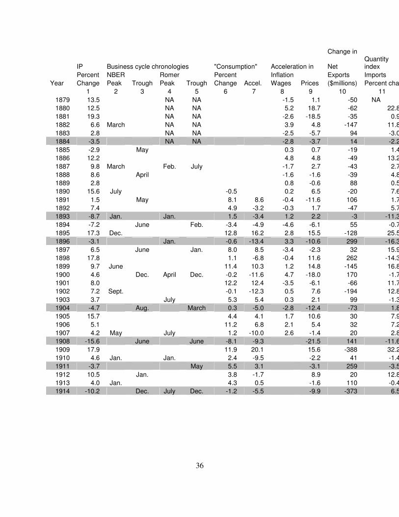
Table 1, column (1) gives percent changes in the Davis index from the previous year. Absolute
declines occurred over 1873-75, 1883-85, 1892-93, 1895-96, 1903-04, 1907-07, 1910-11, and
1913-14. Columns (2) to (5) list months of cyclical peaks and troughs according to the old
NBER chronology and the Romer chronology. All downturns in annual IP are associated with
recessions in both chronologies, except 1883-84. The NBER chronology places a peak in 1882:
this appears to be too early, a case of the inconsistencies noted by Romer. The Romer
chronology cannot cover 1883-84 as the monthly IP index begins in January 1884. The Romer
chronology includes two downturns, in 1887 and 1900, which were too brief to appear in annual
IP; these also appear in the NBER chronology though with slightly different timing. The NBER
chronology includes a downturn in 1890 that appears neither in Romer's chronology nor annual
IP. IP growth slows down sharply from 1890 to 1891, but there is no absolute decline.
If one defines recessions specifically as absolute declines in IP, it still appears that consumption
and inflation were procyclical, and net exports were not. Table 1, column (6) shows the percent
change in Shaw's annual series for the flow of real commodities available for domestic
over time in cyclical “flexibility” (e.g. Cagan 1975, Sachs 1980), but this result was a relic of bad data.

15
consumption (the sum of nondurable, semidurable and durable commodities for household use);
recall this series begins at 1889. Column (7) shows acceleration in consumption – the change in
the growth rate. All downturns in IP were accompanied by slowdowns in consumption growth in
the same year or the prior year. Column (8) shows acceleration in the ECI-style manufacturing
wage index of Hanes (1992). The wage rates constituting the index are from pay periods in the
middle of the summer, so it is not surprising that the slowdown in inflation often appears in the
year following the IP downturn. Column (9) shows acceleration in a WPI constructed from the
standard Warren and Pearson and BLS series but excluding prices of agricultural products. To
match the timing of the wage index, inflation is calculated as the change in the average of
monthly values for June, July and August. The WPI shows the same pattern as the wage index.
Column (10) shows the change in net exports, measured in dollars. This particular series (by
Lipsey 1963), begins with 1879 and gives figures on a calendar-year basis. (Other series go
further back, but are for twelve-month spans ending in June.) Columns (11) and (12) show
percent changes in Lipsey’s calendar-year indexes for real quantities of imports and exports.
There is no clear cyclical pattern in net exports, but imports are clearly procyclical.
Financial Crises
In the pre-1914 gold standard era, America suffered financial crises more frequently than other
countries (Bordo 1985). Most studies of prewar American financial crises (e.g. Sprague 1910,
Wilson, Sylla and Jones 1990, Calomiris and Gorton 1991, Wicker 2000) define them in the
same way, as a general run on banks in New York City, and identify these events objectively by
the actions of the New York Clearing House (NYCH). The NYCH responded to a general run by
issuing clearinghouse loan certificates (Wicker 2000: 116). Using this standard, nearly all studies
say that crises occurred in May 1884; November 1890, May or June 1893, and October 1907
(e.g. Wicker 2000, Calomiris and Gorton 1991). These are the times the NYCH issued
clearinghouse loan certificates. Calomiris and Gorton (1991) identify an additional crisis in
October 1896, when the NYCH authorized certificates but did not issue any. Comparing these
dates with the business-cycle chronologies in Table 1, one can see that nearly all of the crises
occurred during recessions. The crisis of 1890 occurred during a recession according to the old
NBER chronology, but not according to Romer’s or the annual IP series.
16
A panic in New York City was a national crisis because of New York banks’ central role in the
financial system. Loans from New York banks were a key source of funds to nonbank financial
intermediaries (private banks, brokerage houses and commercial-paper houses). New York banks
arranged most loans to firms and individuals who borrowed short-term to finance purchases of
long-term securities (Myers 1931: 265-287, 335) – a particularly obvious form of nonbank
intermediation. On the liability side, New York banks drew interbank deposits – “bankers’
balances” – from all regions of the country. Nearly all banks held deposits in a New York
“correspondent” bank, or in a regional money-center bank that held New York balances (James
1978). An increase in banks’ demand for cash reserves or the nonbank public’s demand for cash
anywhere in the country was ultimately covered by withdrawals of bankers’ balances and
shipments of cash out of New York. Thus, widespread bank runs in the hinterland were quickly
transmitted to New York, while a general run in New York triggered suspensions by other cities’
banks and clearinghouses.
A New York financial crisis must have had real macroeconomic effects that tended to reduce
aggregate output. Because New York bankers’ balances were the chief medium of intercity
payments, a New York run raised real transactions costs of employment and trade as payers
resorted to long-distance cash shipments (James, McAndrews and Weiman 2009). As a run on
New York hindered many types of financial intermediation, it raised the cost of credit and
tightened credit rationing to potential borrowers (Mishkin 1991).
But the timing of financial crises suggests they were not causes of business cycles. Rather, they
amplified cyclical downturns that were already underway. Crises occurred a few months after
cyclical peaks. Calomiris and Gorton (1991) argue that cyclical downturns caused financial
crises: depositors withdrew en masse when they observed or forecast a recession, because a
recession meant defaults on business loans, and this would endanger banks’ solvency. As
evidence, Calomiris and Gorton point out that all crises, without exception, were preceded by
stock-market crashes, which was another symptom indicating the public expected a recession (a
recession would depress corporate earnings). Hanes and Rhode (2011) show that a stock-market
17
crash could actually cause a crisis, because it threatened New York banks’ solvency, or at least
their liquidity. Some New York banks made large unsecured loans to brokerages and other stock
“speculators,” who could not repay in the event of a general decline in stock prices. Depositors
ran on banks rumored to be exposed to stock prices in this way.
A political factor that contributed to the 1884, 1893 and 1896 crises was “silver risk”: the
perceived danger that the U.S. would link the dollar to silver and float against gold. Silver risk
contributed to crises mainly as it reduced international demand for American securities (not by
spurring Americans to withdraw bank deposits for conversion into gold [Sprague, 1910: 165,
169; Friedman and Schwartz, 1963: 108-09]). But silver risk did not trigger the crises. The more-
or-less exogenous political events that created silver risk – the 1878 Bland-Allison Act, the 1890
Sherman Silver Purchase Act – occurred years before the crises in question. Existing research
does not claim that exogenous hikes in silver risk set off crises but rather that potential silver risk
was crystallized by, and amplified, cyclical downturns and financial crises already underway
(Sprague 1910: 109-110, 162, 165, 168, 179, Fels 1959: 130-131, 184-187, Friedman and
Schwartz 1963: 100-101).
Causes of Business Cycles
The cause of a business cycle may be generally defined as an event or combination of events
exogenous to the economic system that is the reason a cyclical downturn occurred in a particular
year. Natural events such as weather and earthquakes are obviously exogenous. For purposes of
understanding American economic history, it can also be useful to treat foreign economic
developments as exogenous.
To establish that a particular event caused a particular business cycle, one must show that the
event occurred with the right timing relative to that business cycle, that events of that type were
generally correlated with fluctuations in aggregate output, and that the correlation reflects
causation from the events to the economy, not the other way around. The last point is often hard
to prove because potential causes of business cycles are rarely as exogenous as earthquakes.
Usually, they might occur for exogenous reasons but also might be responses to economic

18
developments. The best one can do is show that real activity was affected by a proposed causal
event when one can be fairly sure that the event occurred for exogenous reasons; that the event
could be a cause of business cycles in an economic model that depicts a plausible theory; and
that the event was accompanied by other outcomes implied by the model. Thus, as Temin (1998)
points out, claims about causes of business cycles depend on a theoretical framework. Different
theories have different implications as to the type of event that could be responsible for a
downturn and the other outcomes that would, if observed, pin the blame on the suspect. In
macroeconomic theory there is unfortunately little agreement on frameworks. The monumental
study of Friedman and Schwartz (1963) was built on the framework of monetarism. Currently,
most macroeconomic research is in the framework of either Keynesian (“old” and “new”) or
Real Business Cycle (RBC) theory.
In RBC models wages and prices are perfectly flexible, markets clear continuously and all
decision makers are perfectly rational. In standard RBC models the only shock that can generate
the co-movements in output across nonagricultural sectors, consumption, and international trade
that occurred in prewar business cycles is an exogenous, absolute, simultaneous decline in total
factor productivity (TFP) across most sectors of the economy (King and Rebelo 1999).
According to RBC theorists, real events corresponding to a negative TFP shock in an RBC
model include not only deteriorations in production technology per se, but also “changes in the
legal and regulatory system” that impair microeconomic efficiency (Hansen and Prescott 1993:
281). Ebell and Ritschl (2008) and Ohanian (2009) explain the 1929-33 downturn of the Great
Depression this way, as the result of a sudden increase in union bargaining power and Hoover
administration policies that forced employers to pay higher real wages. As far as I know, there
have been no attempts to account for prewar business cycles in terms of RBC models, but I
expect it would be hard to do so. There is no evidence for a general decline in technological or
regulatory efficiency in 1883-84, 1892-93, 1895-96, 1903-04, 1907-08, 1910-11, or 1913-14.
The gold-standard era was notable for a relative absence of government interference in the
economy (Hughes 1991).
In both Keynesian and monetarist models, wages and/or prices are not perfectly flexible. They

19
are “sticky,” subject to nominal rigidity, so that an event affecting aggregate demand can disturb
real activity from the level that would prevail under perfectly flexible wages and prices – the
“natural rate” of output. (Using this definition, output fluctuations in RBC models are
fluctuations in the natural rate.) In most models wage and price stickiness takes the form of the
“expectations-augmented” Phillips curve. In old-fashioned models this is a structural equation
that says inflation is equal to expected inflation plus a positive coefficient times the output gap –
the difference between actual output and the natural rate. In New Keynesian models, an equation
of similar form is derived from “fundamental” assumptions about microeconomic constraints on
price adjustment (e.g. Roberts 1995) or information imperfections (e.g. Mankiw and Reis 2010).4
The apparent change in inflation behavior from the prewar original Phillips curve to the postwar
accelerationist Phillips curve is consistent with an expectations-augmented Phillips curve of
either the old or new-Keynesian variety (Alogoskoufis and Smith 1991, Ball and Mankiw 2002,
Hanes and James 2010). An expectations-augmented Phillips curve generates the prewar pattern
if expected inflation is uncorrelated with past inflation. It generates the postwar pattern if
expected inflation is positively correlated with past inflation. Barsky (1987) shows that, in
postwar samples including the 1970s and 1980s, serial correlation in inflation is so strong that
inflation is statistically indistinguishable from a random walk - that is, current inflation is a good
forecast of future inflation. In pre-1914 data, monthly or annual inflation shows little or no serial
correlation – using standard tests, one cannot reject the hypothesis that the price level was a
random walk. Thus, any roughly rational expectation of inflation would be strongly correlated
with past inflation in the postwar era, uncorrelated with past inflation in the prewar era. The lack
of inflation persistence in the prewar U.S. was an outcome of the monetary regime: under the
gold standard, a country’s aggregate demand growth was subject to a long-term constraint that
did not accommodate persistent inflation (Klein 1975).
The apparent change in the behavior of real consumption wages, from acyclical or
countercyclical prewar to procyclical postwar, is also consistent with nominal rigidity. Hanes
4 Depending on the particular assumptions, the “expected inflation” in the augmented Phillips curve that affects
current inflation may be past expectations of current inflation (as in Mankiw and Reis 2010) or current expectations
of future inflation (Roberts 1995).

20
(1996) and Huang, Liu and Phaneuf (2004) show that real consumption wages become more
procyclical over time if nominal wages are sticky and consumption goods become more finished,
passing through more stages of production and sale prior to purchase by households. Historical
evidence on the nature of consumption bundles shows that consumption goods indeed became
more finished in this sense. In Hanes’ model, more stages make real wages procyclical because
firms’ desired price markups over marginal cost are countercyclical. In the model of Huang, Liu
and Phaneuf it is because wages and prices are both subject to adjustment costs and more stages
make production more roundabout in the sense of Basu (1995).
In the framework of a model with an expectations-augmented Phillips curve, one would say that
the cause of a business-cycle downturn is the exogenous event(s) that causes a large decline in
aggregate demand to occur in a given year. The distinctive monetarist view was that nearly all
fluctuations in aggregate demand were immediately due to changes in the “money stock” – an
aggregate of cash and assets that are relatively close substitutes for cash, such as demand
deposits. Friedman and Schwartz (1963) analyzed the prewar era in this framework, accounting
for money-stock fluctuations in terms of the supply of high-powered money, the fraction of the
money stock the public wants to hold in cash versus deposits, and the fraction of deposits banks
want to hold in cash reserves - the reserve ratio. It is not always clear whether Friedman and
Schwartz view changes in money-stock determinants such as the reserve ratio to be exogenous,
but they do propose a clear, causal explanation of the Depression of 1893. They argue that a
downturn took place in that year because of fluctuations in wheat harvests.
Wheat and wheat flour were important American exports. The size of the wheat harvest had a big
effect on American export revenue. Shocks to export revenue could affect the high-powered
money supply because of the gold standard and America’s lack of a central bank.
Under the gold standard an international flow of monetary gold covered a country’s balance of
payments – the sum of net exports, international capital inflow, and net income from foreign
assets – unless the country's authorities managed stocks of foreign assets. An international flow
of monetary gold affected the high-powered money supply, unless a monetary authority such as a

21
central bank “sterilized” it with an adjustment to the supply of non-gold currency or central-bank
balances. Because the U.S., had no central bank, there was an unusually direct link between the
money supply and the balance of payments. The high-powered money supply consisted of
monetary gold plus non-gold currency issued by the Treasury minus cash held in Treasury vaults
(removed from banks and the public) (Friedman and Schwartz 1963: 124-34). The net inflow of
monetary gold was equal to the balance of payments, as U.S. authorities did not hold stocks of
foreign assets. Non-gold currency growth was unresponsive to economic conditions and mostly
out of the Treasury’s control.5 On occasion, Treasury officials deliberately managed vault cash to
affect the money supply (Myers 1931: 370-86, Timberlake 1978) but they did not generally
sterilize international gold flows.
According to Friedman and Schwartz (1963: 107), the Sherman Silver Purchase Act of 1890
raised fears that the U.S. would leave the gold standard, which tended to reduce the flow of
international investment in the U.S., the balance of payments and hence growth in the high-
powered money supply. But this effect was staved off by a bumper wheat harvest in autumn
1891, an “accident of weather,” coincident with poor harvests abroad. The positive shock to net
exports “fostered a spurt in the stock of money from 1891 to 1892 ... This surcease, however,
was bound to be temporary,” so a downturn occurred in 1893. Wheat export revenues remained
relatively low until a “fortuitous” increase in 1897 which contributed to the 1897 upturn.
A recent study in the monetarist spirit of Friedman and Schwartz is Moen and Tallman (1998),
who examine the relation between the American monetary gold stock and the Miron-Romer
monthly IP index over 1890-1909. They claim that exogenous shocks to gold flow can be
distinguished from endogenous variations (e.g. shocks to American demand for gold) by
regressing the gold stock on IP, short-term interest rates and a few other variables: the residuals
from this regression are the exogenous shocks. (That is, they perform a vector autoregression
[VAR] with the gold stock as one of the variables.) They show that these residual fluctuations in
gold flow were positively related to subsequent growth in IP, and that there were large negative
5 Nongold money consisted of greenbacks, silver notes, national banknotes and silver coins. The quantity of
greenbacks was simply fixed; the rate at which the Treasury created new silver notes was governed by longstanding
22
shocks prior to the downturns of 1893, 1896 and 1907.
In the Keynesian view, the money stock is not the key intermediate factor for aggregate demand;
what matters is the difference between prevailing real interest rates and the “natural rate of
interest,” that is the real interest rate level consistent with the natural rate of output in the IS
curve. In many Keynesian models (e.g. Bernanke, Gertler and Gilchrist 1999) real effects of
interest-rate changes are amplified by their effects on the supply of credit from financial
intermediaries.
Within a Keynesian framework, Davis, Hanes and Rhode (2009) claim that the downturns of
1884, 1893, 1896 and 1910, were caused by fluctuations in cotton harvests. They show that there
was a strong, general positive relation between the size of the cotton harvest and the following
year's IP, within the 1879-1913 gold-standard era specifically, and cotton harvests were
extremely poor in the harvest seasons prior to these downturns (autumn 1883, 1892, 1895 and
1909). To establish the direction of causality, they show that there was an effect from cotton
harvest fluctuations specifically due to weather, an obviously exogenous factor. (That is, they use
weather data to form instruments for harvest fluctuations in two-stage least squares.) Davis,
Hanes and Rhode argue that the apparent effect of cotton harvest fluctuations on IP makes sense
within a Keynesian model, and they show that cotton harvest fluctuations were associated with
other outcomes implied by such a model.
Cotton, like wheat, was an important export. Cotton harvest fluctuations were positively related
to export revenue. Davis, Hanes and Rhode argue that export-revenue shocks affected the
nonagricultural economy because of interactions with the monetary regime, but not through the
money supply. The key intermediate factor was interest rates. American interest rates were
determined by the interaction between the gold standard, net exports, and international capital
flows. International demand for American assets was sensitive (but not infinitely sensitive) to the
spread between expected returns on American versus European assets (as in models of imperfect
international capital mobility). Under the international gold standard, absent a central bank, the
political factors (Myers 1931: 396-398, 402); and the rate at which banks created national bank notes was

23
balance of payments was equal to the change in the high-powered money supply, so the sum of
net exports and capital inflow was constrained by the change in high-powered money demand.
Putting these conditions together, a negative shock to American net exports was balanced either
by an increase in American interest rates, or by an exogenous negative shock to high-powered
money demand. Davis, Hanes and Rhode hypothesize that a poor cotton harvest tended to reduce
American export revenue but had little immediate effect on money demand, while wheat harvest
fluctuations had strong effects on high-powered money demand as well as export revenue. This
implies that during the gold-standard regime specifically, poor cotton harvests would be
associated with higher interest rates, gold outflows and slow high-powered money growth, as
well as a decline in IP. Poor wheat harvests would be associated with gold outflows and slow
money growth but not higher interest rates or lower IP. Davis, Hanes and Rhode show that these
patterns are clear in the data.
In a related paper, Hanes and Rhode (2011) argue that cotton harvests were responsible for the
financial crises of 1884, 1893 and 1896 in the same way, not only by causing business-cycle
downturns but also by reducing international demand for American assets which had a further
effect on stock prices. Their hypothesis implies that poor cotton harvests, but not poor wheat
harvests, tended to drain deposits from New York banks, and depress stock prices and bond
prices prior to IP. These patterns are also clear in the data.
On the same Keynesian argument, monetary tightening by European central banks or other
factors reducing Europeans’ demand for American assets should have affected American
financial markets and real activity like a poor cotton harvest. The financial crisis of 1890, the
financial crisis and cyclical downturn of 1907, and the downturn of 1914 can all be accounted for
in this way.
1890 was the year of the famous Barings Crisis. Events in Argentina depressed prices of
Argentine bonds held by financial intermediaries in London. To raise funds, Barings and other
remarkably insensitive to variations in interest rates and business activity (Myers 1931: 403, Cagan 1965: 91).
24
European financial houses began fire sales of assets including American stocks.6 Meanwhile, a
monetary tightening by the Bank of England raised London bill rates, discouraging American
finance-bill borrowing (Sprague 1910: 133). These conditions caused the 1890 stock-market
crash and financial crisis in New York, according to many contemporaries and modern
economists (e.g. Sprague 1910: 132, Fels 1959: 167, Friedman and Schwartz 1963: 104, Bordo
2006, Reinhart and Rogoff 2009: 243). Hanes and Rhode (2011) argue that they did not cause a
cyclical downturn only because they were largely counteracted by the financial effects of a large
cotton harvest and export revenues in autumn 1890.
The Panic of 1907 followed sharp hikes in European interest rates due to tightening actions by
the Bank of England and other European central banks. In addition to raising its discount rate,
the Bank blocked American borrowing in London with informal threats (Sprague, 1910: 241,
Sayers 1976: 54-56). Friedman and Schwartz (1963: 156) and Eichengreen (1992: 51) identify
these actions as the cause of the 1907 crisis in the U.S. According to Odell and Weidenmier
(2004), European central banks took these actions to counter a persistent international gold drain
caused by payments by European insurance companies associated with the San Francisco
earthquake of April 1906 – an event that took place within the U.S., but may be viewed as
essentially exogenous.
At the end of July 1914, the effects of the First World War's outbreak were initially similar to
1890 and 1907. An increase in European demand for monetary gold and fire sales of American
assets by European investors caused hikes in American interest rates and declines in American
stock and bond prices. But there soon followed unprecedented disruptions to the mechanisms of
international payments and trade finance, demand for American exports, and the closing of the
New York Stock Exchange for more than four months (Sprague 1915, Silber 2006). Because
these disruptions were unprecedented it is hard to quantify their real effects, but it is no surprise
they were accompanied by a business-cycle downturn: July 1914 was a cyclical peak (according
to Romer).
6 Noyes (1898: 157) and Lauck (1907: 64) describe relevant Argentine events. The Economist (Supplement,
February 21, 1891) describes the embarrassments of London financial houses holding Argentine securities; Wilkins
(1989: 194, 222, 471) describes effects of foreign sales of American securities on American financial markets.
25
Conclusion
Deficiencies in historical data may mean the characteristics of prewar business cycles are seen
only as through a glass, darkly, but their causes are surprisingly clear. Within the prewar era
from 1879 to 1914, there were seven recessions big enough to show up as a decline in annual IP:
in 1884, 1893, 1896, 1904, 1907, 1910 and 1914. At least six can be attributed to clearly
exogenous events. 1884, 1893, 1896 and 1910 were caused by poor American cotton crops in the
prior harvest seasons. 1907 was caused by the San Francisco earthquake of 1906. 1914 was
caused by a politically motivated shooting in Sarajevo. All of these events created disturbances
in American financial markets equivalent to exogenous hikes in interest rates, through
mechanisms created by the American gold-standard monetary regime.
26
References
Allen, S. G. (1992) ‘Changes in the cyclical sensitivity of wages in the United States, 1891-
1987,’ American Economic Review, 82: 122-40.
Alogoskoufis, G.S. and Smith, R. (1991) ‘The Phillips curve, the persistence of inflation and the
Lucas critique: evidence from exchange-rate regimes,’ American Economic Review, 81: 1254-75.
Backus, D. K. and Kehoe, P.J. (1992) ‘International evidence on the historical properties of
business cycles,’ American Economic Review, 82: 864-88.
Balke, N.S. and Gordon, R.J. (1989) ‘The estimation of prewar gross national product:
methodology and new evidence,’ Journal of Political Economy, 97: 38-92.
Ball, L. and Mankiw, N.G. (2002) ‘The NAIRU in theory and practice,’ Journal of Economic
Perspectives, 16: 115-36.
Barsky, R.B. (1987) ‘The Fisher effect and the forecastability and persistence of inflation,’
Journal of Monetary Economics 19: 3-24.
Basu, S. (1995) ‘Intermediate goods and business cycles: implications for productivity and
welfare,’ American Economic Review 85: 512-31.
Bernanke, B. S., Gertler, M. and Gilchrist, S. (1999) ‘The financial accelerator in a quantitative
business cycle framework,’ in Taylor, J.B. and Woodford, M. (eds.) Handbook of
Macroeconomics, Amsterdam: Elsevier Science Publications.
Blank, D.M. (1954) The Volume of Residential Construction, 1889-1950, National Bureau of
Economic Research Technical Paper 9.
27
Bordo, M. (1985) ‘The impact and international transmission of financial crises: some historical
evidence, 1870-1933,’ Revista di Storia Economica 2: 41-78.
Bordo, M. (2006) ‘Sudden stops, financial crises and original sin in emerging countries: deja
vu?’ National Bureau of Economic Research Working Paper 12393.
Burns, A.F. (1951) ‘Mitchell on what happens during business cycles,’ in Conference on
Business Cycles, New York: National Bureau of Economic Research.
Cagan, P. (1965) Determinants and Effects of Changes in the Stock of Money, 1875-1960, New
York: Columbia University Press.
Cagan, P. (1975) ‘Changes in the recession behavior of wholesale prices in the 1920s and post-
World War II', Explorations in Economic Research, 2: 54-104.
Calomiris, C.W. and Gorton, G. ‘The origins of banking panics: models, facts and bank
regulation,’ in R.G. Hubbard (ed.) Financial Markets and Financial Crises, Chicago: University
of Chicago Press.
Calomiris, C. W. and Hanes. C. (1994) ‘Consistent output series for the antebellum and
postbellum periods: issues and preliminary results,’ Journal of Economic History, 54: 409-22.
Carter, S.B. and Sutch, R. (1990) ‘The labour market in the 1890s: evidence from Connecticut
Manufacturing,’ in E. Aerts and B. Eichengreen (eds.) Unemployment and Underemployment in
Historical Perspective, Studies in Social and Economic History 12. Leuven: Leuven University
Press.
Carter, S.B., Gartner, S.S., Haines, M.R., Olmstead, A.L., Sutch, R. and Wright, G. (2006)
Historical Statistics of the United States Millennial Edition, New York: Cambridge University
Press.

28
Davis, J.H. (2004) ‘An annual index of U.S. industrial production, 1790-1915,’ Quarterly
Journal of Economics, 119: 1177-1215.
Davis, J.H. (2006) ‘An improved annual chronology of U.S. business cycles,’ Journal of
Economic History, 66: 103-21.
Davis, J.H., Hanes, C. and Rhode, P.W. (2009) ‘Harvests and business cycles in nineteenth-
century America,’ Quarterly Journal of Economics, 124: 1675-1727.
Douglas, P.H. (1930) Real Wages in the United States, 1890-1926, Boston: Houghton Mifflin.
Ebel, M. and Ritschl, A. (2008) ‘Real origins of the Great Depression: monopoly power, unions
and the American business cycle in the 1920s,’ Centre for Economic Performance Discussion
Paper 0876.
Eichengreen, B. (1992) Golden Fetters: The Gold Standard and the Great Depression, 1919-39,
Oxford: Oxford University Press.
Fels, R. (1959) American Business Cycles 1865-1897, Chapel Hill: University of North Carolina
Press.
Frickey, E. (1942) Economic Fluctuations in the United States, Cambridge: Harvard University
Press.
Frickey, E. (1947) Production in the United States 1860-1914, Cambridge: Harvard University
Press.
Friedman, M. and Schwartz, A.J. (1963) A Monetary History of the United States, 1867-1960,
Princeton: Princeton University Press.

29
Gallman, R. E. (1966) ‘Gross national product in the United States, 1834-1909,’ in Studies in
Income and Wealth 30, Output, Employment and Productivity in the United States after 1800,
New York: Columbia University Press..
Gottlieb, M. (1965) ‘New measures of value of nonfarm building for the United States, annually
1850-1939,’ Review of Economics and Statistics, 47: 412-19.
Gordon, R.J. (1990) ‘What is New-Keynesian economics?’ Journal of Economic Literature, 28:
1115-71.
Hanes, C. (1992) ‘Comparable indices of wholesale prices and manufacturing wage rates in the
United States, 1865-1914,’ Research in Economic History, 14: 269-92.
Hanes, C. (1993) ‘The development of nominal wage rigidity in the late 19th century,’ American
Economic Review, 83: 732-56.
Hanes, C. (1996) ‘Changes in the cyclical behavior of real wage rates, 1870-1990,’ Journal of
Economic History, 56: 837-61.
Hanes, C. (1998) ‘Consistent wholesale price series for the United States, 1860-1990,’ in T. Dick
(ed.) Business Cycles Since 1820: New International Perspectives from Historical Evidence,
Cheltenham, UK: Elgar.
Hanes, C. (1999) ‘Degrees of processing and changes in the cyclical behavior of prices in the
United States, 1869-1990,’ Journal of Money, Credit and Banking, 31: 35-53.
Hanes, C. and James, J. (2003) ‘Wage adjustment under low inflation: evidence from U.S.
History,’ American Economic Review, 93: 1414-24.
30
Hanes, C. and James, J. (2010) ‘Wage rigidity in the Great Depression,’ working paper.
Hanes, C. and Rhode, P. W. (2011) ‘Harvests and financial crises in gold-standard America,’
working paper.
Hansen, G.D. and Prescott, E.G. (1993) ‘Did technology shocks cause the 1990-1991 recession?’
American Economic Review, 83: 280-86.
Hoover, E.D. (1960) ‘Retail prices after 1850,’ in Studies in Income and Wealth 24, Trends in
the American Economy in the Nineteenth Century, Princeton: Princeton University Press.
Huang, K.X.D., Liu, Z., and Phaneuf, L. (2004) ‘Why does the cyclical behavior of real wages
change over time?’ American Economic Review, 94: 836-56.
Hughes, J. (1991) The Government Habit Redux: Economic Controls from Colonial Times to the
Present, Princeton: Princeton University Press.
James, J. (1978) Money and Capital Markets in Postbellum America, Princeton: Princeton
University Press.
James, J., McAndrews, J. and Weiman, D.F. (2011) ‘Wall Street and main street: the
macroeconomic consequences of bank suspensions in New York on the national payments
system, 1866 to 1914,’ working paper.
Kendrick, J.W. (1961) Productivity Trends in the United States, Princeton: Princeton University
Press.
Keyssar, A. (1986) Out of Work: The First Century of Unemployment in Massachusetts, New
York: Cambridge University Press.
31
King, R. G. and Rebelo, S.T. (1999) ‘Resuscitating real business cycles,’ in J.B. Taylor and M.
Woddford (eds.) Handbook of Macroeconomics, Amsterdam: Elsevier Science Publications.
Klein, B. (1975) ‘Our new monetary standard: the measurement and effects of price uncertainty,
1880-1973,’ Economic Inquiry, 13: 461-84.
Kuznets, S. S. (1946) National Product since 1869, New York: National Bureau of Economic
Research.
Lauck, W. J. (1907) The Causes of the Panic of 1893, Boston: Houghton-Mifflin.
Lebergott, S. (1964) Manpower in Economic Growth: The American Record Since 1800, New
York: McGraw-Hill.
Lebow, D.E., Saks, R.E. and Wilson, B.A. (2003) ‘Downward nominal wage rigidity: evidence
from the employment cost index,’ Advances in Macroeconomics, 3. Page number?
Lipsey, R.E. (1963) Price and Quantity trends in the Foreign Trade of the United States,
Princeton: Princeton University Press.
Long, C.D. (1960) Wages and Earnings in the United States, 1860-1890, Princeton: Princeton
University Press for National Bureau of Economic Research.
Mankiw, N.G. and Reis, R. (2010) 'Imperfect Information and Aggregate Supply', National
Bureau of Economic Research Working Paper 15773.
Miron, J. A. and Romer, C. D. (1990) 'A New Monthly Index of Industrial Production, 1884-
1940', Journal of Economic History 50: 321-332.
32
Mishkin, F.S. (1991) 'Asymmetric Information and Financial Crises: A Historical Perspective', in
Hubbard, R.G. (ed.) Financial Markets and Financial Crises, Chicago: University of Chicago
for National Bureau of Economic Research.
Meissner, C. (2005) ‘A new world order: explaining the international diffusion of the gold
standard,’ Journal of International Economics, 66: 385-406.
Moen, J. and Tallman, E. (1998) ‘Gold shocks, liquidity, and the United States economy during
the national banking era,’ Explorations in Economic History, 35: 381-404.
Mitchell, W.C. (1951) What Happens During Business Cycles: A Progress Report, New York:
National Bureau of Economic Research.
Myers, M.G. (1931) The New York Money Market, Volume I: Origins and Development, New
York: Columbia University Press.
Noyes, A. D. (1909) Thirty Years of American Finance, New York: G.P. Putnam.
Odell, K.A. and Weidenmier, M. D. (2004) ‘Real shock, monetary aftershock: the 1906 San
Francisco earthquake and the panic of 1907,’ Journal of Economic History, 64: 1002-27.
Ohanian, L. (2009) ‘What - or who - started the Great Depression?’ Journal of Economic Theory,
144: 2310-35.
Phillips, A.W. (1958) ‘The relationship between unemployment and the rate of changes of
money wages in the United Kingdom, 1861-1957,’ Economica, 25: 283-99.
Rees, A. (1961) Real Wages in Manufacturing, 1890-1914, Princeton: Princeton University
Press.

33
Reinhart, C. and Rogoff, K.S. (2009) This Time is Different: Eight Centuries of Financial Folly,
Princeton: Princeton University Press.
Roberts, J.M. (1995) ‘New Keynesian economics and the Phillips curve,’ Journal of Money,
Credit and Banking, 27: 975-84.
Romer, C.D. (1986) ‘Is the stabilization of the postwar economy a figment of the data?’
American Economic Review, 76: 314-34.
Romer, C.D. (1989) ‘The prewar business cycle reconsidered: new estimates of gross national
product, 1869-1908,’ Journal of Political Economy, 97: 1-37.
Romer, C.D. (1991) ‘The cyclical behavior of individual production series, 1889-1984,’
Quarterly Journal of Economics, 106: 1-31.
Romer, C.D. (1994) ‘Remeasuring Business Cycles,’ Journal of Economic History, 54: 573-609.
Sayers, R.S. (1976) The Bank of England, 1891-1944, Cambridge, UK: Cambridge University
Press.
Sachs, J. (1980) ‘The changing cyclical behavior of wages and prices: 1890-1976,’ American
Economic Review, 70: 78-90.
Shaw, W. H. (1947) Value of Commodity Output Since 1869, New York: National Bureau of
Economic Research.
Silber, W.L. (2006) ‘Birth of the Federal Reserve: crisis in the womb,’ Journal of Monetary
Economics, 53: 351-68.
34
Sprague, O.M.W. (1910) History of Crises under the National Banking System, Washington:
Government Printing Office.
Sprague, O.M.W. (1915) ‘The crisis of 1914 in the United States,’ American Economic Review,
5: 499-533.
Temin, P. (1998) ‘The causes of American business cycles: an essay in economic
historiography,’ in J.C. Fuhrer and S. Schuh, (eds.) Beyond Shocks: What Causes Business
Cycles (Federal Reserve Bank of Boston Conference Series 42), Boston: Federal Reserve Bank
of Boston.
Timberlake, R. (1978) The Origins of Central Banking in the United States, Cambridge, MA:
Harvard University Press.
United States Bureau of Economic Analysis (2005), ‘Updated summary NIPA methodologies,’
Survey of Current Business, 85: 11-28.
United States Bureau of the Census (1975), Historical Statistics of the United States Bicentennial
Edition, Washington: Government Printing Office.
Warren, G.F. and F.A. Pearson (1932) Wholesale Prices for 213 Years, 1720 to 1932, Ithaca,
NY: Cornell University Agricultural Experiment Station Memoir 142.
Watson, M.W. (1994) ‘Business-cycle durations and postwar stabilization of the U.S. economy,’
American Economic Review, 84: 24-46.
Weir, D. R. (1992), ‘A century of U.S. unemployment, 1890-1990: revised estimates,’ Research
in Economic History, 14: 301-46.
Wicker, E. (2000) Banking Panics of the Gilded Age, Cambridge: Cambridge University Press.

35
Wilkins, M. (1989) The History of Foreign Investment in the United States to 1914, Cambridge,
MA: Harvard University Press.
Wilson, J.W., Sylla, R.E. and Jones, C.P. (1990) ‘Financial market panics and volatility in the
long run, 1830-1988,’ in E. White (ed.) Crashes and Panics: The Lessons from History,
Homewood, IL: Dow Jones-Irwin.
36
Change in
IP Business cycle chronologies "Consumption" Acceleration in Net Quantity index
Percent NBER Romer Percent Inflation Exports Imports
Year Change Peak Trough Peak Trough Change Accel. Wages Prices ($millions) Percent change
1 2 3 4 5 6 7 8 9 10 11
1879 13.5 NA NA -1.5 1.1 -50 NA
1880 12.5 NA NA 5.2 18.7 -62 22.8
1881 19.3 NA NA -2.6 -18.5 -35 0.9
1882 6.6 March NA NA 3.9 4.8 -147 11.8
1883 2.8 NA NA -2.5 -5.7 94 -3.0
1884 -3.5 NA NA -2.8 -3.7 14 -2.2
1885 -2.9 May 0.3 0.7 -19 1.4
1886 12.2 4.8 4.8 -49 13.2
1887 9.8 March Feb. July -1.7 2.7 -43 2.7
1888 8.6 April -1.6 -1.6 -39 4.8
1889 2.8 0.8 -0.6 88 0.5
1890 15.6 July -0.5 0.2 6.5 -20 7.6
1891 1.5 May 8.1 8.6 -0.4 -11.6 106 1.7
1892 7.4 4.9 -3.2 -0.3 1.7 -47 5.7
1893 -8.7 Jan. Jan. 1.5 -3.4 1.2 2.2 -3 -11.3
1894 -7.2 June Feb. -3.4 -4.9 -4.6 -6.1 55 -0.7
1895 17.3 Dec. 12.8 16.2 2.8 15.5 -128 25.5
1896 -3.1 Jan. -0.6 -13.4 3.3 -10.6 299 -16.3
1897 6.5 June Jan. 8.0 8.5 -3.4 -2.3 32 15.9
1898 17.8 1.1 -6.8 -0.4 11.6 262 -14.3
1899 9.7 June 11.4 10.3 1.2 14.8 -145 16.8
1900 4.6 Dec. April Dec. -0.2 -11.6 4.7 -18.0 170 -1.7
1901 8.0 12.2 12.4 -3.5 -6.1 -66 11.7
1902 7.2 Sept. -0.1 -12.3 0.5 7.6 -194 12.8
1903 3.7 July 5.3 5.4 0.3 2.1 99 -1.3
1904 -4.7 Aug. March 0.3 -5.0 -2.8 -12.4 -73 1.8
1905 15.7 4.4 4.1 1.7 10.6 30 7.9
1906 5.1 11.2 6.8 2.1 5.4 32 7.2
1907 4.2 May July 1.2 -10.0 2.6 -1.4 20 2.8
1908 -15.6 June June -8.1 -9.3 -21.5 141 -11.6
1909 17.9 11.9 20.1 15.6 -388 32.2
1910 4.6 Jan. Jan. 2.4 -9.5 -2.2 41 -1.4
1911 -3.7 May 5.5 3.1 -3.1 259 -3.5
1912 10.5 Jan. 3.8 -1.7 8.9 20 12.8
1913 4.0 Jan. 4.3 0.5 -1.6 110 -0.4
1914 -10.2 Dec. July Dec. -1.2 -5.5 -9.9 -373 6.5
Recommended