c© 2012 Chia-Lun Chang

OBSERVING LIMITATIONS OF THE DISCRETE HILBERTTRANSFORM WITH S-PARAMETER MEASUREMENTS OF
MICROSTRIPS AND STRIPLINES
BY
CHIA-LUN CHANG
THESIS
Submitted in partial fulfillment of the requirementsfor the degree of Master of Science in Electrical and Computer Engineering
in the Graduate College of theUniversity of Illinois at Urbana-Champaign, 2012
Urbana, Illinois
Adviser:
Professor Jose E. Schutt-Aine

ABSTRACT
S-parameter measurements of microstrips and striplines were done. The
physical properties of the devices under test, consisting of nine single copla-
nar traces and nine pairs of coupled coplanar traces, are provided. The lab
setup and equipment used to make such measurements are explained along
with labeled pictures for visualization. Next, with the measured data, the
limitations of the discrete Hilbert transform were tested. The results show
the kind of properties frequency response data should have in order for the
discrete Hilbert transform to correctly determine whether the data is causal
or not.
ii

To my parents, for their love and support
iii

ACKNOWLEDGMENTS
I would like to express my thanks to my research adviser, Professor Jose
Schutt-Aine, for his continual guidance over the last two years. Thanks also
go to Subramanian Lalgudi for his opinions and technical insights regarding
the discrete Hilbert transform, Jilin Tan from Cadence for providing the
physical board and board description file, Dmitri Klokotov who helped me
numerous times with organizing the lab setup in room 450C, Dan Mast from
the parts shop for advice on different equipment, and Scott McDonald from
the machine shop for fixing the vibration isolation table and improving the
nitrogen tank setup. My officemates Patrick Goh, Tom Comberiate, and Si
Win provided ideas and feedback throughout my stay.
iv

TABLE OF CONTENTS
CHAPTER 1 INTRODUCTION . . . . . . . . . . . . . . . . . . . . 1
CHAPTER 2 BOARD AND TRACE DESCRIPTIONS . . . . . . . . 22.1 General Board Descriptions . . . . . . . . . . . . . . . . . . . 22.2 Single Coplanar Traces . . . . . . . . . . . . . . . . . . . . . . 52.3 Coupled Coplanar Traces . . . . . . . . . . . . . . . . . . . . . 8
CHAPTER 3 MEASUREMENT PROCEDURE . . . . . . . . . . . . 133.1 Vibration Isolation Table . . . . . . . . . . . . . . . . . . . . . 133.2 Measurement Setup . . . . . . . . . . . . . . . . . . . . . . . . 153.3 Calibration . . . . . . . . . . . . . . . . . . . . . . . . . . . . 213.4 Handling the Data . . . . . . . . . . . . . . . . . . . . . . . . 223.5 Results . . . . . . . . . . . . . . . . . . . . . . . . . . . . . . . 23
CHAPTER 4 CHECKING FOR CAUSALITY . . . . . . . . . . . . . 354.1 Background . . . . . . . . . . . . . . . . . . . . . . . . . . . . 354.2 Discrete Hilbert Transform . . . . . . . . . . . . . . . . . . . . 364.3 Sampling Theorem . . . . . . . . . . . . . . . . . . . . . . . . 374.4 Results . . . . . . . . . . . . . . . . . . . . . . . . . . . . . . . 37
CHAPTER 5 CONCLUSIONS . . . . . . . . . . . . . . . . . . . . . 58
REFERENCES . . . . . . . . . . . . . . . . . . . . . . . . . . . . . . . 59
v

CHAPTER 1
INTRODUCTION
Actual S-parameter measurements of microstrips and striplines with their
physical properties extensively documented are valuable. The data will pro-
vide different test cases for researchers in the area of signal integrity sim-
ulations and electromagnetic field solvers to benchmark their codes with.
Measured data would be a lot more reliable than data generated from elec-
tronic design automation (EDA) tools since it is up to the researchers in
the related fields to come up with new algorithms for improving software.
Generated data will not properly account for problems that motivate the
researchers to develop newer simulation techniques in the first place.
One such ongoing problem is causality of physical systems. The real and
imaginary parts of the frequency response are not independent of each other
[1]. Checking for causality has been an active research area with multiple
proposals on how to properly verify the relationship between the real and
imaginary part of the frequency response [2]–[4], and one of them is known
as the discrete Hilbert transform [5]. The effectiveness of the discrete Hilbert
transform along with its limitations as to when it would fail will be investi-
gated.
1
CHAPTER 2
BOARD AND TRACE DESCRIPTIONS
The FR-4 board along with the associated ems3d R12 nets.brd file describing
the board were both provided by Cadence. The Allegro Free Physical Viewer
software from the Cadence website [6] can be downloaded by going through
Products → PCB Design → Allegro Downloads and making sure that it is
compatible with version 16.4. Images shown in this thesis are from Allegro
Free Physical Viewer 16.5.
2.1 General Board Descriptions
Press F10 or click on the Grid Toggle button to remove the default grid
points if preferable. The option to change units for length may be located
by going to Setup → Design Parameters... and click on the Design tab at
the top. The default units is in mils. Distance between two points may be
measured by using the Display → Measure or Shift+F4 option. Clicking on
any subsequent two points will pop up a window with information about
their distance. Similarly, the Display→ Constraint option allows the user to
identify the air gap distance between two Nets. The Measure and Constraint
features are useful for keeping track of the exact geometries and layout of
the traces being measured. The aforementioned features are also helpful in
determining the dimensions of the probes needed in order to measure the
different DUTs on the board. Nets and Vias may be identified by starting
with the Display → Element or F4 option. Then hover over the Find tab
to the right and check the objects of interest such as Nets and Vias. Now
hovering the cursor back to the different parts of the board will highlight the
names of the Nets and Vias.
Different layers may be shown or hidden by hovering over the Visibility tab
on the right and selecting the different All checkboxes beside each respective
2

layer. The properties of the different layers within the board may be found
under Setup → Cross-section... The details are listed in Tables 2.1, 2.2 and
2.3. Note that not all of the layers listed are present for the nine single single
traces and nine coupled traces that were measured. The exact trace by trace
descriptions with the different layers will be documented in their relevant
sections.
Table 2.1: Layer properties 1
Subclass Name Type MaterialAIR ABOVE SURFACE AIR
TOP CONDUCTOR COPPERHDI DIELECTRIC DIELECTRIC FR-4
SIGNAL 2 CONDUCTOR COPPERPREPREG T DIELECTRIC FR-4
SIGNAL 3 PLANE COPPERCORE DIELECTRIC FR-4
SIGNAL 4 PLANE COPPERPREPREG B DIELECTRIC FR-4
SIGNAL 5 CONDUCTOR COPPERHDI VIA FILL DIELECTRIC FR-4
BOTTOM CONDUCTOR COPPERAIR BELOW SURFACE AIR
Table 2.2: Layer properties 2
Subclass Name Thickness (MIL) Conductivity(mho/cm)AIR ABOVE 0
TOP 0.6 595900HDI DIELECTRIC 3.7 0
SIGNAL 2 0.6 595900PREPREG T 3 0
SIGNAL 3 0.6 595900CORE 28 0
SIGNAL 4 0.6 595900PREPREG B 3 0
SIGNAL 5 0.6 595900HDI VIA FILL 3.7 0
BOTTOM 0.6 595900AIR BELOW 0
3

Table 2.3: Layer properties 3
Subclass Name Dielectric Constant Loss TangentAIR ABOVE 1 0
TOP 4.5 0HDI DIELECTRIC 4.5 0.035
SIGNAL 2 4.5 0.035PREPREG T 4.5 0.035
SIGNAL 3 4.5 0.035CORE 4.5 0.035
SIGNAL 4 4.5 0.035PREPREG B 4.5 0.035
SIGNAL 5 4.5 0.035HDI VIA FILL 4.5 0.035
BOTTOM 4.5 0AIR BELOW 1 0
4

2.2 Single Coplanar Traces
2.2.1 General Conventions
Figure 2.1: Single traces convention
Three different S-parameter measurements were made for each single copla-
nar traces for a total of 27 files. The file name conventions are given below
with Figure 2.1 showing the corresponding probe locations.
• TOP represents 1-port reflection with a probe at the top.
• BOTTOM represents 1-port reflection with a probe at the bottom.
• Just the net name by itself represents 2-port S parameters with probes
at both the top and bottom.
2.2.2 Trace by Trace Descriptions
A total of nine single coplanar traces were measured. Each trace has a length
of 1000mils with a width of 5mils. The pitch between the ground and signal
traces is 250µm. SIGNAL 2, SIGNAL 3 and SIGNAL 5 ground planes are
present and underneath all nine traces.
5

Figure 2.2: Single traces 1
Figure 2.3: Single traces 2
6

Figure 2.4: Single traces 3
• N11 from Figure 2.2: Microstrip with large auxiliary ground plane
surrounding signal trace on the TOP layer. The auxiliary ground was
kept floating and is 145mils wide on both sides. The air gap between
the auxiliary ground to the signal trace is 5mils on both sides.
• N10 from Figure 2.2: Microstrip with large ground plane surrounding
signal trace on the TOP layer. Ground is 145mils wide on both sides.
The air gap between ground to the signal trace is 5mils on both sides.
• N9 from Figure 2.2: Microstrip with large ground plane surrounding
signal trace on the TOP layer with multiple ground vias through the
ground planes. Ground is 145mils wide on both sides. The air gap
between ground to the signal trace is 5mils on both sides.
• N3 from Figure 2.3: Microstrip with small auxiliary ground plane sur-
rounding signal trace on the TOP layer. The auxiliary ground was
kept floating and is 30mils wide on both sides. The air gap between
the auxiliary ground to the signal trace is 5mils on both sides.
• N2 from Figure 2.3: Microstrip with small ground plane surrounding
signal trace on the TOP layer. Ground is 30mils wide on both sides.
The air gap between ground to the signal trace is 5mils on both sides.
7

• N1 from Figure 2.3: Microstrip with small ground plane surrounding
signal trace on the TOP layer with multiple ground vias through the
ground planes. Ground is 30mils wide on both sides. The air gap
between ground to the signal trace is 5mils on both sides.
• N13 from Figure 2.4: Stripline with large auxiliary ground plane sur-
rounding signal trace on the SIGNAL 4 layer. The auxiliary ground
was kept floating and is 145mils wide on both sides. The air gap be-
tween the auxiliary ground to the signal trace is 5mils on both sides.
• N14 from Figure 2.4: Stripline with large ground plane surrounding
signal trace on the SIGNAL 4 layer. Ground is 145mils wide on both
sides. The air gap between ground to the signal trace is 5mils on both
sides.
• N15 from Figure 2.4: Stripline with large ground plane surrounding
signal trace on the SIGNAL 4 layer with multiple ground vias through
the ground planes. Ground is 145mils wide on both sides. The air gap
between ground to the signal trace is 5mils on both sides.
2.3 Coupled Coplanar Traces
2.3.1 General Conventions
Ten different S-parameter measurements were made for each coupled copla-
nar traces for a total of 90 files. The file name conventions are given below
with Figure 2.5 showing the corresponding probe locations.
• A represents 1-port reflection with a probe at A.
• B represents 1-port reflection with a probe at B.
• C represents 1-port reflection with a probe at C.
• D represents 1-port reflection with a probe at D.
• AB represents 2-port S parameters with probes at both A and B.
• AC represents 2-port S parameters with probes at both A and C.
8
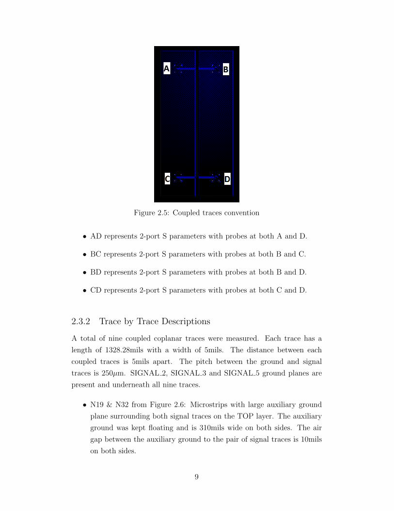
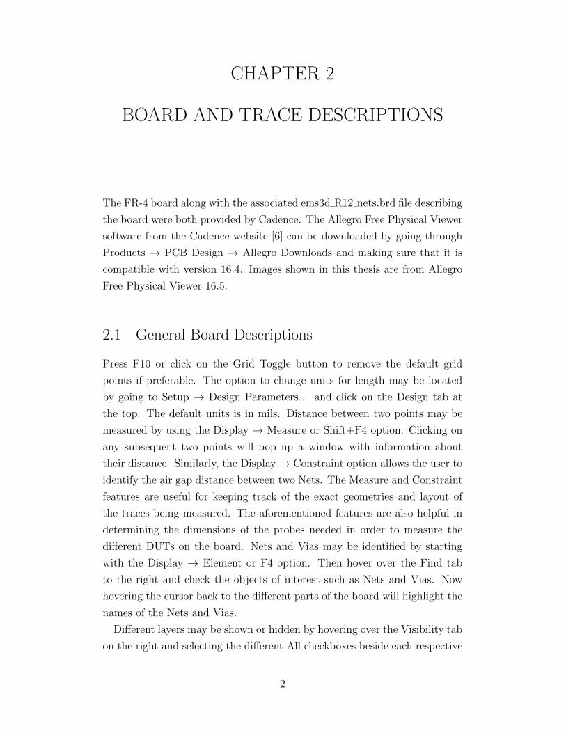
Figure 2.5: Coupled traces convention
• AD represents 2-port S parameters with probes at both A and D.
• BC represents 2-port S parameters with probes at both B and C.
• BD represents 2-port S parameters with probes at both B and D.
• CD represents 2-port S parameters with probes at both C and D.
2.3.2 Trace by Trace Descriptions
A total of nine coupled coplanar traces were measured. Each trace has a
length of 1328.28mils with a width of 5mils. The distance between each
coupled traces is 5mils apart. The pitch between the ground and signal
traces is 250µm. SIGNAL 2, SIGNAL 3 and SIGNAL 5 ground planes are
present and underneath all nine traces.
• N19 & N32 from Figure 2.6: Microstrips with large auxiliary ground
plane surrounding both signal traces on the TOP layer. The auxiliary
ground was kept floating and is 310mils wide on both sides. The air
gap between the auxiliary ground to the pair of signal traces is 10mils
on both sides.
9

Figure 2.6: Coupled traces 1
Figure 2.7: Coupled traces 2
10

Figure 2.8: Coupled traces 3
• N33 & N34 from Figure 2.6: Microstrips with large ground plane sur-
rounding both signal traces on the TOP layer. Ground is 310mils wide
on both sides. The air gap between ground to the pair of signal traces
is 5mils on both sides.
• N35 & N36 from Figure 2.6: Microstrips with large ground plane sur-
rounding both signal traces on the TOP layer with multiple ground
vias through the ground planes. Ground is 310mils wide on both sides.
The air gap between ground to the pair of signal traces is 5mils on both
sides.
• N26 & N38 from Figure 2.7: Microstrips with small auxiliary ground
plane surrounding both signal traces on the TOP layer. The auxiliary
ground was kept floating and is 30mils wide on both sides. The air gap
between the auxiliary ground to the pair of signal traces is 5mils on
both sides.
• N27 & N28 from Figure 2.7: Microstrips with small ground plane sur-
rounding both signal traces on the TOP layer. Ground is 30mils wide
on both sides. The air gap between ground to the pair of signal traces
is 5mils on both sides.
11

• N29 & N30 from Figure 2.7: Microstrips with small ground plane sur-
rounding both signal traces on the TOP layer with multiple ground
vias through the ground planes. Ground is 30mils wide on both sides.
The air gap between ground to the pair of signal traces is 5mils on both
sides.
• N20 & N21 from Figure 2.8: Striplines with large auxiliary ground plane
surrounding both signal traces on the SIGNAL 4 layer. The auxiliary
ground was kept floating and is 310mils wide on both sides. The air
gap between the auxiliary ground to the pair of signal traces is 10mils
on both sides.
• N22 & N23 from Figure 2.8: Striplines with large ground plane sur-
rounding both signal traces on the SIGNAL 4 layer. Ground is 310mils
wide on both sides. The air gap between ground to the pair of signal
traces is 10mils on both sides.
• N24 & N25 from Figure 2.8: Striplines with large ground plane sur-
rounding both signal traces on the SIGNAL 4 layer with multiple ground
vias through the ground planes. Ground is 310mils wide on both sides.
The air gap between ground to the pair of signal traces is 5mils on both
sides.
12

CHAPTER 3
MEASUREMENT PROCEDURE
3.1 Vibration Isolation Table
Figure 3.1: Nitrogen tank with labeled parts to read from and adjust
S-parameter measurements may be made with the probe station on top of
a vibration isolation table. As shown in Figure 3.1, turn on the main valve of
the compressed nitrogen tank and adjust the general purpose regulator knob
to set the pressure to around 40psi. As shown in Figure 3.2, make sure to
tune the knob underneath the vibration isolation table such that it is set to
about 40psi as well. Wait for a few minutes until the tabletop starts to stay
afloat. As shown in Figure 3.3, tune the screws from the three adjustable
corners of the vibration isolation table to make sure that the tabletop is level.
Adjust the general purpose regulator knob to set it back down to 0psi and
turn off the main valve of the compressed nitrogen tank when measurements
are done.
13

Figure 3.2: Knob and meter under vibration isolation table
Figure 3.3: One of three screws to adjust level of tabletop
14
3.2 Measurement Setup
Figure 3.4: Cascade Microtech 250µm pitch GSG probes
Figure 3.5: A pair of 3.5mm female to 3.5mm male with 90 degree bendcables for connecting GSG probes to network analyzer
A pair of Cascade Microtech 250µm Ground-Signal-Ground (GSG) probes
[7] were used as shown in Figure 3.4. A pair of 3.5mm female to 3.5mm
male with 90 degree bend cables as shown in Figure 3.5 are necessary or
15

Figure 3.6: A few tools to help with measurement setup
else the cables going from the probes to the network analyzer would not
fit the probe station setup. Adapters going from type N to 3.5mm are
needed for the E8358A network analyzer since the instrument only goes up
to 9GHz. Adapters going from 2.4mm to 3.5mm are needed for the E8363B
and HP8510C network analyzers since the instruments can go up to 40GHz
and 50GHz, respectively.
A few tools to help with the measurement setup are shown in Figure 3.6.
Their uses are:
• A: for tightening 3.5mm connectors.
• B: for tightening 2.4mm connectors.
• C: for fastening screws to secure probes on the probe bases.
• D: for fastening screws to secure probe bases onto the probe station.
The different parts at the upper half of the probe station setup are shown
in Figure 3.7. They are:
• A: knob for zooming in and out.
• B: switch to flip between looking at the DUT from the probe station
directly, or from the computer with a BNC to BNC cable connected to
16

Figure 3.7: Upper half of probe station
Figure 3.8: Lower half of probe station
17

the video camera on the probe station. Use HDTV2000 software for
the latter option.
• C: knob to set the focus, must be adjusted whenever the distance be-
tween the DUT and the lens changes.
• D: knob to move the lens to view different parts of the DUT. Especially
helpful when probes have landed.
The different parts at the lower half of the probe station setup are shown
in Figure 3.8. They are
• A: platform where the probe bases are placed. The platform needs
to be repositioned when switching from AB, and CD coupled traces
measurements to AC, AD, BC, and BD coupled traces measurements.
The adjustment is needed since the range a probe may move around at
a particular probe station position is limited.
• B: lever to raise or lower the platform in A.
• C: large screw for adjusting the height of the platform where DUTs are
placed. Should not be used when probes have landed.
• D: knob to adjust the orientation of the platform where DUTs are
placed. Used to make sure the three GSG tips from both probes align
with the GSG traces on the DUTs. Should not be used when probes
have landed.
• E: knob to adjust the location of the platform where DUTs are placed
vertically. Should not be used when probes have landed.
• F: knob to adjust the location of the platform where DUTs are placed
horizontally. Should not be used when probes have landed.
An air pump as shown in Figure 3.9 is needed to make sure the DUT would
not move around during measurements. Flip on the appropriate vacuum
switches on the side of the probe station based on how large the DUTs
are. The switches are shown in Figure 3.10. The third switch is flipped
when probing the CS-5 calibration substrate. All switches were flipped when
probing the board provided by Cadence.
18

Figure 3.9: Air pump used to provide vacuum to hold DUTs in place
Figure 3.10: Vacuum switches on the side of the probe station
19

Figure 3.11: Cadence board with measured DUTs marked by the rectangles
20

The actual Cadence board is shown in Figure 3.11. Going row by row and
from left to right,
• First rectangular box corresponds to traces in Figure 2.2.
• Second rectangular box: corresponds to traces in Figure 2.3.
• Third rectangular box: corresponds to traces in Figure 2.6.
• Fourth rectangular box: corresponds to traces in Figure 2.7.
• Fifth rectangular box: corresponds to traces in Figure 2.4.
• Sixth rectangular box: corresponds to traces in Figure 2.8.
3.3 Calibration
Figure 3.12: CS-5 calibration standards from GGB
A preliminary measurement with the HP8510C Network Analyzer was
made with a start frequency of 50MHz and a stop frequency of 40GHz with
21
a total of 801 evenly spaced frequency points. Two additional sets of mea-
surements were then made to cover a slightly wider bandwidth to get data
closer to DC. Agilent E8358A PNA Network Analyzer was set to a start fre-
quency of 300kHz and a stop frequency of 9GHz with a total of 801 evenly
spaced frequency points. Agilent E8363B PNA Network Analyzer was set
to a start frequency of 10MHz and a stop frequency of 40GHz with a to-
tal of 801 evenly spaced frequency points. The three sets of measurements
made with the different network analyzers all used the Short Open Line
Through (SOLT) calibration with the CS-5 calibration substrate made from
GGB [8]. The CS-5 calibration substrate is shown in Figure 3.12. Load the
CK CS525.0 calibration file for the HP8510C network analyzer. Load the
CS-5 250.ckt calibration file for the E8358A and E8363B network analyzers.
Both files may be requested by emailing GGB the name of the calibration
substrate, the model of the network analyzer, and the type of probes being
used.
The corresponding row of CS-5 standards used to calibrate the reference
plane to the tips of the probes are:
• S: row of short standards.
• O: row of open standards.
• M: row of load standards.
• L1: row of through standards.
3.4 Handling the Data
Both Agilent E8358A and Agilent E8363B are capable of saving directly into
.s2p files. As for the HP8510C, it is connected to the computer with GPIB
cables so data may be imported directly to Advanced Design Systems (ADS)
2011.
Start by creating or loading a Workspace in ADS 2011, then open up a new
schematic by going to Window → New Schematic. Next go through Tools
→ Instrument Server... to bring up an user interface to send commands and
receive data from the network analyzer remotely. From the top, select HP-
IB → Symbolic Name and type in gpib0 and click Ok. This will establish a
22

connection between the computer and the HP8510C. Make sure to select the
Network Analyzer option and input in the appropriate HPIB Address of the
HP8510C. Type in an appropriate string for Dataset Name and click Read
Instrument at the bottom left with the Formatted option selected at the top
right along with the ALL S PARAMETERS option right below it.
To view the imported data, go to Window → New Data Display to access
all sorts of plotting features. Go to Tools → Data File Tool... and select
Write data file from dataset at the top. Provide a name along with where
the .s2p file should be saved. Select Touchstone file format and any sort
of conventions on how the S-parameter data should be saved. Locate the
Dataset name to export out as a .s2p file and click Write To File at the
bottom left. This will generate the equivalent .s2p file which could then be
read in and processed by MATLAB.
A MATLAB function called mhdrload [9] was used to help import in the
saved .s2p files into the workspace. The mhdrload function will separate
header information and actual data and import them as separate variables.
3.5 Results
The 300kHz string represents the data measured from 300kHz to 9GHz with
801 frequency points with the Agilent E8358A PNA Network Analyzer. The
10MHz string represents the data measured from 10MHz to 40GHz with 801
frequency points with the Agilent E8363B PNA Network Analyzer.
The impulse responses of the 18 sets of S-parameter measurements from
10MHz to 40GHz are shown in Figures 3.13 to 3.30. The 10MHz data point
was assumed to be the DC point in order to take the inverse fast Fourier
transform with the ifft function in MATLAB. The times of the first peaks
were marked so comparisons may be made between the different traces based
on their physical dimensions.
23
0 0.5 1 1.5 2 2.5
x 10−8
0
0.05
0.1
0.15
0.2
0.25
0.3
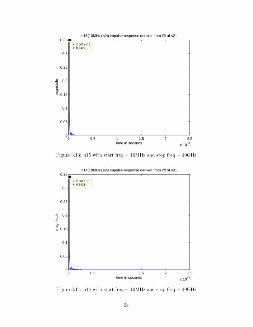
0.35X: 2.002e−10Y: 0.3496
n15(10MHz).s2p impulse response derived from ifft of s21
time in seconds
mag
nitu
de
Figure 3.13: n15 with start freq = 10MHz and stop freq = 40GHz
0 0.5 1 1.5 2 2.5
x 10−8
0
0.05
0.1
0.15
0.2
0.25
0.3
0.35
X: 2.002e−10Y: 0.3411
n14(10MHz).s2p impulse response derived from ifft of s21
time in seconds
mag
nitu
de
Figure 3.14: n14 with start freq = 10MHz and stop freq = 40GHz
24

0 0.5 1 1.5 2 2.5
x 10−8
0
0.05
0.1
0.15
0.2
0.25
0.3
0.35
X: 2.002e−10Y: 0.3201
n13_float(10MHz).s2p impulse response derived from ifft of s21
time in seconds
mag
nitu
de
Figure 3.15: n13 with start freq = 10MHz and stop freq = 40GHz
0 0.5 1 1.5 2 2.5
x 10−8
0
0.05
0.1
0.15
0.2
0.25
0.3
0.35
0.4
0.45
X: 1.501e−10Y: 0.4227
n9(10MHz).s2p impulse response derived from ifft of s21
time in seconds
mag
nitu
de
Figure 3.16: n9 with start freq = 10MHz and stop freq = 40GHz
25

0 0.5 1 1.5 2 2.5
x 10−8
0
0.05
0.1
0.15
0.2
0.25
0.3
0.35
0.4
0.45
X: 1.626e−10Y: 0.4291
n10(10MHz).s2p impulse response derived from ifft of s21
time in seconds
mag
nitu
de
Figure 3.17: n10 with start freq = 10MHz and stop freq = 40GHz
0 0.5 1 1.5 2 2.5
x 10−8
0
0.05
0.1
0.15
0.2
0.25
0.3
0.35
0.4
0.45
X: 1.626e−10Y: 0.401
n11_float(10MHz).s2p impulse response derived from ifft of s21
time in seconds
mag
nitu
de
Figure 3.18: n11 with start freq = 10MHz and stop freq = 40GHz
26

0 0.5 1 1.5 2 2.5
x 10−8
0
0.05
0.1
0.15
0.2
0.25
0.3
0.35
0.4
0.45
X: 1.626e−10Y: 0.4079
n1(10MHz).s2p impulse response derived from ifft of s21
time in seconds
mag
nitu
de
Figure 3.19: n1 with start freq = 10MHz and stop freq = 40GHz
0 0.5 1 1.5 2 2.5
x 10−8
0
0.05
0.1
0.15
0.2
0.25
0.3
0.35
0.4
0.45
X: 1.501e−10Y: 0.4398
n2(10MHz).s2p impulse response derived from ifft of s21
time in seconds
mag
nitu
de
Figure 3.20: n2 with start freq = 10MHz and stop freq = 40GHz
27

0 0.5 1 1.5 2 2.5
x 10−8
0
0.05
0.1
0.15
0.2
0.25
0.3
0.35
0.4
0.45
X: 1.626e−10Y: 0.4295
n3_float(10MHz).s2p impulse response derived from ifft of s21
time in seconds
mag
nitu
de
Figure 3.21: n3 with start freq = 10MHz and stop freq = 40GHz
0 0.5 1 1.5 2 2.5
x 10−8
0
0.05
0.1
0.15
0.2
0.25
0.3
0.35
X: 2.627e−10Y: 0.3114
n24_n25_ac(10MHz).s2p impulse response derived from ifft of s21
time in seconds
mag
nitu
de
Figure 3.22: n24 n25 ac with start freq = 10MHz and stop freq = 40GHz
28

0 0.5 1 1.5 2 2.5
x 10−8
0
0.05
0.1
0.15
0.2
0.25
0.3
0.35
X: 2.502e−10Y: 0.3301
n22_n23_ac(10MHz).s2p impulse response derived from ifft of s21
time in seconds
mag
nitu
de
Figure 3.23: n22 n23 ac with start freq = 10MHz and stop freq = 40GHz
0 0.5 1 1.5 2 2.5
x 10−8
0
0.05
0.1
0.15
0.2
0.25
0.3
0.35
X: 2.502e−10Y: 0.3361
n20_n21_float_ac(10MHz).s2p impulse response derived from ifft of s21
time in seconds
mag
nitu
de
Figure 3.24: n20 n21 float ac with start freq = 10MHz and stop freq =40GHz
29

0 0.5 1 1.5 2 2.5
x 10−8
0
0.05
0.1
0.15
0.2
0.25
0.3
0.35
0.4
X: 2.127e−10Y: 0.389
n35_n36_ac(10MHz).s2p impulse response derived from ifft of s21
time in seconds
mag
nitu
de
Figure 3.25: n35 n36 ac with start freq = 10MHz and stop freq = 40GHz
0 0.5 1 1.5 2 2.5
x 10−8
0
0.05
0.1
0.15
0.2
0.25
0.3
0.35
0.4
X: 2.127e−10Y: 0.3735
n33_n34_ac(10MHz).s2p impulse response derived from ifft of s21
time in seconds
mag
nitu
de
Figure 3.26: n33 n34 ac with start freq = 10MHz and stop freq = 40GHz
30

0 0.5 1 1.5 2 2.5
x 10−8
0
0.05
0.1
0.15
0.2
0.25
0.3
0.35
X: 2.127e−10Y: 0.3421
n19_n32_float_ac(10MHz).s2p impulse response derived from ifft of s21
time in seconds
mag
nitu
de
Figure 3.27: n19 n32 float ac with start freq = 10MHz and stop freq =40GHz
0 0.5 1 1.5 2 2.5
x 10−8
0
0.05
0.1
0.15
0.2
0.25
0.3
0.35
0.4
X: 2.002e−10Y: 0.3941
n29_n30_ac(10MHz).s2p impulse response derived from ifft of s21
time in seconds
mag
nitu
de
Figure 3.28: n29 n30 ac with start freq = 10MHz and stop freq = 40GHz
31

0 0.5 1 1.5 2 2.5
x 10−8
0
0.05
0.1
0.15
0.2
0.25
0.3
0.35
0.4
X: 2.002e−10Y: 0.3575
n27_n28_ac(10MHz).s2p impulse response derived from ifft of s21
time in seconds
mag
nitu
de
Figure 3.29: n27 n28 ac with start freq = 10MHz and stop freq = 40GHz
0 0.5 1 1.5 2 2.5
x 10−8
0
0.05
0.1
0.15
0.2
0.25
0.3
0.35
0.4
X: 2.127e−10Y: 0.3772
n26_n38_float_ac(10MHz).s2p impulse response derived from ifft of s21
time in seconds
mag
nitu
de
Figure 3.30: n26 n38 float ac with start freq = 10MHz and stop freq =40GHz
32
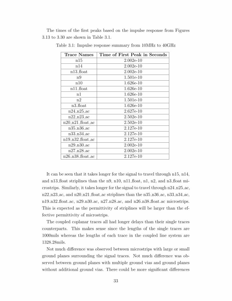
The times of the first peaks based on the impulse response from Figures
3.13 to 3.30 are shown in Table 3.1.
Table 3.1: Impulse response summary from 10MHz to 40GHz
Trace Names Time of First Peak in Secondsn15 2.002e-10n14 2.002e-10
n13 float 2.002e-10n9 1.501e-10n10 1.626e-10
n11 float 1.626e-10n1 1.626e-10n2 1.501e-10
n3 float 1.626e-10n24 n25 ac 2.627e-10n22 n23 ac 2.502e-10
n20 n21 float ac 2.502e-10n35 n36 ac 2.127e-10n33 n34 ac 2.127e-10
n19 n32 float ac 2.127e-10n29 n30 ac 2.002e-10n27 n28 ac 2.002e-10
n26 n38 float ac 2.127e-10
It can be seen that it takes longer for the signal to travel through n15, n14,
and n13 float striplines than the n9, n10, n11 float, n1, n2, and n3 float mi-
crostrips. Similarly, it takes longer for the signal to travel through n24 n25 ac,
n22 n23 ac, and n20 n21 float ac striplines than the n35 n36 ac, n33 n34 ac,
n19 n32 float ac, n29 n30 ac, n27 n28 ac, and n26 n38 float ac microstrips.
This is expected as the permittivity of striplines will be larger than the ef-
fective permittivity of microstrips.
The coupled coplanar traces all had longer delays than their single traces
counterparts. This makes sense since the lengths of the single traces are
1000mils whereas the lengths of each trace in the coupled line system are
1328.28mils.
Not much difference was observed between microstrips with large or small
ground planes surrounding the signal traces. Not much difference was ob-
served between ground planes with multiple ground vias and ground planes
without additional ground vias. There could be more significant differences
33

if the traces of the DUTs were longer or if S-parameter measurements at
higher frequencies were available.
34

CHAPTER 4
CHECKING FOR CAUSALITY
4.1 Background
All physical linear time-invariant systems must obey causality, which states
that an effect must never precede the cause. The constraint on the impulse
response of the system is given mathematically as
h(t) = 0, ∀t < 0 (4.1)
Any function can always be decomposed into even and odd components such
as
h(t) = he(t) + ho(t) (4.2)
which means that
he(t) =1
2[h(t) + h(−t)] (4.3)
ho(t) =1
2[h(t)− h(−t)] (4.4)
If equation 4.1 is true, then the odd component must be related to the even
component with the following
ho(t) =
he(t), t > 0
−he(t), t < 0(4.5)
or simply as
ho(t) = sgn(t)he(t) (4.6)
35

To look at the relationship in the frequency domain, we take the Fourier
transform on both sides to get
H(f) = He(f) +1
jπf∗He(f) (4.7)
or simply as
H(f) = He(f)− jHe(f) (4.8)
since we know that Hilbert transform of a function x is given as
x(f) = x(f) ∗ 1
πf=
1
π
∫ ∞−∞
x(f ′)
f − f ′df ′ (4.9)
Equation 4.8 shows that knowing the real part of a particular set of data
in the frequency domain enforces what the corresponding imaginary values
should be and vice versa. Otherwise causality would be violated [10].
Major obstacles in computing the Hilbert transform comes from the in-
tegration from −∞ to ∞ in equation 4.9. This is because only discrete
measured or simulated data are available, which means there will be trun-
cation and discretization errors [4]. Data points ranging from DC to infinite
frequency along with infinitesimal step sizes would be required, which is just
not possible.
4.2 Discrete Hilbert Transform
A Hilbert transform procedure for discrete data is given as
DHT{f(nT )} = f(kT ) =
2π
∑n odd
f(nT )k−n k even
2π
∑n even
f(nT )k−n k odd
(4.10)
where n is the nth sample of the original data and k is the kth sample of the
reconstructed data [5].
The proposed formulation states that treating the impulse response of
the DUT to be time-limited would be an appropriate assumption. What it
suggests next is that as long as the frequency step size is small enough, which
implies a large enough time T0 to describe the impulse response of the system,
then the reconstructed data would be accurate with small discretization error.
36

Keep in mind that uniform frequency samples are necessary for this causality
check procedure.
4.3 Sampling Theorem
The Nyquist-Shannon sampling theorem states that the sampling frequency
fs must satisfy
fs > 2B (4.11)
in order to reconstruct the time domain signal with bandwidth B. When
making S-parameter measurements with network analyzers, the frequency
response of the DUT is being sampled by evenly spaced frequency points.
Looking at the dual of equation 4.11, a similar understanding may be applied.
The sampling time needs to be at least twice as long as the slowest impulse
in the time domain, which implies that the frequency step size would need
to be at least half as small as the fundamental frequency in the frequency
domain. This is to ensure the respective peaks in the impulse response of
the DUT will be captured.
4.4 Results
The following results are generated with the dht check.m script in MATLAB
along with the S-parameter measurements of the microstrips and striplines.
The dht check.m script will use mhdrload.m to help import in the .s2p files.
The discrete Hilbert transform operation is taken care of with a custom-made
dht function.
The root mean square error (RMSE) is used to compare how close the
reconstructed real and imaginary parts of S-parameter data are to the mea-
sured real and imaginary parts of S-parameter data. RMSE is given as
RMSE =
√∑ni=1(x1,i − x2,i)2
n(4.12)
where x1,i and x2,i are the measured and reconstructed data at the ith fre-
quency point. Number of frequency points is denoted by n.
Shown in Figures 4.1 to 4.5 are the results of increasing frequency step
37

0 0.5 1 1.5 2 2.5 3 3.5 4
x 1010
−2
−1
0
1startfreq=10MHz stopfreq=40GHz numberofpoints=801 df=49987500 rms=0.063134
frequency
real(s21)uhat21
0 0.5 1 1.5 2 2.5 3 3.5 4
x 1010
−1
0
1
2startfreq=10MHz stopfreq=40GHz numberofpoints=801 df=49987500 rms=0.062399
frequency
imag(s21)vhat21
Figure 4.1: Real and imaginary S21 values through measurement andreconstruction for n9
0 0.5 1 1.5 2 2.5 3 3.5 4
x 1010
−2
−1
0
1startfreq=10MHz stopfreq=40GHz numberofpoints=51 df=799800000 rms=0.082996
frequency
real(s21)uhat21
0 0.5 1 1.5 2 2.5 3 3.5 4
x 1010
−1
−0.5
0
0.5
1startfreq=10MHz stopfreq=40GHz numberofpoints=51 df=799800000 rms=0.045833
frequency
imag(s21)vhat21
Figure 4.2: Real and imaginary S21 values through measurement andreconstruction for n9
38
0 0.5 1 1.5 2 2.5 3 3.5 4
x 1010
−1
−0.5
0
0.5
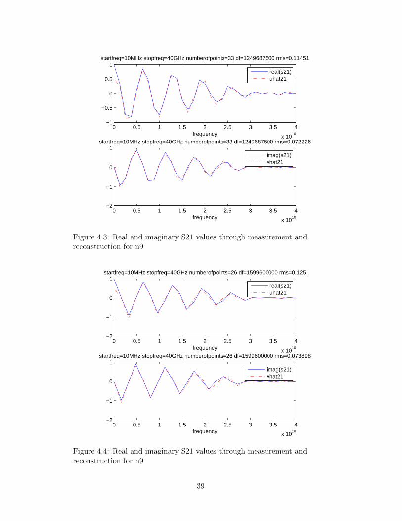
1startfreq=10MHz stopfreq=40GHz numberofpoints=33 df=1249687500 rms=0.11451
frequency
real(s21)uhat21
0 0.5 1 1.5 2 2.5 3 3.5 4
x 1010
−2
−1
0
1startfreq=10MHz stopfreq=40GHz numberofpoints=33 df=1249687500 rms=0.072226
frequency
imag(s21)vhat21
Figure 4.3: Real and imaginary S21 values through measurement andreconstruction for n9
0 0.5 1 1.5 2 2.5 3 3.5 4
x 1010
−2
−1
0
1startfreq=10MHz stopfreq=40GHz numberofpoints=26 df=1599600000 rms=0.125
frequency
real(s21)uhat21
0 0.5 1 1.5 2 2.5 3 3.5 4
x 1010
−2
−1
0
1startfreq=10MHz stopfreq=40GHz numberofpoints=26 df=1599600000 rms=0.073898
frequency
imag(s21)vhat21
Figure 4.4: Real and imaginary S21 values through measurement andreconstruction for n9
39

0 0.5 1 1.5 2 2.5 3 3.5 4
x 1010
−1
−0.5
0
0.5
1startfreq=10MHz stopfreq=40GHz numberofpoints=21 df=1999500000 rms=0.14384
frequency
real(s21)uhat21
0 0.5 1 1.5 2 2.5 3 3.5 4
x 1010
−2
−1
0
1startfreq=10MHz stopfreq=40GHz numberofpoints=21 df=1999500000 rms=0.08956
frequency
imag(s21)vhat21
Figure 4.5: Real and imaginary S21 values through measurement andreconstruction for n9
size, df, by taking an equally spaced subset of points from the original 801
frequency points. Less and less points are used in order to increase df. It can
be seen from the RMS error that as df gets large, the time-limit approxima-
tion of the impulse response of the DUT is gradually getting worse. Larger df
results in larger discretization error. The reconstructed data at the smallest
and largest frequencies available are not as accurate due to truncation error.
The frequency points in between seem to come in good agreement as long as
df is small enough.
The real and imaginary S21 RMS errors with respect to frequency step
size df figures are generated with the auto.m script. Figures 4.6 to 4.8 give a
closer look as to how the RMS errors are affected by df. Frequency step size
df and the time t it is equivalent to in the impulse response are related by
df =1
2t(4.13)
Labeled peaks of the impulse response in Figure 4.6 correspond to the equiv-
alent df labels in Figures 4.7 and 4.8. It can be seen that RMS error gets
worse as more and more peaks in the impulse response get neglected due to
40

0 1 2 3 4 5 6
x 10−10
0
0.05
0.1
0.15
0.2
0.25
0.3
0.35
0.4 X: 1.501e−10Y: 0.4227
n9(10MHz).s2p impulse response derived from ifft of s21
time in seconds
mag
nitu
de
X: 2.627e−10Y: 0.01559
X: 2.002e−10Y: 0.02633
X: 4.629e−10Y: 0.02374
Figure 4.6: n9 with start freq = 10MHz and stop freq = 40GHz and labeledpeaks
0 1 2 3 4 5
x 109
0
0.1
0.2
0.3
0.4
0.5
0.6
0.7
0.8
0.9
X: 3.349e+09Y: 0.635
real s21 rms error vs frequency step size df
frequency step size df
rms
erro
r
X: 2.499e+09Y: 0.1683
X: 1.9e+09Y: 0.1364X: 1.1e+09
Y: 0.1001
Figure 4.7: Real S21 RMS error vs frequency step size df for n9 withcorresponding labels
41

0 1 2 3 4 5
x 109
0
0.1
0.2
0.3
0.4
0.5
0.6
0.7
0.8
0.9
X: 1.1e+09Y: 0.06438
imag s21 rms error vs frequency step size df
frequency step size df
rms
erro
r
X: 1.9e+09Y: 0.0755
X: 2.499e+09Y: 0.09326
X: 3.349e+09Y: 0.4989
Figure 4.8: Imaginary S21 RMS error vs frequency step size df for n9 withcorresponding labels
larger df. RMS error makes a big jump at df=3.349GHz when a large peak
at 0.1501ns has been neglected.
42

Additional examples are shown in Figures 4.9 to 4.14. This is to verify
that the same observation was made with S parameters of coupled lines.
0 2 4 6 8 10 12 14 16 18
x 10−10
0
0.005
0.01
0.015
0.02
0.025
0.03
0.035
X: 1.276e−09Y: 0.004519
n22_n23_ab(10MHz).s2p impulse response derived from ifft of s21
time in seconds
mag
nitu
de
X: 9.258e−10Y: 0.008248
X: 6.381e−10Y: 0.021
Figure 4.9: n22 & n23 AB with start freq = 10MHz and stop freq = 40GHzand labeled peaks
43

0 1 2 3 4 5
x 109
0
0.02
0.04
0.06
0.08
0.1
0.12
X: 7.998e+08Y: 0.05586
real s21 rms error vs frequency step size df
frequency step size df
rms
erro
r
X: 5.499e+08Y: 0.02987
X: 3.499e+08Y: 0.009412
Figure 4.10: Real S21 RMS error vs frequency step size df for n22 n23 abwith corresponding labels
0 1 2 3 4 5
x 109
0
0.02
0.04
0.06
0.08
0.1
0.12
X: 3.499e+08Y: 0.009862
imag s21 rms error vs frequency step size df
frequency step size df
rms
erro
r
X: 5.499e+08Y: 0.03064
X: 7.998e+08Y: 0.05468
Figure 4.11: Imaginary S21 RMS error vs frequency step size df for n22 n23ab with corresponding labels
44

0 0.5 1 1.5 2
x 10−9
0
0.005
0.01
0.015
0.02
0.025
0.03
0.035
X: 6.756e−10Y: 0.02351
n22_n23_ad(10MHz).s2p impulse response derived from ifft of s21
time in seconds
mag
nitu
de
X: 1.126e−09Y: 0.004324
Figure 4.12: n22 & n23 AD with start freq = 10MHz and stop freq =40GHz and labeled peaks
0 1 2 3 4 5
x 109
0
0.02
0.04
0.06
0.08
0.1
0.12
0.14
0.16
X: 7.498e+08Y: 0.06094
real s21 rms error vs frequency step size df
frequency step size df
rms
erro
r
X: 4.499e+08Y: 0.01303
Figure 4.13: Real S21 RMS error vs frequency step size df for n22 n23 adwith corresponding labels
45

0 1 2 3 4 5
x 109
0
0.02
0.04
0.06
0.08
0.1
0.12
0.14
0.16
X: 7.498e+08Y: 0.05838
imag s21 rms error vs frequency step size df
frequency step size df
rms
erro
r
X: 4.499e+08Y: 0.01313
Figure 4.14: Imaginary S21 RMS error vs frequency step size df for n22 n23ad with corresponding labels
46

Shown in Figures 4.15 and 4.16 are the complete RMS error vs frequency
step size df plots sweeping from the smallest df to the largest df possible given
the 801 frequency points from measured data. The smallest df would have
801 points whereas the largest df would have two points spaced at 10MHz
and 40GHz. It can be seen that past a certain df, the RMS error oscillates
back and forth depending on where the small number of sampled frequency
points are. Certain frequency spacings may coincidentally work very well or
very poorly at this stage since there are so few points left. Not much may
be revealed as to whether the small number of S-parameter data are causal
or not.
0 0.5 1 1.5 2 2.5 3 3.5 4
x 1010
0
0.1
0.2
0.3
0.4
0.5
0.6
0.7
0.8
0.9real s21 rms error vs frequency step size df
frequency step size df
rms
erro
r
Figure 4.15: Real S21 RMS error vs frequency step size df for n9
47

0 0.5 1 1.5 2 2.5 3 3.5 4
x 1010
0
0.1
0.2
0.3
0.4
0.5
0.6
0.7
0.8
0.9imag s21 rms error vs frequency step size df
frequency step size df
rms
erro
r
Figure 4.16: Imaginary S21 RMS error vs frequency step size df for n9
48

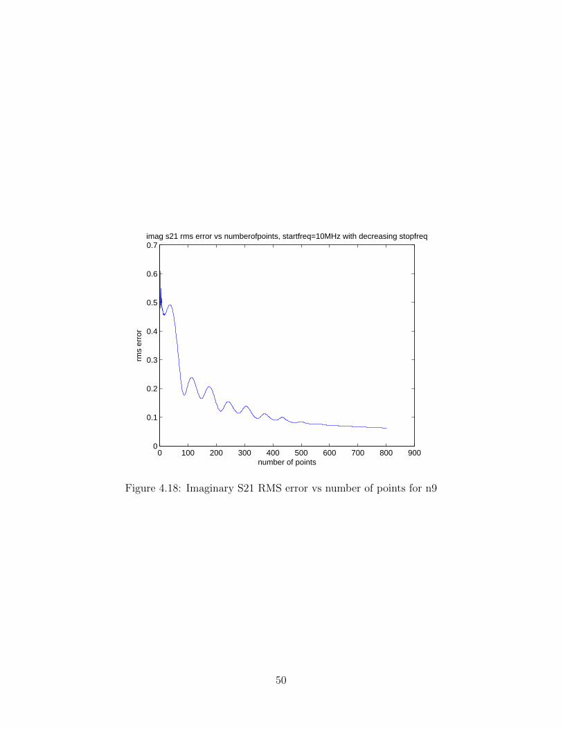
Shown in Figures 4.17 and 4.18 are the results of decreasing the stop fre-
quency while maintaining the same df and start frequency of 10MHz. Re-
moving the high-frequency data in this case made the RMS error higher.
That is because there are less sets of points now used to compute the RMS
error. The amount of contribution to the RMS error for each set of points
has increased. As a result the truncation error at the lowest and highest
remaining frequency points are made more apparent.
0 100 200 300 400 500 600 700 800 9000
0.1
0.2
0.3
0.4
0.5
0.6
0.7
0.8
0.9
1real s21 rms error vs numberofpoints, startfreq=10MHz with decreasing stopfreq
number of points
rms
erro
r
Figure 4.17: Real S21 RMS error vs number of points for n9
49
0 100 200 300 400 500 600 700 800 9000
0.1
0.2
0.3
0.4
0.5
0.6
0.7imag s21 rms error vs numberofpoints, startfreq=10MHz with decreasing stopfreq
number of points
rms
erro
r
Figure 4.18: Imaginary S21 RMS error vs number of points for n9
50

Shown in Figures 4.19 and 4.20 are the results of increasing the start fre-
quency while maintaining the same df and stop frequency of 40GHz. Having
less points does not necessarily mean the RMS error would rise. In this case
the magnitude of the S parameters from the remaining frequency points are
a lot smaller than the ones that have been cut out. So RMS error actually
decreased with removing the low-frequency data.
0 100 200 300 400 500 600 700 800 9000
0.01
0.02
0.03
0.04
0.05
0.06
0.07
0.08
0.09real s21 rms error vs numberofpoints, stopfreq=40GHz with increasing startfreq
number of points
rms
erro
r
Figure 4.19: Real S21 RMS error vs number of points for n9
51

0 100 200 300 400 500 600 700 800 9000
0.01
0.02
0.03
0.04
0.05
0.06
0.07
0.08
0.09imag s21 rms error vs numberofpoints, stopfreq=40GHz with increasing startfreq
number of points
rms
erro
r
Figure 4.20: Imaginary S21 RMS error vs number of points for n9
52

Shown in Figure 4.21 is the reconstructed S11 parameter of n9 with a start
frequency of 10MHz and a stop frequency of 40GHz with a total of 801 evenly
spaced frequency points. The discrete Hilbert transform seems capable of
tracing the overall shape of the measured S11 data, but there seems to be
a difference in offset looking at the real part, and a difference in orientation
when looking at the imaginary part. Shown in Figure 4.22 are reconstructed
S11 parameter of n9 with a start frequency of 300kHz and a stop frequency
of 9GHz with a total of 801 evenly spaced frequency points. The difference
in offset when looking at the real part, and the difference in orientation when
looking at the imaginary part, are still present when comparing Figures 4.21
and 4.22. Similar 2-port S11 reconstruction problems were observed when
using other sets of measured data. The reason could be the general shape of
the data. The measured 2-port S11 data could be not square-integrable.
0 0.5 1 1.5 2 2.5 3 3.5 4
x 1010
−1
−0.5
0
0.5startfreq=10MHz stopfreq=40GHz numberofpoints=801 df=49987500 rms=0.40089
frequency
real(s11)uhat11
0 0.5 1 1.5 2 2.5 3 3.5 4
x 1010
−1
0
1
2startfreq=10MHz stopfreq=40GHz numberofpoints=801 df=49987500 rms=0.27028
frequency
imag(s11)vhat11
Figure 4.21: 2-port S11 measurement of n9 with start freq = 10MHz andstop freq = 40GHz
53

0 1 2 3 4 5 6 7 8 9
x 109
−0.6
−0.4
−0.2
0
0.2startfreq=300kHz stopfreq=9GHz numberofpoints=801 df=11249625 rms=0.097219
frequency
real(s11)uhat11
0 1 2 3 4 5 6 7 8 9
x 109
−0.4
−0.2
0
0.2
0.4startfreq=300kHz stopfreq=9GHz numberofpoints=801 df=11249625 rms=0.13247
frequency
imag(s11)vhat11
Figure 4.22: 2-port S11 measurement of n9 with start freq = 300kHz andstop freq = 9GHz
54

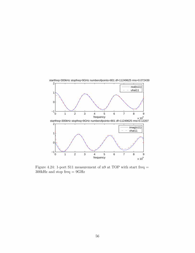
Shown in Figure 4.23 is the reconstructed 1-port S11 parameter of n9 with
a start frequency of 10MHz and a stop frequency of 40GHz with a total
of 801 evenly spaced frequency points. Larger discrepancies are observed
throughout the real part of S11 and the higher frequency data points of the
imaginary part of S11. Shown in Figure 4.24 is the reconstructed 1-port S11
parameter of n9 with a start frequency of 300kHz and a stop frequency of
9GHz with a total of 801 evenly spaced frequency points. A better match was
found when higher frequency data was thrown out in this case as shown in
Figure 4.24. It seems that the higher frequency data from this measurement
are not as well-behaved for the discrete Hilbert transform operation. Similar
1-port S11 reconstruction problems were observed when using other sets of
measured data. The reason could be the general shape of the data. The
measured 1-port S11 data could be not square-integrable with the higher
frequency data present.
0 0.5 1 1.5 2 2.5 3 3.5 4
x 1010
−1
0
1
2startfreq=10MHz stopfreq=40GHz numberofpoints=801 df=49987500 rms=0.38526
frequency
real(s11)uhat11
0 0.5 1 1.5 2 2.5 3 3.5 4
x 1010
−2
−1
0
1
2startfreq=10MHz stopfreq=40GHz numberofpoints=801 df=49987500 rms=0.27517
frequency
imag(s11)vhat11
Figure 4.23: 1-port S11 measurement of n9 at TOP with start freq =10MHz and stop freq = 40GHz
55
0 1 2 3 4 5 6 7 8 9
x 109
−1
0
1
2startfreq=300kHz stopfreq=9GHz numberofpoints=801 df=11249625 rms=0.072439
frequency
real(s11)uhat11
0 1 2 3 4 5 6 7 8 9
x 109
−1
0
1
2startfreq=300kHz stopfreq=9GHz numberofpoints=801 df=11249625 rms=0.12207
frequency
imag(s11)vhat11
Figure 4.24: 1-port S11 measurement of n9 at TOP with start freq =300kHz and stop freq = 9GHz
56

One limitation of the discrete Hilbert transform is that the data must be
square-integrable [11]. Figure 4.25 shows an example. The hypothetical data,
s21, is a constant one across 801 evenly spaced frequency points, which is not
a square-integrable function. The causal reconstruction of such a frequency
response according to the discrete Hilbert transform is given as -dht(s21).
However, when trying to derive the real part of s21 based on -dht(s21), we
get dht(-dht(s21)). It is clear that the proposed dht(-dht(s21)) does not
match up with the original s21 hypothetical data.
0 100 200 300 400 500 600 700 800 900−3
−2
−1
0
1
2
3
equally spaced frequency points
reconstructing real part of s21 with derived imaginary part of s21
s21−dht(s21)dht(−dht(s21))
Figure 4.25: Example where the discrete Hilbert transform fails
57

CHAPTER 5
CONCLUSIONS
Measuring the S parameters of the microstrips and striplines was successful.
The board file was very descriptive of the physical properties of the DUTs.
A greater in-depth look at the dimensions may be done by reading from the
.brd file directly if needed. The S parameters made sense as the time delay
of the impulse response between the different DUTs matched up with the
physical properties. The amplitude of the S21 parameters started to decay
past 25GHz or so, which is expected due to loss from the FR-4 substrate
along with the physical limitations associated with 3.5mm cables trying to
support pure TEM mode signals.
Reconstructing S21 data from different ranges of frequencies using the
discrete Hilbert transform matched well with the original measured S21 data.
The discrete Hilbert transform was able to reconstruct S21 measurements
with small errors by using only high-frequency data even with low-frequency
data being neglected. It seems that the discrete Hilbert transform can provide
accurate results as long as the range of sampled S-parameter data is square-
integrable, and there are sufficient numbers of points with a small enough,
equally spaced frequency step size df to capture the response of the DUT.
It may be worth investigating why using the discrete Hilbert transform to
reconstruct S11, S22 of 2-port measurements and S11 of 1-port measurements
was a lot less accurate than using S21, S12 of 2-port measurements. It may
have to do with the frequency response for S11, S22 of 2-port measurements
and S11 of 1-port measurements not being square-integrable.
58
REFERENCES
[1] P. Triverio, S. Grivet-Talocia, M. S. Nakhla, F. G. Canavero, andR. Achar, “Stability, Causality, and Passivity in Electrical InterconnectModels,” IEEE Transactions on Advanced Packaging, vol. 30, no. 4, pp.795–808, Nov. 2007.
[2] S. Asgari, S. N. Lalgudi, and M. Tsuk, “Analytical Integration-basedCausality Checking of Tabulated S-parameters,” in Electrical Perfor-mance of Electronic Packaging and Systems, Austin, TX, USA, Oct.2010, pp. 189–192.
[3] B. Young and A. S. Bhandal, “Causality Checking and Enhancementof 3D Electromagnetic Simulation Data,” in Electrical Performance ofElectronic Packaging and Systems, Austin, TX, USA, Oct. 2010, pp.81–84.
[4] P. Triverio and S. Grivet-Talocia, “Robust Causality Characterizationvia Generalized Dispersion Relations,” IEEE Transactions on AdvancedPackaging, vol. 31, no. 3, pp. 579–593, Aug. 2008.
[5] S. C. Kak, “The Discrete Hilbert Transform,” Proceedings of the IEEE,vol. 58, pp. 585–586, Apr. 1970.
[6] “Cadence Allegro Downloads,” 2012. [Online]. Available:http://www.cadence.com/products/pcb/Pages/downloads.aspx
[7] “Cascade Microtech Fixed Pitch Compliant Probe,” 2012. [On-line]. Available: http://www.cmicro.com/products/probes/signal-integrity/fpc-probe/fixed-pitch-compliant-probe
[8] “Picoprobe by GGB Industries Calibration Substrates,” 2012. [Online].Available: http://www.ggb.com/calsel.html
[9] “MATLAB Central File Exchange mhdrload.m,” 2012. [Online]. Avail-able: http://www.mathworks.com/matlabcentral/fileexchange/2973
[10] S. H. Hall and H. L. Heck, Advanced Signal Integrity for High-SpeedDigital Designs. Hoboken, NJ: John Wiley & Sons, Inc., 2009.
59

[11] H. M. Nussenzveig, Causality and Dispersion Relations. New York,NY: Academic Press, Inc., 1972.
60
Recommended