Download pdf - Calibrating regulatory minimum capital requirements … · Working group members ... Calibrating regulatory minimum capital requirements ... to conduct a “top-down” assessment

Basel Committee on Banking Supervision

Calibrating regulatory minimum capital requirements and capital buffers: a top-down approach

October 2010

Copies of publications are available from:

Bank for International Settlements Communications CH-4002 Basel, Switzerland

E-mail: [email protected]

Fax: +41 61 280 9100 and +41 61 280 8100

This publication is available on the BIS website (www.bis.org).

© Bank for International Settlements 2010. All rights reserved. Brief excerpts may be reproduced or translated provided the source is cited.

ISBN 92-9131-852-3 (print)

ISBN 92-9197-852-3 (online)


Contents

I. Overview and executive summary ..................................................................................1 I.A. Conceptual framework ...........................................................................................1 I.B. Regulatory minimum requirements ........................................................................2 I.C. Capital buffers ........................................................................................................3 I.D. Leverage ratio ........................................................................................................4 I.E. Risk-weighted assets .............................................................................................4 I.F. Caveats ..................................................................................................................4 I.G. Summary of calibration findings .............................................................................5

II. Detailed discussion of the findings ..................................................................................6 II.A. Regulatory minimum requirements ........................................................................6 II.B. Buffers....................................................................................................................9 II.C. Leverage ratio ......................................................................................................16

Working group members ........................................................................................................19

Calibrating regulatory minimum capital requirements and capital buffers: a top-down approach 1


I. Overview and executive summary

As part of its work to strengthen global capital requirements, the Basel Committee on Banking Supervision established a working group to conduct a “top-down” assessment of the overall level of capital requirements that should be held within the banking system. The working group was tasked with undertaking empirical analysis to inform the calibration of the common equity and Tier 1 risk-based ratios and the Tier 1 leverage ratio, as well as the regulatory buffers above the common equity and Tier 1 risk-based ratios. This analysis represented one of the inputs to the Committee’s calibration of the new capital framework, and complements the cost-benefit analysis conducted by the Long-Term Economic Impact (LEI) group and the detailed “bottom up” Quantitative Impact Study (QIS) of the effects of the proposed regulatory reforms on individual banks.

This note summarises the findings of the top-down calibration work. In particular, it provides a conceptual framework for the calibration work, describes the various empirical exercises that were performed, and summarises the results.

It is important to highlight that there is not a single correct approach to determine the calibration, nor is there a single model that can be used to provide the “right” answer. The approach adopted in this paper, therefore, is to generate information from a range of sources and from a variety of perspectives. In the face of uncertainty, the combination of many estimates will produce better outcomes than reliance on a single estimate or approach. Also, as explained in the paper, a number of caveats need to be carefully kept in mind when interpreting the results, primarily relating to the use of historical data generated under a regulatory regime different from that which will prevail in the future.

I.A. Conceptual framework An appropriate starting point for calibration is to first establish a conceptual framework outlining the role of minimum capital and buffer requirements, along with strategies and methods for putting these concepts into practice. The following high-level concepts are adopted in this paper: the regulatory minimum requirement is the amount of capital needed for a bank to be regarded as a viable going concern by creditors and counterparties, while a buffer can be seen as an amount sufficient for the bank to withstand a significant downturn period and still remain above minimum regulatory levels.1 An overview of the strategies and empirical work undertaken to inform the high-level concepts is provided in the remainder of this section. Further details are contained in the third section of the paper, which also presents the results.

1 The definition of the buffer draws directly from the December 2009 Consultative Document, which stated that

the capital conservation buffer “...should be capable of being drawn down through losses and large enough to enable banks to maintain capital levels above the minimum requirement throughout a significant sector-wide downturn.” (Basel Committee on Banking Supervision, “Strengthening the Resilience of the Banking Sector”, December 2009)

2 Calibrating regulatory minimum capital requirements and capital buffers: a top-down approach

I.B. Regulatory minimum requirements It is not possible to directly observe the minimum amount of capital needed for a bank to be viewed as viable and solvent by investors and creditors, including short-term funding providers. Presumably, market participants make some assessment of the likelihood and size of shocks that they expect a bank to be able to withstand, and transact only with those banks that they believe have a high probability of remaining solvent in the future, consistent with their risk tolerance. Unfortunately, we cannot observe these market assessments directly. Further, the assessments will vary across institutions and over time given differences in business models and as macroeconomic and banking industry environments change. An additional complication is that the level of capital demanded by market participants may be influenced by historical regulatory requirements and the perceived costs of falling below those ratios. This introduces a certain circularity into the relationship between historical ratios, regulatory ratios and assessments of potential losses.

In the face of these factors, one operational approach is to examine the distribution of historical earnings in the banking industry under the assumption that a high percentile net loss realisation for a typical bank is a good approximation of the market’s ex ante, unconditional view of going-concern capital sufficiency. This seems an appropriate benchmark for a risk-based regulatory capital standard that applies across all banks for all points in time. In this regard, it is important to note that risk-weighted assets are intended to capture differences in risk across institutions, so that the task in calibrating a minimum regulatory requirement is to find a minimum amount of capital relative to each firm’s risk that seems consistent with a bank being viewed as a viable going concern.

To put this approach into practice, analysis of the “Return on Risk-Weighted Assets” (RORWA) was undertaken, using data on net income for a large set of banking companies in seven member countries over relatively long time periods.2 Each country looked at the ratio of net income to risk-weighted assets (RWA) for each bank in every period that company was in the sample, and then examined the left-hand (negative net income) “tail” of the distribution. High percentiles of this distribution might be a reasonable proxy value for the degree of “shock” that market participants would expect banks to be able to withstand.

The RORWA analysis focused on the volatility of realised net income as a measure of potential loss and capital needs for a bank. Since negative net income feeds directly to common equity via declines in retained earnings, it has comparable effects on both Tier 1 and the common equity component of Tier 1 (holding other deductions constant). One question, therefore, is whether the analysis of net income is most directly applicable to calibration of the Tier 1 capital or common equity-risk based ratio.

There are reasonable arguments on both sides. One argument is that losses via negative net income feed directly into common equity, and thus the RORWA analysis is most relevant for calibration of the regulatory minimum level of the common equity risk-based ratio. An alternative view is that other Tier 1 capital components are also loss-absorbing and can protect creditors, and thus the RORWA work is best applied to the Tier 1 ratio. To some extent, the balance of the argument depends on the extent to which the non-common elements of Tier 1 capital are viewed as contributing to a banking company’s viability. The experience of the recent crisis suggests that in many cases market participants viewed the

2 This approach is derived from Andrew Kuritzkes and Til Schuermann, “What We Know, Don’t Know and Can’t

Know about Bank Risk: A View from the Trenches.” In The Known, the Unknown and the Unknowable in Financial Risk Management, ed. F.X. Diebold, N. Doherty, and R.J. Herring. Princeton University Press. (March 2008).


non-common components of Tier 1 as less useful as a loss absorber or less relevant as a determinant of viability in periods of acute stress. This implies that a reasonable baseline for the RORWA analysis around potential stressed losses would be the amount of common equity needed for the minimum regulatory requirement, and this is the approach followed in this analysis.3

I.C. Capital buffers To help determine the size of a buffer large enough for a bank to withstand a significant downturn period and remain above regulatory minimum capital levels, analysis of actual historical experience and the results of recent stress tests, both singly and in combination, was undertaken. Both realised loss experience during the current and past crises and projections of losses (negative net income or impact on Tier 1 capital or common equity) made during the recent crisis are relevant metrics for assessing the possible impact of severe stress and thus for sizing the capital buffer.

• Current and Historical Crisis Losses – this examines cumulative losses (negative net income, as a proxy for the impact on Tier 1 capital and the common equity component of Tier 1 capital) that banking companies sustained during the recent global financial crisis and peak losses during past financial crises in individual jurisdictions or regions.

• Stress tests – the projected decreases in capital from stress tests conducted by eight member countries during the recent financial crisis are examined. In addition, results for individual banking companies for one country are also examined, to provide a sense of the dispersion underlying aggregate or average countrywide numbers. An important challenge in interpreting the results of this work is to address the lack of comparability in the stress tests conducted by different countries.

• The RORWA analysis was also used to help calibrate the supervisory buffer, as that analysis provides information about large, negative shocks to income and capital.

These exercises reveal considerable diversity across banks in the size of current and past crisis-related losses. In thinking about calibration, one important question is how to interpret this diversity of experience. Should the buffer be set relative to the average or typical experience across banks (that is, as the weighted average or median) or should the buffer be set as a higher percentile of the cross-sectional experience (for instance, the 75th percentile outcome, the 95th percentile outcome, or the maximum)? In general, all available information is considered, so that calibration of the buffers could be determined in light of the full range of experience across banks and countries, acknowledging that the analysis does not identify the sources of historical losses that may differentiate between business models and the source and incidence of the next banking crisis cannot be known.

3 As an additional benchmark, a range of regulatory and other capital ratios from the period immediately before

and in the early phases of the financial crisis were examined. The idea was to see if there was a “critical value” of each ratio such that banks that eventually became severely stressed during the crisis tended to have capital ratios below this level, while less stressed banks tended to have ratios above it. The analysis, which is described in greater detail in the discussion of the leverage ratio, was used as a supplement to the analysis based on historical earnings, primarily as a means of benchmarking the results of the RORWA analysis against recent historical experience. This type of analysis, almost by definition, will imply critical values greater than the regulatory minimum stipulated in the pre-crisis regulation given that the minimum is typically the point of resolution and funding markets are likely too close to an institution before it reaches this point. In addition, the results are highly sensitive to the critical value limit used. This may reduce the reliability of using these critical values as a guide to the optimal level of the minimum capital requirement.


I.D. Leverage ratio The calibration of a backstop Tier 1 leverage ratio is not addressed in the same way as the risk-based ratios. The longer testing and transition period associated with the leverage ratio as compared to the new risk-based ratio standards is intended to provide a period to examine the performance and calibration of the leverage ratio in “parallel run” mode. That said, information was collected on historical trends in leverage in the banking systems of ten member countries. This data includes information on trends in traditional leverage – capital relative to balance sheet assets – as well as information on trends in different elements of Tier 1 capital, in risk-weighted to total assets and in the impact of off-balance sheet positions on overall leverage. As noted, these measures provide a sense of recent historical trends that is useful background for calibration, but do not lead directly to suggested regulatory requirements.

An analysis was also undertaken of the differences in leverage ratios between banks that eventually became severely stressed during the crisis and less stressed banks. The pre-crisis and early crisis leverage ratios were defined as Tier 1 capital to total assets, common equity to total assets, common equity minus Tier 1 deductions to total assets, or tangible common equity to tangible assets. This analysis provides a very general sense of the levels of these ratios that discriminated between severely stressed and other banks prior to the crisis, and thus provides valuable context to the possible calibration of a new leverage ratio.

I.E. Risk-weighted assets Much of the calibration work described above uses historical levels of risk-weighted assets as the denominator – that is, most of the analysis scales results by risk-weighted assets, but by necessity, the risk-weighted assets use historical values, either on a Basel I or Basel II basis. Of course, the Basel Committee reforms will result in significant changes to the level of risk-weighted assets that would apply to a given activity or set of positions.

I.F. Caveats As noted, there are some significant caveats that must be considered in weighing the results of the work presented in this report. Much of the work relies on analysis of historical data, either from the recent crisis or from past crises. The benefit of using such data is that they reflect actual realised outcomes for large banks across multiple jurisdictions, thus grounding the work in real history and events. The shortcoming of using cross country historical data is that they are not perfectly consistent across jurisdictions. It is not possible, for example, to isolate the impact of Basel II versus Basel I in the computations, or differences in the definition of capital. Moreover, the historical data reflect outcomes under different regulatory capital regimes than will prevail under the revised Basel standards. This means that the data reflect regulatory restrictions, a range of banking sector and macroeconomic environments, and bank behaviour that will almost certainly differ from those prevailing in the future. The losses that banks would have experienced had the new, more risk-sensitive Basel capital and liquidity requirements been in place might have been smaller than the losses actually sustained. In addition, improvements in the quality of the capital base should make banks more resilient to shocks in the future.

Conversely, data from the recent and previous financial crises are also affected by official sector actions – capital injections, liquidity facilities, liability guarantees – that may have significantly altered realised losses and revenues, probably improving them relative to what they would have been in the absence of official intervention. In addition, the analysis conducted in this report is subject to survivorship bias, as losses from banks that failed are not always fully captured in the analyses. This biases down the estimates. Further, some


numbers exclude mark-to-market variation of “available for sale” assets that is not included in accounting income (but which is deducted directly from capital). More generally, most of the analysis focuses on losses incurred by banks and does not reflect how much additional capital would have been needed to maintain a reasonable level of lending during the crisis to help avert adverse “credit crunch” effects. In gauging the results, these caveats need to be kept firmly in mind.

I.G. Summary of calibration findings The table below provides a high-level summary of the calibration results for the regulatory minimum capital requirement for the common equity-based ratio and for the buffer above that ratio, and some indicative findings for the leverage ratio. These are all based on historical definitions of risk-weighted assets (in the case of the minimum requirement and the buffer) and of Tier 1 capital and Tier 1 deductions (in the case of the leverage ratio findings). The table reports the mean and median results across countries of the various empirical exercises, as well as minimum and maximum values, to provide a sense of the range of results. In many cases, the country-level results are themselves averages of individual bank data, so there is further diversity of findings not captured in the table. This diversity of experience seems particularly important to recall when considering average results for calibration purposes, which is geared towards identifying the tails of loss distributions. More detailed explanations and discussion of the findings, importantly including discussion of caveats of the analysis, are contained in the remainder of this paper.

In determining the level of the new prudential requirements, judgements need to be made about the appropriate benchmarks for the severity of crises and the performance of individual banks during different crises. At one extreme, there are the largest losses experienced by banks during the most severe crises, while at another extreme one could consider average bank losses experienced during more frequent but less severe crises. This report does not in and of itself provide an answer as to the right choice, and should be read as informing, and not prejudging, such judgements.


High-level summary table: Range of calibration results

Minimum Max. Arithmetic Mean Median Countries

#

Calibration of the minimum

RORWA (large bank results) 99th percentilea +0.89% -8.66% -3% -4% 7 99th percentile, excluding gainsa -0.18% -8.66% -4% -5% 6 Maximuma +0.89% -41.5% -10% -5% 6 Maximum, excluding outliers and gainsa -2.71% -6.83% -5% -5% 5

Calibration of the regulatory buffers

Historical lossesd Peak losses / RWA 0.00% -29.2% -3% -1.0% 7b Peak losses / RWA – systemic crises -0.09% -29.2% -7% -3.7% 4b

Losses during the recent crisisd Pre-tax net income / RWA -0.60% -25.7% -5% -3% 14 Stress testsd Tier 1 capital / RWA -1.2% -4.0% -3% -3% 6c

Calibration of the leverage ratio

Critical valuese Range

Tier 1 Capital / Assets 3.0% - 5.0% 19 Common Equity / Assets 3.0% - 4.0% 19 Tangible Common Equity / Tangible Assets 2.5% - 4.0% 19 Common Equity minus Tier 1 Deductions / Assets 2.5% - 4.5% 19

a. The 99th percentile or maximum is first determined within each country. The data presented in each row summarises the data across countries. Because of insufficient data, percentiles higher than the 99th percentile cannot be identified in some countries’ samples. While 99th percentile values are reported in this table, higher percentiles may be more reasonable measures for calibration purposes.

b. This refers to the number of crisis episodes. The averages and ranges reported are based on individual bank figures.

c. Individual bank stress test results in a number of countries are significantly more severe than -4.0%.

d. Results for banks experiencing losses during the stress period. For the historical loss results, these are peak losses; for the recent crisis these are cumulative losses; for the stress tests, these are average losses for banks subject to the stress test and do not include losses already incurred prior to the stress test period.

e. Levels of the ratio at which at least 50% of banks that became severely stressed during the financial crisis and 50% of banks that did not become severely stressed.

II. Detailed discussion of the findings

II.A. Regulatory minimum requirements Seven member countries calculated “return on risk-weighted assets” (RORWA) for banks in their jurisdictions over relatively long historical periods. For each bank in each time period, RORWA is calculated as the ratio of net income to risk-weighted assets. The distribution of this ratio across all observations in each country’s data set, or for subsets of observations, is calculated.


The analysis focused on the left-hand (negative net income) “tail” of the distribution. This part of the distribution contains the largest losses relative to RWA, and thus is most relevant for capital calibration purposes – conceptually this is quite similar to a “Value-at-risk” measure. High percentiles of the income distribution might be a reasonably proxy value for the degree of “shock” that market participants would expect banks to be able to withstand. Of course, there are important differences across countries in the risk profiles of the banking sector that will affect the results produced for each country.

There are significant caveats in making comparisons in the results from different countries. To begin, some countries calculated RORWA for both pre-tax and after-tax net income, while other countries reported on just one basis or the other. Further, while most countries calculated RORWA on a one-year basis (that is, using annual net income), at least one country used semi-annual data. Finally, there are differences across countries as to whether risk-weighted assets were computed on a Basel I or Basel II basis. Some countries’ data reflects a mix of both, as banks transitioned from Basel I to Basel II over the historical period examined, at least one is entirely on a Basel I basis, and another presented data on both bases.

There are also important differences in sample size and in the length of the historical horizon used in the analysis. The historical sample period varied from 5 to 29 years (that is, the longest was from 1981 to 2009, while the shortest was from 2005 to 2009). Similarly, the number of banks included in the sample also varied, from as few as 4 to as many as 300 to 400. However, some countries whose data covered larger numbers of banks also broke out a “large bank” subsample, and these are somewhat more comparable across countries. Focusing on just the large bank subsample for those countries that provided them, in combination with the full samples for those countries whose data covered fewer banks, the number of banks included in the analysis ranges from 4 to 20.

Overall, these differences meant that the sample sizes varied significantly across countries, as did the number of business cycles included in the data. The samples generally contained between 200 and 600 observations, which means the very high tails of the distribution could not truly be identified because there were not enough observations to populate this fine a decomposition of the distribution. (For example, the 99.9th percentile of the distribution cannot be identified if there are fewer than 1000 observations in the sample.) In most cases, the countries reported these high percentiles by repeating the largest (most negative) observation in the sample.

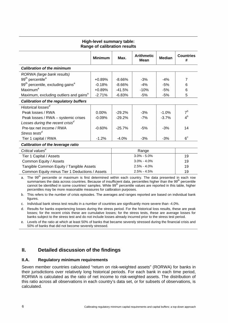
The main results are illustrated in Figures 1 and 2. The figures report results for large bank samples, for countries that provided this decomposition, and for full samples for countries that did not. In general, the negative “tails” of the net income-to-RWA distribution are smaller for larger banks than for smaller ones. These smaller tail events could reflect differences in diversification and business focus, as well as the impact of official intervention when large banks are in distress. To avoid extreme outliers in the data owing to small bank size, the working group focused on the results for large banks, where those were provided.

Turning to the rest of the results, one question is which percentile of the distribution to consider; there is certainly no single theoretically “correct” answer. At one end of the spectrum, we can consider the 99th percentile, as nearly all the samples are large enough to identify this percentile. The 99th percentile figures for large banks range between 0.89% and -8.66% (see Figure 1). The mean value across all the large bank samples is approximately -3.20% and the median is about -4.0%. Excluding the observations reflecting positive net income in the tails, the mean value is about -4.0% and the median is about -4.9%.


-10.00

-8.00

-6.00

-4.00

-2.00

0.00

2.00

1 2 3 4 5 6 7 8 9 10 11

Figure 1Return on Risk-Weighted Assets

99th Percentile Results

Bars are the 99th percentile of the distribution of net income to risk-weighted assets based on data submitted by seven member countries. Some countries submitted more than one sample, using different definitions of net income (pre-tax and after-tax) or different definitions of risk-weighted assets.

-45.00

-40.00

-35.00

-30.00

-25.00

-20.00

-15.00

-10.00

-5.00

0.00

5.00

1 2 3 4 5 6 7 8 9 10 11

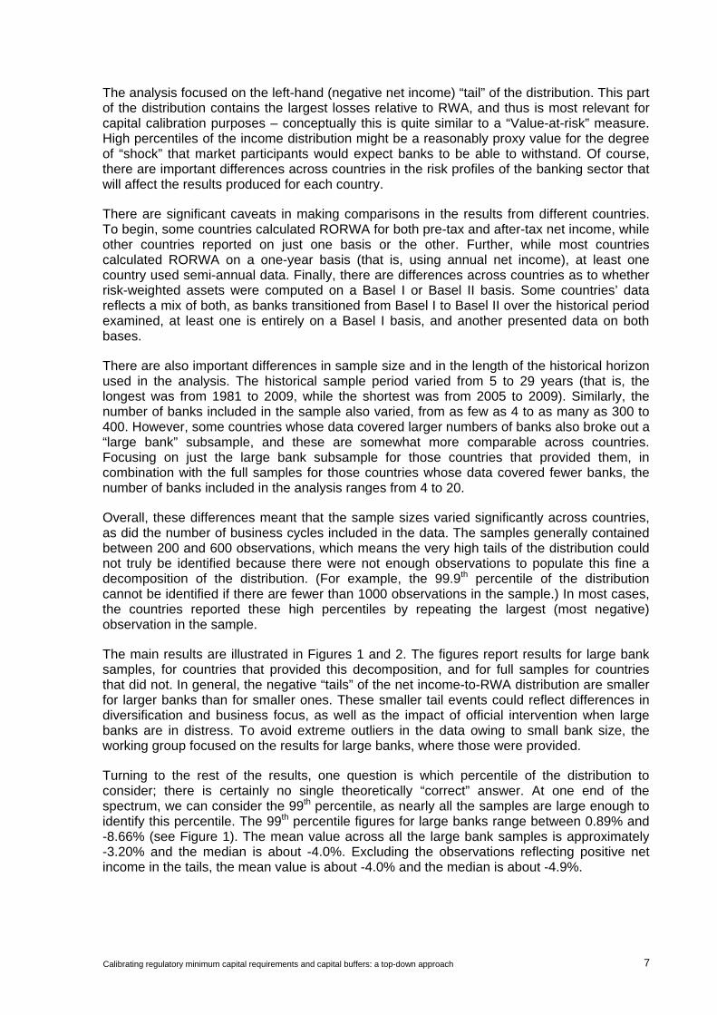
Figure 2Return on Risk-Weighted Assets

Maximum (most negative) Values

Bars are the maximum (most negative) values of the distribution of net income to risk-weighted assets based on data submitted by seven member countries. Some countries submitted more than one sample, using different definitions of net income (pre-tax and after-tax) or different definitions of risk-weighted assets.

While the 99th percentile results provide some consistency across the different country results, it is not an exceptionally high percentile to consider – much capital work considers percentiles of 99.9 and above. However, due to small sample sizes, these percentiles are not well identified in the data. The maximum value ranges between 0.89% and -41.47% (see Figure 2). For the full set of results, the median value is about -5.1% and the mean is -10.4%. Excluding the observations reflecting positive net income in the tails and two very large negative “outlier” observations, the mean is -4.8% and the median is -5.1%.


One point to consider is the length of the net income horizon examined in this analysis. In particular, the analysis examines net income over one year. The focus on a one year horizon is in part for practical reasons – annual data are in many cases more readily accessible than data over other horizons – and because one year is a somewhat standard horizon in capital analysis. However, there may be a downward bias in the figures by focusing on a calendar year since these capture negative net income “spells” only within a year. In addition, much recent supervisory work – for instance, the stress tests conducted in many jurisdictions in 2009 and 2010 – focused on longer horizons. Finally, we do not know with any certainty that market participants focus on solvency at a one-year horizon. For all these reasons, considering other, longer horizons may provide valuable insights.

To this end, to examine longer horizons, quarterly RORWA data is available from one country. The analysis examined “rolling” horizons of 4, 6 and 8 quarters – that is, cumulative net income over 4, 6 and 8 quarters, where the observations roll forward one quarter each time. This approach captured “loss spells” that did not fit within a single calendar year, captures banking companies up until the last quarter before they fail and allows for an examination of longer horizons without losing a significant number of observations (though the observations are now no longer independent). The results suggest that as the length of the rolling window increases, the values also tend to increase, in the range of 20% to 35% for the 8-quarter horizon as compared to the 4-quarter horizon. Thus, the overall results suggest that the length of the horizon matters for the size of the estimates, and this is a result that should be considered in the interpretation of these results for calibration purposes.

II.B. Buffers Several empirical approaches have also been used to inform calibration of a buffer above the regulatory minimum. Recalling that the purpose of a buffer is to provide capital sufficient for a banking company to withstand downturn events and still remain above its regulatory minimum capital requirement, the analysis focuses on different ways of measuring the size of downturn events – particularly systemic stressful events – that a banking company might experience. In particular, losses experienced by banks during the recent global financial crisis and in past banking crises experienced by several countries are examined. The results of stress tests performed in 2009 by eight countries were also collected, as these represent estimates of the potential impact of a stress event – an economic downturn – on the capital positions of the banks participating in the stress tests. Finally, the RORWA work discussed above is also useful for considering the size of the buffer, as it identifies extremely negative net income outcomes actually experienced by banks in the seven countries that performed this analysis.

None of these analyses is ideal in the sense that they each have shortcomings, primarily to do with the use of historical data and lack of consistency across countries. Some of the key issues are that there was a range of experience across countries in the severity of the recent crisis, so the stress felt by some banking systems was more severe than others, which were relatively less affected; official intervention in some countries may have reduced the full extent of losses that might have been experienced in the absence of the intervention; differences in methodologies and the severity of the underlying economic scenario make it difficult to perform direct comparisons across stress test results from different jurisdictions; and differences in data availability and accounting treatments across countries reduce the direct comparability of the data, both for the recent and historical crises. In addition, the analyses are subject to survivorship bias, as only banks that survived crises are included in the sample. This biases down the estimates.


II.B.1 Losses during the recent crisis

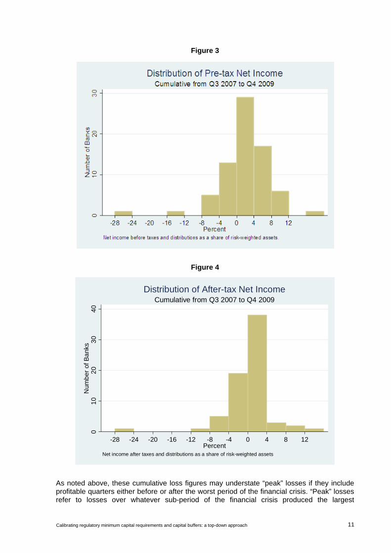
This section provides an analysis of losses by large internationally active banks during the recent financial crisis. The analysis is based on data collected for 73 banks in 14 countries. For each bank, cumulative net income over the financial crisis period (from Q3 2007 to Q4 2009) is calculated as a share of year-end 2006 risk-weighted assets. Net income is a proxy for the impact of the financial crisis on the banks’ Tier 1 capital and Tier 1 common equity in the absence of any actions by management to increase or adjust capital, such as new issuance. However, it excludes any impact on banks’ capital that is not directly reported in the income statement (eg mark-to-market variations of “available for sale” assets, which are deducted directly from capital). The analysis covers both pre-tax and after-tax net income, as well as a measure of pre-tax net income adjusted for non-recurring revenues (though it turned out that this adjustment had little effect on the results).

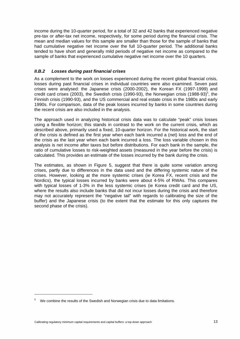
Figures 3 and 4 present the distribution of cumulative pre-tax and after-tax net income from Q3 2007 to Q4 2009 for the banks in the sample. The first result to note is that more than two-thirds of the banks had positive cumulative net income over the 10 quarters of the financial crisis (Q3 2007 to Q4 2009). Fifty-three of the 73 banks (73%) had positive net income before taxes and distributions, and 44 of 70 (63%) had positive cumulative net income after taxes and distributions. This finding may reflect differences across jurisdictions in the severity of the losses experienced during the crisis – some banks may not have experienced cumulative negative net income because the financial crisis was not overly severe in their primary areas of operation, or their business models positioned them to have more diversified earnings streams with fewer fat tail risks. It may also reflect that the loss (net income) measures are cumulative over 10 quarters, and thus the “peak” losses experienced may be masked by some profitable quarters.

Since we are interested in understanding the size of potential losses during a crisis or very stressful period, the focus of this analysis is on the negative tail of the net income distribution, that is, on the banks with negative cumulative net income. As the figures illustrate, there were about 20 such institutions. Mean losses (negative net income) equalled -4.56% of RWA for pre-tax, pre-distribution net income and -3.31% of RWA for after-tax, after-distribution net income across these institutions. The median figures are smaller, at -2.51% and -1.85% of RWA, reflecting the impact of one particularly large outlier.4 Overall, losses range between -0.60% and -25.69% of RWA for pre-tax net income and between -0.03% and -25.75% of RWA for after-tax net income.

4 The mean values excluding the outlier observation are -3.44% for pre-tax net income and -2.41% for after-tax

net income.


Figure 3

Figure 4

01

02

03

04

0N

umb

er o

f Ba

nks

-28 -24 -20 -16 -12 -8 -4 0 4 8 12Percent

Net income after taxes and distributions as a share of risk-weighted assets

Cumulative from Q3 2007 to Q4 2009Distribution of After-tax Net Income

As noted above, these cumulative loss figures may understate “peak” losses if they include profitable quarters either before or after the worst period of the financial crisis. “Peak” losses refer to losses over whatever sub-period of the financial crisis produced the largest


cumulative negative net income figure – this is a relevant concept for calibration of the supervisory buffer because it represents the largest stress that the banks in question experienced, and would therefore have required capital to absorb such losses.

To explore this idea, net income data over shorter horizons for 53 banks in ten countries is also examined. Table 1 shows the average and median values of “peak” and cumulative losses relative to RWA for banks in the ten-country sub-sample that experienced negative cumulative net income over the entire 10-quarter period. For comparison, the table also reports the average and median values of cumulative losses for the entire sample.

Average and median peak losses are markedly larger than cumulative losses over the entire 10-quarter period for these banks. Average “peak” losses on a pre-tax basis equal -5.40% of RWA, as compared to -4.36% over the entire period, and median “peak” pre-tax losses are nearly double median losses over the entire period (-3.22% of RWA, as compared to -1.67% for the entire period). The differences on an after-tax, after-distribution basis are smaller, but still distinct. In total, 13 of the 17 banks with cumulative negative pre-tax net income and 17 of the 23 banks with negative cumulative after-tax net income had “peak” losses that exceeded their cumulative losses over the full 10-quarter period. These findings suggest that data based on cumulative figures may understate realised “peak” losses for these banks. If we take results from the ten-country sample as indicative, the differences in the ratio of negative net income to RWA are on the order of 50 to 150 basis points.

Table 1

Difference between cumulative and “peak” loss rates for banks experiencing negative cumulative net income Q3 2007 – Q4 2009

Net income before taxes and distributions

Net income after taxes and distributions

Q3 2007- Q4 2009

Q3 2007- Q4 2008 “Peak”

“Peak” for all Banks

Q3 2007 - Q4 2009

Q3 2007- Q4 2008 “Peak”

“Peak” for all Banks

Ten-country sample

Average -4.36% -4.36% -5.40% -3.22% -3.08% -2.73% -3.69% -2.30%

Median -1.67% -2.10% -3.22% -2.02% -1.52% -1.75% -2.31% -0.93%

Whole sample (14 countries)

Average -4.56% n/a n/a n/a -3.31% n/a n/a n/a

Median -2.51% n/a n/a n/a -1.85% n/a n/a n/a

Figures are the average and median values of the ratio of net income to risk-weighted assets for those banks with cumulative negative net income from Q3 2007 to Q4 2009. The ten-country sample is for 53 banks. Of these, 17 had cumulative negative net income before taxes and distributions and 23 had cumulative negative net income after taxes and distributions. “Peak” values equal the largest value of cumulative negative net income over any period between Q3 2007 and Q4 2009. Figures in the columns labelled ‘ “Peak” for all Banks’ are the average and median values of “peak” losses for across all banks with negative net income for some period during Q3 2007 to Q4 2009, whether or not cumulative net income was negative over this period. In total, 32 banks had negative pre-tax net income for some period during Q3 2007 to Q4 2009 and 42 banks had negative net income after taxes and distributions for some period during this time.

The figures in the first set of columns in Table 1 are for banks with cumulative negative net income over the entire Q3 2007 to Q4 2009 period. The final column (labelled ‘ “Peak” for all Banks’) reports data for all banks in the sample that experienced negative net income at some period during this time. Overall, 15 banks with positive pre-tax cumulative net income and 19 banks with positive cumulative after tax net income had periods of negative net


income during the 10-quarter period, for a total of 32 and 42 banks that experienced negative pre-tax or after-tax net income, respectively, for some period during the financial crisis. The mean and median values for this sample are smaller than those for the sample of banks that had cumulative negative net income over the full 10-quarter period. The additional banks tended to have short and generally mild periods of negative net income as compared to the sample of banks that experienced cumulative negative net income over the 10 quarters.

II.B.2 Losses during past financial crises

As a complement to the work on losses experienced during the recent global financial crisis, losses during past financial crises in individual countries were also examined. Seven past crises were analysed: the Japanese crisis (2000-2002), the Korean FX (1997-1999) and credit card crises (2003), the Swedish crisis (1990-93), the Norwegian crisis (1988-93)5, the Finnish crisis (1990-93), and the US commercial and real estate crisis in the 1980s and early 1990s. For comparison, data of the peak losses incurred by banks in some countries during the recent crisis are also included in the analysis.

The approach used in analyzing historical crisis data was to calculate “peak” crisis losses using a flexible horizon; this stands in contrast to the work on the current crisis, which as described above, primarily used a fixed, 10-quarter horizon. For the historical work, the start of the crisis is defined as the first year when each bank incurred a (net) loss and the end of the crisis as the last year when each bank incurred a loss. The loss variable chosen in this analysis is net income after taxes but before distributions. For each bank in the sample, the ratio of cumulative losses to risk-weighted assets (measured in the year before the crisis) is calculated. This provides an estimate of the losses incurred by the bank during the crisis.

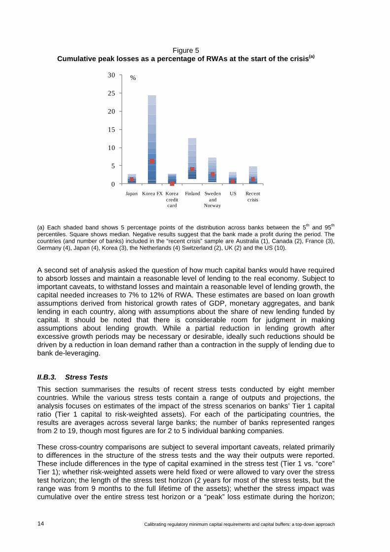
The estimates, as shown in Figure 5, suggest that there is quite some variation among crises, partly due to differences in the data used and the differing systemic nature of the crises. However, looking at the more systemic crises (ie Korea FX, recent crisis and the Nordics), the typical losses incurred by banks were about 4-5% of RWAs. This compares with typical losses of 1-3% in the less systemic crises (ie Korea credit card and the US, where the results also include banks that did not incur losses during the crisis and therefore may not accurately represent the “negative tail” with regards to calibrating the size of the buffer) and the Japanese crisis (to the extent that the estimate for this only captures the second phase of the crisis).

5 We combine the results of the Swedish and Norwegian crisis due to data limitations.


Figure 5 Cumulative peak losses as a percentage of RWAs at the start of the crisis(a)

0

5

10

15

20

25

30

Japan Korea FX Korea credit card

Finland Sweden and

Norway

US Recent crisis

%

(a) Each shaded band shows 5 percentage points of the distribution across banks between the 5th and 95th percentiles. Square shows median. Negative results suggest that the bank made a profit during the period. The countries (and number of banks) included in the “recent crisis” sample are Australia (1), Canada (2), France (3), Germany (4), Japan (4), Korea (3), the Netherlands (4) Switzerland (2), UK (2) and the US (10).

A second set of analysis asked the question of how much capital banks would have required to absorb losses and maintain a reasonable level of lending to the real economy. Subject to important caveats, to withstand losses and maintain a reasonable level of lending growth, the capital needed increases to 7% to 12% of RWA. These estimates are based on loan growth assumptions derived from historical growth rates of GDP, monetary aggregates, and bank lending in each country, along with assumptions about the share of new lending funded by capital. It should be noted that there is considerable room for judgment in making assumptions about lending growth. While a partial reduction in lending growth after excessive growth periods may be necessary or desirable, ideally such reductions should be driven by a reduction in loan demand rather than a contraction in the supply of lending due to bank de-leveraging.

II.B.3. Stress Tests

This section summarises the results of recent stress tests conducted by eight member countries. While the various stress tests contain a range of outputs and projections, the analysis focuses on estimates of the impact of the stress scenarios on banks’ Tier 1 capital ratio (Tier 1 capital to risk-weighted assets). For each of the participating countries, the results are averages across several large banks; the number of banks represented ranges from 2 to 19, though most figures are for 2 to 5 individual banking companies.

These cross-country comparisons are subject to several important caveats, related primarily to differences in the structure of the stress tests and the way their outputs were reported. These include differences in the type of capital examined in the stress test (Tier 1 vs. “core” Tier 1); whether risk-weighted assets were held fixed or were allowed to vary over the stress test horizon; the length of the stress test horizon (2 years for most of the stress tests, but the range was from 9 months to the full lifetime of the assets); whether the stress impact was cumulative over the entire stress test horizon or a “peak” loss estimate during the horizon;


the severity of the underlying stress scenario; and whether banks or supervisors made the estimates.

Some of these differences undoubtedly have a large impact on the results, though it is difficult in some cases to determine precisely the extent of the impact. In general, however, the impact on Tier 1 capital was more severe (more negative) when supervisors, as opposed to banks, made the estimates; when the impact is measured as “peak to trough” rather than cumulatively; and for longer horizons.

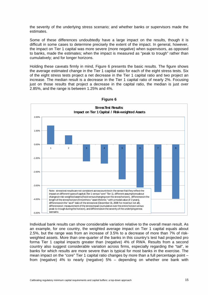
Holding these caveats firmly in mind, Figure 6 presents the basic results. The figure shows the average estimated change in the Tier 1 capital ratio for each of the eight stress tests. Six of the eight stress tests project a net decrease in the Tier 1 capital ratio and two project an increase. The median result is a decrease in the Tier 1 capital ratio of nearly 2%. Focusing just on those results that project a decrease in the capital ratio, the median is just over 2.85%, and the range is between 1.25% and 4%.

Figure 6

-5.00%

-4.00%

-3.00%

-2.00%

-1.00%

0.00%

1.00%

2.00%

1 2 3 4 5 6 7 8

Stress Test Results: Impact on Tier 1 Capital / Risk-weighted Assets

Note: stress test resultsare not consistent across countries in the sense that they reflect the impact on different types of capital (Tier 1 versus "core" Tier 1), different assumptions about changes in risk-weighted assets (fixed versus changing over the stress horizon), differences in the length of the stress horizon (9 months to "asset lifetime," with a modal value of 2 years), differences in the "as of" date of the stress test (December 31, 2008 for most but not all), differences in measurement of the stress impact (cumulative over the entire horizon versus peak-to-trough during the horizon), and differences in the severity of the underlying stress scenairio.

Individual bank results can show considerable variation relative to the overall mean result. As an example, for one country, the weighted average impact on Tier 1 capital equals about 2.5%, but the range was from an increase of 3.5% to a decrease of more than 7% of risk-weighted assets. More than one-quarter of the banks in this country’s test had projected pro forma Tier 1 capital impacts greater than (negative) 4% of RWA. Results from a second country also suggest considerable variation across firms, especially regarding the “tail”, ie banks for which results are more severe than is typical for most banks in the exercise. The mean impact on the “core” Tier 1 capital ratio changes by more than a full percentage point – from (negative) 4% to nearly (negative) 5% – depending on whether one bank with


particularly severe results was included or excluded in the mean. Finally, for a third country, individual bank results range between 1.75% and more than 5.0% of RWA.

In interpreting all these results in the context of the supervisory capital buffer, it is important to note that they do not incorporate any losses the banks may have sustained during the early part of the financial crisis, before the “as of” dates of the stress tests (which were generally year-end 2008). This could be an important omission in thinking about the total impact of the financial crisis, as losses were substantial for some (though certainly not all) institutions over this period. For instance, data from one country suggests that including pre-stress test losses increases the weighted average cumulative loss figure by 2 percentage points, from 2.5% to 4.5% of risk-weighted assets. Overall, more than a third of the banks have an implied decrease greater than 5% of RWA, when pre stress test realised results are included. Because these figures combined projected stress losses and realised actual losses, they should be viewed as peak estimates of the impact of the financial crisis on banks’ capital positions.

II.C. Leverage ratio II.C.1 Historical leverage ratios

To provide background and reference for calibration of the leverage ratio, data was also collected from 10 member countries on capital and leverage for large banks, for a period generally covering the early to mid-1990s to present. Due to lack of data and data consistency issues, the analysis focused primarily on Tier 1 capital to assets as the measure of leverage. The findings indicate that large banks have been increasing financial leverage over the sample period, with the weighted average Tier 1 leverage ratio declining from 3.5% to 2.5% over the past decade for countries that adopted IFRS in 2005, and from 7.7% to 6.4% in non-IFRS countries.

II.C.2 Discriminating between stressed and non-stressed banks

Using data collected from national supervisors, and also a large commercially available database with international coverage, analysis was undertaken to examine which ratios discriminated between stressed and non-stressed banks prior to the recent crisis, and the level of the ratio that best discriminated between the stressed and non-stressed banks. Differences in mean leverage ratios before the crisis are not directly useful for calibration, but are presented as background information.

To perform this analysis, information was collected on several types of leverage ratios for 88 banks from 14 member countries (Working Group Sample). To augment these data, a second set of data was also collected on the capital ratios for 117 large banks from 19 countries, drawing from a large commercial data base (Broader Sample). Among the banks in these samples, “stressed” banks are those that failed, were acquired under stress, or that received firm-specific government assistance.

The leverage ratios examined were the ratio of Tier 1 capital to assets, the ratio of common equity to assets, the ratio of tangible common equity (TCE) to tangible assets, and the ratio of common equity minus current Tier 1 deductions to assets.6 Of course, none of these ratios

6 For the Working Group Sample, TCE is defined as total common equity (equal to paid in shares plus retained

earnings) minus goodwill and intangibles (where intangibles are defined according to national rules). For the Broader Sample, TCE is defined as the sum of common stock, additional paid in capital, and retained earnings less the sum of treasury shares, intangibles and goodwill.


matches precisely the definitions ultimately adopted by the Basel Committee, as both the definition of capital and the definition of exposures differ (eg off-balance sheet exposures are not included in the calculation of leverage ratios shown in Table 3) so these results are merely indicative.

The results of the difference in means tests are presented in Table 2 for end 2006 data. In all cases, the mean leverage ratio of stressed banks were lower than the mean leverage ratio of non-stressed banks. In many cases, the differences in the means are statistically significant, particularly when the sample excludes banks domiciled in countries that had in place a minimum leverage ratio requirement prior to the financial crisis. Very similar results are obtained using data from 2007.7

Table 2

Mean leverage-based capital ratios for groups of stressed and non-stressed banks (Data is calculated as at end 2006)

Working Group Sample Broader Sample

Stressed Other Stressed Other Total Capital / Assets 11 6.33% 58 7.92% 19 5.50% 66 6.57% * Tier 1 Capital / Assets 11 4.38% 58 5.62% 20 3.89% 69 4.19% Common Equity / Assets 11 5.49% 58 5.76% 27 4.07% 79 5.12% Tangible Common Equity / Tangible Assets 11 3.08% 58 4.28% 27 2.65% 79 3.81% **

Excluding countries with leverage ratio requirements

Stressed Other Stressed Other Total Capital / Assets 6 4.32% 41 7.62% ** 14 4.37% 51 6.28% ***Tier 1 Capital / Assets 6 2.79% 41 5.27% ** 15 3.02% 54 3.65% * Common Equity / Assets 6 2.69% 41 5.08% ** 17 2.64% 63 4.48% ***Tangible Common Equity / Tangible Assets 6 1.93% 41 4.34% ** 17 2.22% 63 3.62% ***

The symbols ***, **, * indicate that the difference is statistically significant at the 1%, 5% and 10% levels respectively. The Working Group Sample comprises up to 88 banks supplied by national supervisors from 14 countries. The Broader Sample is drawn from the Bankscope database and includes up to 117 banks from 19 countries.

II.C.3 Critical values

The main aim of the analysis of severely stressed and other banks is to identify whether there exists a “critical value” of each ratio that distinguishes “severely stressed” from other banks. That is, for each ratio, the aim is to identify a level of the ratio such that most “severely stressed” banks had ratios below that level, and most other banks had ratios above that level. If such a critical value can be identified, then it may provide a useful benchmark for the regulatory minimum requirement since banks with ratios below that level ultimately experienced significant stress, while banks with ratios above that level experienced less

7 Using a similar analysis, there is little evidence that risk-based capital ratios were consistently higher for the

group of non-stressed banks prior to the crisis. The ratio of tangible common equity (TCE) to RWA is the only risk-based ratio for which severely stressed banks had statistically significantly lower values than non-stressed banks prior to the crisis (and only when using the Broader Sample). In this case, using end 2006 data, the mean TCE/RWA ratio for the sample of 19 stressed banks is 5.75% and 7.66% for the sample of 73 other banks.


stress. While not as direct a calibration approach as the RORWA analysis performed for the risk-based minimum requirement, the critical value analysis provides at least a rough indication of the range of leverage ratios that appear to have separated severely distressed banks before and in the early stages of the financial crisis.

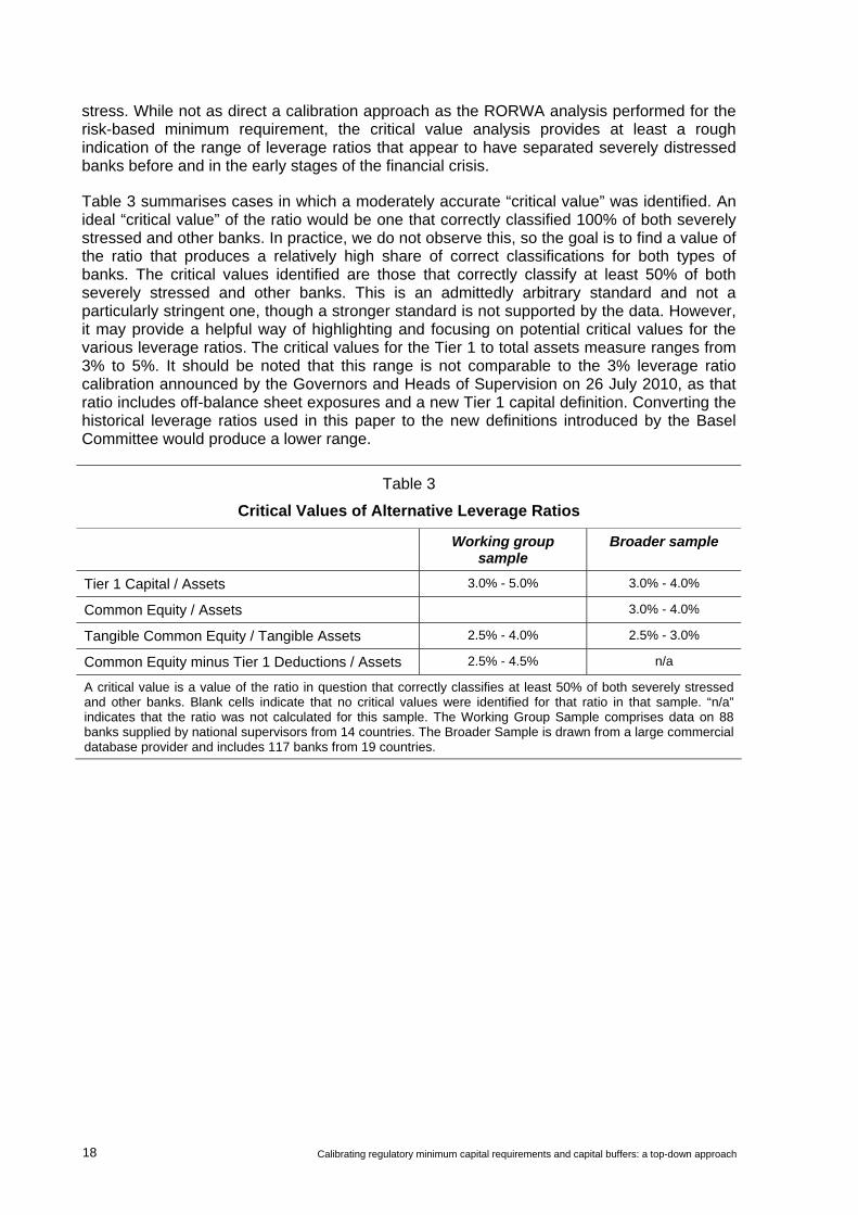
Table 3 summarises cases in which a moderately accurate “critical value” was identified. An ideal “critical value” of the ratio would be one that correctly classified 100% of both severely stressed and other banks. In practice, we do not observe this, so the goal is to find a value of the ratio that produces a relatively high share of correct classifications for both types of banks. The critical values identified are those that correctly classify at least 50% of both severely stressed and other banks. This is an admittedly arbitrary standard and not a particularly stringent one, though a stronger standard is not supported by the data. However, it may provide a helpful way of highlighting and focusing on potential critical values for the various leverage ratios. The critical values for the Tier 1 to total assets measure ranges from 3% to 5%. It should be noted that this range is not comparable to the 3% leverage ratio calibration announced by the Governors and Heads of Supervision on 26 July 2010, as that ratio includes off-balance sheet exposures and a new Tier 1 capital definition. Converting the historical leverage ratios used in this paper to the new definitions introduced by the Basel Committee would produce a lower range.

Table 3

Critical Values of Alternative Leverage Ratios

Working group sample

Broader sample

Tier 1 Capital / Assets 3.0% - 5.0% 3.0% - 4.0%

Common Equity / Assets 3.0% - 4.0%

Tangible Common Equity / Tangible Assets 2.5% - 4.0% 2.5% - 3.0%

Common Equity minus Tier 1 Deductions / Assets 2.5% - 4.5% n/a

A critical value is a value of the ratio in question that correctly classifies at least 50% of both severely stressed and other banks. Blank cells indicate that no critical values were identified for that ratio in that sample. “n/a” indicates that the ratio was not calculated for this sample. The Working Group Sample comprises data on 88 banks supplied by national supervisors from 14 countries. The Broader Sample is drawn from a large commercial database provider and includes 117 banks from 19 countries.


Working group members

Chair Ms Beverly Hirtle

Australia Mr Charles Littrell

Brazil Mr Caio Fonseca Ferreira

Canada Mr Richard Gresser

China Mr Shengbang Wang

France Mr Dominique Laboureix Mr Philippe Mongars

Germany Mr Klaus Düllmann

Italy Mr Francesco Cannata

Japan Mr Koga Sawada Mr Isao Yoshitomi

Korea Mr Byungchil Kim

Netherlands Ms Sandra Wesseling

Spain Ms Linette Field

Switzerland Mr Bertrand Rime Mr Daniel Sigrist

United Kingdom Mr Duncan MacKinnon Mr Sujit Kapadia

United States Mr Francisco Covas Mr George French Mr David Jones Ms Andrea Plante Mr Mark Levonian

European Commission Mr Andreas Strohm

Secretariat Mr Neil Esho