1
CENTRE FOR EMEA BANKING, FINANCE & ECONOMICS
Modelling and Trading the Greek Stock Market with
Mixed Neural Network Models
Christian L. Dunis
Jason Laws
Andreas Karathanasopoulos
Working Paper Series
No 15/11

2
Modelling and Trading
the Greek Stock Market with Mixed Neural Network Models
Christian L. Dunis*
Jason Laws
Andreas Karathanasopoulos
Abstract
In this paper, a mixed methodology that combines both the ARMA and NNR models is
proposed to take advantage of the unique strength of ARMA and NNR models in linear
and nonlinear modelling. Experimental results with real data sets indicate that the
combined model can be an effective way to improve forecasting accuracy achieved by
either of the models used separately. The motivation for this paper is to investigate the
use of alternative novel neural network architectures when applied to the task of
forecasting and trading the ASE 20 Greek Index using only autoregressive terms as
inputs. This is done by benchmarking the forecasting performance of six different neural
network designs representing a Higher Order Neural Network (HONN), a Recurrent
Network (RNN), a classic Multilayer Percepton (MLP), a Mixed Higher Order Neural
Network, a Mixed Recurrent Neural Network and a Mixed Multilayer Percepton Neural
Network with some traditional techniques, either statistical such as a an autoregressive
moving average model (ARMA), or technical such as a moving average
convergence/divergence model (MACD), plus a naïve trading strategy. More specifically,
the trading performance of all models is investigated in a forecast and trading simulation
on ASE 20 fixing time series over the period 2001-2008 using the last one and a half
year for out-of-sample testing. We use the ASE 20 daily fixing as many financial
institutions are ready to trade at this level and it is therefore possible to leave orders with
a bank for business to be transacted on that basis.
____________
Christian Dunis is Professor of Banking and Finance at Liverpool Business School and
Director of the Centre for International Banking, Economics and Finance (CIBEF) at Liverpool John
Moores University (E-mail: [email protected]).
Jason Laws is Reader of Finance at Liverpool Business School and a member of CIBEF (E-mail:
Andreas Karathanasopoulos is Senior Lecturer at London Metropolitan Business School(E-mail:

3
1. INTRODUCTION
The use of intelligent systems for market predictions has been widely established. This
paper deals with the application of mixed computing techniques for forecasting the
Greek stock market. The development of accurate techniques is critical to economists,
investors and analysts. This task is getting more and more complex as financial markets
are getting increasingly interconnected and interdependent. The traditional statistical
methods, on which forecasters were reliant in recent years, seem to fail to capture the
interrelationship between market variables. This paper investigates methods capable of
identifying and capturing all the discontinuities, the nonlinearities and the high frequency
multipolynomial components characterizing the financial series today. A model category
that promises such effective results is the combination of autoregressive models such as
ARMA model with Neural Networks named Mixed-Neural Network model. Many
researchers have argued that combining several models for forecasting gives better
estimates by taking advantage of each model’s capabilities when comparing them with
single time series models.
The motivation for this paper is to investigate the use of several new neural networks
techniques combined with ARMA model in order to overcome these limitations using
autoregressive terms as inputs. This is done by benchmarking six different neural
network architectures representing a Multilayer Percepton (MLP), a Higher Order Neural
Network (HONN), a Recurrent Neural Network (RNN), a Mixed Higher order Neural
Network, a Mixed Recurrent Neural Network and a Mixed Multilayer Percepton Neural
Network Their trading performance on the ASE 20 time series is investigated and is
compared with some traditional statistical or technical methods such as an
autoregressive moving average (ARMA) model or a moving average
convergence/divergence (MACD) model, and a naïve trading strategy.
As it turns out, the Mixed-HONN demonstrates a remarkable performance and
outperforms all other models in a simple trading simulation exercise. On the other hand,
when more sophisticated trading strategies using confirmation filters and leverage are
applied, Mixed MLPs outperform all models in terms of annualised return. Our
conclusion colloborates those of Lindemann et al. (2004) and Dunis et al. (2008b) where
HONNs also demonstrate a forecasting superiority on the EUR/USD series over more
traditional techniques such as a MACD and a naïve strategy. However, the RNN which
performed remarkably well, show a disappointing performance in this research: this may
be due to their inability to provide good enough results when only autoregressive terms
are used as inputs.
The rest of the paper is organised as follows. In section 2, we present the literature
relevant to the Mixed Neural Networks, the Recurrent Neural Network, the Higher Order
4
Neural Networks and the Multilayer Percepton. Section 3 describes the dataset used for
this research and its characteristics. An overview of the different neural network models
and statistical techniques is given in section 4. Section 5 gives the empirical results of all
the models considered and investigates the possibility of improving their performance
with the application of more sophisticated trading strategies. Section 6 provides some
concluding remarks.
2. LITERATURE REVIEW
Stock market analysis is an area of financial application. Detecting trends of stock
market data is a difficult task as they have complex, nonlinear, dynamic and chaotic
behaviour. Time series methods such as ARMA model and autoregressive conditional
heteroskedasticity models are not capable of accurately forecasting the time series as
they are based on the theory of stationary stochastic processes. Empirical studies prove
that artificial Neural Networks models perform better than these time series models.
Ghiassi et al. (2005) compare forecasting performance of a dynamic Neural Network
with traditional neural networks and ARMA models. Greg and Sarah (1999) use Neural
Networks for GDP growth and determined whether the forecasting performance of
financial and monetary variables can be improved using Neural Networks. Fatima and
Hussain (2008) propose a Hybrid financial system that in terms of forecasting behaves
better compared to standard models.
The motivation for this paper is to apply some of the most promising new Neural
Networks architectures combining them with autoregressive models (in our case ARMA
model) which have been developed recently with the purpose to overcome the
numerous limitations of the more classic neural architectures and to assess whether
they can achieve a higher performance in a trading simulation using only autoregressive
series as inputs.
Combining different models can increase the chance to capture different patterns in the
data and improve forecasting performance. Several empirical studies have already
suggested that by combining several different models, forecasting accuracy can often be
improved over an individual model. Using hybrid models or combining several models
has become a common practice to improve the forecasting accuracy since the well-
known M-competition (Makridakis et al.(1982)) in which combinations of forecasts from
more than one model often led to improved forecasting performance. The basic idea of
the model combination in forecasting is to use each model’s unique feature to capture
different patterns in the data. Both theoretical and empirical findings suggest that
combining different methods can be an effective and efficient way to improve forecasts
5
(Makridakis (1989), Newbold et al. (1974) Palm et al. (1992), Winkler (1989)). Research
in time series forecasting argues that predictive performance improves the combined
models. (Bishop (1994), Clemen (1989), Hansen et al. (2003), Hibbert et al. (2000),
Terui et al. (2002), Tseng et al. (2002), Zhang, (2003), Zhang et al. (2005)).
The reason for combining models comes from the assumption that either one cannot
identify the true data generating process (Terui and Von Dyke. (2002)) or that a single
model may not be sufficient to identify all the characteristics of the time series (Zhang
(2003)). Moreover the use of hybrid neural network has not been used until the moment
that scientists started to investigate not only the benefits of Hybrid Neural Networks
against other statistical methods but also the differences between different combinations
of Hybrid Neural Networks with other statistical models following the Hybrid GARCH-NN
approach Wang (2007) and the Hybrid ARIMA/ ARCH-NN of Fatima and Hussain
(2008). Abraham et al. (2002) analysed the 24-month stock data for NASDAQ-100 main
indices. Their hybrid system is Neuro-Fuzzy, a combination of neural network and fuzzy
logic system. Lastly Andreou et al. (2006) propose knowledge-oriented neural network
models combining nonparametric with parametric models (Black –Scholes) for option
price data.
RNNs have an activation feedback which embodies short-term memory allowing them to
learn extremely complex temporal patterns. Their superiority against feedfoward
networks when performing nonlinear time series prediction is well documented in
Connor et al. (1993) and Adam et al. (1994). In financial applications, Kamijo et al.
(1990) applied them successfully to the recognition of stock patterns of the Tokyo stock
exchange while Tenti (1996) achieved remarkable results using RNNs to forecast the
exchange rate of the Deutsche Mark. Tino et al. (2001) use them to trade successfully
the volatility of the DAX and the FTSE 100 using straddles while Dunis and Huang
(2002), using continuous implied volatility data from the currency options market, obtain
remarkable results for their GBP/USD and USD/JPY exchange rate volatility trading
simulation.
HONNs were first introduced by introduced by Giles and Maxwell (1987) as a fast
learning network with increased learning capabilities. Although their function
approximation superiority over the more traditional architectures is well documented in
the literature (see among others Redding et al. (1993), Kosmatopoulos et al. (1995) and
Psaltis et al. (1998)), their use in finance so far has been limited. This has changed
when scientists started to investigate not only the benefits of Neural Networks (NNs)
against the more traditional statistical techniques but also the differences between the
different NNs model architectures. Practical applications have now verified the
theoretical advantages of HONNs by demonstrating their superior forecasting ability and

6
put them in the front line of research in financial forecasting. For example Dunis et al.
(2006b) use them to forecast successfully the gasoline crack spread while Fultcher et al.
(2006) apply HONNs to forecast the AUD/USD exchange rate, achieving a 90%
accuracy. However, Dunis et al. (2006a) show that, in the case of the futures spreads
and for the period under review, the MLPs performed better compared with HONNs and
recurrent neural networks. Moreover, Dunis et al. (2008a), who also study the EUR/USD
series for a period of 10 years, demonstrate that when multivariate series are used as
inputs the HONNs, RNN and MLP networks have a similar forecasting power. Finally,
Dunis et al. (2008b) in a paper with a methodology identical to that used in this research,
demonstrate that HONN and the MLP networks are superior in forecasting the
EUR/USD ECB fixing until the end of 2007, compared to the RNN networks, an ARMA
model, a MACD and a naïve strategy.
3. THE ASE 20 GREEK INDEX AND RELATED FINANCIAL DATA
For Futures on the FTSE/ASE-20 that are traded in derivatives markets the underlying
asset is the blue chip index FTSE/ASE-20. The FTSE/ASE-20 index is based on the 20
largest ASE stocks. It was developed in 1997 by the partnership of ASE with FTSE
International and is already established benchmark. It represents over 50% of ASE's
total capitalisation and currently has a heavier weight on banking, telecommunication
and energy stocks.
The futures contract on the index FTSE/ASE-20 is cash settled in the sense that the
difference between the traded price of the contract and the closing price of the index on
the expiration day of the contract is settled between the counterparties in cash. As a
matter of fact, as the price of the contract changes daily, it is cash settled on a daily
basis, up until the expiration of the contract.
The futures contract is traded in index points, while the monetary value of the contract is
calculated by multiplying the futures price by the multiplier 5 EUR per point. For
example, a contract trading at 1,400 points has a value of 7,000 EUR.
The ASE 20 Futures is therefore a tradable level which makes our application more
realistic and this is the series that we investigate in this paper1.
Name of Period Trading Days Beginning End
Total Dataset 2087 21 January 2001 31 December 2008
Training Dataset 1719 29 January 2001 30 August 2007
Out- of- sample Dataset(Validation Set) 349 31 August /2007 31 December 2008
1 We examine the ASE 20 since its first trading day on 21 January 2001, and until 31 December 2008,
using the continuous data available from datastream.

Fig. 1
The observed ASE 20 time series is non
the 99% confidence interval) containing slight skewness and high kurtosis. It is also
non-stationary and we decided to transform the ASE 20 series into stationary series of
rates of return2.
Given the price level P1, P2,…,
2 Confirmation of its stationary property is obtained at the 1% significance level by both the Augmented
Dickey Fuller (ADF) and Phillips-
7
Table 1: The ASE 20 dataset
Fig. 1: ASE 20 fixing prices (total dataset).
The observed ASE 20 time series is non-normal (Jarque-Bera statistics confirms
the 99% confidence interval) containing slight skewness and high kurtosis. It is also
stationary and we decided to transform the ASE 20 series into stationary series of
,…,Pt, the rate of return at time t is formed by:
11
−
=
−t
t
tP
PR
Confirmation of its stationary property is obtained at the 1% significance level by both the Augmented
-Perron (PP) test statistics.
statistics confirms this at
the 99% confidence interval) containing slight skewness and high kurtosis. It is also
stationary and we decided to transform the ASE 20 series into stationary series of
is formed by:
[1]
Confirmation of its stationary property is obtained at the 1% significance level by both the Augmented
8
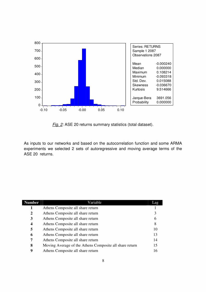
Fig. 2: ASE 20 returns summary statistics (total dataset).
As inputs to our networks and based on the autocorrelation function and some ARMA
experiments we selected 2 sets of autoregressive and moving average terms of the
ASE 20 returns.
Number Variable Lag
1 Athens Composite all share return 1
2 Athens Composite all share return 3
3 Athens Composite all share return 6
4 Athens Composite all share return 8
5 Athens Composite all share return 10
6 Athens Composite all share return 13
7 Athens Composite all share return 14
8 Moving Average of the Athens Composite all share return 15
9 Athens Composite all share return 16
0
100
200
300
400
500
600
700
800
-0.10 -0.05 -0.00 0.05 0.10
Series: RETURNS
Sample 1 2087
Observations 2087
Mean -0.000240
Median 0.000000
Maximum 0.108214
Minimum -0.093318
Std. Dev. 0.015088
Skewness -0.036670
Kurtosis 9.514666
Jarque-Bera 3691.056
Probability 0.000000

9
10 Athens Composite all share return 18
11 Moving Average of the Athens Composite all share return 19
Table 2: Explanatory variables for traditional Neural Networks
Number Variable Lag
1 Athens Composite all share return 1
2 Athens Composite all share return 2
3 Athens Composite all share return 4
4 Athens Composite all share return 5
5 Athens Composite all share return 7
6 Athens Composite all share return 9
7 Moving Average of the Athens Composite all share return 10
8 Athens Composite all share return 13
9 Athens Composite all share return 14
10 Athens Composite all share return 15
11 Moving Average of the Athens Composite all share return 16
12 Athens Composite all share return 17
Table 3: Explanatory variables for Mixed Neural Networks
In order to train the neural networks we further divided our dataset as follows:
Name of Period Trading Days Beginning End
Total Dataset 2087 21 January 2001 31 December 2008
Training Dataset 1373 29 January 2001 03 May2006
Test Dataset 346 04 May 2006 30 August 2007
Out-of- sample Dataset (Validation Set) 349 31 August 2007 31 December 2008
Table 4: The Neural Networks datasets
4. FORECASTING MODELS
4.1 Benchmark Models

10
In this paper, we benchmark our neural network models with 3 traditional strategies,
namely an autoregressive moving average model (ARMA), a moving average
convergence/divergence technical model (MACD) and a naïve strategy.
4.1.1 Naïve strategy
The naïve strategy simply takes the most recent period change as the best prediction of
the future change. The model is defined by:
tt YY =+1
ˆ [2]
Where tY is the actual rate of return at period t
1ˆ
+tY is the forecast rate of return for the next period
The performance of the strategy is evaluated in terms of trading performance via a
simulated trading strategy.
4.1.2 Moving Average
The moving average model is defined as:
( )n
YYYYM ntttt
t
121 ... +−−− ++++= [3]
Where tM is the moving average at time t
n is the number of terms in the moving average
tY is the actual rate of return at period t
The MACD strategy used is quite simple. Two moving average series are created with
different moving average lengths. The decision rule for taking positions in the market is
straightforward. Positions are taken if the moving averages intersect. If the short-term
moving average intersects the long-term moving average from below a ‘long’ position is
taken. Conversely, if the long-term moving average is intersected from above a ‘short’
position is taken3.
The forecaster must use judgement when determining the number of periods n on which
to base the moving averages. The combination that performed best over the in-sample
sub-period was retained for out-of-sample evaluation. The model selected was a
combination of the ASE 20 and its 7-day moving average, namely n = 1 and 7
respectively or a (1, 7) combination. The performance of this strategy is evaluated solely
in terms of trading performance.
3A ‘long’ ASE 20 position means buying the index at the current price, while a ‘short’ position means
selling the index at the current price.
11
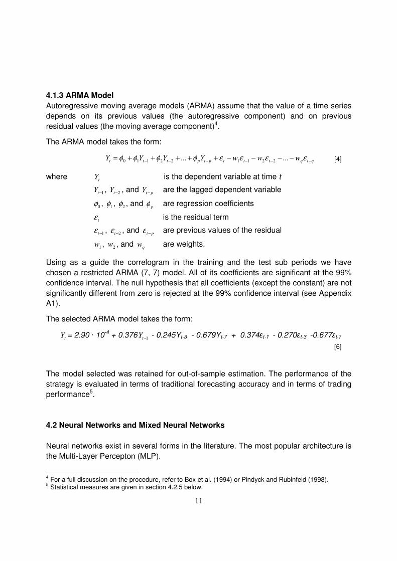
4.1.3 ARMA Model
Autoregressive moving average models (ARMA) assume that the value of a time series
depends on its previous values (the autoregressive component) and on previous
residual values (the moving average component)4.
The ARMA model takes the form:
qtqtttptpttt wwwYYYY −−−−−− −−−−+++++= εεεεφφφφ ...... 221122110 [4]
where tY is the dependent variable at time t
1−tY , 2−tY , and ptY − are the lagged dependent variable
0φ , 1φ , 2φ , and pφ are regression coefficients
tε is the residual term
1−tε , 2−tε , and
pt−ε are previous values of the residual
1w , 2w , and qw are weights.
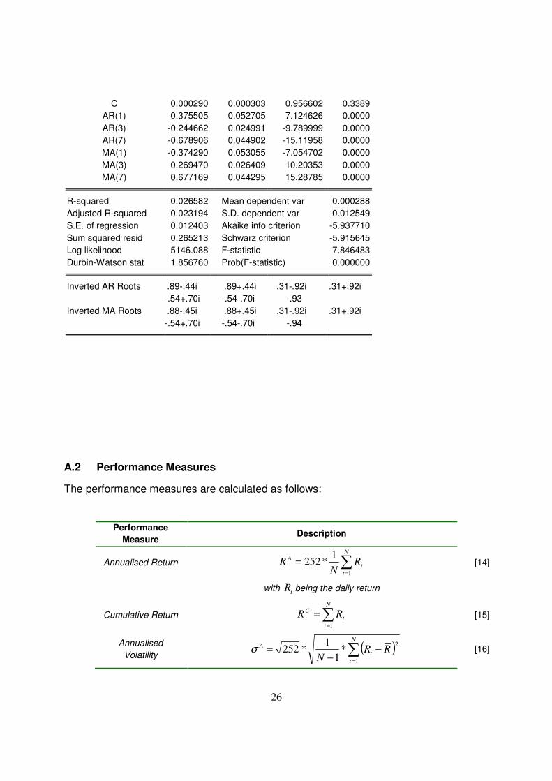
Using as a guide the correlogram in the training and the test sub periods we have
chosen a restricted ARMA (7, 7) model. All of its coefficients are significant at the 99%
confidence interval. The null hypothesis that all coefficients (except the constant) are not
significantly different from zero is rejected at the 99% confidence interval (see Appendix
A1).
The selected ARMA model takes the form:
tY = 2.90 · 10-4 + 0.3761−tY - 0.245Yt-3 - 0.679Yt-7 + 0.374εt-1 - 0.270εt-3 -0.677εt-7
[6]
The model selected was retained for out-of-sample estimation. The performance of the
strategy is evaluated in terms of traditional forecasting accuracy and in terms of trading
performance5.
4.2 Neural Networks and Mixed Neural Networks
Neural networks exist in several forms in the literature. The most popular architecture is
the Multi-Layer Percepton (MLP).
4 For a full discussion on the procedure, refer to Box et al. (1994) or Pindyck and Rubinfeld (1998).
5 Statistical measures are given in section 4.2.5 below.

12
A standard neural network has at least three layers. The first layer is called the input
layer (the number of its nodes corresponds to the number of explanatory variables). The
last layer is called the output layer (the number of its nodes corresponds to the number
of response variables). An intermediary layer of nodes, the hidden layer, separates the
input from the output layer. Its number of nodes defines the amount of complexity the
model is capable of fitting. In addition, the input and hidden layer contain an extra node,
called the bias node. This node has a fixed value of one and has the same function as
the intercept in traditional regression models. Normally, each node of one layer has
connections to all the other nodes of the next layer.
The network processes information as follows: the input nodes contain the value of the
explanatory variables. Since each node connection represents a weight factor, the
information reaches a single hidden layer node as the weighted sum of its inputs. Each
node of the hidden layer passes the information through a nonlinear activation function
and passes it on to the output layer if the calculated value is above a threshold.
The training of the network (which is the adjustment of its weights in the way that the
network maps the input value of the training data to the corresponding output value)
starts with randomly chosen weights and proceeds by applying a learning algorithm
called backpropagation of errors6 (Shapiro (2000)). The learning algorithm simply tries
to find those weights which minimize an error function (normally the sum of all squared
differences between target and actual values). Since networks with sufficient hidden
nodes are able to learn the training data (as well as their outliers and their noise) by
heart, it is crucial to stop the training procedure at the right time to prevent overfitting
(this is called ‘early stopping’). This can be achieved by dividing the dataset into 3
subsets respectively called the training and test sets used for simulating the data
currently available to fit and tune the model and the validation set used for simulating
future values. The network parameters are then estimated by fitting the training data
using the above mentioned iterative procedure (backpropagation of errors). The iteration
length is optimised by maximising the forecasting accuracy for the test dataset. Our
networks, which are specially designed for financial purposes, will stop training when
the profit of our forecasts in the test sub-period is maximized. Then the predictive value
of the model is evaluated applying it to the validation dataset (out-of-sample dataset).
There is a range of combination techniques that can be applied to forecasting the
attempt to overcome some deficiencies of single models. The combining method aims at
reducing the risk of using an inappropriate model by combining several to reduce the
6Backpropagation networks are the most common multi-layer networks and are the most commonly used
type in financial time series forecasting (Kaastra and Boyd (1996)).

13
risk of failure. Typically this is done because the underlying process cannot easily be
determined (Hibon et al. (2005)).
Combining methods involves using several redundant models designed for the same
function, where the diversity of the components is to be thought important (Brown et al.
2005). The procedure of making a mixed forecasting time series model can be achieved
by combining an ARMA process in order to learn the linear component of the conditional
mean pattern with an Artificial Neural Network process designed to learn its nonlinear
elements. The construction of the Mixed ARMA-Neural Network model is detailed is in
figure 6 below.
4.2.1 THE MULTI-LAYER PERCEPTON MODEL ARCHITECTURE
The network architecture of a ‘standard’ MLP looks as presented in figure 47:
7 The bias nodes are not shown here for the sake of simplicity.
MLP
][k
tx ][ j
th
jku
jw
ty~

14
Fig. 3: A single output, fully connected MLP model
Where: ][n
tx ( )1,,2,1 += kn L are the model inputs (including the input bias node) at time t
][m
th ( )1,...,2,1 += jm are the hidden nodes outputs (including the hidden bias node)
ty~ is the MLP model output
jku and jw are the network weights
is the transfer sigmoid function: ( )xe
xS−+
=1
1, [6]
is a linear function: ( ) ∑=i
ixxF [7]
The error function to be minimised is:
( ) ( )( )∑=
−=T
t
jjkttjjk wuyyT
wuE1
2,~1
, , with ty being the target value [8]
4.2.2 THE RECURRENT NETWORK ARCHITECTURE
Our next model is the recurrent neural network. While a complete explanation of RNN
models is beyond the scope of this paper, we present below a brief explanation of the
significant differences between RNN and MLP architectures. For an exact specification
of the recurrent network, see Elman (1990).
A simple recurrent network has activation feedback, which embodies short-term
memory. The advantages of using recurrent networks over feedforward networks, for
modelling non-linear time series, has been well documented in the past. However as
described in Tenti (1996) “the main disadvantage of RNNs is that they require
substantially more connections, and more memory in simulation, than standard
backpropagation networks”, thus resulting in a substantial increase in computational

15
time. However having said this RNNs can yield better results in comparison to simple
MLPs due to the additional memory inputs.
A simple illustration of the architecture of an Elman RNN is presented below.
Fig. 4: Elman Recurrent neural network architecture with two nodes on the hidden layer
Where:
][n
tx ( )1,,2,1 += kn L , ]2[]1[
, tt uu are the model inputs (including the input bias node) at
time t
ty~ is the recurrent model output
][ f
td )2,1( =f and][n
tw ( )1,,2,1 += kn L are the network weights
][ f
tU )2,1( =f is the output of the hidden nodes at time t
is the transfer sigmoid function: ( )xe
xS−+
=1
1, [9]
is the linear output function: ( ) ∑=i
ixxF [10]
ty~
]2[
jU
]1[
jU
]1[
jx
]2[
jx
]3[
jx
]1[
1−jU
]2[
1−jU

16
The error function to be minimised is:
( ) ( )( )∑=
−=T
t
tttttt wdyyT
wdE1
2,~1
, [11]
In short, the RNN architecture can provide more accurate outputs because the inputs
are (potentially) taken from all previous values (see inputs ]1[
1−jU and ]2[
1−jU in the figure
above).
4.2.3 THE HIGHER ORDER NEURAL NETWORK ARCHITECTURE
Higher Order Neural Networks (HONNs) were first introduced by Giles and Maxwell
(1987) and were called “Tensor Networks”. Although the extent of their use in finance
has so far been limited, Knowles et al. (2009) show that, with shorter computational
times and limited input variables, “the best HONN models show a profit increase over
the MLP of around 8%” on the EUR/USD time series (p. 7). For Zhang et al. (2002), a
significant advantage of HONNs is that “HONN models are able to provide some
rationale for the simulations they produce and thus can be regarded as “open box”
rather then “black box”. HONNs are able to simulate higher frequency, higher order non-
linear data, and consequently provide superior simulations compared to those produced
by ANNs (Artificial Neural Networks)” (p. 188). Furthermore HONNs clearly outperform
in terms of annualised return and this enables Dunis et al. (2008) to conclude with
confidence over their forecasting superiority and their stability and robustness through
time.
While they have already experienced some success in the field of pattern recognition
and associative recall8, HONNs have only started recently to be used in finance. The
architecture of a three input second order HONN is shown below:
8 Associative recall is the act of associating two seemingly unrelated entities, such as smell and colour.
For more information see Karayiannis et al. (1994).

17
Fig. 5: Left, MLP with three inputs and two hidden nodes; right, second order HONN
with three inputs
Where: ][n
tx ( )1,,2,1 += kn L are the model inputs (including the input bias node) at time t
ty~ is the HONNs model output
jku are the network weights
are the model inputs.
is the transfer sigmoid function: ( )x
exS
−+
=1
1, [12]
is a linear function: ( ) ∑=i
ixxF [13]
The error function to be minimised is:
( ) ( )( )∑=
−=T
t
jkttjjk uyyT
wuE1
2,~1
, , with ty being the target value [14]
HONNs use joint activation functions; this technique reduces the need to establish the
relationships between inputs when training. Furthermore this reduces the number of free
weights and means that HONNS are faster to train than even MLPs. However because
the number of inputs can be very large for higher order architectures, orders of 4 and
over are rarely used.
18
Another advantage of the reduction of free weights means that the problems of
overfitting and local optima affecting the results of neural networks can be largely
avoided. For a complete description of HONNs see Knowles et al. (2005).
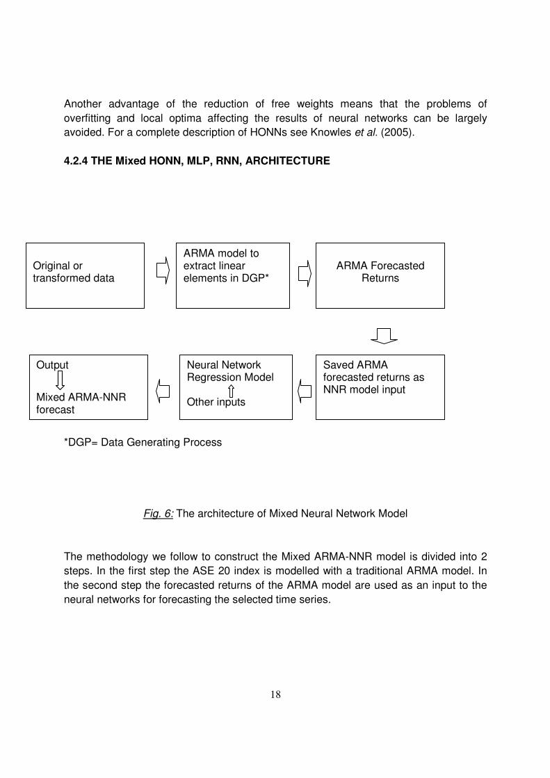
4.2.4 THE Mixed HONN, MLP, RNN, ARCHITECTURE
*DGP= Data Generating Process
Fig. 6: The architecture of Mixed Neural Network Model
The methodology we follow to construct the Mixed ARMA-NNR model is divided into 2
steps. In the first step the ASE 20 index is modelled with a traditional ARMA model. In
the second step the forecasted returns of the ARMA model are used as an input to the
neural networks for forecasting the selected time series.
ARMA model to extract linear elements in DGP*
Original or transformed data
ARMA Forecasted Returns
Saved ARMA forecasted returns as NNR model input
Neural Network Regression Model Other inputs
Output
Mixed ARMA-NNR forecast
19
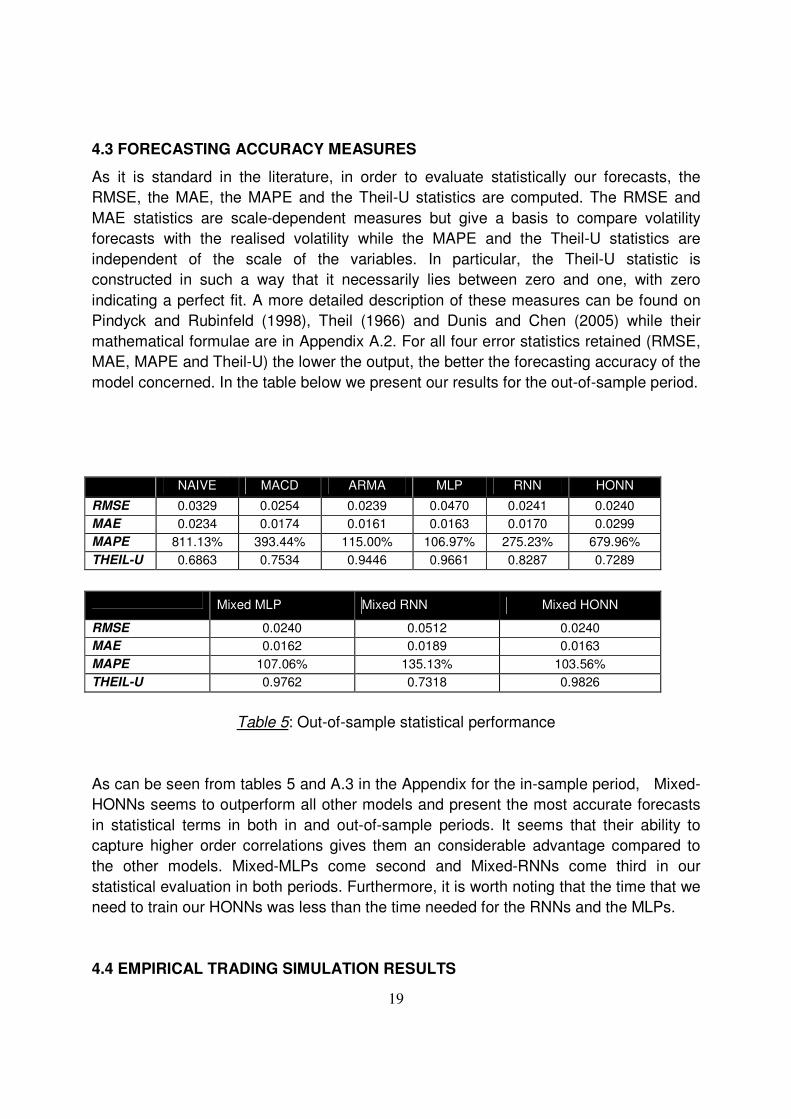
4.3 FORECASTING ACCURACY MEASURES
As it is standard in the literature, in order to evaluate statistically our forecasts, the
RMSE, the MAE, the MAPE and the Theil-U statistics are computed. The RMSE and
MAE statistics are scale-dependent measures but give a basis to compare volatility
forecasts with the realised volatility while the MAPE and the Theil-U statistics are
independent of the scale of the variables. In particular, the Theil-U statistic is
constructed in such a way that it necessarily lies between zero and one, with zero
indicating a perfect fit. A more detailed description of these measures can be found on
Pindyck and Rubinfeld (1998), Theil (1966) and Dunis and Chen (2005) while their
mathematical formulae are in Appendix A.2. For all four error statistics retained (RMSE,
MAE, MAPE and Theil-U) the lower the output, the better the forecasting accuracy of the
model concerned. In the table below we present our results for the out-of-sample period.
NAIVE MACD ARMA MLP RNN HONN
RMSE 0.0329 0.0254 0.0239 0.0470 0.0241 0.0240
MAE 0.0234 0.0174 0.0161 0.0163 0.0170 0.0299
MAPE 811.13% 393.44% 115.00% 106.97% 275.23% 679.96%
THEIL-U 0.6863 0.7534 0.9446 0.9661 0.8287 0.7289
Mixed MLP Mixed RNN Mixed HONN
RMSE 0.0240 0.0512 0.0240
MAE 0.0162 0.0189 0.0163
MAPE 107.06% 135.13% 103.56%
THEIL-U 0.9762 0.7318 0.9826
Table 5: Out-of-sample statistical performance
As can be seen from tables 5 and A.3 in the Appendix for the in-sample period, Mixed-
HONNs seems to outperform all other models and present the most accurate forecasts
in statistical terms in both in and out-of-sample periods. It seems that their ability to
capture higher order correlations gives them an considerable advantage compared to
the other models. Mixed-MLPs come second and Mixed-RNNs come third in our
statistical evaluation in both periods. Furthermore, it is worth noting that the time that we
need to train our HONNs was less than the time needed for the RNNs and the MLPs.
4.4 EMPIRICAL TRADING SIMULATION RESULTS
20
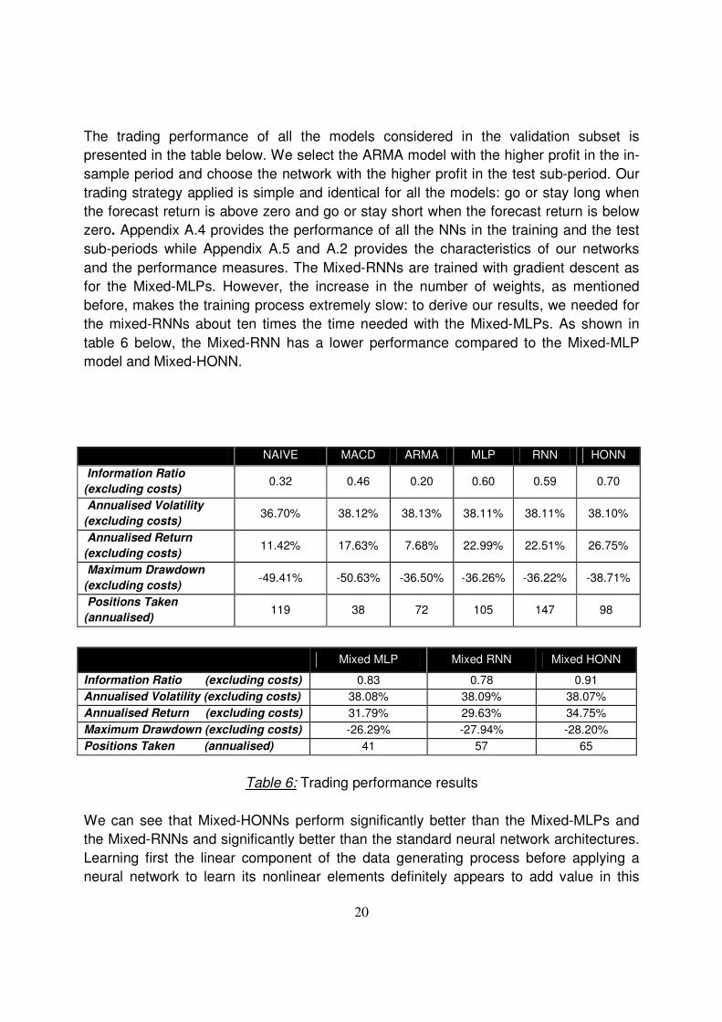
The trading performance of all the models considered in the validation subset is
presented in the table below. We select the ARMA model with the higher profit in the in-
sample period and choose the network with the higher profit in the test sub-period. Our
trading strategy applied is simple and identical for all the models: go or stay long when
the forecast return is above zero and go or stay short when the forecast return is below
zero. Appendix A.4 provides the performance of all the NNs in the training and the test
sub-periods while Appendix A.5 and A.2 provides the characteristics of our networks
and the performance measures. The Mixed-RNNs are trained with gradient descent as
for the Mixed-MLPs. However, the increase in the number of weights, as mentioned
before, makes the training process extremely slow: to derive our results, we needed for
the mixed-RNNs about ten times the time needed with the Mixed-MLPs. As shown in
table 6 below, the Mixed-RNN has a lower performance compared to the Mixed-MLP
model and Mixed-HONN.
NAIVE MACD ARMA MLP RNN HONN
Information Ratio
(excluding costs) 0.32 0.46 0.20 0.60 0.59 0.70
Annualised Volatility
(excluding costs) 36.70% 38.12% 38.13% 38.11% 38.11% 38.10%
Annualised Return
(excluding costs) 11.42% 17.63% 7.68% 22.99% 22.51% 26.75%
Maximum Drawdown
(excluding costs) -49.41% -50.63% -36.50% -36.26% -36.22% -38.71%
Positions Taken
(annualised) 119 38 72 105 147 98
Table 6: Trading performance results
We can see that Mixed-HONNs perform significantly better than the Mixed-MLPs and
the Mixed-RNNs and significantly better than the standard neural network architectures.
Learning first the linear component of the data generating process before applying a
neural network to learn its nonlinear elements definitely appears to add value in this
Mixed MLP Mixed RNN Mixed HONN
Information Ratio (excluding costs) 0.83 0.78 0.91
Annualised Volatility (excluding costs) 38.08% 38.09% 38.07%
Annualised Return (excluding costs) 31.79% 29.63% 34.75%
Maximum Drawdown (excluding costs) -26.29% -27.94% -28.20%
Positions Taken (annualised) 41 57 65
21
application. Comparing the recent paper of Dunis et al. (2010a) we notice that Hybrid-
NNR models outperform in terms of information ratio Mixed-NNR models. However
much higher drawdowns, possibly linked to the higher trading frequency of the Hybrid
models compared with the mixed models presented here.
5. TRADING COSTS AND LEVERAGE
Up to now, we have presented the trading results of all our models without considering
transaction costs. Since some of our models trade quite often, taking transaction costs
into account might change the whole picture. Following Dunis et al. (2008a), we check
for potentional improvements to our models through the application of confirmation
filters. Confirmation filters are trading strategies devised to filter out those trades with
expected returns below a threshold d around zero. They suggest to go long when the
forecast is above d and to go short when the forecast is below d. It just so happens that
the Mixed ARMA-Neural Network models perform best without any filter. This is also the
case of the MLP and HONN models. Still, the application of confirmation filters to the
benchmark models and the RNN model could have led to these models outperforming
the Mixed, MLP HONN models. This is not the case in order to conserve space, these
results are not shown here but they are available from the authors.
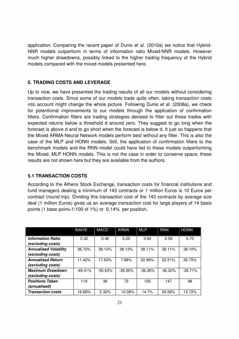
5.1 TRANSACTION COSTS
According to the Athens Stock Exchange, transaction costs for financial institutions and
fund managers dealing a minimum of 143 contracts or 1 million Euros is 10 Euros per
contract (round trip). Dividing this transaction cost of the 143 contracts by average size
deal (1 million Euros) gives us an average transaction cost for large players of 14 basis
points (1 base point=1/100 of 1%) or 0.14% per position.
NAIVE MACD ARMA MLP RNN HONN
Information Ratio
(excluding costs)
0.32 0.46 0.20 0.60 0.59 0.70
Annualised Volatility
(excluding costs)
36.70% 38.12% 38.13% 38.11% 38.11% 38.10%
Annualised Return
(excluding costs)
11.42% 17.63% 7.68% 22.99% 22.51% 26.75%
Maximum Drawdown
(excluding costs)
-49.41% -50.63% -36.50% -36.26% -36.22% -38.71%
Positions Taken
(annualised)
119 38 72 105 147 98
Transaction costs 16.66% 5.32% 10.08% 14.7% 20.58% 13.72%
22
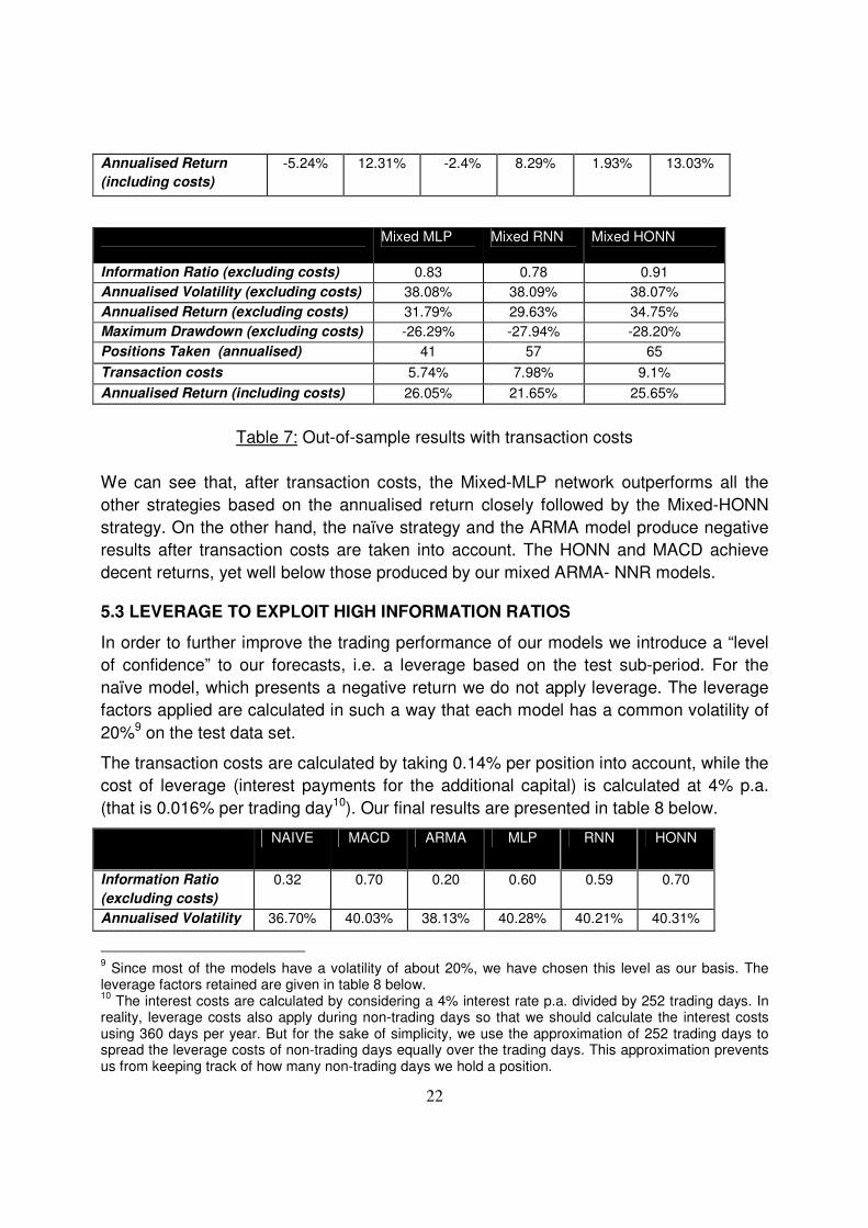
Annualised Return
(including costs)
-5.24% 12.31% -2.4% 8.29% 1.93% 13.03%
Mixed MLP Mixed RNN Mixed HONN
Information Ratio (excluding costs) 0.83 0.78 0.91
Annualised Volatility (excluding costs) 38.08% 38.09% 38.07%
Annualised Return (excluding costs) 31.79% 29.63% 34.75%
Maximum Drawdown (excluding costs) -26.29% -27.94% -28.20%
Positions Taken (annualised) 41 57 65
Transaction costs 5.74% 7.98% 9.1%
Annualised Return (including costs) 26.05% 21.65% 25.65%
Table 7: Out-of-sample results with transaction costs
We can see that, after transaction costs, the Mixed-MLP network outperforms all the
other strategies based on the annualised return closely followed by the Mixed-HONN
strategy. On the other hand, the naïve strategy and the ARMA model produce negative
results after transaction costs are taken into account. The HONN and MACD achieve
decent returns, yet well below those produced by our mixed ARMA- NNR models.
5.3 LEVERAGE TO EXPLOIT HIGH INFORMATION RATIOS
In order to further improve the trading performance of our models we introduce a “level
of confidence” to our forecasts, i.e. a leverage based on the test sub-period. For the
naïve model, which presents a negative return we do not apply leverage. The leverage
factors applied are calculated in such a way that each model has a common volatility of
20%9 on the test data set.
The transaction costs are calculated by taking 0.14% per position into account, while the
cost of leverage (interest payments for the additional capital) is calculated at 4% p.a.
(that is 0.016% per trading day10). Our final results are presented in table 8 below.
NAIVE MACD ARMA MLP RNN HONN
Information Ratio
(excluding costs)
0.32 0.70 0.20 0.60 0.59 0.70
Annualised Volatility 36.70% 40.03% 38.13% 40.28% 40.21% 40.31%
9 Since most of the models have a volatility of about 20%, we have chosen this level as our basis. The
leverage factors retained are given in table 8 below. 10
The interest costs are calculated by considering a 4% interest rate p.a. divided by 252 trading days. In reality, leverage costs also apply during non-trading days so that we should calculate the interest costs using 360 days per year. But for the sake of simplicity, we use the approximation of 252 trading days to spread the leverage costs of non-trading days equally over the trading days. This approximation prevents us from keeping track of how many non-trading days we hold a position.
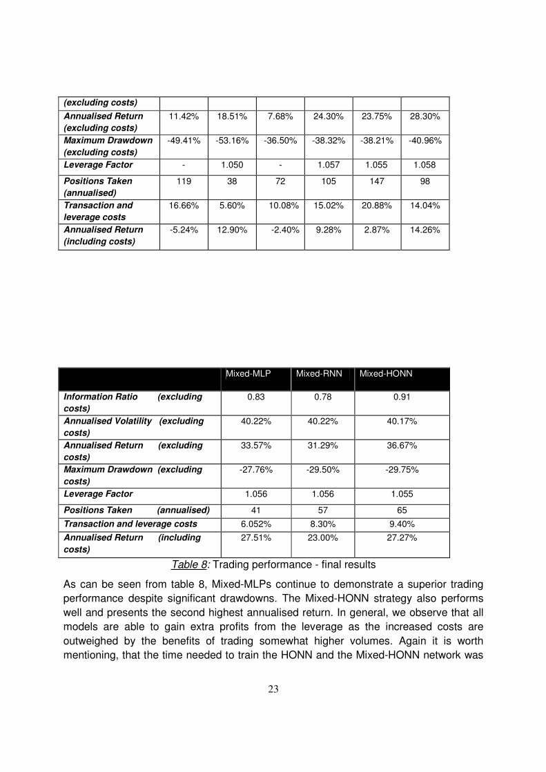
23
(excluding costs)
Annualised Return
(excluding costs)
11.42% 18.51% 7.68% 24.30% 23.75% 28.30%
Maximum Drawdown
(excluding costs)
-49.41% -53.16% -36.50% -38.32% -38.21% -40.96%
Leverage Factor - 1.050 - 1.057 1.055 1.058
Positions Taken
(annualised)
119 38 72 105 147 98
Transaction and
leverage costs
16.66% 5.60% 10.08% 15.02% 20.88% 14.04%
Annualised Return
(including costs)
-5.24% 12.90% -2.40% 9.28% 2.87% 14.26%
Mixed-MLP Mixed-RNN Mixed-HONN
Information Ratio (excluding
costs)
0.83 0.78 0.91
Annualised Volatility (excluding
costs)
40.22% 40.22% 40.17%
Annualised Return (excluding
costs)
33.57% 31.29% 36.67%
Maximum Drawdown (excluding
costs)
-27.76% -29.50% -29.75%
Leverage Factor 1.056 1.056 1.055
Positions Taken (annualised) 41 57 65
Transaction and leverage costs 6.052% 8.30% 9.40%
Annualised Return (including
costs)
27.51% 23.00% 27.27%
Table 8: Trading performance - final results
As can be seen from table 8, Mixed-MLPs continue to demonstrate a superior trading
performance despite significant drawdowns. The Mixed-HONN strategy also performs
well and presents the second highest annualised return. In general, we observe that all
models are able to gain extra profits from the leverage as the increased costs are
outweighed by the benefits of trading somewhat higher volumes. Again it is worth
mentioning, that the time needed to train the HONN and the Mixed-HONN network was

24
considerably shorter compared with that needed for the MLP, Mixed-MLP, RNN and the
Mixed-RNN networks.
6. CONCLUDING REMARKS
In this paper, we apply Multi-layer Percepton, Recurrent, Higher Order, Mixed-Multilayer
Percepton, Mixed-Recurrent and Mixed-Higher Order neural networks to a one-day-
ahead forecasting and trading task of the ASE 20 fixing series with only autoregressive
terms as inputs. We use a naïve strategy, a MACD and an ARMA model as
benchmarks. We develop these different prediction models over the period January
2001 - August 2007 and validate their out-of-sample trading efficiency over the following
period from September 2007 through December 2008.
The Mixed-HONNs demonstrates a higher trading performance in terms of annualised
return and information ratio before transaction costs and more elaborate trading
strategies are applied. When refined trading strategies are applied and transaction costs
are considered the Mixed-MLPs manage to outperform all other models achieving the
highest annualised return. The Mixed-HONNs and the Mixed-RNNs models perform
remarkably as well and seem to have an ability in providing good forecasts when
autoregressive series are only used as inputs.
It is also important to note that the Mixed-HONN network which presents a very close
second best performance needs less training time than Mixed-RNN and Mixed-MLP
network architectures, a much desirable feature in a real-life quantitative investment and
trading environment: in the circumstances, our results should go some way towards
convincing a growing number of quantitative fund managers to experiment beyond the
bounds of traditional statistical and neural network models. In particular, the strategy
consisting of modelling in a first stage the linear component of a financial time series

25
and then applying a neural network to learn its nonlinear elements appears quite
promising.
APPENDIX
A.1 ARMA Model
The output of the ARMA model used in this paper is presented below.
Dependent Variable: RETURNS
Method: Least Squares
Date: 03/17/09 Time: 22:18
Sample (adjusted): 8 1738
Included observations: 1731 after adjustments
Convergence achieved after 37 iterations
Backcast: 1 7
Variable Coefficient Std. Error t-Statistic Prob.
26
C 0.000290 0.000303 0.956602 0.3389
AR(1) 0.375505 0.052705 7.124626 0.0000
AR(3) -0.244662 0.024991 -9.789999 0.0000
AR(7) -0.678906 0.044902 -15.11958 0.0000
MA(1) -0.374290 0.053055 -7.054702 0.0000
MA(3) 0.269470 0.026409 10.20353 0.0000
MA(7) 0.677169 0.044295 15.28785 0.0000
R-squared 0.026582 Mean dependent var 0.000288
Adjusted R-squared 0.023194 S.D. dependent var 0.012549
S.E. of regression 0.012403 Akaike info criterion -5.937710
Sum squared resid 0.265213 Schwarz criterion -5.915645
Log likelihood 5146.088 F-statistic 7.846483
Durbin-Watson stat 1.856760 Prob(F-statistic) 0.000000
Inverted AR Roots .89-.44i .89+.44i .31-.92i .31+.92i
-.54+.70i -.54-.70i -.93
Inverted MA Roots .88-.45i .88+.45i .31-.92i .31+.92i
-.54+.70i -.54-.70i -.94
A.2 Performance Measures
The performance measures are calculated as follows:
Performance
Measure Description
Annualised Return ∑
=
=N
t
t
A RN
R1
1*252 [14]
with tR being the daily return
Cumulative Return ∑
=
=N
t
t
C RR1
[15]
Annualised
Volatility ( )∑
=
−−
=N
t
t
ARR
N 1
2*
1
1*252σ [16]
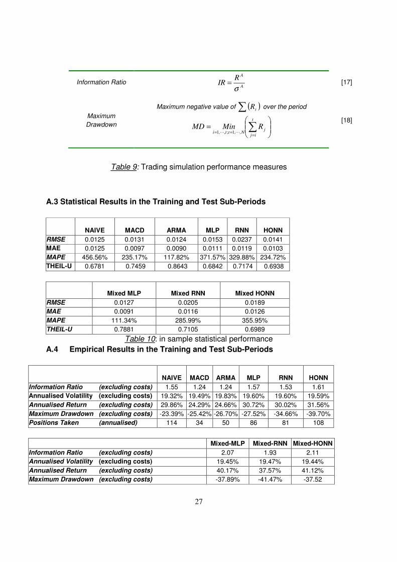
27
Information Ratio
A
ARIR
σ= [17]
Maximum
Drawdown
Maximum negative value of ( )∑ tR over the period
= ∑
===
t
ij
jNtti
RMinMD,,1;,,1 LL
[18]
Table 9: Trading simulation performance measures
A.3 Statistical Results in the Training and Test Sub-Periods
NAIVE MACD ARMA MLP RNN
HONN
RMSE 0.0125 0.0131 0.0124 0.0153 0.0237 0.0141
MAE 0.0125 0.0097 0.0090 0.0111 0.0119 0.0103
MAPE 456.56% 235.17% 117.82% 371.57% 329.88% 234.72%
THEIL-U 0.6781 0.7459 0.8643 0.6842 0.7174 0.6938
Mixed MLP Mixed RNN Mixed HONN
RMSE 0.0127 0.0205 0.0189
MAE 0.0091 0.0116 0.0126
MAPE 111.34% 285.99% 355.95%
THEIL-U 0.7881 0.7105 0.6989
Table 10: in sample statistical performance
A.4 Empirical Results in the Training and Test Sub-Periods
NAIVE MACD ARMA MLP RNN
HONN
Information Ratio (excluding costs) 1.55 1.24 1.24 1.57 1.53 1.61
Annualised Volatility (excluding costs) 19.32% 19.49% 19.83% 19.60% 19.60% 19.59%
Annualised Return (excluding costs) 29.86% 24.29% 24.66% 30.72% 30.02% 31.56%
Maximum Drawdown (excluding costs) -23.39% -25.42% -26.70% -27.52% -34.66% -39.70%
Positions Taken (annualised) 114 34 50 86 81 108
Mixed-MLP Mixed-RNN Mixed-HONN
Information Ratio (excluding costs) 2.07 1.93 2.11
Annualised Volatility (excluding costs) 19.45% 19.47% 19.44%
Annualised Return (excluding costs) 40.17% 37.57% 41.12%
Maximum Drawdown (excluding costs) -37.89% -41.47% -37.52
28
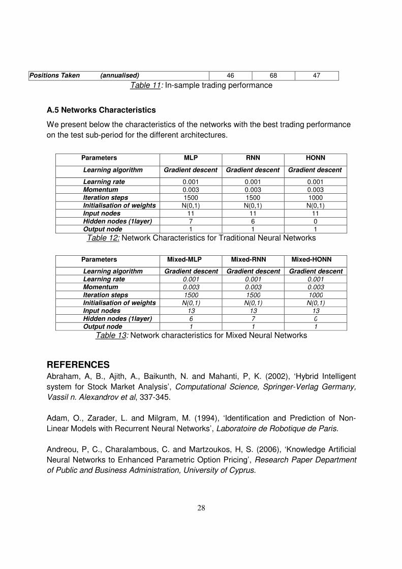
Positions Taken (annualised) 46 68 47
Table 11: In-sample trading performance
A.5 Networks Characteristics
We present below the characteristics of the networks with the best trading performance
on the test sub-period for the different architectures.
Table 12: Network Characteristics for Traditional Neural Networks
Table 13: Network characteristics for Mixed Neural Networks
REFERENCES Abraham, A, B., Ajith, A., Baikunth, N. and Mahanti, P, K. (2002), ‘Hybrid Intelligent
system for Stock Market Analysis’, Computational Science, Springer-Verlag Germany,
Vassil n. Alexandrov et al, 337-345.
Adam, O., Zarader, L. and Milgram, M. (1994), ‘Identification and Prediction of Non-
Linear Models with Recurrent Neural Networks’, Laboratoire de Robotique de Paris.
Andreou, P, C., Charalambous, C. and Martzoukos, H, S. (2006), ‘Knowledge Artificial
Neural Networks to Enhanced Parametric Option Pricing’, Research Paper Department
of Public and Business Administration, University of Cyprus.
Parameters MLP RNN HONN
Learning algorithm Gradient descent Gradient descent Gradient descent
Learning rate 0.001 0.001 0.001 Momentum 0.003 0.003 0.003
Iteration steps 1500 1500 1000 Initialisation of weights N(0,1) N(0,1) N(0,1) Input nodes 11 11 11
Hidden nodes (1layer) 7 6 0 Output node 1 1 1
Parameters Mixed-MLP Mixed-RNN Mixed-HONN
Learning algorithm Gradient descent Gradient descent Gradient descent
Learning rate 0.001 0.001 0.001 Momentum 0.003 0.003 0.003
Iteration steps 1500 1500 1000 Initialisation of weights N(0,1) N(0,1) N(0,1) Input nodes 13 13 13
Hidden nodes (1layer) 6 7 0 Output node 1 1 1
29
Bishop, C., (1994) ‘Mixture Density Networks’. Neural Computing Research Group
Report: NCRG/94/004, 1–25.
Box, G., Jenkins, G. and Gregory, G. (1994), Time Series Analysis: Forecasting and
Control, Prentice-Hall, New Jersey.
Brown, G., Wyatt, J., Harris, R., and Yao, X. (2005), ‘Diversity Creation Methods: A
Survey and Categorization’, Information Fusion, 6, 5–20.
Clemen, R. (1989), ‘Combining Forecasts: A Review and Annotated Bibliography’,
International Journal of Forecasting, 5, 559–583.
Connor, J. and Atlas, L. (1993), ‘Recurrent Neural Networks and Time Series
Prediction’, Proceedings of the International Joint Conference on Neural Networks, 301-
306.
Dunis, C. and Huang, X. (2002), ‘Forecasting and Trading Currency Volatility: An
Application of Recurrent Neural Regression and Model Combination’, Journal of
Forecasting, 21, 5, 317-354.
Dunis, C., Laws, J. and Evans B. (2006a), ‘Trading Futures Spreads: An Application of
Correlation and Threshold Filters’, Applied Financial Economics, 16, 1-12.
Dunis, C., Laws, J. and Evans B. (2006b), ‘Modelling and Trading the Gasoline Crack
Spread: A Non-Linear Story’, Derivatives Use, Trading and Regulation, 12, 126-145.
Dunis, C., Laws, j and Karathanasopoulos A. (2010a), ‘Modelling and Trading the
Greek Stock Market with Hybrid ARMA-Neural Network Models’, CIBEF Working
Papers. Available at www.cibef.com
Dunis, C., Laws, J. and Sermpinis, G. (2008a), ‘Higher Order and Recurrent Neural
Architectures for Trading the EUR/USD Exchange Rate’, CIBEF Working Papers.
Available at www.cibef.com
Dunis, C., Laws, J. and Sermpinis, G. (2008b), ‘Modelling and Trading the EUR/USD
Exchange Rate at the ECB Fixing’, CIBEF Working Papers. Available at www.cibef.com
Dunis, C. and Chen, Y. (2005), ‘Alternative Volatility Models for Risk Management and
Trading: Application to the EUR/USD and USD/JPY Rates’, Derivative Use, Trading &
Regulation, 11, 2, 126-156

30
Elman, J. L. (1990), ‘Finding Structure in Time’, Cognitive Science, 14, 179-211.
Fatima, S. and Hussain, G., (2008) ‘Statistical Models of KSE100 Index Using Hybrid
Financial Systems’, Neurocomputing, 7, 2742-2746.
Fulcher, J., Zhang, M. and Xu, S. (2006), ‘The Application of Higher-Order Neural
Networks to Financial Time Series’, Artificial Neural Networks in Finance and
Manufacturing, Hershey, PA: Idea Group, London.
Ghiassi, M., Saidane, H. and Zimbra D. K. (2005), ‘A Dynamic Artificial Neural Network
Model for Forecasting Series Events’, International Journal of Forecasting, 21, 341-362.
Giles, L. and Maxwell, T. (1987) ‘Learning, Invariance and Generalization in Higher
Order Neural Networks’, Applied Optics, 26, 4972-4978.
Greg, T. and Hu, S. (1999), ‘Forecasting GDP Growth Using Artificial Neural Network’,
Working Paper, Bank of Canada, 99-3.
Hansen, J. and Nelson, R., (2003) ‘Time-Series Analysis with Neural Networks and
ARIMA-Neural Network Hybrids’, Journal of Experimental and Theoretical Artificial
Intelligence, 15 (3), 315–330.
Hibbert, H., Pedreira, C. and Souza, R., (2000) ‘Combining Neural Networks and ARIMA
Models for Hourly Temperature Forecast’, Proceedings of International Conference on
Neural Networks (IJCNN 2000), 414–419.
Hibon, M. and Evgeniou. T., (2005) ‘To Combine or not to Combine: Selecting among
Forecasts and their Combinations’, International Journal of Forecasting, 22, 15-24.
Kaastra, I. and Boyd, M. (1996), ‘Designing a Neural Network for Forecasting Financial
and Economic Time Series’, Neurocomputing, 10, 215-236.
Kamijo, K. and Tanigawa,T. (1990), ‘Stock Price Pattern Recognition: A Recurrent
Neural Network Approach’, In Proceedings of the International Joint Conference on
Neural Networks, 1215-1221.
Karayiannis, N. and Venetsanopoulos, A. (1994), ‘On the Training and Performance of
High-Order Neural Networks’, Mathematical Biosciences, 129, 143-168.

31
Knowles, A., Hussein, A., Deredy, W., Lisboa, P. and Dunis, C. L. (2009), ‘Higher-Order
Neural Networks with Bayesian Confidence Measure for Prediction of EUR/USD
Exchange Rate’, Artificial Higher Order Neural networks for Economic and Business, 1,
48-59, CIBEF Working Papers. Available at www.cibef.com.
Kosmatopoulos, E., Polycarpou, M., Christodoulou, M. and Ioannou, P. (1995), ‘High-
Order Neural Network Structures for Identification of Dynamical Systems’, IEEE
Transactions on Neural Networks, 6, 422-431.
Lindemann, A., Dunis, C. and Lisboa P. (2004), ‘Level Estimation, Classification and
Probability Distribution Architectures for Trading the EUR/USD Exchange Rate’. Neural
Network Computing & Applications, 14, 3, 256-271.
Makridakis, S., Anderson A., Carbone, R., Fildes, R., Hibdon, M., Lewandowski, R.,
Newton, J., Parzen, E. and Winkler, R., (1982) ‘The Accuracy of Extrapolation (Time
Series) Methods: Results of a Forecasting Competition’, Journal of Forecasting, 1, 111–
153.
Makridakis, S., (1989) ‘Why Combining Works?’, International Journal of Forecasting, 5,
601–603.
Newbold, P. and Granger, C. W. J., (1974) ‘Experience with Forecasting Univariate Time
Series and the Combination of Forecasts (with discussion)’, Journal of Statistics, 137,
131–164.
Palm, F.C. and Zellner, A., (1992), ‘To Combine or not to Combine? Issues of
Combining Forecasts’, Journal of Forecasting, 11, 687–701.
Pindyck, R. and Rubinfeld, D. (1998), Econometric Models and Economic Forecasts, 4th
edition, McGraw-Hill, New York.
Psaltis, D., Park, C. and Hong, J. (1988), ‘Higher Order Associative Memories and their
Optical Implementations’, Neural Networks, 1, 149-163.
Redding, N., Kowalczyk, A. and Downs, T. (1993), ‘Constructive Higher-Order Network
Algorithm that is Polynomial Time’, Neural Networks, 6, 997-1010.
Shapiro, A. F. (2000), ‘A Hitchhiker’s Guide to the Techniques of Adaptive Nonlinear
Models’, Insurance, Mathematics and Economics, 26, 119-132.
32
Tenti, P. (1996), ‘Forecasting Foreign Exchange Rates Using Recurrent Neural
Networks’, Applied Artificial Intelligence, 10, 567-581.
Terui, N. and van Dijk, H. (2002), ‘Combined Forecasts from Linear and Nonlinear Time
Series Models’, International Journal of Forecasting, 18, 421–438.
Theil, H. (1996), ‘Applied Economic Forecasting, North-Holland, Amsterdam,
Netherlands.
Tseng, F.M., Yu, H.C. and Tzeng, G.H., (2002) ‘Combining Neural Network Model with
Seasonal Time Series ARIMA Model’, Technological Forecasting and Social Change,
69, 71–87.
Wang, Y. F., (2007) ‘Nonlinear Neural Network Forecasting Model for Stock Index
Option Price: Hybrid GJR-GARCH Approach’, Expert Systems with Applications, 475-
484.
Zhang, M., Xu, S., X. and Fulcher, J. (2002), ‘Neuron-Adaptive Higher Order Neural-
Network Models for Automated Financial Data Modelling’, IEEE Transactions on Neural
Networks, 13, 1, 188-204.
Zhang, G.P., (2003) ‘Time Series Forecasting Using a Hybrid ARIMA and Neural
Network Model’, Neurocomputing, 50, 159–175.
Zhang, G. P., and Qi, M., (2005) ‘Neural Network Forecasting for Seasonal and Trend
Time Series’, European Journal of Operational Research, 160 (2), 501–514.
Recommended