Cesar Augusto Conopoima Perez
Mortar Finite Element Method for cell response to applied electric field
Dissertacao apresentada ao Programade Pos-graduacao em ModelagemComputacional, da Universidade Federalde Juiz de Fora como requisito parcial aobtencao do grau de Mestre em ModelagemComputacional.
Orientador: Prof. D.Sc. Bernardo Martins Rocha
Coorientador: Prof. D.Sc. Rodrigo Weber Dos Santos
Coorientador: Prof. D.Sc. Iury Higor Aguiar Da Igreja
Juiz de Fora
2017
Ficha catalográfica elaborada através do programa de geração automática da Biblioteca Universitária da UFJF,
com os dados fornecidos pelo(a) autor(a)
Conopoima Pérez, Cesar Augusto. Mortar Finite Element Method for cell response to applied electricfield / Cesar Augusto Conopoima Pérez. -- 2017. 69 p. : il.
Orientador: Bernardo Martins Rocha Coorientadores: Rodrigo Weber dos Santos, Iury Higor Aguiar daIgreja Dissertação (mestrado acadêmico) - Universidade Federal deJuiz de Fora, ICE/Engenharia. Programa de Pós-Graduação emModelagem Computacional, 2017.
1. Mortar Finite Element Method. 2. Lagrange multiplier. 3.Passive and active response of the cell. 4. Applied electric field. I.Martins Rocha, Bernardo, orient. II. Weber dos Santos, Rodrigo,coorient. III. Aguiar da Igreja, Iury Higor, coorient. IV. Título.

To the nature.

ACKNOWLEDGEMENTS
First of all I would like to thank to the Pos-graduate Program in Computational
Modelling of the Federal University of Juiz de Fora, for choosing me as international
student in the program, I also thank to all the professors which I meet and have
fruitful discussions during the master courses, specially I would like to thank professor
Bernardo Martins Rocha by allowing me to work over his nicely constructed FEM library
(cardiax). I also thank him for his guidance and patience, every meeting was a profitable
time that allow this work to be finished; to professor Iury da Igreja by the hours of
informal discussion about The Finite Elements Method, they were certainly very useful
to conclude this work; to professor Rodrigo Weber dos Santos also by his guidance and
for the informal talks about everything, in particular about electrophysiology, his insights
and knowledge truly enriched this work.
I am also very thankful to all the friends in the laboratory, some for making the coffee
break an enjoyable time, and others for the interesting chatting about they research
works. I am grateful to all the Brazilians, specially to the Mineiros, that I encounter
and lived during this time in Brazil, they make me feel authentically welcome in their
country, all the personal and professional growth I experience in the past year was only
possible thanks to them. Finally I am very grateful to Marissa Scardua by her patient
and help in difficult times, her unmeasurable kindness and love inspire me every day.
To CAPES for the financial support during the development of this work and during
the complete master course.
ABSTRACT
The response of passive and active biological cell to applied electric field is investigated
with a Mortar Finite Element Method MFEM. Cells response is a process with two
different time scales, one in microseconds for the cell polarization and the other in
milliseconds for the active response of the cell due to the complex dynamics of the ion-
channel current on the cell membrane. The mathematical model to describe the dynamics
of the cell response is based on the conservation law of electric current in a conductive
medium. By introducing an additional variable known as Lagrange multiplier defined on
the cell interface, the boundary value problem associated to the conservation of electric
current is decoupled from the initial value problem associated to the passive and active
response of the cell. The proposed method allows to solve electric potential distribution in
arbitrary cell geometry and arrangements. In order to validate the presented methodology,
the h-convergence order of the MFEM is numerically investigated. The numerical and
exact solutions describing cell polarization are also compared. Finally, to demonstrate
the effectiveness of the method, the active response to an applied electric field in cells
clusters and cells with arbitrary geometry are investigated.
Key-words: Mortar Finite Element Method. Lagrange Multiplier. Passive and active
response of the cell. Applied electric field.
RESUMO
A resposta passiva e ativa de uma celula biologica a um campo eletrico e estudada
aplicando um Metodo de Elementos Finitos Mortar MEFM. A resposta de uma celula
e um processo com duas escalas temporais, o primeiro na escala de microsegundos para a
polarizacao da celula e o segundo na escala de milisegundos para a resposta ativa devido
a dinamica complexa das correntes nos canais ionicos da membrana celular. O modelo
matematico para descrever a dinamica da resposta celular e baseado na lei de conservacaao
de corrente eletrica em um meio condutor. Introduzindo uma variavel adicional conhecida
como multiplicador de Lagrange definido na interface da celula, o problema de valor de
fronteira associado a conservacao de corrente eletrica e desacoplado do problema de valor
inicial associado a responta passiva e ativa da celula. O metodo proposto permite resolver
o problema da distribuicao de potencial eletrico em um arranjo geometrico arbitrario de
celulas. Com o objetivo de validar a metodologia apresentada, a convergencia espacial
do metodo e numericamente investigada e a solucao aproxima e exata que descreve a
polarizacao de uma celula, sao comparadas. Finalmente, para demonstrar a efetividade
do metodo, a resposta ativa a um campo eletrico aplicado num arranjo de celulas de
geometria arbitraria e investigada.
Palavras-Chaves: Metodo de Elementos Finitos Mortar. Multiplicador de Lagrange.
Resposta ativa e passiva da celula. Campo eletrico aplicado.
CONTENTS
1 Introduction . . . . . . . . . . . . . . . . . . . . . . . . . . . . . . . . . . . . . . . . . . . . . . . . . . . . . . . . . 14
1.1 Interface problems by FEM . . . . . . . . . . . . . . . . . . . . . . . . . . . . . . . . . . . . . . . 15
1.2 Objectives . . . . . . . . . . . . . . . . . . . . . . . . . . . . . . . . . . . . . . . . . . . . . . . . . . . . . . . . 17
1.3 Structure of the work . . . . . . . . . . . . . . . . . . . . . . . . . . . . . . . . . . . . . . . . . . . . . 17
2 Biological response of cell to applied electrical field . . . . . . . . . . . . . . . . . . . 18
2.1 Mathematical models . . . . . . . . . . . . . . . . . . . . . . . . . . . . . . . . . . . . . . . . . . . . . . 18
2.1.1 Model for electric response of a cell. . . . . . . . . . . . . . . . . . . . . . . . . . . . 20
2.1.2 The Hodgkin-Huxley model . . . . . . . . . . . . . . . . . . . . . . . . . . . . . . . . . . . . 22
3 The Mortar Finite Element Method . . . . . . . . . . . . . . . . . . . . . . . . . . . . . . . . . . 26
3.1 Preliminaries . . . . . . . . . . . . . . . . . . . . . . . . . . . . . . . . . . . . . . . . . . . . . . . . . . . . . . 26
3.1.1 Linear variational formulation problems of one field. . . . . . . . . . . . 27
3.1.2 Linear mixed variational formulation problems . . . . . . . . . . . . . . . . . 28
3.2 The model problem . . . . . . . . . . . . . . . . . . . . . . . . . . . . . . . . . . . . . . . . . . . . . . . 31
3.2.1 Existence and uniqueness of the saddle point problem . . . . . . . . . . 34
3.3 Finite element discretization . . . . . . . . . . . . . . . . . . . . . . . . . . . . . . . . . . . . . . 35
3.3.1 The mortar finite element discretization . . . . . . . . . . . . . . . . . . . . . . . 37
3.3.2 Error estimate . . . . . . . . . . . . . . . . . . . . . . . . . . . . . . . . . . . . . . . . . . . . . . . . 39
3.4 Time discretization for the transmembrane current . . . . . . . . . . . . . . . . 40
4 Computational aspects of the Saddle Point Problem . . . . . . . . . . . . . . . . . . 42
4.1 Structure of the indefinte linear system . . . . . . . . . . . . . . . . . . . . . . . . . . . . 42
4.2 Numerical methods to solve saddle point problems . . . . . . . . . . . . . . . . 44
4.2.1 Schur Complement . . . . . . . . . . . . . . . . . . . . . . . . . . . . . . . . . . . . . . . . . . . . 44
4.2.2 Penalty method . . . . . . . . . . . . . . . . . . . . . . . . . . . . . . . . . . . . . . . . . . . . . . . 46
4.2.3 Krylov space method . . . . . . . . . . . . . . . . . . . . . . . . . . . . . . . . . . . . . . . . . . 47
5 Results . . . . . . . . . . . . . . . . . . . . . . . . . . . . . . . . . . . . . . . . . . . . . . . . . . . . . . . . . . . . . . 48
5.1 h-convergence of the method . . . . . . . . . . . . . . . . . . . . . . . . . . . . . . . . . . . . . . 48
5.2 Exact and numerical solution of the cell interface problem . . . . . . . . . 51

5.3 Complex dynamics of the ion current and action potential . . . . . . . . . 56
6 Conclusions . . . . . . . . . . . . . . . . . . . . . . . . . . . . . . . . . . . . . . . . . . . . . . . . . . . . . . . . . . 62
6.1 Future works . . . . . . . . . . . . . . . . . . . . . . . . . . . . . . . . . . . . . . . . . . . . . . . . . . . . . . 63
REFERENCES . . . . . . . . . . . . . . . . . . . . . . . . . . . . . . . . . . . . . . . . . . . . . . . . . . . . . . . . . 64
LIST OF FIGURES
2.1 A circular cell in a conductive medium . . . . . . . . . . . . . . . . . . . . . . 20
2.2 Polar reference system used in the exact solution. . . . . . . . . . . . . . . . . 22
2.3 Transmembrane potential following the action potential described the
Hodgkin-Huxley model for an applied current Im = 5[µA · cm−2] and
activation variables of the ions channels. . . . . . . . . . . . . . . . . . . . 25
3.1 A circular cell in a conductive medium . . . . . . . . . . . . . . . . . . . . . . 31
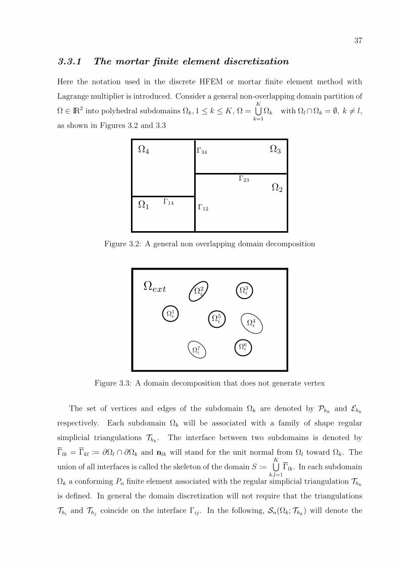
3.2 A general non overlapping domain decomposition . . . . . . . . . . . . . . . . 37
3.3 A domain decomposition that does not generate vertex . . . . . . . . . . . . . 37
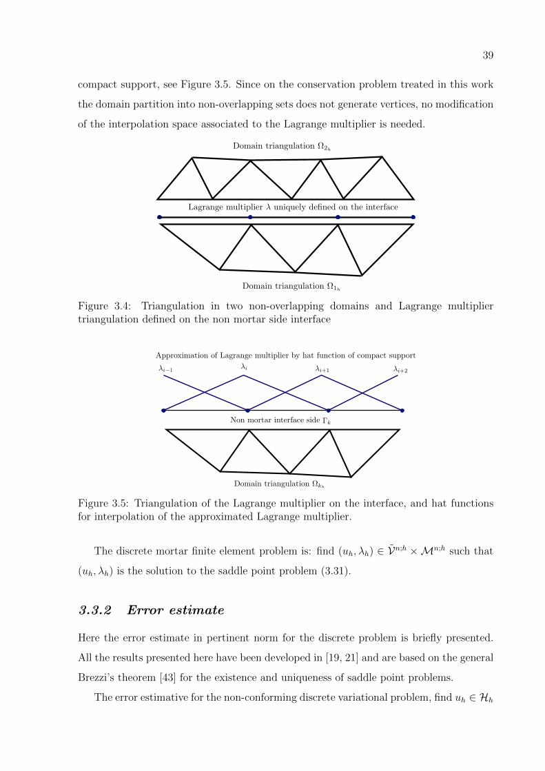
3.4 Triangulation in two non-overlapping domains and Lagrange multiplier
triangulation defined on the non mortar side interface . . . . . . . . . . . . 39
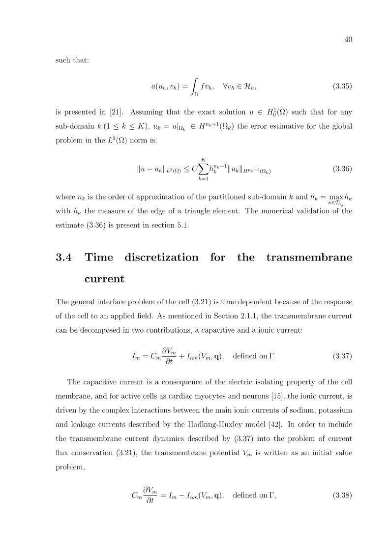
3.5 Triangulation of the Lagrange multiplier on the interface, and hat functions
for interpolation of the approximated Lagrange multiplier. . . . . . . . . . 39
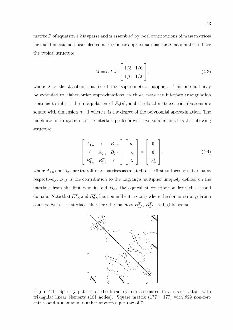
4.1 Sparsity pattern of the linear system associated to a discretization with
triangular linear elements (161 nodes). Square matrix (177 × 177) with
929 non-zero entries and a maximum number of entries per row of 7. . . . . 43
5.1 Computational domain and numerical solution of the second order interface
problem. . . . . . . . . . . . . . . . . . . . . . . . . . . . . . . . . . . . . . 49
5.2 Domain discretization by triangular linear finite elements, matching
discretization left and non-matching discretization at right. . . . . . . . . . 49
5.3 h-convergence study for the primal variable and the Lagrange multiplier for a
triangular discretization with matching elements. . . . . . . . . . . . . . . 50
5.4 At left the circular cell and the reference system used in the exact solution, at
top right the electric potential inside and outside the cell as function of the
radius r for a fixed angle θ = 0; on the bottom right the transmembranic
potential Vm = ui − ue defined on the cell interface as a function of the
angular position θ ∈ [0, 360]. . . . . . . . . . . . . . . . . . . . . . . . . . . 51
5.5 Transmembrane current in time. . . . . . . . . . . . . . . . . . . . . . . . . . . 52
5.6 A circular cell in a conductive medium . . . . . . . . . . . . . . . . . . . . . . 53
5.7 Cell domain discretization with triangular elements. . . . . . . . . . . . . . . . 53
5.8 Reference system of the circular cell to plot the numerical and exact solution. 54
5.9 Electric potential in function of the angle evaluated at the membrane for the
passive response of the cell with matching grids. Exact solution is plotted
as continuous functions, and the numerical results are plotted as the dotted
lines. . . . . . . . . . . . . . . . . . . . . . . . . . . . . . . . . . . . . . . . 54
5.10 Left: steady state iso-potential contour around the cell. Right: the domain
discretization by triangular elements used to solve the polarization process
in the isolated cell. The distance between electrodes is 0.01[cm], the applied
electric field is E = 5[V · cm−1] and cell diameter is dc = 15[µm], the intra
and extracellular conductivities are κi = 5[mS·cm−1] and κe = 20[mS·cm−1]
respectively. . . . . . . . . . . . . . . . . . . . . . . . . . . . . . . . . . . . 55
5.11 Left the iso-potential contour in a cluster of cells after 1.0[µs] of simulation.
Right: the matching domain discretization used to solve the polarization
process in the cell cluster. The distance between electrodes is 0.02[cm], the
applied electric field is E = 5[V · cm−1] and cells diameter are dc = 15[µm],
the intra and extracellular conductivities are the same as for isolated cell
case. . . . . . . . . . . . . . . . . . . . . . . . . . . . . . . . . . . . . . . . 55
5.12 Circular biological cell with a transmembranic potential Vm = −65[mV] at rest
(t = 0). . . . . . . . . . . . . . . . . . . . . . . . . . . . . . . . . . . . . . . 56
5.13 Distribution of the electric potential of the active response of a circular cell. . 57
5.14 Active response of the cell to an applied electrical field of E = 10[V · cm−1].
Each curve correspond with the time curse of electric potential in a fixed
angular position (θ) at fixed radius r = dc2
. . . . . . . . . . . . . . . . . . . 58
5.15 Response of the cell to an applied electrical field of E = 6[V · cm−1]. Each
curve correspond with the time curse of electric potential in a fixed angular
position on the cell interface. . . . . . . . . . . . . . . . . . . . . . . . . . . 59
5.16 Distribution of the electric potential of the active response of cell cluster. At
top left the used non-conforming domains discretization is showed. The
distance between the cells at right and left is 24 [µm]. . . . . . . . . . . . . 60

5.17 Active response of a cell cluster to an applied electrical field of E = 20[V·cm−1].
Each curve correspond with the time course of electric potential in a fixed
angular position on every cell interface. . . . . . . . . . . . . . . . . . . . . 61

LIST OF TABLES
5.1 h−convergence order for the approximation of uh and λh obtained by the
MFEM for matching triangular elements. . . . . . . . . . . . . . . . . . . . 50
5.2 h−convergence order for the approximation of uh and λh obtained by the
MFEM for non-matching triangular elements. . . . . . . . . . . . . . . . . 50
14
1 Introduction
The response of a single cell and cluster of cells to external applied electrical field
is important for the understanding of techniques such as cell electroporation [1, 2],
which is the transient permeabilization of the plasma membrane by means of short
and intense electric pulse. This technique has broad application in the biological and
medical community for instance for the local treatment of cancer. Since the cells cytosol
becomes accessible to the external medium, DNA and molecules transference into the
cell is possible, direct drug supply is also possible without compromising cell function
[1, 2]. Moreover, it is not clear if cell electroporation does play an important role in
cardiac defibrillation, therefore this is also a relevant topic in the research field of cardiac
electrophysiology [3, 4, 5]. Properly studying extracellular potential distribution in cluster
of cells of arbitrary geometry is important to understand the influence of applied electrical
field in neurons activity [6].
Particular solutions to describe the passive response of cells to applied field are
available for isolated cells of simple circular and ellipsoidal geometry [7, 8]. Although
exact solutions for spherical cells in non uniform electric field exists [9, 10], a general tool
to numerically investigate cells electroporation and extracellular potential distribution
is of interest. In this sense, the numerical study of the passive and active response of
isolated cells to external field has been made in [11, 12]. Furthermore the influence
of cells arrangement, orientation and cells packing in the presence of external electrical
applied field has also been investigated in [13, 14, 11, 6].
The response of biological cells to applied electrical field is a two stage process [7, 11]:
the first stage takes place at the time scale of microseconds, where the capacitive current
is dominant and the cell behaves like a dipole; in the second stage actual physiological
changes due to the complex dynamics of ion currents on the cell membrane, which is
triggered if the transmembrane current on the first stage is sufficiently high to unchain
an action potential on the cell [15]. Moreover the active response of the cell will also be
influenced by the distribution and packing of the cells [14, 6]. Because of the complex
interactions in cells arrangements, possible irregular cells geometries and the lack of exact
solutions in those cases, the study of the distribution of electric potential and of the

15
action potential in non-idealized systems of multiple cells can only be studied by numerical
methods.
In the context of numerical methods, in particular the Finite Element Methods (FEM),
simulations of cells electroporation in tumours [16], non regular cell geometry [12] and
spherical cell arrangements [13] have been investigated. In [14, 6] a Hybrid Finite Element
Method (HFEM) is used to investigate the passive and active cell response to external
applied electrical fields. With this method the boundary value problem of electric flux
conservation and the initial value problem of active cell response are decoupled and
solved in alternate form in each time step. The HFEM is based on the hypothesis
that cell membrane is a zero thickness domain i.e, an interface that separates two non
overlapping domains [11], the intra and the extracellular domains. The membrane imposes
an interface condition inside the domain which must be properly treated. In the context of
finite element methods, one possible approach is to formulate separated problems in each
domain and impose compatibility of the solution on the interface via Lagrange multipliers.
1.1 Interface problems by FEM
Proper treatment of interface conditions in finite element methods [17, 18], requires the
imposition of continuity of the solution on the interface through Lagrange multipliers, as
proposed by Raviart-Thomas in the known primal hybrid formulation [19]. This approach
allows to have non-conforming domain discretizations with optimal convergence order for
both the primal and Lagrange multiplier variables [20, 21].
In order to satisfy the compatibility condition between spaces (LBB inf-sup condition)
in the primal hybrid formulation, the Lagrange multiplier must be properly defined. The
formal treatment and analysis of this method are defined in the literature as Mortar Finite
Element Method [20, 21, 22, 23]; and has the main advantage of allowing to solve interface
problems with non-matching domain triangulations. The linear system associated with
the discrete version of this formulation has a saddle point problem structure and in general
is difficult to solve numerically [24]. This difficulty can be circumvent by including Galekin
Least Square (GLS) stabilizations terms [25, 26, 27], or by approximating the Lagrange
multiplier using a dual multiplier space. In the second case static condensation is possible
for the Lagrange multiplier and effective multigrid solvers can be used [28, 22, 23].
16
Another form to satisfy the interface condition is to impose continuity of the primal
variable and of the flux on the interface in a weak form. This gives rise to a three field
domain decomposition method as proposed in [29]. Optimal order approximations for
all the fields [26, 29, 30] is proved with proper stabilizations terms [25]. This method
includes two Lagrange multiplier spaces, one associated with the flux on the interface and
other associated to the trace of the function at the interface. The indefinite linear system
obtained from the finite element discretization, is sparser and bigger than the obtained by
the primal hybrid formulation due to the inclusion of two additional field to the original
problem, however its advantage is the possibility of using different approximations spaces
for the flux and the trace of the primal variable on the interface.
In the context of mixed finite elements [31, 32], Raviart-Thomas spaces are required
[31] and continuity of the solution on the interface may be imposed by a constrained
function space [32] or, in a weak form, through Lagrange multipliers. In the latter case
super optimal order approximations of the primal variable may be achieved by a post-
processing technique [33].
Imposing continuity of the solution on the interface through auxiliary Lagrange
multipliers spaces requires the solution of an indefinite linear system. For the primal
hybrid formulation this system is poorly conditioned demanding particular solution
techniques [24, 28]. Another possibility to impose continuity of the solution through
the interface is by penalization methods [34] or Nitsche type methods [35], where the
continuity of the solution is imposed by coupled weighted terms of the primal variable
defined in the interface. This family of methods generates a global system less sparse than
those arising in standard conforming FEM [36]. These techniques were demonstrated to be
particularly interesting to solve highly convective problems due to the inner stabilization
mechanism [37].
To relax the coupling introduced by the interface terms a hybridization technique can
be applied as proposed in [38] and analyzed in [39][40], which is particularly interesting
when discontinuous finite elements are used in all the computational domain. In these
cases a positive definite global system is assembled from local contributions by static
condensation and direct linear solvers can be effectively used.
17
1.2 Objectives
In this work the active and passive response of isolated cells to applied field is investigated
with a Mortar Finite Element Method MFEM. The main objective of this work is to apply
the MFEM to handle the solution discontinuity due to the response of the cell interface by
using non conforming domains discretizations and conforming Galerkin C0 discretizations
on the rest of the domain. It is also the objective of this work to present the conditions
for the existence and uniqueness to the solution of the variational formulation, the space
compatibility condition and error estimate in natural norm confirmed through numerical
examples. Finally, the effectiveness of the method will be demonstrated by solving the
interface problem in an isolated cell and cluster of cells with non-matching discretizations.
1.3 Structure of the work
This work is structured as follows: in Chapter 2 the conservation law of electric flux
in biological conductive mediums is presented, the interface conditions between domains
of different conductivities is also introduced and an exact solution to the conservation
problem for an isolated circular cell in a conductive medium is presented. In Chapter
3 a preliminary section is dedicated to the basic theory of function spaces, then the
model problem is introduced and the primal hybrid variational formulation is deduced;
the existence and uniqueness of the formulation is proved and the mortar finite element
discretization is presented. In Chapter 4 the computational aspects of the saddle point
problem are outlined. In Chapter 5 the h-convergence of the proposed method are
determined and numerical results of the passive and active response of the cell are
presented. Finally, in Chapter 6 the final remarks are made and the proposal for futures
works are discussed.
18
2 Biological response of cell to
applied electrical field
Understanding cell polarization under the action of external electrical field has wide
applications in techniques as electrochemotherapy, permeabilization of cell membrane by
electroporation, neuronal stimulation, cardiac pacing and cardiac defibrillation [1, 2, 6, 5].
By means of numerical simulations it is possible to understand the phenomenology of
electric potential distribution in complex cell geometries and arrangements. From the
conservation law of electric current in a conductive medium in the presence of a cell or a
group of cells, it is possible to deduce a mathematical model based on partial differential
equations (PDE) that describes the distribution of electric potential in the medium and
in the biological cell.
2.1 Mathematical models
The electric field in a biological tissue resulting from the application of a direct current
can be considered quasi-stationary [41], this means that its distribution is described by
equations of the steady electric current in a volume conductor. The relation of electric
current to voltage and resistance is described by Ohm’s law. The electric current density
J[A · cm−3] is defined by the point form of the Ohm’s law J = κ · E, where E[V · cm−1]
is the electric vector field,
E = −∇u, (2.1)
where u[V] is the scalar electric potential. In Ohm’s law, κ[S · cm−1] is the electric
conductivity of the biological tissue and in the most generalized case it is a second order
tensor. When conductivity is expressed in terms of a orthogonal coordinated system
(x, y, z) and both the electric field and current density are related to the same coordinate
system, κ is diagonal with entries of the conductivity values defined on the principal
directions.
By continuity of current density, the Kirchoff’s law can be written in differential form
as div(J) = ρs, where ρs[A ·cm−3] is an applied source current. Now by Ohm’s law applied
19
to a electric field, we can write Kirchoff’s law in terms of the electric potential u as,
−div(κ∇u) = ρs, (2.2)
which is known as the Poisson’s equation that describe the electric potential distribution
in a resistive biological tissue with an applied source current. The boundary value
problem (2.2) requires additional conditions in order to be well posed. Dirichlet boundary
conditions can be defined on the domain’s boundary to denote an applied voltage, or
Neumann boundary conditions when a current source is applied on some portion of the
boundary.
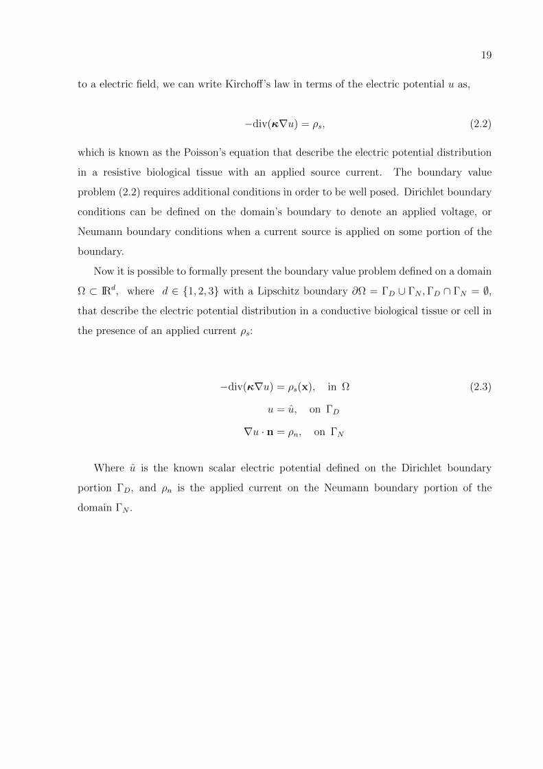
Now it is possible to formally present the boundary value problem defined on a domain
Ω ⊂ IRd, where d ∈ 1, 2, 3 with a Lipschitz boundary ∂Ω = ΓD ∪ ΓN ,ΓD ∩ ΓN = ∅,
that describe the electric potential distribution in a conductive biological tissue or cell in
the presence of an applied current ρs:
−div(κ∇u) = ρs(x), in Ω (2.3)
u = u, on ΓD
∇u · n = ρn, on ΓN
Where u is the known scalar electric potential defined on the Dirichlet boundary
portion ΓD, and ρn is the applied current on the Neumann boundary portion of the
domain ΓN .
20
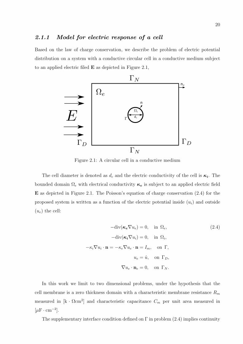
2.1.1 Model for electric response of a cell
Based on the law of charge conservation, we describe the problem of electric potential
distribution on a system with a conductive circular cell in a conductive medium subject
to an applied electric filed E as depicted in Figure 2.1,
Figure 2.1: A circular cell in a conductive medium
The cell diameter is denoted as dc and the electric conductivity of the cell is κi. The
bounded domain Ωe with electrical conductivity κe is subject to an applied electric field
E as depicted in Figure 2.1. The Poisson’s equation of charge conservation (2.4) for the
proposed system is written as a function of the electric potential inside (ui) and outside
(ue) the cell:
−div(κe∇ue) = 0, in Ωe, (2.4)
−div(κi∇ui) = 0, in Ωi,
−κi∇ui · n = −κe∇ue · n = Im, on Γ,
ue = u, on ΓD,
∇ue · ne = 0, on ΓN .
In this work we limit to two dimensional problems, under the hypothesis that the
cell membrane is a zero thickness domain with a characteristic membrane resistance Rm
measured in [k · Ωcm2] and characteristic capacitance Cm per unit area measured in
[µF · cm−2].
The supplementary interface condition defined on Γ in problem (2.4) implies continuity
21
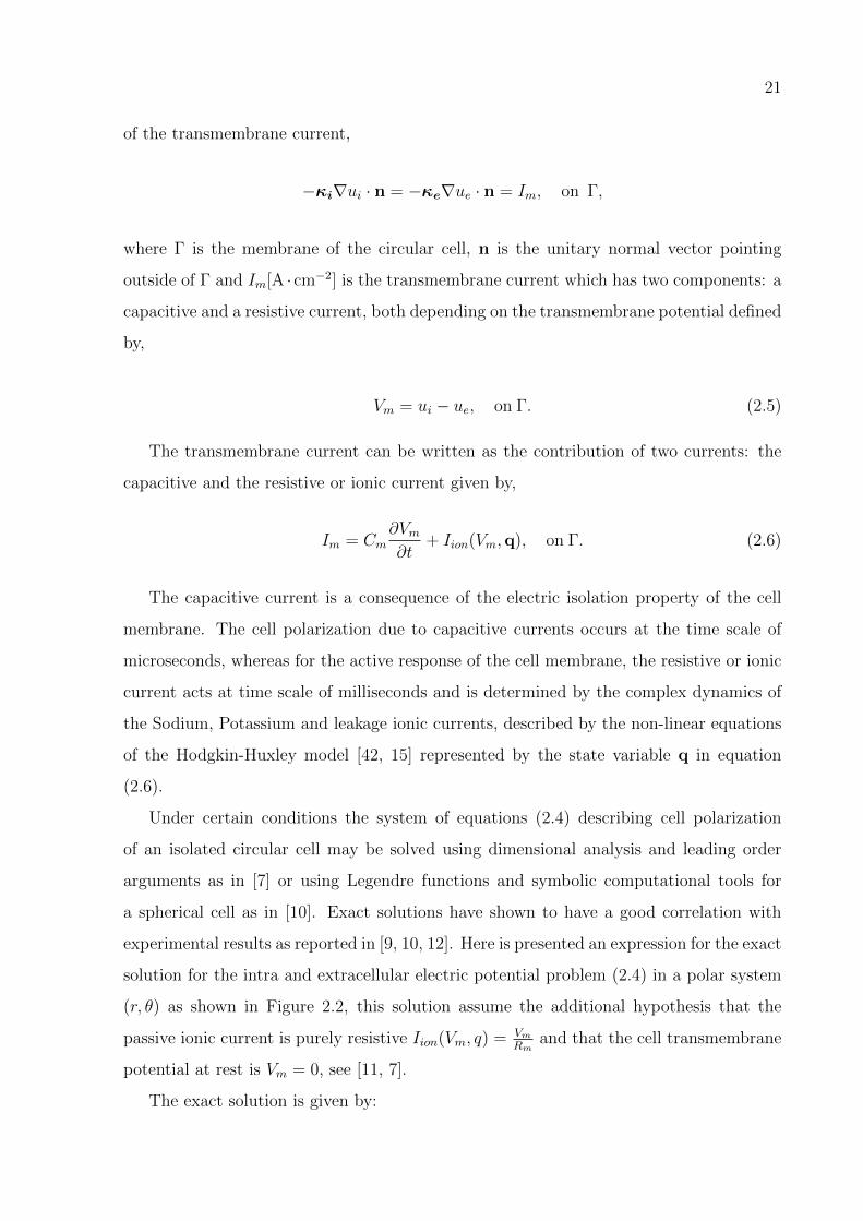
of the transmembrane current,
−κi∇ui · n = −κe∇ue · n = Im, on Γ,
where Γ is the membrane of the circular cell, n is the unitary normal vector pointing
outside of Γ and Im[A · cm−2] is the transmembrane current which has two components: a
capacitive and a resistive current, both depending on the transmembrane potential defined
by,
Vm = ui − ue, on Γ. (2.5)
The transmembrane current can be written as the contribution of two currents: the
capacitive and the resistive or ionic current given by,
Im = Cm∂Vm∂t
+ Iion(Vm,q), on Γ. (2.6)
The capacitive current is a consequence of the electric isolation property of the cell
membrane. The cell polarization due to capacitive currents occurs at the time scale of
microseconds, whereas for the active response of the cell membrane, the resistive or ionic
current acts at time scale of milliseconds and is determined by the complex dynamics of
the Sodium, Potassium and leakage ionic currents, described by the non-linear equations
of the Hodgkin-Huxley model [42, 15] represented by the state variable q in equation
(2.6).
Under certain conditions the system of equations (2.4) describing cell polarization
of an isolated circular cell may be solved using dimensional analysis and leading order
arguments as in [7] or using Legendre functions and symbolic computational tools for
a spherical cell as in [10]. Exact solutions have shown to have a good correlation with
experimental results as reported in [9, 10, 12]. Here is presented an expression for the exact
solution for the intra and extracellular electric potential problem (2.4) in a polar system
(r, θ) as shown in Figure 2.2, this solution assume the additional hypothesis that the
passive ionic current is purely resistive Iion(Vm, q) = VmRm
and that the cell transmembrane
potential at rest is Vm = 0, see [11, 7].
The exact solution is given by:
22
Figure 2.2: Polar reference system used in the exact solution.
ui(r, θ, t) = −a(t) · Ercos(θ), r <dc2
(2.7)
ue(r, θ, t) = −Ercos(θ)− b(t) · E d2c
4rcos(θ), r >
dc2
Vm(θ, t) = Edccos(θ)(1− e−t/τip)(1− ε).
Where
a(t) =2κe
κi + κe
e−t/τip + ε(1− e−t/τip)
b(t) = 1− 2κi
κi + κe
e−t/τip + ε(1− e−t/τip)
τip =
1
CmRm
+2κiκe
Cmdc(κi + κe)
ε =
τipCmRm
The passive response of the cell take place at the characteristic time scale τip of
microseconds. In Chapter 5 the phenomenology of cell polarization described by this
solution is presented. Even though exact solutions as (2.7) exists to describe the passive
response of the cell in simple geometries, it is a limited tool to solve more general cases.
In the next chapter, the variational formulation of the conservation problem (2.4) is
presented, this approach will be the ground base to find approximated solutions of general
cases problems.
2.1.2 The Hodgkin-Huxley model
In 1952 Alan Lloyd Hodgkin and Andrew Fielding Huxley determined in a quantitative
form [42] the relation between the main ionic currents going through the cell membrane
23
and the transmembrane potential describing the propagation of action potential on the
giant squid axon. The main ionic currents described by the Hodgkin-Huxley HH model
are the sodium, potassium and leakage current INa, IK , Il respectively. The HH model
idealize the flux of electric current trough the cell membrane as a closed circuit between
the intra and extracellular domain, the transmembrane potential in the absence of an
applied current is given by the balance between the capacitive and ionic currents:
−CmdVmdt
= INa + IK + Il, (2.8)
where Cm is the electric capacitance of the lipid bilayer of the cell membrane measured
in [µF · cm2]. Each ionic currents can be expressed as function of the ionic conductivity
of the sodium, potassium and others (gNa, gK , gl) as:
INa = gNa(Vm − ENa), (2.9)
IK = gK(Vm − EK), (2.10)
Il = gl(Vm − El), (2.11)
where ENa, EK and El are the potential of equilibrium for each species. The great
contribution of the HH model was the description of the ionic conductivities (gNa, gK , gl)
during the action potential in function of the transmembrane potential Vm. The ionic
conductivity of sodium and potassium are given by:
gNa = gNam3h, (2.12)
dm
dt= αm(1−m)− βmm, (2.13)
dh
dt= αh(1− h)− βhh, (2.14)
gK = gKn4, (2.15)
dn
dt= αn(1− n)− βnn, (2.16)
where gNa and gK are the maximal conductance value measured in [S·cm−2] of the sodium
and potassium, m, h and n are dimensionless variables ∈ [0, 1] related to the activation
of the sodium and potassium ion channels; αm, αh, βm, βh, αn and βn are functions of Vm
24
and represent the activation and deactivation rate of the associated ion channels:
αm =0.1(Vm + 25)
eVm+25
10 − 1, (2.17)
βm = 4eVm18 , (2.18)
αh = 0.07eVm20 , (2.19)
βh =1
eVm+30
10 + 1, (2.20)
αn =0.01(Vm + 10)
eVm+10
10 − 1, (2.21)
βn = 0.125eVm80 . (2.22)
The electric conductivity associated to the leakage ionic current gl is simply determined
as gl = gl the maximal conductance value. The final expression of the HH model is then:
−CmdVmdt
= gNam3h(Vm − ENa) + gKn
4(Vm − EK) + gl(Vm − El)− Im, (2.23)
where Im is the transmembrane current, in this work the transmembrane current on the
active response of the cell, will be considered to be the applied current due to an electric
field that will trigger or not the action potential on the cell membrane. For a detailed
description over the experimental setting and the physiological considerations see [15, 42].
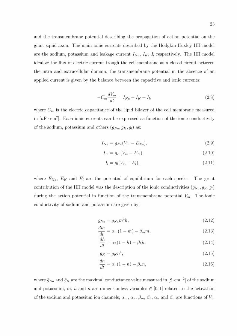
In Figure 2.3 the transmembrane potential Vm describing the action potential typical
of the giant squid axon described by the HH model is plotted, the activations variables of
the model m,n and h are also shown. The parameters to reproduce the action potential
are: gNa = 120[mS · cm−2], gK = 36[mS · cm−2], gl = 0.3[mS · cm−2], ENa = 115[mV],
EK = −12[mV], El = 10.6[mV], Cm = 1[µF · cm−2], Im = 5[µA · cm−2] and (m,n, h) =
(0.1, 0.33, 0.6) at t = 0. The transmembrane potential Vm is considered to be a deviation
from the equilibrium state of the cell Vm = V − Veq where the typical value of Veq for the
experimental setting of the HH model is Veq = −65[mV], see [15, 42].
25
Figure 2.3: Transmembrane potential following the action potential described theHodgkin-Huxley model for an applied current Im = 5[µA · cm−2] and activation variablesof the ions channels.
26
3 The Mortar Finite Element
Method
In this chapter the notation used in this work is introduced and some aspects of the
functional space where the mortar finite element method is based are also presented.
The variational formulation of the second order interface problem of the cell response to
applied electric field is introduced and, the conditions for the existence and uniqueness of
the solution as proposed by Raviart-Thomas [19] are presented, finally the a priori error
estimative of the discrete problem is briefly presented.
3.1 Preliminaries
The adopted notation in this work is the following, u, v and φ denote scalar fields; u,
v, φ denote vectorial fields. We consider a bounded domain Ω ⊂ IR2, with a Lipschitz
boundary ∂Ω and bounded real valued functions f ∈ L2(Ω), where L2(Ω) denotes the
space of functions square integrable in Ω.
For a given m ≥ 0 ∈ N, we denote the Hilbert space Hm(Ω) of order m on Ω containing
functions v ∈ L2(Ω) such that the m−th derivative in the sense of distributions are defined
in L2(Ω), that is:
Hm =v ∈ L2(Ω);Dαv ∈ L2(Ω), |α| ≤ m
, where, (3.1)
Dα(·) =∂α(·)∂α1x1 ∂
α2x2
, |α| = α1 + α2, (3.2)
and α is a vector of non-negative integer entries. The inner product defined in Hm(Ω)
and its associated norm are given by:
(v, w)m :=∑|α|<m
∫Ω
DαvDαwdx, ‖v‖2m = (v, v)m. (3.3)
The space L2(Ω) is then H0(Ω) and in this work the associated norm ‖v‖L2(Ω) will
simply be denoted by ‖v‖0.
27
The particular Hilbert spaces of interest in the present work are: L2(Ω), H1(Ω), H10 (Ω)
and H12 (Ω). If the boundary of the bounded domain Ω, denoted by ∂Ω is a Lipschitz
continuous domain, there exists a linear and continuous operator γ0 : H1(Ω) → L2(∂Ω)
called the trace operator; γ0 applied to v ∈ H1(Ω) is simply the restriction of v to ∂Ω,
denoted as v|∂Ω. The application of the trace operator γ0 to H1(Ω), γ0(H1(Ω)) belongs
to a family of normed Hilbert spaces Hs(∂Ω) with s ∈ IR, in particular:
γ0(H1(Ω)) := H12 (∂Ω),
with the associated norm,
‖γ0v‖H 12 (∂Ω)
:= infv∈H1(Ω)
‖v‖H1(Ω).
The dual space of H12 (∂Ω) is denoted by H−
12 (∂Ω), and the duality relation between
these two spaces is given by,
< ·, · >∂Ω:=
∫∂Ω
µvds.
3.1.1 Linear variational formulation problems of one field
The linear variational problem of a single field can be represented in an abstract form as,
given f ∈ U ′ find u ∈ U such that:
a(u, v) = f(v), ∀v ∈ U , (3.4)
where U is a Hilbert space, U ′ the associated dual space and a(·, ·) : U × U → IR is a
bilinear form. For cases where the bilinear form is symmetric and positive definite, this
problem is equivalent to the following minimization problem: find u ∈ U such that
J(u) ≤ J(v), ∀v ∈ U ,
with
J(v) =1
2a(v, v)− f(v), ∀v ∈ U .
The analysis of the existence and uniqueness to the solution of problem (3.4) is ensured
by the Lax-Milgram theorem.
28
Theorem 3.1. (The Lax-Milgram theorem). If U is a Hilbert space, f : U → IR a
continuous linear functional and a(·, ·) : U × U → IR is a bilinear form such that:
1. It is continuous: there exists a constant 0 < M <∞ such that
|a(u, v)| ≤M‖u‖U‖v‖U ∀u, v ∈ U (3.5)
2. It is U-Elliptic: there exists a constant α > 0 such that
|a(u, v)| ≥ α‖u‖‖v‖ ∀u, v ∈ U (3.6)
then the variational problem (3.4) has a unique solution.
3.1.2 Linear mixed variational formulation problems
Linear variational problems on the presence of internal constrains handled via Lagrange
multipliers [19], leads to variational problems of two fields commonly denoted as mixed
problems [32]; postulated here in abstract form as, given f ∈ U ′ and g ∈ M′, find
(u, λ) ∈ U ×M such that:
a(u, v) + b(v, λ) = f(v), ∀v ∈ U , (3.7)
b(u, µ) = g(µ), ∀µ ∈M,
where U and M are Hilbert spaces, a : U × U → IR, b : U ×M → IR are continuous
bilinear forms and f : U → IR and g : M → IR are continuous linear functionals. The
bilinear forms a(·, ·) and b(·, ·) defines the following norms:
‖a‖ = supu,v∈U
a(u, v)
‖u‖U‖v‖U,
‖b‖ = supv∈U ,µ∈M
b(v, µ)
‖v‖U‖µ‖M,
and also defines the following linear continuous operators A : U → U ′, B : U → M′ and
Bt :M→ U ′ given by:
< Au, v >U ′×U= a(u, v), ∀u, v ∈ U ,
29
< Bv, µ >M′×M=< v,BTµ >U×U ′ , ∀u ∈ U , µ ∈M.
When the bilinear form a(·, ·) is symmetric and elliptic in the space:
K(0) =v ∈ U ; b(v, µ) = 0, ∀µ ∈M
, (3.8)
it is possible to associated problem (3.7) with the following minimization problem, find
u ∈ K(g) such that:
J(v) =1
2a(v, v)− f(v), in K(g),
with
K(g) =v ∈ U ; b(v, µ) = g(µ), ∀µ ∈M
.
Using the technique of Lagrange multiplier, the problem (3.7) can be transformed in the
following saddle point problem, find (u, λ) ∈ U ×M such that:
L(u, µ) ≤ L(u, λ) ≤ L(v, λ), ∀v ∈ U , ∀µ ∈M (3.9)
where L(v, µ) is the Langrangian functional,
L(v, λ) = J(v) + (Bv − g, λ) (3.10)
with λ the Lagrange multiplier.
The conditions for the existence and uniqueness of the problem (3.7) is presented here
through the auxiliary problem: find u ∈ K(g) such that
a(u, v) = f(v), ∀v ∈ ker(B) = K(0). (3.11)
Note that if (u, λ) ∈ U ×M solves problem (3.7), then u ∈ K(g) also solves problem
(3.11). Now, the conditions to satisfy the inverse relation, this is, given u ∈ K(g) solving
problem (3.11) there exist a pair (u, λ) ∈ U ×M solving problem (3.7) are given in the
following theorem.
Theorem 3.2. (Brezzi theorem). If U and M are Hilbert spaces, f : U → IR and
g : M → IR are continuous linear functionals and a(·, ·) : U × U → IR and b(·, ·) :
U ×M→ IR are bilinear forms which satisfied:
30
1. Continuity: there exists two constants 0 < M1, M2 <∞ such that
|a(u, v)| ≤M1‖u‖U‖v‖U ∀u, v ∈ U
|b(u, λ)| ≤M2‖u‖U‖λ‖M ∀u ∈ U ∀λ ∈M
2. K-Coercivity of a: exists two constants α1 > 0 and α2 > 0 such that
supv∈K
|a(u, v)|‖v‖U
≥ α1‖u‖U ∀u ∈ K
supu∈K
|a(u, v)|‖u‖U
≥ α2‖v‖U ∀v ∈ K
where,
K(0) =u ∈ U ; b(u, µ) = 0 ∀µ ∈M
3. LBB-condition: exists a constant β > 0 such that
supv∈U
|b(v, λ)|‖v‖U
≥ β‖µ‖M ∀µ ∈M
Then the problem (3.7) has a unique solution.
After this short presentation of the basic theory of variational problems, the variational
formulation and finite element discretization for the model problem of the response of a
cell to an applied electric field, is introduced and briefly analysed.
31
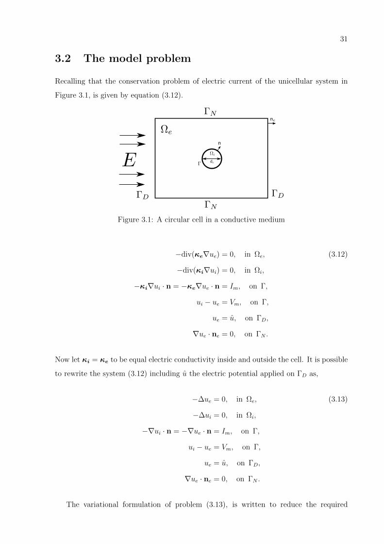
3.2 The model problem
Recalling that the conservation problem of electric current of the unicellular system in
Figure 3.1, is given by equation (3.12).
Figure 3.1: A circular cell in a conductive medium
−div(κe∇ue) = 0, in Ωe, (3.12)
−div(κi∇ui) = 0, in Ωi,
−κi∇ui · n = −κe∇ue · n = Im, on Γ,
ui − ue = Vm, on Γ,
ue = u, on ΓD,
∇ue · ne = 0, on ΓN .
Now let κi = κe to be equal electric conductivity inside and outside the cell. It is possible
to rewrite the system (3.12) including u the electric potential applied on ΓD as,
−∆ue = 0, in Ωe, (3.13)
−∆ui = 0, in Ωi,
−∇ui · n = −∇ue · n = Im, on Γ,
ui − ue = Vm, on Γ,
ue = u, on ΓD,
∇ue · ne = 0, on ΓN .
The variational formulation of problem (3.13), is written to reduce the required
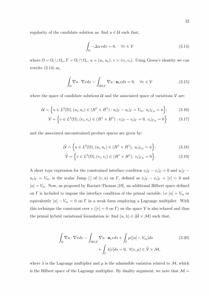
32
regularity of the candidate solution as: find u ∈ U such that,
∫Ω
−∆uvdx = 0, ∀v ∈ V (3.14)
where Ω = Ωi ∪ Ωe, Γ = Ωi ∩ Ωe, u = (ui, ue), v = (vi, ve). Using Green’s identity we can
rewrite (3.14) as,
∫Ω
∇u · ∇vdx−∫∂Ω\Γ∇u · nevds = 0, ∀v ∈ V (3.15)
where the space of candidate solutions U and the associated space of variations V are:
U =u ∈ L2(Ω), (ui, ue) ∈ (H1 ×H1) : ui|Γ − ue|Γ = Vm, ue|ΓD
= u
; (3.16)
V =v ∈ L2(Ω), (vi, ve) ∈ (H1 ×H1) : vi|Γ − ve|Γ = 0, ve|ΓD
= 0
(3.17)
and the associated unconstrained product spaces are given by:
U =u ∈ L2(Ω), (ui, ue) ∈ (H1 ×H1), ue|ΓD
= u
; (3.18)
V =v ∈ L2(Ω), (vi, ve) ∈ (H1 ×H1), ve|ΓD
= 0. (3.19)
A short type expression for the constrained interface condition vi|Γ − ve|Γ = 0 and ui|Γ −
ue|Γ = Vm, is the scalar Jump [·] of (v, u) on Γ, defined as vi|Γ − ve|Γ = [v] = 0 and
[u] = Vm. Now, as proposed by Raviart-Thomas [19], an additional Hilbert space defined
on Γ is included to impose the interface condition of the primal variable, i.e [u] = Vm or
equivalently [u] − Vm = 0 on Γ in a weak form employing a Lagrange multiplier. With
this technique the constraint over v ([v] = 0 on Γ) on the space V is also relaxed and thus
the primal hybrid variational formulation is: find (u, λ) ∈ (U ×M) such that,
∫Ω
∇u · ∇vdx−∫∂Ω\Γ∇u · nevds+
∫Γ
µ([u]− Vm)ds (3.20)
+
∫Γ
λ[v]ds = 0, ∀(v, µ) ∈ V ×M,
where λ is the Lagrange multiplier and µ is the admissible variation related toM, which
is the Hilbert space of the Lagrange multiplier. By duality argument, we note thatM =
33
H−12 (Γ), which is the dual space of H
12 (Γ) and therefore µ ∈ H− 1
2 (Γ). The variational
formulation (3.20) can be derived from a minimization problem under a relaxed manifold
and is known as a saddle point problem, see [19, 32]. By the natural Neumann boundary
condition in (3.13)(f) ∇u ·ne = 0 on ΓN , the second term of the formulation is neglected,
and then the saddle point problem is: find (u, λ) ∈ (U ,M) such that
a(u, v) + b(v, λ) = 0, ∀v ∈ V (3.21)
b(u, µ) = g(µ), ∀µ ∈M
with a(u, v) =∫
Ω∇u · ∇vdx, b(v, µ) =
∫Γµ[v]ds and g(µ) =
∫ΓµVmds. A different way to
write a variational formulation of the original interface problem (3.13) is now presented.
The objective is to find the relation between the interface condition of flux conservation
on (3.13)(c) and how this is satisfied by the formulation (3.21). Assuming that we chose
two functions (vi, ve) ∈ V with compact support on (Ωi,Ωe) respectively, multiplying by
the two first equations in (3.13) and using the Green’s integration identity, the following
variational problem is obtained: find (ui, ue) ∈ U such that
∫Ωe
∇ue · ∇vedx−∫∂Ω\Γ∇ue · neveds+
∫Γ
∇ue · nveds = 0, ∀v ∈ V , (3.22)∫Ωi
∇ui · ∇vidx−∫
Γ
∇ui · nvids = 0, ∀v ∈ V ,
where (ui, ue) must satisfy the interface conditions [u] = Vm on Γ and −∇ui · n =
−∇ue · n = Im, on Γ with n = ni = −ne the normal unitary vector pointing outward
Γ. Considering that the flux interface condition is explicitly written in (3.22) and that
the Neumann boundary condition of 3.13(f) on ΓN is included on the formulation, it is
possible to rewrite (3.22) as:
∫Ωe
∇ue · ∇vedx−∫
Γ
Imveds = 0, ∀v ∈ V , (3.23)∫Ωi
∇ui · ∇vidx+
∫Γ
Imvids = 0, ∀v ∈ V ,
As postulated (vi, ve) have compact support on (Ωi,Ωe), therefore it is possible to
define a unique function u = (ui, ue) and v = (vi, ve) such that by adding the two first
34
equations on (3.23) we have the equivalent variational formulation: find u ∈ U such that
∫Ω
∇u · ∇vdx+
∫Γ
Im[v]ds = 0, ∀v ∈ V , (3.24)
Choosing Im := λ i.e the transmembrane current to be the Lagrange multiplier defined on
Γ and by including the interface condition [u] = Vm on Γ in a weak form with the function
of admissible variations of λ ∈ M, this is µ ∈ M, equation (3.24) recovers the primal
hybrid variational formulation (3.21): find (u, λ) ∈ (U ,M) such that
∫Ω
∇u · ∇vdx+
∫Γ
λ[v]ds = 0, ∀v ∈ V , (3.25)∫Γ
µ[u]ds =
∫Γ
µVmds, ∀µ ∈M,
In this process the following relation can be identified, Im ≡ λ ≡ −∇ui ·n ≡ −∇ue ·n.
3.2.1 Existence and uniqueness of the saddle point problem
The essential points to proof the existence and uniqueness of the solution to the saddle
point problem (3.25) are: continuity, coercivity and suitable inf-sup condition. The proof
for the general interface problem (3.25) is fully detailed in [23], however here for the sake
of presentation the proof will be presented as in [19, 21], where the interface condition
over Γ of the primal variable is simply: [u] = Vm = 0 and the general Dirichlet condition
ue|ΓD= u is replaced by the homogeneous condition in all the boundary, that is ue|∂Ω = 0
with ∂Ω = ΓD ∪ ΓN .
The Hilbert space H10 (Ω) can be defined as a subspace of V containing the functions
satisfying the matching condition over the interface in a weak form, that is,
(v, µ)→ b(v, µ) =
∫Γ
[v]µds = 0, ∀µ ∈M. (3.26)
Using the Hahn-Banach theorem as presented by Raviart and Thomas in [19], it can
be proved that a Hilbert space H with the same characteristics of H10 (Ω) can be defined
as:
H :=v ∈ V , b(v, µ) = 0, ∀µ ∈M(Γ)
.
35
Now let (u, λ) ∈ (V ×M) be the solution of the following saddle point problem
a(u, v) + b(v, λ) = 0, ∀v ∈ V (3.27)
b(u, µ) = 0, ∀µ ∈M.
Because of the characterization of the space H, it is possible to say that u ∈ H solves
problem (3.27). Now by letting v ∈ H the variational formulation (3.27) can be rewritten
as: find u ∈ H such that,
a(u, v) = 0, ∀v ∈ H. (3.28)
Note that problem (3.28) is the classic 2nd order elliptic problem with homogeneous
Dirichlet boundary condition, and as a consequence u ∈ H is the unique solution of both
problems (3.28) and (3.27), see [19].
Now remain the issue of the uniqueness of the Lagrange multiplier, to prove it consider
u ∈ H solving problem (3.28) and that the following continuous linear functional on V is
satisfied in H:
L→ −a(u, v), (3.29)
then from equation (3.27)(a) it is possible to write,
b(v, λ) = −a(u, v), ∀v ∈ V . (3.30)
As postulated −a(u, v) is satisfied in H, therefore −a(u, v) = 0. By the Lemma 1 in
Raviart and Thomas [19] page 393 there exist a unique λ ∈M satisfying equation (3.30).
With this result, the existence and uniqueness of the solution (u, λ) ∈ (V × M) of the
saddle point problem (3.27) is proved.
3.3 Finite element discretization
The discrete method to approximate the saddle point problem of the cell interface problem
is based on problem (3.27) for proper conforming spaces Vh ⊂ V and Mh ⊂ M. Then,
36
the discrete problem is: find a pair (uh, λh) ∈ (Vh ×Mh) such that:
a(uh, vh) + b(vh, λh) = 0, ∀v ∈ Vh (3.31)
b(uh, µh) = 0, ∀µ ∈Mh.
An important difference between the discrete and continuous form of the saddle point
problem is worth to mention here. For this, we introduce the discrete space Hh,
Hh =vh ∈ Vh; b(vh, µh) = 0, ∀µh ∈Mh
. (3.32)
The space Hh may be considered an approximation of H, however Hh is not in general a
conforming space of H. The discrete version of the elliptic problem (3.28) is: find uh ∈ Hh
such that
a(uh, vh) = 0, ∀vh ∈ Hh, (3.33)
Since in general Hh 6⊂ H, the problem (3.33) is a non-conforming method to
approximate problem (3.28). If (uh, λh) ∈ Vh × Mh is a solution of problem (3.31),
uh ∈ Hh is a solution of problem (3.33) (see [19]). Moreover the following result is
obtained:
Theorem 3.3. If ‖vh‖2h = a(vh, vh) is a norm over Hh, then:
1. Problem (3.33) has a unique solution uh ∈ Hh;
2. Problem (3.31) has a unique solution (uh, λh) ∈ Vh×Mh if and only if the following
compatibility condition holds
µh ∈Mh; ∀vh ∈ Vh, b(vh, µh) = 0
=
0
(3.34)
The proof for the existence and uniqueness of the discrete problem can be found in
[19].
37
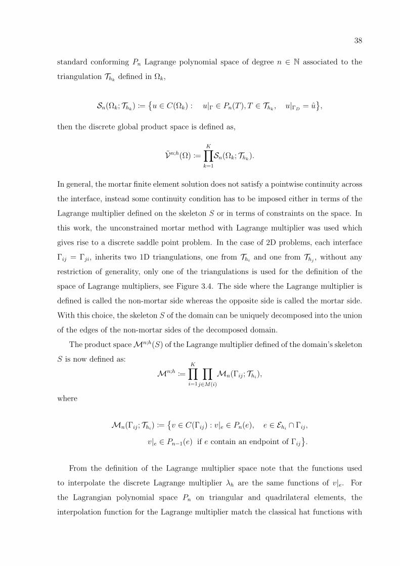
3.3.1 The mortar finite element discretization
Here the notation used in the discrete HFEM or mortar finite element method with
Lagrange multiplier is introduced. Consider a general non-overlapping domain partition of
Ω ∈ IR2 into polyhedral subdomains Ωk, 1 ≤ k ≤ K, Ω =K⋃k=1
Ωk with Ωl∩Ωk = ∅, k 6= l,
as shown in Figures 3.2 and 3.3
Figure 3.2: A general non overlapping domain decomposition
Figure 3.3: A domain decomposition that does not generate vertex
The set of vertices and edges of the subdomain Ωk are denoted by Phk and Ehkrespectively. Each subdomain Ωk will be associated with a family of shape regular
simplicial triangulations Thk . The interface between two subdomains is denoted by
Γlk = Γkl := ∂Ωl ∩ ∂Ωk and nlk will stand for the unit normal from Ωl toward Ωk. The
union of all interfaces is called the skeleton of the domain S :=K⋃
k,l=1
Γlk. In each subdomain
Ωk a conforming Pn finite element associated with the regular simplicial triangulation Thkis defined. In general the domain discretization will not require that the triangulations
Thi and Thj coincide on the interface Γij. In the following, Sn(Ωk; Thk) will denote the
38
standard conforming Pn Lagrange polynomial space of degree n ∈ N associated to the
triangulation Thk defined in Ωk,
Sn(Ωk; Thk) :=u ∈ C(Ωk) : u|Γ ∈ Pn(T ), T ∈ Thk , u|ΓD
= u,
then the discrete global product space is defined as,
Vn;h(Ω) :=K∏k=1
Sn(Ωk; Thk).
In general, the mortar finite element solution does not satisfy a pointwise continuity across
the interface, instead some continuity condition has to be imposed either in terms of the
Lagrange multiplier defined on the skeleton S or in terms of constraints on the space. In
this work, the unconstrained mortar method with Lagrange multiplier was used which
gives rise to a discrete saddle point problem. In the case of 2D problems, each interface
Γij = Γji, inherits two 1D triangulations, one from Thi and one from Thj , without any
restriction of generality, only one of the triangulations is used for the definition of the
space of Lagrange multipliers, see Figure 3.4. The side where the Lagrange multiplier is
defined is called the non-mortar side whereas the opposite side is called the mortar side.
With this choice, the skeleton S of the domain can be uniquely decomposed into the union
of the edges of the non-mortar sides of the decomposed domain.
The product spaceMn;h(S) of the Lagrange multiplier defined of the domain’s skeleton
S is now defined as:
Mn;h :=K∏i=1
∏j∈M(i)
Mn(Γij; Thi),
where
Mn(Γij; Thi) :=v ∈ C(Γij) : v|e ∈ Pn(e), e ∈ Ehi ∩ Γij,
v|e ∈ Pn−1(e) if e contain an endpoint of Γij.
From the definition of the Lagrange multiplier space note that the functions used
to interpolate the discrete Lagrange multiplier λh are the same functions of v|e. For
the Lagrangian polynomial space Pn on triangular and quadrilateral elements, the
interpolation function for the Lagrange multiplier match the classical hat functions with
39
compact support, see Figure 3.5. Since on the conservation problem treated in this work
the domain partition into non-overlapping sets does not generate vertices, no modification
of the interpolation space associated to the Lagrange multiplier is needed.
Figure 3.4: Triangulation in two non-overlapping domains and Lagrange multipliertriangulation defined on the non mortar side interface
Figure 3.5: Triangulation of the Lagrange multiplier on the interface, and hat functionsfor interpolation of the approximated Lagrange multiplier.
The discrete mortar finite element problem is: find (uh, λh) ∈ Vn;h ×Mn;h such that
(uh, λh) is the solution to the saddle point problem (3.31).
3.3.2 Error estimate
Here the error estimate in pertinent norm for the discrete problem is briefly presented.
All the results presented here have been developed in [19, 21] and are based on the general
Brezzi’s theorem [43] for the existence and uniqueness of saddle point problems.
The error estimative for the non-conforming discrete variational problem, find uh ∈ Hh
40
such that:
a(uh, vh) =
∫Ω
fvh, ∀vh ∈ Hh, (3.35)
is presented in [21]. Assuming that the exact solution u ∈ H10 (Ω) such that for any
sub-domain k (1 ≤ k ≤ K), uk = u|Ωk∈ Hnk+1(Ωk) the error estimative for the global
problem in the L2(Ω) norm is:
‖u− uh‖L2(Ω) ≤ C
K∑k=1
hnk+1k ‖uk‖Hpk+1(Ωk) (3.36)
where nk is the order of approximation of the partitioned sub-domain k and hk = maxκ∈Thk
hκ
with hκ the measure of the edge of a triangle element. The numerical validation of the
estimate (3.36) is present in section 5.1.
3.4 Time discretization for the transmembrane
current
The general interface problem of the cell (3.21) is time dependent because of the response
of the cell to an applied field. As mentioned in Section 2.1.1, the transmembrane current
can be decomposed in two contributions, a capacitive and a ionic current:
Im = Cm∂Vm∂t
+ Iion(Vm,q), defined on Γ. (3.37)
The capacitive current is a consequence of the electric isolating property of the cell
membrane, and for active cells as cardiac myocytes and neurons [15], the ionic current, is
driven by the complex interactions between the main ionic currents of sodium, potassium
and leakage currents described by the Hodking-Huxley model [42]. In order to include
the transmembrane current dynamics described by (3.37) into the problem of current
flux conservation (3.21), the transmembrane potential Vm is written as an initial value
problem,
Cm∂Vm∂t
= Im − Iion(Vm,q), defined on Γ, (3.38)
41
where q is a set of state variables describing the dynamics of the ionic currents. Note
that Vm = ui − ue = [u] on Γ. An explicit time discretization is used to solve the initial
value problem (3.38) and the following method to solve the boundary value problem (3.21)
coupled with the initial value problem (3.38) is used, see [11].
The first step of the method is as follows: at t = 0 solve the boundary value problem
(3.39) with an initial value of V tm (the superscript t denotes the time dependency) to
obtain (uh, λh), ∫Ω
∇uh · ∇vhdx+
∫Γ
λh[vh]ds = 0, ∀v ∈ Vh (3.39)∫Γ
µh[uh]ds =
∫Γ
µhVtmds, ∀µ ∈Mh
with λh = Im, solve the initial value problem (3.38) with an explicit second order Runge-
Kutta method to obtain a new value of the transmembrane potential V tm at an incremented
time t+δt, the iterative process continue repeating the first step with the new value of the
transmembrane potential V t+δtm , finishing once the computation time reached the aimed
simulation time.
42
4 Computational aspects of the
Saddle Point Problem
The variational formulation of the homogeneous interface problem was presented in the
previous chapter, and the finite element space for the domain discretization was also
introduced. In this chapter the computational details of the proposed discrete finite
element method and the issues related to the solution of the associated saddle point
problem of the electric response of the cell are discussed. More details can be found in
[24, 22, 23].
4.1 Structure of the indefinte linear system
As mentioned in Section 3.3, the interface problem has a saddle point structure.
Remember that the variational problem is: find a pair (uh, λh) ∈ Vh ×Mh such that:
∫Ω
∇uh · ∇vhdx+
∫Γ
λh[vh]ds = 0, ∀v ∈ Vh (4.1)∫Γ
µh[uh]ds =
∫Γ
µhVtmds, ∀µ ∈Mh
Since Lagrange polynomial spaces Pn are used to interpolate the solution uh defined
on the triangulation Thk of each subdomain Ωk, the discrete problem (4.1) reduces to solve
the following indefinite linear system
A B
BT 0
u
λ
=
f
g
, (4.2)
where the block matrix A is assembled from the contribution of∫
Ω∇uh · ∇vhdx, B from
the contribution of∫
Γλh[vh]ds, B
T is simply the transpose matrix of B, f = 0 and g is
the load vector associated to the equation of the Lagrange multiplier assembled from the
contribution of the term∫
ΓµhV
tmds. In this work, the Lagrange multiplier defined on the
interface triangulation is interpolated by classical hat functions. In this case the block
43
matrix B of equation 4.2 is sparse and is assembled by local contributions of mass matrices
for one dimensional linear elements. For linear approximations these mass matrices have
the typical structure:
M = det(J)
1/3 1/6
1/6 1/3
, (4.3)
where J is the Jacobian matrix of the isoparametric mapping. This method may
be extended to higher order approximations, in those cases the interface triangulation
continue to inherit the interpolation of Pn(e), and the local matrices contributions are
square with dimension n+ 1 where n is the degree of the polynomial approximation. The
indefinite linear system for the interface problem with two subdomains has the following
structure:
A1,h 0 B1,h
0 A2,h B2,h
BT1,h BT
2,h 0
ui
ue
λ
=
0
0
V tm
, (4.4)
whereA1,h andA2,h are the stiffness matrices associated to the first and second subdomains
respectively; B1,h is the contribution to the Lagrange multiplier uniquely defined on the
interface from the first domain and B2,h the equivalent contribution from the second
domain. Note that BT1,h and BT
2,h has non null entries only where the domain triangulation
coincide with the interface, therefore the matrices BT1,h, B
T2,h are highly sparse.
Figure 4.1: Sparsity pattern of the linear system associated to a discretization withtriangular linear elements (161 nodes). Square matrix (177 × 177) with 929 non-zeroentries and a maximum number of entries per row of 7.
44
In Figure 4.1 the sparsity pattern of the linear system associated to the finite element
discretization, of two non-overlapping subdomains with triangular linear elements is
shown.
4.2 Numerical methods to solve saddle point
problems
A good deal of work has been devoted to study the properties of the linear system with
the structure of equation (4.2) and the techniques to solve them [24]. Here, somme of the
basic methods are briefly described.
4.2.1 Schur Complement
One technique used to solve the linear system (4.2), is derived from the realization that
the matrix K,
K =
A B
BT 0
,admits the following block triangular factorization
K =
I 0
BTA−1 I
A 0
0 S
I A−1B
0 I
(4.5)
where S = −BTA−1B is the Schur complement of A in K. Matrix K is not singular if and
only if both matrices A and S are not singular, on the other hand the Schur complement
matrix S is invertible if and only if the matrix B has full column rank, in that case S
is symmetric negative definite. Under these conditions the problem (4.2) has a unique
solution.
In practical terms, an immediate technique that can be used to compute u and λ from
(4.2) given the block decomposition (4.5), is by the realization that given λ, u can be
written as
u = A−1(f −Bλ), (4.6)

45
then upon the substitution of equation (4.6) in
BTu = g, (4.7)
the following linear system is obtained
BTA−1Bλ = BTA−1f − g, (4.8)
formed by the Schur complement matrix −S of A. Note that with this method we
compute the solution λ and recover u by post-processing in (4.6). The main disadvantage
of this method is the need of explicitly computing A−1 and the fact that even though S
is symmetric definite, if the Dirichlet boundary conditions is imposed by penalization on
A the associated Schur complement S is very ill conditioned. This situation gets even
worse when the matrix B carries redundant information as may be the case when λ is
interpolated by broken discontinuous functions on the interface. One possible form [24]
to improve the global condition number of S is by realizing that the system (4.2) has a
equivalent representation, A+BWBT B
BT 0
u
λ
=
f +BWg
g
, (4.9)
where g is the contribution of the jump in the general interface problem. The matrix
W is a symmetric positive definite to be suitably defined. The simplest choice is to take
W = ωI, ω > 0. The objective is to obtain a better behaved Schur complement matrix
S associated to the block A + BWBT . In [24] it is recommended to chose ω = ‖A‖‖B‖2 ,
however in this work this option was tested for the cell interface problem but this value is
way to high to properly conditioning the Schur complement matrix S. A rather problem
size dependent constant ω that is four orders of magnitude lower than the proposed one
was shown to be more effective to get a better conditioned system. This technique was
needed to properly solve the interface cell problem with discontinuous interpolation of the
Lagrange multiplier on the interface.
46
4.2.2 Penalty method
A solution method based on the Schur decomposition requires the inversion of the matrix
A and, the solution of a possible ill conditioned symmetric system. A direct solver for
the global system (4.5) such as Gauss elimination, requires pivoting techniques that
destroys the symmetry of the system. An alternative problem can be derived to find
an approximate solution of the original system. This is used in the following method, the
general linear system associated to the cell interface problem is equivalent to finding the
solution to the constrained minimization problem,
minJ (u) =1
2uTAu− fTu, (4.10)
Subject to Bu = g.
The following method is based on the observation that a solution x∗ to (4.10) satisfies,
u∗ = limγ→∞
u(γ)
where u(γ) is the unique solution of the unconstrained minimization problem:
minJ (u) = J (u) +γ
2‖Bu− Vmt‖2. (4.11)
If we define λ(γ) = γ(Bu(γ) − Vmt), the associated linear system of the unconstrained
minimization problem (4.11) can be written as:
A B
BT −εI
u(γ)
λ(γ)
=
f
Vmt
, ε = γ−1 (4.12)
It is possible to show that ‖u(γ)−u∗‖ = O(γ−1) and the same for ‖λ(γ)−λ∗‖ = O(γ−1)
with γ → ∞. See [24] and references therein. Now a direct solver based on a LU
decomposition method may be used to solve (4.12).
47
4.2.3 Krylov space method
Methods to solve linear systems based on the computation of a sequence of candidate
solutions are widely use. A family of methods based on this idea use constrained vectorial
Krylov subspace to compute sequence of candidate solutions. For symmetric positive
defined matrix the conjugate gradient method CG is the most used method in this context.
A remarkable characteristic of the CG is its convergence rate, which in exact arithmetic
warrant convergence of the solution in a maximum of n iterations where n is the dimension
of the linear system.
In this work the linear system to be solved 4.2 is symmetric and positive indefinite, and
in this case the CG can not be used, instead the Minimal Residual Method (MINRES)
proposed and analysed by Paige [44], was used to approximate the solution to the saddle
point problem 4.2. The MINRES method is based on the computation of candidate
solutions sequences constrained with the orthogonality of the residual. In both methods
the orthogonality is defined using the Euclidean inner product.
The development of this work was made over an existing FEM library (Cardiax)
developed at the FISIOCOMP Laboratory [45]. Cardiax is constructed over PETSc [46]
a specialized library for high performance scientific computation. The MINRES method
available in PETSc together with a Jacobi preconditioner, was used to solve the saddle
point linear system of the cell interface problem.
48
5 Results
In this chapter the numerical results of the interface cell problem are presented. First
to validate the proposed numerical method, the h−convergence of the discrete MFEM is
tested for a problem with known exact solution using a regular discretization of triangular
elements; then the numerical and exact solution of cell polarization are compared for an
isolated circular cell. The active response of the complex ionic current dynamics described
by Hodgkin Huxley model is also solved. Finally the polarization process in a cell cluster
is numerically investigated. Solutions with non matching grids are also presented.
5.1 h-convergence of the method
In Section 3.3.2 the theoretical h−convergence rate of the mortar finite element was
showed to be optimal in the L2(Ω) natural norm. To numerically evaluate this we propose
to solve the following second order elliptic problem on Ω = Ω1
⋃Ω2, with Ω2 = [−0.5, 0.5]2
and Ω1 = [−1.0, 1.0]2 \ Ω2 as shown in Figure 5.1 left,
−κ1∆u1 = f1, ∈ Ω1 (5.1)
−κ2∆u2 = f2, ∈ Ω2
u1 = 0, on ∂Ω1
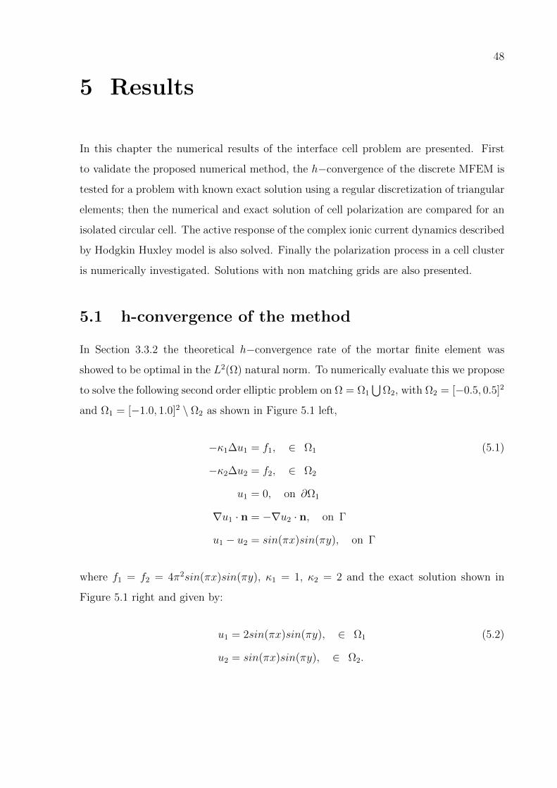
∇u1 · n = −∇u2 · n, on Γ
u1 − u2 = sin(πx)sin(πy), on Γ
where f1 = f2 = 4π2sin(πx)sin(πy), κ1 = 1, κ2 = 2 and the exact solution shown in
Figure 5.1 right and given by:
u1 = 2sin(πx)sin(πy), ∈ Ω1 (5.2)
u2 = sin(πx)sin(πy), ∈ Ω2.
49
Following the procedure exposed in Section 3.3, the discrete version of the variational
formulation of problem 5.1 can be loosely written,
κ
∫Ω
∇uh · ∇vhdx+
∫Γ
λh[vh]ds =
∫Ω
fvhdx, ∀vh ∈ Xh (5.3)
−∫
Γ
µh[uh]ds =
∫Γ
µhsin(πx)sin(πy)ds, ∀µh ∈Mh
u1 = 0, on ΓD
with κ = (κ1, κ2), Ω = Ω1
⋃Ω2 and f = (f1, f2).
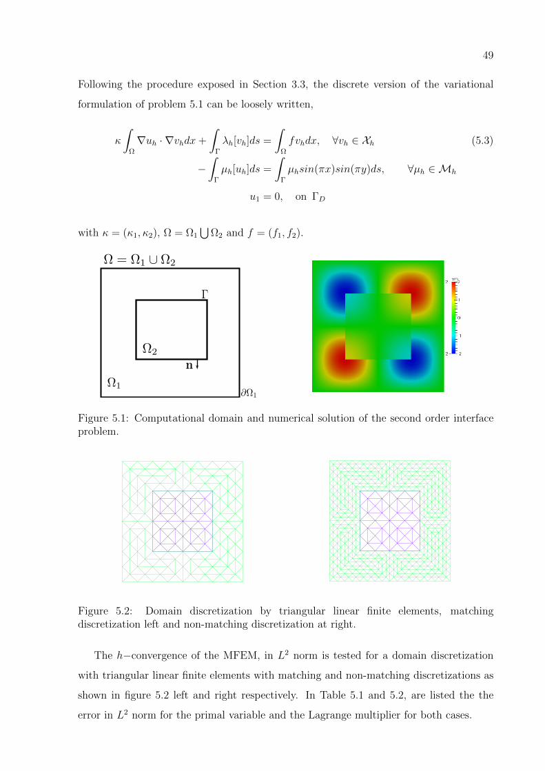
Figure 5.1: Computational domain and numerical solution of the second order interfaceproblem.
Figure 5.2: Domain discretization by triangular linear finite elements, matchingdiscretization left and non-matching discretization at right.
The h−convergence of the MFEM, in L2 norm is tested for a domain discretization
with triangular linear finite elements with matching and non-matching discretizations as
shown in figure 5.2 left and right respectively. In Table 5.1 and 5.2, are listed the the
error in L2 norm for the primal variable and the Lagrange multiplier for both cases.
50
‖u− uh‖L2(Ω) ‖λ− λh‖L2(Ω)
mesh error order error order16 1.12e-1 – 6.13e-1 –32 3.48e-2 1.68 3.99e-1 0.6264 9.24e-3 1.79 1.70e-1 0.93128 2.36e-3 1.86 7.80e-2 1.02256 5.96e-4 1.90 2.59e-2 1.15
Table 5.1: h−convergence order for the approximation of uh and λh obtained by theMFEM for matching triangular elements.
‖u− uh‖L2(Ω) ‖λ− λh‖L2(Ω)
mesh error order error order24 6.79e-2 – 4.87e-1 –48 2.23e-2 1.61 3.66e-1 0.8996 6.20e-3 1.73 2.12e-1 1.05192 1.61e-3 1.80 1.11e-1 1.09
Table 5.2: h−convergence order for the approximation of uh and λh obtained by theMFEM for non-matching triangular elements.
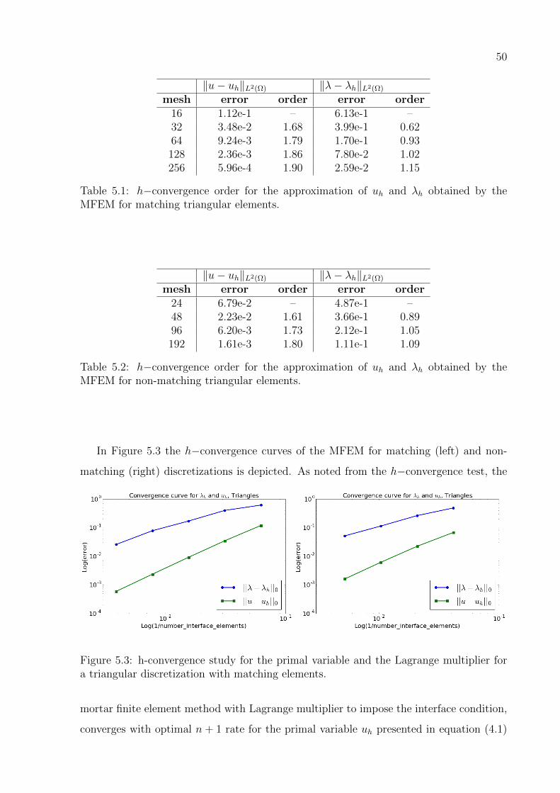
In Figure 5.3 the h−convergence curves of the MFEM for matching (left) and non-
matching (right) discretizations is depicted. As noted from the h−convergence test, the
Figure 5.3: h-convergence study for the primal variable and the Lagrange multiplier fora triangular discretization with matching elements.
mortar finite element method with Lagrange multiplier to impose the interface condition,
converges with optimal n + 1 rate for the primal variable uh presented in equation (4.1)
51
and with optimal rate n for the Lagrange multiplier λh. In the next section the cell
polarization and the active response of the cell membrane is investigated with the MFEM
with Lagrange multiplier.
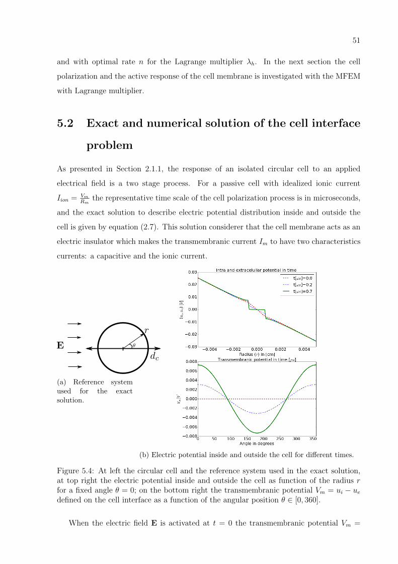
5.2 Exact and numerical solution of the cell interface
problem
As presented in Section 2.1.1, the response of an isolated circular cell to an applied
electrical field is a two stage process. For a passive cell with idealized ionic current
Iion = VmRm
the representative time scale of the cell polarization process is in microseconds,
and the exact solution to describe electric potential distribution inside and outside the
cell is given by equation (2.7). This solution considerer that the cell membrane acts as an
electric insulator which makes the transmembranic current Im to have two characteristics
currents: a capacitive and the ionic current.
(a) Reference systemused for the exactsolution.
(b) Electric potential inside and outside the cell for different times.
Figure 5.4: At left the circular cell and the reference system used in the exact solution,at top right the electric potential inside and outside the cell as function of the radius rfor a fixed angle θ = 0; on the bottom right the transmembranic potential Vm = ui − uedefined on the cell interface as a function of the angular position θ ∈ [0, 360].
When the electric field E is activated at t = 0 the transmembranic potential Vm =
52
ui−ue, on Γ is zero, and the transmembranic current Im = λ reaches its highest value. As
mentioned in Section 3.4 the initial value problem for the transmembranic potential (3.38)
is directly proportional to the transmembranic current Im. For a passive cell with idealized
ionic current Iion = VmRm
the polarization process takes place at time scale of microseconds
and finishes once the cell is totally polarized and equivalently the transmembranic current
is zero. Figure 5.4 shows right the exact solution of the electric potential distribution at
different time instants.
The exact solution presented in Figure 5.4 is for a circular cell of diameter dc = 15[µm]
the intra and extracellular conductance are κi = 5[mS · cm−1] and κe = 20[mS · cm−1]; the
membrane capacitance is Cm = 1[µF ·cm−2], the membrane resistance is Rm = 1KΩ ·cm2,
the applied electric field is E = 5V · cm−1 and the transmembranic current is measured in
Im[µA·cm−2] to preserve dimensional consistency. As noted from Figure 5.4 right, at t = 0
the transmembranic potential is zero and the electric potential distribution is uniform due
to the capacitive characteristic of the membrane, the transmembranic potential increase
proportionally to the transmembranic current, this causes the cell to create polar sides
facing the cathode and anode of the electrodes applying the electric field. As the time
passes the transmembranic current is consumed in form of potential difference between
the intra and extracellular medium. The cell polarization finish once the transmembranic
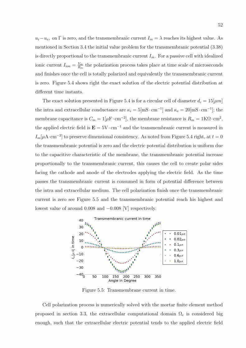
current is zero see Figure 5.5 and the transmembranic potential reach his highest and
lowest value of around 0.008 and −0.008 [V] respectively.
Figure 5.5: Transmembrane current in time.
Cell polarization process is numerically solved with the mortar finite element method
proposed in section 3.3, the extracellular computational domain Ωe is considered big
enough, such that the extracellular electric potential tends to the applied electric field
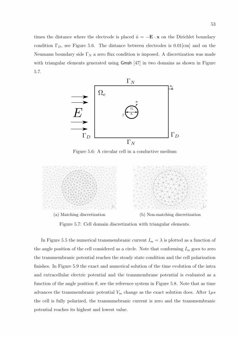
53
times the distance where the electrode is placed u = −E · x on the Dirichlet boundary
condition ΓD, see Figure 5.6. The distance between electrodes is 0.01[cm] and on the
Neumann boundary side ΓN a zero flux condition is imposed. A discretization was made
with triangular elements generated using Gmsh [47] in two domains as shown in Figure
5.7.
Figure 5.6: A circular cell in a conductive medium
X
Y
Z
(a) Matching discretization
X
Y
Z
(b) Non-matching discretization
Figure 5.7: Cell domain discretization with triangular elements.
In Figure 5.5 the numerical transmembranic current Im = λ is plotted as a function of
the angle position of the cell considered as a circle. Note that conforming Im goes to zero
the transmembranic potential reaches the steady state condition and the cell polarization
finishes. In Figure 5.9 the exact and numerical solution of the time evolution of the intra
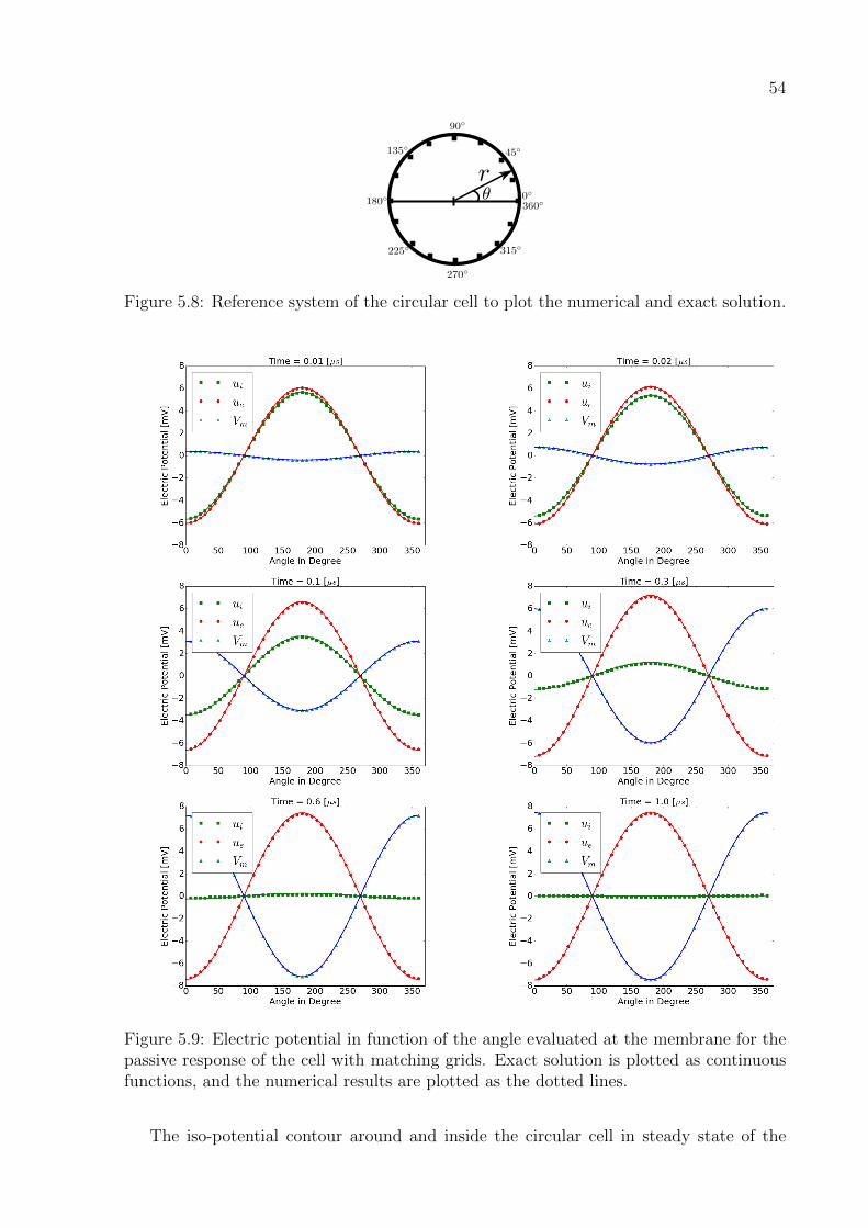
and extracellular electric potential and the transmembrane potential is evaluated as a
function of the angle position θ, see the reference system in Figure 5.8. Note that as time
advances the transmembranic potential Vm change as the exact solution does. After 1µs
the cell is fully polarized, the transmmebranic current is zero and the transmembranic
potential reaches its highest and lowest value.
54
Figure 5.8: Reference system of the circular cell to plot the numerical and exact solution.
Figure 5.9: Electric potential in function of the angle evaluated at the membrane for thepassive response of the cell with matching grids. Exact solution is plotted as continuousfunctions, and the numerical results are plotted as the dotted lines.
The iso-potential contour around and inside the circular cell in steady state of the
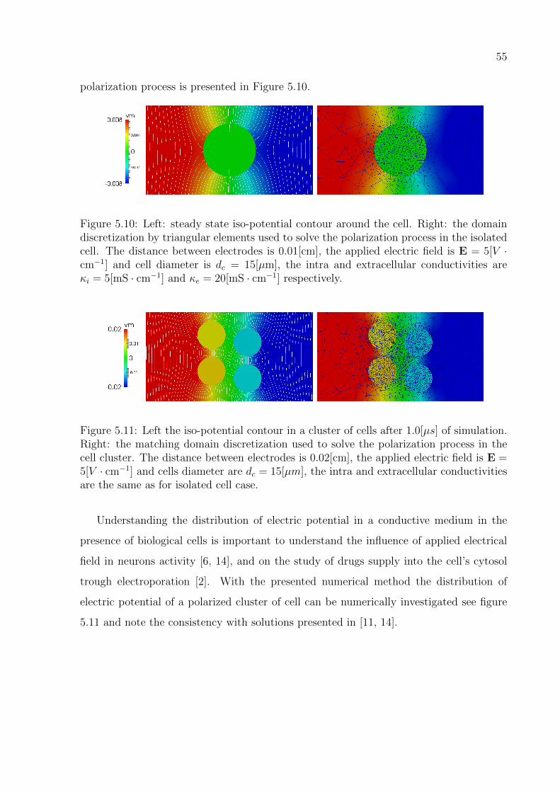
55
polarization process is presented in Figure 5.10.
Figure 5.10: Left: steady state iso-potential contour around the cell. Right: the domaindiscretization by triangular elements used to solve the polarization process in the isolatedcell. The distance between electrodes is 0.01[cm], the applied electric field is E = 5[V ·cm−1] and cell diameter is dc = 15[µm], the intra and extracellular conductivities areκi = 5[mS · cm−1] and κe = 20[mS · cm−1] respectively.
Figure 5.11: Left the iso-potential contour in a cluster of cells after 1.0[µs] of simulation.Right: the matching domain discretization used to solve the polarization process in thecell cluster. The distance between electrodes is 0.02[cm], the applied electric field is E =5[V · cm−1] and cells diameter are dc = 15[µm], the intra and extracellular conductivitiesare the same as for isolated cell case.
Understanding the distribution of electric potential in a conductive medium in the
presence of biological cells is important to understand the influence of applied electrical
field in neurons activity [6, 14], and on the study of drugs supply into the cell’s cytosol
trough electroporation [2]. With the presented numerical method the distribution of
electric potential of a polarized cluster of cell can be numerically investigated see figure
5.11 and note the consistency with solutions presented in [11, 14].
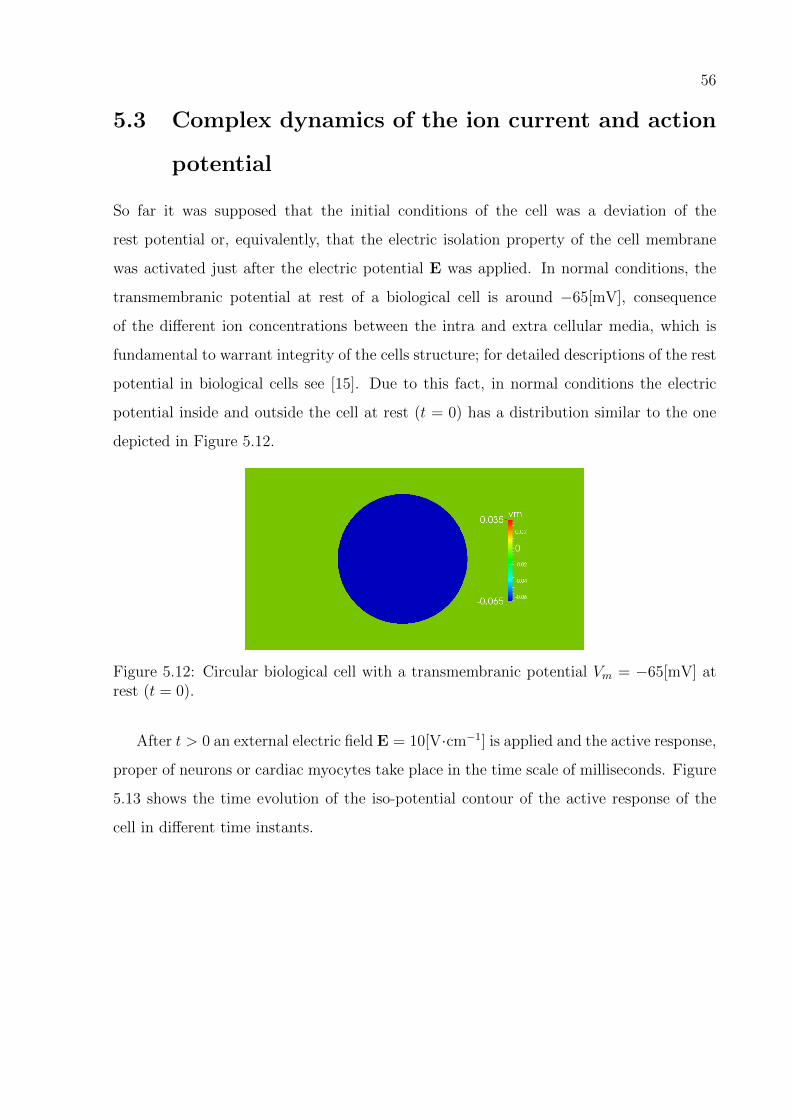
56
5.3 Complex dynamics of the ion current and action
potential
So far it was supposed that the initial conditions of the cell was a deviation of the
rest potential or, equivalently, that the electric isolation property of the cell membrane
was activated just after the electric potential E was applied. In normal conditions, the
transmembranic potential at rest of a biological cell is around −65[mV], consequence
of the different ion concentrations between the intra and extra cellular media, which is
fundamental to warrant integrity of the cells structure; for detailed descriptions of the rest
potential in biological cells see [15]. Due to this fact, in normal conditions the electric
potential inside and outside the cell at rest (t = 0) has a distribution similar to the one
depicted in Figure 5.12.
Figure 5.12: Circular biological cell with a transmembranic potential Vm = −65[mV] atrest (t = 0).
After t > 0 an external electric field E = 10[V·cm−1] is applied and the active response,
proper of neurons or cardiac myocytes take place in the time scale of milliseconds. Figure
5.13 shows the time evolution of the iso-potential contour of the active response of the
cell in different time instants.
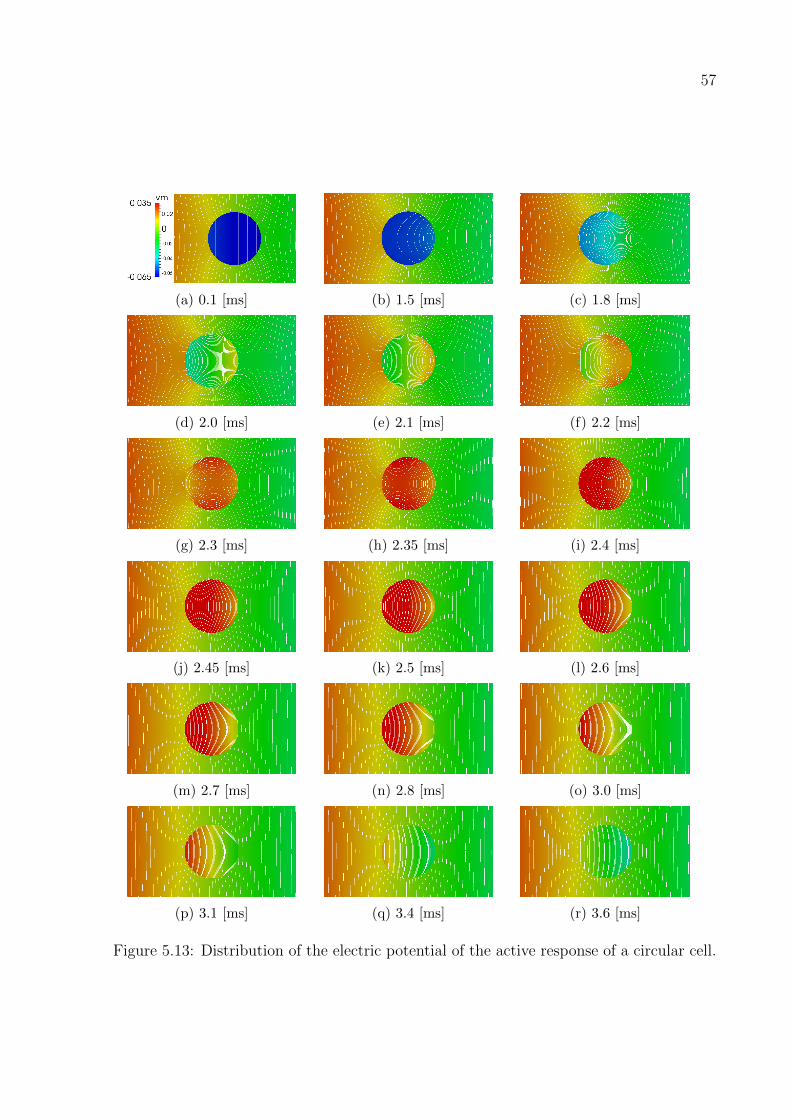
57
(a) 0.1 [ms] (b) 1.5 [ms] (c) 1.8 [ms]
(d) 2.0 [ms] (e) 2.1 [ms] (f) 2.2 [ms]
(g) 2.3 [ms] (h) 2.35 [ms] (i) 2.4 [ms]
(j) 2.45 [ms] (k) 2.5 [ms] (l) 2.6 [ms]
(m) 2.7 [ms] (n) 2.8 [ms] (o) 3.0 [ms]
(p) 3.1 [ms] (q) 3.4 [ms] (r) 3.6 [ms]
Figure 5.13: Distribution of the electric potential of the active response of a circular cell.
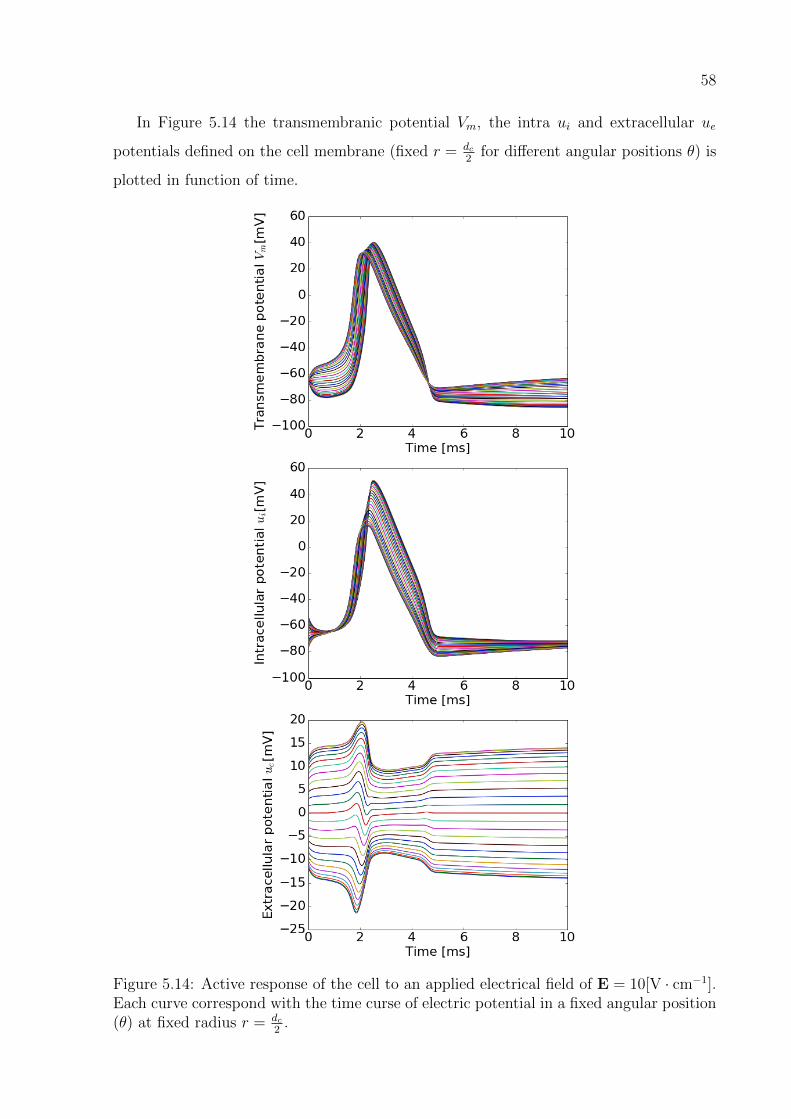
58
In Figure 5.14 the transmembranic potential Vm, the intra ui and extracellular ue
potentials defined on the cell membrane (fixed r = dc2
for different angular positions θ) is
plotted in function of time.
Figure 5.14: Active response of the cell to an applied electrical field of E = 10[V · cm−1].Each curve correspond with the time curse of electric potential in a fixed angular position(θ) at fixed radius r = dc
2.
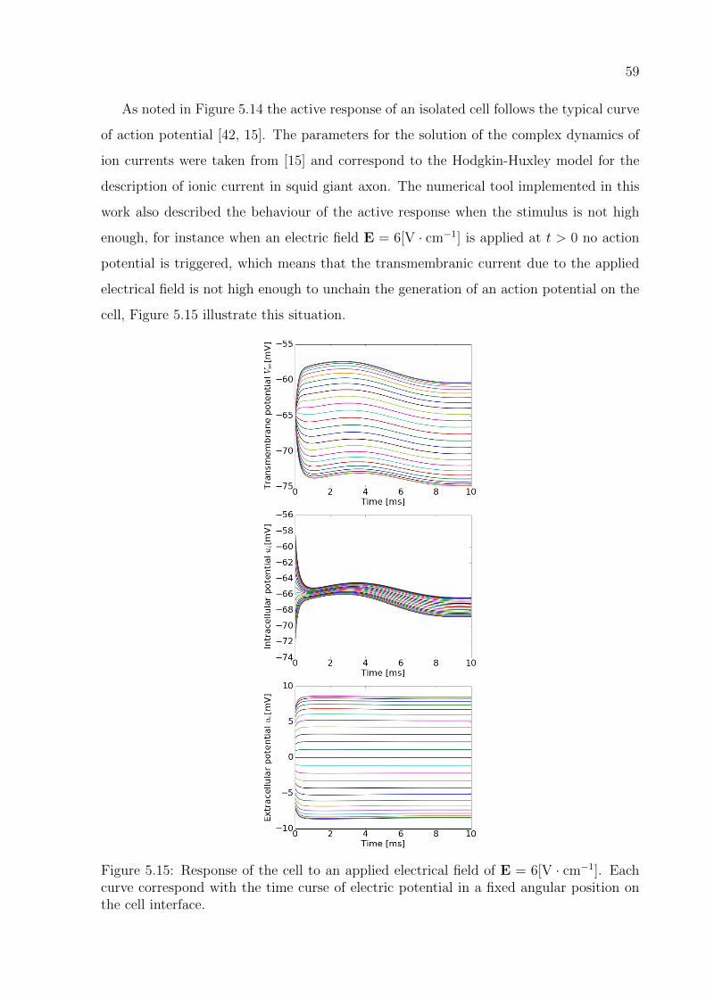
59
As noted in Figure 5.14 the active response of an isolated cell follows the typical curve
of action potential [42, 15]. The parameters for the solution of the complex dynamics of
ion currents were taken from [15] and correspond to the Hodgkin-Huxley model for the
description of ionic current in squid giant axon. The numerical tool implemented in this
work also described the behaviour of the active response when the stimulus is not high
enough, for instance when an electric field E = 6[V · cm−1] is applied at t > 0 no action
potential is triggered, which means that the transmembranic current due to the applied
electrical field is not high enough to unchain the generation of an action potential on the
cell, Figure 5.15 illustrate this situation.
Figure 5.15: Response of the cell to an applied electrical field of E = 6[V · cm−1]. Eachcurve correspond with the time curse of electric potential in a fixed angular position onthe cell interface.
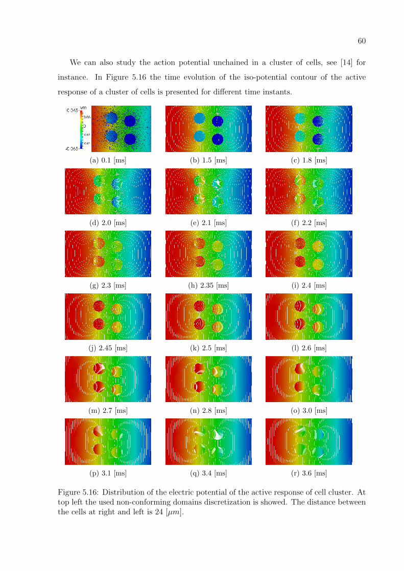
60
We can also study the action potential unchained in a cluster of cells, see [14] for
instance. In Figure 5.16 the time evolution of the iso-potential contour of the active
response of a cluster of cells is presented for different time instants.
(a) 0.1 [ms] (b) 1.5 [ms] (c) 1.8 [ms]
(d) 2.0 [ms] (e) 2.1 [ms] (f) 2.2 [ms]
(g) 2.3 [ms] (h) 2.35 [ms] (i) 2.4 [ms]
(j) 2.45 [ms] (k) 2.5 [ms] (l) 2.6 [ms]
(m) 2.7 [ms] (n) 2.8 [ms] (o) 3.0 [ms]
(p) 3.1 [ms] (q) 3.4 [ms] (r) 3.6 [ms]
Figure 5.16: Distribution of the electric potential of the active response of cell cluster. Attop left the used non-conforming domains discretization is showed. The distance betweenthe cells at right and left is 24 [µm].
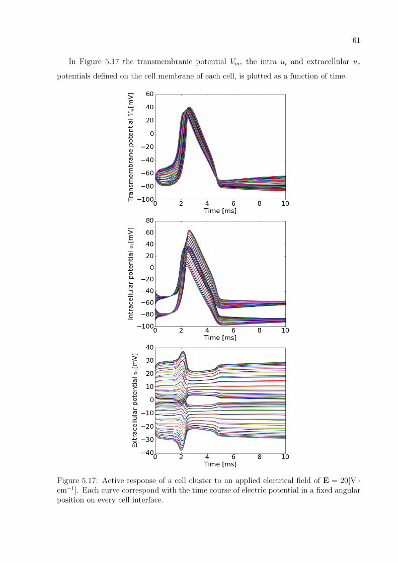
61
In Figure 5.17 the transmembranic potential Vm, the intra ui and extracellular ue
potentials defined on the cell membrane of each cell, is plotted as a function of time.
Figure 5.17: Active response of a cell cluster to an applied electrical field of E = 20[V ·cm−1]. Each curve correspond with the time course of electric potential in a fixed angularposition on every cell interface.
62
6 Conclusions
In this work a Mortar Finite Element Method MFEM was effectively developed and used
to numerically investigate the active and passive response of an isolated cell and cluster
of cells to an applied electric field. The approximation properties of the MFEM were
conforming with the results of the specialized literature, that is, optimal h-convergence
order for the primal variable and the Lagrange multiplier for both the matching and
non-matching domain discretization.
A hybrid variational formulation was effectively used to decoupled the boundary
value problem describing the electric current conservation from the initial value problem
describing the passive and the complex active response of the biological cell to applied
field. The hybrid variational formulation effectively solved the cell interface problem,
allowing to have discontinuous solutions in the computational domain without the need
of having refined domain discretization to interpolate the solution. Therefore we conclude
that the MFEM based on hybrid variational formulation is an elegant method to solve
interface problems with complex dynamics.
The complex active response described by the Hodgkin-Huxley HH model of a cell
and a cluster of cells to an applied electrical field was effectively solved via MFEM. It was
found that the numerical tool reproduces the experimental behaviour in both cases, when
the transmembranic current is high enough to generate action potential and also when it
is not; due to the spatial resolution of the numerical tool a more detailed description of
the action potential described by the HH model was obtained.
The most important product of this work is the extension of the Cardiax FEM library
to solve second order heterogeneous interface problems with discontinuous solutions on
the domain with conforming and non-conforming discretized domains via triangular finite
elements.
During the development of this work, it was encountered that the Krylov subspace
method MINRES together with a Jacobi preconditioner was the most robust method to
solve the indefinite linear system associated to the discrete version of the saddle point
problem encountered in the MFEM.
63
6.1 Future works
During the development of this work, alternative variational formulations were sketched
on the paper but not implemented. In this sense, one possibility is to include GLS
stabilization terms to the hybrid variational formulation, which generate a symmetric
positive defined linear system suitable to solve with the conjugate gradient method
or matrix decomposition methods as LU. Another interesting variational formulation
appropriate for the cell interface problem, is a hybrid version of a mixed formulation.
In theory this approach will allow to have optimal n + 1 h-convergence for both the
primal variable and the Lagrange multiplier, highly beneficial for the cell interface problem
because of the improvement in the approximation order for the Lagrange multiplier used
in the solution of the initial value problem. It is also proposed as future work the
implementation of higher order mortar finite elements.
64
REFERENCES
[1] ORLOWSKI, S., MIR, L. M., “Cell electropermeabilization: a new tool for biochemical
and pharmacological studies”, Biochimica et Biophysica Acta (BBA)-Reviews
on Biomembranes , v. 1154, n. 1, pp. 51–63, 1993.
[2] CHEN, C., SMYE, S., ROBINSON, M., EVANS, J., “Membrane electroporation
theories: a review”, Medical and Biological Engineering and Computing , v. 44,
n. 1, pp. 5–14, 2006.
[3] ASHIHARA, T., YAO, T., NAMBA, T., ITO, M., IKEDA, T., KAWASE, A.,
TODA, S., SUZUKI, T., INAGAKI, M., SUGIMACHI, M., KINOSHITA,
M., NAKAZAWA, K., “Electroporation in a Model of Cardiac Defibrillation”,
Journal of Cardiovascular Electrophysiology , v. 12, n. 12, pp. 1393–1403, 2001.
[4] KRASSOWSKA, W., “Effects of Electroporation on Transmembrane Potential
Induced by Defibrillation Shocks”, Pacing and Clinical Electrophysiology , v. 18,
n. 9, pp. 1644–1660, 1995.
[5] NIKOLSKI, V. P., EFIMOV, I. R., “Electroporation of the heart”, EP Europace, v. 7,
n. s2, pp. S146, 2005.
[6] AGUDELO-TORO, A., NEEF, A., “Computationally efficient simulation of electrical
activity at cell membranes interacting with self-generated and externally
imposed electric fields”, Journal of Neural Engineering , v. 10, n. 2, pp. 026019,
2013.
[7] KRASSOWSKA, W., NEU, J., “Response of a single cell to an external electric field”,
Biophysical Journal , v. 66, n. 6, pp. 1768 – 1776, 1994.
[8] GIMSA, J., WACHNER, D., “Analytical description of the transmembrane voltage
induced on arbitrarily oriented ellipsoidal and cylindrical cells”, Biophysical
Journal , v. 81, n. 4, pp. 1888–1896, 2001.
[9] VALIC, B., GOLZIO, M., PAVLIN, M., SCHATZ, A., FAURIE, C., GABRIEL,
B., TEISSIE, J., ROLS, M.-P., MIKLAVCIC, D., “Effect of electric field
induced transmembrane potential on spheroidal cells: theory and experiment”,
European Biophysics Journal , v. 32, n. 6, pp. 519–528, Oct 2003.
65
[10] LEE, D. C., GRILL, W. M., “Polarization of a Spherical Cell in a Nonuniform
Extracellular Electric Field”, Annals of Biomedical Engineering , v. 33, n. 5,
pp. 603–615, 2005.
[11] YING, W., HENRIQUEZ, C. S., “Hybrid finite element method for describing the
electrical response of biological cells to applied fields”, IEEE Transactions on
Biomedical Engineering , v. 54, n. 4, pp. 611–620, 2007.
[12] PUCIHAR, G., MIKLAVCIC, D., KOTNIK, T., “A time-dependent numerical model
of transmembrane voltage inducement and electroporation of irregularly shaped
cells”, IEEE Transactions on Biomedical Engineering , v. 56, n. 5, pp. 1491–
1501, 2009.
[13] SUSIL, R., SEMROV, D., MIKLAVCIC, D., “Electric Field-Induced Transmembrane
Potential Depends on Cell Density and Organizatio”, Electro-and
magnetobiology , v. 17, n. 3, pp. 391–399, 1998.
[14] YING, W., POURTAHERI, N., HENRIQUEZ, C. S., “Field stimulation of cells in
suspension: use of a hybrid finite element method”. In: Engineering in Medicine
and Biology Society, 2006. EMBS’06. 28th Annual International Conference of
the IEEE , pp. 2276–2279, 2006.
[15] KEENER, J., SNEYD, J., Mathematical physiology: I: cellular physiology . Springer
Science & Business Media, 2010.
[16] SEMROV, D., MIKLAVCIC, D., “Numerical Modeling for In Vivo Electroporation”,
In: JAROSZESKI, M. J., HELLER, R., GILBERT, R. (eds),
Electrochemotherapy, Electrogenetherapy, and Transdermal Drug Delivery:
Electrically Mediated Delivery of Molecules to Cells , pp. 63–81, Humana Press:
Totowa, NJ, 2000.
[17] CIARLET, P., KESAVAN, S., RANJAN, A., VANNINATHAN, M., Lectures on the
Finite Element Method . Lectures on mathematics and physics: Mathematics ,
Tata Institute of Fundamental Research, 1975.
66
[18] RAVIART, P.-A., THOMAS, J.-M., CIARLET, P. G., LIONS, J. L., Introduction a
l’analyse numerique des equations aux derivees partielles . v. 2. Dunod Paris,
1998.
[19] RAVIART, P.-A., THOMAS, J., “Primal hybrid finite element methods for 2nd order
elliptic equations”, Mathematics of computation, v. 31, n. 138, pp. 391–413,
1977.
[20] BERNARDI, C., MADAY, Y., PATERA, A. T., “Domain Decomposition by the
Mortar Element Method”, In: KAPER, H. G., GARBEY, M., PIEPER,
G. W. (eds), Asymptotic and Numerical Methods for Partial Differential
Equations with Critical Parameters , pp. 269–286, Springer Netherlands:
Dordrecht, 1993.
[21] BELGACEM, F. B., “The Mortar finite element method with Lagrange multipliers”,
Numerische Mathematik , v. 84, n. 2, pp. 173–197, 1999.
[22] WOHLMUTH, B. I., “A Mortar Finite Element Method Using Dual Spaces for
the Lagrange Multiplier”, SIAM Journal on Numerical Analysis , v. 38, n. 3,
pp. 989–1012, 2000.
[23] LAMICHHANE, B. P., “Higher order mortar finite elements with dual Lagrange
multiplier spaces and applications”, 2006.
[24] BENZI, M., GOLUB, G. H., LIESEN, J., “Numerical solution of saddle point
problems”, Acta numerica, v. 14, pp. 1–137, 2005.
[25] BARBOSA, H. J., HUGHES, T. J., “The finite element method with Lagrange
multipliers on the boundary: circumventing the Babuska-Brezzi condition”,
Computer Methods in Applied Mechanics and Engineering , v. 85, n. 1, pp. 109–
128, 1991.
[26] BAIOCCHI, C., BREZZI, F., MARINI, L. D., “Stabilization of Galerkin methods
and applications to domain decomposition”, In: BENSOUSSAN, A.,
VERJUS, J. P. (eds), Future Tendencies in Computer Science, Control and
Applied Mathematics: International Conference on the Occasion of the 25th
67
Anniversary of INRIA Paris, France, December 8–11, 1992 Proceedings , pp.
343–355, Springer Berlin Heidelberg: Berlin, Heidelberg, 1992.
[27] EWING, R. E., WANG, J., YANG, Y., “A stabilized discontinuous finite element
method for elliptic problems”, Numerical Linear Algebra with Applications ,
v. 10, n. 1-2, pp. 83–104, 2003.
[28] BRAESS, D., DAHMEN, W., WIENERS, C., “A Multigrid Algorithm for the Mortar
Finite Element Method”, SIAM Journal on Numerical Analysis , v. 37, n. 1,
pp. 48–69, 1999.
[29] BREZZI, F., MARINI, L. D., “A three-field domain decomposition method”,
Contemporary Mathematics , v. 157, pp. 27–27, 1994.
[30] BERTOLUZZA, S., “Analysis of a mesh-dependent stabilization for the three fields
domain decomposition method”, Numerische Mathematik , v. 133, n. 1, pp. 1–
36, 2016.
[31] RAVIART, P., THOMAS, J., “A mixed finite element method for 2-nd order elliptic
problems”, Mathematical aspects of finite element methods , pp. 292–315, 1977.
[32] BREZZI, F., FORTIN, M., Mixed and Hybrid Finite Element Methods . Springer-
Verlag New York, Inc.: New York, NY, USA, 1991.
[33] ARNOLD, D. N., BREZZI, F., “Mixed and nonconforming finite element methods
: implementation, postprocessing and error estimates”, ESAIM: M2AN , v. 19,
n. 1, pp. 7–32, 1985.
[34] BABUSKA, I., “The Finite Element Method with Penalty”, Mathematics of
Computation, v. 27, n. 122, pp. 221–228, 1973.
[35] NITSCHE, J., “Uber ein Variationsprinzip zur Losung von Dirichlet-Problemen bei
Verwendung von Teilraumen, die keinen Randbedingungen unterworfen sind”.
In: Abhandlungen aus dem mathematischen Seminar der Universitat Hamburg ,
v. 36, n. 1, pp. 9–15, 1971.
[36] ARNOLD, D. N., BREZZI, F., COCKBURN, B., MARINI, L. D., “Unified Analysis
of Discontinuous Galerkin Methods for Elliptic Problems”, SIAM Journal on
Numerical Analysis , v. 39, n. 5, pp. 1749–1779, 2002.
68
[37] COCKBURN, B., “Discontinuous Galerkin Methods for Convection-Dominated
Problems”, In: BARTH, T. J., DECONINCK, H. (eds), High-Order Methods
for Computational Physics , pp. 69–224, Springer Berlin Heidelberg: Berlin,
Heidelberg, 1999.
[38] COCKBURN, B., GOPALAKRISHNAN, J., LAZAROV, R., “Unified Hybridization
of Discontinuous Galerkin, Mixed, and Continuous Galerkin Methods for
Second Order Elliptic Problems”, SIAM Journal on Numerical Analysis , v. 47,
n. 2, pp. 1319–1365, 2009.
[39] EGGER, H., “A class of hybrid mortar finite element methods for interface problems
with non-matching meshes, 2009”, Preprint: AICES-2009-2 .
[40] ARRUDA, N. C., LOULA, A. F., ALMEIDA, R. C., “Locally discontinuous but
globally continuous Galerkin methods for elliptic problems”, Computer Methods
in Applied Mechanics and Engineering , v. 255, n. Supplement C, pp. 104 – 120,
2013.
[41] PLONSEY, R., HEPPNER, D. B., “Considerations of quasi-stationarity in
electrophysiological systems”, The bulletin of mathematical biophysics , v. 29,
n. 4, pp. 657–664, Dec 1967.
[42] HODGKIN, A. L., HUXLEY, A. F., “A quantitative description of membrane current
and its application to conduction and excitation in nerve”, The Journal of
Physiology , v. 117, n. 4, pp. 500–544, 1952.
[43] BREZZI, F., “On the existence, uniqueness and approximation of saddle-point
problems arising from lagrangian multipliers”, ESAIM: Mathematical Modelling
and Numerical Analysis - Modelisation Mathematique et Analyse Numerique,
v. 8, n. R2, pp. 129–151, 1974.
[44] PAIGE, C. C., SAUNDERS, M. A., “Solution of sparse indefinite systems of linear
equations”, SIAM journal on numerical analysis , v. 12, n. 4, pp. 617–629, 1975.
[45] CAMPOS, J. O., W. DOS SANTOS, R., SUNDNES, J., ROCHA, B. M.,
“Preconditioned Augmented Lagrangian formulation for nearly incompressible
69
cardiac mechanics”, International Journal for Numerical Methods in Biomedical
Engineering , cnm.2948.
[46] BALAY, S., ABHYANKAR, S., ADAMS, M. F., BROWN, J., BRUNE, P.,
BUSCHELMAN, K., DALCIN, L., EIJKHOUT, V., GROPP, W. D.,
KAUSHIK, D., KNEPLEY, M. G., MCINNES, L. C., RUPP, K., SMITH,
B. F., ZAMPINI, S., ZHANG, H., ZHANG, H., “PETSc Web page”, http:
//www.mcs.anl.gov/petsc, 2016.
[47] GEUZAINE, C., REMACLE, J.-F., “Gmsh: A 3-D finite element mesh generator
with built-in pre-and post-processing facilities”, International journal for
numerical methods in engineering , v. 79, n. 11, pp. 1309–1331, 2009.
Recommended