American Institute of Aeronautics and Astronautics
1
CFD Solver Comparison of Low Mach Flow over the
ROBIN Fuselage
Jennifer N. Abras1
NAVAIR Applied Aerodynamics and Store Separation Branch, Patuxent River, MD, 20670
and
Nathan Hariharan2
CREATE-AV, Lorton, VA, 22079
The ROtor Body INteraction (ROBIN) fuselage is used as a baseline test case for a
computational fluid dynamic (CFD) study of solver drag prediction results for low Mach
flow. All of the predictions are compared not only to one another, but also to available wind
tunnel data. Comparisons of integrated viscous and pressure drag, flow separation point,
and centerline pressure distributions are analyzed. Parametric studies of the independent
options available within each code for low Mach flow conditions are investigated. Grid
studies are also presented. The final comparisons reveal that for the attached flow regions
all of the CFD codes predict approximately the same result. The differences occur when the
flow begins to separate aft of the fuselage. Benefits are gained when the viscous grid layers
are merged from tetrahedrons into prisms, and when the incompressible option is employed.
Higher spatial order of accuracy in the separated region is found to slightly improve the
results.
I. Introduction
HE CREATE-AV program is focused on developing state-of-the-art software for use with both fixed wing and
rotary wing aircraft analysis. These codes are HPCMP CREATETM
-AV HELIOS for rotary wing analysis and
HPCMP CREATETM
-AV KESTREL for fixed wing analysis. Release versions of both of these codes are currently
in use in government, industry, and academia. However, the development process to expand the capabilities of these
codes and to improve on the present capabilities is ongoing. While these changes and improvements encompass a
wide range of topics, one specific area of improvement is the addition of a new near-body CFD solver in CREATE-
AV HELIOS.
Evaluation of major changes in the configuration of any CFD code are pursued through comparisons to both
available measured data as well as to the predictions produced by established CFD solvers. Planned changes to the
CREATE-AV HELIOS solver will be evaluated using these types of comparisons. The near-body CFD solver in the
current release version of CREATE-AV HELIOS, is NSU3D. Future versions of CREATE-AV HELIOS are
planned to transition to the kCFD solver which currently resides in CREATE-AV KESTREL. It is of interest to
compare both kCFD and NSU3D to better understand the possible impact that the transition will have on the
CREATE-AV HELIOS solver. Predictions from both of these codes will be compared not only to one another, but
also to available wind tunnel data and predictions from both the OVERFLOW and FUN3D solvers.
The wind tunnel test case selected for this comparison is centered around the ROBIN-mod7 isolated fuselage.
This test was run in the NASA Langley 2 ft x 3 ft wind tunnel. The purpose of this test is to investigate fuselage
drag reduction using aft blowing. However, the baseline cases run during this test are suitable for comparison
during the present study. Reference 1 contains a subset of the wind tunnel data from this test as well as the
OVERFLOW predictions. The outer mold line of this fuselage is defined by a series of equations that are provided
in appendix A of reference 1. All test data and OVERFLOW predictions presented herein have been digitized or
copied from this paper. Recent CREATE-AV HELIOS evaluations have also used this test data, comparing
CREATE-AV HELIOS to a commercial off the shelf (COTS) solver, CFD++2.
1 Aerospace Engineer, [email protected], AIAA Professional Member.
2 Deputy Project Manager, [email protected], AIAA Associate Fellow.
T
Dow
nloa
ded
by N
ASA
LA
NG
LE
Y R
ESE
AR
CH
CE
NT
RE
on
July
7, 2
015
| http
://ar
c.ai
aa.o
rg |
DO
I: 1
0.25
14/6
.201
4-07
52
52nd Aerospace Sciences Meeting
13-17 January 2014, National Harbor, Maryland
AIAA 2014-0752
This material is declared a work of the U.S. Government and is not subject to copyright protection in the United States.
AIAA SciTech
American Institute of Aeronautics and Astronautics
2
This paper compares the drag predictions of the CREATE-AV HELIOS solver and the CREATE-AV KESTREL
solver against available wind tunnel data and predictions made by OVERFLOW and FUN3D. These comparisons
include grid density studies, grid boundary layer analysis, incompressible solver evaluation, near-body trim distance
analysis, overall solver comparisons, and a timing and convergence comparison. The final comparisons utilize the
centerline pressure distributions, center slice velocity contours, flow separation location, and integrated pressure and
viscous drag coefficients in order to assess the performance of each code.
II. Methodology
A. HPCMP CREATETM
-AV HELIOS v4.0
CREATE-AV HELIOS3 is a multi-function code designed specifically for rotorcraft analysis. It contains
unstructured near-body and Cartesian off-body CFD solvers, overset methodology using PUNDIT, rigid grid
motion, and rotor blade structural deformations through RCAS or through prescribed deformations. The near-body
solver is NSU3D, a node-centered unstructured CFD code that solves the Reynolds Averaged Navier-Stokes
(RANS) equations applying 2nd
-order spatial accuracy. The Spalart-Allmaras (SA) and SA-DES turbulence models
are available. The unstructured grid can contain a mixture of tetrahedral and prismatic cells. ARC3D is the off-
body Cartesian solver which applies up to 5th
-order spatial accuracy. This solver may be run inviscid or with the
SA-DES turbulence model. This solver also has the option of applying automatic mesh refinement (AMR) to the
solution. Cases using NSU3D alone and dual NSU3D and ARC3D are presented. All cases apply the SA
turbulence model to the near-body, and the Euler solution in the off-body where applicable. All solutions are run
steady-state.
B. HPCMP CREATETM
-AV KESTREL v4.0.5
CREATE-AV KESTREL3 is a multi-function code designed specifically for fixed wing aircraft analysis. It
contains a near-body CFD solver (kCFD), control surface motion capability, engine analysis, and 6DoF analysis.
kCFD is a cell-centered unstructured CFD code which solves the RANS equation using 2nd
-order spatial accuracy.
A variety of turbulence models are available including the SA and SA-DDES models. The unstructured grid can
contain a mixture of tetrahedral and prismatic cells. This solver also has the option of applying automatic mesh
refinement (AMR) to the solution. All cases apply the SA turbulence model and are run steady-state.
C. FUN3D v12.2
The NASA Langley code FUN3D4
is an unstructured CFD code that solves the RANS equations using a node-
centered 2nd
-order upwind implicit scheme. The unstructured grid can contain a mixture of tetrahedral and prismatic
cells. This code is able to perform a variety of analyses including rigid and elastic grid motion, 6DoF analysis,
design optimization, and grid adaptation. This code also contains a variety of rotorcraft specific options including
coupling with external comprehensive rotorcraft codes. There are a wide variety of flux schemes and turbulence
models available, but for this study the Roe flux scheme and the SA turbulence model have been selected. All cases
are run steady-state.
III. Conditions
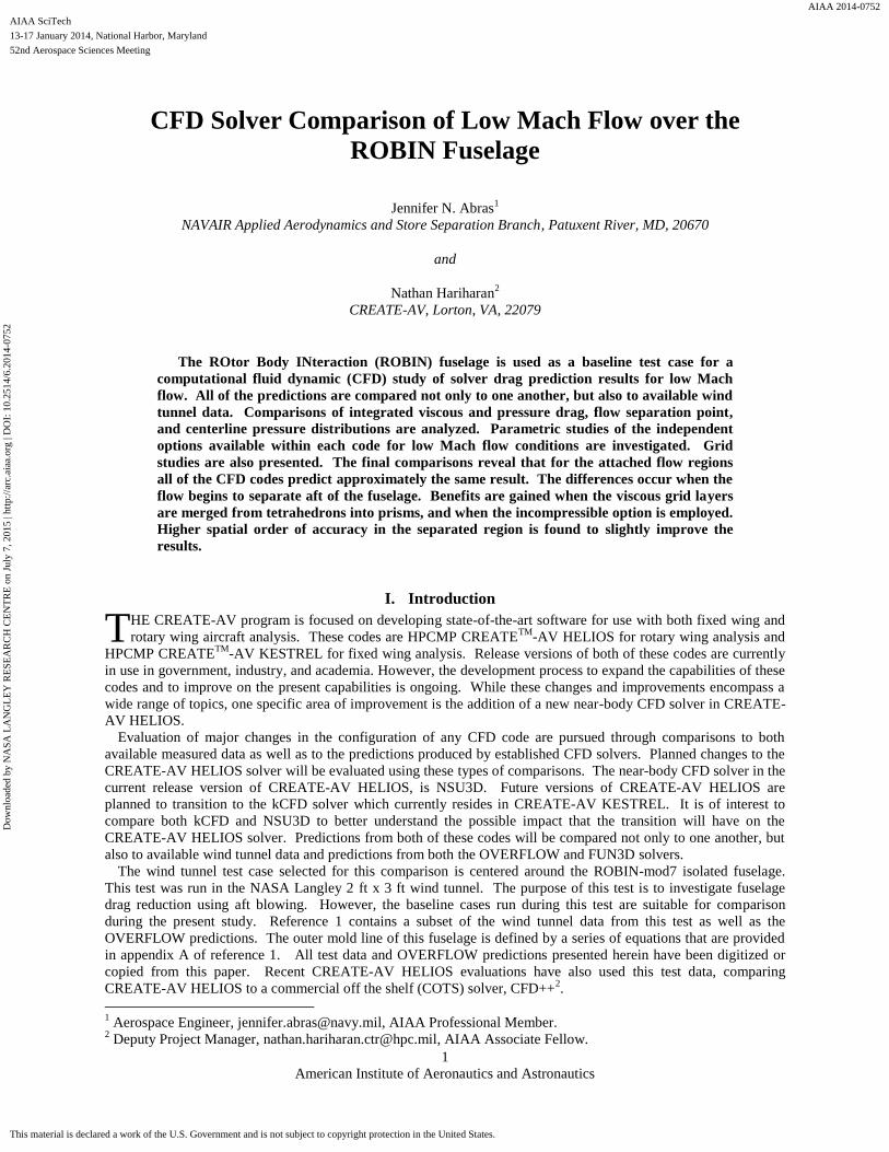
The wind tunnel model is shown in Figure 1. The
model is inverted in order to focus on the flow
separation on the lower aft portion of the fuselage. A
series of 41 pressure taps are located along the
centerline of the fuselage. These pressure taps run
along the length of the bottom of the fuselage, and
along the top of the fuselage between the nose and the
post. The flow conditions utilized include a Mach
number of 0.1 (about 34 m/s), a Reynolds number,
based on the fuselage length, of 1.6M and an angle of
attack of 0. Standard sea level conditions are
assumed in the CFD solutions. The mount shroud is
constructed using an extruded NACA0018 airfoil
section. Figure 1. Image of the wind tunnel model from Ref.1.
Dow
nloa
ded
by N
ASA
LA
NG
LE
Y R
ESE
AR
CH
CE
NT
RE
on
July
7, 2
015
| http
://ar
c.ai
aa.o
rg |
DO
I: 1
0.25
14/6
.201
4-07
52
American Institute of Aeronautics and Astronautics
3
IV. Grids
The underlying CAD used for this model is in the form of a NASTRAN file. This NASTRAN mesh data was
loaded into the Rhinoceros v4.0 CAD program where NURBS surfaces were generated. These NURBS surfaces
were used within the NASA Langley TetrUSS tools, GridTool and VGrid, to generate the tetrahedral unstructured
grids. All the solvers employed here use unstructured grids, the details for these grids are provided in Table 1. The
boundary layers are merged for a majority of the cases. This boundary layer merging is always performed using the
CREATE-AV HELIOS preprocessor. The resulting processed NSU3D grid is then used within CREATE-AV
KESTREL and FUN3D for consistency. For CREATE-AV KESTREL this grid is converted to AVMesh format
using the CREATE-AV KESTREL preprocessor, FUN3D is able to read in the NSU3D file format with no
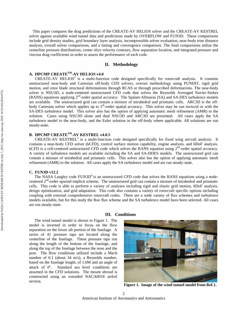
modification. Some CREATE-AV
HELIOS cases were run with an
unstructured near-body and a Cartesian
off-body. This grid (Grid-5) contains a
constant cell size with trim distances
ranging from 0.25 inches to 0.5 inches.
The first set of cases run use the ROBIN-
mod7 fuselage with a pylon on the top as
shown in Figure 2. The wind tunnel model
has this removed in order to add the
mount. The corresponding “free-air”
OVERFLOW predictions were run
without this pylon. Thus, a second series
of cases were run for each solver using the
model with no pylon. The boundary layer
spacing in all cases is selected to ensure
that the y+ value is less than one over the
entire fuselage.
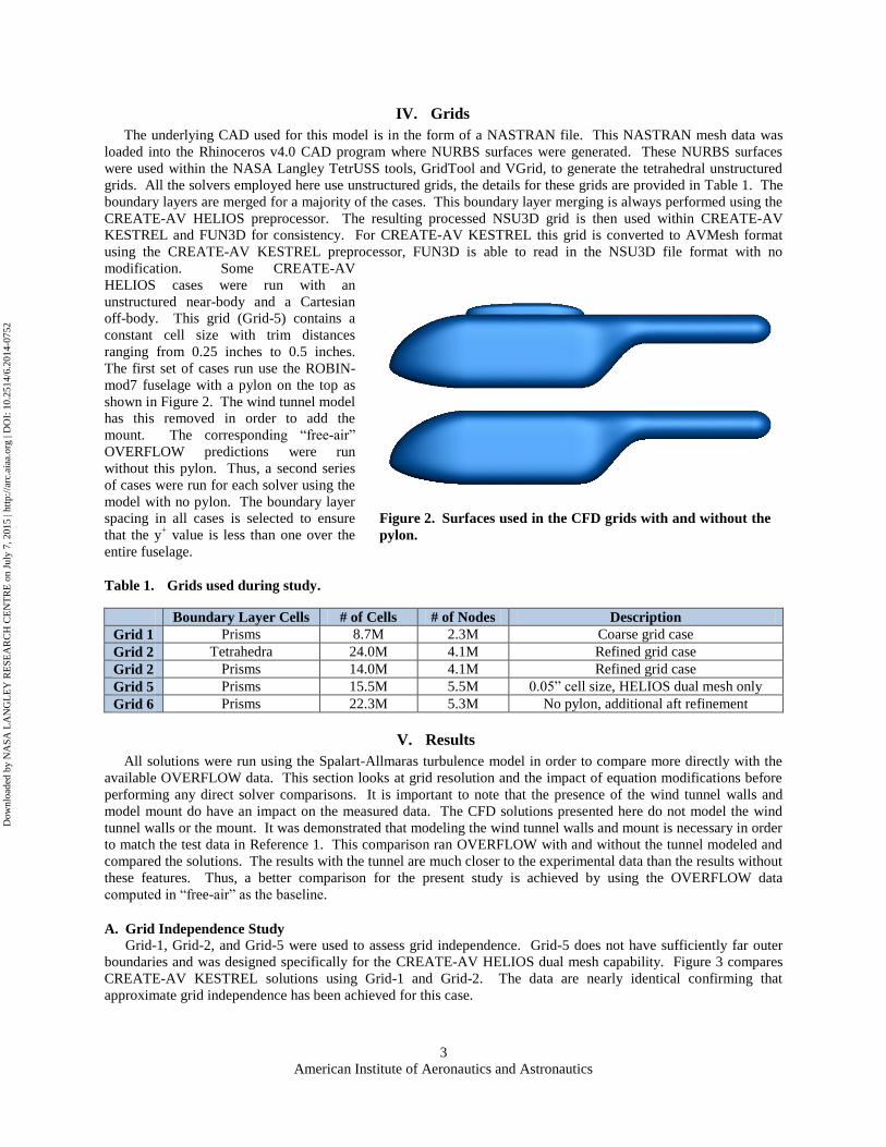
Table 1. Grids used during study.
Boundary Layer Cells # of Cells # of Nodes Description
Grid 1 Prisms 8.7M 2.3M Coarse grid case
Grid 2 Tetrahedra 24.0M 4.1M Refined grid case
Grid 2 Prisms 14.0M 4.1M Refined grid case
Grid 5 Prisms 15.5M 5.5M 0.05” cell size, HELIOS dual mesh only
Grid 6 Prisms 22.3M 5.3M No pylon, additional aft refinement
V. Results
All solutions were run using the Spalart-Allmaras turbulence model in order to compare more directly with the
available OVERFLOW data. This section looks at grid resolution and the impact of equation modifications before
performing any direct solver comparisons. It is important to note that the presence of the wind tunnel walls and
model mount do have an impact on the measured data. The CFD solutions presented here do not model the wind
tunnel walls or the mount. It was demonstrated that modeling the wind tunnel walls and mount is necessary in order
to match the test data in Reference 1. This comparison ran OVERFLOW with and without the tunnel modeled and
compared the solutions. The results with the tunnel are much closer to the experimental data than the results without
these features. Thus, a better comparison for the present study is achieved by using the OVERFLOW data
computed in “free-air” as the baseline.
A. Grid Independence Study
Grid-1, Grid-2, and Grid-5 were used to assess grid independence. Grid-5 does not have sufficiently far outer
boundaries and was designed specifically for the CREATE-AV HELIOS dual mesh capability. Figure 3 compares
CREATE-AV KESTREL solutions using Grid-1 and Grid-2. The data are nearly identical confirming that
approximate grid independence has been achieved for this case.
Figure 2. Surfaces used in the CFD grids with and without the
pylon.
Dow
nloa
ded
by N
ASA
LA
NG
LE
Y R
ESE
AR
CH
CE
NT
RE
on
July
7, 2
015
| http
://ar
c.ai
aa.o
rg |
DO
I: 1
0.25
14/6
.201
4-07
52

American Institute of Aeronautics and Astronautics
4
The CREATE-AV HELIOS grid comparisons are shown in Figure 4. The solutions reveal that for Grid-1 and
Grid-2 the solutions are nearly identical. This is also true of Grid-5 in the attached flow regions. However, there is
a large difference in the separated region when employing the dual mesh methodology with Grid-5. This is
hypothesized to be the result of having a finer off-body mesh in the region aft of the fuselage in the separated flow
region as well as having higher order spatial accuracy in the off-body solver. This hypothesis was partially tested by
creating an unstructured mesh (Grid-6) with additional refinement in the same aft region and running an isolated
NSU3D case on this mesh. The results do show some improvement in the separated region with the additional
refinement. It should be noted that the dual mesh case is not using the isolated NSU3D solver as is used for Grid-1
and Grid-2. The Grid-5 case uses a combined NSU3D/ARC3D solver where the ARC3D solver is applying the
Euler equations in the off-body.
-1
-0.5
0
0.5
1
1.5
2
0 0.2 0.4 0.6 0.8 1 1.2 1.4
Cp
x/R
Experiment TopHelios Grid 5Helios Grid 2Helios Grid 1
-1
-0.8
-0.6
-0.4
-0.2
0
0.2
0.4
0.6
0.8
1
0 0.2 0.4 0.6 0.8 1 1.2 1.4
Cp
x/R
Experiment BottomHelios Grid 5Helios Grid 2Helios Grid 1
Figure 4. Grid independence for CREATE-AV HELIOS solutions.
-1
-0.5
0
0.5
1
1.5
2
0 0.2 0.4 0.6 0.8 1 1.2 1.4
Cp
x/R
Experiment Top
Kestrel Grid 2
Kestrel Grid 1
-1
-0.8
-0.6
-0.4
-0.2
0
0.2
0.4
0.6
0.8
1
0 0.2 0.4 0.6 0.8 1 1.2 1.4
Cp
x/R
Experiment Bottom
Kestrel Grid 2
Kestrel Grid 1
Figure 3. Grid independence for CREATE-AV KESTREL solutions.
Dow
nloa
ded
by N
ASA
LA
NG
LE
Y R
ESE
AR
CH
CE
NT
RE
on
July
7, 2
015
| http
://ar
c.ai
aa.o
rg |
DO
I: 1
0.25
14/6
.201
4-07
52
American Institute of Aeronautics and Astronautics
5
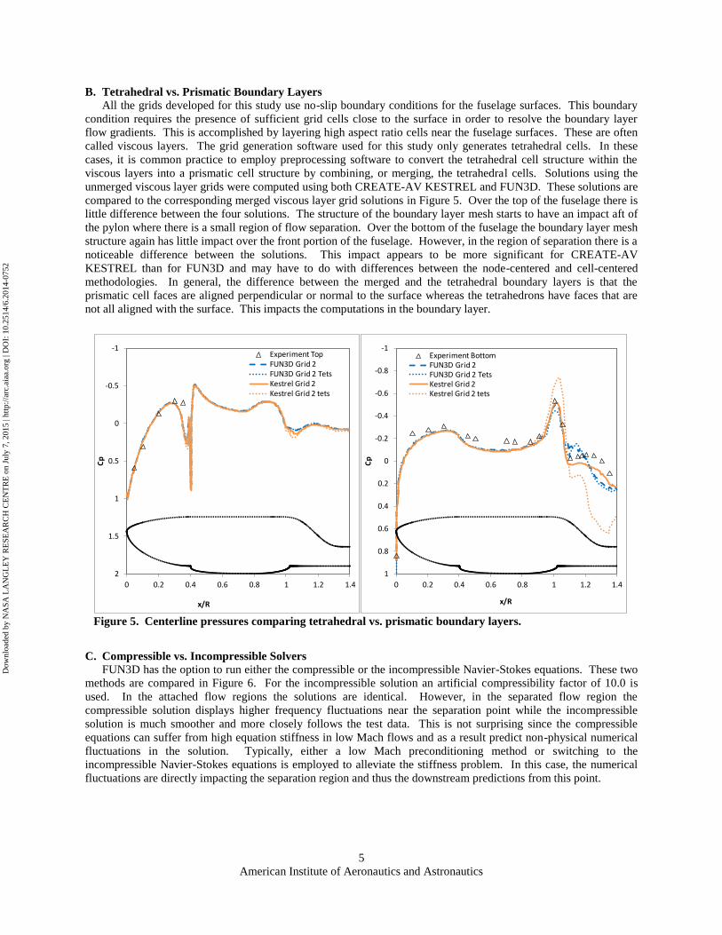
B. Tetrahedral vs. Prismatic Boundary Layers
All the grids developed for this study use no-slip boundary conditions for the fuselage surfaces. This boundary
condition requires the presence of sufficient grid cells close to the surface in order to resolve the boundary layer
flow gradients. This is accomplished by layering high aspect ratio cells near the fuselage surfaces. These are often
called viscous layers. The grid generation software used for this study only generates tetrahedral cells. In these
cases, it is common practice to employ preprocessing software to convert the tetrahedral cell structure within the
viscous layers into a prismatic cell structure by combining, or merging, the tetrahedral cells. Solutions using the
unmerged viscous layer grids were computed using both CREATE-AV KESTREL and FUN3D. These solutions are
compared to the corresponding merged viscous layer grid solutions in Figure 5. Over the top of the fuselage there is
little difference between the four solutions. The structure of the boundary layer mesh starts to have an impact aft of
the pylon where there is a small region of flow separation. Over the bottom of the fuselage the boundary layer mesh
structure again has little impact over the front portion of the fuselage. However, in the region of separation there is a
noticeable difference between the solutions. This impact appears to be more significant for CREATE-AV
KESTREL than for FUN3D and may have to do with differences between the node-centered and cell-centered
methodologies. In general, the difference between the merged and the tetrahedral boundary layers is that the
prismatic cell faces are aligned perpendicular or normal to the surface whereas the tetrahedrons have faces that are
not all aligned with the surface. This impacts the computations in the boundary layer.
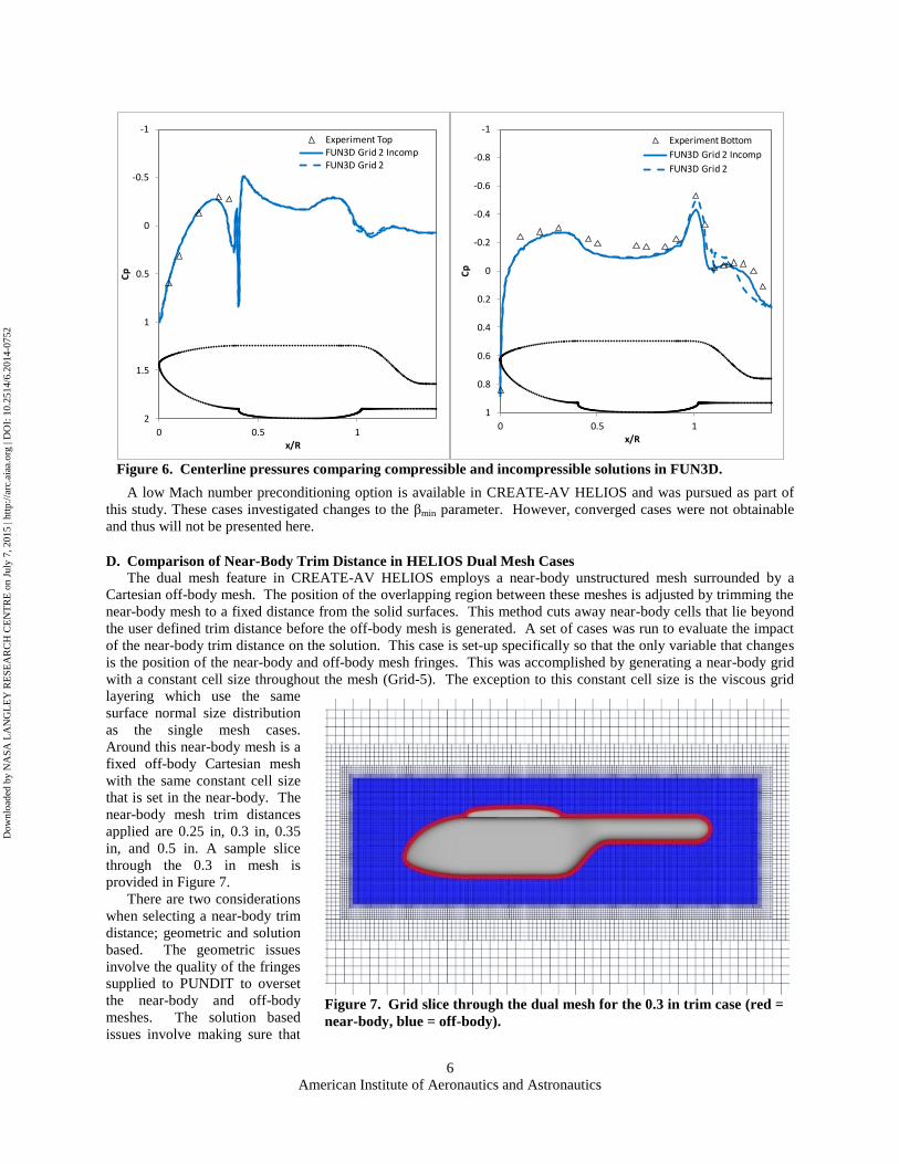
C. Compressible vs. Incompressible Solvers
FUN3D has the option to run either the compressible or the incompressible Navier-Stokes equations. These two
methods are compared in Figure 6. For the incompressible solution an artificial compressibility factor of 10.0 is
used. In the attached flow regions the solutions are identical. However, in the separated flow region the
compressible solution displays higher frequency fluctuations near the separation point while the incompressible
solution is much smoother and more closely follows the test data. This is not surprising since the compressible
equations can suffer from high equation stiffness in low Mach flows and as a result predict non-physical numerical
fluctuations in the solution. Typically, either a low Mach preconditioning method or switching to the
incompressible Navier-Stokes equations is employed to alleviate the stiffness problem. In this case, the numerical
fluctuations are directly impacting the separation region and thus the downstream predictions from this point.
-1
-0.5
0
0.5
1
1.5
2
0 0.2 0.4 0.6 0.8 1 1.2 1.4
Cp
x/R
Experiment TopFUN3D Grid 2FUN3D Grid 2 TetsKestrel Grid 2Kestrel Grid 2 tets
-1
-0.8
-0.6
-0.4
-0.2
0
0.2
0.4
0.6
0.8
1
0 0.2 0.4 0.6 0.8 1 1.2 1.4
Cp
x/R
Experiment BottomFUN3D Grid 2FUN3D Grid 2 TetsKestrel Grid 2Kestrel Grid 2 tets
Figure 5. Centerline pressures comparing tetrahedral vs. prismatic boundary layers.
Dow
nloa
ded
by N
ASA
LA
NG
LE
Y R
ESE
AR
CH
CE
NT
RE
on
July
7, 2
015
| http
://ar
c.ai
aa.o
rg |
DO
I: 1
0.25
14/6
.201
4-07
52
American Institute of Aeronautics and Astronautics
6
A low Mach number preconditioning option is available in CREATE-AV HELIOS and was pursued as part of
this study. These cases investigated changes to the βmin parameter. However, converged cases were not obtainable
and thus will not be presented here.
D. Comparison of Near-Body Trim Distance in HELIOS Dual Mesh Cases
The dual mesh feature in CREATE-AV HELIOS employs a near-body unstructured mesh surrounded by a
Cartesian off-body mesh. The position of the overlapping region between these meshes is adjusted by trimming the
near-body mesh to a fixed distance from the solid surfaces. This method cuts away near-body cells that lie beyond
the user defined trim distance before the off-body mesh is generated. A set of cases was run to evaluate the impact
of the near-body trim distance on the solution. This case is set-up specifically so that the only variable that changes
is the position of the near-body and off-body mesh fringes. This was accomplished by generating a near-body grid
with a constant cell size throughout the mesh (Grid-5). The exception to this constant cell size is the viscous grid
layering which use the same
surface normal size distribution
as the single mesh cases.
Around this near-body mesh is a
fixed off-body Cartesian mesh
with the same constant cell size
that is set in the near-body. The
near-body mesh trim distances
applied are 0.25 in, 0.3 in, 0.35
in, and 0.5 in. A sample slice
through the 0.3 in mesh is
provided in Figure 7.
There are two considerations
when selecting a near-body trim
distance; geometric and solution
based. The geometric issues
involve the quality of the fringes
supplied to PUNDIT to overset
the near-body and off-body
meshes. The solution based
issues involve making sure that
-1
-0.5
0
0.5
1
1.5
2
0 0.5 1
Cp
x/R
Experiment TopFUN3D Grid 2 IncompFUN3D Grid 2
-1
-0.8
-0.6
-0.4
-0.2
0
0.2
0.4
0.6
0.8
1
0 0.5 1
Cp
x/R
Experiment Bottom
FUN3D Grid 2 Incomp
FUN3D Grid 2
Figure 6. Centerline pressures comparing compressible and incompressible solutions in FUN3D.
Figure 7. Grid slice through the dual mesh for the 0.3 in trim case (red =
near-body, blue = off-body).
Dow
nloa
ded
by N
ASA
LA
NG
LE
Y R
ESE
AR
CH
CE
NT
RE
on
July
7, 2
015
| http
://ar
c.ai
aa.o
rg |
DO
I: 1
0.25
14/6
.201
4-07
52

American Institute of Aeronautics and Astronautics
7
-1
-0.5
0
0.5
1
1.5
2
0 0.2 0.4 0.6 0.8 1 1.2 1.4
Cp
x/R
Experiment TopHelios Grid 2 N/AHelios Grid 5 0.5Helios Grid 5 0.35Helios Grid 5 0.3
-1
-0.8
-0.6
-0.4
-0.2
0
0.2
0.4
0.6
0.8
1
0 0.2 0.4 0.6 0.8 1 1.2 1.4
Cp
x/R
Experiment BottomHelios Grid 2 N/AHelios Grid 5 0.5Helios Grid 5 0.35Helios Grid 5 0.3
Figure 9. Centerline pressures comparing near-body trim distance in Helios dual mesh cases.
the Euler off-body solution does not cover any regions where viscous effects are important. The consequences of
exceeding the geometric limit are best shown in the 0.25 in trim case. This case computed a total of 4515 orphans.
These orphans are illustrated in Figure 8 where the orphan locations are represented by the green spots. All of these
orphans are located in places where the off-body Cartesian mesh intersects the second viscous grid layer. In this
plot the black represents the off-body mesh, the red and blue represent the near-body mesh where the blue is the
near-body fringe. Therefore, the trim distance must be increased in order to move the off-body fringe away from the
viscous grid layers and thus reduce the number of orphans. The 0.3 in case has a total of 241 orphans. This is below
the default reject threshold of 1000 and was allowed to complete. The 0.35 in and the 0.5 in cases both compute
zero orphans.
The next step is to make sure that the Euler solution does not overlap the viscous regions. This is more difficult
to identify, but generally requires that the off-body not cut into the boundary layer. The centerline pressure
predictions for the 0.3 in, 0.35 in, and the 0.5 in trim cases are compared in Figure 9. It is apparent from this
comparison that the Euler assumptions in the off-body are interfering with the near-body predictions in the 0.3 in
case. This is further illustrated in Figure 10 where there is additional unsteadiness predicted around the attached
flow regions of the fuselage. The solutions for the 0.35 in and the 0.5 in cases are much smoother and predict the
same solution for the attached flow regions. Thus, in these regions the Euler off-body is not overlapping the
Figure 8. Orphan locations for the 0.25 in trim distance case.
Dow
nloa
ded
by N
ASA
LA
NG
LE
Y R
ESE
AR
CH
CE
NT
RE
on
July
7, 2
015
| http
://ar
c.ai
aa.o
rg |
DO
I: 1
0.25
14/6
.201
4-07
52

American Institute of Aeronautics and Astronautics
8
boundary layer for trim distances greater than 0.35 in.
In the separated flow region, the solutions begin to diverge. The single mesh case is included to show that as the
trim distance is increased the solution is trending towards the single mesh case. However, the equivalent single
mesh case would actually use a much finer grid than the Grid-2 case plotted here. There seems to be an optimum
point between 0.3 in and 0.35 in that would produce the closest solution. However, a solution dependent on trim
distance is not the ideal situation. The off-body mesh is intended to provide both efficiency and accuracy to the
solution through quicker per node computation time, increased spatial order of accuracy, and adaptive mesh
refinement. In this case, for which the mesh refinement is fixed, the variables that differ between the near-body and
the off-body are primarily the inviscid flow assumption and the increased spatial accuracy. The spatial accuracy
would certainly increase the resolution of the flow structures in the flow aft of the fuselage in the off-body region. It
may be that the increased spatial order of accuracy close to the surface is impacting the separation characteristics, or
it may be that the trim distance is not sufficiently large in the separated flow region so that the Euler flow
assumption is valid.
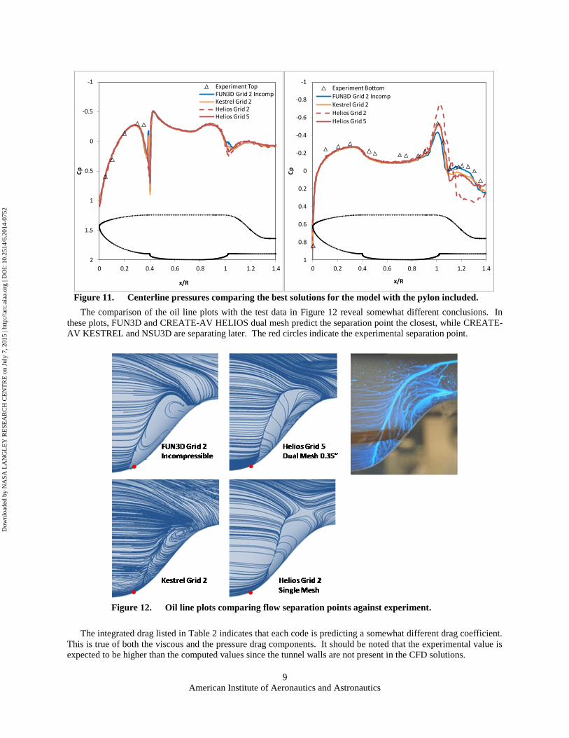
E. Initial Solver Comparison
This initial solver comparison looks specifically at comparing the best solutions obtained with each solver using
the geometry with the pylon included. For CREATE-AV KESTREL this is the Grid-2 merged boundary layer case,
for FUN3D this is the Grid-2 merged boundary layer incompressible case, and for CREATE-AV HELIOS this is the
Grid-5 combined NSU3D/ARC3D
solution with the additional off-
body refinement aft of the fuselage
and the 0.35 in trim distance. The
isolated NSU3D solution using
Grid-2 is included since it matches
the FUN3D and CREATE-AV
KESTREL conditions the closest.
These solutions are plotted in
Figure 11. For the attached flow
region the solutions are almost
identical, there is a small
divergence for the NSU3D solution
along the bottom of the fuselage.
In the separated flow regions each
code predicts a different solution.
The CREATE-AV HELIOS dual
mesh and CREATE-AV
KESTREL solutions seem to
predict the peak the best, while
FUN3D seems to predict the
separation point the best. The
isolated NSU3D solution has the
greatest error. It should be noted
that since the wind tunnel walls are
not modeled here that it is
unknown exactly how far off the
free air predictions should be from
the measured data. The next
section that compares the
OVERFLOW data with the current
predictions will approximate this
delta.
0.30”
0.35”
0.50”
Figure 10. Centerline slices comparing the velocity contours for
different near-body trim distances.
Dow
nloa
ded
by N
ASA
LA
NG
LE
Y R
ESE
AR
CH
CE
NT
RE
on
July
7, 2
015
| http
://ar
c.ai
aa.o
rg |
DO
I: 1
0.25
14/6
.201
4-07
52
American Institute of Aeronautics and Astronautics
9
The comparison of the oil line plots with the test data in Figure 12 reveal somewhat different conclusions. In
these plots, FUN3D and CREATE-AV HELIOS dual mesh predict the separation point the closest, while CREATE-
AV KESTREL and NSU3D are separating later. The red circles indicate the experimental separation point.
The integrated drag listed in Table 2 indicates that each code is predicting a somewhat different drag coefficient.
This is true of both the viscous and the pressure drag components. It should be noted that the experimental value is
expected to be higher than the computed values since the tunnel walls are not present in the CFD solutions.
Figure 12. Oil line plots comparing flow separation points against experiment.
-1
-0.5
0
0.5
1
1.5
2
0 0.2 0.4 0.6 0.8 1 1.2 1.4
Cp
x/R
Experiment TopFUN3D Grid 2 IncompKestrel Grid 2Helios Grid 2Helios Grid 5
-1
-0.8
-0.6
-0.4
-0.2
0
0.2
0.4
0.6
0.8
1
0 0.2 0.4 0.6 0.8 1 1.2 1.4
Cp
x/R
Experiment Bottom
FUN3D Grid 2 Incomp
Kestrel Grid 2Helios Grid 2
Helios Grid 5
Figure 11. Centerline pressures comparing the best solutions for the model with the pylon included.
Dow
nloa
ded
by N
ASA
LA
NG
LE
Y R
ESE
AR
CH
CE
NT
RE
on
July
7, 2
015
| http
://ar
c.ai
aa.o
rg |
DO
I: 1
0.25
14/6
.201
4-07
52
American Institute of Aeronautics and Astronautics
10
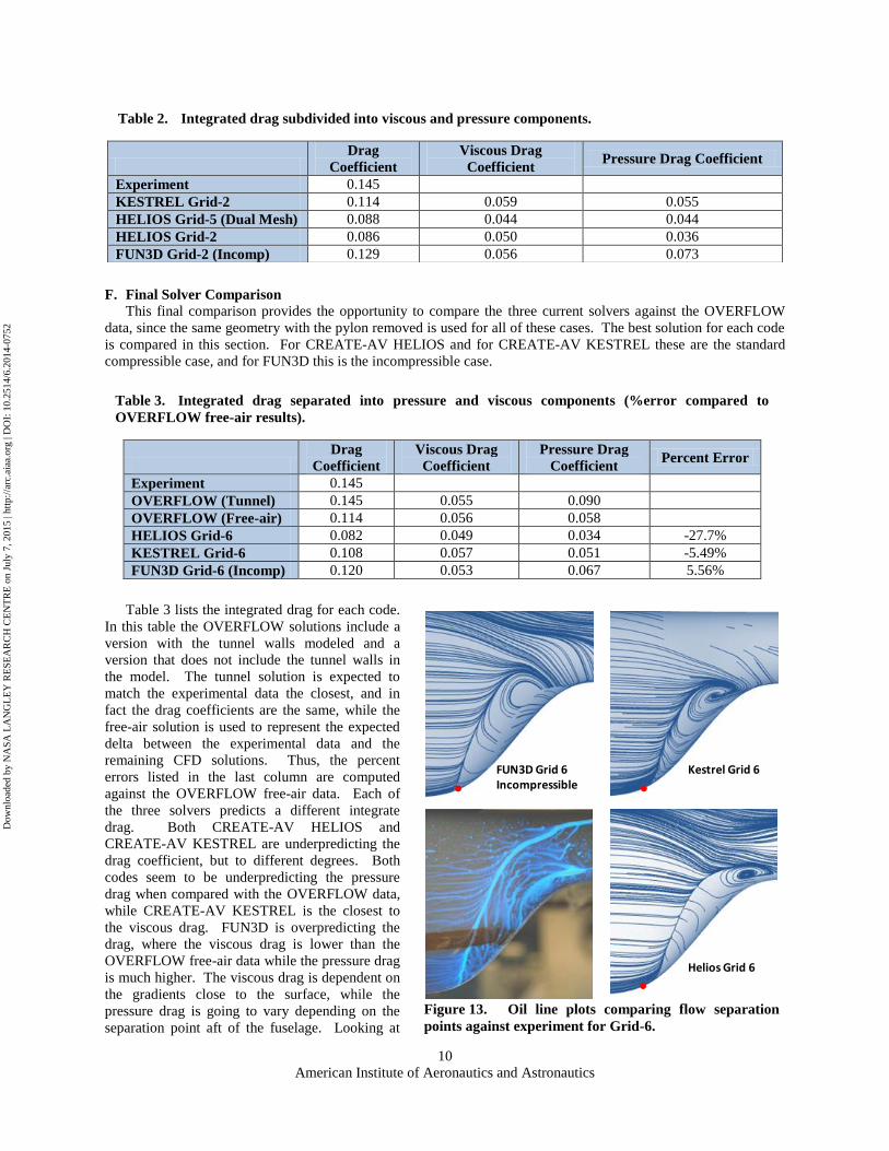
F. Final Solver Comparison
This final comparison provides the opportunity to compare the three current solvers against the OVERFLOW
data, since the same geometry with the pylon removed is used for all of these cases. The best solution for each code
is compared in this section. For CREATE-AV HELIOS and for CREATE-AV KESTREL these are the standard
compressible case, and for FUN3D this is the incompressible case.
Table 3 lists the integrated drag for each code.
In this table the OVERFLOW solutions include a
version with the tunnel walls modeled and a
version that does not include the tunnel walls in
the model. The tunnel solution is expected to
match the experimental data the closest, and in
fact the drag coefficients are the same, while the
free-air solution is used to represent the expected
delta between the experimental data and the
remaining CFD solutions. Thus, the percent
errors listed in the last column are computed
against the OVERFLOW free-air data. Each of
the three solvers predicts a different integrate
drag. Both CREATE-AV HELIOS and
CREATE-AV KESTREL are underpredicting the
drag coefficient, but to different degrees. Both
codes seem to be underpredicting the pressure
drag when compared with the OVERFLOW data,
while CREATE-AV KESTREL is the closest to
the viscous drag. FUN3D is overpredicting the
drag, where the viscous drag is lower than the
OVERFLOW free-air data while the pressure drag
is much higher. The viscous drag is dependent on
the gradients close to the surface, while the
pressure drag is going to vary depending on the
separation point aft of the fuselage. Looking at
Table 3. Integrated drag separated into pressure and viscous components (%error compared to
OVERFLOW free-air results).
Drag
Coefficient
Viscous Drag
Coefficient
Pressure Drag
Coefficient Percent Error
Experiment 0.145
OVERFLOW (Tunnel) 0.145 0.055 0.090
OVERFLOW (Free-air) 0.114 0.056 0.058
HELIOS Grid-6 0.082 0.049 0.034 -27.7%
KESTREL Grid-6 0.108 0.057 0.051 -5.49%
FUN3D Grid-6 (Incomp) 0.120 0.053 0.067 5.56%
Table 2. Integrated drag subdivided into viscous and pressure components.
Drag
Coefficient
Viscous Drag
Coefficient Pressure Drag Coefficient
Experiment 0.145
KESTREL Grid-2 0.114 0.059 0.055
HELIOS Grid-5 (Dual Mesh) 0.088 0.044 0.044
HELIOS Grid-2 0.086 0.050 0.036
FUN3D Grid-2 (Incomp) 0.129 0.056 0.073
FUN3D Grid 6Incompressible
Kestrel Grid 6
Helios Grid 6
Figure 13. Oil line plots comparing flow separation
points against experiment for Grid-6.
Dow
nloa
ded
by N
ASA
LA
NG
LE
Y R
ESE
AR
CH
CE
NT
RE
on
July
7, 2
015
| http
://ar
c.ai
aa.o
rg |
DO
I: 1
0.25
14/6
.201
4-07
52
American Institute of Aeronautics and Astronautics
11
FUN3D Grid 6 Incompressible
Helios Grid 6
Kestrel Grid 6
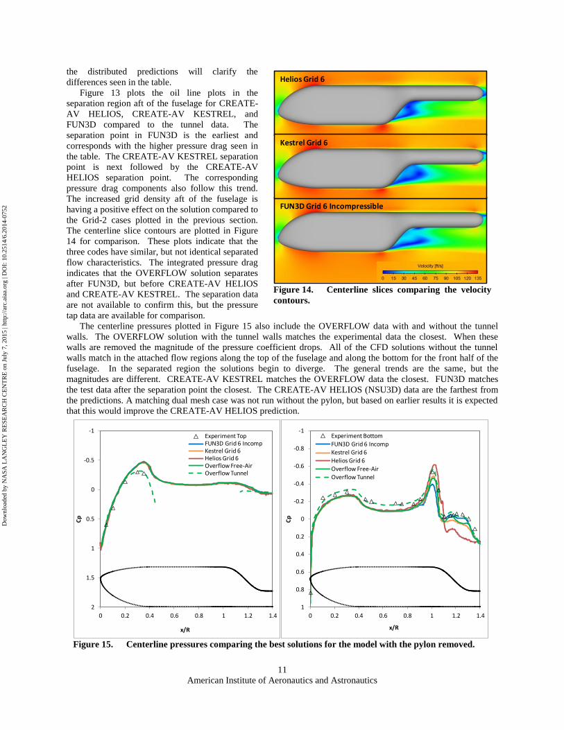
Figure 14. Centerline slices comparing the velocity
contours.
the distributed predictions will clarify the
differences seen in the table.
Figure 13 plots the oil line plots in the
separation region aft of the fuselage for CREATE-
AV HELIOS, CREATE-AV KESTREL, and
FUN3D compared to the tunnel data. The
separation point in FUN3D is the earliest and
corresponds with the higher pressure drag seen in
the table. The CREATE-AV KESTREL separation
point is next followed by the CREATE-AV
HELIOS separation point. The corresponding
pressure drag components also follow this trend.
The increased grid density aft of the fuselage is
having a positive effect on the solution compared to
the Grid-2 cases plotted in the previous section.
The centerline slice contours are plotted in Figure
14 for comparison. These plots indicate that the
three codes have similar, but not identical separated
flow characteristics. The integrated pressure drag
indicates that the OVERFLOW solution separates
after FUN3D, but before CREATE-AV HELIOS
and CREATE-AV KESTREL. The separation data
are not available to confirm this, but the pressure
tap data are available for comparison.
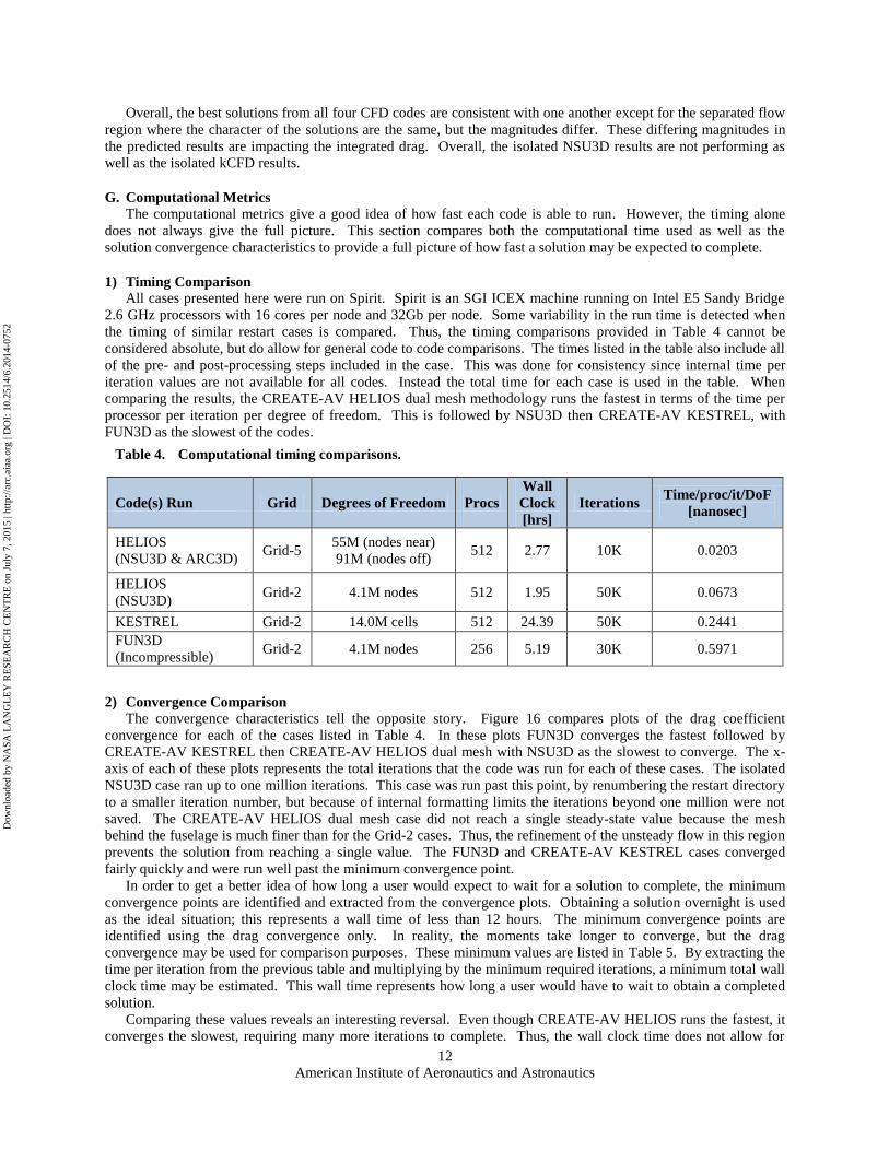
The centerline pressures plotted in Figure 15 also include the OVERFLOW data with and without the tunnel
walls. The OVERFLOW solution with the tunnel walls matches the experimental data the closest. When these
walls are removed the magnitude of the pressure coefficient drops. All of the CFD solutions without the tunnel
walls match in the attached flow regions along the top of the fuselage and along the bottom for the front half of the
fuselage. In the separated region the solutions begin to diverge. The general trends are the same, but the
magnitudes are different. CREATE-AV KESTREL matches the OVERFLOW data the closest. FUN3D matches
the test data after the separation point the closest. The CREATE-AV HELIOS (NSU3D) data are the farthest from
the predictions. A matching dual mesh case was not run without the pylon, but based on earlier results it is expected
that this would improve the CREATE-AV HELIOS prediction.
-1
-0.5
0
0.5
1
1.5
2
0 0.2 0.4 0.6 0.8 1 1.2 1.4
Cp
x/R
Experiment TopFUN3D Grid 6 IncompKestrel Grid 6Helios Grid 6Overflow Free-AirOverflow Tunnel
-1
-0.8
-0.6
-0.4
-0.2
0
0.2
0.4
0.6
0.8
1
0 0.2 0.4 0.6 0.8 1 1.2 1.4
Cp
x/R
Experiment Bottom
FUN3D Grid 6 Incomp
Kestrel Grid 6
Helios Grid 6
Overflow Free-Air
Overflow Tunnel
Figure 15. Centerline pressures comparing the best solutions for the model with the pylon removed.
Dow
nloa
ded
by N
ASA
LA
NG
LE
Y R
ESE
AR
CH
CE
NT
RE
on
July
7, 2
015
| http
://ar
c.ai
aa.o
rg |
DO
I: 1
0.25
14/6
.201
4-07
52
American Institute of Aeronautics and Astronautics
12
Overall, the best solutions from all four CFD codes are consistent with one another except for the separated flow
region where the character of the solutions are the same, but the magnitudes differ. These differing magnitudes in
the predicted results are impacting the integrated drag. Overall, the isolated NSU3D results are not performing as
well as the isolated kCFD results.
G. Computational Metrics
The computational metrics give a good idea of how fast each code is able to run. However, the timing alone
does not always give the full picture. This section compares both the computational time used as well as the
solution convergence characteristics to provide a full picture of how fast a solution may be expected to complete.
1) Timing Comparison
All cases presented here were run on Spirit. Spirit is an SGI ICEX machine running on Intel E5 Sandy Bridge
2.6 GHz processors with 16 cores per node and 32Gb per node. Some variability in the run time is detected when
the timing of similar restart cases is compared. Thus, the timing comparisons provided in Table 4 cannot be
considered absolute, but do allow for general code to code comparisons. The times listed in the table also include all
of the pre- and post-processing steps included in the case. This was done for consistency since internal time per
iteration values are not available for all codes. Instead the total time for each case is used in the table. When
comparing the results, the CREATE-AV HELIOS dual mesh methodology runs the fastest in terms of the time per
processor per iteration per degree of freedom. This is followed by NSU3D then CREATE-AV KESTREL, with
FUN3D as the slowest of the codes.
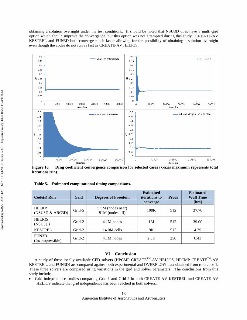
2) Convergence Comparison
The convergence characteristics tell the opposite story. Figure 16 compares plots of the drag coefficient
convergence for each of the cases listed in Table 4. In these plots FUN3D converges the fastest followed by
CREATE-AV KESTREL then CREATE-AV HELIOS dual mesh with NSU3D as the slowest to converge. The x-
axis of each of these plots represents the total iterations that the code was run for each of these cases. The isolated
NSU3D case ran up to one million iterations. This case was run past this point, by renumbering the restart directory
to a smaller iteration number, but because of internal formatting limits the iterations beyond one million were not
saved. The CREATE-AV HELIOS dual mesh case did not reach a single steady-state value because the mesh
behind the fuselage is much finer than for the Grid-2 cases. Thus, the refinement of the unsteady flow in this region
prevents the solution from reaching a single value. The FUN3D and CREATE-AV KESTREL cases converged
fairly quickly and were run well past the minimum convergence point.
In order to get a better idea of how long a user would expect to wait for a solution to complete, the minimum
convergence points are identified and extracted from the convergence plots. Obtaining a solution overnight is used
as the ideal situation; this represents a wall time of less than 12 hours. The minimum convergence points are
identified using the drag convergence only. In reality, the moments take longer to converge, but the drag
convergence may be used for comparison purposes. These minimum values are listed in Table 5. By extracting the
time per iteration from the previous table and multiplying by the minimum required iterations, a minimum total wall
clock time may be estimated. This wall time represents how long a user would have to wait to obtain a completed
solution.
Comparing these values reveals an interesting reversal. Even though CREATE-AV HELIOS runs the fastest, it
converges the slowest, requiring many more iterations to complete. Thus, the wall clock time does not allow for
Table 4. Computational timing comparisons.
Code(s) Run Grid Degrees of Freedom Procs
Wall
Clock
[hrs]
Iterations Time/proc/it/DoF
[nanosec]
HELIOS
(NSU3D & ARC3D) Grid-5
55M (nodes near)
91M (nodes off) 512 2.77 10K 0.0203
HELIOS
(NSU3D) Grid-2 4.1M nodes 512 1.95 50K 0.0673
KESTREL Grid-2 14.0M cells 512 24.39 50K 0.2441
FUN3D
(Incompressible) Grid-2 4.1M nodes 256 5.19 30K 0.5971
Dow
nloa
ded
by N
ASA
LA
NG
LE
Y R
ESE
AR
CH
CE
NT
RE
on
July
7, 2
015
| http
://ar
c.ai
aa.o
rg |
DO
I: 1
0.25
14/6
.201
4-07
52
American Institute of Aeronautics and Astronautics
13
obtaining a solution overnight under the test conditions. It should be noted that NSU3D does have a multi-grid
option which should improve the convergence, but this option was not attempted during this study. CREATE-AV
KESTREL and FUN3D both converge much faster allowing for the possibility of obtaining a solution overnight
even though the codes do not run as fast as CREATE-AV HELIOS.
VI. Conclusion
A study of three locally available CFD solvers (HPCMP CREATETM
-AV HELIOS, HPCMP CREATETM
-AV
KESTREL, and FUN3D) are compared against both experimental and OVERFLOW data obtained from reference 1.
These three solvers are compared using variations in the grid and solver parameters. The conclusions from this
study include,
Grid independence studies comparing Grid-1 and Grid-2 in both CREATE-AV KESTREL and CREATE-AV
HELIOS indicate that grid independence has been reached in both solvers.
Table 5. Estimated computational timing comparisons.
Code(s) Run Grid Degrees of Freedom
Estimated
iterations to
converge
Procs
Estimated
Wall Time
[hrs]
HELIOS
(NSU3D & ARC3D) Grid-5
5.5M (nodes near)
91M (nodes off) 100K 512 27.70
HELIOS
(NSU3D) Grid-2 4.1M nodes 1M 512 39.00
KESTREL Grid-2 14.0M cells 9K 512 4.39
FUN3D
(Incompressible) Grid-2 4.1M nodes 2.5K 256 0.43
Figure 16. Drag coefficient convergence comparison for selected cases (x-axis maximum represents total
iterations run).
Dow
nloa
ded
by N
ASA
LA
NG
LE
Y R
ESE
AR
CH
CE
NT
RE
on
July
7, 2
015
| http
://ar
c.ai
aa.o
rg |
DO
I: 1
0.25
14/6
.201
4-07
52
American Institute of Aeronautics and Astronautics
14
The comparison of tetrahedral vs. prismatic boundary layers indicates that the surface aligned faces in the
prismatic boundary layer yield better results than the unaligned faces in the tetrahedral boundary layer. This
difference is stronger in the cell-centered CREATE-AV KESTREL code than in the node-centered FUN3D
code.
The use of the incompressible equations reduces the incidence of non-physical numerical fluctuation in the
FUN3D solution.
When setting up a dual mesh case in CREATE-AV HELIOS care must be taken when defining the fringe
distance to both create a proper fringe for the oversetting process, as well as to keep sufficient distance of the
off-body solver from the viscous flow regions.
The initial comparison with the pylon included indicate that in the attached flow regions all of the solutions
predict approximately the same results. The separated regions predict different magnitude solutions with the
isolated NSU3D solution being the furthest from the experimental data.
The final comparison with the pylon removed allows for the comparison with the OVERFLOW data. In this
comparison all of the local CFD solvers predicted the drag to be within 6% error with the exception of the
CREATE-AV HELIOS prediction. The distributed data showed that the differences are primarily in the
separated flow aft of the fuselage.
The computational metrics show that CREATE-AV HELIOS runs the fastest and CREATE-AV KESTREL and
FUN3D run the slowest. However, the increased rate of convergence in CREATE-AV KESTREL and FUN3D
allow for a solution to be obtained overnight, while more time is needed for a CREATE-AV HELIOS solution.
Finally, it should be pointed out that this study did not do a thorough investigation of optimal solver settings,
default settings in the solvers were used in most cases, only a few deviations from these settings were attempted.
Since HELIOS is applied primarily to rotor-based flows, as opposed to isolated fuselages like the fixed-wing kCFD
code, the default settings in HELIOS may not have been ideal for this fuselage case. Future work will investigate
alternative solver settings in HELIOS in order to see if the results improve.
Acknowledgments
The authors would like to acknowledge the support of the HPCMP CREATETM
-AV Program and the
supercomputing resources provided by the HPCMP, in particular the Air Force Research Lab (AFRL). The
contribution of Rajneesh Singh of providing the original ROBIN surface mesh is also gratefully acknowledged.
References
1Schaeffler, N. W., Allan, B. G., Lienard, C., and Le Pape, A., “Progress Towards Fuselage Drag Reduction via
Active Flow Control: A Combined CFD and Experimental Effort,” 36th
European Rotorcraft Forum, Paris, France,
September 7-9, 2010.
2Singh, R., and Dinavahi, S., “Aerodynamic Force Computations for Rotorcraft Fuselage,” 50
th AIAA Aerospace
Sciences Meeting, Nashville, TN, January 9-12, 2012.
3HPCMP CREATE
TM-AV On-line Resources, “https://portal.create.hpc.mil/authdocs/av/index.php,” Last Accessed
November 18th
, 2013.
4FUN3D On-line Resources, “http://fun3d.larc.nasa.gov,” Last Accessed November 18
th, 2013.
Dow
nloa
ded
by N
ASA
LA
NG
LE
Y R
ESE
AR
CH
CE
NT
RE
on
July
7, 2
015
| http
://ar
c.ai
aa.o
rg |
DO
I: 1
0.25
14/6
.201
4-07
52
Recommended