Chaotic dynamics of a behavior-based miniature mobile robot:
effects of environment and control structure
Md. Monirul Islama, K. Muraseb,*
aDepartment of Computer Science and Engineering, Bangladesh University of Engineering and Technology (BUET), Dhaka 1000, BangladeshbDepartment of Human and Artificial Intelligence Systems (HART), University of Fukui, 3-9-1 Bunkyo, Fukui 910-8507, Japan
Received 9 January 2002; revised 14 September 2004; accepted 14 September 2004
Abstract
To study the regularity and complexity of autonomous behavior, the flow of sensory information obtained in autonomous mobile robots
under various conditions was analyzed as a complex system. Sensory information time series Xn was collected from a miniature mobile robot
during free navigation, and plotted on the return map, the graph of XnCt vs. Xn. The plot exhibited a characteristic trajectory, representing the
regularity of the time series. Correlation integral and Lyapunov exponent analysis also showed properties of deterministic chaos; the
presence of fractal dimension and positive Lyapunov exponent. Analysis of sensory information obtained in the robot with three different
neural controllers revealed that the autonomous robot behaves in such a way that the flow of sensory information is governed by a
deterministic rule, and this pattern is unique to each controller. Furthermore, the analysis in various environments exhibited that transitions
from one trajectory to another on the return map occur during the course of autonomous behavior. The fractal and Lyapunov dimensions
calculated in various conditions indicate that these dimension could be utilized to quantify the complexity of autonomous behavior and the
relative difficulty of tasks. Analyses at different evolutionary stage revealed that behavioral performance correlates with fractal dimension.
These studies using a miniature mobile robot that allowed to idealize the experimental conditions demonstrated firmly that the complex
analysis could be utilized in evaluation and optimization of autonomous systems and the behavior.
q 2004 Elsevier Ltd. All rights reserved.
Keywords: Chaos; Behavior-based robot; Mobile robot; Performance measure of robot; Self-organization
1. Introduction
The sensory information perceived by an autonomous
robot, as well as by living creatures, reflects dynamic
interactions between the robot and the environment in which
the robot is situated (Biro & Ziemke, 1998; Brooks, 1991;
Degn, Holden, & Olsen, 1997; Pfeiffer, 1995, Pfeiffer &
Scheier, 1997). Even in a static environment, the sensory
information received through sensory organs is dynamic
because of the behavior of the robot itself. In the behavior-
based robotics (Brooks, 1986, 1991), motor control signals
are generated by the flow of sensory information, which is
a function of the robot’s own behavior. Therefore,
during autonomous behavior, which is goal-directed
0893-6080/$ - see front matter q 2004 Elsevier Ltd. All rights reserved.
doi:10.1016/j.neunet.2004.09.002
* Corresponding author. Tel.: C81 776 27 8774; fax: C81 776 27 8420.
E-mail address: [email protected] (K. Murase).
and/or self-organized, the sensory information flow should
have an organization, or a hidden regularity (Odagiri,
Monirul Islam, Okura, Asai, & Murase, 1999; Odagiri, Wei,
Asai, & Murase, 1998a; Odagiri, Wei, Asai, Yamakawa, &
Murase, 1998b; Ziemke, 1996a,b). That is, although
fluctuation in the time series of sensory signals looks as if
random, there should exist a hidden regularity underlying it.
Although, the internal representation generating organized
behavior of the autonomous robot has been the target of
intensive research (e.g. Pfeiffer, 1995; Pfeiffer & Scheier,
1997) and the robot’s internal states have been investigated
(e.g. Ziemke, 1996a,b, 1998), further understanding of the
hidden regularity in their behavior as well as that of internal
states is needed.
The phenomenon that appears random but is regulated
under a deterministic rule is called deterministic chaos, and
its nature can be analyzed mathematically (Holden, 1986;
Jackson, 1989; Parker & Chua, 1987). Chaos has been found
Neural Networks 18 (2005) 123–144
www.elsevier.com/locate/neunet

Md. Monirul Islam, K. Murase / Neural Networks 18 (2005) 123–144124
in living organs such as in brain activity (Babloyantz,
Salazar, & Nicolis, 1985; Babloyantz & Destexhe, 1986),
neurons (Hayashi, Ishizuka, & Nicolis; 1985) and axons
(Matsumoto, Aihara, Hanyu, Takahashi, Yoshizawa, &
Nagumo, 1987), as well as artificial neural networks (Aihara,
Aihara, Takabe, & Toyota, 1990; Ikeguchi, Aihara, Ito, &
Utsunomiya, 1990) and others (Degn et al., 1997; Ott, 1993).
In the brain, spontaneous neuronal activity exhibits some
properties of deterministic chaos, and an alteration in its
profile occurs when a change in sensory information takes
place (Degn et al., 1997; Freeman, 1991, 1994a). It has been
thus considered that this chaos and transition might be the
underlying concept of perception and goal-directed, orga-
nized behavior (Freeman, 1994b; Kay, Lancaster, & Free-
man, 1996).
The regularity in the sensory information during
autonomous behavior is also found in artificial life. In an
autonomous mobile robot, the time series of sensory data
obtained during free navigation exhibits regularity on a
phase-plane plot called the return map (Smithers, 1995). It
has a fractal dimension of non-integer value, an important
property of deterministic chaos (Holden, 1986; Lorenz,
1994; Ott, 1993; Parker, & Chua, 1987). It is even suggested
that the regularity could be used as a performance measure
of autonomous robots. However, it is yet to be shown how
the regularity of a robot is altered when its environment
changes, and how it differs among robots with various
controllers. In such analysis, it is necessary to collect
sensory data sets of long period during free navigation of
robots in various conditions and it has been difficult to
perform the reliable experiments.
The purpose of this study is thus two folds. Firstly, we
intended to reveal whether or not phenomena similar to that
which takes place in the brain also takes place in artificial
life. We used a miniature autonomous mobile robot suitable
for rigorous, reproducible experiments. We obtained results
showing that the time series of sensory information obtained
during free navigation exhibits regularity, and that it has the
nature of deterministic chaos. We also investigated whether
or not the regularity changes in accordance with the
environmental alterations.
Secondly, we tried to reveal how the regularity differs
among individuals. This is essential for understanding the
nature of autonomy, as well as for testing whether or not it can
be utilized in practice as a performance measure of
autonomous robots. A given task could be difficult for a
particular robot but not for the others depending upon their
controlscheme,andthequantificationofthehardnessishighly
desirable.Wethusinvestigatedhowtheregularityvarieswhen
various neural controllers were loaded in the robot and
compared the regularity and performance among them.
This paper consists of five sections. In Section 2, we
describe the robot we used, and the way we collected and
constructed sensory information. In Section 3, methods and
results of analysis with the return map, the correlation
integral, Lyapunov exponent and the relation with
behavioral performance we used are described. In Section
4, we discuss the analyzed data in terms of individual
differences of regularity, the effect of environment on
regularity, transition of autonomous behavior, and the
fractal dimensions. Section 5 is Summary and Conclusion.
2. Experiments
This section describes the three types of autonomous
mobile robots used in this study, and the collection of the
sensory information during free movement in four different
environments. Three types of robots were modeled by three
different controllers loaded in a miniature mobile robot. In
order to perform reliable analysis, it is necessary to obtain
sensory time series of long duration with minimal noise. We
therefore, utilized a miniature mobile robot. It allowed long-
term recordings on a desk-top environment where external
noise could be maintained minimal. The robot was designed
as simple as possible, just sufficient to perform the desired
task. We used a simple neural network as a controller with
the minimal number of sensors, so that the results of
analysis became clear enough to exhibit the essence of
findings. Genetic evolution was used to determine the
parameters of the robot controllers so that the robot was
optimized for a given environment. Sensory information
time series were collected in four environments including
the evolved one for the analysis described in Section 3.
2.1. Experiments with three types of autonomous
mobile robots
Three types of robots were constructed by loading
different neural networks into a miniature mobile robot. The
neural network was intended to produce motor control
signals based on the proximity sensor signals. The
connection weights of each neural network were determined
by the genetic evolution for navigation and obstacle
avoidance in a field called the Maze environment.
2.1.1. Miniature mobile robot
We used a real mobile robot Khepera, whose structure
and function have been well described elsewhere (Mondada,
Franzi, & Ienne 1993). In short, its size is small: 55 cm in
diameter, 30 mm in height, and 70 g in weight. It consists of
two boards: the CPU board and the sensory-motor board.
The CPU board contains a microprocessor (Motorola
MC68311) with 128 Kbytes of EEPROM and 256 Kbytes
of static RAM, an A/D converter for the acquisition of
analogue signals coming from the sensory-motor board, a
proportional-integral–differential (PID) controller for the
motor control, and a RS232C serial port together
with power-supply terminals which is used for data
transmission to and from an external computer system and
for providing electricity from an external power-supply unit.
The microprocessor can execute programs downloaded
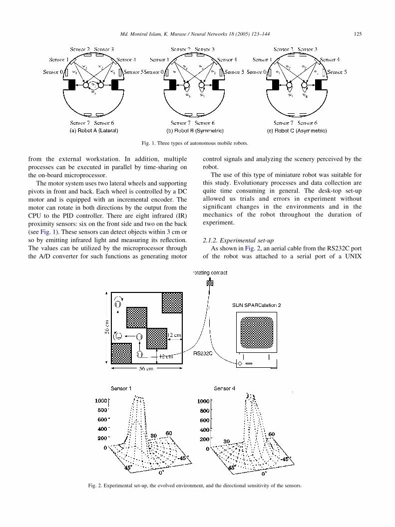
Fig. 1. Three types of autonomous mobile robots.
Md. Monirul Islam, K. Murase / Neural Networks 18 (2005) 123–144 125
from the external workstation. In addition, multiple
processes can be executed in parallel by time-sharing on
the on-board microprocessor.
The motor system uses two lateral wheels and supporting
pivots in front and back. Each wheel is controlled by a DC
motor and is equipped with an incremental encoder. The
motor can rotate in both directions by the output from the
CPU to the PID controller. There are eight infrared (IR)
proximity sensors: six on the front side and two on the back
(see Fig. 1). These sensors can detect objects within 3 cm or
so by emitting infrared light and measuring its reflection.
The values can be utilized by the microprocessor through
the A/D converter for such functions as generating motor
Fig. 2. Experimental set-up, the evolved environmen
control signals and analyzing the scenery perceived by the
robot.
The use of this type of miniature robot was suitable for
this study. Evolutionary processes and data collection are
quite time consuming in general. The desk-top set-up
allowed us trials and errors in experiment without
significant changes in the environments and in the
mechanics of the robot throughout the duration of
experiment.
2.1.2. Experimental set-up
As shown in Fig. 2, an aerial cable from the RS232C port
of the robot was attached to a serial port of a UNIX
t, and the directional sensitivity of the sensors.

Md. Monirul Islam, K. Murase / Neural Networks 18 (2005) 123–144126
workstation SUN SPARCstation 2 via a miniature rotating
contact. The generation of autonomous behavior by
calculating motor outputs from sensor readings, and
monitoring and storing sensor, motor and encoder values
were performed by the on-board microprocessor and
memory, while other processes such as constructing neural
networks, executing genetic operations, and detailed
analysis of sensory signals were managed by the external
workstation.
2.1.3. Three types of robots
Fig. 1 shows the three types of two-layered neural
networks loaded on the on-board microprocessor to produce
motor control signals from sensor signals. These robots with
different neural networks were designated as robots A, B,
and C. The neural networks of robots A, B, and C were
characterized by the presence of lateral connections,
symmetric recurrent connections, and asymmetric recurrent
connections, respectively. The connection weights were
symmetric except for the asymmetric recurrent connection
of robot C. There existed, so to speak, a structural difference
of the network between robot B and C, and a topological
difference in robot C to robots A and B.
Unlike most of the previous works regarding obstacle
avoidance (e.g. Floreano & Mondada, 1994, 1996; Naito,
Odagiri, Matsunaga, Tanifuji, & Murase, 1997; Nolfi,
Floreano, Miglino, & Mondada, 1994), the input signals
coming from only two front sensors, 1 and 4, were fed to the
neural network. It has been reported that two front sensors
are sufficient for navigation in simple environments such as
that shown in Fig. 2, and the use of two sensors simplifies
the following analysis of the sensory information as well
(Odagiri et al., 1998a,b). The sights of both sensors
illustrated are in Fig. 2. The robot was placed at the center
of circles, and the sensor readings were measured when a
white paper wall was placed at various positions against the
robot. The sensor could detect the wall within 60 mm from
the center of the robot or 37.5 mm away from each sensor.
Since the sensor value increased sharply from near zero to
near maximum for the wall at 30–20 mm from the sensor, a
several mm change in the distance within this range could
produce a large change in the sensor value on an order of
several hundred. Each sensor covered approximately 90
degrees of the field, and thus by using both sensors 1 and 4,
the wall located in the entire front area of the robot could be
detected.
Each output of the neural network was produced as a
weighted sum of two sensor signals and one lateral or
recurrent input as follows
Sp Z Sb CGX
wixi (1)
where Sp, Sb, G, wi, and xi represent the output for the motor,
the base navigation speed of the motor, the global gain, the
connection weights from sensors and output cell, and the
signals from corresponding sensors and output cell,
respectively. The values for Sb and G were set to 5 cm/s
and 1/800, respectively.
2.1.4. Genetic evolution
For each of the robots, A, B, and C, a simple genetic
algorithm (Holland, 1975) was used to determine the values
of connection weights in the neural network The robots
were evolved in the field called the Maze environment
shown in Fig. 2. Each individual in a population had the
same constant length of chromosome corresponding to the
number of connections in the neural network. Each weight
was encoded on a gene of five bits. The first bit determined
the sign of the weight and the remaining four bits its
strength. The length of a chromosome thus became 15 bits
in robots A and B, and 20 bits in robot C.
Each chromosome corresponding to an individual in a
population was generated by the external workstation, and
loaded down to the on-board microprocessor. After decod-
ing into the corresponding neural network, the robot was
allowed to move in the environment shown in Fig. 2 with the
neural network’s input and output values as well as encoder
values sampled every 0.1 s. These values were then up-
loaded to the workstation for fitness evaluation. Between
individuals, the robot changed its position randomly by
Braitenberg algorithm (Braitenberg, 1984) in order to avoid
the effect of the previous individual’s action. This procedure
was repeated for all individuals. When all individuals had
been tested, three genetic operators-selective reproduction,
crossover, and mutation-were applied to create a completely
new population of the same size. The fitness function F used
to evaluate each individual in a population was expressed as
follows
F Z Dð1 KvÞð1 KsÞ (2)
Here D, v, and s were the normalized values of the total
mileage of both motors, the difference mileage between the
two motors, and the total of two sensor values, respectively,
which were acquired every 0.1 s for an individual life-time
period of 5 s. The fitness function has been a standard for
developing the obstacle-avoidance and navigation capa-
bility (e.g. Floreano & Mondada, 1994, 1996; Nolfi et al.,
1994). One population of 10 individuals was evolved for 50
generations of each robot. The cross-over rate, the mutation
rate, and the elite preservation rate in the roulette selection
used in the genetic operation were 0.7, 0.02, and 0.5,
respectively.
Fig. 3 shows examples of the evolution processes for
robots A, B, and C. Some individuals who faced against
walls with slipping wheels got high scores at the initial stage
of evolution, but the behavior improved steadily after
generations. Due to the short length of chromosomes, the
robots learned to navigate and avoid obstacles very quickly,
often within 30 generations. The best individuals in
generations 35–50, having fitness scores of 0.12–0.2,
could navigate the whole environment very smoothly.

Fig. 3. Evolution processes of three robots.
Md. Monirul Islam, K. Murase / Neural Networks 18 (2005) 123–144 127
They never bumped into walls and corners, and rather
maintained a straight trajectory when possible. Connection
weights of the best individuals were as follows: For
Robot A, w1ZC8, w2ZK14, and w3ZC9. For Robot B
w1ZC4, w2ZK12, and w3ZC11. For robot C, w1ZC4,
w2ZK16, w3ZC5, and w4ZC12. We used these best
individuals throughout the following studies.
Through visual observation of behavior, distinguishing
the three robots from each other was very difficult. This was
evidenced by the sensory information obtained in the Maze
environment as shown in Fig. 4. Sensory signals exhibited
periodical peaks in a similar manner in all three robots, but
the magnitudes varied among them. This indicates that all of
them rotated in the path of the field very well, but the
distance from the walls, especially at the corners, varied
among them by several millimeters.
2.2. Sensory information in four different environments
Each of the best robots A, B, and C obtained by genetic
evolution was placed in four different fields called the Maze,
Square, Dynamic, and the Straight-Corridor environments.
During free navigation in each environment, the proximity
sensor values of a robot were continuously sampled.
Using the sampled sensory signal, a time series representing
the proximity of the robot to the front obstacle, which we
call sensory information, was constructed. For each robot,
Fig. 4. Examples of signals det
four time series, each for one environment, were con-
structed. Thus, a total of twelve time series were constructed
for three robots in this study.
2.2.1. Environments
The four environments in which sensory information was
collected are shown in Fig. 5. White non-glossy card board
was pasted on straight wooden bars and they were used to
make the walls of the path and obstacles in the field. The Maze
environment was identical to the one wherein robots evolved.
Notice that the Maze environment consisted of straight paths
and right-angled corners. The Square environment also
consisted of straight paths of the same width and right-angled
corners as those of the Maze environment, but contained only
one-directional turns. In the Dynamic environment, an
obstacle was placed manually at 6–8 cm in front of the robot
navigating. The robot had to turn to avoid a head-on collision,
and after turning the robot again faced another obstacle in front
placed manually. This was repeated during its entire life. The
Straight-Corridor environment had the same width as the
straight paths of the Maze and Square environments. The robot
was placed in the field to go along the path, but not to face the
wall. The path was sufficiently long to allow the sensory
information to be collected for approximately 20 s because the
robot’s navigation speed was about 5 cm/s.
In order to avoid environmental noise, a number of
precautions were taken in this study. Experiments were done
ected by sensors 1 and 4.
Fig. 5. Tested environments.
Md. Monirul Islam, K. Murase / Neural Networks 18 (2005) 123–144128
in complete darkness. Records of sensor signals were taken
mostly in the late night in order to avoid unexpected exposure
of light during the course of recording. As apparent from
Fig. 2, the proximity sensors generated output signals when
the obstacles were within 3 cm or so. Any obstacles away
from it, or any movements occurred far from it were unlikely
to produce any signal. Therefore, the output of the sensors
contained only the information from walls and/or obstacles
within c.a. 3 cm with minimal noise from environment.
2.2.2. Proximity of the robot to the front obstacle
For each robot, the values of sensors 1 and 4 were
continuously sampled every 0.1 for 3072 s during free
navigation in the Square, Maze, and Dynamic environ-
ments, and Straight-Corridor environment. Since the size of
on-board memory of the robot was limited, it was not
possible to take 30720 (i.e. 3072/0.1) points of data
continuously. Therefore, we made intermissions during
the course of recording and transmitted the data to the host
computer during the period.
In this study, robots moved for a period collecting 512
points of data, and stopped until the transmission of the
collected data was completed. And then robots again started
moving from the position. This was repeated until 30720
points of data were collected for all environments. Since
data was sampled at every 0.1 sec, collecting 512 points
took 51.2 s. During the period, robots could moved a
considerable portion of the path in the environment. For
example, the entire path of the Maze and Square
environments could be gone through since the navigation
speed of robots was about 5 cm/s and the size of the
environments was 54 cm square. No human intervention
was introduced during the course of data collection.
Thus the data was continuous, although the navigation
was intermittent.
Since the robot was stopped during the transmission of
data, the problem of inertia might take place when stopping
or starting its movement. We therefore performed a set
of preliminary experiments with various speeds (5, 10,
20 cm/s) of robots to see whether any discontinuity of
the sensory values took place. At the speed of 20 cm/s there
observed an discontinuity in the sensor values due to
slipping. However, no such phenomena was observed at
slower speeds. Therefore, we concluded that a quasi-steady
state could be achieved when the navigation speed was less
than 10 cm/s. However, as mentioned previously, actual
speeds of robots after evolution were far slower, about
5 cm/s. We thus assured that the experiments were free from
the problem of inertia.
Portions of the time series obtained from sensors 1 and 4
in Maze environment are illustrated in Fig. 4. As mentioned
previously, the signals in three robots were nearly cyclic and
the periods were almost identical among the robots. This
indicates that all three robots navigated well along the path
of the field in a manner similar to each other. Fig. 6
illustrates the relations between signals from sensor 1 and 4
obtained in Robot A. It is apparent from this figure that,
although the robot looked as if it was symmetrically made,
there exists delicate differences between left and right sides
of sensors, motors, locations of parts, electrical circuit
properties, and so on, resulting an asymmetry in the sensory
signals. This representation of sensory signals was thus too
sensitive to the residual asymmetry of the robot itself. And
also, although the robot indeed generated organized
behavior (i.e. avoiding obstacles to navigate), it was difficult
to perceive the organization in this form of plots, especially
in those obtained in Dynamic environment. We then tried to
find another measure that clearly described the dynamics of
the data as follows:
The values from sensors 1 and 4 could be analyzed as a
two dimensional time series. For mobile robot whose task is
to avoid obstacles and navigate, however, one of the most
essential information is the time series of the distance to
front object. Since left front sensor we used covered nearly
left half of the robot’s front sight, and right sensor covered
another half, the root square of both sensor values represents
well this information. By focusing on this particular
information, we intended to avoid mixing up with other
information, such as the relation between left and right,
which would behave like noise when the length of time
series is limited. Thus, the two-dimensional sensory-signal
time series consisted of values from sensors 1 and 4 were

Fig. 6. Two-dimensional plots of sensor signals.
Md. Monirul Islam, K. Murase / Neural Networks 18 (2005) 123–144 129
reduced down to one-dimensional sensory information by
calculating the root square as follows
Xn ZffiffiffiffiffiffiffiffiffiffiffiffiffiffiffiffiffiffiffiffiffiffiffiffiffiffiffiffiffiffiS1ðnÞ
2 CS4ðnÞ2
qn Z 1; 2;. (3)
where S1(n) and S4(n), nZ1, 2,., are the time series from
sensors 1 and 4, respectively. Although the smooth behavior
of time series indicates that the amount of observational noise
is small (Fig. 4), we calculated Xn as real values by filtering
the root square of two sensors value with a 7-point moving
average (MA) filter. It has been known that a MA filter with
an adequate time span does not change the structure of the
attractor in the time series (Sauer, Yorke, Casdagli, &
Embedology, 1991). In order to find the appropriate time
span, we did several trials with various time spans. We found
that the return map with a particular time span, in our study it
was 7, was very much similar with the return map without it.
We took that time span for filtering.
Original quantum error of each sensor value is approxi-
mately 1/(2!1023)y5!10K4 of the maximum value of
1023 since an analogue-to-digital converter of 10 bits was
used. Therefore, the actual error associated with the analogue
to digital conversion should be less than, for example, 5!10K4=
ffiffiffiffiffiffiffiffiffiffiffi2!7
pðhK78 dbÞ of the maximum value.
In this study, we call the time series Xn the sensory
information. Parts of the sensory information were illus-
trated in Fig. 7. It is apparent that all the robots navigated
well in the Maze and Square environments as evidenced by
the periodical peaks. As well, in the Dynamic environment,
all robots responded well to the obstacle by reflective
movements. In the Straight-Corridor environment, each of
the robots maintained themselves at the center of the path or
along a side wall during navigation, as apparent in Fig. 7.
3. Analysis
Twelve sets of the sensory information, obtained in
four different environments by three robots, were analyzed
by plotting them on the return map, and calculating

Fig. 7. Sensory information of three robots in four different environments.
Md. Monirul Islam, K. Murase / Neural Networks 18 (2005) 123–144130
the correlation integrals and Lyapunov exponents Each
sensory information exhibited a characteristic trajectory on
the phase plane, indicating the presence of hidden regularity
in the time series. One of the most important characteristics
of the deterministic chaos in a time series is the presence of
the fractal dimension (Holden, 1986; Jackson, 1989;
Lorenz, 1994; Ott, 1993). We estimated this by means of
correlation integral analysis.
3.1. Regularity on return map
Embedding the time series is one of the methods to
reconstruct the hidden background dynamics (Takens,
1981) The m-dimensional phase space Yn is constructed
from the observed one-dimensional time series Xn as
follows:
Yn Z ðXn;XnCt;.;Xn C ðm K1ÞtÞ (4)
where the parameter t is known as the delay parameter. If
the time series Xn is a part of the system variables which
obeys some deterministic dynamics, the embedded trajec-
tory Yn in the reconstructed phase space represents
the structure of such dynamics (Yamaguchi, Watanabe,
Mikami, & Wada, 1999). The 2-dimensional phase space
plot XnCt vs. Xn, known as the return map, has been widely
used to reveal the dynamics of time series (Aihara et al.,
1990; Degn et al., 1997; Freeman, 1991; Hayashi et al.,
1985; Holden, 1986; Ikeguchi et al., 1990).
The return maps for robots A, B, and C in the Maze
environment, and the return maps for robot A in other three

Fig. 8. Return maps for three robots in the Maze environment.
Md. Monirul Islam, K. Murase / Neural Networks 18 (2005) 123–144 131
Md. Monirul Islam, K. Murase / Neural Networks 18 (2005) 123–144132
environments, for different values of t ranging from 1 to 6,
are shown in Figs. 8 and 9, respectively. The pattern of the
return map was very consistent among fifteen trials for each
robot in any of the test environments. Here, each return map
was drawn without lines between points for clarity. However,
the data traveled along the oval shape of the trajectory in any
sensory information, and never jumped across the center part
of the oval shape such as from the lower limb of the oval
shape to the upper.
The dynamic structure of each neighboring data point is
revealed by the return map. This structure was almost unique
for each robot, as was seen in Fig. 8. For example, the
trajectories for robot A exhibited two components: an outer
oval shape and the inner gathering of points. The shapes of
both components differ from each other among the robots.
The presence of a unique trajectory on the return map
indicates the existence of the deterministic dynamics behind
each of the measured time series (Holden, 1986; Jackson,
1989; Lorenz, 1994; Ott, 1993; Yamaguchi et al., 1999).
Fig. 10 shows the return maps obtained in four different
environments by the three robots, which were plotted by using
selected values of t. Each return map exhibited a unique
trajectory, indicating the presence of the deterministic rule
behind the time series. The pattern of the return map was very
consistent among fifteen trials for each robot in any of the test
environments. The choice of delay parameter t plays an
important role for describing the dynamics of return maps. If
the delay is too short, then Xn is similar to XnCt, and when they
are plotted, all of the data stay near the line of XnZXnCt. If the
delay is too long, then the coordinates are essentially
independent and no information can be gained from the plot.
In this study, the method of mutual information I was used to
determine the delay parameter t for plotting the return map
(Fraser, 1989; Fraser & Swinney, 1986). It represents the
amount of uncertainty of XnCt reduced by the measurement of
Xn, or the amount of information on the average predicted about
XnCt given a measurement of Xn (Fraser & Swinney, 1986).
That is, by making the assignment [s,q]Z[Xn,XnCt],
ItZÐ
Psqðs; qÞ log½Psqðs; qÞ=PsðsÞPqðqÞ� ds dq, where Ps, Pq
and Psq, are the probability distributions of s and q, and their joint
probability distributions, respectively. In practice, It for a given
time series starts very high, and as t increases, it decreases and
then usually rises again. It has been suggested that the value of t
for first minimum of It is suitable for describing the dynamics of
the return map (Fraser & Swinney, 1986). The value of It for the
first minimum was almost the same value of the third minimum
for robot A, and the return map with the value of t for the latter
gave a clear picture. Therefore, we chose the third minimum to
select t for the robot A, which was 5. For the same reason,
the second minimums of It were chosen to select t for robots B
and C, which was 3 for both.
3.2. Fractal dimension estimated with correlation integral
Deterministic chaos is characterized by the inability to
predict future consequences, a high sensitivity to the initial
values, a non-integer fractal dimension, and other features
(Jackson, 1989; Kay et al., 1996). Whether or not a time
series has the nature of deterministic chaos can be
distinguished by various factors. The power spectrum
should be continuous, the largest Lyapunov exponent be
positive, the autocorrelation function be converged to zero
at the infinite time, points in Poincare map be limited within
a certain finite space, and so on. Among them, the presence
of the fractal dimension of a non-integer value has been
considered as the strong evidence for the presence of the
deterministic chaos.
The fractal dimension estimated with correlation integral
has been proved to give the most accurate estimate from a
time series with a limited length (Grassberger & Procaccia,
1983a,b, 1984). In this study, the correlation integral Cm(r)
of one-dimensional time series is calculated according to
sphere counting method proposed by Grassberger and
Procaccia (Grassberger & Procaccia, 1983b). In this
method, the Cm(r) is calculated by constructing spheres
around fixed points Xi and counting the number of points Xj
in the spheres. The m-dimensional correlation integral Cm(r)
is defined by the following equation.
CmðrÞ Z limN/N
1
N2
XN
i;jZ1;isj
Qðr K jXi KXjjÞ (5)
where Q is the Heavy-side function. QZ0 if the argument is
less than zero, otherwise QZ1. X is the m-dimensional
vector constructed by the embedding of the time series.
When the Cm(r) is in proportional to rd, the scaling factor d,
which is a function of m, is called the correlation factor. In
practice, the value of d is obtained as a slope of a log Cm(r)
vs. log r plot. If d converges to a certain value when m is
increased, the value is called the correlation dimension (D),
which gives an estimate of the fractal dimension of the time
series (Timmer, Haussler, Lauk, & Lucking, 2000).
Figs. 11–13 illustrate examples of log Cm(r) vs. log r plot
and d vs. m plot for each of twelve sensory information time
series, obtained in four different environments by three
robots. Each sensory information consisted of 30720 points
of data sampled every 0.1 s. It has been shown that the
minimum number of data points (Nmin) required to obtain a
reliable estimate of D is Nmin Offiffiffi2
pð
ffiffiffiffiffiffiffiffiffi27:5
pÞD (Hong & Hong,
1994). That is, NZ204 for DZ3, NZ1069 for DZ4 and
NZ5609 for DZ5. In fact, our preliminary experiments to
estimate dimension from various lengths of data (NZ500,
1000, 2000, 5000, 10,000) have shown that data length over
5000 gave similar estimates of the dimension. Smithers
(1995) has used the data length of about 1600 points for
DZ4.2 in a similar study. Therefore, we think that the
length of data (30720 points) used in this study for
calculating fractal dimension was sufficient.
The dynamic range of the sensory information was 0 to
1447 ðZ1023!ffiffiffi2
pÞ, but the actual peak magnitude ranged
from approximately 200 to 950 (see Fig. 7), with
environmental noise of several bits. Therefore, the range

Fig. 9. Return maps for robot A in three different environments.
Md. Monirul Islam, K. Murase / Neural Networks 18 (2005) 123–144 133

Fig. 10. Return maps for three robots in four different environments.
Md. Monirul Islam, K. Murase / Neural Networks 18 (2005) 123–144134
of log r was set as 0.5 (zlog 3) to 2.5 (zlog 300). The
embedding dimension m was chosen to be 2 to 8, i.e. 0.2
to 0.8 s, because less than 1 s seemed to be reasonable for
the robot to induce a reflective behavior, considering
a navigation speed of approximately 5 cm/s. The graphs
were very consistent among fifteen trials for each robot in
any of the environments.
In all the graphs of correlation integrals, there were some
regions where log Cm(r) increased linearly against log r.
That is, there existed scaling region of r for any m.

Fig. 11. Correlation integrals of the time series and their slopes for robot A in (a) Maze, (b) Square, (c) Dynamic, and (d) Straight Corridor environments.
Md. Monirul Islam, K. Murase / Neural Networks 18 (2005) 123–144 135

Fig. 12. Correlation integrals of the time series and their slopes for robot B in (a) Maze, (b) Square, (c) Dynamic, and (d) Straight Corridor environments.
Md. Monirul Islam, K. Murase / Neural Networks 18 (2005) 123–144136

Fig. 13. Correlation integrals of the time series and their slopes for robot C in (a) Maze, (b) Square, (c) Dynamic, and (d) Straight Corridor environments.
Md. Monirul Islam, K. Murase / Neural Networks 18 (2005) 123–144 137

Md. Monirul Islam, K. Murase / Neural Networks 18 (2005) 123–144138
The range of log r in which the linearity was held varied
among sensory information. The scaling regions were
selected by visual observation of plots, as wide as possible
within the signal’s dynamic range (0.5%log r%2.5). For
example, the range was approximated to be 0.5–2.5 for
robot A in Maze, 1.0 to 2.5 for robot B in Square, and so on.
In most cases, it was linear at least for one log scale of r, i.e.
a 10-times range of r, as seen in Figs. 11–13.
The slope, i.e. the scaling factor d, was calculated by fitting
a straight line on the log Cm(r) vs. log r plot by the least-mean-
square method within the linear range. The scaling factor d
converged to a certain value when m increased. For example, d
converged to 2.37, 2.57, and 1.88 in the Maze environment for
robots A, B, and C, respectively. In order to assure the
convergence of d, we calculated the values of d at mZ12.
These values were 2.41, 2.95 and 1.89, respectively, for robot
A, B and C in the Maze environment. The values at mZ12 for
Square, Dynamic and Straight-corridor environments were
also similar to the ones at mZ8. These results strongly indicate
that these time series have self-similarity in a certain range of r,
and there exist the fractal dimensions of non-integer, non-
negative values. The presence of the scaling range and
the convergence of the slopes have been considered strong
evidence for the existence of chaos in a time series (Aihara et
al., 1990; Grassberger & Procaccia, 1983a,b; Holden, 1986;
Ikeguchi et al., 1990; Jackson, 1989; Lorenz, 1994; Ott, 1993).
In order to assure the estimation of fractal dimension, we
did 15 trials for each robot in each environment. Table 1
summarizes the fractal dimensions of three robots in four
different environments. For each case, the average of 15
experimental trials as well as the maximum and minimum
values were presented. As apparent in the results shown in
Table 1, the variations among trials were very small.
Therefore, we believe that the estimated dimension reflects
well the physical chaotic phenomena, not too much
contaminated with environmental and quantum noise.
3.3. Lyapunov exponent
Another common tool for detecting chaos in experimen-
tal data is the Lyapunov exponent (l) l is a quantitative
Table 1
Correlation dimensions for three robots in four different environments
Robot Environment
Maze Square Dynamic Straight-
Corridor
A Min 2.35 2.40 0.81 5.54
Avg 2.41 2.49 0.87 5.70
Max 2.52 2.60 0.95 5.85
B Min 2.90 2.96 0.90 5.87
Avg 3.01 3.07 0.94 5.96
Max 3.14 3.20 1.03 6.07
C Min 1.86 1.88 1.10 5.23
Avg 1.92 1.95 1.16 5.29
Max 2.03 2.05 1.23 5.35
The results were averaged over 15 independent runs.
measure of the sensitivity to the initial condition. It is
calculated as the average rate of divergence or convergence
of two neighboring trajectories. Actually, there is a whole
spectrum of ls; for a system with N variables, there are Nls.
To obtain the Lyapunov spectra, imagine an infinitesimal
small ball with radius dr sitting on the initial state of the
trajectory. The flow will deform this ball into an ellipsoid.
That is, after a finite time t all orbits, which have started in
that ball, will be in the ellipsoid. The ith l is defined by
li Z limt/N
1
t
dliðtÞ
ðdrÞ(6)
where dli is the radius of the ellipsoid along its ith principal
axis.
For a conservative (Hamiltonian) system, this quantity is
zero. For a dissipative system, the quantity is negative and
there exists an attractor for the dynamics toward which
initial conditions in the basin of attraction are drawn. If the
system is chaotic, at least one of the ls must be positive, and
a strange attractor will exist. This means that the local
exponential divergence of nearby trajectories in chaotic
systems lead to sensitivity of the trajectories against small
changes in the initial values.
The usual convention of ordering the ls is from the largest
(most positive) to the smallest (most negative). For a chaotic
system, the largest Lyapunov exponent l1 must be positive. If
one speaks about the Lyapunov exponent, generally the largest
one is meant. Different algorithms have been proposed to
estimate the largest Lyapunov exponent or even their complete
spectrum from measured data. In this study, we calculate ls of
the sensory information according to Kaplan & York (1997);
Oseledec (1968); Shimada & Nagashima (1979), and Wolf,
Swift, Swinney, & Vastano (1985).
Kaplan and York (1997) have conjectured that the
dimension of a strange attractor can be approximated from
the spectrum of ls. Such a dimension has been called the
Kaplan–Yorke (or Lyapunov) dimension, and it has been
shown that this dimension is close to other dimensions such
as the boxcounting, information, and correlation dimensions
for typical strange attractors.
If S(D) represent the sum of the exponents from 1 to D
where D!N, then it is evident that for a strange attractor,
there is some maximum integer DZj for which S is positive
and an integer j C1 for which S is negative. The attractor
must then have a fractal dimension that lies between j and j
C1. The essence of the Kaplan–Yorke conjecture is simply
to interpolate the function S(D) and evaluate the value of D
for which SZ0. That is, we seek the hypothetical fractional
dimension in which there is neither expansion nor contrac-
tion. Using a linear interpolation, this value is
DKY Zj KSðjÞ
ljC1
(7)
where DKY is known as Kaplan–Yorke or Lyapunov
dimension.

Table 2
Examples of Lyapunov spectra and Kaplan–York dimension for robots A, B and C in four different environments
Lyapunov spectra/
dimension
Maze Square Dynamic Straight-Corridor
A B C A B C A B C A B C
l1 0.47 0.48 0.31 0.39 0.46 0.25 0.15 0.13 0.12 1.48 1.56 1.29
l2 0.00 0.09 0.00 0.00 0.11 0.00 K7.69 K4.37 K6.67 0.95 0.98 0.97
l3 K2.10 0.00 K9.74 K1.33 0.00 K8.87 0.38 0.67 0.41
l4 K5.72 K16.32 0.12 0.33 0.19
l5 0.00 0.14 0.00
l6 K3.89 0.00 K8.58
l7 K6.19
DKY 2.22 3.10 2.03 2.29 3.03 2.03 1.02 1.03 1.02 5.75 6.59 5.33
Table 3
Largest Lyapunov exponents and Kaplan–York dimensions for robots A, B
and C in four different environments
Md. Monirul Islam, K. Murase / Neural Networks 18 (2005) 123–144 139
Numerical experiments to determine Lyapunov expo-
nents were performed around the regions where correlation
dimensions were obtained. Embedding dimensions of
reconstructed state space were chosen within the ranges
where the slope d of correlation integral, such as Fig. 11–13,
converged. They were; 3–4 for Maze and Square environ-
ments, 1–2 for Dynamic environment, and 5–7 for Straight-
Corridor environment. Reconstruction time delay was
chosen to be 5–7 for robot A and 3 for robots B and C in
accordance with the results on mutual information described
in Section 3.1. The mean number of replacement points
located in a region of length and the angular size were 5–7
and 0.2–0.5 radians, respectively. These parameter values
were used after some preliminary experiments for each time
series to make sure that small changes in the parameter
values did not make significant changes in estimated values
of Lyapunov exponents. To locate the nearest neighbor to
the first point (the fiducial point), the replacement strategy
as suggested by Wolf et al. (1985) was used.
In order to estimate reliable Lyapunov exponents, fifteen
sets of numerical experiments were performed in each of
twelve conditions, in four different environments for three
robot types. Table 2 shows examples of Lyapunov spectra
obtained in one set of experiments as well as of Kaplan–
Yorke dimensions DKY calculated from the Lyapunov
spectra. In any of the conditions, Lyapunov exponents were
converged and l1s were positive, which is an indication of
chaos. Lyapunov spectra were fairly consistent in fifteen
trials, possibly owing to sufficiently long data length (NZ30720 points) of each time series. Average values of the
largest Lyapunov exponents and DKYs over fifteen sets of
experiments are presented in Table 3.
Robot EnvironmentMaze Square Dynamic Straight-
Corridor
A l1 0.35 0.32 0.10 1.41
DKY 2.43 2.46 1.03 5.65
B l1 0.41 0.39 0.13 1.48
DKY 3.05 3.09 1.07 6.01
C l1 0.26 0.28 0.11 1.37
DKY 1.96 2.02 1.12 5.25
The results were averaged over 15 independent runs.
3.4. Behavioral performance and fractal dimension
Analysis of sensory information by dynamical system
perspective has been introduced to the robotics community
for nearly a decade. However, the aim of the most analysis is
to determine the chaotic property in the sensory information
of autonomous robots. It has been not known whether this
property correlate to the performance of robots. The aim
of this subsection is to find out the relation between the
fractal dimension and the performance measure of robots.
A new set of experiments has been carried out to
calculate fractal dimensions at various stages of evolution-
ary process in three different robots. In these experiments,
robots A, B and C were evolved in the maze environment for
50 generations, and their performances, measured by the
fitness function (Eq. (2)), were recorded during the course of
evolution. Evolved robots in different generations were then
tested in the same environment for collecting sensory
information. Fractal dimension estimated with correlation
integral, described in Section 3.2, was then used to
determine the degree of chaos generated for evolved robots
at different generations.
Fig. 14 shows fitness values and fractal dimensions of
robot A, B and C at different generations. It can be observed
from Figs. 14(a) and (b) that the degree of chaos generated
as well as the performance of robots were increased along
the course of evolution. For robot A, for example, the fitness
value and fractal dimension at generation 10 were 0.05 and
0.25, respectively, while the fitness values and fractal
dimension were 0.10 and 0.57, respectively, at generation
20. This indicates that the performance of robots increases
when the degree of chaos increases. In other words, higher
degree of chaos helps to produce behavior that fits better to
the given environment.

Fig. 14. (a) Fitness value and (b) Fractal dimension, for robots A, B and C at
different generations in the Maze environment.
Md. Monirul Islam, K. Murase / Neural Networks 18 (2005) 123–144140
4. Discussion
There have been a number of studies to describe the
interaction between an autonomous robot and its environ-
ment as a dynamical system (e g., Beer, 1995; Smithers,
1995; Tani, 1996). Some studies have aimed to exhibit the
presence of deterministic chaos in the internal state(s) of an
autonomous robot navigating in an environment (e.g.
Smithers, 1995). It has been shown that the return map of
sensory information obtained during a free navigation in an
environment, as well as fractal dimension and Lyapunov
exponent calculated from it, is consistent in 15 trials.
However, as of our knowledge, none so far has actually
exhibited how the environment affects the dynamics,
specifically the chaos dynamics, of an autonomous robot
interacting with the environment. This is, we believe,
important because it will help to understand how the
autonomous robot solve problems associated with environ-
mental changes. And also, it has not been demonstrated well
how the control architecture and the chaotic property of the
robot affect the behavioral dynamics and performance. This
is essential in practice for the optimal design of autonomous
robots as well as for understanding the autonomy. In order
to obtain good estimates of fractal dimensions of time series,
it is necessary to have a certain long period of recording. We
utilized a miniature mobile robot that allowed reproducible
experiments with a sufficiently long duration.
In this study, we analyzed the sensory information
perceived by a mobile robot having different controller in
four different environments as complex systems. In Section
4.1, the implications of the analysis described in Section 3.4
are discussed from four points of view: (1) how the
regularity in the sensory information differs among
individuals, (2) how the environment affects regularity,
(3) how behavioral changes are induced by sensory
information, and (4) the degree of complexity of the task
given to the robot.
4.1. Individual differences revealed by trajectory
of return map
While the behavior of robots in any of the tested
environments appeared much alike in terms of visual
observation, there were clear differences in trajectory on
the return map That is, all three types of robots navigated
well at a similar speed in any environment, and with a
similar capability to avoid obstacles. This was evidenced by
the results showing that the patterns of sensory information
were quite alike among the robots, except that the
magnitudes of sensory signals differed from each other
(Figs. 4 and 5), reflecting the possible difference in the
distance of several millimeters from the wall. Their fitness
values as well as their evolution processes were also similar
to each other (Fig. 3). Thus, these conventional measures are
incapable to distinguish these robots. However, as apparent
in Fig. 8, there were considerable differences among
the robots in regard to the trajectory pattern on the return
map, though they were genetically evolved in an identical
environment (Fig. 2). Environmental changes given to each
robot made much less difference in the trajectory pattern in
contrast (Figs. 9 and 10).
As was seen in Fig. 10, the difference on the return maps
obtained in two environments, the Maze and Square, was
marginal for each of the robots; at least the difference
caused by the environmental change was far less than the
differences among robots. These results indicate that the
perception, or the way the world is seen through the sensory
organs of the autonomous robot, is characteristic to each
robot, and the return map of the sensory information can
exhibit the characteristics as the change in the trajectory
pattern.
It might be appropriate to emphasize here that the mobile
robot used two front sensors 1 and 4 to generate the motor
outputs and thus its behavior, and that the sensory
information was also constructed from the values form
sensors 1 and 4. In other words, the behavior was monitored
by the sensors, which were located on the robot, i.e. from the
coordinate of the robot. Therefore, one could argue that

Md. Monirul Islam, K. Murase / Neural Networks 18 (2005) 123–144 141
the sensory information was not the cause for the behavior,
but the result. In fact, we could have used all of eight
proximity sensors all around the robot’s body to generate
motor outputs, and observed the behavior with two front
sensors. However, in the behavior-based robotics, the sensor
signals are also the cause of behavior (Brooks, 1986). In this
study especially, exactly the same sensory signals were used
for both generating and observing behavior. Thus, the flow
of information through the sensory organs of the robot used
in this study should contain all the information necessary to
generate the behavior.
We reduced the two-dimensional sensory information
down to a one-dimensional time series that represents the
distance to the front obstacle, and that sensory information
exhibited a characteristic dynamics on the phase plane.
Therefore, we may say conversely that the robot has evolved
to behave so as to maintain the sensory information on the
trajectory. The intelligence of the robot necessary to
perform the task of navigating with obstacle avoidance is
expressed by the regularity of the trajectory at least in part.
In other words, a portion of the behavior-based intelligence
of the robot is present in the flow of sensory information
expressed as the trajectory’s regularity.
4.2. Trajectories specific to certain environments
The next question we asked was how the perception of
each individual changes in various environments We placed
three robots in four different environments, the Maze,
Square, Dynamic and Straight-Corridor, with the return
maps of the sensory information illustrated in Fig. 10. In all
the maps, characteristic patterns in the trajectory could be
seen; that is, a unique regularity was present in each of the
sensory information.
In case of robot A, an outer and inner component can be
seen in the trajectory on the return maps obtained in the Maze
and Square environments. While the inner component was
composed during navigation in the environments’ straight
paths, the outer component was due to the avoidance of the
head-on collision at the corners, where larger sensor signals
and dynamical moves were elicited than in the straight path.
On the return map, thus, transitions from the inner part to the
outer occurred when the robot encountered every corner after
navigating the straight path. In the Dynamic and Straight-
Corridor environments, only the outer and inner components
could be seen, respectively. This is reasonable because the
former elicited only obstacle avoidance behavior, while the
latter elicited navigation in a straight path.
In case of robot B, the outer component on the return map
was smaller than that obtained in robot A. That is, robot B
behaved in a manner similar to robot A except that it was a
bit far from any obstacles, probably by several millimeters,
as evidenced by the smaller magnitude of sensory
information (Fig. 4).
In case of robot C, there is an inner component in the
Square environment, while in the Maze environment there
seems to exist another, larger inner component in addition to
the one observed in the Square environment. This is
probably due to the asymmetry of connection weights.
That is, in the Maze environment, the robot had to make
both left and right turns. In contrast, in the Square
environment it needed only one of them because it had to
make only one directional turn. Therefore, robot C has three
different trajectories, one for moving straight corridor and
two for avoidance of front obstacles.
These results could indicate that each robot behaves in
such way that the flow of sensory information becomes
constant even when the environment changes. In other
words, each robot might see the world in its own way
irrespective of environmental differences. This hypothesis is
argued further in Section 4.3.
4.3. Transition in trajectory induced by environmental
change
If the robot behaves in such a way that it maintains a
constant flow of sensory information, what would happen
when the sensory information is insufficient to maintain the
consistency of the flow? This condition is certainly possible
when the surrounding environment of the robot changes
drastically so that the sensor signals can no longer contain the
information necessary to maintain the regularity of the flow
In the Straight-Corridor and Dynamic environments,
which shared no similarity, the trajectories on the return
map obtained in these environments were totally different
each other (Fig. 10). In the Maze and Square environments,
which contain straight paths and right-angled corners, the
trajectory was similar in both of the environments: The
trajectory consisted of inner and outer components. Fig. 10
shows that these two components were similar to the ones
obtained in the Straight-Corridor and Dynamic environ-
ments, respectively.
These results can be interpreted as follows. The behavior-
based robot is behaving in such a way as to maintain a
consistency in the flow of sensory information. But when the
environment changes drastically and the flow of sensory
information can no longer maintain this consistency, a
transition to another trajectory that is sufficient to maintain
another consistency takes place. Both of the environments, the
Square and the Maze, consisted of two sub-components,
straight paths and corners. For when the robot traveling along a
straight path suddenly encounters a corner, wherein the
previous strategy to maintain the flow of sensory information
constant is no longer valid, another strategy should be used to
avoid a head-on collision. In other words, a transition of the
sensory information flow should occur when the robot
encounters a new environment. A new strategy or new pattern
of sensory information flow should already have been acquired
within the network during the evolutionary process. There
should be thus at least two components in the sensory
information flow, and they are the ones apparent on the return
map; they are the inner and outer components.

Md. Monirul Islam, K. Murase / Neural Networks 18 (2005) 123–144142
In summary of Sections 4.1–4.3, we have analyzed the
sensory information regarding freely moving real auton-
omous robots in environments. This is, of our knowledge,
the first clean demonstration showing the effects of
environment and controller on the internal state dynamics
of fully autonomous robots. We demonstrated that regularity
is present in the return map of the sensory information, and
that it can be divided into substructures, each of which
corresponds to a specific behavioral pattern. In the
environment in which one of the behaviors is predominant,
the return map exhibited only the corresponding substruc-
ture; that is, transitions from one state to other are occurring
during the autonomous behavior in response to sensory
information. Such transitions of the internal state seem
analogous to the phenomena reported in the brain that has
been considered as the source of the intelligence (Degn et
al., 1997; Freeman, 1991, 1994; Kay et al., 1996). In the
brain, chaos, however, the state tends to transits from one
local attractor to another rather autonomously in various
ways. The robots in this series of experiments do not exhibit
such autonomy of generating diversity since the mapping
between the environment situation and the internal dynamic
structure is simply one to one mapping. In this study, robot
transits one chaotic state to the other in response to
environmental changes. This is a good contrast to the
Tani’s work (Tani, 1996), where robot is made to transit one
non-chaotic state to the other and chaos takes place at the
transition, i.e. at the time of decision making.
4.4. Complexity of tasks
The fractal and Lyapunov dimensions obtained for
various sets of sensory information are shown in Tables 1
and 2, respectively. The values of fractal dimension that was
estimated with correlation integral are quite similar to the
ones of Lyapunov dimensions. For all the types of robots
used in the present study, the fractal dimensions in the Maze
environment is quite similar to that in the Square environ-
ment. This is reasonable because the Square environment
consists of parts similar to those of the Maze environment,
i.e. straight paths and right-angled corners. The small
variations might be done to the fact that the locations of
obstacles in environments varied by at most G3 mm, and
the Square environment could not be exactly the sub-
environment of the Maze environment. In the Dynamic
environment, the dimension is much lower. It is also
reasonable because the robot’s task is only to avoid front
obstacles by generating reactive rotation, which is much
easier than other tasks.
It is most interesting that the dimension is highest in the
Straight-Corridor environment. This was common to all the
robot types. We interpreted this as follows. In Straight-
corridor environment, there is a tight coupling between
environment and robot. The behavior of the robot is
generated by the sensory information from sensors 1 and
4, and the sensors are always sensing the walls of both sides
in environment. By using the sensory information, the robot
has to generate behavior that is sufficient to maintain itself at
the center of the corridor and to move forward through the
narrow corridor. In contrast, in Dynamic environment, the
task for the robot is to avoid head-on collision by simply
generating rotating behavior. After avoiding the obstacle in
front, there is no obstacle for a moment and it is allowed to
move any direction freely. The coupling with the environ-
ment thus only occurs at the time when the robot faces an
obstacle in front. On first glance, the navigation in the
straight path appears the easiest to perform. It is, however,
very difficult for the robot to maintain itself at the center of
the corridor or to follow the wall along a side, much like
walking on a log bridge.
Furthermore, as evidenced in Table 3, robot with higher
fractal dimension tends to exhibit higher fitness value. This
suggests that higher order of chaos helps the robot to
become more adaptive to environmental changes encoun-
tered during the course of behavior.
In summary of Section 4.4, we have estimated the
correlation and Lyapunov dimensions of sensory infor-
mation obtained in a robot with three different controllers.
This is the first attempt to actually exhibit the effect of
controllers, environments and performance on the dimen-
sion in real robot as of our knowledge. The estimated values
of the dimensions seem to correspond well to the tasks given
to the robot and the performance. The dimension value
could be used as a measure of the difficulty of the task for
the robot. It should be kept in mind that the measure is only
from the view point of the specific individual. The
evaluation might vary among individuals with different
experiences, such as those who have evolved in different
environments.
5. Summary and conclusion
In order to study the regularity and complexity of
autonomous behavior, the flow of sensory information in
autonomous mobile robots was analyzed as a complex
system. We used a miniature mobile robot, in which motor
outputs were generated by proximity-sensor signals by
means of a two-layered artificial neural network. The
weights were determined by the genetic evolution necessary
to navigate and avoid obstacles in the ”Maze” environment,
which consisted of straight corridors and right-angled
corners. During the autonomous navigation of the best
individual, sensor signals were collected, and one-dimen-
sional sensory time series representing the proximity to
obstacles in front of the robot was constructed.
The sensory time series Xn, which appeared random, was
plotted on the return map, the plot of XnCt vs. Xn.
The trajectory exhibited a unique structure, representing
the underlying regularity of the time series. Correlation
integral analysis further confirmed that the sensory
time series expressed some properties of deterministic

Md. Monirul Islam, K. Murase / Neural Networks 18 (2005) 123–144 143
chaos—the presence of scaling regions and a finite
embedding dimension. The same analysis was performed
on two other robots having different network topologies or
structures. Trajectories on return maps differed among
robots. In contrast, when each robot was placed in a simple
square-shape path, the trajectories were identical to those
obtained in the Maze environment. These results indicate
that an autonomous robot behaves in such a way that the
flow of sensory information becomes constant, and that the
pattern is characteristic to each robot.
For all the robots, there existed two trajectory com-
ponents corresponding to the navigation of a straight
corridor and corners. Experiments conducted in the Straight
Corridor, and in the Dynamic environment where only
head-on collisions were manually given, confirmed that
transitions from one trajectory to another occur during the
course of autonomous behavior. This observation suggests
that the autonomous robot under no constraints behaves in a
such a way that the sensory information flow travels on a
chaotic attractor having multiple substructures. Jumping
from one sub-attractor to another allows adaptation to new
environments. Such transitions might be the source of
intelligence in generating adaptive behavior as was found
(Degn et al., 1997; Freeman, 1991, 1994a) and analyzed in
the brain (Freeman, 1994b; Kay et al., 1996).
The fractal dimension is used in this study to quantify the
complexity of autonomous behavior and the relative
difficulty of tasks for three types of robots in four different
environments. For all robots, the fractal dimension in the
evolved (i.e. Maze) environment is similar to that obtained
the unknown (i.e. Square) environment consisted of the
same sub-environments. However, the highest and lowest
fractal dimensions were obtain for the Straight-Corridor and
Dynamic environments, respectively. This was common for
all the types of robots. This is also reasonable because
robots need to avoid only head-on collisions in Dynamic
environment, while they have to continuously maintain
themselves at the center of the narrow path in the Straight-
corridor environments by keeping a tight coupling with
environment through the sensory information. Therefore,
the fractal dimension could be utilized to quantify the
difficulty of the task given to the robot, and to compare
the controllers of the robot. In addition, we have shown that
the dimension could be utilized as the performance measure.
These studies raise many questions for future works. For
example, how the return map and the fractal dimension
would be if the robot uses more sensor, how they differ
among physically different robots, how robustness corre-
lates with fractal dimension, etc. One of the largest
questions would be how we can utilize these results in
designing autonomous robot. We are currently working on
limiting the robot behaviors in phase space during
evolution, so that the unexpected dangerous behavior may
not occur and also we are trying to introduce an algorithm
that develop a robot with a smaller fractal dimension.
Acknowledgements
Authors thank Drs Takashi Gomi, Dario Floreano, and
Takayuki Hirata for their encouragement and discussion,
and Drs Ryouich Odagiri and Tatsuya Asai, and Mrs Akira
Matsumoto and Hirotaka Akita for their technical assist-
ance. Authors are also very grateful for anonymous
reviewers whose comments helped to improve the quality
of paper considerably. This work was supported by grants
from the Artificial Intelligence Research Promotion Foun-
dation, the Yazaki memorial Foundation and Hokuriku
Industrial Advancement Center, and a Grant-in-Aid for
Scientific Research from Japanese Society for the Pro-
motion of Science.
References
Aihara, K., Takabe, T., & Toyota, M. (1990). Chaotic neural networks.
Physics Letters A, 144(6), 333–340.
Babloyantz, A., & Destexhe, A. (1986). Low-dimensional chaos in an
instance of epilepsy. Proceedings of the National Acadamic Science,
83, 3513–3517.
Babloyantz, A., Salazar, J. M., & Nicolis, C. (1985). Evidence of chaotic
dynamics of brain activity during sleep cycle. Physics Letters A, 111,
152–156.
Beer, R. D. (1995). A dynamical systems perspective on agent-environment
interaction. Artificial Intelligence, 72, 173–215.
Biro, Z., & Ziemke, T. (1998). Evolution of visually-guided approach
behavior in recurrent artificial neural network robot controllers. In R.
Pfeifer, B. Blumberg, J.-A. Meyer, & S. Wilson (Eds.), From animals to
animats 5: Proceedings of the fifth international conference on
simulation of adaptive behavior (SAB98) (pp. 73–76). Cambridge,
MA: MIT Press, 73–76.
Braitenberg, V. (1984). Vehicles: Experiments in synthetic psychology.
Cambridge, MA: MIT Press.
Brooks, R. A. (1986). A robust layered control system for a mobile robot.
IEEE Transaction on Robotics and Automation, RA-2, 14–23.
Brooks, R. A. (1991). Intelligence without representation. Artificial
Intelligence, 47, 139–159.
Degn, H., Holden, A. V., & Olsen, L. F. (1997). Chaos in biological
systems. New York: Plenum.
Floreano, D., & Mondada, F. (1994). Automatic creation of an autonomous
agent: Genetic evolution of a neural network driven robot. In D. Cliff, P.
Husbands, J.-A. Meyer, & S. Wilson (Eds.), From animals to animats 3:
Proceedings of the third international conference on simulation of
adaptive behavior (SAB’94) (pp. 421–430). Cambridge, MA: MIT
Press, 421–430.
Floreano, D., & Mondada, F. (1996). Evolution of homing navigation in a
real mobile robot. IEEE Transactions on Systems, Man, and
Cybernetics—Part B, 26(3), 396–407.
Fraser, A. M. (1989). Information and entropy in strange attractors. IEEE
Transactions on Information Theory, 35(2), 245–262.
Fraser, A. M., & Swinney, H. L. (1986). Independent coordinates for
strange attractors from mutual information. Physical Review A, 33,
1134–1140.
Freeman, W. J. (1991). The physiology of perception. Scientific American,
264, 78–85.
Freeman, W. J. (1994a). Role of chaotic dynamics in neural plasticity.
Progress in Brain Research, 102, 319–333.
Freeman, W. J. (1994b). Neural networks and chaos. Journal of Theoretical
Biology, 171, 13–18.

Md. Monirul Islam, K. Murase / Neural Networks 18 (2005) 123–144144
Grassberger, P., & Procaccia, I. (1983a). Measuring strangeness of strange
attractors. Physica 9D , 189–208.
Grassberger, P., & Procaccia, I. (1983b). Characterization of strange
attractors. Physical Review Letter, 50, 346–349.
Grassberger, P., & Procaccia, I. (1984). Dimensions and entropies of
strange attractors from a fluctuating dynamics approach. Physica, 13D,
34–54.
Hayashi, H., Ishizuka, S., & Hirakawa, K. (1985). Chaotic response of
pacemaker neuron. Journal Physics Society Japenese, 54, 2337–2346.
Holden, A. V. (1986). Chaos. Priceton: Manchester and Princeton
University Press.
Holland, J. H. (1975). Adaptation in natural and artificial systems. Ann
Arbor: The University of Michigan Press.
Hong, S.-Z., & Hong, S.-M. (1994). An amendment to the fundamental
limits on dimension calculations. Fractals, 2, 123–137.
Ikeguchi, T., Aihara, K., Ito, S., & Utsunomiya, T. (1990). A dimensional
analysis of chaotic neural networks. IEICE Journal, 73-A, 486–494 (in
Japanese).
Jackson, A. E. (1989). Perspectives of nonlinear dynamics. Cambridge:
Cambridge University Press.
Kaplan, J. L., & York, J. A. (1997). Chaotic behavior of multidimensional
difference equations Lecture notes in mathematics, Vol. 730. Berlin:
Springer pp. 204–227.
Kay, L. M., Lancaster, L. R., & Freeman, W. J. (1996). Reafference and
attractors in the olfactory system during odor recognition. International
Journal of Neural Systems, 7, 489–495.
Lorenz, E. N. (1994). The essence of chaos. University Washington Press.
Matsumoto, G., Aihara, K., Hanyu, Y., Takahashi, N., Yoshizawa, S., &
Nagumo, J. (1987). Chaos and phase locking in normal squid axons.
Physics Letters A, 123, 162–166.
Mondada, F., Franzi, E., & Ienne, P. (1993). Mobile robot miniaturization:
A tool for investigation in control algorithms. Proceedings of the
third international symposium on experimental robotics, Kyoto, Japan.
(pp. 501–513).
Naito, T., Odagiri, R., Matsunaga, Y., Tanifuji, M., & Murase, K. (1997).
Genetic evolution of a logic circuit which controls autonomous mobile
robot Lecture Notes in Computer Science, vol. 1259. Berlin: Springer
pp. 210–219.
Nolfi, S., Floreano, D., Miglino, O., & Mondada, F. (1994). How to evolve
autonomous robots: Different approaches in evolutionary robotics. In
R. A. Brooks, & P. Maes (Eds.), Proceedings of the IV International
Workshop on Artificial Life (pp. 122–133). Cambridge, MA: MIT Press,
122–133.
Odagiri, R., Monirul Islam, Md., Okura, K., Asai, T., & Murase, K. (1999).
Deterministic chaos in sensory information of real mobile robot
Khepera. In A. Loffler, F. Mondada, & U. Ruckert (Eds.), Experiments
with the mini-robot Khepera: Proceedings of the first international
Khepera workshop (pp. 49–56). Paderborn, Germany: HNIVerlangss-
chriftenreihe, 49–56.
Odagiri, R., Wei, Y., Asai T., & Murase, K. (1998). Measuring the
complexity of the real environment with evolutionary robot: Evolution
of a real mobile robot Khepera to have a minimal structure. Proceedings
IEEE International Conference on Evolutionary Computation Ancho-
rage, USA. (pp. 348–353).
Odagiri, R., Wei, Y., Asai, T., Yamakawa, O., & Murase, K. (1998b).
Analysis of the scenery perceived by a real mobile robot Khepera
Lecture Notes in Computer Science, vol. 1478. Berlin: Springer pp.
295–302.
Oseledec, V. I. (1968). A multiplicative ergodic theorem, Lyapunov
characteristic numbers for dynamical systems. Transactions of the
Moscow Mathematical Society, 19, 197–231.
Ott, E. (1993). Chaos in dynamical systems. Cambridge: Cambridge
University Press.
Parker, T. S., & Chua, L. O. (1987). Chaos: A tutorial for engineers.
Proceedings IEEE, 75(8), 982–1008.
Pfeiffer, R. (1995). Cognition-perspectives from autonomous agents.
Robotics and Autonomous Systems, 15, 47–70.
Pfeiffer, R., & Scheier, C. (1997). Sensory-motor coordination: The
metaphor and beyond. Robotics and Autonomous Systems, 20, 157–178.
Sauer, T., Yorke, J. A., Casdagli, M., & Embedology (1991). Journal
Statistical Physics, 65, 579–616.
Shimada, I., & Nagashima, T. (1979). A numerical approach to ergodic
problem of dissipative dynamical systems. Progress Theoretical
Physics, 61(6), 1605–1616.
Smithers, T. (1995). On quantitative performance measures of robot
behavior. Robotics and Autonomous Systems, 15, 107–133.
Takens, F. (1981). Detecting strange attractors in turbulence. In D. A. Rand,
& L. S. Young, Lecture notes in mathematics (Vol. 898) (pp. 366–381).
Berlin: Springer, 366–381.
Tani, T. (1996). Model-based learning for mobile robot navigation from
the dynamical systems perspective. IEEE Transactions on System,
Man and Cybernetics Part B (Special Issue on Robot Learning), 26,
421–436.
Timmer, J., Haussler, S., Lauk, M., & Lucking, C. H. (2000). Pathological
tremors: Deterministic chaos or nonlinear stochastic oscillators? Chaos,
10, 278–288.
Wolf, A., Swift, J. B., Swinney, H. L., & Vastano, J. A. (1985).
Determining Lyapunov exponents from a time series. Physica, 16D,
285–317.
Yamaguchi, A., Watanabe, H., Mikami, S., & Wada, M. (1999).
Characterization of biological internal dynamics by the synchronization
of coupled chaotic system. Robotics and Autonomous Systems, 28, 195–
206.
Ziemke, T. (1996a). Towards autonomous robot control via self-adapting
recurrent networks. In von der Malsburg, von Seelen, Vorbruggen, &
Sendhoff (Eds.), Artificial neural networks-ICANN’96 (pp. 611–616).
Berlin: Springer, 611–616.
Ziemke, T. (1996b). Towards adaptive behavior system integration using
connectionist infinite state automata. In P. Maes, M. Mataric, J.-A.
Meyer, J. B. Pollack, & S. Wilson (Eds.), From animals to animats 4:
Proceedings of the fourth international conference on simulation of
adaptive behavior (SAB’96) (pp. 145–154). Cambridge, MA: MIT
Press, 145–154.
Ziemke, T. (1998) Adaptive behavior in autonomous agents. PRESENCE
(Special issue on autonomous agents, adaptive behaviors, and
distributed simulations). 796 (pp. 564–587).
Recommended