CHAPTER 6
INTRODUCTION TO CONNECTED OPERATORS
6.1 INTRODUCTION
Henk J. A. M. Heijmans CWI
Amsterdam, The Netherlands
Connectivity, in all its manifestations, has always been an important notion in the field of image processing [17]. This is even more true for methods from mathematical morphology because of their intrinsic topological and geometrical nature. A simple but extremely important instance of a morphological operation based on connectivity is the reconstruction of a point marker inside a set by successive dilations [21]. This reconstruction operator forms the basis for an approach in mathematical morphology which goes under the name geodesic methods [11, 12]. Such methods rely upon the connectivity of the underlying space; in the discrete case, one obtains a connectivity by imposing a graph structure. Another important step toward a systematic study of connected morphological operators was made by Matheron and Serra [22, Chap. 7] who discussed openings and closings and, more generally, strong filters that are connected (in a specific sense). Some years later, the first systematic studies on connected operators by Serra, Salembier, Crespo, Schafer, and others [5, 8, 13, 18, 20, 24] appeared in the literature. A major impetus to the current research on connected operators was given by the work of Vincent, providing for the first time efficient algorithms for gray-scale reconstruction [25, 26] and the area opening [27].
A connected operator is an operator that acts on the level of the flat zones of an image, rather than on the level of individual pixels. By flat zone we mean a maximal connected region where the gray-level is constant. In the binary case this means that such an operator cannot break connected components (grains) of the foreground or the background. Connected operators cannot introduce new discontinuities and as such they are eminently suited for applications where contour information is important. Image segmentation is such an application. In morphology, the main approach toward segmentation is provided by the watershed algorithm. However, this algorithm, when it is applied to an image, or rather its gradient, usually gives rise to a dramatic oversegmentation. To circumvent this problem, one might modify the image using an appropriate set of markers. Connected operators have proved to be useful for determining such markers automatically [5, 20]. Motion is another
207
208 CHAPTER 6
major field where connected operators have proved their usefulness. The reader is referred to [ 13, 19] for further details.
The goal of this chapter is to introduce the reader to the relatively new area of connected morphological operators. Apart from Section 6.6, where we treat gray-scale images, we are exclusively concerned with binary images on the two-dimensional square grid provided with 8-connectivity. In Section 6.2 we discuss the reconstruction operator and introduce the notion of partition associated with a binary image. This notion is used in Section 6.3 to give a formal definition of a connected operator. We present some elementary properties as well as some methods for their construction. In Section 6.3 we also introduce the concept of a zonal graph, also known in the literature as the region adjacency graph. The zonal graph concept enables a rather intuitive interpretation of connected operators on the one hand and efficient implementation of such operators on the other. An important class of connected operators is formed by the so-called grain operators introduced in Section 6.4. The effect of a grain operator at a given point depends exclusively on the foreground or background component to which this point belongs. In other words, grain operators use only local (or rather, regional) information. The basic examples are the area opening and closing. In Section 6.5 we show, among other things, that every grain operator is uniquely determined by two criteria, one for the foreground and one for the background components. As an illustration, we present a class of self-dual morphological filters which generalize the annular filter defined in Chapter 5. Up to this point, this chapter is exclusively concerned with binary images. In Section 6.6 we briefly discuss extensions to gray-scale images; particular attention will be given to the area opening and its implementation based on the zonal graph representation. We illustrate, by means of an example, the use of connected operators in image segmentation. We conclude with some final remarks in Section 6.7.
Some remarks about notation are in order. As we said earlier, to a large extent this paper will be concerned with binary two-dimensional images. In other words, our image space is P('l}), the collection of all subsets of '!l}. If X s; 71} and h E '!!}, then X (h) = I if h E X and X (h) = 0, otherwise. In other words, X (.) denotes the indicator function. If S is a statement then [S] denotes the Boolean value (0 or 1) indicating whether S is true or false. Thus we can write [h e X] instead of X (h). For other unknown notation and terminology, the reader may refer to Chapter 5.
6.2 CONNECTIVITY AND RECONSTRUCTION
By C we denote the subcollection of all subsets of 71} which are 8-connected. The family C is a typical example of a connectivity class; see also Section 6.7.
A set X E C is called connected. Every set X is the disjoint union of the connected components, henceforth called grains, contained in X. We write C <S X if C is a
INTRODUCTION TO CONNECTED OPERATORS
grain of X. We introduce the following notation: if h E Z2, then
Yh (X) = { grain of X which contains h, 0,
if h EX,
if h ~ x.
209
In Section 6.7 we will give a formal definition of Yh for arbitrary connectivity
classes. There, also the following result will be proved.
PROPOSITION 6-1. Yh is an opening, for every h E Z2.
We refer to Yh as the connectivity opening. There is a simple algorithm to compute
Yh (X) when h and X are given. In fact, it uses the notion of reconstruction which
we describe now.
If X, Y ~ Z 2 , then p ( Y I X), the reconstruction of Y with respect to X, is the union
of all grains of X that intersect with Y. Alternatively, we can write:
p(Y IX)= LJ Y1i(X). (6-1)
hEY
In most practical cases, Y is a subset of X. As a matter of fact, it is obvious that
p(Y IX)= p(Y n x IX). If y n x = 0, then p(Y IX)= 0. From the expression
in Eq. 6-1 one easily gets the following result.
PROPOSITION 6-2. For every collection Yi, i E /, in P(Z2) one has
p(LJYi ix) =LJpCYi IX). iE/ iE/
in other words, the mapping Y f-7 p(Y I X) is a dilation, for a fixed set X ~ z}.
The reconstruction p (Y I X) can be computed easily by means of the following
propagation algorithm:
Q=0; R=YnX;
while Q f. R do { Q=R; R=(QEBB)nX
} p(Y IX)= R
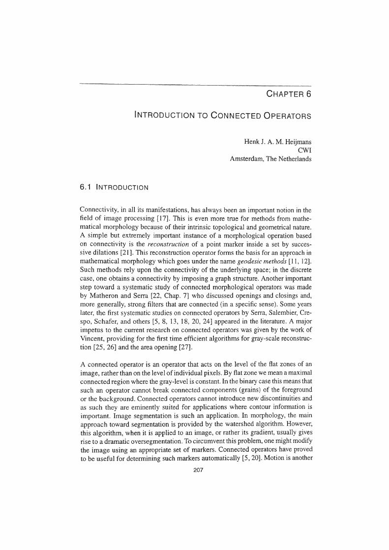
Here B is the 3 x 3 square. The algorithm is illustrated in Fig. 6-1.
The sets X and Y in p(Y IX) are called the mask (image) and marker (image),
respectively. Obviously, y1i(X) = p({h} IX), meaning that the opening Yh can be
computed with the aid of the algorithm given above.
210 CHAPTER 6
Figure 6-1. Reconstruction algorithm. From left to right: the mask image X (gray) and the marker image Y (black); 15 iterations; 50 iterations; final result p(Y IX).
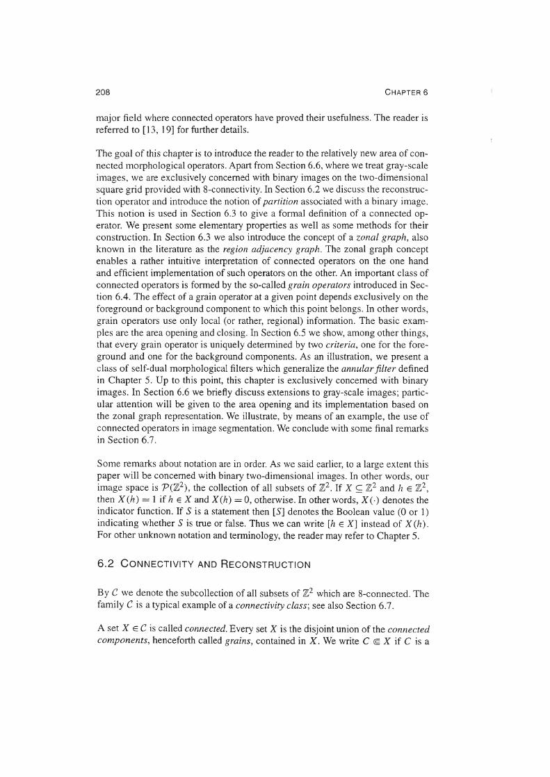
Figure 6-2. Dual reconstruction algorithm. From left to right: the mask image X (black) and the marker image Y (gray and black); 20 iterations; 75 iterations; final result p*(Y IX)
(gray and black).
The reconstruction operator yields a reconstruction of the foreground. Instead, we can also perform a reconstruction of the background. We call the resulting operator the background reconstruction or dual reconstruction, and denote it by p*:
Now the converse of Proposition 6-2 holds, namely
p*( nyi Ix) =np*(Yi IX), ie/ ie/
that is, the mapping Y 1-+ p*(Y IX) is an erosion. The dual reconstruction is illustrated in Fig. 6-2.
Observe that
p(Y IX)~ X ~ p*(Y IX),
for any two sets X, Y ~ 'l}.
By a partition of the space 'll} we mean a subdivision of this space into disjoint parts. A partition can be represented by a function P : Z2 ~ P('ll}) which has the following properties:
INTRODUCTION TO CONNECTED OPERATORS 211
_ _j
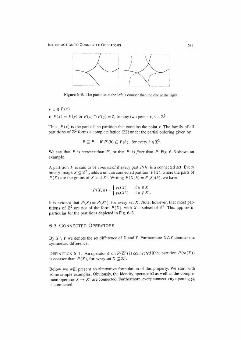
Figure 6-3. The partition at the left is coarser than the one at the right.
• x E P (x)
• P(x) = P(y) or P(x) n P(y) = 0, for any two points x, y E 'JI}.
Thus, P (x) is the part of the partition that contains the point x. The family of all
partitions of 'If} forms a complete lattice [22] under the partial ordering given by
P ~ P' if P'(h) s;; P(h), for every h E '1!}.
We say that P is coarser than P', or that P' is finer than P. Fig. 6-3 shows an
example.
A partition P is said to be connected if every part P (h) is a connected set. Every
binary image X s;; 'If} yields a unique connected partition P (X), where the parts of
P(X) are the grains of X and xc. Writing P(X, h) = P(X)(h), we have
if h EX if h ~ xc'.
It is evident that P (X) = P (X('), for every set X. Note, however, that most par
titions of Z2 are not of the form P (X), with X a subset of '11}. This applies in
particular for the partitions depicted in Fig. 6-3.
6.3 CONNECTED OPERATORS
By X \ Y we denote the set difference of X and Y. Furthermore X b.Y denotes the
symmetric difference.
DEFINITION 6-1. An operator if! on P('ll.2) is connected if the partition P ( 1f; (X))
is coarser than P (X), for every set X s;; 'If}.
Below we will present an alternative formulation of this property. We start with
some simple examples. Obviously, the identity operator id as well as the comple
ment operator X --+ xc are connected. Furthermore, every connectivity opening Yh
is connected.
212
, ..... , ' ' ' '
' ' ' ' '-'
CHAPTER 6
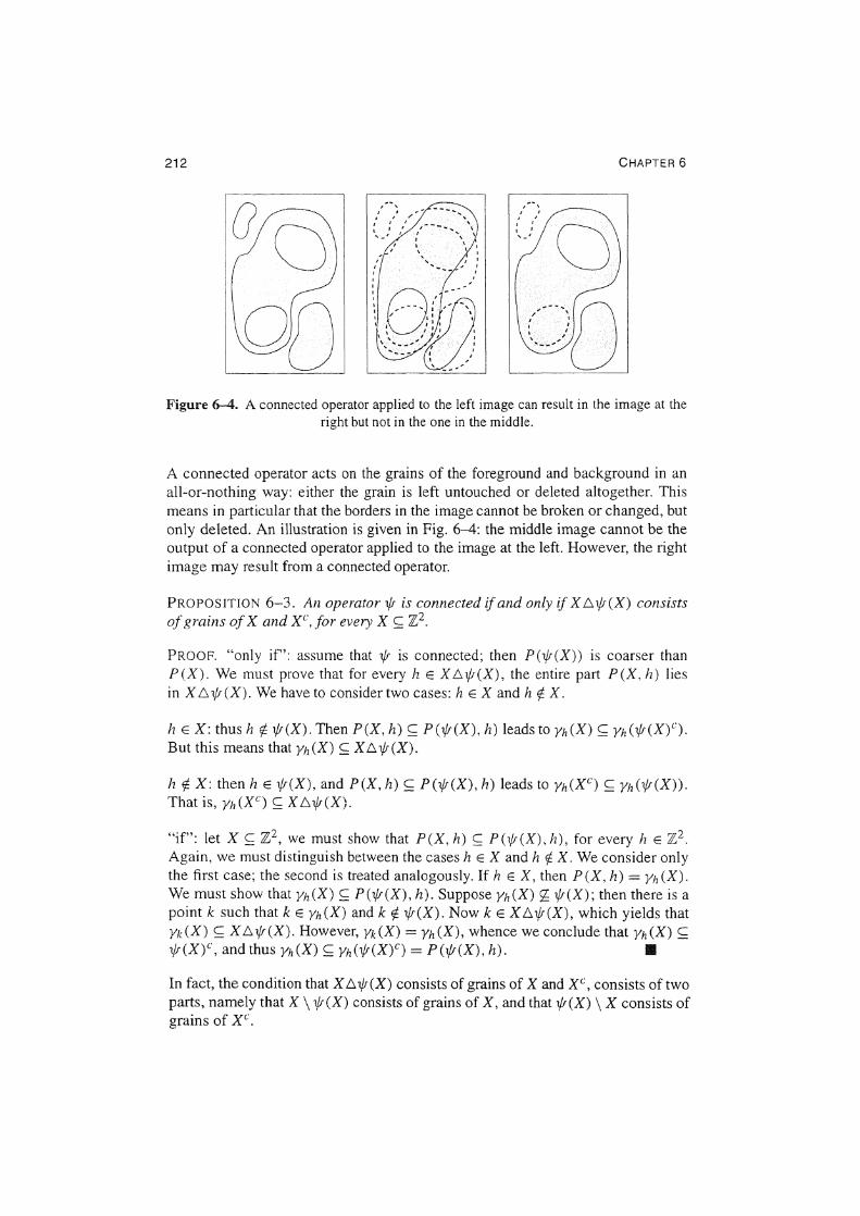
Figure 6-4. A connected operator applied to the left image can result in the image at the right but not in the one in the middle.
A connected operator acts on the grains of the foreground and background in an all-or-nothing way: either the grain is left untouched or deleted altogether. This means in particular that the borders in the image cannot be broken or changed, but only deleted. An illustration is given in Fig. 6-4: the middle image cannot be the output of a connected operator applied to the image at the left. However, the right image may result from a connected operator.
PROPOSITION 6-3. An operator 1/; is connected if and only if X 6.1/;(X) consists of grains of X and xc,Jor every X s; '71}.
PROOF. "only if": assume that 1/; is connected; then P(l/;(X)) is coarser than P(X). We must prove that for every h E X!:::..1/;(X), the entire part P(X, h) lies in X 6.1/; (X). We have to consider two cases: h E X and h fj. X.
h EX: thus h rj 1/;(X). Then P(X, h) s; P(l/;(X), h) leads to Yh(X) s; Yh(l/;(X)c). But this means that Yh(X) s; X!:::,,1/;(X).
h fj. X: then h E 1/;(X), and P(X, h) s; P(l/;(X), h) leads to Yh(Xc) s; Yh(l/l(X)). That is, Yh(Xc) s; X!:::,,1/;(X).
"if": let X s; 'll}, we must show that P(X, h) s; P(l/;(X), h), for every h E 'll}. Again, we must distinguish between the cases h E X and h f. X. We consider only the first case; the second is treated analogously. If h E X, then P (X, h) = Yh (X). We must show that Yh(X) s:; P(l/;(X), h).Suppose Yh(X) i 1/;(X); then there is a point k such that k E Yh (X) and k fj. 1/; (X). Now k E X 6.1/; (X), which yields that Yk(X) £:; X!:::..1/;(X). However, Yk(X) = Yh(X), whence we conclude that Yh(X) s:; 1/;(X)c, and thus Yh(X) £:; Yh(l/;(X)C) = P(l/;(X), h). •
In fact, the condition that X !:::,, 1/;(X) consists of grains of X and xc, consists of two parts, namely that X \ 1/;(X) consists of grains of X, and that 1/;(X) \ X consists of grains of xc.
INTRODUCTION TO CONNECTED OPERATORS 213
PROPOSITION 6-4. An operator 1/1 is connected ~f" and only if its negative 1/f* is connected.
PROOF. Assume that 1/1 is connected; then P(i/f(X)) !;: P(X), for every X s; '!}.
Substituting xc yields that
Using that P(i/f*(X)) = P(l/f(Xc)c) = P(i/f(X")), and that P(Xc:) = P(X), we
get that
P(i/f*(X)) !;: P(X).
This proves the result. • We present a number of results that show how to build new connected opera
tors from known ones using composition, supremum, infimum, as well as other
"Boolean combinations."
PROPOSITION 6-5. If o/1. o/2 are connected, then 1/f21/f1 is connected, too.
PROOF. This result is a simple consequence of Definition 6-1:
for every X s; 'l}, if 1/11 and 1/12 are connected. II
PROPOSITION 6-6. If 1/f; is a connected operator for every i in some index set I,
then the infimum j\iEI lfi and the Supremum viE/ 1/fi are connected, too.
PROOF. We first prove the result for the infimum. Let 1/f = /\iE/ 1/f;, then X \
1/f(X) = LJiE/(X \ 1/f;(X)) and 1/f(X) \ X = niE/(1/r;(X) \ X). As every set X \
1/li (X) is a union of grains of X, X \ 1/f (X) is also a union of grains of X. Similarly,
we have that 1/f (X) \ X is a union of grains of xc', and we conclude that 1/f is
connected.
The result for the supremum can be obtained analogously, but it also follows from
the observation that
in combination with Proposition 6-4. •
214 CHAPTER 6
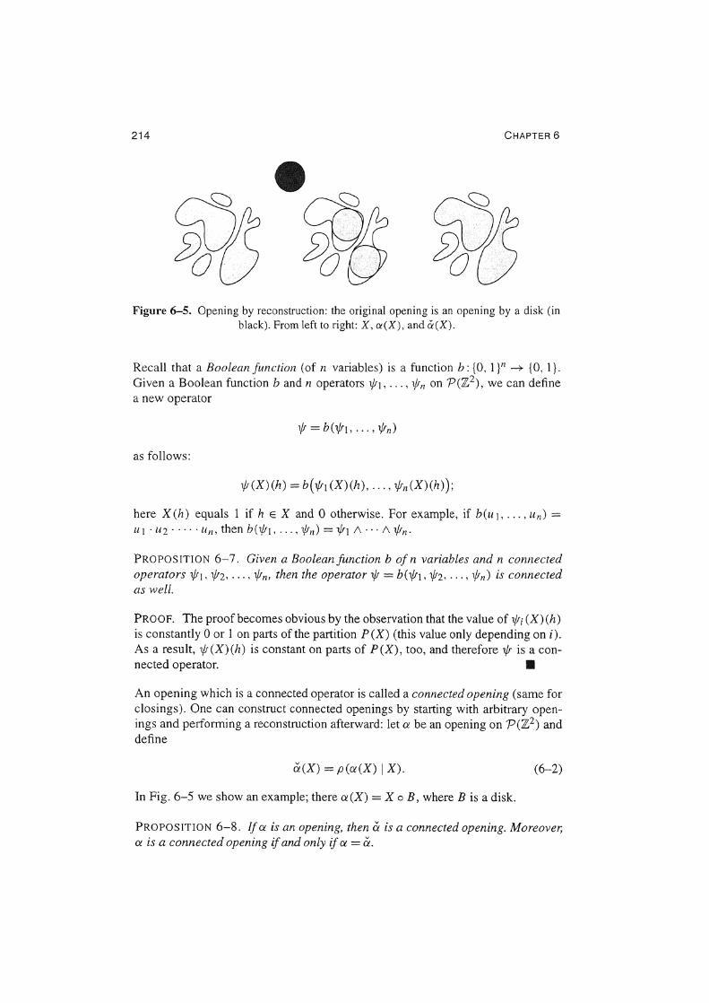
Figure 6-5. Opening by reconstruction: the original opening is an opening by a disk (in black). From left to right: X, a(X), and a(X).
Recall that a Boolean function (of n variables) is a function b: {O, 1 }n --+ {O, I}. Given a Boolean function band n operators 1/J1, ... , 1/Jn on P('J!}), we can define a new operator
as follows:
1/i(X)(h) = b(i/J1(X)(h), ... ,1/Jn(X)(h));
here X(h) equals 1 if h EX and 0 otherwise. For example, if b(u1, ... , un) = u J • 112 · · · · · lln, then b(1/J1, ... , 1/Jn) = 1/J1/\···/\1/Jn·
PROPOSITION 6-7. Given a Boolean function b of n variables and n connected operators 1/J1, 1/J2, ... , i/Jn. then the operator 1/J = b(1/J1, 1/J2, ... , 1/Jn) is connected as well.
PROOF. The proof becomes obvious by the observation that the value of 1/Ji (X) (h) is constantly 0 or 1 on parts of the partition P(X) (this value only depending on i). As a result, 1/J (X)(h) is constant on parts of P (X), too, and therefore 1/J is a con-nected operator. Ill
An opening which is a connected operator is called a connected opening (same for closings). One can construct connected openings by starting with arbitrary openings and performing a reconstruction afterward: let a be an opening on P(Z2) and define
a(X) =p(a(X) IX). (6-2)
In Fig. 6-5 we show an example; there a(X) = X o B, where Bis a disk.
PROPOSITION 6-8. If a is an opening, then a is a connected opening. Moreover, a is a connected opening if and only if a = a.
INTRODUCTION TO CONNECTED OPERATORS 215
•
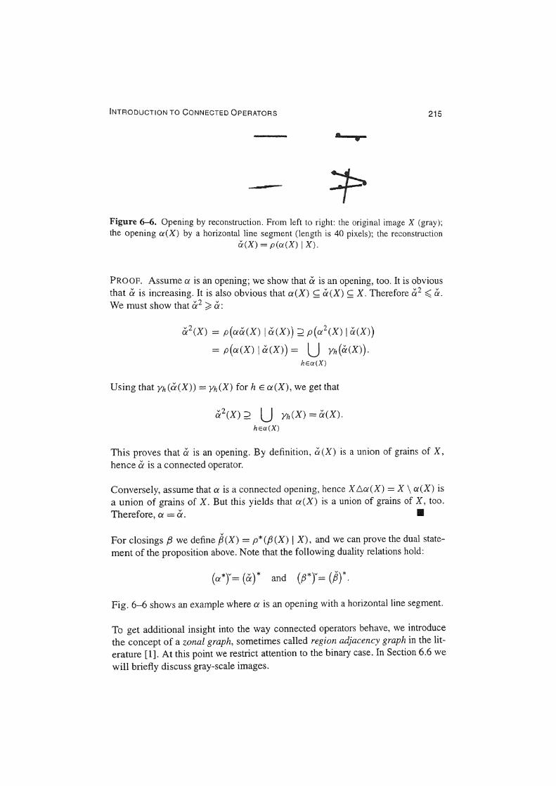
Figure 6-6. Opening by reconstruction. From left to right: the original image X (gray);
the opening a(X) by a horizontal line segment (length is 40 pixels); the reconstruction
a(X) = p(a(X) IX).
PROOF. Assume a is an opening; we show that a is an opening, too. It is obvious
that a is increasing. It is also obvious that a (X) s; a (X) s; X. Therefore Q- 2 ~ a. We must show that Q- 2 ;:::: a:
a2(X) = p(a&(X) I a(X)) 2 p(a2(X) I a(X))
= p(a(X) 1 a(X)) = LJ Yh(a(X)). hEa(X)
Using that Yh(a(X)) = Yh(X) for h E a(X), we get that
a2(X) 2 LJ Yh(X) =a(X). hEa(X)
This proves that a is an opening. By definition, a(X) is a union of grains of X,
hence a is a connected operator.
Conversely, assume that a is a connected opening, hence XL:o.a(X) = X \ a(X) is
a union of grains of X. But this yields that a(X) is a union of grains of X, too.
Therefore, a = & . II
For closings f3 we define ~ (X) = p* (/3 (X) I X), and we can prove the dual state
ment of the proposition above. Note that the following duality relations hold:
(a*r= (a)* and (/J*r= (~)*.
Fig. 6-6 shows an example where a is an opening with a horizontal line segment.
To get additional insight into the way connected operators behave, we introduce
the concept of a zonal graph, sometimes called region adjacency graph in the lit
erature [l]. At this point we restrict attention to the binary case. In Section 6.6 we
will briefly discuss gray-scale images.
216 CHAPTER 6
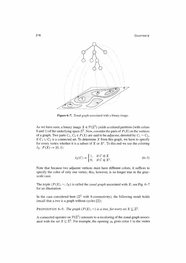
Figure 6-7. Zona! graph associated with a binary image.
As we have seen, a binary image X E P('l!}) yields a colored partition (with colors 0 and 1) of the underlying space 'll}. Now, consider the parts of P(X) as the vertices of a graph. Two parts C1, C2 E P (X) are said to be adjacent, denoted by C1 ,....., C2, if C1 U C2 is a connected set. To determine X from this graph, we have to specify for every vertex whether it is a subset of X or xc. To this end we use the coloring Ix: P(X)-+ {O, 1}:
Ix(C) = { l, 0,
if C CSX if C CS xc. (6-3)
Note that because two adjacent vertices must have different colors, it suffices to specify the color of only one vertex; this, however, is no longer true in the grayscale case.
The triple (P (X), "-', Ix) is called the zonal graph associated with X; see Fig. 6-7 for an illustration.
In the case considered here ('l} with 8-connectivity), the following result holds (recall that a tree is a graph without cycles [2]):
PROPOSITION 6-9. The graph (P (X),,.....,) is a tree,for every set X s;; '1!}.
A connected operator on P('ll2) amounts to a recoloring of the zonal graph associated with the set X s; 'll2 . For example, the opening Yh gives color 1 to the vertex
INTRODUCTION TO CONNECTED OPERATORS 217
~.···.·.··.·.·.·.·.· ... · ..•. ·.· •. · .. ••· •. ~ ..•• · •• · ••. · •... ·• .... ·.· .•. · •.. ·· •• ·•·.· •.• · •.•. · •..••. ··.d?.··.·· ... · •. · .• · ..• ·.·.···.·.·.········.······.·.·.···.·······~.·.>.)• ~ ........... · .... ······.····•.····.· .. ········•····.······· ~.· .. ·.·•·.··••·· ...•. · .. ·.··.··.•.·.· .. ·· .. · .. ·· ....... ·.· •. · .... ·.· .. ··.·.·.······~ di~ ~ y.~ •. ~,~··~ ~·/~ ;., .... _ ..... ,.:,-'.',''.', - - ::-,.•:•.; .. : ·:':!:<':-~-::-.:::::·,·:=::- '' - " •• ".
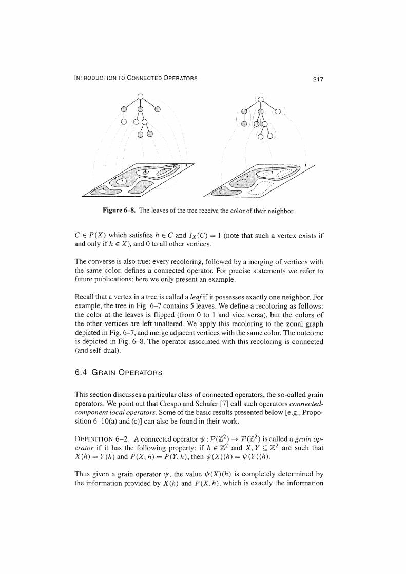
Figure 6-8. The leaves of the tree receive the col or of their neighbor.
C E P (X) which satisfies h E C and Ix ( C) = I (note that such a vertex exists if and only if h E X), and 0 to all other vertices.
The converse is also true: every recoloring, followed by a merging of vertices with the same color, defines a connected operator. For precise statements we refer to future publications; here we only present an example.
Recall that a vertex in a tree is called a leaf if it possesses exactly one neighbor. For example, the tree in Fig. 6-7 contains 5 leaves. We define a recoloring as follows: the color at the leaves is flipped (from 0 to 1 and vice versa), but the colors of the other vertices are left unaltered. We apply this recoloring to the zonal graph depicted in Fig. 6-7, and merge adjacent vertices with the same color. The outcome is depicted in Fig. 6-8. The operator associated with this recoloring is connected (and self-dual).
6.4 GRAIN OPERATORS
This section discusses a particular class of connected operators, the so-called grain operators. We point out that Crespo and Schafer [7] call such operators connectedcomponent local operators. Some of the basic results presented below [e.g., Proposition 6-lO(a) and (c)] can also be found in their work.
DEFINITION 6-2. A connected operator l.fr: PCll})--+ PC!!}) is called a grain operator if it has the following property: if h E '11} and X, Y s; Z2 are such that X(h) = Y(h) and P(X, h) = P(Y, h), then ij1(X)(h) = l./r(Y)(h).
Thus given a grain operator if;, the value o/(X)(h) is completely determined by the information provided by X (h) and P (X, h), which is exactly the information
218 CHAPTER 6
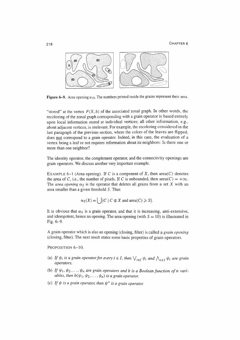
Figure 6-9. Area opening a 10 • The numbers printed inside the grains represent their area.
"stored" at the vertex P(X, h) of the associated zonal graph. In other words, the
recoloring of the zonal graph corresponding with a grain operator is based entirely
upon local information stored at individual vertices; all other information, e.g.,
about adjacent vertices, is irrelevant. For example, the recoloring considered in the last paragraph of the previous section, where the colors of the leaves are flipped, does not correspond to a grain operator. Indeed, in this case, the evaluation of a
vertex being a leaf or not requires information about its neighbors: Is there one or
more than one neighbor?
The identity operator, the complement operator, and the connectivity openings are
grain operators. We discuss another very important example.
EXAMPLE 6-1 (Area opening). If C is a component of X, then area(C) denotes the area of C, i.e., the number of pixels. If C is unbounded, then area(C) = +oo. The area opening as is the operator that deletes all grains from a set X with an area smaller than a given threshold S. Thus
as(X) = LJ{C [ C ~ X and area(C) ~ S}.
It is obvious that as is a grain operator, and that it is increasing, anti-extensive, and idempotent, hence an opening. The area opening (with S = 10) is illustrated in Fig. 6-9.
A grain operator which is also an opening (closing, filter) is called a grain opening (closing, filter). The next result states some basic properties of grain operators.
PROPOSITlON 6-10.
(a) If lfi is a grain Operator for every i E J, then ViE/ lfi and f\iEI lfi are grain operators.
(b) If 1/f 1, 1/f2, ... , lfn are grain operators and b is a Boolean function of n variables, then b(1/f1, 1/!2, ... , 1/!12 ) is a grain operator.
(c) If 1/f is a grain operator, then if!* is a grain operator.
INTRODUCTION TO CONNECTED OPERATORS 219
PROOF. (a) We show that 1/; = ViE/ ifi is a grain operator. The proof for the infimum is analogous. Leth, X, Y be such that X(h) = Y(h) and P(X, h) = P(Y. h);
we show that 1/;(X)(h) = 1/;(Y)(h). Obviously,
if(X)(h) = (v Vri(x))<h) = v ifi(X)(h). iEI iE/
Since every Vri is a grain operator, this last expression equals
v Vri (Y)(h) = ( v Vri(Y))(h) = 1/;(Y)(h), iE/ iEI
and this shows the result.
(b) Let 1/; = b(1/;1, if1 .... , ifn). By definition
1/;(X)(h) = b(1/;1 (X)(h), if1(X)(h), ... , 1/!n(X)(h) ),
and with this relation, the proof becomes similar to the proof of (a).
(c) This follows easily if one uses the relation 1/;*(X)(h) = 1 -1/;(Xc)(h). B
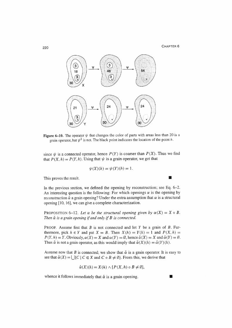
The composition of two grain operators, however, is not a grain operator, in general. In Fig. 6-10 we depict an example of a grain operator if for which 1/;2 is not a grain operator. The operator acts as follows: for every part of the partition P (X) it switches the color from I to 0, or vice versa, if the area of this part is below a given threshold (20 in this specific example). The value if2(X)(h) is different in the upper and lower figure, although X(h) = Y(h) = 1 and P(X, h) = P(Y, h). Therefore, if 2 is not a grain operator.
By the duality principle (see Chapter 5), every statement about openings has a dual version concerning closings. In what follows, we restrict ourselves to openings.
PROPOSITION 6-11. Every anti-extensive grain operator is idempotent. In particular, an increasing grain operator is an opening ~f and only if it is anti-extensive.
PROOF. Let 1/; be an anti-extensive grain operator. We must show that if is idempotent. The nontrivial part of the proof consists of showing that 1(1 2 ) 1/;. Assume that h E if(X); we must show that h E 1/;2 (X). Put Y = if(X), then X(h) = Y(h) = 1. This implies that
P(Y, h) = Yh(Y) ~ Yh(X) = P(X, h).
On the other hand,
P(X, h) ~ P(Y, h),
220 CHAPTER 6
Figure 6-10. The operator 1f! that changes the color of parts with areas less than 20 is a
grain operator, but ijJ2 is not. The black point indicates the location of the point h.
since if; is a connected operator, hence P (Y) is coarser than P (X). Thus we find
that P (X, h) = P (Y, h). Using that 1/J is a grain operator, we get that
1/f(X)(h) = 'ljJ(Y)(h) = 1.
This proves the result. II
In the previous section, we defined the opening by reconstruction; see Eq. 6-2. An interesting question is the following: For which openings et is the opening by
reconstruction a a grain opening? Under the extra assumption that et is a structural
opening [10, 16], we can give a complete characterization.
PROPOSITION 6-12. Let a be the structural opening given by et(X) = X o B.
Then a is a grain opening if and only if B is connected.
PROOF. Assume first that B is not connected and let Y be a grain of B. Fur
thermore, pick h E Y and put X =B. Then X(h) = Y(h) = 1 and P(X, h) = P(Y, h) = Y. Obviously, a(X) = X anda(f) = 0, hence a(X) = X and a(f) = 0.
Thus a is not a grain operator, as this would imply that a(X)(h) = a(Y)(h).
Assume now that B is connected; we show that a is a grain operator. It is easy to
see that a(X) = LJ{C I c <S x and c 0 B =j=. 0}. From this, we derive that
ct(X)(h) = X (h) /\ [P (X, h) o B =j=. 0],
whence it follows immediately that a is a grain opening. II
INTRODUCTION TO CONNECTED OPERATORS 221
PROPOSITION 6-13. An opening a is a grain opening if and only if a=
vhEZ2 ayh.
PROOF. Assume that a is a grain opening. It is trivial that a ? VxEz2 ayx; therefore, we only have to show that a :::;; V x EZ2 ayx. Suppose that h E a (X). Define Y = Y11(X), then X(h) = Yh(X)(h) = I. Furthermore, P(X, h) = Yh(X) = P(Y, h).Since a is a grain operator, we get that a(X)(h) = a(Y)(h), and this implies that h E a(Y) = ctyh(X) ~ V xEZ2 ctyx(X).
To prove the converse, assume that a = V xEz2 ayx; we show that a is a grain operator. Suppose that X(h) = Y(h) and P(X, h) = P(Y, h).We must show that a(X)(h) = a(Y) (h). If X (h) = 0, this is trivial; we consider the case that X (h) = 1. Thus P(X, h) = Yh(X) = Yh(Y). Now
a(X)(h) = ( V ayt(X)) (h) = V ayx(X)(h)
xEZ2 xEZ2
This concludes the proof.
= ctyh(X)(h) = ayh (Y)(h)
= a(Y)(h).
II
Recall that a set B is invariant under an operator 1f.r if 'lj.r(B) =B. We will show that any subset of grains of a set X invariant under a grain filter 1f.r is also invariant under 1f.r. Refer to (22, Chap. 7) for some related results. We start with a lemma.
LEMMA 6-1. let 1/r he an increasing connected operator on P('l}), and let X ~ '1!} satisfy 'lj.r(X) ~ X. If Y is a union of grains of X, then 'lj.r(Y) ~ Y.
PROOF. Suppose that 1f.r (Y) g; Y. Since 1f.r is connected, 1f.r (Y) \ Y consists of grains of ye_ Let D be a grain of ye contained in 'lj.r(Y) \ Y. We show that D n xc # 0. Suppose that D ~ X. The grain D must be adjacent to a grain C of Y, meaning that C U D is connected. However, C U D ~ X, and we conclude that C cannot be a grain of X. But this contradicts our assumption that Y consists of grains of X. Thus D n X'-' # 0.
Since D ~ 'lj.r(Y) and 1f.r is increasing, also D ~ 'lj.r(X). This yields that 'lj.r(X) n xc # 0, i.e., X n xc # 0, a contradiction. We conclude that 'lj.r(Y) ~ Y, as asserted.
PROPOSITION 6-14. let 1f.r be a grain filter and 'lj.r(X) = x.
(a) If Y is a union of grains of X, then 1f.r (Y) = Y.
(b) If Y is a union of grains of xc, then 'lj.r(fl') =ye_
II
222 CHAPTER 6
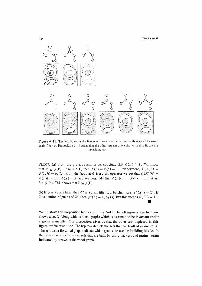
Figure 6-11. The left figure in the first row shows a set invariant with respect to some
grain filter if;. Proposition 6-14 states that the other sets (in gray) shown in this figure are invariant, too.
PROOF. (a) From the previous lemma we conclude that 1/f (Y) ~ Y. We show
that Y ~ 1/f(Y). Take h E Y, then X(h) = Y(h) = 1. Furthermore, P(X, h) = P ( Y, h) = Yh ( X). From the fact that if; is a grain operator we get that if; ( X) ( h) = ij;(Y)(h). But i.j;(X) = X and we conclude that 1/;(Y)(h) = X(h) = 1, that is,
h E 1/f(Y). This shows that Y s; i.j;(Y).
(b) If i/! is a grain filter, then i.J;* is a grain filter too. Furthermore, if;* (Xc) = xc. If Y is a union of grains of xc, then 1/;*(Y) = Y, by (a). But this means 1/;(fL') =ye_
11111
We illustrate this proposition by means of Fig. 6-11. The left figure at the first row
shows a set X (along with its zonal graph) which is assumed to be invariant under
a given grain filter. Our proposition gives us that the other sets depicted in this
figure are invariant, too. The top row depicts the sets that are built of grains of X.
The arrows in the zonal graph indicate which grains are used as building blocks. In
the bottom row we consider sets that are built by using background grains, again indicated by arrows in the zonal graph.
INTRODUCTION TO CONNECTED OPERATORS 223
6.5 GRAIN OPERATORS AND GRAIN CRITERIA
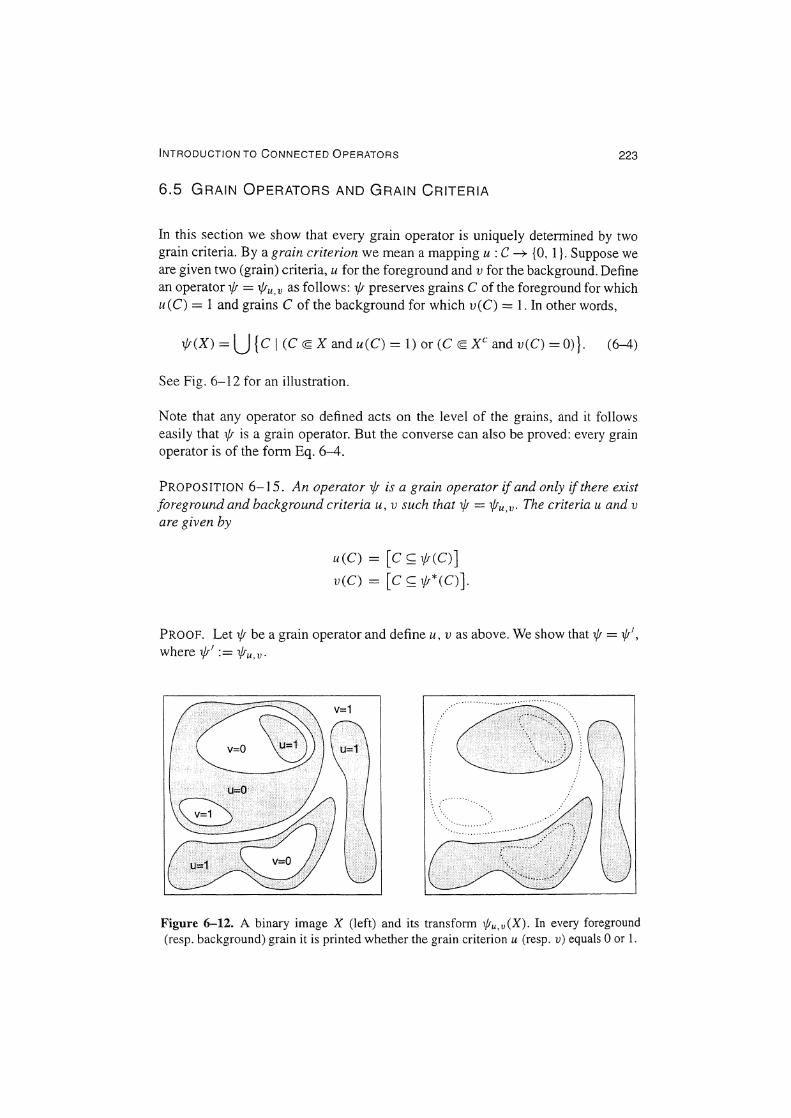
In this section we show that every grain operator is uniquely determined by two grain criteria. By a grain criterion we mean a mapping u : C--+ {O, 1 }. Suppose we are given two (grain) criteria, u for the foreground and v for the background. Define an operator 1/1 = 1/Ju, v as follows: 1/1 preserves grains C of the foreground for which u(C) = 1 and grains C of the background for which v(C) = 1. In other words,
1/f(X) = LJ { C I (C <S X and u(C) = 1) or (C <S xc and v(C) = 0) }. (6-4)
See Fig. 6-12 for an illustration.
Note that any operator so defined acts on the level of the grains, and it follows easily that 1/1 is a grain operator. But the converse can also be proved: every grain operator is of the form Eq. 6-4.
PROPOSITION 6-15. An operator 1/1 is a grain operator if and only if there exist foreground and background criteria u, v such that 1/1=1/Ju,v· The criteria u and v are given by
u ( C) = [ C £;; 1/1 ( C) J v(C) = [c £;; 1/f*(C)].
PROOF. Let 1/1 be a grain operator and define u, v as above. We show that 1/1 = 1/J', where 1/1' := 1/lu,v·
Figure 6-12. A binary image X (left) and its transform i/Ju,v(X). In every foreground (resp. background) grain it is printed whether the grain criterion u (resp. v) equals 0 or 1.
224 CHAPTER 6
First we show that if!(X) s; y/ (X) for every set X. Let C be a part of P (X) and
Cs; 1/r(X); we show that Cs; if!'(X). We distinguish two cases.
( l ). C cs X. We show that u ( C) = 1, for then C s; 1/r' (X). We must prove that C s;;:
1/r(C). Leth EC, then C(h) = X(h) = I and P(X, h) = P(C, h) =C. Since 1/1 is a grain operator, we may conclude that ij;(X)(h) = ij;(C)(h). Since Cs;;: ij;(X),
this expression equals 1, and we conclude that h E if; ( C). Therefore, C s;;: if; ( C).
(2). C cs xc. We show that Cs; ij;(C'"), which yields that v(C) = 0. Leth EC,
then cc(h) = X(h) = 0. Furthermore, P(Cc, h) = P(X, h) = C, and using that
if; is a grain operator, we get that ij;(X)(h) = ij;(Cc)(h). Since Cs; ij;(X), this
expression equals 1, and we conclude that h E ij;(C"). Therefore, Cs;;: 1/f(Cc).
Next we show that if!'(X) s; if!(X). Assume that C is a part of P(X) and that
C s; 1/f' (X). We show that C s; if! (X). Again, we distinguish two cases.
(1). C cs X. Then u(C) = 1, hence Cs; if!(C). Leth EC, then C(h) = X(h) =I
and P ( X, h) = P ( C, h) = C, and, by the fact that if; is a grain operator, we get that
ij;(X)(h) = ij;(C)(h) = 1. This shows that Cs; ij;(X).
(2). C cs xc. Then v(C) = 0, which yields that C s;; ij;(Cc). Let h EC, then
c·(h) = X(h) = 0 and P(X,h) = P(C'",h) = C, and we get that ij;(X)(h) =
if!(Cc)(h). Since Cs; ij;(Cc), this expression equals 1, and we conclude that
Cs; 1/f(X).
This concludes our proof.
A criterion u is called increasing if C, C' EC and Cs; C' implies that u(C) :(
u(C'). One might expect that if;= i/lu,v is increasing when both criteria u and v
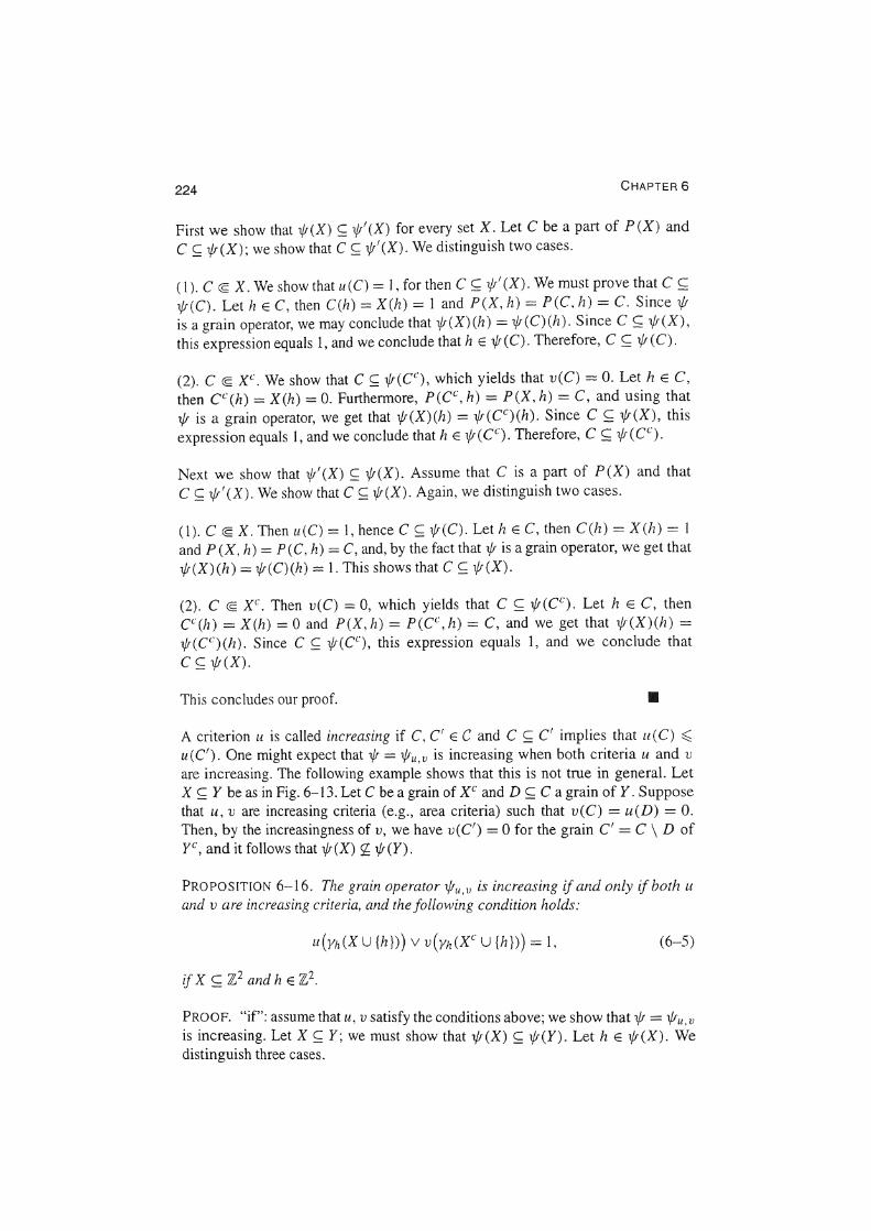
are increasing. The following example shows that this is not true in general. Let
X s; Y be as in Fig. 6-13. Let C be a grain of xc and D s; C a grain of Y. Suppose
that u, v are increasing criteria (e.g., area criteria) such that v(C) = u(D) = 0. Then, by the increasingness of v, we have v(C') = 0 for the grain C' = C \ D of ye, and it follows that i/t(X) g; 1/J(Y).
PROPOSITION 6-16. The grain operator i/lu,v is increasing if and only if both u and v are increasing criteria, and the following condition holds:
(6-5)
if X s; 'l/} and h E 'f}.
PROOF. "if": assume that u, v satisfy the conditions above; we show that 1/f = 1/fu,v
is increasing. Let X s; Y; we must show that ij;(X) s; ij;(Y). Leth E ij;(X). We distinguish three cases.
INTRODUCTION TO CONNECTED OPERATORS 225
y
Figure 6-13. if; is not increasing. Indeed, X s=;: Y but i/!(X) Sf ij;(Y).
1. h EX: put C = Y1i(X), then C CSX and Cc; C' = Yh(Y). Ash E 1/!(X), we have
u(C) =I, and since u is increasing u(C') = 1, giving that h E 1/!(Y).
2. h tf. Y: put C' = Yh (Ye) and C = Yh (Xc), then C' c; C since ye c; xc. From the
fact that h E 1/!(X) we conclude that u(C) = 0 and thus u(C') = 0, yielding that
h E if(Y).
3. h E Y and h rf:. X: suppose h rf:.1/!(Y), then u(yh(Y)) = 0. Now Eq. 6-5 implies
that u(Y11 (fl' U {h})) = l. Obviously, y1i(Y1' U {h}) c; y1i(X1'), and since vis in
creasing, we get that v(y,1 (X'')) = I. However, this implies that the grain Yh (Xc)
does not lie in if(X), contradicting h E if(X). Thus we conclude that h E if(Y).
"only if": assume that 1/1=1/111 .v is increasing. First we show that u is an increas
ing grain criterion. The proof that v is increasing is analogous. Let C s; C' be
connected, then if ( C) c; 1/1 ( C'). Suppose that u ( C) = 1, then C c; if ( C), hence
Cc; if(C'). Thus we get that Cc; C' n if(C'), and we conclude that u(C') = l
since otherwise C' n 1/!(C') = 0. Thus it remains to show Eq. 6-5. Let X c; Z 2
and u (y1i (X U {h})) = 0; we must show that v(yh (X" U {h})) = 1. Indeed, since
h rf:. if(X U {h}) and if is increasing, it follows that h rf:. t/,r(X \ {h}). This means
that v(P(X \ {h}, h)) = l. Now
P(X \ {h}, h) = Y1i((X \ {h})c) = Yh(Xc U {h}).
This yields the result. II
We write u = 1 if the criterion u is identically 1, i.e., u ( C) = 1 for every grain C.
When v = I, we write t/,r u, 1 for Vru, v. Similarly, o/1, v denotes the grain operator for
which the foreground criterion u is identically 1 .
EXAMPLE 6-2. We present some examples of grain criteria.
226 CHAPTER 6
• u(C) = C(h). Now ifru,I equals the connectivity opening Yh·
• u(C) = [area(C)): S]. The operator 1/.ru,1 is the area opening considered in Ex
ample 6-1.
• u ( C) = [perimeter( C) ): SJ, where perimeter( C) equals the number of bound
ary pixels in C. This criterion is not increasing.
• u ( C) = [area( C) /(perimeter( C) )2 ): k]. Note that this criterion provides a mea
sure for the circularity of C. This criterion is not increasing.
• 11 ( C) = [ C e B f 0], which gives the outcome 1 if some translate of B fits inside
C. If B is connected, then 1/ru, 1 =a, where a (X) = X o B; cf. Proposition 6-12.
However, if B is not connected, then ifru. 1 is an opening that is smaller than a, i.e., 1/ru,l ~a.
Breen and Jones [4] discuss various other increasing and nonincreasing criteria.
We state some other useful properties.
PROPOSITION 6-17.
(a) ifr1:.v = ifrv,u·
(b) Given grain operators i/lu;,v;.for i E /,then
/\ lf.ru;,v; = i/f /\iEI u;,ViEI v; iE/
and V i/lu;,v; = ifrviEI u;,f\;EJ v;.
iE/
(c) Let i/lu;,v; be grain operators for i = 1, 2, ... , n, and let b be a Booleanjimc
tion of n variables, then
Here b* denotes the negative of b given by b*(iq, ... , Un) = 1 - b(l -
U\, ... , l - Un).
PROOF. We prove only (c). In Proposition 6-lO(b) we have seen that ijf =
b( 1f.r u 1 , v1 , ••. , 1f.run, vn) is a grain operator. Therefore, 1fr is of the form 1f.r u, v. From
Proposition 6-15 we know that the foreground criterion u is given by u ( C) =
[ C s; 1fr ( C)]. Since if; is a grain operator, [ C f 1f1 ( C)] = [h E 1fr ( C)], for every h E
C. But this last expression equals b(1f.ru 1,v1 (C)(h), ... , ifrun,vn (C)(h)). Using that
i/lu;,v; (C)(h) = [C f i/lu;,v; (C)] = u;(C), we finally arrive at the identity u(C) = b(u 1 (C), ... , Un (C)). In a similar way we find that v(C) = b*(v1 (C), ... , Vn (C)),
and the result is proved. 1111
The following result is obvious:
INTRODUCTION TO CONNECTED OPERATORS 227
PROPOSITION 6-18. The grain operator 1/!u,v is extensive if and only ifu = 1. lt is anti-extensive if and only if v = 1.
We have seen that a composition of grain operators is not a grain operator, in general. However, it is easy to see that a composition of (anti-) extensive grain operators is an (anti-) extensive grain operator. To be precise
1/1 u2, 11/! u 1, I = 1/1u1, 11/! u2. I = 1/1u1 /\u2. I = 1/1u1, I /\ 1/1112 ,I ( 6-6)
1/!1,v21/!i,v1=1/!1,v11/!l,v2=1/!1,v1/\v2 = Vrl,v1 V Vrl.v2· (6-7)
Rather than presenting a formal proof of these relations (in fact, such a proof is rather straightforward, and we leave it as an exercise for the reader), we sketch only the underlying idea. The composition 1fru2,11fr111 ,1 cannot add background grains, but only delete foreground grains. A foreground grain C will be deleted in either of the two following situations: (i) u1 (C) = O; (ii) u1(C)=1 but u2(C) = 0. In other words, C is deleted if at least one of the criteria u 1 or u2 is not satisfied. Therefore, the foreground grain criterion for the composition 1fr u2 .11/r u 1, I is u = u 1 /\ u 2.
Taking u1 = u2 = u in Eq. 6-6, we find that lfr'!; 1 = Vru,I· Note in particular that this provides an alternative proof for Proposition '6-11.
As a special case of Eq. 6-6 we mention the identity
for every grain opening a. Taking the supremum over h E 'l} and using that V hez2 Yh =id, we arrive at the identity in Proposition 6-13.
In a forthcoming paper we will examine the construction of morphological filters that are connected. Here we discuss one specific example, namely the generalization of the (self-dual) annular filter on P('ll}) (see Chap. 5). We start with a lemma.
LEMMA 6-2. Given X s; Z2 and h E Z2, put C = P(X, h).If area(C):::;; 7 then C is a leaf of the zonal graph (tree) of X and the unique neighbor C' of C satisfies area( C') ~ 8. Moreover, C' U {h} is connected.
Verification of the validity of this lemma is just a matter of checking all possibilities, and is left as an exercise for the reader. The estimate area ( C') ~ 8 is sharp only if C comprises one pixel. It is easy to verify that we can replace the value 8 by 10, 12, 12, 14, 14, 16 for area(C) = 2, 3, 4, 5, 6, 7, respectively. But for our purposes, the estimate in the lemma is good enough.
Consider the increasing area criterion
us(C) = [area(C) ~ S],
228 CHAPTER 6
and define
It is evident that ws is a self-dual grain operator. Note that w1 =id.
PROPOSITION 6-19. If S:::; 8, then ws is a self-dual grain.filter.
PROOF. We must show that ws is increasing and idempotent. To show that ws
is increasing, we apply Proposition 6-16. It is evident that us is increasing. We
must show that condition 6-5 holds for u = v = us. Take X £ 'l}. Without
loss of generality we may assume that h E X. Put C = Yh (X), and suppose that
us(C) = 0. Now, the previous lemma yields that C is a leaf of the zonal tree of X,
which has a unique neighbor C' <S xc. Furthermore, C' U {h} is connected, thus
Yh (Xc U {h}) = C' U {h}, and the lemma says that the area of this component is
greater than or equal to 9. Thus us(Yh (Xc U {h})) = 1, which had to be shown. We
conclude that ws is increasing.
Now we show that ws is idempotent. Since cvs is self-dual, it is sufficient to show
that ws:::; w~. Let C be a part of P(X) and C £ ws(X). We must show that C £ w~(X). We distinguish two cases.
1. C <S X: since C is preserved by ws, it follows that us(C) = I. Since us is
increasing, the grain C' of ws(X) that contains C automatically obeys us(C') = 1,
and therefore C £ C' £ w~ (X).
2. C <S xc: in view of the fact that C £ ws(X), we have us(C) = 0. Thus
area( C) < S, in particular, area( C) :::; 7. Now the previous lemma yields that
C is a leaf of the zonal graph of X, and that its (unique) neighbor C' satisfies
area(C') ): 8, hence us(C') = 1. This means that the connected set CUC' lies
in cvs(X). Let C" be the grain of ws(X) containing CUC', then us(C") = I.
Therefore C" £ w~(X), in particular C £ w~(X). Ill
The filter w2 is the annular filter discussed in Chapter 5. Note that ws, for S:::; 8, is
the composition of the area opening as= i/fus, 1 and the area closing f3s = o/1, 115 ,
that is,
ws = asf3s = f3sas.
The compositions asf3s and f3sas are filters for every S ); 1. In general, these
two compositions are different. However, by our previous result, they coincide and
define a self-dual grain operator if S :o:;: 8. An illustration is given in Fig. 6-14.
INTRODUCTION TO CONNECTED OPERATORS 229
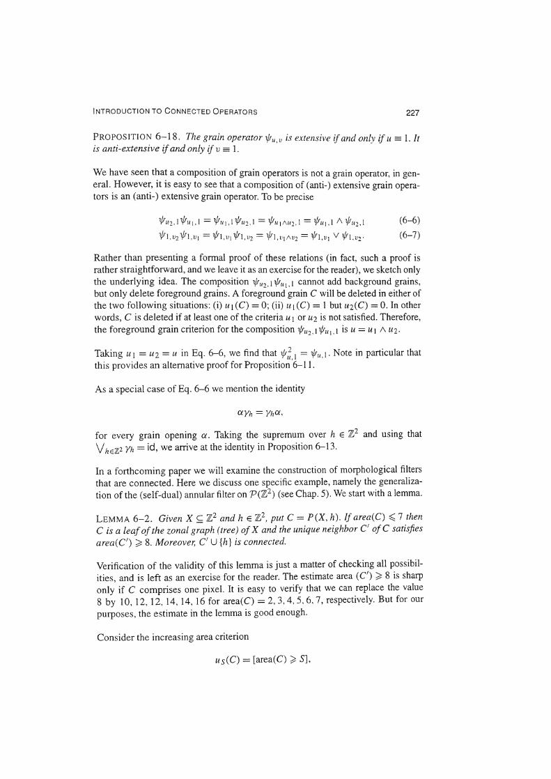
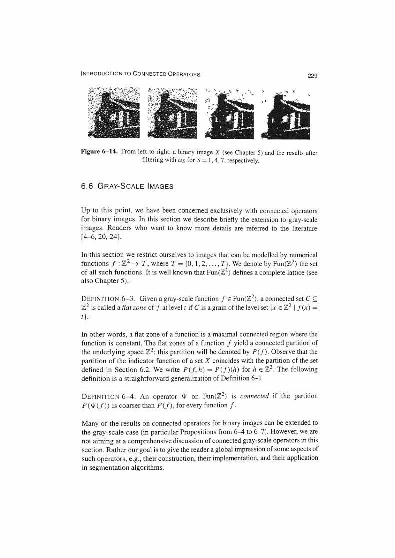
Figure 6-14. From left to right: a binary image X (see Chapter 5) and the results after filtering with ws for S = 1, 4, 7, respectively.
6.6 GRAY-SCALE IMAGES
Up to this point, we have been concerned exclusively with connected operators for binary images. In this section we describe briefly the extension to gray-scale images. Readers who want to know more details are referred to the literature [4-6, 20, 24].
In this section we restrict ourselves to images that can be modelled by numerical functions f: Z2 --+ T, where T = {O, 1, 2, ... , T}. We denote by Fun(Z2) the set of all such functions. It is well known that Fun(Z2) defines a complete lattice (see also Chapter 5).
DEFINITION 6-3. Given a gray-scale function f E Fun(Z2), a connected set C s; Z2 is called a.fiat zone off at level t if C is a grain of the level set {x E Z2 If (x) = t}.
In other words, a flat zone of a function is a maximal connected region where the function is constant. The flat zones of a function f yield a connected partition of the underlying space Z2 ; this partition will be denoted by P (J). Observe that the partition of the indicator function of a set X coincides with the partition of the set defined in Section 6.2. We write P(f, h) = P(f)(h) for h E 2 2. The following definition is a straightforward generalization of Definition 6-1.
DEFINITION 6-4. An operator '11 on Fun(Z2) is connected if the partition P ( '11 (f)) is coarser than P (f), for every function f.
Many of the results on connected operators for binary images can be extended to
the gray-scale case (in particular Propositions from 6-4 to 6-7). However, we are not aiming at a comprehensive discussion of connected gray-scale operators in this section. Rather our goal is to give the reader a global impression of some aspects of such operators, e.g., their construction, their implementation, and their application in segmentation algorithms.
230 CHAPTER 6
An important class of gray-scale operators is formed by the so-called flat opera
tors [9, 10]. Given an increasing operator ifr on P(l!}), there exists a unique increasing operator '*1 on Fun(Z,2) such that the following relation holds:
X('l'(f), t) = ifr(X(j, t)),
for f E Fun(Z2) and t ET. Here X(f, t) = {x E Z2 i f(x)? t} is the threshold set associated with f. We say that '*1 is generated by ifr. The following result can be established (a formal proof will be given in a future publication).
PROPOSITION 6-20. Let ifr be an increasing connected operator on P('l}). Then
the flat operator '*1 on Fun(:Z2) generated by ifr is connected, too.
In Section 6.3 we introduced the zonal graph for binary images. In fact, the same definition carries over to the gray-scale case. In this case, however, the coloring defined in Eq. 6-3 becomes a function If : P (f) --+ T. The zonal graph representation of a gray-scale function is tailor-made for the implementation of connected operators. This is best illustrated by means of an example. We consider the (flat extension of the) area opening with threshold S, and present an algorithm for its computation based upon the zonal graph representation of a gray-scale function f. Starting at the maximum gray-level (or color) t = T, we determine for each flat zone at level t if its area is greater than or equal to S. If so, then the output image receives the col or t for every pixel in this zone, insofar as it hasn't been set at a previous step. If not, that is, if the area is less than S, then the color t is diminished by one. After this last step, a flat zone may have one or more neighbors with the same color. Such zones are then merged into one new flat zone. This procedure has to be repeated until the minimum color is attained. Thus we arrive at the following algorithm.
• initialization input image I; output image l'(x) .f-0, all x;
•find all flat zones corresponding with /; /* now I is defined at flat zones */
• t *-T; /* T is maximum gray value */
•while t=f.O do { for every flat zone C with /(C)=t do
if area( C) ? S then for every x EC: J'(x) *- max{l'(x), t};
/(C) +-- t - I;
merge C with neighbors C' with I (C') = t - l;
f* areas of flat zones that are merged can be added */
t+-t-1;
INTRODUCTION TO CONNECTED OPERATORS 231
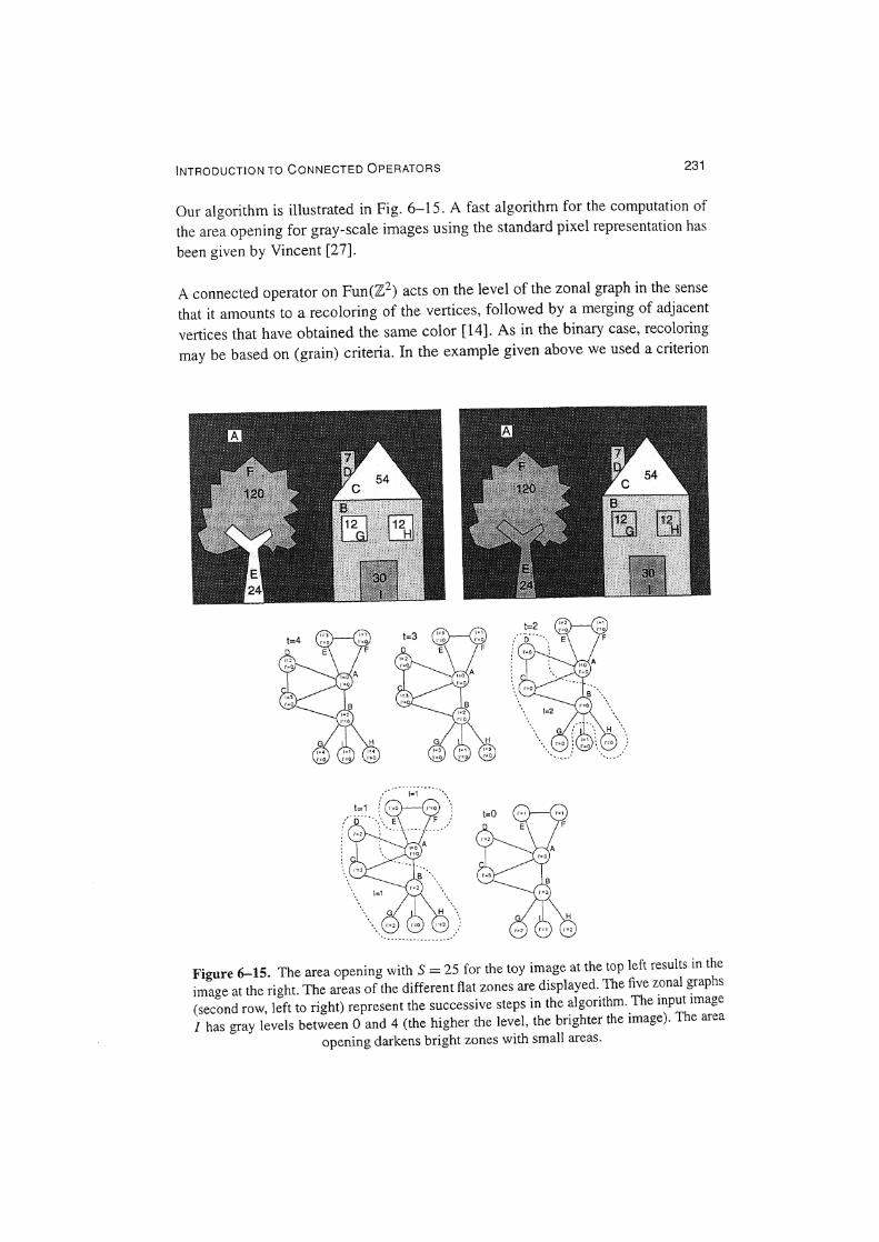
Our algorithm is illustrated in Fig. 6-15. A fast algorithm for the computation of
the area opening for gray-scale images using the standard pixel representation has
been given by Vincent [27]_
A connected operator on Fun(Z2) acts on the level of the zonal graph in the sense
that it amounts to a recoloring of the vertices, followed by a merging of adjacent
vertices that have obtained the same color [14]_ As in the binary case, recoloring
may be based on (grain) criteria_ In the example given above we used a criterion
Figure 6-15. The area opening with S = 25 for the toy image at the top left results in the
image at the right. The areas of the different flat zones are displayed. The five zonal graphs
(second row, left to right) represent the successive steps in the algorithm. The input image
I has gray levels between 0 and 4 (the higher the level, the brighter the image). The area
opening darkens bright zones with small areas.
232 CHAPTER 6
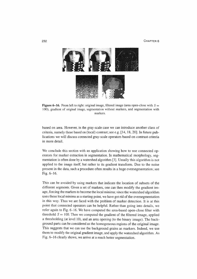
Figure 6-16. From left to right: original image, filtered image (area open-close with S = 100), gradient of original image, segmentation without markers, and segmentation with
markers.
based on area. However, in the gray-scale case we can introduce another class of criteria, namely those based on (local) contrast; see e.g. [14, 18, 20]. In future publications we will discuss connected gray-scale operators based on contrast criteria in more detail.
We conclude this section with an application showing how to use connected operators for marker extraction in segmentation. In mathematical morphology, segmentation is often done by a watershed algorithm [3]. Usually this algorithm is not applied to the image itself, but rather to its gradient transform. Due to the noise present in the data, such a procedure often results in a huge oversegmentation; see Fig. 6-16.
This can be avoided by using markers that indicate the location of subsets of the different segments. Given a set of markers, one can then modify the gradient image, forcing the markers to become the local minima; since the watershed algorithm uses these local minima as a starting point, we have got rid of the oversegmentation in this way. Thus we are faced with the problem of marker detection. It is at this point that connected operators can be helpful. Rather than going into details, we refer again to Fig. 6-16. We have computed the area-based open-close filter with threshold S = 100. Then we computed the gradient of the filtered image, applied a thresholding (at level l 0), and an area opening (to the binary image). The background parts can be considered as the homogeneous regions of the original image. This suggests that we can use the background grains as markers. Indeed, we use them to modify the original gradient image, and apply the watershed algorithm. As Fig. 6-16 clearly shows, we arrive at a much better segmentation.
INTRODUCTION TO CONNECTED OPERATORS 233
6. 7 CONCLUDING REMARKS
As the title of this chapter suggests, it contains an introduction to the theory of connected morphological operators. Our exposition is restricted to the case of binary images on a two-dimensional discrete 8-connected grid, with the exception of the previous section, which contains some results for the gray-scale case. We point out, however, that many of our results carry over to other image spaces and/or other notions of connectivity.
Serra [22] has introduced the notion of connectivity class for the complete Boolean lattice P(E), where Eis an arbitrary set; see also [10, 15].
DEFINITION 6-5. A family Cs; P(E) is a connectivity class if
• 0 E C and { h} E C, for every h E E;
• if xi EC, i E /,and niE/ xi =fa 0, then uiE/ xi E c.
This definition includes the class of 8-connected sets in Z2 (as well as the 4-connected sets), but one can find many other examples; see [15] for some interesting ones. Recently, Serra [23] has given an extension of the definition of connectivity class to other complete lattices than P(E).
Given a connectivity class C, we can define the connectivity openings Yh : P(E) -+ P(E) as follows:
Yh(X) = LJ{c EC\ h EC and Cs; X}.
To show that Yh is indeed an opening, we observe first that Yh is increasing and anti-extensive, hence that y~ ~ Yh. On the other hand, Yh (X) is a union of sets C E C with h E C s; X. Every C with this property satisfies C s; Yh (X), and this yields that Yh (X) s; Yf(X). Now we can define the reconstruction operator pas in Eq. 6-1. As a matter of fact, many of the definitions and results stated in this paper carry over to this general framework. We will not elaborate on this theme here.
Another issue that we have not explored in this chapter is the theory of connected filters other than openings and closings. Readers interested in this topic are referred to [8, 13, 20, 22].
ACKNOWLEDGMENT
The author gratefully acknowledges interesting discussions with Jose Crespo, Fernand Meyer, Philippe Salembier, and Jean Serra about various aspects of connected operators at the seminar on connected operators, June 14-15, 1996, in Barcelona.
234 CHAPTER 6
REFERENCES
[1] Ballard, D. H., and M. Brown, Computer Vision, Prentice-Hall, Englewood
Cliffs, NJ, 1982. [2] Berge, C., Graphs, 2nd ed., North-Holland, Amsterdam, 1985. (3] Beucher, S., and F. Meyer, "The morphological approach to segmentation:
the watershed transformation," in Mathematical Morphology in Image Processing, E. R. Dougherty, ed., Ch. 12, pp. 433-481, Marcel Deker, New York,
1993. (4] Breen, E., and R. Jones, "An attribute-based approach to mathematical mor
phology," in Mathematical Morphology and its Applications to Image and
Signal Processing, P. Maragos, R. W. Schafer and M.A. Butt, eds., pp. 41-
48, Kluwer Academic Publishers, Boston, 1996. [5] Crespo, J., Morphological connected filters and intra-region smoothing for
image segmentation, PhD thesis, Georgia Institute of Technology, Atlanta,
1993. [6] Crespo, J., and R. W. Schafer, "The flat zone approach and color images," in
Mathematical Morphology and its Applications to Image Processing, J. Serra and P. Soille, eds., pp. 85-92, Kluwer Academic Publishers, 1994.
[7] Crespo, J ., and R. W. Schafer, "Locality and adjacency stability constraints for morphological connected operators," J. Math. Imaging and Vision 7 (1 ),
1997, pp. 85-102. [8] Crespo, J ., J. Serra, and R. W. Schafer, "Theoretical aspects of morphological
filters by reconstructions," Sign. Proc. 47 (2), 201-225, 1995.
[9] Heijmans, H.J. A. M., "Theoretical aspects of gray-level morphology," IEEE Trans. Patt. Anal. Mach. Intell. 13, 568-582, 1991.
[10] Heijmans, H. J. A. M., Morphological Image Operators, Academic Press,
Boston, 1994. [ 11] Lantuejoul, C., and S. Beucher, "On the use of the geodes is metric in image
analysis," J. Microscopy 121, 29-49, 1980. [ 12] Lantuejoul, C., and F. Maisonneuve, "Geodesic methods in quantitative image
analysis," Patt. Recogn. 17, 177-187, 1984. (13] Pardas, M., J. Serra, and L. Torres, "Connectivity filters for image sequences,"
SPIE Proceedings, Vol. 1769, pp. 318-329, 1992. [ 14] Potjer, F. K., "Region adjacency graphs and connected morphological opera
tors," in Mathematical Morphology and its Applications to Image and Signal Processing, P. Maragos, R. W. Schafer and M. A. Butt, eds., pp. 111-118, Kluwer Academic Publishers, Boston, 1996.
(15] Ronse, C., "Set-theoretical algebraic approaches to connectivity in continuous or digital spaces," J. Math. Imaging and Vision 8, 1998, pp. 41-58.
[16] Ronse, C., and H. J. A. M. Heijmans, "The algebraic basis of mathematical morphology- Part II: Openings and closings," CVGJP: Image Understanding 54, 74-97, 1991.
INTRODUCTION TO CONNECTED OPERATORS 235
[ 17] Rosenfeld, A., "Connectivity in digital pictures," J. Assoc. Comp. Mach. 17, 146-160, 1970.
[ 18) Salembier, P., and M. Kunt, "Size-sensitive multiresolution decomposition of images with rank order based filters," Sign. Proc. 27 (2), 205-241, 1992.
[19) Salembier, P., and A. Oliveras, "Practical extensions of connected operators," in Mathematical Morphology and its Applications to Image and Signal Processing, P. Maragos, R. W. Schafer and M.A. Butt, eds., pp. 97-110, Kluwer Academic Publishers, Boston, 1996.
[20] Salembier, P., and J. Serra, "Flat zones filtering, connected operators, and filters by reconstruction," IEEE Trans. on Image Proc. 4 (8), 1153-1160, 1995.
[21] Serra, J., Image Analysis and Mathematical Morphology, Academic Press, London, 1982.
[22] Serra, J., ed., Image Analysis and Mathematical Morphology, Vol. II: Theoretical Advances, Academic Press, London, 1988.
[23] Serra, J., "Connectivity on complete lattices," in Mathematical Morphology and its Applications to Image and Signal Processing, P. Maragos, R. W. Schafer and M. A. Butt, eds., pp. 81-96, Kluwer Academic Publishers, Boston, 1996.
[24] Serra, J., and P. Salembier, "Connected operators and pyramids," SPIE Proceedings, Vol. 2030, pp. 65-76, 1993.
[25] Vincent, L., "Morphological algorithms," in Mathematical Morphology in Image Processing, E. R. Dougherty, ed., Ch. 8, pp. 255-288, Marcel Dekker, New York, 993.
[26] Vincent, L., "Morphological grayscale reconstruction in image analysis: efficient algorithms and applications," IEEE Trans. Image Proc. 2, 176-20 I, 1993.
[27] Vincent, L., "Morphological area openings and closings for gray-scale images," in "Shape in Picture," Y.-L. 0, A. Toet, D. Foster, H.J. A. M. Heijmans and P. Meer, eds., pp. 197-208, Springer, Berlin, 1994.
Recommended