i
Chassis Dynamometer Software,
Inertia Determination and Recalibration
A thesis
submitted in partial fulfilment
of the requirements for the Degree
of
Master of Engineering
in the
University of Canterbury
by
Christopher Dean Bennetts
Department of Mechanical Engineering
University of Canterbury
2002

i
Abstract
The University of Canterbury chassis dynamometer exists to enable specific and
repeatable motor vehicle testing to be carried out in the University’s Department of
Mechanical Engineering. Dynamometer testing is invaluable in the development of
new vehicle technologies, such as electric and hybrid configurations, and the
assessment of existing vehicles’ performance. This thesis includes a description of
the dynamometer, and of the recalibration and software work that has been carried
out to enable computer-controlled vehicle testing of a flexible and reliable nature.
In order to exert a known force at the wheels of a vehicle on the chassis
dynamometer, the appropriate equations of motion must be applied to the known
inertial mass and frictional characteristics of the dynamometer system. These
equations of motion are discussed in terms of the chassis dynamometer and their
application in the simulation of realistic on-road vehicle forces. Several techniques
have been proposed to determine the system friction and inertia, and the most
appropriate method was chosen on the basis of repeatability and equipment
limitations.
Dynamometer control and data acquisition software has been written in the C++
programming language, which includes automated routines for the calibration of the
chassis dynamometer as well as several vehicle testing regimes. Analysis software
has been created to enable graphical display of test data and the calculation of useful
parameters such as energy consumption and efficiency.
Several tests were conducted on a motor vehicle owned by the University of
Canterbury, with a view to determining the effectiveness of the testing procedures,
and the accuracy of the dynamometer instrumentation. In light of these test results
and observations made during the dynamometer development, a number of potential
improvements to the system have been proposed.


iii
Acknowledgements
I would like to express my appreciation to all the people whose support and
encouragement made this project possible.
Firstly, to my supervisor Professor John Raine, whose knowledge and enthusiasm for
the subject have provided impetus throughout. Thanks also to Philip Hindin for his
admirable patience and memory when consulted on the details.
The Mechanical Engineering staff at the University of Canterbury have been of
immense help in many ways. I would like to recognise the expertise of Julian Murphy
and Julian Phillips in all things electrical, Eric Cox in all things automotive, and Dr
Andrew Cree in almost anything I cared to ask him.
Thanks also for the conversation and condolences from my fellow postgraduates,
particularly my office-mates in Room 304, David and Michael. Many a refreshing
lunch-hour was spent consulting the Oxford Reference Dictionary, or calculating how
many helium balloons it takes to lift a child.
Full credit to my family and friends, who always tried to look interested. Thank you
Angela for being there for me, and giving me the space do things in my own time.
And finally, my love and gratitude go to my parents, for putting a roof over my head,
and letting me stay under it for so long.

v
Contents
Abstract .................................................................................................................... i
Acknowledgements ................................................................................................ iii
List of Appendices .................................................................................................. ix
List of Figures ........................................................................................................ xi
List of Plates ....................................................................................................... xvii
List of Tables........................................................................................................ xix
Nomenclature .....................................................................................................xxiii
CHAPTER 1: Introduction ...................................................................................... 1
1.1 University of Canterbury Chassis Dynamometer History 1 1.2 Chassis Dynamometer Testing 2 1.3 Thesis Overview 2
CHAPTER 2: The University of Canterbury Chassis Dynamometer ......................... 5
2.1 Common System Configurations 5 2.2 System Configuration at the University of Canterbury 6 2.3 Original Equipment and Testing 10 2.4 Peripheral System Elements 11 2.5 Computer and Electronics Specifications 12
2.5.1 Measured Parameters 14 2.6 Overview of Software Functionality 16
2.6.1 Preliminary Details 16 2.6.2 Routines for Running a Vehicle 17
2.7 Comparative Performance of the University of Canterbury Chassis Dynamometer 19
CHAPTER 3: Equations of Motion ....................................................................... 21
3.1 Vehicle Tractive Effort 21 3.2 Chassis Dynamometer Equations of Motion 23 3.3 Combined Tractive Effort 25

vi
CHAPTER 4: Details of Selected Instrumentation ................................................. 29
4.1 Measurement of Velocity 30 4.1.1 Frequency-to-Voltage Conversion 30 4.1.2 Rotary Encoders 31
4.1.2.1 Drum Axle Encoder 31 4.1.2.2 Froude Dynamometer Encoder 35
4.1.3 Counting Pulses vs. Timing Pulses for Calculating Velocity 37 4.2 Calculation of Acceleration 40
4.2.1 Instantaneous Gradient 40 4.2.2 Moving Average 41 4.2.3 Least Squares Differentiator 42 4.2.4 Butterworth Differentiating Filter 43 4.2.5 Filter Selection Summary 45
4.3 Load Cell Calibrations 46 4.3.1 Temperature Effect 49 4.3.2 Tractive Effort Hysteresis 50
CHAPTER 5: Inertia and Friction Determination................................................... 55
5.1 Inertia Overview 55 5.2 Inertia Determination Using the Motor 57
5.2.1 Calculating Friction from Constant Speed Trials 57 5.2.2 Cancelling Friction Using Matched Acceleration and Deceleration Runs 60 5.2.3 Limitations of the Electric Motor 62
5.3 Inertia Determination Without the Motor 64 5.3.1 Base Inertia Correction 67
5.4 Friction Determination from Coastdown Data 70 5.5 Tractive Effort Load Cell Correction 72
5.5.1 Roller Drum Inertia 72 5.5.2 Roller Drum Friction 74 5.5.3 Effectiveness of the Load Cell Correction 75
CHAPTER 6: Control and Data Acquisition Software............................................ 77
6.1 Program Layout 77 6.2 Programming Constraints 79 6.3 Data Handling 80
6.3.1 The Configuration File 80 6.3.2 File Input/Output 81
6.4 Mathematics Functions 82 6.5 Control Program Functionality 83

Contents vii
6.5.1 Turbo Vision idle Function 83 6.5.2 Setting Test Parameters 85 6.5.3 Basic Data Acquisition Sequence 86
6.5.3.1 Timing 87 6.5.3.2 Data Inputs 88 6.5.3.3 Power Calculation and Atmospheric Correction 90 6.5.3.4 Data Outputs 91 6.5.3.5 Text Display 91 6.5.3.6 File Saving 92
6.5.4 A/D and D/A Calibration Function 93 6.5.5 Friction Calibration Function 94 6.5.6 Re-zeroing Load Cells 98 6.5.7 NOX Meter Setup 99 6.5.8 Warm Up Routine 100 6.5.9 Manual Control 102 6.5.10 Road Load Driving 104 6.5.11 Mapping Test 105 6.5.12 Driving Cycle 108
6.5.12.1 Scrolling Display 110 6.5.12.2 Dynamometer Tracking and Response During Driving Cycles 112
CHAPTER 7: Data Analysis and Presentation Software....................................... 115
7.1 Plotting and Analysis Software 115 7.1.1 Overview of MATLAB Functionality 116 7.1.2 File Input/Output and Data Storage 116 7.1.3 Plotting Functions 117
7.1.3.1 Plotting Power Curves 117 7.1.3.2 Plotting Vehicle Mapping Tests 120 7.1.3.3 Microsoft Excel Display 123
7.1.4 Driving Cycle Error Analysis 126 7.2 Vehicle Energy Consumption Modelling 128
7.2.1 Vehicle Idle Power 129
CHAPTER 8: Vehicle Testing Procedure and Sample Results.............................. 133
8.1 The Test Vehicle 133 8.1.1 Vehicle Friction Determination 134 8.1.2 Specifics of Test Vehicle Set Up 136
8.2 Sample Test Results 137 8.2.1 Test Vehicle Warm Up 137 8.2.2 Maximum Throttle Acceleration Curves 138
viii
8.2.3 Vehicle Mapping Tests 140 8.2.3.1 Mapping Plot Form 140 8.2.3.2 Set Point Inaccuracies 141 8.2.3.3 Emissions Equipment 143 8.2.3.4 Selected Results 145
8.2.4 Driving Cycle Testing 148 8.3 Dynamometer System Performance 151
8.3.1 Chassis Dynamometer Capacity 153 8.3.2 Software Performance 154
CHAPTER 9: Future Work and Potential Improvements ...................................... 157
9.1 Hardware Improvements 157 9.2 Data Acquisition Program 158 9.3 Post-Processing Software 160
CHAPTER 10: Conclusion .................................................................................. 161
References ........................................................................................................... 165
Appendices (see list, pg ix) .................................................................................. 167

ix
List of Appendices
A: Flywheel Equivalent Mass Combinations......................................................... 167
B: Comparison of Chassis Dynamometer Specifications ....................................... 169
C: Instrument Calibrations ................................................................................... 171
C.1 Froude Eddy-Current Dynamometer Load Cell 171 C.2 Froude Eddy-Current Dynamometer Demand Signal Calibration 174 C.3 ASEA Electric Motor Load Cell 176 C.4 ASEA Electric Motor Demand Signal Calibration 178 C.5 Tractive Effort Load Cell 180 C.6 Fluidyne Fuel Flowmeter 183 C.7 Annubar Flow Sensors with Dieterich Standard Pressure Transducers 188 C.8 Airflow DB-1 Digital Barometer 190 C.9 Thermocouple Temperature Sensors 192
D: Engine Speed Spark Pulse Pickup.................................................................... 195
E: Step Response of Various Software Filters ....................................................... 197
F: Least Squares Approximation .......................................................................... 199
G: Digital Filter Response.................................................................................... 201
H: Constant Speed Friction Determination............................................................ 203
I: Inertia Coastdown Results with an Assumed Friction Force............................... 207
J: Inertia Determination Results using Acceleration/Deceleration Method............. 209
K: Electric Motor Response with Software Integrator ........................................... 213
L: Inertia Coastdown Combined Results ............................................................... 215
M: Friction Coastdown Repeatability Results ....................................................... 217
N: Drum Inertia Coastdown Combined Results ..................................................... 219
O: Drum Friction Coastdown Repeatability Results .............................................. 221
P: C++ Program Menu Structure .......................................................................... 223
Q: C++ Program A/D Configuration File .............................................................. 225
R: Example of C++ Program Data File Output...................................................... 227

x
S: Chassis Dynamometer Friction Coastdown Raw Data ....................................... 229
T: Dynamometer Warm Up Procedure .................................................................. 231
U: Selected Driving Cycles .................................................................................. 235
V: NZS 5420:1980 Dynamometer Driving Cycle Tolerance .................................. 239
W: MATLAB Program Menu Structure ................................................................ 241
X: Files for Excel Plotting of Vehicle Mapping Data ............................................ 243
Y: Example Vehicle Data Sheet............................................................................ 245
Z: Vehicle Coastdown Friction Calculations ......................................................... 247
Z.1 On-Road Coastdown Tests 247 Z.2 Correction of Friction Coefficients 249 Z.3 Sample Friction Coefficient Calculations 250
AA: Selected Vehicle Map Plots........................................................................... 253
BB: Contents of Compact Disc ............................................................................. 265

xi
List of Figures
2.1 Typical arrangement of a roller-type chassis dynamometer 5 2.2 University of Canterbury chassis dynamometer schematic diagram 7 2.3 Chassis dynamometer drum axle configuration 7 2.4 Flywheel set half-section schematic, showing hollow shaft, bearings and coupling flanges 10 2.5 Data acquisition system block diagram 13
3.1 Chassis dynamometer free-body diagram 24
4.1 Velocity signal generated by dynamometer frequency-to-voltage converter 31 4.2 Quadrature pulse trains 32 4.3 Velocity signal generated by counting drum encoder pulses at 10 Hz 33 4.4 Drum axle encoder tooth widths 34 4.5 Velocity signal generated by counting dynamometer encoder pulses at 10 Hz 35 4.6 Eddy-current dynamometer encoder tooth widths 36 4.7 Pulse counting error over a single 1 second interval 38 4.8 Instantaneous gradient method of acceleration at constant average speed 41 4.9 Five-term moving average acceleration at constant average speed 42 4.10 Least squares acceleration at constant average speed 43 4.11 Butterworth-differentiating filter acceleration at constant average speed 45 4.12 Butterworth differentiating filter acceleration response to a step increase in acceleration 45 4.13 Electric motor torque arm arrangement 46 4.14 Eddy-current dynamometer torque arm arrangement 47 4.15 Drum axle torque arm arrangement 47 4.16 Temperature effect on eddy-current dynamometer zero reading 49 4.17 Temperature effect on the eddy-current dynamometer reading with 68kg on the load arm 50
xii
4.18 Tractive effort load cell calibration error under different clamping conditions 52
5.1 Example of inertia coastdown 59 5.2 Response of electric motor controller at zero velocity 63 5.3 General form of two different coastdowns under dynamometer torque 65 5.4 Two coastdowns combined at several different velocities 66 5.5 Variation in calculated equivalent mass with differing velocity and dynamometer loads 67 5.6 Nominal flywheel equivalent mass vs. error between experimental and nominal equivalent mass 69 5.7 Free body diagram of forces on the drum axle assembly during coastdown 73 5.8 Tractive effort correction response under motor and dynamometer power 76 6.1 Initial display screen showing available pull-down menus 78 6.2 Example of a window showing the available user options 79 6.3 Example of matrix storage and indexing 82 6.4 Flow diagram of continuous background loop of main program 84 6.5 Vehicle options selection window 85 6.6 Flywheel selection window 86 6.7 Flow diagram of basic data acquisition routine 88 6.8 Screenshot of D/A calibration display 94 6.9 Friction coastdown flow chart 96 6.10 Warm up screen display 101 6.11 Screenshot of ‘Manual Control’ mode 103 6.12 Flow diagram of mapping test procedure 106 6.13 Screenshot of Mapping Test display 107 6.14 Screenshot of scrolling drive cycle display 110 6.15 Enhanced driving cycle plot showing allowable time tolerance 112 6.16 Power absorber torque overshoot 113 6.17 Power absorber torque with improved demand function 114
7.1 Example of MATLAB screen display showing the available options and a user prompt 115 7.2 Test car power vs. speed with and without zero-lag Butterworth filter 118 7.3 Test car power vs. engine speed using raw engine speed and using road speed to calculate approximate engine speed 119 7.4 Flow chart of vehicle map plotting 121 7.5 Example of cubic spline interpolation 122 7.6 Two dimensional contour mapping plot for Toyota Celica fuel flowrate 124

List of Figures xiii
7.7 Three dimensional contour mapping plot for Toyota Celica fuel flowrate 124 7.8 Text mapping plot for Toyota Celica fuel flowrate 125 7.9 Examples of velocity and time compliance calculation 127
8.1 Coastdown velocity vs. time curve 135 8.2 Power curves for test vehicle 139 8.3 Tractive force curves for test vehicle 140 8.4 Fuel flowrate maps for two separate mapping test runs 141 8.5 Fuel flowrate text map for test vehicle (duplicates Figure 7.8) 142 8.6 NOX concentration map for test vehicle 145 8.7 Thermal efficiency map for test vehicle 147 8.8 Fuel consumption map for test vehicle 148 8.9 Sample driving cycle sections 152 8.10 50-point interpolation plot of NOX concentration 156
C.1 Dynamometer load cell calibration in compression 171 C.2 Dynamometer load cell A/D error using compression calibration coefficients 172 C.3 Dynamometer load cell calibration in tension 172 C.4 Dynamometer load cell A/D error using tension calibration coefficients 173 C.5 Dynamometer torque control D/A calibration 174 C.6 Dynamometer speed control D/A calibration 175 C.7 Electric motor load cell calibration 176 C.8 Error in electric motor load cell A/D calibration in tension and compression 177 C.9 Electric motor torque control D/A calibration 178 C.10 Electric motor speed control D/A calibration 179 C.11 Tractive effort load cell calibration in compression 180 C.12 Error in tractive effort load cell compression calibration 181 C.13 Tractive effort load cell calibration in tension 181 C.14 Error for tractive effort A/D calibration in tension 182 C.15 Fuel flowmeter A/D calibration 184 C.16 Error in fuel flowmeter A/D calibration 184 C.17 Integration of flowrate using the ‘Trapezium’ rule 185 C.18 Example of non-uniform rate test for fuel flow integration 186 C.19 Test vehicle original fuel system schematic 186 C.20 Test vehicle fuel system reconfigured to include flowmeter 187 C.21 Annubar flowrate A/D calibration data 189 C.22 Barometer A/D signal calibration vs. display 190
xiv
C.23 Ambient air temperature thermocouple calibration 193 C.24 Error in ambient air thermocouple A/D calibration 193
E.1 Step response of 5-term moving-average software filter (10 Hz) 197 E.2 Step response of 12-term least-squares filter and Butterworth differentiating filter (10 Hz) 197 E.3 Step response of Butterworth differentiating filter (5 Hz formulation) 198
F.1 Example least squares approximation 199
G.1 Bode frequency-response plots for the chosen digital filter (for use at 10 Hz) 202 H.1 Constant speed friction calibration with 50 Nm dyno torque 203 H.2 Constant speed friction calibration with 75 Nm dyno torque 204 H.3 Constant speed friction calibration with 100 Nm dyno torque 204 H.4 Constant speed friction calibration combining all runs 205
K.1 Step response of electric motor with integrator control software 213
Q.1 Example of the configuration file as read by the C++ control program 225
R.1 Example data-file output from C++ data acquisition program 228
S.1 Raw velocity measured during chassis dynamometer friction coastdown 229 S.2 Coastdown acceleration calculated from least squares approximation of velocity 229 S.3 Coastdown power absorber torque raw data and least squares linear approximation 230 S.4 Coastdown tractive force raw data and least squares linear approximation 230
T.1 First warm up test results showing frictional force referenced to the drum surface 231 T.2 Second warm-up test results showing frictional force referenced to the drum surface 232
U.1 Driving cycle used for testing at University of Canterbury 235 U.2 Economic Commission for Europe (ECE) R15.04 Schedule 235 U.3 EPA Urban Dynamometer Driving Schedule (UDDS) 236

List of Figures xv
U.4 Highway Fuel Economy Test Schedule (HWFET) 236 U.5 Japanese 10-Mode Test Schedule 237 U.6 Japanese 11-mode Test Schedule 237
V.1 Explanatory diagram for clarification of combined speed and time limits 239
X.1 Partial copy of raw mapping data file 243 X.2 Excel spreadsheet used to create vehicle map text plots 244
AA.1 Fuel consumption (km/litre) map for the test vehicle 254 AA.2 Fuel consumption (litres/100km) for the test vehicle 255 AA.3 Energy consumption (MJ/km) for the test vehicle 256 AA.4 Air flowrate (gm/s) for the test vehicle 257 AA.5 Air/Fuel ratio (weight basis) for the test vehicle 258 AA.6 Efficiency referred to the road wheels for the test vehicle 259 AA.7 Efficiency referred to the engine flywheel for the test vehicle 260 AA.8 Exhaust NOX concentration (ppm) for the test vehicle 261 AA.9 Engine water temperature (ºC) for the test vehicle 262 AA.10 Engine oil temperature (ºC) for the test vehicle 263

xvii
List of Plates
2.1 University of Canterbury chassis dynamometer main shaft (from above) 8 2.2 Control room electronics cabinet 14
8.1 The test vehicle 133 8.2 Test vehicle engine instrumentation 137
9.1 Electrical wiring from driver’s pendant arm to control room 157
D.1 Inductive loop spark plug pickup 195
Z.1 Elevational photograph of test vehicle for frontal area determination 251


xix
List of Tables
2.1 Channel assignment table 15
4.1 Instrumentation appendices 29 4.2 Comparison of uncertainty in velocity calculated by counting, and timing pulses 39
5.1 Summary of acceleration/deceleration inertia determination trials 61 5.2 Nominal, geometrically calculated flywheels masses and experimentally measured masses 69 5.3 Tractive effort correction response test phases 76
8.1 Summary of mapping test data 146 8.2 Driving cycle results summary 149 8.3 Vehicle mapping contour plot processing times 155
A.1 Flywheel combinations and resultant equivalent masses 167
B.1 Comparison of various commercial dynamometer systems with the University of Canterbury chassis dynamometer 170
C.1 Dynamometer load cell calibration in compression 171 C.2 Dynamometer load cell calibration in tension 172 C.3 Dynamometer torque control D/A calibration 174 C.4 Dynamometer speed control D/A calibration 175 C.5 Electric motor load cell calibration 176 C.6 Electric motor torque control D/A calibration 178 C.7 Electric motor speed control D/A calibration 179 C.8 Tractive effort load cell calibration in compression 180 C.9 Tractive effort load cell calibration in tension 181 C.10 Flowmeter totaliser test results 183 C.11 Fuel flowmeter A/D calibration 184

xx
C.12 Flowrate measured using an Annubar compared to flowrate measured using a Pitot tube 188 C.13 Annubar flowrate A/D calibration data 189 C.14 Barometer A/D signal calibration vs. display 190 C.15 Digital barometer reading vs. mercury barometer pressure 190 C.16 Thermocouple calibration summary 194
H.1 Constant speed friction calibration with 50 Nm dyno torque 203 H.2 Constant speed friction calibration with 75 Nm dyno torque 204 H.3 Constant speed friction calibration with 100 Nm dyno torque 204
I.1 Results summary table from inertia coastdowns incorporating motor torque and assumed friction coefficients 207
J.1 Acceleration/Deceleration results set A 209 J.2 Acceleration/Deceleration results set B 210 J.3 Acceleration/Deceleration results set C 210 J.4 Acceleration/Deceleration results set D 211 J.5 Acceleration/Deceleration results set E 211
L.1 Inertia coastdown runs combined to give four ‘average coastdowns’ 215 L.2 Equivalent masses (in kilograms) found by simultaneously solving for each averaged coastdown pair 216
M.1 Friction calibration results at 35 kph for 32 separate coastdowns 217 M.2 Friction calibration results at 105 kph for 32 separate coastdowns 218
N.1 Inertia coastdown runs combined to give four ‘average coastdowns’ 219 N.2 Drum equivalent masses (kg) found by simultaneously solving for each averaged coastdown pair 220
O.1 Drum friction calibration results at 35 kph for 32 separate coastdowns 221 O.2 Drum friction calibration results at 105 kph for 32 separate coastdowns 222
P.1 Main chassis dynamometer program menu options 223
Q.1 Explanation of the configuration file parameters 226

List of Tables xxi
T.1 Warm up activities indicated in Figure T.1 231 T.2 Warm up activities indicated in Figure T.2 232
W.1 Menu structure of MATLAB post-processing program 241
Y.1 Example vehicle data sheet 245
Z.1 Test vehicle distance per driveshaft rotation calibration 247 Z.2 Vehicle friction coastdown data 248 Z.3 Summary of corrected vehicle friction coefficients 251
BB.1 Table of compact disc contents 265


xxiii
Nomenclature
A vehicle frontal area (m2)
CD vehicle aerodynamic drag coefficient
CR1 constant vehicle rolling resistance coefficient
CR2 speed-dependent vehicle rolling resistance coefficient
f0d, f1d, f2d chassis dynamometer friction coefficients
f0dr, f1dr, f2dr roller drum friction coefficients
Fdrfric total roller drum friction force (N)
f0V, f1V, f2V combined vehicle on-road friction coefficients
f0Vd, f1Vd, f2Vd combined vehicle friction coefficients on chassis dynamometer
Fcorr tractive effort load cell force corrected for drum characteristics (N)
Fde eddy-current dynamometer electromagnetic force (N)
Fdf eddy-current dynamometer internal friction (N)
Fdt eddy-current dynamometer trunnion bearing friction (N)
Fdra aerodynamic friction on drum surface (N)
Fdrf friction from differential and drum axle (N)
Fdrt friction from drum assembly trunnion bearings (N)
Fdyno net force from dynamometer, as measured by load cell (N)
Fff flywheel friction force (N)
Ffric total chassis dynamometer friction force (N)
Floadcell raw force indicated by tractive effort load cell (N)
Fme electric motor electromagnetic force (N)
Fmf electric motor internal friction force (N)
Fmotor net force from electric motor, as measured by load cell (N)
Fmt electric motor trunnion bearing friction force (N)
Fnet combined demand force from dynamometer and motor (N)

xxiv
Fsf chassis dynamometer shaft and bearing friction (N)
FV vehicle tractive force (N)
FVf vehicle rolling and transmission friction when on dynamometer (N)
g acceleration due to gravity (m/s2)
mcd combined equivalent mass of all chassis dynamometer components (kg)
mV vehicle mass (kg)
mVeq equivalent vehicle mass, including rotational inertias (kg)
ρ density (kg/m3)

CHAPTER 1:
Introduction
With increasing market pressure from oil companies and the continuing need to
investigate alternative fuels and vehicle propulsion methods, it is important that the
University of Canterbury has a facility to allow research in this area. The maturation
of electric and hybrid vehicle technologies demands meaningful and repeatable
testing of not just engines but complete drivetrains, often including features such as
regenerative braking. The efficacy of after-market products and fuel additives is also
of interest, and these too are best investigated in a laboratory environment.
1.1 University of Canterbury Chassis Dynamometer History
In 1978, the University of Canterbury Mechanical Engineering Department began
redesigning their existing chassis dynamometer with funding from the Liquid Fuels
Trust Board (LFTB). Several alterations were required to achieve the testing aims
mentioned above, including the addition of an electronic data acquisition system and
new power absorbing equipment [Raine, 1981]. This system was commissioned in
1980 by Philip Hindin, and was—until 1992—in frequent use, including an extensive
fleet trial for the LFTB between 1983 and 1985. However, subsequent extensions to
the building required that entire system be relocated to maintain the external access
needed to bring vehicles in and out of the laboratory. The new chassis dynamometer
laboratory was designed by Dr John Raine during 1992 and 1993 and the installation
was completed in 1994. The original software was written in Fortran and assembly
language to be run on a Digital PDP-11/03 computer as part of a MINC-11 data
processing system. A simple, menu-driven program allowed the user some control
over the system, and data was stored and transferred using a series of floppy disks. At
the time of the new installation, it was decided that the visual display and data
handling capabilities should be upgraded. To this end, Mr Hindin oversaw the
2 CHAPTER 1: Introduction
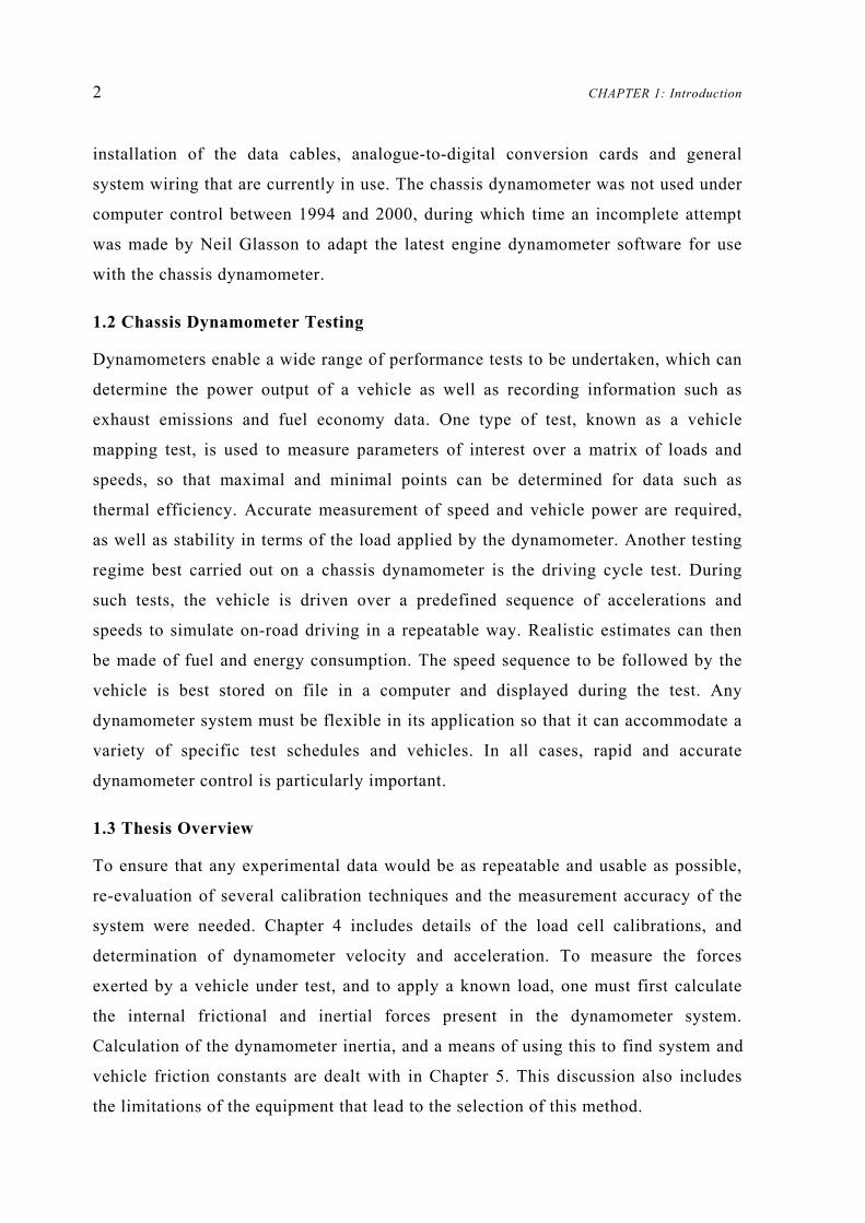
installation of the data cables, analogue-to-digital conversion cards and general
system wiring that are currently in use. The chassis dynamometer was not used under
computer control between 1994 and 2000, during which time an incomplete attempt
was made by Neil Glasson to adapt the latest engine dynamometer software for use
with the chassis dynamometer.
1.2 Chassis Dynamometer Testing
Dynamometers enable a wide range of performance tests to be undertaken, which can
determine the power output of a vehicle as well as recording information such as
exhaust emissions and fuel economy data. One type of test, known as a vehicle
mapping test, is used to measure parameters of interest over a matrix of loads and
speeds, so that maximal and minimal points can be determined for data such as
thermal efficiency. Accurate measurement of speed and vehicle power are required,
as well as stability in terms of the load applied by the dynamometer. Another testing
regime best carried out on a chassis dynamometer is the driving cycle test. During
such tests, the vehicle is driven over a predefined sequence of accelerations and
speeds to simulate on-road driving in a repeatable way. Realistic estimates can then
be made of fuel and energy consumption. The speed sequence to be followed by the
vehicle is best stored on file in a computer and displayed during the test. Any
dynamometer system must be flexible in its application so that it can accommodate a
variety of specific test schedules and vehicles. In all cases, rapid and accurate
dynamometer control is particularly important.
1.3 Thesis Overview
To ensure that any experimental data would be as repeatable and usable as possible,
re-evaluation of several calibration techniques and the measurement accuracy of the
system were needed. Chapter 4 includes details of the load cell calibrations, and
determination of dynamometer velocity and acceleration. To measure the forces
exerted by a vehicle under test, and to apply a known load, one must first calculate
the internal frictional and inertial forces present in the dynamometer system.
Calculation of the dynamometer inertia, and a means of using this to find system and
vehicle friction constants are dealt with in Chapter 5. This discussion also includes
the limitations of the equipment that lead to the selection of this method.

1.3 Thesis Overview 3
The majority of effort on this project was devoted to the presentation of an efficient
and simple computer user interface. To ensure its continued use, it was important that
this program should appear and operate in a familiar way. During any test, a large
number of options are available to the user, from dynamometer and vehicle settings
to the test configuration and duration. As well as presenting the user with these initial
options, the dynamometer control program must also handle the physical running of
the tests, including hardware switching and outputs, A/D data sampling, and on-
screen feedback of test parameters and progress. Chapter 6 contains specifics of the
programming tasks undertaken and the resulting software system.
The repeatability of tests carried out on a chassis dynamometer enables a comparison
between two or more different vehicles undergoing the same test, or a single vehicle
with its configuration altered. For example, the performance of after-market fuel
additives can be determined in a series of trials with and without the product.
Analysis of test data is best made in graphical form, and a versatile results display
program was desired for use with the chassis dynamometer. Ideally, test results
should be able to be plotted quickly and easily, with the capacity to display one or
more test runs on the same axis for the purpose of comparison. The calculation and
prediction of vehicle energy consumption—particularly during a driving cycle run—
is also of interest, and may be used to determine the relative effect of variable cycle
parameters such as the vehicle friction coefficients. Energy consumption modelling
and data graphing software are detailed in Chapter 7. Graphical outputs have been
used to display the results of a series of proving tests that were carried out as part of
the system recommissioning. The response and repeatability of the system as a whole
have been documented in Chapter 8 so that potential improvements can be identified
and to put experimental results in perspective with regards to accuracy and precision.
The purpose of this project was to prepare the University of Canterbury chassis
dynamometer and its accompanying software for use by students of the University as
well as outside parties for the purpose of vehicle testing. Several improvements have
been identified in Chapter 9 that would increase the usefulness of the system as a
whole, and these may form the basis of future student projects at Canterbury.

CHAPTER 2:
The University of Canterbury Chassis Dynamometer
2.1 Common System Configurations
All chassis dynamometers have several key features in common. Most importantly, a
means of absorbing the power output from the test vehicle’s engine is needed to
allow different loads to be applied for a variety of testing procedures. Energy is
transmitted to this power absorber via a direct connection to the vehicle’s wheel
hubs, or through a set of rollers, which are rotated by the wheels of the test vehicle.
Flywheels and/or a motoring capability may also be included if vehicle inertia is to
be simulated. Descriptions of inertia simulation and the modelling of various vehicle
forces are included in Chapter 3. Systems that incorporate a set of large rollers (one
roller for each driven wheel) are more common in applications requiring long term
running of the vehicle, in which tyre overheating can occur. Hub dynamometers are
best suited to engine tuning applications which demand rapid response and minimal
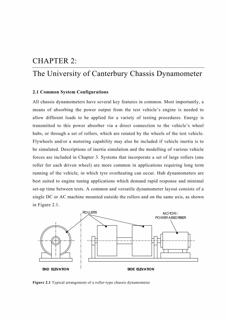
set-up time between tests. A common and versatile dynamometer layout consists of a
single DC or AC machine mounted outside the rollers and on the same axis, as shown
in Figure 2.1.
Figure 2.1 Typical arrangement of a roller-type chassis dynamometer
END ELEVATION SIDE ELEVATION
ROLLERS MOTOR / POWER ABSORBER

6 CHAPTER 2: The University of Canterbury Chassis Dynamometer
Output power is most commonly absorbed by hydraulic or electric machines—also
known as dynamometers—which dissipate power either as heat or electrical energy.
A single unit that can perform both motoring (power output) and generating (power
absorption) functions is a common feature in commercially available chassis
dynamometers.
All but the simplest of garage tuning dynamometers include the capacity to measure
the equivalent road speed and tractive force applied at the vehicle’s wheels. Chassis
dynamometers for in-depth driving cycle and vehicle mapping tests customarily
incorporate many different measuring devices, which are sampled and recorded by a
computer-controlled data acquisition system. Common features of interest during a
dynamometer test include the exhaust emissions (such as CO, CO2, NOX and unburnt
hydrocarbons), vehicle cooling water and oil temperatures, and of course tractive
force and power output. Fuel consumption and air inlet flowrates may also be
recorded for combustion powered vehicles, and these often require adjustment to the
standard engine intake equipment. Where the system is controlled by a computer,
processing power and user interfaces vary greatly. The simplest forms may consist
only of a data logging function which saves information for later viewing, while
more sophisticated systems incorporate digital control of the dynamometer, prompts
and feedback to the operator, as well as the recording and graphical display of data.
Rates of screen update, data sampling, and control signal output are dependent
mostly upon the processing speed of the control computer and its associated
electronics.
2.2 System Configuration at the University of Canterbury
As mentioned in Chapter 1, the entire chassis dynamometer was transplanted into a
new laboratory in 1994. The new layout of the laboratory and the desire to reuse the
present equipment dictated that the power absorbing shaft be mounted at right angles
to the roller drums. The overall dynamometer system is shown in Figure 2.2 and Plate
2.1. The roller drums are carried on a trunnion-mounted Ford 15C truck axle, with its
differential locked and a ratio of 43:7 (6.14:1). The axle assembly is located laterally
by a Watt linkage lying in a horizontal plane beneath the axle, as shown in Figure
2.3.
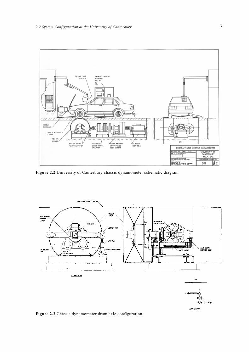
2.2 System Configuration at the University of Canterbury 7
Figure 2.2 University of Canterbury chassis dynamometer schematic diagram
Figure 2.3 Chassis dynamometer drum axle configuration

8 CHAPTER 2: The University of Canterbury Chassis Dynamometer
Plate 2.1 University of Canterbury chassis dynamometer main shaft (from above)
The use of trunnion bearings means that forces applied at the surface of the drums
can be detected by a strain-gauge load cell recording the reaction force of the
assembly on the rigid support stand. To determine the actual force at the drum
surface, the friction and inertia of the drum axle assembly must be taken in to
account. This tractive effort correction is detailed in Section 5.5.
Power is absorbed by a Froude EC50TA Eddy-Current Dynamometer. The supplied
torque and speed measuring equipment of this instrument are used for control
purposes. Originally, the design included a 166 kW D.C. motor-generator set which
ROLLER DRUMS
ELECTRIC MOTOR
POWER ABSORBER
FLYWHEEL

2.2 System Configuration at the University of Canterbury 9
could motor and absorb in both directions. However, this compact regenerative
system was not practical due to a lack of sufficient A.C. mains current capacity. The
water-cooled, disc-type dynamometer was chosen in preference to a hydrokinetic
absorber on the grounds of a superior low-speed torque capacity and a lesser
requirement on the water supply for a given maximum torque rating. The gearing
incorporated in the axle assembly means that the dynamometer operates at a higher
speed and lower torque than if it were connected in a direct fashion to the roller
drums.
A set of flywheels is mounted between the axle and dynamometer to allow inertia
simulation of vehicle masses between 664 kg and 1794 kg. Running through the
centre of the flywheel set is a hollow shaft, which can be rigidly coupled to the main
shaft, or allowed to rotate independently on bearings. Each of the four flywheels sits
on bearings on the outside of the hollow shaft. Flywheels may be engaged to spin
with this shaft—and therefore, with the main shaft—by bolting on the respective
flanges. The discrete inertia intervals that can be achieved by including or omitting
individual flywheels are listed in Appendix A and provide steps of not more than
120 kg over the entire range. While the inertial loads present during acceleration and
deceleration of the roller drums may be accommodated by the eddy-current
dynamometer, the inclusion of flywheels lessens the overall power absorption
requirement. Figure 2.4 shows a schematic of the flywheel assembly.
During calibration and warming up of the system, it is useful to be able to motor the
dynamometer and rollers without the presence of a vehicle. A 26 kW ASEA LAK
180LA D.C. motor has been installed, which is controlled by a 3 phase thyristor
converter with polarity reversing switch gear to enable motoring in both directions. It
was intended that this machine perform additional inertia simulation—particularly
during deceleration—in the original configuration. However, it was found that the
response time and control accuracy were insufficient for this task (see Section 5.2.3)
and that the power absorber and flywheels offered superior inertia approximation
without the use of the electric motor. As shown in Figure 2.2, the components of the
system are connected via universal shafts to accommodate any misalignment.
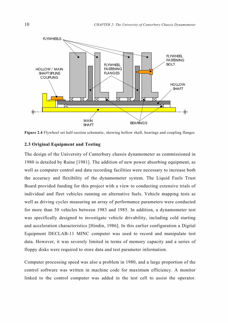
10 CHAPTER 2: The University of Canterbury Chassis Dynamometer
Figure 2.4 Flywheel set half-section schematic, showing hollow shaft, bearings and coupling flanges
2.3 Original Equipment and Testing
The design of the University of Canterbury chassis dynamometer as commissioned in
1980 is detailed by Raine [1981]. The addition of new power absorbing equipment, as
well as computer control and data recording facilities were necessary to increase both
the accuracy and flexibility of the dynamometer system. The Liquid Fuels Trust
Board provided funding for this project with a view to conducting extensive trials of
individual and fleet vehicles running on alternative fuels. Vehicle mapping tests as
well as driving cycles measuring an array of performance parameters were conducted
for more than 30 vehicles between 1983 and 1985. In addition, a dynamometer test
was specifically designed to investigate vehicle drivability, including cold starting
and acceleration characteristics [Hindin, 1986]. In this earlier configuration a Digital
Equipment DECLAB-11 MINC computer was used to record and manipulate test
data. However, it was severely limited in terms of memory capacity and a series of
floppy disks were required to store data and test parameter information.
Computer processing speed was also a problem in 1980, and a large proportion of the
control software was written in machine code for maximum efficiency. A monitor
linked to the control computer was added in the test cell to assist the operator.
FLYWHEELS
FLYWHEEL FASTENING BOLT FLYWHEEL
FASTENINGFLANGES
HOLLOW SHAFT
BEARINGSMAIN SHAFT
HOLLOW / MAIN SHAFT SPLINE COUPLING

2.4 Peripheral System Elements 11
Extended inertia simulation was achieved by means of the flywheel set discussed in
Section 2.2, which was added in 1985.
When extensions to the building required that the chassis dynamometer be relocated,
it was decided that a further computer upgrade would be beneficial. The Froude
dynamometer, ASEA electric motor, flywheel set, and drum/axle assembly have
remained largely the same, with the most important changes being in the control of
the machines and the acquisition of test data. Although the system was not used for
any significant testing between 1994 and 2000, the existing sensors and wiring
remain essentially as they were set up during 1994. The notable exceptions being the
addition of several thermocouples, new electronic filtering circuitry, and the
inclusion of air flowrate, fuel flowrate, and NOX emission meters to the A/D data
sampling capability. The inherent capability of the current hardware has also been
enhanced by the introduction of the current computer program, particularly in regards
to repeatable driving cycle, mapping, and maximum power testing.
2.4 Peripheral System Elements
The current facility at the University of Canterbury includes several features that aid
successful testing, but are not intrinsic parts of the chassis dynamometer system.
Stationary testing of any kind places a high demand on cooling systems for both the
vehicle under test and the dynamometer itself. The Mechanical Engineering chassis
dynamometer laboratory is equipped with a portable fan for cooling of the test
vehicle, while a constant air temperature is maintained by large extractor fans with
associated ducting. This extraction system was designed to remove all the waste heat
from a vehicle supplying a constant wheel power of 200 kW, with a 10ºC rise in
ventilation air temperature. An exhaust extraction fan and duct is also supplied to
remove unwanted contaminants from the laboratory environment. The dynamometer
drum axle and power absorber are both water cooled, and have temperature sensors
which can be monitored in the control room. To anchor the test vehicle, a set of steel
cables and chains are secured to the laboratory floor on purpose-built fastenings. To
assist the driver of the test vehicle, 13-inch repeater monitor linked to the control-
room computer provides visual feedback and allows the operator to set parameters
and view results without leaving the test cell. The monitor and keyboard are mounted

12 CHAPTER 2: The University of Canterbury Chassis Dynamometer
on an adjustable pendant arm, which also services the electrical wiring for several
sensors including the tachometer and vehicle temperature thermocouples.
2.5 Computer and Electronics Specifications
The control computer consists of an AMD-K6/200 processor, 64 Mb RAM, and
4.01 Gb hard drive running Microsoft® Windows 951 on the Mechanical Engineering
network. As mentioned in Section 2.4, a repeater monitor and keyboard are provided
in the test cell and control of the CPU can be switched between this and the control
room equipment. The user interface and test control program was designed to be run
in a DOS environment, and was written using Borland C++ Version 3.12. The overall
appearance is an outcome of the decision to use the Turbo Vision®3 application
framework, which implements a Windows-like appearance and method of navigation.
Additional software has been written using MATLAB® version 5.3.0.10183 (R11)4
for the viewing and presentation of test data. This software is menu-driven, and has
been used to produce the graphs presented in Chapters 7 and 8. All output files
generated by the main program are also suitable for importing into Microsoft Excel®5
for producing tables or further data manipulation.
Up to 16 A/D channels of data input are handled through a PC-LabCard PCL-812PG
data acquisition card with a PCLD-889 daughter board providing an additional 16
multiplexed channels, which are used mainly for thermocouple temperature sensors.
The computer is also programmed to send digital switching commands and variable
voltage D/A signals via the PCL-812PG. Switching commands include the
dynamometer and electric motor operation modes (via a PCLD-785 digital output
board), as well as gain and channel bit-codes for the PCLD-889 multiplexer. The two
D/A channels may be used to control the motor output power under speed or torque
control, and the power absorber by means of speed, torque, or a power law control. A
1 Copyright Microsoft Corporation 2 Copyright 1990, 1992 Borland International 3 Copyright 1991, Borland International 4 Copyright 1984–1999 The Mathworks, Inc 5 Copyright Microsoft Corporation
2.5 Computer and Electronics Specifications 13
differential-input low-pass filter circuit board designed and constructed at the
University of Canterbury is used to decrease the signal noise before voltages are
received by the A/D card. Various equipment modes, as well the state of the air and
water supplies, are also monitored by the PCL-812PG via a PCLD-782 opto-isolated
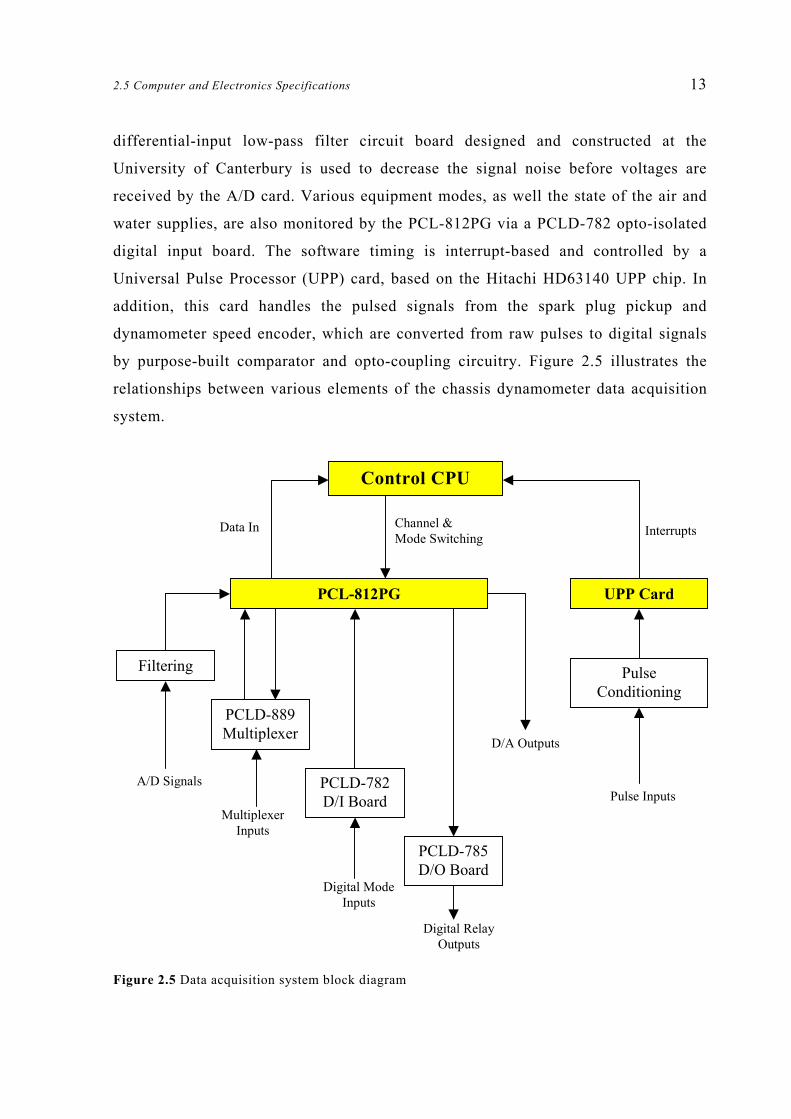
digital input board. The software timing is interrupt-based and controlled by a
Universal Pulse Processor (UPP) card, based on the Hitachi HD63140 UPP chip. In
addition, this card handles the pulsed signals from the spark plug pickup and
dynamometer speed encoder, which are converted from raw pulses to digital signals
by purpose-built comparator and opto-coupling circuitry. Figure 2.5 illustrates the
relationships between various elements of the chassis dynamometer data acquisition
system.
Figure 2.5 Data acquisition system block diagram
Control CPU
PCL-812PG
Pulse Conditioning
UPP Card
Filtering
PCLD-889 Multiplexer
Pulse Inputs
Channel & Mode Switching
Data In
Multiplexer Inputs
A/D Signals PCLD-782D/I Board
Digital Relay Outputs
Digital Mode Inputs
PCLD-785D/O Board
Interrupts
D/A Outputs

14 CHAPTER 2: The University of Canterbury Chassis Dynamometer
The Plate 2.2 shows the arrangement of the various circuit boards located in the
automotive control room. Note that the UPP card and PCL-812PG are mounted in
ISA slots inside the PC and so are not visible.
Plate 2.2 Control room electronics cabinet
2.5.1 Measured Parameters
In the main data acquisition program, inputs are recognised in several ways,
including: voltages converted directly by the PCL-812PG A/D card, voltages
received by the PCL-812PG via the PCLD-889 multiplexer, and external inputs that
do not fall into either of these two categories. The multiplexer has 16 available
channels in addition to a cold junction compensation (CJC) signal. Of these, six are
currently in use. On the PCL-812PG, one channel is used to access the multiplexing
channels and another the CJC channel. Of the remaining 14 channels, seven are
PCLD-782 D/I BOARD
PULSE CONDITIONING CIRCUITS
DIFFERENTIAL INPUT FILTER BOARD
PCLD-889 MULTIPLEXER
PCLD-785 D/O RELAY BOARD

2.5 Computer and Electronics Specifications 15
currently in use (including a spare channel kept free for miscellaneous voltage
testing). There is no express limit on the number of external inputs, but at this point
velocity and engine speed are the only inputs not read through the PCL-812PG. Table
2.1 summarises the measured parameters.
Table 2.1 Channel assignment table
During a chassis dynamometer driving cycle or mapping test, demand signals from
the computer are sent to the Froude dynamometer at the rate of 10 Hz . D/A output
signals may be used to control the machine in any of its three modes of operation;
constant speed, constant torque, or ‘power law’. However, the power law mode—in
which torque varies with speed—was not used for any of the testing detailed in
Chapter 8, and is not discussed any further in this thesis. Constant speed mode was
used to maintain the set points during mapping tests, while driving cycle and
Channel Parameter Units Signal
External Inputs: UPP card
Speed kph 0–5500Hz
RPM RPM 0–350Hz
PCL-812PG
0 Test Channel V ±10V
1 PA Torque Nm 0–10V
2 Tractive Effort N ±5V
3 Motor Torque Nm ±2.5V
4 Fuel Flowrate gm/s 0–5V
5 Air Flowrate gm/s 4–20mA
6 NOX Concentration ppm 0–5V
8 CJC (thermocouple compensation) V ±1.25V
9 Multiplexer V from PCLD-889
PCLD-889 Daughter Board
0 Ambient Air Temp. °C ±2.5mV
1 Drum Axle Oil Temp. °C ±5mV
2 Vehicle Water Temp. °C ±10mV
3 Vehicle Oil Temp. °C ±10mV
4 Spare Thermocouple °C ±10mV
10 Ambient Air Pressure mb 0–1999mV

16 CHAPTER 2: The University of Canterbury Chassis Dynamometer
maximum power runs were best controlled with constant torque. While a consistent
demand may be sent from the computer, the 3-term analogue controller built in to the
dynamometer is continuously updating the actual electric field that defines the
absorbed torque. During a driving cycle test, which requires a continuously varying
load on the vehicle, the demand torque may be varying rapidly. From the software
point of view, this demand sequence consists of a series of open-loop commands,
with each new command being acted on by the closed-loop analogue controller. The
same may be said of the motor control. Although it is not commonly used during
quantitative tests, the ASEA electric motor has its own controller, which may be
provided with a series of constant demands by the computer program.
2.6 Overview of Software Functionality
A brief outline of the capability and scope of the main C++ computer program is
included here. A more detailed description, including the specific programming
challenges and complete functionality, can be found in Chapter 6.
2.6.1 Preliminary Details
The main program can be operated either using a mouse and keyboard, or keystrokes
only. A series of pull-down menus present the various options for calibration, file
handling, and testing routines. Numerical inputs can be selected and typed in, and the
results confirmed in a familiar way by the use of ‘OK’ or ‘Cancel’ buttons. Each
vehicle to be tested has its own data file, which contains the make and model as well
as data such as mass and on-road frictional resistance. Vehicle mass is important in
determining which of the selectable flywheels are to be included to most closely
match the on-road inertia. Once a vehicle and configuration file have been chosen,
several testing options may be selected.
Before meaningful measurements can be made, it is important to ensure that all the
measurement devices are correctly calibrated against known values. The program
includes a simple, general-purpose routine that prompts the user for an independently
measured value, then records and compares the A/D input from the appropriate pre-
selected channel. A mathematical curve-fit is generated for each set of data, which
can then be used to calculate the physical value, given the A/D voltage input during

2.6 Overview of Software Functionality 17
testing. These calibration coefficients (often taking the linear form of a gradient and
an offset) can be entered by the user into a configuration file for future use. The
calibration data capture procedure and on-screen display is discussed further in
Section 6.5.4.
Routines are also included to account for day-to-day variations in system friction and
the zero value of the load cells, with step-by-step instructions given on screen.
Section 4.3 discusses the limitations of these load cells, and the rationale behind the
inclusion of a re-zeroing procedure. Friction calibration is accomplished using a
series of dynamometer coastdowns, which are introduced in Chapter 5.
2.6.2 Routines for Running a Vehicle
Several modes of operation were incorporated to allow a wide variety of flexible
testing programs to be carried out on the University of Canterbury chassis
dynamometer. Each routine requires that a known force be applied by the
dynamometer to the wheels of the test vehicle. By analysing the equations of motion
of the system (see Chapter 3) the power absorber demand required to achieve a given
tractive force—particularly under road load simulation—may be calculated. In this
so-called road load simulation mode, the driver can accelerate and decelerate at will
while the computer sends a load demand to the eddy-current dynamometer such that
the forces experienced at the wheels of the vehicle are equal to those on a vehicle
undergoing similar speeds and accelerations on the road. The specific routines
mentioned below, and the underlying program structure, are discussed in more detail
in Chapter 6.
The ‘Warm Up’ routine is available to prepare the chassis dynamometer and vehicle
for testing by running at constant speed, or under an approximate road load until the
lubricating oil and all bearing surfaces have stabilised in terms of temperature and
frictional attributes.
The ‘Road Load Driving’ option allows running of a vehicle under road load
conditions, while all the measured parameters are shown on the screen—updated at
the rate of 5 Hz—and can be saved to a pre-selected file at the touch of a button.

18 CHAPTER 2: The University of Canterbury Chassis Dynamometer
‘Manual Control’ mode is similar in appearance to ‘Road Load Driving’, but allows
the operator to select constant speed and torque demands for both the motor and the
dynamometer. This mode is useful for performing maximum power tests in which full
throttle is applied and the vehicle is allowed to accelerate over a set speed range,
while measuring—in particular—the power output by the vehicle. Such tests are
invaluable in tuning work where small changes in settings on the engine are not
easily discerned except by comparison of the resulting torque curves.
The entire performance envelope of a vehicle may be investigated by carrying out a
‘Mapping Test’. By running at a series of predetermined speeds and dynamometer
loads, a map of each measured parameter can be built up which shows not only the
peak numerical value, but also the optimal running conditions in terms of speed and
load. Common parameters of interest in this type of test include fuel consumption,
brake thermal efficiency, and the proportions of CO, CO2, HC and NOX in a vehicle’s
exhaust. Coloured contour plots of each parameter can be produced using the
MATLAB routines detailed in Chapter 7.
Another common method of comparing vehicle performance is the ‘Driving Cycle’
test. Many different cycles have been created which attempt to reproduce common
driving patterns either in an urban environment or on the open road. The speed and
duration of these simulated trips depend on the driving habits and traffic conditions
in the area of interest. On the chassis dynamometer, a driving cycle file contains the
desired speed at each one-second interval for the entire test. This speed is reproduced
graphically in the form of a scrolling line, which the driver of the vehicle under test
attempts to follow by accelerating and changing gears as one would on the road. The
power absorber is sent updating demands at 10 Hz to simulate the road load forces as
closely as possible. Again, all the parameters of interest are recorded and saved to a
file, which can be used to find the maximum point, the average, or to produce a plot
for comparisons. Accidental deviations from the desired speed are inevitable when a
human driver controls the test vehicle. However, a record is kept of the total number
of discrepancies and the test may be aborted if the schedule is not maintained within
the allowable limits. A MATLAB routine (see Section 7.2) has also been designed to
compare the total energy consumed in terms of power output at each instant with that

2.7 Comparative Performance of the University of Canterbury Chassis Dynamometer 19
calculated by fuel energy consumption and the hypothetical case of the vehicle
exactly following the demand speed throughout. Driving cycle tests are most
commonly used to compare the fuel consumption and exhaust emissions of vehicles
under local on-road conditions in a repeatable and quantifiable way.
2.7 Comparative Performance of the University of Canterbury Chassis Dynamometer
In terms of power absorbing capacity and maximum speed, the University of
Canterbury dynamometer compares favourably to commercially available chassis
dynamometers at the time of writing. Several commercial dynamometers have been
investigated and a summary of various performance specifications has been included
in Appendix B. Comparable roller-type chassis dynamometers produced by Schneck
and Froude Consine have similar drum diameters, but are designed to measure a
lower tractive effort range than the University of Canterbury facility. However, due
to the considerable age of the machinery detailed in this thesis, load response and
stability are below industry standard. A faster data sampling rate (which could be
facilitated by greater computer processing power) may also be desirable to improve
the quality of results using the chassis dynamometer. The testing facility and its
associated equipment such as exhaust and cooling fans provide an excellent
laboratory environment and capacity exists for significant extension of the sampled
data channels.


CHAPTER 3:
Equations of Motion
In order to apply a known dynamometer load, the characteristics of the system and
how these relate to the vehicle under test must be determined. The vehicle power
output is measured as a force and speed at the road surface. This force is known as
the tractive effort and is commonly measured on a roller-type dynamometer by a load
cell indirectly connected to the rollers. For steady state testing, it is sufficient to
know the frictional losses of the system so that the power absorber can combine with
the friction to apply a given load at a given speed. However, if measurements are to
be made during speed transients—as in a driving cycle test—it is necessary to include
inertial effects.
3.1 Vehicle Tractive Effort
A vehicle in motion is subject to various gravitational, frictional, and inertial loads.
The tractive effort to overcome these resistances, FV applied at the surface of the road
wheels is given by:
( ) 221 2
1 AvρCdtdvmθgmvCCgmF DVeqV
nRRVV +
+++= sin (3-1)
See following page for notation.
ROLLING RESISTANCE
GRAVITATIONAL + INERTIAL RESISTANCE
AIR RESISTANCE

22 CHAPTER 3: Equations of Motion
Where: v = linear vehicle velocity (m/s)
dtdv = linear vehicle acceleration (m/s2)
θ = road gradient
ρ = air density
n = index dependent on design of tyre and running gear
mVeq = total equivalent mass (kg) = mV + equivalent mass of rotational
components
Other notation as per Nomenclature section.
Rolling resistance depends largely on tyre design and inflation pressure, as well as
the condition of the road surface. CR values vary significantly in the early stages of a
journey as the tyres and running gear warm up [Burke et al., 1957]. CR1 may range
between 0.01 and about 0.04 [Wheeler, 1963], while the CR2vn term is dependent
upon tyre design and temperature, and becomes significant at higher speeds (above
90 kph)[Elliot et al., 1971]. These values are quoted for a warmed up vehicle on a
straight road, and frictional constants under cornering are not usually included in the
tractive effort model. Note that these coefficients are based on somewhat dated
references. Any new chassis dynamometer research should utilise more recent
literature to incorporate the latest tyre designs and resulting frictional performance.
The aerodynamic drag coefficient CD depends primarily upon the body shape of the
vehicle, as well as the air flow through the radiator and over the external fittings.
Typical CD values for road-going passenger cars at the time of writing were 0.25–
0.35 in still air.
In cases where the frictional characteristics of a vehicle are determined
experimentally, the individual magnitudes of these constants are not necessarily
distinguishable and the tractive effort equation is simplified to:
2210 vfvff
dtdvmF VVVVeqV +++= (3-2)
Where: f0V, f1V, f2V = combined vehicle friction constants

3.2 Chassis Dynamometer Equations of Motion 23
The gravitational forces brought about by an incline in the road surface may be
modelled on the dynamometer, and although capability exists for such a simulation,
road gradient effects were not generally incorporated in dynamometer tests conducted
at the University of Canterbury. Also, the vehicle mass must include the inertial
influence of its rotational parts such as the engine flywheel and road wheels, which
act to increase the magnitude of the tractive force required for changes in speed. This
rotational component is added to the actual vehicle mass (for mVeq dv/dt calculations)
and can be either measured experimentally or approximated. A common
approximation is:
0351.×= VVeq mm (3-3)
This approximation may not hold for a wide variety of vehicle types. Equation 3-3 is
used throughout this thesis, although more recent research may indicate a different
factor or rotational inertia correction.
3.2 Chassis Dynamometer Equations of Motion
The free-body diagram Figure 3.1 shows all the external forces acting on the chassis
dynamometer during motion. It is helpful to express each torque acting on the shaft
in terms of the equivalent force at the drum surface. This conversion can be made
with the use of the axle differential ratio (43:7) and the roller drum radius (0.6 m).
An example is provided for the case of the eddy-current dynamometer
electromagnetic force.
×=
radiusdrumratiodiffTF dede (3-4)
Where: Tde = Electromagnetic torque at eddy-current dynamometer
Note that the electric motor always applies a force in the direction of motion, while
the dynamometer force and frictional forces are in the opposite direction to the drum
velocity.

24 CHAPTER 3: Equations of Motion
The rotational inertia of each component is also expressed in terms of the roller
drums. The equivalent mass if the inertia was concentrated at the drum surface is
found as follows:
( )2radiusdrum
Imeq = (3-5)
Where: I = rotational inertia of component
Rotation of the chassis dynamometer in a positive direction is arbitrarily defined as
being in the direction shown in Figure 3.1. Velocity and acceleration are as indicated
at the rollers, and the main shaft rotates in such a way that the top of the flywheels
move into the page. Under a positive force from the test vehicle, the tractive effort
load cell is in compression, indicating a positive tractive force. The power absorber
applies an opposing force, and the electric motor exerts a force in the same direction
as the shaft rotation, both of which read positive on their respective load cells.
Figure 3.1 Chassis dynamometer free-body diagram
Where: v = velocity at drum surface (m/s)
v& = acceleration at drum surface (m/s2)
Fv = vehicle tractive force (N)
Other notation as per Nomenclature section
Fv
Fmf Fme
Fdrf Fdra
Fff Fde
Fsf
Fdf
mdr (ROLLER DRUMS)
ms (SHAFT)
mm (MOTOR)
md (DYNO)
mff (FLYWHEELS)
v, v ˙
T.E. LOAD CELL MOTOR LOAD ARMDYNO LOAD CELL
VEHICLE ON ROLLERS

3.3 Combined Tractive Effort 25
The overall equation can be stated as per Equation 3-6:
( ) ( ) ( ) ( ) ( ) ( )sfmffddeffdradrfmev FFFFFFFFF −−+−−+−+
( )vmmmmm smdffdr &++++= (3-6)
Or, grouping the mass terms together and approximating the total friction force as a
quadratic in relation to speed:
( ) vmvfvffFFF cdddddemev &=++−−+ 2210 (3-7)
Where: mcd = combined chassis dynamometer equivalent mass (kg)
This equation may be stated in terms of the tractive force from the vehicle, which is
equal to the reaction force from the chassis dynamometer as a whole:
( )2210 vfvffFFvmF dddmedecdv +++−+= & (3-8)
The torque reading given by each of the three load cells includes a friction and inertia
component, depending on the individual configurations. Each of these load cell
configurations is subject to friction in the trunnion bearings on which they are
supported. This friction acts in opposition to the measured force, but is not
experienced by the load cell, and therefore cannot be measured or included in the
equations of motion. Section 4.3 contains a further description of the load cell
dynamics and calibration techniques.
3.3 Combined Tractive Effort
To simulate the appropriate vehicle road load at any given speed and acceleration, the
characteristics of both the chassis dynamometer and the vehicle under test must be
known and combined. The forces experienced by a vehicle on the road (as per
Equation 3-2) are matched by the forces experienced by the same vehicle on the
dynamometer. While mounted on the chassis dynamometer, the vehicle is no longer
subject to the air resistance component of Equation 3-1 or the rotational inertia of the
non-driven wheels. This lesser inertia is generally ignored or included in the
approximation of mVeq. To accommodate the differing friction values, a test may be

26 CHAPTER 3: Equations of Motion
carried out to determine the frictional characteristics of the dynamometer and test
vehicle combined, which are then included in the tractive forces applied by the
dynamometer for the purposes of Equation 3-8.
( ) ( ) medeVdVdVdcdVVVVeq FFvfvffdtdvmvfvff
dtdvm −++++=+++ 2
2102
210 (3-9)
Where f0Vd, f1Vd, f2Vd = frictional coefficients of vehicle on the dynamometer
In general, the only parameters that can be continuously varied during a test cycle are
the power absorber force and the motoring force. We require a formulation that can
be solved for these variable parameters. The net output of each device is the
combination of electromagnetic force and internal friction, which is set by the
respective controllers and measured by the load cells (see Section 5.1). Thus, we
modify the coefficients f0Vd etc. to exclude the friction from within the powered
devices. During chassis dynamometer operation the modified Equation 3-9 is
constantly solved to determine the necessary combined net demand force (Fnet).
( ) ( ) ( ) ( ) 2221100 vffvffff
dtdvmmF VdVVdVVdVcdVeqnet ′−+′−+′−+−= (3-10)
Where: Fnet = Fdyno – Fmotor
Fdyno = power absorber control demand (N)
Fmotor = electric motor control demand (N)
VdVdVd fff 210 ′′′ ,, = combined friction coefficients of chassis dynamometer and
vehicle, less the internal friction of the electromagnetic devices
In reality, the magnitudes of these altered fVd coefficients are determined by whether
or not the power absorber or electric motor were operating during the friction
calibration (see Section 5.1). The inertial force applied by the chassis dynamometer
to account for the mass difference (mVeq – md) is minimised by the use of the flywheel
set, as detailed in Section 2.2. The various flywheel combinations ensure that for
FORCES ACTING ON = FORCES ACTING ON VEHICLE ON ROAD VEHICLE ON DYNAMOMETER

3.3 Combined Tractive Effort 27
vehicle masses between 604 kg and 1854 kg the absolute value of the mass difference
need not be greater than 60 kg (see Appendix A).
For vehicle tests other than driving cycles, a constant tractive effort is often desired,
as opposed to a continuously varying road load. Applying a set tractive force at the
drum surface does not require knowledge of the vehicle characteristics, and
Equation 3-8 is solved for the net demand force Fnet. Constant load tests (for
example, vehicle mapping) are almost always carried out at a series of constant
speeds (dv/dt = 0), further simplifying the load equation to:
( )2210 vfvffFF dddVnet ′+′+′−= (3-11)
Again: ddd fff 210 ′′′ ,, refer to friction coefficients of the chassis dynamometer not
including the contribution from the powered device

CHAPTER 4:
Details of Selected Instrumentation
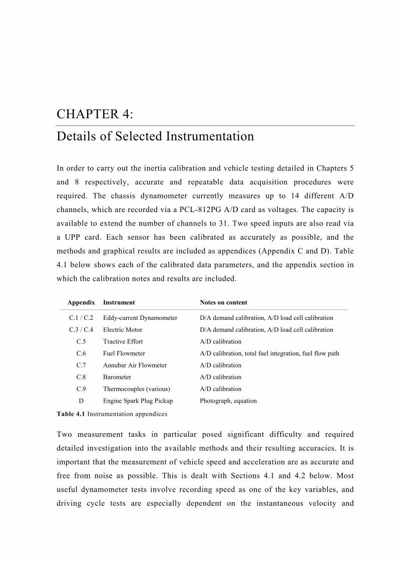
In order to carry out the inertia calibration and vehicle testing detailed in Chapters 5
and 8 respectively, accurate and repeatable data acquisition procedures were
required. The chassis dynamometer currently measures up to 14 different A/D
channels, which are recorded via a PCL-812PG A/D card as voltages. The capacity is
available to extend the number of channels to 31. Two speed inputs are also read via
a UPP card. Each sensor has been calibrated as accurately as possible, and the
methods and graphical results are included as appendices (Appendix C and D). Table
4.1 below shows each of the calibrated data parameters, and the appendix section in
which the calibration notes and results are included.
Table 4.1 Instrumentation appendices
Two measurement tasks in particular posed significant difficulty and required
detailed investigation into the available methods and their resulting accuracies. It is
important that the measurement of vehicle speed and acceleration are as accurate and
free from noise as possible. This is dealt with Sections 4.1 and 4.2 below. Most
useful dynamometer tests involve recording speed as one of the key variables, and
driving cycle tests are especially dependent on the instantaneous velocity and
Appendix Instrument Notes on content
C.1 / C.2 Eddy-current Dynamometer D/A demand calibration, A/D load cell calibration
C.3 / C.4 Electric Motor D/A demand calibration, A/D load cell calibration
C.5 Tractive Effort A/D calibration
C.6 Fuel Flowmeter A/D calibration, total fuel integration, fuel flow path
C.7 Annubar Air Flowmeter A/D calibration
C.8 Barometer A/D calibration
C.9 Thermocouples (various) A/D calibration
D Engine Spark Plug Pickup Photograph, equation

30 CHAPTER 4: Details of Selected Instrumentation
acceleration of the test vehicle. In the absence of a dedicated accelerometer, it is
necessary to calculate acceleration as the change in velocity with time—that is, to
differentiate. Section 4.3 details the calibration and software techniques used to
ensure accurate load cell measurements, given the existing hardware and geometry.
In the case of the power absorber and drum axle load cells, calibration techniques
were formulated to accommodate the hysteresis and temperature-dependence of these
devices.
4.1 Measurement of Velocity
As mentioned above, the measured velocity is a valuable test parameter, and is also
used to calculate the instantaneous acceleration. As with most digitally recorded data,
electrical noise and instrument inaccuracies are exacerbated when the signal is
differentiated, as small, rapid fluctuations translate to large variations. For this
reason, it was necessary to first find the most accurate and noise-free method of
measuring the raw vehicle velocity, then to apply the filtering and acceleration
calculations most appropriate for the chassis dynamometer system as a whole (see
Section 4.2).
4.1.1 Frequency-to-Voltage Conversion
A previous chassis dynamometer configuration at the University of Canterbury
recorded the roller rotational speed (and hence, test vehicle velocity) indirectly using
a magnetic encoder included in the eddy-current dynamometer. The dynamometer
includes a toothed wheel, which rotates with the main shaft, setting up a magnetic
field of varying intensity as the teeth pass between a pair of magnets. These pulses
are converted to electrical pulses, which in turn are converted to a voltage by the
dynamometer circuitry. The output of this frequency-to-voltage conversion is used by
the dynamometer when in speed-control mode, and can also be measured by the
computer. The advantage of this system was that the voltage signal could be easily
recorded using the existing A/D board. The major difficulty in using the voltage from
the dynamometer was that the signal was subject to the significant noise experienced
by the system, especially within the power absorber circuitry. Plots of the frequency-
to-voltage signal under normal operating conditions are in Figure 4.1. A constant
speed of approximately 10 kph was maintained by the electric motor while under a

4.1 Measurement of Velocity 31
constant loading of 100 Nm from the eddy-current dynamometer. This arrangement
was chosen to roughly approximate conditions during testing, while minimising
additional vibrations that may have arisen at higher speeds.
0 0.5 1 1.5 2 2.5 3 3.5 4 4.5 59.6
9.7
9.8
9.9
10
10.1
10.2
10.3
10.4
10.5
10.6
Time (sec)
Vel
ocity
(kph
)
Figure 4.1 Velocity signal generated by dynamometer frequency-to-voltage converter
It can be seen the noise present in the voltage output is of the order of ±0.4 kph,
which was considered significant, especially in regards to its eventual conversion to
acceleration. By measuring an encoder output more directly, it was hoped that a large
portion of this electrical noise could be avoided.
4.1.2 Rotary Encoders
Two rotary shaft encoders were available to measure the chassis dynamometer speed:
the built-in magnetic encoder used by the eddy-current dynamometer, and an optical
device mounted on the drum axle. Both signals were recorded using a UPP card
constructed by University of Canterbury technicians, which performs digital
switching on voltage pulses. Both encoders also required additional signal
conditioning circuitry for use with the UPP card. All interrupt handling software was
written and modified for use with the chassis dynamometer by Dr Andrew Cree.
4.1.2.1 Drum Axle Encoder
Given that the system is torsionally flexible to some degree, a velocity reading taken
at the drum axle (which is effectively at the road surface) is more accurate in relation
to a vehicle under test. However, if this drum speed were used to determine the
dynamometer loading, significant inertia—and corresponding rotational lag—
between the speed reading and the power-absorber could potentially lead to a degree
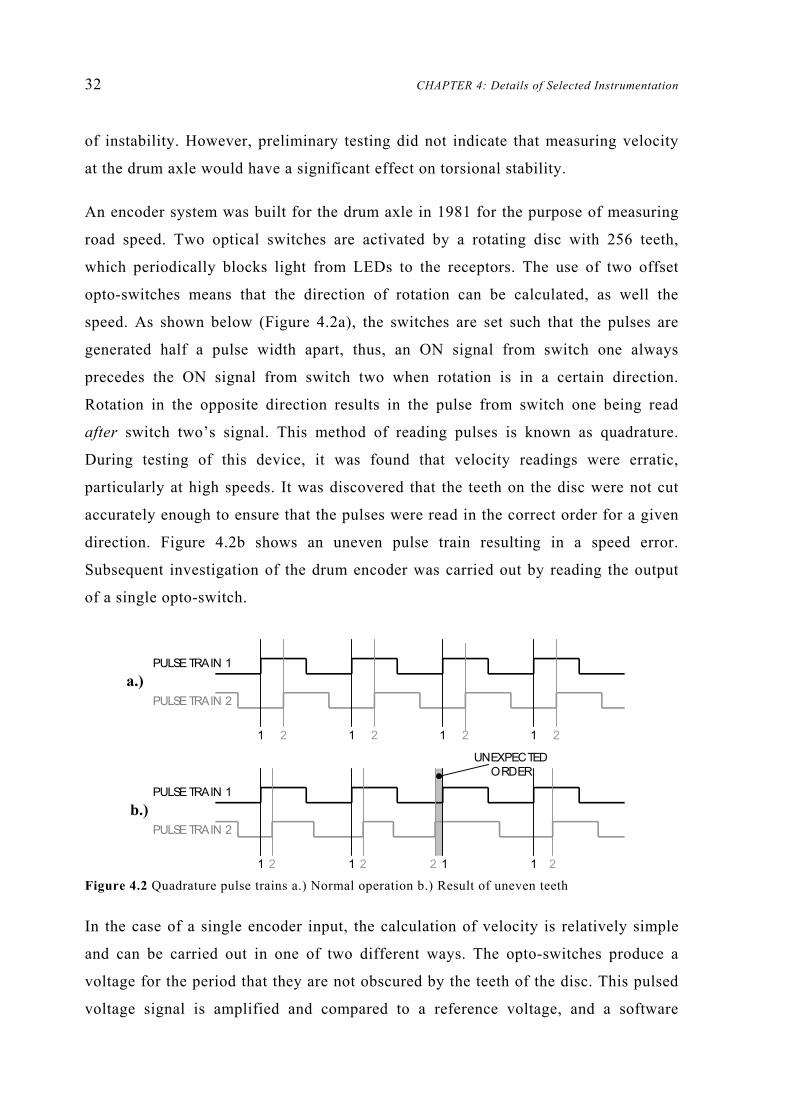
32 CHAPTER 4: Details of Selected Instrumentation
of instability. However, preliminary testing did not indicate that measuring velocity
at the drum axle would have a significant effect on torsional stability.
An encoder system was built for the drum axle in 1981 for the purpose of measuring
road speed. Two optical switches are activated by a rotating disc with 256 teeth,
which periodically blocks light from LEDs to the receptors. The use of two offset
opto-switches means that the direction of rotation can be calculated, as well the
speed. As shown below (Figure 4.2a), the switches are set such that the pulses are
generated half a pulse width apart, thus, an ON signal from switch one always
precedes the ON signal from switch two when rotation is in a certain direction.
Rotation in the opposite direction results in the pulse from switch one being read
after switch two’s signal. This method of reading pulses is known as quadrature.
During testing of this device, it was found that velocity readings were erratic,
particularly at high speeds. It was discovered that the teeth on the disc were not cut
accurately enough to ensure that the pulses were read in the correct order for a given
direction. Figure 4.2b shows an uneven pulse train resulting in a speed error.
Subsequent investigation of the drum encoder was carried out by reading the output
of a single opto-switch.
Figure 4.2 Quadrature pulse trains a.) Normal operation b.) Result of uneven teeth
In the case of a single encoder input, the calculation of velocity is relatively simple
and can be carried out in one of two different ways. The opto-switches produce a
voltage for the period that they are not obscured by the teeth of the disc. This pulsed
voltage signal is amplified and compared to a reference voltage, and a software
PULSE TRAIN 1
PULSE TRAIN 2
PULSE TRAIN 1
PULSE TRAIN 2
2 2 2 2
2 2 2 2
1 1 1 1
1 1 1 1
UNEXPECTED ORDER
a.)
b.)

4.1 Measurement of Velocity 33
interrupt is generated when the reference voltage is exceeded. The spacing between
the teeth is fixed and represents a certain angle of rotation of the shaft, so the
calculation of rotational velocity is a matter of measuring the rotation (in terms of
interrupts) and the elapsed time (using the UPP card timer). Either the number of
interrupts registered in a given time period is counted, or the duration between
successive interrupts is timed. The former method is referred to here as counting
(Equation 4-1), and the latter as timing (Equation 4-2).
( )( )
( )intervaltimeFixedpulseperAnglepulsesofNumber
Tn
dtd
f
pp ===θθθ& (4-1)
( )
( )( )cycleclockperTimecyclesclockofNumberpulseperAngle
Tndtd
cc
p ===θθθ& (4-2)
Included below is a plot of the speed signal under a constant dynamometer torque as
is shown in Figure 4.1. Velocity has been calculated by the counting the pulses in
each 0.1s interval. Note the difference in vertical-axis scale between Figures 4.1 and
4.3.
0 0.5 1 1.5 2 2.5 3 3.5 4 4.5 59.75
9.8
9.85
9.9
9.95
10
10.05
10.1
10.15
Time (sec)
Vel
ocity
(kph
)
Figure 4.3 Velocity signal generated by counting drum encoder pulses at 10 Hz
The errors due to unevenness of the encoder teeth have an effect on the velocity
whether one is counting pulses or timing them. The magnitude of this error depends
on the rotational speed, and of course the physical difference in the width of adjacent
teeth. The relative errors as a result of speed and method of calculation are addressed
in Section 4.1.3. Ordinarily during velocity measurement by timing, one might record

34 CHAPTER 4: Details of Selected Instrumentation
several time intervals and average them to arrive at the rotational speed. However, by
recording the time interval between every pulse, the relative angular widths of the
teeth can be found (θ = average rotational speed × time between pulses). Figure 4.4
represents each width (i.e. the tooth width plus the width of the gap before the next
tooth) on the radial axis and its position around the wheel’s perimeter in the
circumferential direction. Two consecutive plots are overlaid (one light and one dark
line), showing excellent repeatability and proving that each spike can be traced to a
specific encoder tooth. The unit on the radial axis is percentage with zero being the
average tooth angle and those angles which are either greater or lesser shown in
proportion.
256360o
==teethofNumber
ncecircumferearoundangleTotalangletoothAverage (4-3)
Thus, the large value shown as +5% at 255º represents a tooth width (including the
adjacent gap) of approximately (360/256)×1.05 = 1.48º. While these figures are not
intended to be highly accurate, they provide a useful relative measure of the encoder
wheel in situ.
30
210
60
240
90
270
120
300
150
330
180
Relative Tooth Width (% ) +5% - 5% +10% -10%
O
O
O
O
O
O
O
O
O
O
O
Angle around encoder wheel (degrees)
Figure 4.4 Drum axle encoder tooth widths

4.1 Measurement of Velocity 35
A maximum departure from the ideal of 5%, as shown above, impacted heavily on the
velocity output calculated. This error was also not easily predictable during running
of the dynamometer (when each individual tooth was not necessarily being measured)
and so a more uniform disc was sought. Investigations were made into the purchase
or construction of another disc, as well as possible use of the pulse output from the
eddy-current dynamometer encoder.
4.1.2.2 Froude Dynamometer Encoder
As mentioned earlier, the eddy-current dynamometer unit includes a magnetic pulse
encoder for feedback purposes in speed control mode. Although the frequency-to-
voltage conversion circuit did not provide an adequate velocity signal, direct capture
of the encoder pulses was attempted with the use of the UPP card and similar
circuitry to that used for the drum encoder signal. The wheel on the dynamometer
speed pickup has only 60 teeth, compared to the 256 of the drum encoder. However,
because the dynamometer spins at 6.14 times the speed of the drum axle, the
dynamometer unit provides approximately 368 pulses per revolution of the roller
drums. This provides greater resolution when counting pulses, however it does
decrease the accuracy of results when timing (particularly at high speeds), by
allowing fewer clock ticks per tooth.
Figure 4.5 shows the velocity signal generated by counting pulses directly from the
dynamometer encoder. It can be seen that the random noise is less than that present in
the velocities generated by both the frequency-to-voltage converter and the drum
encoder.
0 0.5 1 1.5 2 2.5 3 3.5 4 4.5 59.8
9.85
9.9
9.95
10
10.05
10.1
10.15
10.2
Time (sec)
Vel
ocity
(kph
)
Figure 4.5 Velocity signal generated by counting dynamometer encoder pulses at 10 Hz

36 CHAPTER 4: Details of Selected Instrumentation
The reason for this superior performance is most likely an increase in the number of
teeth (resolution) and the more even spacing of these teeth. A similar process to that
used for the drum axle encoder was repeated to determine the percentage variation in
the width of the teeth, and therefore the duration of the pulses. Again, the radial
disturbances represent a variation of tooth angle (width) from the mean. Two
consecutive rotations of the wheel have again been included, and use of the same
scale as Figure 4.4 allows quantitative comparison.
30
210
60
240
90
270
120
300
150
330
180
Relative Tooth Width (% ) +5% - 5% +10% -10%
O
O
O
O
O
O
O
O
O
O
O
Angle around encoder wheel (degrees)
Figure 4.6 Eddy-current dynamometer encoder tooth widths
The factory-produced Froude dynamometer encoder wheel can be seen to be
significantly more uniform than the wheel produced at the University of Canterbury.
The maximum width error is approximately 2%, meaning a physical angle of 6.12º on
the circular disc, compared to the mean width of 6.00º. In light of its greater
uniformity and apparently smoother velocity output, it was decided to use only the
pulse output from the eddy-current dynamometer in future work. It should be noted
that the encoder on the dynamometer shaft has only one pulse-pickup and therefore
has no capacity for a quadrature reading. Thus, the direction of motion cannot be
detected from the speed readings and the user must ensure that the desired rotation is
selected via the motor control panel.
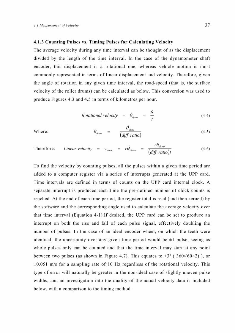
4.1 Measurement of Velocity 37
4.1.3 Counting Pulses vs. Timing Pulses for Calculating Velocity
The average velocity during any time interval can be thought of as the displacement
divided by the length of the time interval. In the case of the dynamometer shaft
encoder, this displacement is a rotational one, whereas vehicle motion is most
commonly represented in terms of linear displacement and velocity. Therefore, given
the angle of rotation in any given time interval, the road-speed (that is, the surface
velocity of the roller drums) can be calculated as below. This conversion was used to
produce Figures 4.3 and 4.5 in terms of kilometres per hour.
t
velocityRotational dynoθθ == & (4-4)
Where: ( )ratiodiffdyno
drum
θθ
&& = (4-5)
Therefore: ( )tratiodiffr
rvvelocityLinear dynodrumdrum
θθ === & (4-6)
To find the velocity by counting pulses, all the pulses within a given time period are
added to a computer register via a series of interrupts generated at the UPP card.
Time intervals are defined in terms of counts on the UPP card internal clock. A
separate interrupt is produced each time the pre-defined number of clock counts is
reached. At the end of each time period, the register total is read (and then zeroed) by
the software and the corresponding angle used to calculate the average velocity over
that time interval (Equation 4-1).If desired, the UPP card can be set to produce an
interrupt on both the rise and fall of each pulse signal, effectively doubling the
number of pulses. In the case of an ideal encoder wheel, on which the teeth were
identical, the uncertainty over any given time period would be ±1 pulse, seeing as
whole pulses only can be counted and that the time interval may start at any point
between two pulses (as shown in Figure 4.7). This equates to ±3º ( 360/(60×2) ), or
±0.051 m/s for a sampling rate of 10 Hz regardless of the rotational velocity. This
type of error will naturally be greater in the non-ideal case of slightly uneven pulse
widths, and an investigation into the quality of the actual velocity data is included
below, with a comparison to the timing method.
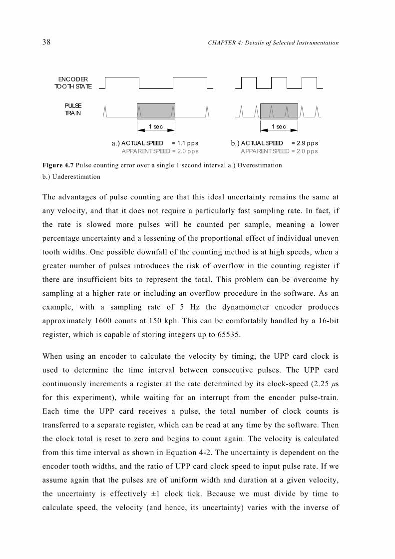
38 CHAPTER 4: Details of Selected Instrumentation
Figure 4.7 Pulse counting error over a single 1 second interval a.) Overestimation
b.) Underestimation
The advantages of pulse counting are that this ideal uncertainty remains the same at
any velocity, and that it does not require a particularly fast sampling rate. In fact, if
the rate is slowed more pulses will be counted per sample, meaning a lower
percentage uncertainty and a lessening of the proportional effect of individual uneven
tooth widths. One possible downfall of the counting method is at high speeds, when a
greater number of pulses introduces the risk of overflow in the counting register if
there are insufficient bits to represent the total. This problem can be overcome by
sampling at a higher rate or including an overflow procedure in the software. As an
example, with a sampling rate of 5 Hz the dynamometer encoder produces
approximately 1600 counts at 150 kph. This can be comfortably handled by a 16-bit
register, which is capable of storing integers up to 65535.
When using an encoder to calculate the velocity by timing, the UPP card clock is
used to determine the time interval between consecutive pulses. The UPP card
continuously increments a register at the rate determined by its clock-speed (2.25 µs
for this experiment), while waiting for an interrupt from the encoder pulse-train.
Each time the UPP card receives a pulse, the total number of clock counts is
transferred to a separate register, which can be read at any time by the software. Then
the clock total is reset to zero and begins to count again. The velocity is calculated
from this time interval as shown in Equation 4-2. The uncertainty is dependent on the
encoder tooth widths, and the ratio of UPP card clock speed to input pulse rate. If we
assume again that the pulses are of uniform width and duration at a given velocity,
the uncertainty is effectively ±1 clock tick. Because we must divide by time to
calculate speed, the velocity (and hence, its uncertainty) varies with the inverse of
ENCODER TOOTH STATE
PULSE TRAIN
1 sec 1 sec
a.) ACTUAL SPEED = 1.1 pps APPARENT SPEED = 2.0 pps
b.) ACTUAL SPEED = 2.9 pps APPARENT SPEED = 2.0 pps

4.1 Measurement of Velocity 39
time. For example, in the ideal-encoder case at say, 10 kph, the UPP card clock will
have time to produce 1637±1 increments between each input pulse (rise only, which
is preferable when timing) from the dynamometer encoder wheel, which is rotating at
28.4 rad/s. At 150 kph, the dynamometer shaft rotates at 426.4 rad/s, resulting in only
109±1 clock counts. Thus at low speed, the velocity error is approximately
±0.002 m/s and at high speeds is almost ±0.4 m/s. To make the best use of this
method, the clock total should be read often and the results averaged, particularly
when the encoder wheel is not entirely uniform. This procedure consumes slightly
more computer processing time than the counting method and also adds an extra
degree of complexity to the software structure. The timing method is most effective
in measuring a pulse frequency that is slow in comparison to the counter clock speed.
The major disadvantages include the loss in precision at high speeds and the
requirement for overflow protection for the counting register at slow speeds, or when
the shaft is stationary.
To compare the practical performance of the counting and timing methods, a series of
constant velocity runs was made under power from the electric motor and with a
dynamometer load present, as for Figures 4.1, 4.3 and 4.5. An analysis of the
resulting random fluctuations (mostly due to the resolution and non-uniformity of the
encoder wheel) is shown in Table 4.2.
Table 4.2 Comparison of uncertainty in velocity calculated by counting, and timing pulses
Note that this data was collected during four separate runs, so the average speeds in
each pair are not identical. As expected, the variation when calculating velocity by
timing pulses was less at the lower speed (≈10 kph) and greater at the higher speed
(≈90 kph). A more consistent figure was achieved by counting, with a range of
approximately 0.05 m/s. In light of a superior performance at high speed, and the
ease with which it could be incorporated into the data acquisition software, the
Calculation method Timing Counting Timing Counting
Average velocity (m/s) 2.758 2.756 24.989 24.967
Maximum measured velocity (m/s) 2.781 2.814 25.081 25.019
Minimum measured velocity (m/s) 2.731 2.711 24.839 24.917
Standard deviation (m/s) 0.0083 0.0167 0.0639 0.0139

40 CHAPTER 4: Details of Selected Instrumentation
counting method was chosen, and has been used for all subsequent velocity data
presented in this thesis.
4.2 Calculation of Acceleration
Once the pulse counting method of calculating velocity had been decided upon, it
was necessary to investigate the most appropriate technique to arrive at the
instantaneous acceleration. Acceleration of the vehicle under test is particularly
useful during driving cycle tests, in which the power absorber may be used to apply
any additional inertial resistance not provided by the flywheels. This additional force
is equal to the difference in equivalent mass between the vehicle and the
dynamometer system, multiplied by the current acceleration.
( ) ( )dtdvmmNforceinertialExtra cdVeq −= (4-7)
Instantaneous acceleration was to be calculated from a discrete series of velocity
measurements, provided by the pulse-counting scheme detailed above. In this section,
a sampling frequency of 10 Hz was used. This is the current sampling rate during
driving cycle tests, although some modes of operation sample at 5 Hz and calculate
acceleration in a similar way.
4.2.1 Instantaneous Gradient
The most obvious way to differentiate the velocity is to use the rate of change over
the last two data points. That is, by computing the difference between two
consecutive speed measurements and dividing by the time interval. This gives an
average value of the acceleration during that time step (i.e. with no lag). However, in
the presence of noise and uncertainty—where the given velocity is not necessarily the
actual, exact velocity—the method is extremely sensitive and returns an acceleration
signal with exaggerated errors, which is not practical for road load calculations. The
resulting acceleration over time is plotted in Figure 4.8 along with a normalised
velocity, so that only departures from the median velocity are shown as non-zero.
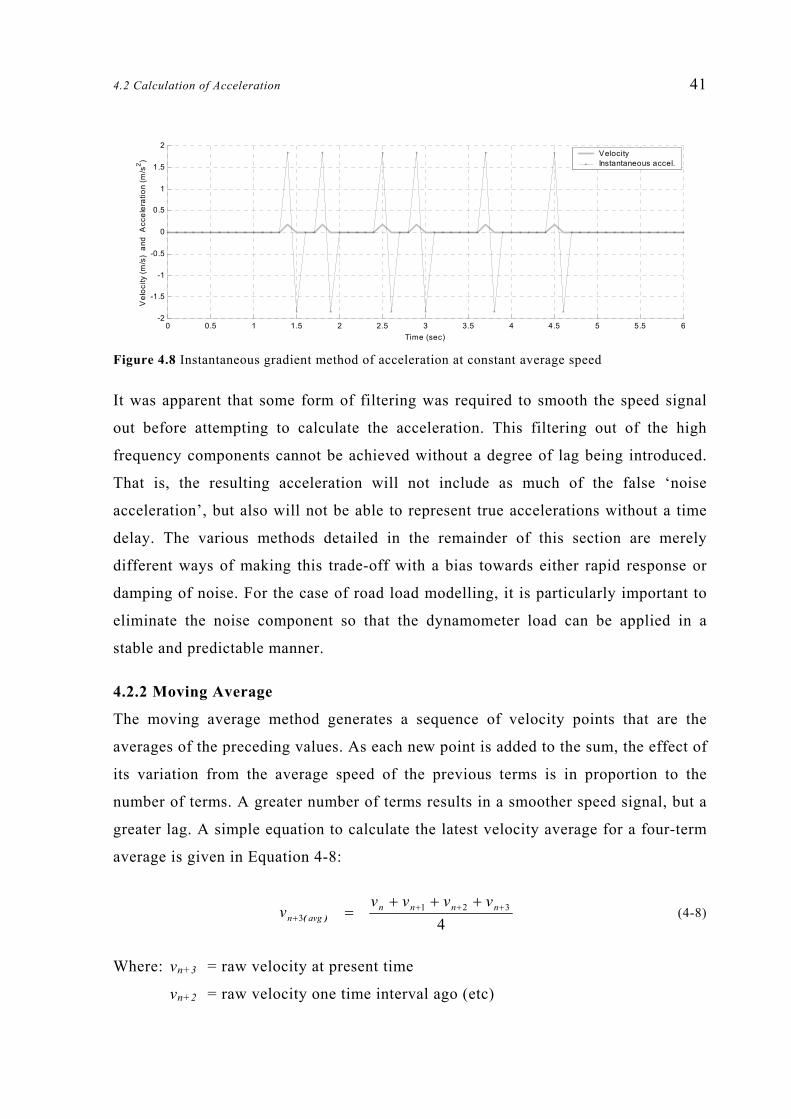
4.2 Calculation of Acceleration 41
0 0.5 1 1.5 2 2.5 3 3.5 4 4.5 5 5.5 6-2
-1.5
-1
-0.5
0
0.5
1
1.5
2
Time (sec)
Vel
ocity
(m/s
) an
d A
ccel
erat
ion
(m/s
2 )Velocity Instantaneous accel.
Figure 4.8 Instantaneous gradient method of acceleration at constant average speed
It was apparent that some form of filtering was required to smooth the speed signal
out before attempting to calculate the acceleration. This filtering out of the high
frequency components cannot be achieved without a degree of lag being introduced.
That is, the resulting acceleration will not include as much of the false ‘noise
acceleration’, but also will not be able to represent true accelerations without a time
delay. The various methods detailed in the remainder of this section are merely
different ways of making this trade-off with a bias towards either rapid response or
damping of noise. For the case of road load modelling, it is particularly important to
eliminate the noise component so that the dynamometer load can be applied in a
stable and predictable manner.
4.2.2 Moving Average
The moving average method generates a sequence of velocity points that are the
averages of the preceding values. As each new point is added to the sum, the effect of
its variation from the average speed of the previous terms is in proportion to the
number of terms. A greater number of terms results in a smoother speed signal, but a
greater lag. A simple equation to calculate the latest velocity average for a four-term
average is given in Equation 4-8:
4
3213
++++
+++= nnnn
avgnvvvv
v )( (4-8)
Where: vn+3 = raw velocity at present time
vn+2 = raw velocity one time interval ago (etc)

42 CHAPTER 4: Details of Selected Instrumentation
Once the latest velocity had been calculated, the previous calculated term can be
subtracted from it and the instantaneous acceleration determined as per Section 4.2.1.
The number of terms is selected on the basis of the required response. A five-term
average was selected by experimentation as having a noise attenuation characteristic
appropriate for this application, and is plotted below in a similar way to Figure 4.8.
Note the delayed negative acceleration that appears when the average returns to zero
after five terms. Plots showing the calculated response to a step acceleration input are
included in Appendix E.
0 0.5 1 1.5 2 2.5 3 3.5 4 4.5 5 5.5 6-0.4
-0.3
-0.2
-0.1
0
0.1
0.2
0.3
0.4
Time (sec)
Vel
ocity
(m/s
) an
d A
ccel
erat
ion
(m/s
2 )
Velocity Moving average accel.
Figure 4.9 Five-term moving average acceleration at constant average speed
4.2.3 Least Squares Differentiator
A sequence of data points can be approximated by fitting a polynomial curve between
them. In this case, a given number of velocity points are approximated by the least
squares method. Once this velocity polynomial has been calculated, the acceleration
is found by analytic differentiation of the curve. The number of data points and the
order of the polynomial may be varied, but in order to provide a unique solution
which will include some smoothing of the velocity, the order of the least squares
polynomial was chosen to be less than the number of data points included. Quadratic
approximation to a four-term series is shown in Appendix F to demonstrate the form
of the least squares solution
The most rapid response to changes in speed was achieved by substituting the end
(latest) time step into the acceleration equation (Equation F-5 in Appendix F).
However, the gradient of the approximated velocity varied steeply when used on
noisy data, particularly with higher-order approximations. By delaying in time by one
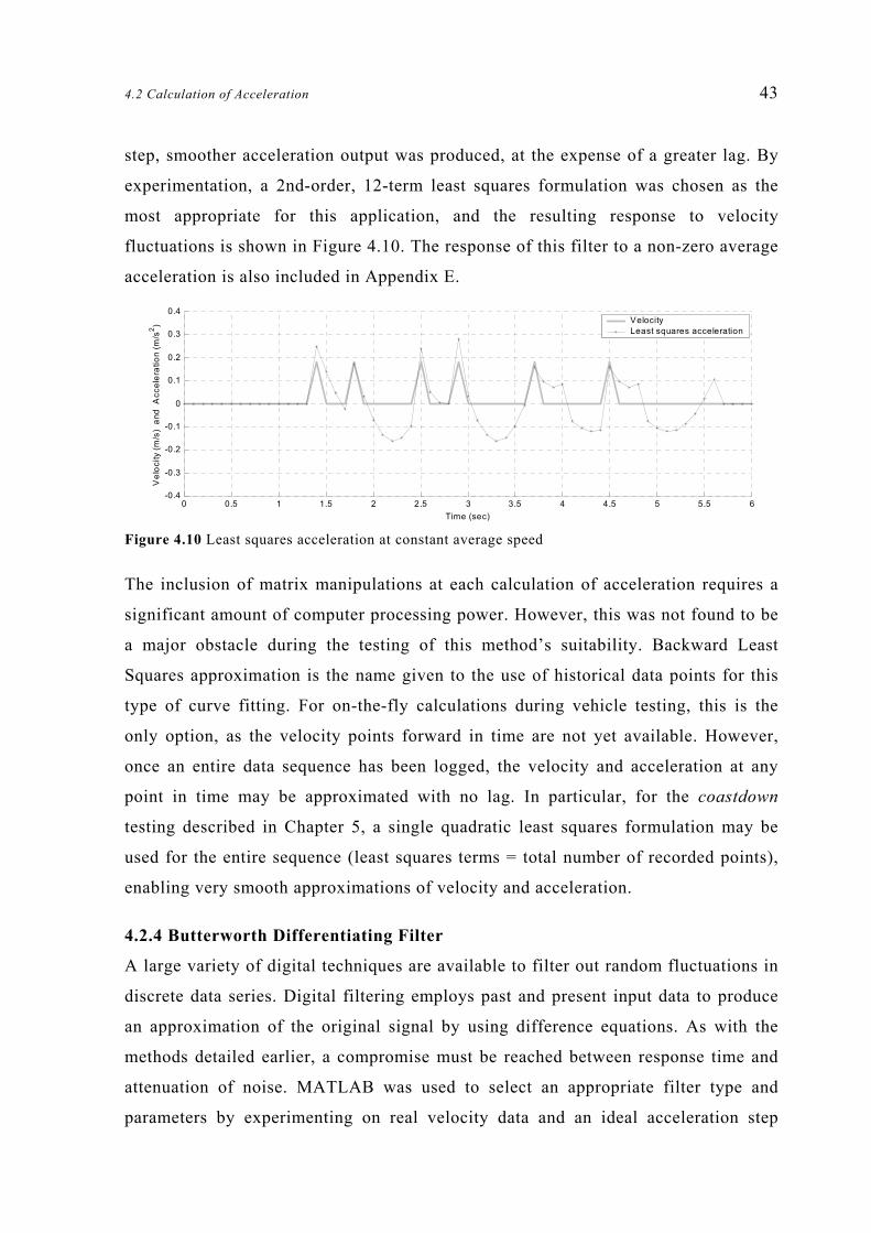
4.2 Calculation of Acceleration 43
step, smoother acceleration output was produced, at the expense of a greater lag. By
experimentation, a 2nd-order, 12-term least squares formulation was chosen as the
most appropriate for this application, and the resulting response to velocity
fluctuations is shown in Figure 4.10. The response of this filter to a non-zero average
acceleration is also included in Appendix E.
0 0.5 1 1.5 2 2.5 3 3.5 4 4.5 5 5.5 6-0.4
-0.3
-0.2
-0.1
0
0.1
0.2
0.3
0.4
Time (sec)
Vel
ocity
(m/s
) an
d A
ccel
erat
ion
(m/s
2 ) Velocity Least squares acceleration
Figure 4.10 Least squares acceleration at constant average speed
The inclusion of matrix manipulations at each calculation of acceleration requires a
significant amount of computer processing power. However, this was not found to be
a major obstacle during the testing of this method’s suitability. Backward Least
Squares approximation is the name given to the use of historical data points for this
type of curve fitting. For on-the-fly calculations during vehicle testing, this is the
only option, as the velocity points forward in time are not yet available. However,
once an entire data sequence has been logged, the velocity and acceleration at any
point in time may be approximated with no lag. In particular, for the coastdown
testing described in Chapter 5, a single quadratic least squares formulation may be
used for the entire sequence (least squares terms = total number of recorded points),
enabling very smooth approximations of velocity and acceleration.
4.2.4 Butterworth Differentiating Filter
A large variety of digital techniques are available to filter out random fluctuations in
discrete data series. Digital filtering employs past and present input data to produce
an approximation of the original signal by using difference equations. As with the
methods detailed earlier, a compromise must be reached between response time and
attenuation of noise. MATLAB was used to select an appropriate filter type and
parameters by experimenting on real velocity data and an ideal acceleration step

44 CHAPTER 4: Details of Selected Instrumentation
input of the type included in Appendix E. A low-pass Butterworth filter was chosen,
which provides an extremely flat passband and acceptable lower order (fewer
historical terms) performance. Filter design was carried out using the MATLAB
butter6 function, which takes the order of the filter and the desired cut-off
frequency as parameters and returns the discrete filter coefficients.
Using the so-called z-domain form, and transforming it to the continuous s-domain, a
differentiation operation can be added to the filter. A full description of the z-
domain, Laplace Transforms, and discrete-continuous filtering can be found in
Franklin et al. [1994]. Multiplication in the s-domain corresponds directly to a
differentiation in the time-domain. So by multiplying the s-domain representation,
then transferring back to the discrete formulation, the digital filter can output filtered
acceleration given a discrete series of velocities. The following equation shows the
filter coefficients calculated in this way, for velocity sampling at 10 Hz.
( ) ( )
0
221122110
bvbvbvavavav nnnnn
n−−−− +−++
=&&
& (4-9)
Where: a0 = 1.024, a1 = 0, a2 = -1.024
b0 = 1, b1 = -1.266, b2 = 0.4706
vn indicates the velocity at the current point
vn-1 indicates the velocity one time interval previous, and so on.
The response of this differentiating filter can be represented on a Bode plot, which is
included in Appendix G and is illustrated on an instantaneous acceleration step in
Figure 4.12. In a discrete sequence, an ‘instantaneous’ increase in acceleration is one
which occurs in the time between two recorded time steps.
6 Courier font denotes software-specific syntax (e.g. entered at MATLAB command prompt)

4.2 Calculation of Acceleration 45
0 0.5 1 1.5 2 2.5 3 3.5 4 4.5 5 5.5 6-0.4
-0.3
-0.2
-0.1
0
0.1
0.2
0.3
0.4
Time (sec)
Vel
ocity
(m/s
) an
d A
ccel
erat
ion
(m/s
2 ) Velocity D ifferentiating filter acceleration
Figure 4.11 Butterworth differentiating filter acceleration at constant average speed
0 0.5 1 1.5 2 2.5 3 3.5 40
0.2
0.4
0.6
0.8
1
1.2
1.4
Time (sec)
Acc
eler
atio
n (m
/s2 )
Ideal acceleration Differentiating filter acceleration
Figure 4.12 Butterworth differentiating filter acceleration response to a step increase in acceleration
It should be noted that the coefficients chosen for a Butterworth filter are frequency
dependent and must be altered if the sampling frequency is to be changed. A separate
filter of the same form was designed by experiment for use with routines operating at
5 Hz.
( ) ( )212 363.0022.1851.0851.0 −−− +−−−= nnnnn vvvvv &&& (4-10)
The response of this formulation to 5 Hz data comparable to the previous acceleration
step is also included in Appendix E.
4.2.5 Filter Selection Summary
The response of the first technique (referred to previously as the Instantaneous
Gradient method) to random fluctuations at constant average velocity immediately
ruled it out, and initiated the search for alternate ways to calculate acceleration. The
Moving Average technique also exhibited unsatisfactory noise attenuation and time
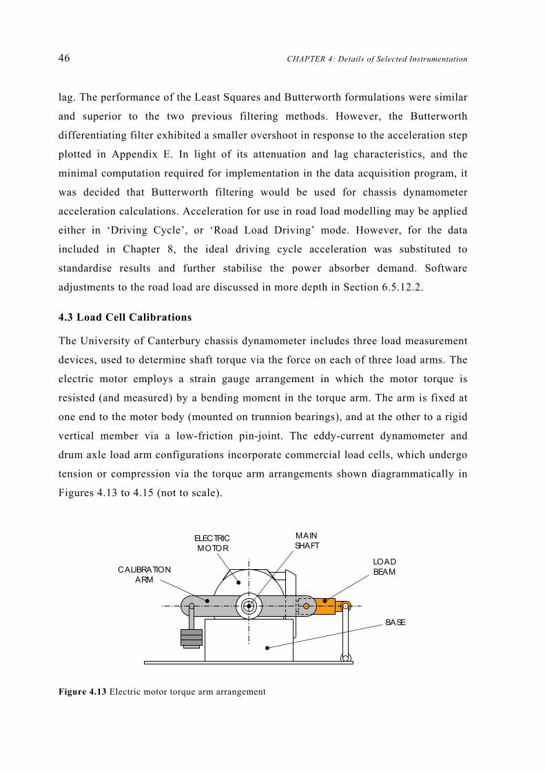
46 CHAPTER 4: Details of Selected Instrumentation
lag. The performance of the Least Squares and Butterworth formulations were similar
and superior to the two previous filtering methods. However, the Butterworth
differentiating filter exhibited a smaller overshoot in response to the acceleration step
plotted in Appendix E. In light of its attenuation and lag characteristics, and the
minimal computation required for implementation in the data acquisition program, it
was decided that Butterworth filtering would be used for chassis dynamometer
acceleration calculations. Acceleration for use in road load modelling may be applied
either in ‘Driving Cycle’, or ‘Road Load Driving’ mode. However, for the data
included in Chapter 8, the ideal driving cycle acceleration was substituted to
standardise results and further stabilise the power absorber demand. Software
adjustments to the road load are discussed in more depth in Section 6.5.12.2.
4.3 Load Cell Calibrations
The University of Canterbury chassis dynamometer includes three load measurement
devices, used to determine shaft torque via the force on each of three load arms. The
electric motor employs a strain gauge arrangement in which the motor torque is
resisted (and measured) by a bending moment in the torque arm. The arm is fixed at
one end to the motor body (mounted on trunnion bearings), and at the other to a rigid
vertical member via a low-friction pin-joint. The eddy-current dynamometer and
drum axle load arm configurations incorporate commercial load cells, which undergo
tension or compression via the torque arm arrangements shown diagrammatically in
Figures 4.13 to 4.15 (not to scale).
Figure 4.13 Electric motor torque arm arrangement
ELECTRIC MOTOR
BASE
CALIBRATION ARM
LOAD BEAM
MAIN SHAFT

4.3 Load Cell Calibrations 47
Figure 4.14 Eddy-current dynamometer torque arm arrangement
Figure 4.15 Drum axle torque arm arrangement (section view, showing load arm, which lies between
the rollers)
The axle assembly, power absorber and electric motor are each supported on trunnion
bearings such that their centre of rotation coincides with the axis of rotation of the
shaft, or—in the case of the axle—the axis of the roller drums. Each load cell force is
opposed by friction in these trunnion bearings, which cannot be measured and
CALIBRATION ARM
DYNAMOMETER MAIN SHAFT
LOAD CELL
BASE
LOAD CELL
ROLLER DRUM
TRUNNION BEARINGS
CALIBRATION ARM ASSEMBLYNOTE: THIS PIN REMOVED
TO APPLY TENSION TO LOAD CELL
DRUM AXLE HALF SHAFT

48 CHAPTER 4: Details of Selected Instrumentation
generates a small error in the load cell reading. The forces at the electric motor, and
dynamometer load cells are shown in Equations 4-11 and 4-12 with notation and
directions as shown in Figure 3.1.
Electric motor load cell reads:
mtmfmemotor FFFF −−= (4-11)
Where: Fmt = electric motor trunnion bearing friction
Dynamometer load cells reads:
dtdfdedyno FFFF −+= (4-12)
The tractive effort BLH U3G1 load cell attempts to measure the tangential force at
the drum surface, which introduces additional complexity to the equation of motion.
Because the roller drums have a significant inertia and frictional effect, the tractive
effort reading delivered by the load cell is not equivalent to the force at the drum
surface, as applied by the vehicle tyres. As well as the load arm reaction force, the
tractive effort input is also opposed by the windage friction on the drum surface and
the inertial mass of the rollers themselves.
TE load cell reads:
( )vmFFFF drdradrtvte &+−−= (4-13)
The tractive effort load cell does not measure the inertial or aerodynamic forces on
the drum assembly, since they do not act on the drum axle housing. These forces may
be measured independently and used to correct the load cell reading (see Section
5.5).
Each of Figures 4.13–4.15 indicate the location of a calibration arm, upon which
known weights were hung in order to calibrate the device. With knowledge of the
mass added and its effective distance from the centre of the shaft, the output of each
device was calibrated by a combination of signal amplification adjustment and
software coefficients. The power absorber and drum axle load cells presented
particular difficulties related to their susceptibility to temperature and the inherent
hysteresis in the mechanical systems.

4.3 Load Cell Calibrations 49
4.3.1 Temperature Effect
After an initial calibration of the dynamometer load cell, it was discovered that the
results—particularly the readings when no load was applied—were not consistent. An
investigation was made into the effects of ambient temperature on the zero reading of
the dynamometer load cell. Regular readings of temperature were taken using a
thermocouple-type digital thermometer while slowly heating the air in the chassis
dynamometer laboratory. At each temperature reading, a small load was applied to
each side of the load arm in turn to remove possible hysteresis. Also, a load cell
measurement was made with 68 kg (equating to approximately 340 Nm) on the
weigher arm in a positive direction (i.e. compression of the load cell, as explained in
Section 3.2). The results of this trial are shown in Figure 4.16 below with air
temperature on the x-axis and zero-load reading on the y-axis.
16 17 18 19 20 21 22 23 24 25-1
-0.5
0
0.5
1
Air temperature ( C)
Torq
ue re
adin
g at
zer
o lo
ad (N
m)
O Figure 4.16 Temperature effect on eddy-current dynamometer zero reading
It can be seen that there was a significant decrease in the zero readings with an
increase in air temperature. This offset was also noted in the 68 kg measurements, as
the torque measured on the load cell tended to decrease with an increase in
temperature. Figure 4.17 below shows the difference between the average zero
readings as shown above, and the 68 kg readings recorded during the same
temperature run. It is interesting to note that the difference does not appear to follow
the same trend as the zero readings.
This indicates that the temperature effect manifests itself as a pure offset as opposed
to a change in the span of the device, which would give an increasingly greater error
z

50 CHAPTER 4: Details of Selected Instrumentation
16 17 18 19 20 21 22 23 24 25
339.5
339.6
339.7
339.8
339.9
340
340.1
340.2
340.3
340.4
340.5
Air temperature ( C)
Load
cel
l rea
ding
less
zer
o re
adin
g (N
m)
O
Figure 4.17 Temperature effect on the eddy-current dynamometer reading with 68kg on the load arm
magnitude with greater temperature. It should be noted that the load cell devices used
do include some form of temperature compensation to allow for the changes that
result when the electronics heat up. However, it would appear that this compensation
circuitry on both the dynamometer and the drum axle load cells may be damaged or
have aged and can no longer provide a predictable output. Replacement of these
faulty load cells is suggested. However, to obtain useful results with the existing
equipment, some form of software compensation was desired. Measuring the air
temperature and adjusting the torque readings accordingly may have been possible,
but without a knowledge of the exact relationship between the temperature of the
ambient air and the state of the internal load cell electronics, such a technique would
be difficult to put into practice. Instead, it was decided that the load cell should be
manually zeroed (by removing hysteresis and taking a zero reading) at the beginning
of each testing session. The constant flow of air from the external cooling fans in the
laboratory should ensure a constant temperature during testing. The A/D voltage
during this zeroing process is stored by the computer for future tests. A constant
calibration span is maintained, but an offset is added so that zero torque is recorded
whenever this offset voltage is encountered. The software routine to handle this
zeroing is further described in Section 6.5.6.
4.3.2 Tractive Effort Hysteresis
The load cell arrangements on the electric motor, eddy-current dynamometer and the
drum axle all exhibited some degree of hysteresis. That is, the friction of the load
arm arrangement, and/or the electronic characteristics of the load cells caused the

4.3 Load Cell Calibrations 51
load reading to have a ‘memory’ of sorts. For example, after a high loading,
hysteresis in the load cell system resulted in an error in the direction of this load,
even after the load was removed. However, in the case of the motor and
dynamometer, a small load applied on each side of the load arm in turn was sufficient
to remove this error during calibration. The drum axle load cell, which measures the
tractive effort applied by a vehicle under test, was found to generate greater errors
due to a change in load direction.
Hysteresis in the tractive effort load cell was most likely due to a combination of the
greater complexity in the load arm mechanism (meaning greater friction) and the age
of the load cell. The problem was compounded by the large torque loads experienced
by this shaft. The magnitudes of loading and the arrangement of the load arm meant
that maximal calibration loads in the positive direction (load cell in compression,
using the calibration linkage shown in Figure 4.15) tended to lift the axle off its
bearings, obviously affecting the loading angles and load cell readings. One way to
overcome this lifting was to clamp the axle (at the drum surface) thus preventing
vertical motion while allowing freedom of rotation. However, the increased
compressive force on the static axle bearings contributed further towards hysteresis.
By rotating the system at a constant speed during calibration, a large proportion of
this static friction hysteresis could be eliminated. The electric motor was used to turn
the drum shaft over slowly, while a vehicle was placed on the rollers to serve a
clamping role. This rotation introduced its own set of errors related to the frictional
resistance to motion and any misalignment of the vehicle on the drums. In particular,
whenever the drums are rotated by the electric motor, a finite torque must be applied
to the axle to overcome the bearing friction. This torque, which is applied at the
differential, is measured by the tractive effort load cell, which effectively records the
forces between the drum shaft and the main shaft. To overcome this difficulty, the
zero load cell reading was first taken in the absence of any motion or the clamping
load. Then the vehicle was placed on the rollers, the motor was started, and the
calibration arm engaged. The offset at this point was balanced by the addition of
masses in a trial and error fashion onto the calibration arm, to return the tractive
effort reading to its previous zeroed value. The calibration masses were then added in
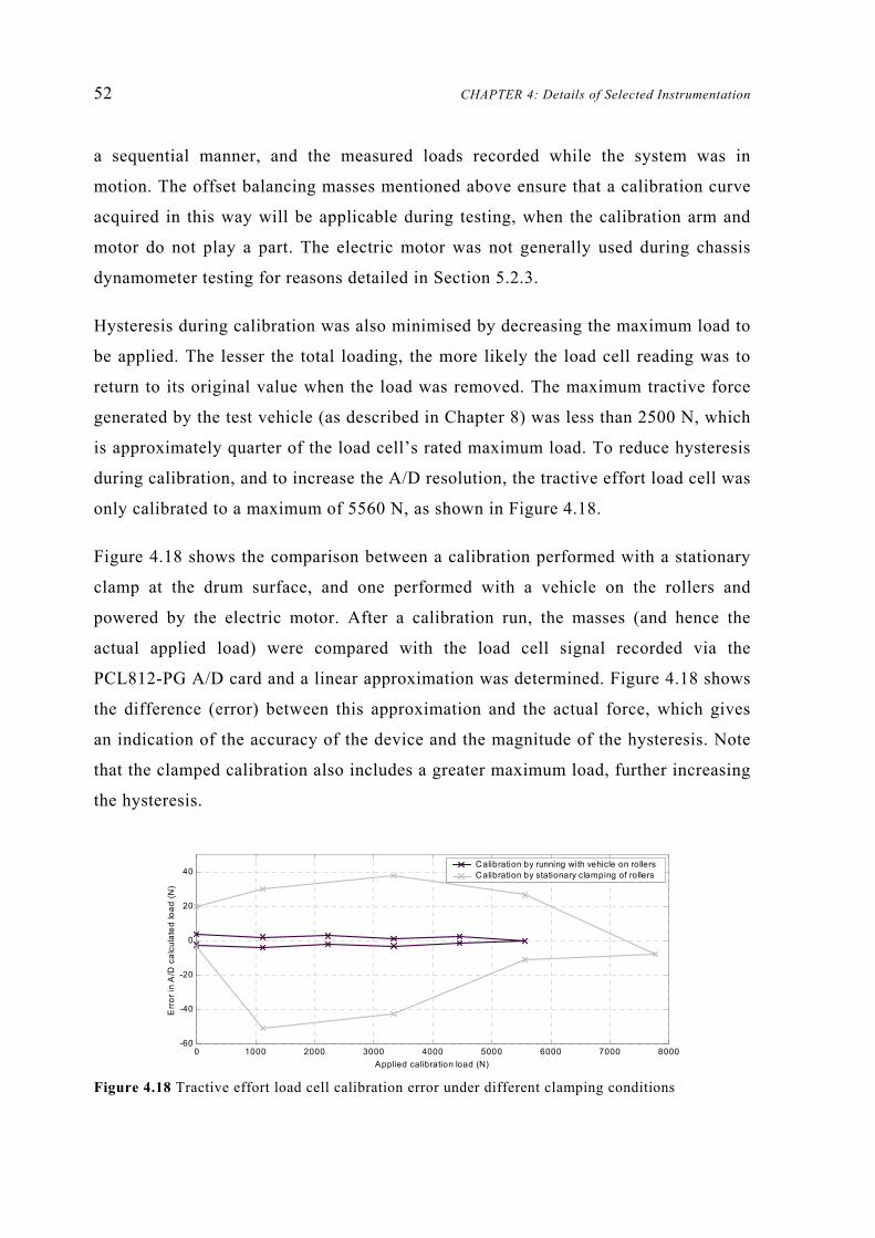
52 CHAPTER 4: Details of Selected Instrumentation
a sequential manner, and the measured loads recorded while the system was in
motion. The offset balancing masses mentioned above ensure that a calibration curve
acquired in this way will be applicable during testing, when the calibration arm and
motor do not play a part. The electric motor was not generally used during chassis
dynamometer testing for reasons detailed in Section 5.2.3.
Hysteresis during calibration was also minimised by decreasing the maximum load to
be applied. The lesser the total loading, the more likely the load cell reading was to
return to its original value when the load was removed. The maximum tractive force
generated by the test vehicle (as described in Chapter 8) was less than 2500 N, which
is approximately quarter of the load cell’s rated maximum load. To reduce hysteresis
during calibration, and to increase the A/D resolution, the tractive effort load cell was
only calibrated to a maximum of 5560 N, as shown in Figure 4.18.
Figure 4.18 shows the comparison between a calibration performed with a stationary
clamp at the drum surface, and one performed with a vehicle on the rollers and
powered by the electric motor. After a calibration run, the masses (and hence the
actual applied load) were compared with the load cell signal recorded via the
PCL812-PG A/D card and a linear approximation was determined. Figure 4.18 shows
the difference (error) between this approximation and the actual force, which gives
an indication of the accuracy of the device and the magnitude of the hysteresis. Note
that the clamped calibration also includes a greater maximum load, further increasing
the hysteresis.
0 1000 2000 3000 4000 5000 6000 7000 8000-60
-40
-20
0
20
40
Applied calibration load (N)
Err
or in
A/D
cal
cula
ted
load
(N)
Calibration by running with vehicle on rollers Calibration by stationary clamping of rollers
Figure 4.18 Tractive effort load cell calibration error under different clamping conditions

4.3 Load Cell Calibrations 53
Note that Figure 4.18 contains only positive loading for each calibration technique. It
was found that the load cell outputs of the dynamometer torque and tractive effort
transducers were dependent on the direction of loading. That is, the voltage for a
given load cell tension was different to the voltage output under a compressive load
of the same magnitude. For this reason, both the eddy-current dynamometer and
tractive effort load cell calibrations have separate calibration curves for each
rotational direction. Refer to Appendix C for full details of these load cell calibration
functions and equations.
Results from the rolling calibration runs lead to an estimated measurement
uncertainty of ±9 N. Additional uncertainty was introduced by the temperature
effects discussed in Section 4.3.1, and the requirement for correction of the tractive
effort load cell reading for the inertia and windage friction of the roller drum
assembly (see Section 5.5.3). The overall tractive effort uncertainty was expected to
be ±50 N during moderate changes in velocity (e.g. driving cycle testing) and ±10 N
under constant speed conditions (e.g. vehicle mapping tests).

CHAPTER 5:
Inertia and Friction Determination
5.1 Inertia Overview
Testing on the chassis dynamometer involves the application of a known force at the
surface of the vehicle tyres. This force is represented by Equation 3-8, where Fde and
Fme are the inputs from the power absorber (Froude eddy-current dynamometer) and
motor (ASEA D.C. motor) respectively. A free-body diagram of all the forces acting
on the chassis dynamometer is shown in Figure 3.1.
With knowledge of the materials and components as well as the relevant shaft sizes, a
calculation of the equivalent mass of each component could be made, as was carried
out by Raine [1981]. However, experimental confirmation of this calculation was
sought, and is detailed in Sections 5.2 and 5.3.
The combined equivalent mass of the motor, dynamometer, drums, and shafts was
determined by experimentation (see Section 5.3). Calculation of the flywheel inertias
based on their thickness and diameter was thought to be sufficiently accurate, as no
major simplifications were needed. Similarly, the combined frictional coefficients
were found by experiment, and require ongoing recalibration to account for wear-
related changes in friction. The individual mass and frictional characteristics of the
drum axle assembly were also determined in order to generate useful tractive effort
measurements from the roller drum load cell.
It should be noted that the particular method used to find these inertial and frictional
constants determined which of these were to be included in subsequent testing
procedures. For example, for calibrations under power from the electric motor, the
friction, Fmf and the actual motoring force Fme are measured as a single torque at the
motor load cell (see Equation 4-11). The motor controller adjusts to give a certain
output torque, meaning that the internal friction—whatever it may be—is motored

56 CHAPTER 5: Inertia and Friction Determination
out, rendering the friction and motoring forces indistinguishable, unless independent
measurements were available. If the chassis dynamometer were subsequently run
without a motoring force from the electric motor, only the unknown friction would
act on the shaft, leaving an undefined variable in the motion equations. In a similar
way, the dynamometer load cell only detects the combined forces Fdf and Fde at the
power absorber. Sections 5.2 and 5.3 include several different calibration techniques
and their associated difficulties. The interrelationship between friction and inertia
forces, as well as the specific forces which are not included (e.g. those that are
motored out) are explained in detail below.
As suggested by Equation 3-8, inertial forces (mcd dv/dt) are only encountered during
changes in velocity of the dynamometer shaft. Therefore, any experimentation to
determine the inertia of a physical system must involve either acceleration or
deceleration. The most common method of calibrating for inertia is by coastdown of
the system. In the case of a chassis dynamometer, the system is brought up to a
certain speed (either by external means, or a motor if one is present) then allowed to
decelerate under the influence of friction while measurements of time and velocity
are made. In some cases, a known power-absorber and/or motoring torque is also
applied to generate different rates of deceleration. The presence of motoring or
power-absorbing forces means that the system cannot strictly be thought of as
‘coasting’ down. However, for the purposes of this discussion any deceleration under
constant dynamometer or motor load will be referred to as a coastdown. For inertia
calibration, the dynamics of the University of Canterbury chassis dynamometer are
similar to those of Figure 3.1, but without the complication of a vehicle on the
rollers. This means that the tractive force at the roller drum surface (FV) is zero, with
the exception of windage friction on the rollers, which can be included in the overall
friction force.
fricdynomotorcd FFFdtdvm −−= (5-1)
Where: Ffric = combined chassis dynamometer friction forces (excluding
contribution from motor and dynamometer)

5.2 Inertia Determination Using the Motor 57
Note: dtdv is negative during deceleration
It can be seen from this equation that the determination of inertia using the
coastdown technique demands recording of the motoring/power-absorbing forces as
well as a prior knowledge of the frictional characteristics of the system as a whole.
These frictional forces can be determined in a separate experiment or accounted for
by setting up parallel tests in which all friction terms can be mathematically
cancelled.
5.2 Inertia Determination Using the Motor
To calculate the system inertia, two different techniques were attempted involving
power input from the electric motor. The first is a common method wherein the
frictional characteristics of the system are determined in a separate calibration, then
used to calculate the inertia during a coastdown run. The second method eliminates
the need to determine the friction by running an acceleration and a deceleration run
in which the friction forces can be cancelled during calculation. These motor-driven
methods were subject to the limitations of the chassis dynamometer configuration,
and this difficulty is discussed in Section 5.2.3.
5.2.1 Calculating Friction from Constant Speed Trials
By assuming that the friction of the various system components is dependent only
upon the rotational velocity, the frictional coefficients can be determined in a series
of constant velocity tests. Under constant speed and with a known (possibly zero)
dynamometer torque Equation 5-1 may be reduced to:
fricdynomotor FFF += (5-2)
Where: 2210 vfvffF dddfric ++= (5-3)
In the case of the University of Canterbury chassis dynamometer, the load cells
indicate either the internal friction of the motoring/absorbing devices (if no control
demand is made) or the total force applied by them. Thus, the total friction sought in
Equation 5-2 does not include any power-absorber or electric motor friction

58 CHAPTER 5: Inertia and Friction Determination
component. In order to achieve a stable force from the dynamometer, constant load
demands were implemented in torque mode on the power absorber. Constant speed
was maintained by the ASEA motor controller at several predefined set-points, and
the torque (converted to force) at each load cell was recorded, along with the speed.
Thus the total friction force at each velocity could be calculated. A minimum of three
speed points was required to solve for f0d, f1d, f2d, simultaneously, but a greater
number were generally recorded and the resulting data used to calculate a quadratic
equation for Ffric as a function of velocity on a least squares basis. General use of the
least squares velocity-time approximation is included in Appendix F, and this
technique may be extended to other data sets such as the friction-velocity
relationship. An example of several constant velocity friction data sets is included in
Appendix H with the accompanying calculated friction coefficients. To obtain a
single final value, the total frictions from each run were combined to arrive at an
average least squares approximation, from which the average coefficients were taken
(see also Appendix H). Over the range of motor and dynamometer torques available,
there appeared to be a large variation at each velocity of ±20 N in the total friction
recorded. In addition, negative constant and squared term coefficients (f0, f2) were
calculated for the runs employing 100 Nm power absorber torque. Since this would
lead to the impossible case of a negative total friction force at low speeds, doubt was
cast on the suitability of using the motor and power absorber in this way to determine
the system friction.
Using the average system friction coefficients as calculated above (f0d = 13.28,
f1d = 6.86, f2d = -0.031) the equivalent mass of the chassis dynamometer could be
found by carrying out a coastdown and applying Equation 5-1. By measuring each of
the other components—including acceleration differentiated from a least squares
approximation of the velocity signal—the equivalent mass could be found at each
instant during the deceleration. Coastdown data such as velocity and dynamometer
torque were recorded at 0.1 second intervals using a purpose-designed C++ program.
To minimise experimental error, a series of tests were performed at different
dynamometer loads and the resulting inertias were averaged during each coastdown.
An idealised sample of a single inertia calculation is illustrated in Figure 5.1, while
the complete coastdown results are tabulated in Appendix I.

5.2 Inertia Determination Using the Motor 59
Time
v
t
Fmotor = 100 N
Fdyno = 400 N
Ffric = 50 N
v = 20 m/s
2m/s50.−=dtdv
Figure 5.1 Example of inertia coastdown
From Equation 5-1:
kg700=−
−−=
−−=
5.050400100
dtdv
FFFm fricdm
cd
The average mcd was found to be 716.6 kg, with experimental variations of ±14 kg
(std. dev. = 9.2%) assuming the friction forces during each run were as calculated
earlier. That is, the inertia of a vehicle with an equivalent mass of 716.6 kg could be
simulated by the chassis dynamometer with no additional motoring or power-
absorbing torque.
During the friction calibrations, constant speed trials conducted at higher
dynamometer torques tended to yield a lower total friction (see Appendix H). That is,
the apparent difference between the motor and power absorber torques (Equation 5-2)
was less at any given velocity, when it should have remained the same if the
equipment was performing as expected. Therefore, during coastdowns with high
power absorber loads (e.g. 100 Nm), the averaged friction from Appendix H may be
higher than the apparent friction calculated at that particular dynamometer torque.
When this average friction is applied to Equation 5-1, the resulting inertia is lower
for the runs employing high power absorber torque, and higher for those with less
power absorber load (see Appendix I). Since the averaging of these frictional
constants provided a somewhat arbitrary result, another method was sought to
calculate the equivalent mass of the system.
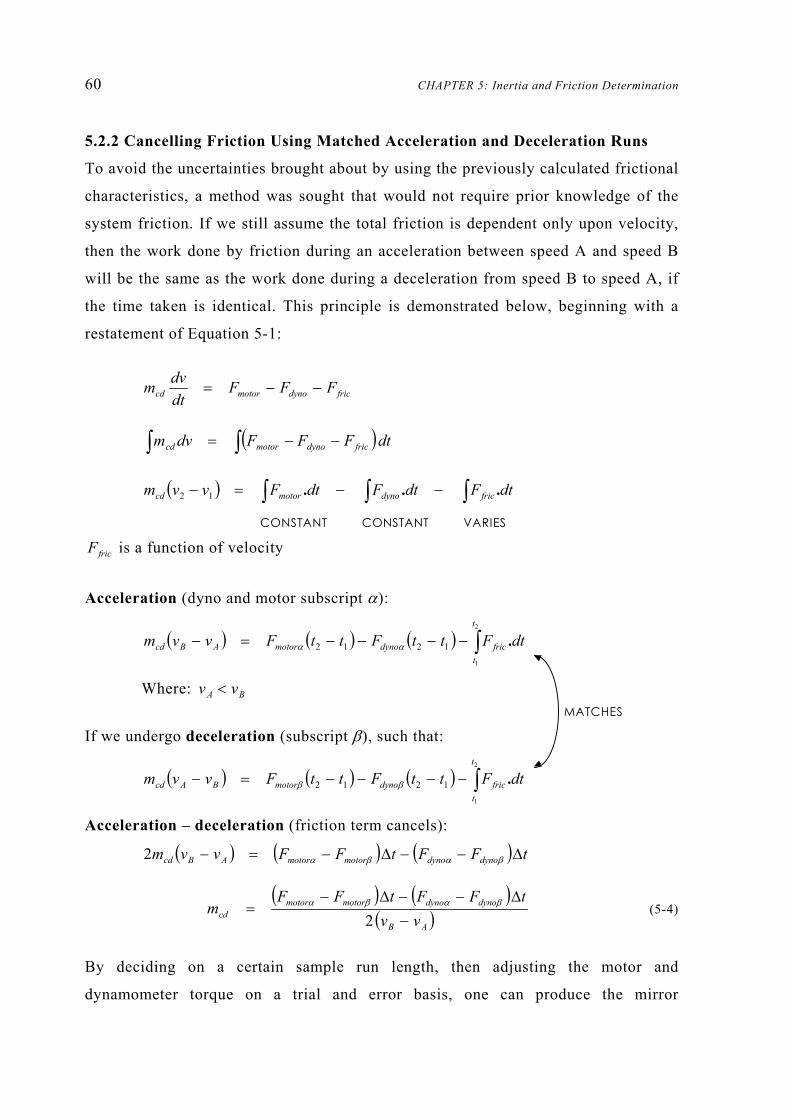
60 CHAPTER 5: Inertia and Friction Determination
5.2.2 Cancelling Friction Using Matched Acceleration and Deceleration Runs
To avoid the uncertainties brought about by using the previously calculated frictional
characteristics, a method was sought that would not require prior knowledge of the
system friction. If we still assume the total friction is dependent only upon velocity,
then the work done by friction during an acceleration between speed A and speed B
will be the same as the work done during a deceleration from speed B to speed A, if
the time taken is identical. This principle is demonstrated below, beginning with a
restatement of Equation 5-1:
fricdynomotorcd FFFdtdvm −−=
( )∫∫ −−= dtFFFdvm fricdynomotorcd
( ) ∫∫∫ −−=− dtFdtFdtFvvm fricdynomotorcd ...12
CONSTANT CONSTANT VARIES
fricF is a function of velocity
Acceleration (dyno and motor subscript α):
( ) ( ) ( ) ∫−−−−=−2
1
1212
t
tfricdynomotorABcd dtFttFttFvvm .αα
Where: BA vv <
If we undergo deceleration (subscript β), such that:
( ) ( ) ( ) ∫−−−−=−2
1
1212
t
tfricdynomotorBAcd dtFttFttFvvm .ββ
Acceleration – deceleration (friction term cancels):
( ) ( ) ( ) tFFtFFvvm dynodynomotormotorABcd ∆−−∆−=− βαβα2
( ) ( )
( )AB
dynodynomotormotorcd vv
tFFtFFm
−∆−−∆−
=2
βαβα (5-4)
By deciding on a certain sample run length, then adjusting the motor and
dynamometer torque on a trial and error basis, one can produce the mirror
MATCHES

5.2 Inertia Determination Using the Motor 61
acceleration for any prior deceleration (assuming the maximum motor power is
sufficient). Thus, with all the elements of Equation 5-4 known, the equivalent mass
of the chassis dynamometer could be calculated. This approach was implemented in a
series of acceleration and deceleration pairs to determine the repeatability for a given
time span and speed interval, and the variation between runs of differing speeds or
acceleration/deceleration rates. The motor torque was varied manually on the
instrument panel or by entering a fixed D/A demand, and all data was again captured
by a C++ program, which read the A/D values and UPP card velocity at each
0.1 second interval. Several sets of acceleration/deceleration runs are included in
Appendix J, and the averaged results for each set are shown in Table 5.1 below.
Table 5.1 Summary of acceleration/deceleration inertia determination trials
Within each set of data shown in Table 5.1 (and included in Appendix J) the velocity
differences, and the average motor and dynamometer force readings, each typically
varied by less than 0.5%. However, the range of masses calculated in this way was
approximately 32 kg, which was similar (in terms of variation) to the results obtained
from the previous method using coastdowns with assumed friction values. The
calculated equivalent mass of the chassis dynamometer (without flywheels) was
noticeably lower (709.4 vs. 716.6 kg).
Results Set Velocity Velocity F motor F dyno Massv A (m/s) v B (m/s) (N) (N) ∆ t (s) m cd (kg)
Deceleration 16.68 22.16 257.66 517.02 9.90
Acceleration 16.63 22.16 723.83 208.17 9.90 696.2
Deceleration 12.65 20.76 278.82 719.39 9.90
Acceleration 12.68 20.77 901.81 210.90 9.90 691.2
Deceleration 19.54 24.94 165.41 405.97 9.90
Acceleration 19.49 24.90 948.18 398.67 9.90 723.1
Deceleration 14.40 19.43 151.46 381.89 9.90
Acceleration 14.39 19.47 898.56 396.25 9.90 717.5
Deceleration 9.08 13.86 144.31 373.88 9.90
Acceleration 9.10 13.86 864.88 401.79 9.90 719.0
Average 709.4
E
A
B
C
D
62 CHAPTER 5: Inertia and Friction Determination
5.2.3 Limitations of the Electric Motor
As mentioned in Chapter 2, the ideal chassis dynamometer operation involves both a
power absorber and a motoring capacity, both of which can be rapidly set depending
on the load and inertia simulation requirements. For example, in the case where a
vehicle’s inertia is greater than that of the dynamometer flywheels, a motoring torque
is required during deceleration, and a resisting torque is required during acceleration
(see Equation 4-7).
During the inertia calibrations in Sections 5.2.1 and 5.2.2 in which the eddy-current
dynamometer was operating at high load, the electric motor torque reading became
more noisy, and also increased in magnitude slightly. Investigation revealed that the
most likely cause was that the high-current, high-frequency eddy-current demand was
coupling with the low-current motor load-cell (and hence, control feedback) signal.
In addition, the response time of the motor and dynamometer to their respective
command signals was a factor. Particularly in the case of the electric motor, it was
necessary to set the load demand several seconds before the initial coastdown speed
point was reached, in order that the system should have time to settle down. Rapid
application of large loads resulted in torsional vibrations, which also lasted a few
seconds, but these were not as significant as the electric motor settling period. This
lag in motor output torque was especially evident at low speeds, or when starting the
system from stationary.
One possible solution to the difficulty of slow motor response is to apply a constant
motoring torque, which is balanced by a varying power absorber torque as required.
Equation 3-10 contains a term Fnet, which determines the net effect of the motor and
power absorber (Fdyno – Fmotor). The constant motor torque must be at least equal to
the greatest negative Fnet that will be encountered. When lesser motoring loads are
required, the dynamometer—with its superior response characteristics—is
programmed to overcome the unwanted proportion (or the entirety) of the motor
torque. In the course of most driving cycle testing, the vehicle is required to stop for
length of time, which also creates problems for the chassis dynamometer. The power
absorber requires a rotational movement within its electric field to create a force, and
thus it cannot produce any motion-resisting torque at zero velocity. In addition, the

5.2 Inertia Determination Using the Motor 63
electric motor is at its least stable at zero velocity, and so applying the vehicle brakes
is not a full solution. The instability of the electric motor is demonstrated in Figure
5.2, which shows the response to a step command while the system is held stationary
under braking. While step commands would not be required under a constant
motoring-load scheme, the experiment shows that the motor controller was generally
susceptible to disturbances while stationary.
0 5 10 15 20 25
0
5
10
15
20
25
30
35
Time (sec)
Torq
ue (N
m)
Demand torque Achieved motor torque
Figure 5.2 Response of electric motor controller at zero velocity
Oscillations with a period of approximately 1 second can be seen, which take a
significant amount of time to dissipate. An attempt to improve performance was
made by implementing a software controller in series with the existing analogue
hardware. With additional control, it was also expected that the demand following
characteristics could also be improved. Note that while the relationships between
D/A demand voltage and output torque were largely linear (see Appendix C for
calibration) small non-linear inaccuracies were observed.
Proportional-Integral gain, and simple Integral-only controllers were tested, but were
found to further exacerbate the present oscillations due to the feedback lag. That is,
the time delay between the software acquiring the latest motor torque, and the
sending of another constant torque demand to the analogue controller—which also
exhibits a finite delay. The results for an Integrator controller at zero velocity are
included in Appendix K.
In light of this unsatisfactory response, it was decided that the electric motor would
be used only for warming the system up, or bringing the rollers up to speed for
64 CHAPTER 5: Inertia and Friction Determination
coastdown testing and the like. With the motoring force reduced to zero, Fnet in
Equations 3-10 and 3-11 becomes equal to the power absorber force, Fdyno. It is
evident that under some road load conditions, the required force, Fnet will become
negative. This can be the case if the relative frictional coefficients of the
dynamometer system are larger than those of the vehicle, or more significantly, under
changes in velocity. For example, the inertial component (mVeq – mcd)dv/dt will
become negative during acceleration if the equivalent mass of the vehicle being
modelled is exceeded by the chassis dynamometer mass. In such cases a
dynamometer motoring capability is desired. Where none is available, errors arise as
the motion of the vehicle is resisted to a greater degree than it would be under the
same conditions on the road. However, making use of the flywheel set, (mVeq – mcd)
should never exceed 60 kg, which was thought to be acceptable in light of the
apparent inaccuracies brought about by the use of the electric motor. Also, in testing
situations where the energy absorbed by the vehicle during braking is not important,
the dynamometer equivalent mass may be set lower, so that less braking will be
needed during deceleration, with the shortfall in rotational inertia being
supplemented with an additional positive power absorber load for acceleration
phases.
Excluding the motoring force creates an additional problem in that the previous
methods used to calculate the inertia and friction do not include the frictional
characteristics of the motor when it is not applying a load. The friction of the
unemployed motor was previously included in the Fmotor value and is not easily
separated, as described in Section 5.1. The chassis dynamometer as a whole should
be used for testing in the same mode of operation as it was calibrated. Thus, a method
of finding the system inertia and friction was desired that would not require direct
use of the electric motor.
5.3 Inertia Determination Without the Motor
By default, the only dynamometer situation with no vehicle present and no input from
the motor is a coastdown (or no motion at all), be it under torque from the power
absorber, or friction only. Equation 5-5 below is a restatement of the coastdown

5.3 Inertia Determination Without the Motor 65
Equation 5-1, without the presence of a motoring force, and with the friction terms
(including the unpowered electric motor friction) grouped together as a single value.
−−=
dtdv
FFm fricdyno
cd (5-5)
Measuring Fdyno, and calculating dv/dt, we have two unknowns at each instant: the
equivalent mass, mcd, which remains constant throughout, and Ffric which is assumed
to be dependent upon instantaneous velocity. Therefore, if we have recorded data
from two coastdowns under different dynamometer loads—and hence, rates of
deceleration—the total friction term can be cancelled at any one velocity, leaving
only one unknown value. For example, if two generic coastdowns are performed
under FdynoA and FdynoB, the velocity vs. time relationships take the form shown in
Figure 5.3.
1 1 .5 2 2 .5 3 3 .5 4 4 .5 5 5 .5 6
1
1 .5
2
2 .5
3
3 .5
4
4 .5
5
Coastdown A
Time
Vel
ocity
v'
1 1 .5 2 2 .5 3 3 .5 4 4 .5 5 5 .5 6
1
1 .5
2
2 .5
3
3 .5
4
4 .5
5
Coastdown B
Time
Vel
ocity
v'
dynoAfricAA
cd FFdtvdm −−=
′
dynoBfricBB
cd FFdtvdm −−=
′
Figure 5.3 General form of two different coastdowns under dynamometer torque
At the desired speed point ( v ′ ) marked on the diagram, the friction terms FfricA and
FfricB are identical, so by subtracting the second coastdown equation from the first,
we arrive at Equation 5-6.
( ) dynoBdynoABAcd FFvvm −−=− && (5-6)
Where: dtdvv =&

66 CHAPTER 5: Inertia and Friction Determination
From which the equivalent mass, mcd can be calculated. It should be noted that mcd is
constant for any choice of velocity, so that the two coastdowns can be matched in any
number of ways, provided dv/dt and Fdyno are also measured. Figure 5.4 shows
various combinations of the same coastdown pair.
1 1 .5 2 2 .5 3 3 .5 4 4 .5 5 5 .5 6
1
1 .5
2
2 .5
3
3 .5
4
4 .5
5
Time
Vel
ocity
α v
1 1 .5 2 2 .5 3 3 .5 4 4 .5 5 5 .5 6
1
1 .5
2
2 .5
3
3 .5
4
4 .5
5
Time
Vel
ocity
β v
1 1 .5 2 2 .5 3 3 .5 4 4 .5 5 5 .5 6
1
1 .5
2
2 .5
3
3 .5
4
4 .5
5
Time
Vel
ocity
γ v
Figure 5.4 Two coastdowns combined at several different velocities
In practice, the electric motor was used to bring the system up to approximately
20 kph above the maximum recorded velocity (to ensure a stable state before the
desired speed range was reached). At this point, the motor was switched off, so that
no residual or random current could be introduced during the coastdown. A known
dynamometer load was then applied via a D/A signal from the computer, and the
velocity and torque were recorded from when the upper speed was reached until the
minimum recorded velocity was registered. Eddy-current dynamometer control and
data acquisition were accomplished in a simple purpose-written C++ program, while
the analysis of coastdown data and simultaneous solving for the inertia were carried
out in a MATLAB function (see program solve_inertia on CD). It was found
that the dynamometer equivalent masses calculated according to Equation 5-6
exhibited a small speed-dependent variation. For this reason, it was decided that
several coastdown runs should be carried out at several different dynamometer
torques, and the results averaged. This variation in inertia with the velocity at which
it was calculated is shown in Figure 5.5, where a set of three coastdown runs have
been combined in each of the three possible ways. That is, if data exists for
coastdowns under nominal loads of 60 Nm, 80 Nm, and 100 Nm respectively, the
simultaneous solution may be calculated at any velocity by combining the 60 Nm and
80 Nm, the 60 Nm and 100 Nm, or the 80 Nm and 100 Nm data sets.

5.3 Inertia Determination Without the Motor 67
30 40 50 60 70 80 90 100 110
664
666
668
670
672
674
676
678
680
682
684
Velocity (kph)
Cal
cula
ted
equi
vale
nt m
ass
(kg)
60Nm and 80Nm runs combined 60Nm and 100Nm runs combined80Nm and 100Nm runs combined
Figure 5.5 Variation in calculated equivalent mass with differing velocity and dynamometer loads
The variation over this range of speeds and loads (similar to those encountered
during vehicle testing) was found to be of the order of 2% in this case. To obtain a
single dynamometer inertia value, the calculations were averaged over the whole
speed range during post-processing, and the coastdown data at each power-absorber
torque was itself the average of eight individual runs under such conditions.
Satisfactory repeatability was observed with these averaged sets of data. A series of
32 individual coastdowns with nominal dynamometer torques of 40, 60, 80, and 100
Nm identified the base inertia (no additional flywheels) as 673.8 kg. Averaging the
eight files at each power-absorber torque, and combining these torque sets in
different ways produced equivalent masses with a standard deviation of 2.3 kg
(0.3%). Full results of these repeatability tests are included in Appendix L.
Determination of the system inertia by coasting down without torque from the
electric motor was identified as the most appropriate method in light of the
difficulties with the motor control and the repeatability of the various techniques
employed in Section 5.2.
5.3.1 Base Inertia Correction
Further coastdown tests were conducted in a similar way with the addition of
flywheels to increase the total equivalent mass. In terms of repeatability, the results
obtained in these trials were comparable to those detailed in Section 5.3 and
Appendix L. The mass added by the inclusion of these flywheels was relatively easy
to calculate since each is a simple steel disc. The flywheel set was originally
constructed with this in mind, to give round numbers for the equivalent mass. A

68 CHAPTER 5: Inertia and Friction Determination
description of the chassis dynamometer flywheel set is included in Section 2.2. The
moment of inertia (in kg.m2) of each flywheel is equal to the moment of inertia of a
solid disc of the same size, less the removed portion that the shaft passes through.
2
4trIdiscρπ
= (5-7)
Where: ρ = material density (kg/m3)
r = disc radius (m)
t = disc thickness (m)
Moments of inertia at the fast (flywheel) end of the shaft can be converted into
equivalent mass at the roller drums by first converting to moment of inertia at the
slow (drum) end:
( ) slowslow IratiodiffI = (5-8)
Note: diff ratio = 43/7
Then calculating the equivalent mass at the drum surface:
2drrIm = (5-9)
Where: rdr = drum radius = 0.6 m
If these equivalent masses are known, the only unknown inertia is that of the system
with no flywheels attached, as was previously calculated. However, tests involving
some or all of these flywheels revealed that the coastdown method did not exactly
predict the equivalent mass steps that had been calculated using Equations 5-7 to 5-9.
Table 5.2 shows the experimental equivalent mass of several flywheel combinations
against the nominal values calculated from their size. The inertia of the flywheels
alone is represented by subtracting the equivalent mass of 674 kg calculated in
Section 5.3. Figure 5.6 shows the error between the experimental and the nominal
flywheel mass values.
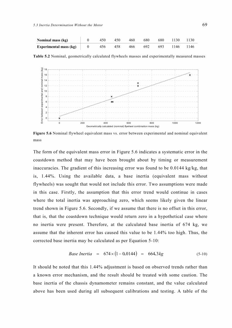
5.3 Inertia Determination Without the Motor 69
Table 5.2 Nominal, geometrically calculated flywheels masses and experimentally measured masses
0 200 400 600 800 1000 1200
0
2
4
6
8
10
12
14
16
18
Geometrically calculated (nominal) flywheel combination mass (kg)
Err
or b
etw
een
expe
rimen
tal a
nd n
omin
al m
ass
(kg)
Figure 5.6 Nominal flywheel equivalent mass vs. error between experimental and nominal equivalent
mass
The form of the equivalent mass error in Figure 5.6 indicates a systematic error in the
coastdown method that may have been brought about by timing or measurement
inaccuracies. The gradient of this increasing error was found to be 0.0144 kg/kg, that
is, 1.44%. Using the available data, a base inertia (equivalent mass without
flywheels) was sought that would not include this error. Two assumptions were made
in this case. Firstly, the assumption that this error trend would continue in cases
where the total inertia was approaching zero, which seems likely given the linear
trend shown in Figure 5.6. Secondly, if we assume that there is no offset in this error,
that is, that the coastdown technique would return zero in a hypothetical case where
no inertia were present. Therefore, at the calculated base inertia of 674 kg, we
assume that the inherent error has caused this value to be 1.44% too high. Thus, the
corrected base inertia may be calculated as per Equation 5-10:
( ) kgInertiaBase 3664014401674 .. =−×= (5-10)
It should be noted that this 1.44% adjustment is based on observed trends rather than
a known error mechanism, and the result should be treated with some caution. The
base inertia of the chassis dynamometer remains constant, and the value calculated
above has been used during all subsequent calibrations and testing. A table of the
Nominal mass (kg) 0 450 450 460 680 680 1130 1130
Experimental mass (kg) 0 456 458 466 692 693 1146 1146

70 CHAPTER 5: Inertia and Friction Determination
total equivalent masses resulting from the various flywheel combinations that can be
acheived on the dynamometer is included in Appendix A.
5.4 Friction Determination from Coastdown Data
Having arrived at an appropriate equivalent mass, and assuming that the motoring
force is zero, Equation 5-5 now has only one unknown quantity at any given velocity
and acceleration; that of the system friction, Ffric. The chassis dynamometer is subject
to frictional forces from the bearings, differential losses, and air resistance on the
flywheels and drum. Each of these forces acts in a direction opposite to the direction
of motion, and may vary according to the rotational velocity. It was assumed for
simplicity that the combination of frictional forces would be represented as a single
quadratic equation depending only upon speed, as represented in Equation 5-3. Thus,
whereas Equation 5-5 was solved simultaneously using two sampled coastdowns
(Equation 5-6), the three frictional coefficients require solving of data from three or
more points, which can be from the same coastdown. Note that the term coastdown
here indicates a deceleration under torque from the eddy-current dynamometer, as
mentioned in Section 5.1.
With a knowledge of velocities and dynamometer loads over the course of a
coastdown run, Equation 5-5 can be rearranged to solve for the total frictional force
at a given speed. Equivalent mass (constant) and Fdyno are known at each point, while
the friction is dependent upon velocity.
dynocdfric FdtdvmF −= (5-11)
Data was collected in the same way as the inertia calculations of Section 5.3 with
several coastdown runs being performed at each of four different dynamometer loads.
As a repeatability trial, the total friction was calculated at shaft speeds equivalent to
35 kph and 105 kph at the roller drums for 32 separate coastdowns under various
dynamometer torques. At 35 kph the average frictional force was 73.4 N (referenced
to the drum surface) with a standard deviation of 1.5 N (2.0%). At 105 kph the
average friction was found to be 136.5 N with a standard deviation of 1.1 N (0.8%).
These variations were in the range of uncertainty of the load cell readings, and

5.4 Friction Determination from Coastdown Data 71
therefore the method was deemed sufficiently repeatable. A complete table of results
is included in Appendix M. It should be noted that frictional coefficients calculated
in a similar way to the equivalent inertias of Section 5.3 may be subject to the same
systematic error in magnitude mentioned in Section 5.3.1. However, a 1.4% error in
the total friction would also be less than the smallest measurable torque, and thus any
such error was ignored.
For each coastdown, the velocity series was approximated by a least squares
quadratic equation, as detailed in Appendix F. From this equation, the approximate
acceleration (dv/dt in Equation 5-11) at any point can be calculated by
differentiation. In order to solve for each of the frictional coefficients (f0d, f1d, f2d) the
total friction was calculated from Equation 5-11 at each of three speeds (e.g. 35, 70
and 105 kph) and averaged over the various dynamometer load runs. This provided
three known friction totals at three known velocities:
2210 AdAddfricA vfvffF ++= (5-12a)
2210 BdBddfricB vfvffF ++= (5-12b)
2210 CdCddfricC vfvffF ++= (5-12c)
These three equations could then be solved simultaneously to arrive at unique values
of f0d, f1d, and f2d. For example, the data summarised in Appendix M was collected
during coastdowns with flywheels adding to an equivalent mass of 1114kg, and
yielded friction coefficients thus:
20060473040 vvFfric ... −+= (5-13)
Where v = velocity in m/s
The friction mechanisms at work in this situation dictate that each of these
coefficients should be greater then zero. However, a small negative value was
calculated for the velocity-squared term, which may have been result of experimental
errors. The magnitude of this term also justifies the use of a three-term
approximation for friction, as opposed to higher orders. That is, no significant

72 CHAPTER 5: Inertia and Friction Determination
increase in accuracy would be expected if the relationship between friction and
velocity were modelled as a cubic, for example.
It was evident that the frictional characteristics of the system change depending on
the number of flywheels rotating with the shaft (introducing air resistance) and the
number that are stationary on the shaft (friction between the moving inner and
stationary outer race of each bearing). Also, the friction may vary throughout the life
of the chassis dynamometer as various components age and wear. Thus, it was
necessary to include the friction calibration procedure in the main dynamometer
program. Details of this implementation are included in Section 6.5.5. Given the
repeatability of the calculated frictional forces shown in Appendix M, it was thought
that the averaging of three or four coastdowns (under different torques) would
provide satisfactory friction coefficients. It is recommended that the coefficients for
each flywheel combination be recalculated at least every two months during use and
that the dynamometer be thoroughly warmed up before any testing session. Warming
up of the system generally entails running under power from the electric motor or a
test vehicle to ensure all the rotating components have reached a state of thermal and
frictional stability. Details of the warm up routine can be found in Section 6.5.8.
5.5 Tractive Effort Load Cell Correction
As mentioned in Chapter 4, the characteristics of the roller drum assembly need to be
known before useful measurements can be made using the tractive effort load cell.
Equation 4-13 shows that the output force from a vehicle on the rollers is balanced by
the inertial forces of the drums, the aerodynamic frictional forces on the rollers, and
the other combined resistances from the flywheels and power absorber that are
measured by the load cell. In order to record the actual force at the surface of the
vehicle tyres, the equivalent mass and frictional characteristics of the roller drums
must be known, along with the instantaneous velocity and acceleration.
5.5.1 Roller Drum Inertia
Calculation of the drum assembly inertia was performed in almost exactly the same
way as for the total system inertia, except that the measurement of torque at the eddy-
current dynamometer was replaced by the roller drum load cell reading. The tractive

5.5 Tractive Effort Load Cell Correction 73
ROLLER SURFACE
TRUNNION BEARINGS
LOAD CELL
Fte
Fdra
Fdrt
v, v .
effort load cell is set up to read the tangential force as at the surface of the drums by
means of the load arm and computer calibration coefficients. A simplified free-body
diagram represents the relationship between the trunnion-mounted axle assembly and
the fixed support (measured by the load cell).
Figure 5.7 Free body diagram of forces on the drum axle assembly during coastdown
Where: v = velocity at drum surface (m/s)
v& = acceleration at drum surface (m/s2, negative during coastdown)
teF = reaction force measured at load cell (N)
drtF = drum axle trunnion bearing friction (N)
draF = aerodynamic friction on drum surface (N)
During a coastdown, each of these forces opposes the direction of motion, and the
acceleration, v& is negative. Referencing the forces to the drum surface, gives an
equation of motion as shown in Equation 5-14.
dradrttedr FFFvm −−−=& (5-14)
Fdrt represents the Coulomb friction at the trunnion bearings, which introduces
hysteresis when the direction of loading is changed. Because the direction of this

74 CHAPTER 5: Inertia and Friction Determination
force is related to the tractive force direction (not the direction of motion), it cannot
be included in velocity-dependent friction equations, and must be neglected. This
omission introduces an error, which is not particularly significant in the
determination of the drum inertia since the direction of the tractive force does not
change in the course of a coastdown run.
Since Fte is known, and v& can be calculated at any point during a coastdown, the
drum friction, Fdra can be cancelled between two different runs to allow a solution for
mdr as per Equation 5-6. Again, averaging over several different dynamometer loads
(which varies Fte and the rate of deceleration) a single value for the equivalent mass
was arrived at. Recording data from a total of 32 separate coastdowns with four
different dynamometer loads, the average equivalent mass (as at drum surface) was
found to be 599.3 kg with a standard deviation of 3.6 kg (0.6%). In the absence of
accurate empirical calculations (like those used in Section 5.3.1), it was decided not
to subtract the 1.4% error that was present in the whole system calibration, since the
error may have been due to the dynamometer load cell, which was not used during
the drum assembly calculations. Appendix N contains a full table of sampled results
leading to the calculation of the roller drums’ equivalent mass. Raine [1981] lists
geometrically calculated inertias for each element of the dynamometer system. In
these calculations, the roller drums and axle assembly account for 89.8% of the total
system inertia, with no flywheels present. The equivalent mass of 599 kg shown
above represents 90.3% of the 664 kg base inertia. This provides a measure of
vindication for both the experimental and geometric calculation approaches.
5.5.2 Roller Drum Friction
Once the inertia of the roller drum assembly had been determined, a similar method
to that detailed in Section 5.4 could be used to find the windage friction force, Fdra.
As in the case of the whole system, the resistance to motion was modelled as having
a second-order relationship to the rotational velocity. However, the aerodynamic
friction on the drum surfaces is present only while the drums are rotating, and thus
f0dr = 0. A series of coastdowns was again used to determine the repeatability of the
method. At 35 kph the total friction force was found to be 4.6 N with a standard
deviation of 1.6 N (35%), while the total friction at 105 kph was 22.6 N with a

5.5 Tractive Effort Load Cell Correction 75
standard deviation of 1.7 N (8%). A complete set of drum friction results is included
in Appendix O. The level of repeatability (in absolute terms) was comparable to the
calculations of friction for the chassis dynamometer as a whole (see Section 5.4),
although the percentage error was significantly greater in the case of the drum
friction. Provision is also made in the main computer program for the regular
updating of these frictional coefficients. Whenever new friction coefficients are
generated for the system as a whole, the option is given for the user to also record the
tractive effort data to calculate the roller drum friction as well. Again, a description
of this routine is included in Chapter 6.
5.5.3 Effectiveness of the Load Cell Correction
In order to determine the actual force applied by a vehicle to the rollers, the
equivalent mass of the drum assembly and its frictional coefficients are determined
beforehand using the methods above. During operation, the instantaneous velocity
and acceleration, and the load cell force are continuously changing with time. It was
necessary to determine whether the response of these updated parameters was
sufficient to accommodate the rapid changes that occur during driving cycle testing.
While an instantaneous response would be ideal, it was realised that some delay
would be inevitable due to the requirement for acceleration filtering (introducing a
time lag) as detailed in Section 4.2. The load cell signal also includes a degree of
damping, and it was important that the measured tractive effort and the calculated
velocity and acceleration were all appropriate when solving Equation 4-13 for FV at
each point in time. A series of experiments were carried out recording the
acceleration, raw load cell signal, velocity-dependent friction and the final, corrected
tractive effort. By accelerating and decelerating the chassis dynamometer under
power from the electric motor and power absorber respectively, there is no tractive
force (as from a vehicle) on the rollers. Therefore, the corrected tractive force should
remain zero through any increase or decrease in velocity. The constituents
represented in Figure 5.8 are shown in Equation 5-15:
drfricdrumloadcellcorr FdtdvmFF ++= (5-15)
CORRECTED
TRACTIVE EFFORT
CORRECTION COMPONENT
RAW TRACTIVE
EFFORT
=
+

76 CHAPTER 5: Inertia and Friction Determination
0 5 10 15 20 25 30 35 40 45-2000
-1500
-1000
-500
0
500
1000
1500
Time (sec)
Trac
tive
Effo
rt an
d C
orre
ctio
n F
orce
(N)
Net corrected tractive effort Inertia and friction correctionRaw load cell tractive effort
1 2 3 4 7 6 5 8
Figure 5.8 Tractive effort correction response under motor and dynamometer power
Table 5.3 Tractive effort correction response test phases (see Figure 5.8)
It can be seen in Figure 5.8 that the average corrected tractive effort remains at zero,
as it should when no force is applied at the roller surface. However, there are several
small excursions from this zero point at the changes in acceleration. This indicates
that the time lag in the acceleration calculation exceeds any lag in the load cell
signal. For example, under a rapid increase in speed (e.g. at the beginning of
Phase 2), the correction component does not immediately include the energy that is
being expended in accelerating the drums, and therefore the corrected tractive effort
momentarily reads too low. This method of correcting the tractive effort load cell
signal was applied throughout the testing described in Chapter 8, often making use of
an approximated or ‘ideal’ acceleration (see Section 6.5.12.2).
Phase Activity
1 Zero load from motor and dyno. Speed = 0 m/s
2 Motor brings system up to speed. Maximum acceleration = 2.2 m/s2
3 Constant speed control from motor. Speed = 14.5 m/s
4 Dyno load 50 Nm added. Small deceleration.
5 Motor restores constant speed. Dyno load = 50 Nm. Speed = 14.5 m/s
6 Motor load removed. Dyno load = 50 Nm. Average deceleration = 0.6 m/s2
7 Dyno load increased to 150 Nm. Average deceleration = 1.2 m/s2
8 System comes to rest. Speed = 0 m/s

CHAPTER 6:
Control and Data Acquisition Software
This chapter contains both a general description of the chassis dynamometer software
program and specific details of its functionality and implementation in the C++
programming language. Significant decisions regarding the overall form and data
sharing with other applications are highlighted, as well as the constraints that have
lead to some of these decisions. Each mode of operation requires a different on-
screen appearance and data-handling capabilities, and these are discussed in Sections
6.5.4–6.5.12. Computer program files are shown in upper case, while the names of
specific software functions and syntax are printed in courier font.
6.1 Program Layout
The chassis dynamometer control software consists of an executable program written
and compiled using Borland C++ version 3.1. The layout and menu options may be
viewed by running this executable, which is included—along with each of the source
code files—on the CD accompanying this thesis. However, without the necessary
A/D electronics and file structure, several warnings are triggered and most of the
functionality is disabled. Upon running, the user is greeted by the screen display
shown in Figure 6.1. The majority of the coloured screen displays included in this
section are printed in black and white, with arrowed notes included for the readers’
benefit. The colour of the background, and indeed all colours throughout the program
can be adjusted by setting numerical constants in the C++ source files.
The Turbo Vision set of object-oriented classes and libraries allows a Windows-like
interface wherein the user can navigate using a mouse or key strokes through a series
of pull-down menus and display windows. Selections are made with the usual
‘buttons’, which can be activated by the mouse button, or the Space or Enter keys.
x

78 CHAPTER 6: Control and Data Acquisition Software
Figure 6.1 Initial display screen showing available pull-down menus
Standard Turbo Vision menu and window classes were used to produce screen
displays like those shown in Figure 6.2.
Within this structure, the various testing and calibration functions can be accessed,
each having their own set of user preferences, which are stored in separate text files.
These preference files are saved at each edit so that the latest settings are still usable
if the program is shut down and restarted. Appendix P lists every available menu
option in the main program. It should be noted that some operations—such as the
‘Flywheel Setup’ function—are required before every test and as such can be
accessed from more than one place in the program.
The principal function of the program is to facilitate chassis dynamometer testing.
During a test, data must be sent to the computer, received, and saved, while also
providing user feedback to the monitor. A program loop is used that performs each of
these operations, then waits for a timed interrupt before repeating the process. This
allows the program to record and send data at regular intervals in time and is further
discussed in Section 6.5.3.
PULL-DOWN MENUS
“ HOT-KEY” FUNCTIONS
PRESENT TIME AVAILABLE HEAP MEMORY

6.2 Programming Constraints 79
Figure 6.2 Example of a window showing the available user options
6.2 Programming Constraints
Early on in the project, it was decided that the final control program should be a DOS
application, using the Turbo Vision classes and libraries to achieve a graphical user
interface. There were several reasons that this format was chosen over a Windows-
based application, including the programming work already carried out, and
difficulties with program running speed and interrupt timing under Windows.
In 1994 a former student, Neil Glasson, had written a C++ program to control the
operations of the University of Canterbury’s engine dynamometer. The overall
concept and form of this software was similar to what would be required for the
chassis dynamometer, and a small number of routines could be renamed and used in
their existing form. Although crossover from the engine dynamometer program was
minimal in the long run, the layout and programming style provided a useful
springboard for the writing of the chassis dynamometer software. In addition, Neil
Glasson had written software for the visual driving cycle display. This scrolling
graphic was implemented in the final program with minor additions, and is detailed
in Section 6.5.12.1.
SELECTION BUTTONS
NUMERICAL ENTRY BOXES ACCEPT / CANCEL
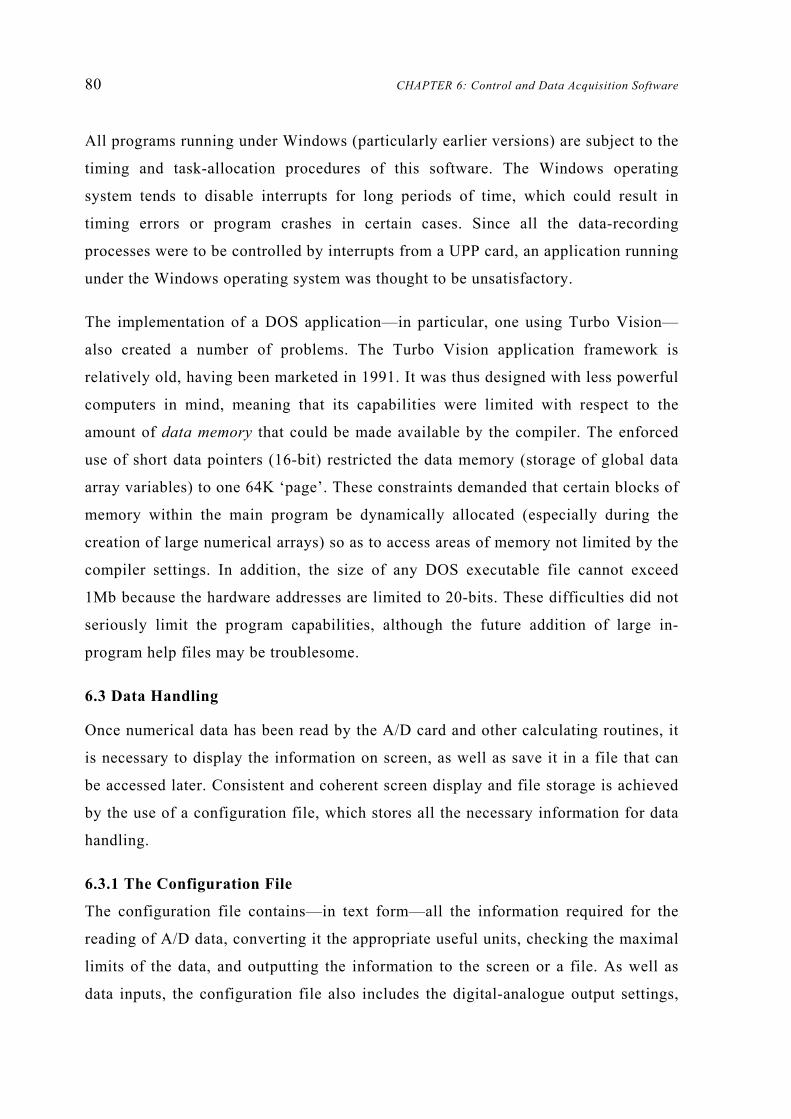
80 CHAPTER 6: Control and Data Acquisition Software
All programs running under Windows (particularly earlier versions) are subject to the
timing and task-allocation procedures of this software. The Windows operating
system tends to disable interrupts for long periods of time, which could result in
timing errors or program crashes in certain cases. Since all the data-recording
processes were to be controlled by interrupts from a UPP card, an application running
under the Windows operating system was thought to be unsatisfactory.
The implementation of a DOS application—in particular, one using Turbo Vision—
also created a number of problems. The Turbo Vision application framework is
relatively old, having been marketed in 1991. It was thus designed with less powerful
computers in mind, meaning that its capabilities were limited with respect to the
amount of data memory that could be made available by the compiler. The enforced
use of short data pointers (16-bit) restricted the data memory (storage of global data
array variables) to one 64K ‘page’. These constraints demanded that certain blocks of
memory within the main program be dynamically allocated (especially during the
creation of large numerical arrays) so as to access areas of memory not limited by the
compiler settings. In addition, the size of any DOS executable file cannot exceed
1Mb because the hardware addresses are limited to 20-bits. These difficulties did not
seriously limit the program capabilities, although the future addition of large in-
program help files may be troublesome.
6.3 Data Handling
Once numerical data has been read by the A/D card and other calculating routines, it
is necessary to display the information on screen, as well as save it in a file that can
be accessed later. Consistent and coherent screen display and file storage is achieved
by the use of a configuration file, which stores all the necessary information for data
handling.
6.3.1 The Configuration File
The configuration file contains—in text form—all the information required for the
reading of A/D data, converting it the appropriate useful units, checking the maximal
limits of the data, and outputting the information to the screen or a file. As well as
data inputs, the configuration file also includes the digital-analogue output settings,

6.3 Data Handling 81
such as multiplication factors and upper and lower limits. By storing all these details
in a single file, standardised settings can be used by different testing routines, and
changes to the C++ code will not affect the specifics of A/D or D/A operations.
Prior to any operation involving the PCL-812PG card, the configuration file is
opened and the important information stored in arrays that can be accessed during
data collection operations. This routine can be found in the source code in file
CH_CMDS.CPP, routine read_AtoD_config. The parameters in the
configuration text file (given a file extension *.cfg) may be edited by the user from
within the control program, or using any text editor, such as MS Notepad7. A printout
of a sample configuration file is included in Appendix Q, with a description of the
each parameter.
6.3.2 File Input/Output
All testing routines (as well as the calibration operations) involve the saving of
captured data in a file for later use either by the control program, or to be viewed by
the user. Before any of the testing routines begin saving data, a header is written in
the user-defined save-file which includes time and date information, as well as the
type of test, the last measured frictional coefficients of the system, and the details of
all the data to be collected (e.g. ‘Roller Speed (kph)’). Typically, during each of the
timed loops mentioned in Section 6.1, all the required data is read from the PCL-
812PG and PCLD-889 cards according to the settings in the configuration file, and
temporarily stored in one or more numerical arrays. At the end of each loop, a single
file-writing operation transfers this array data to the file in a prescribed order and
form.
The form of the save-file was intended to be comprehensible as text only, while also
maintaining portability for other applications like MATLAB and Excel. In particular,
delimiting commas have been included to aid its opening in Excel, and the post-
processing MATLAB programs discussed in Chapter 7 include routines that transfer
the file data into matrices from which the information can be edited or plotted. An
7 Copyright Microsoft Corporation

82 CHAPTER 6: Control and Data Acquisition Software
example of a saved data file is included in Appendix R with a description of each of
the text components. Example data files can also be found on the CD accompanying
this thesis, in the directory Sample Output Files.
6.4 Mathematics Functions
Solving sets of simultaneous equations using a computer program is most easily
achieved with matrix algebra. The methods discussed in this section are included as
part of the chassis dynamometer control software for the calculation of least squares
approximations, and the simultaneous solving from coastdown data to determine the
system friction (Section 4.4).
The elementary array structures of C++ do not immediately lend themselves to
calculations involving matrices of more than one dimension. This is due to the
sequential storage and recall of data in numerical arrays. To work with two-
dimensional arrays, it was necessary to set up a structure for each matrix that
included row and column data to access the sequential block of memory in which the
numbers were stored.
For example, a 3×4 matrix would be stored with the following information: Number
of rows = 3, number of columns = 4, as well as pointer to the memory location of the
first element. Element (2,3) for example, could then be accessed in a fictional 3×4
matrix as shown in Figure 6.3.
Figure 6.3 Example of matrix storage and indexing
Matrix Data:
C++ Memory Storage: (name = array, rows = 3, cols = 4) INDEX
Element (2,3) accessed by C++ command: array[cols×(2-1) + 3 - 1]
= array[6]
DATA
9 10 11 12
1 2 3 4
8 7 6 5
0 1 2 3 4 5 6 7 8 9 10 11 12
9 10 11 12 1 2 3 4 8 7 6 5

6.5 Control Program Functionality 83
Having allocated the memory and defined the row width and column height of each
matrix, separate routines were generated to complete various simple matrix
manipulations. Matrix transposition, inversion (using the Gauss-Jordan method) and
multiplication and are included in MATH.CPP. Least squares coefficients are
calculated using the following equation as shown in Appendix F.
( ) yXXX TT 1−=α (6-1)
Solving for frictional coefficients also requires multiplying and inverting matrices as
shown below:
At each speed point: ( ) frictiontotalFfff
vv fric ==
2
1
021
Combining data from three points:
=
c
b
a
cc
bb
aa
FFF
fff
vvvvvv
2
1
0
2
2
2
111
FX =f
And solving for coefficients: ( ) FX 1−=f (6-2)
6.5 Control Program Functionality
This section details each of the most important tasks carried out by the chassis
dynamometer control software. Where possible, the sequence of events has been
represented in the form of a flow diagram, while C++ programming specifics and
syntax has been minimised. However, the names of several classes and functions
have been included so that reference can be made to the source code (supplied on
CD) if desired.
6.5.1 Turbo Vision idle Function
Most Turbo Vision applications include the same background operations that keep
the program running and wait for what are known as events. An event is essentially a
piece of information that requires an action. For example, keyboard inputs, mouse
button presses, and messages sent from one part of the program to another are all

84 CHAPTER 6: Control and Data Acquisition Software
events. The chassis dynamometer control program includes a loop that continuously
retrieves any new events (Turbo Vision’s getEvent) and acts on these events
(handleEvent). The getEvent function checks for keyboard and mouse inputs,
then calls the idle function. These operations can be simplified in flow diagram
form (Figure 6.4).
Figure 6.4 Flow diagram of continuous background loop of main program
Within the idle function, there are several commands that update the state of the
program. For example, the on-screen clock is checked against the computer clock and
updated, the heap-memory indicator displays the latest size of available memory, and
the digital inputs (e.g. equipment off/on and mode switches) are read via the PCL-
812PG card. Most importantly, this idle function—so called because it is executed
when only when there are no other tasks awaiting action—creates an event which
instructs the program to run the function designated by cmUpdate. Each mode of
dynamometer operation has its own implementation of the cmUpdate function,
which usually involves all the other ongoing tasks such as reading the A/D signals,
sending out D/A demands, and writing data to a file. The generic form of this
updating routine is discussed in Section 6.5.3.
Exit Program ?
Check Keyboard and Mouse Events
idle
Act on the Event
NO
YES
Start Program

6.5 Control Program Functionality 85
6.5.2 Setting Test Parameters
Each task performed on the chassis dynamometer has various parameters that alter
the mode of operation, or the nature of the results. Instead of entering new values for
these parameters each time a certain function is carried out, the details are stored in a
series of files which are read by the program before commencing a particular
operation. These user-defined settings include: vehicle details such as mass and
frictional coefficients, the current flywheel combination, which A/D configuration
file to use, and the test duration. If any particular option is not changed by the user
before running the dynamometer, the most recently entered value is read from the
appropriate file.
In most cases, the necessary parameters are chosen by selecting button-type options,
or through a keyboard input such as typing in the desired numerical value. Dedicated
windows show which options are available to be edited, and automatic checks are
made to ensure the entered data is within the pre-defined allowable limits (limits are
maintained in the C++ header files e.g. TESTING.H). The vehicle details window is
shown as an example (Figure 6.5), with appropriate labelling.
Figure 6.5 Vehicle options selection window
USER INPUTS FLYWHEEL MASS DEPENDS UPON WHICH FLYWHEELS ARE ENGAGED
AUTOMATICALLY CALCULATED FROM COASTDOWN TEST
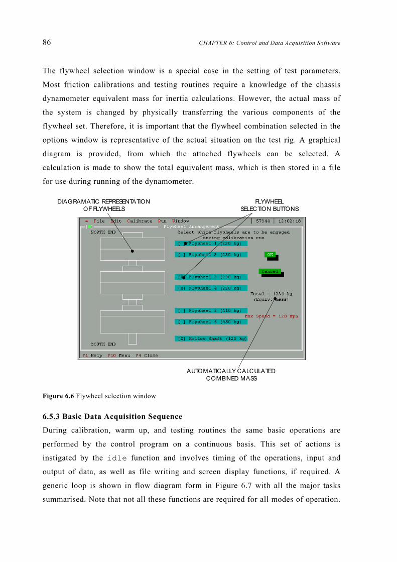
86 CHAPTER 6: Control and Data Acquisition Software
The flywheel selection window is a special case in the setting of test parameters.
Most friction calibrations and testing routines require a knowledge of the chassis
dynamometer equivalent mass for inertia calculations. However, the actual mass of
the system is changed by physically transferring the various components of the
flywheel set. Therefore, it is important that the flywheel combination selected in the
options window is representative of the actual situation on the test rig. A graphical
diagram is provided, from which the attached flywheels can be selected. A
calculation is made to show the total equivalent mass, which is then stored in a file
for use during running of the dynamometer.
Figure 6.6 Flywheel selection window
6.5.3 Basic Data Acquisition Sequence
During calibration, warm up, and testing routines the same basic operations are
performed by the control program on a continuous basis. This set of actions is
instigated by the idle function and involves timing of the operations, input and
output of data, as well as file writing and screen display functions, if required. A
generic loop is shown in flow diagram form in Figure 6.7 with all the major tasks
summarised. Note that not all these functions are required for all modes of operation.
DIAGRAMATIC REPRESENTATION OF FLYWHEELS
AUTOMATICALLY CALCULATEDCOMBINED MASS
FLYWHEEL SELECTION BUTTONS

6.5 Control Program Functionality 87
Specific exclusions or additional items of interest are included in Sections 6.5.4–
6.5.12.
Before any operations involving running of the chassis dynamometer, several
equipment checks are made to ensure that the correct modes are engaged, and that the
water and compressed air pressures are sufficient. These checks make use of sensors,
which are wired to the PCLD-782 digital-input daughter board and depend on what
type of dynamometer running is required. The user may be prompted to correctly set
any of the following parameters before the program will continue: Main panel on/off,
ASEA motor mode, Froude dynamometer panel on/off, dynamometer mode,
dynamometer over-speed, dynamometer water valve, axle brake air valve, axle oil
heater, or exhaust fan on/off. This checking routine is included as ModeCheck in the
file UTILITY.CPP.
6.5.3.1 Timing
As mentioned in Section 6.5.1, the updating data acquisition routine is called as a
result of the idle function, which only functions if there are no other program tasks
awaiting processor time. Thus, the time taken outside the routines shown in Figure
6.7 may vary depending—for instance—on whether there were any keyboard events
to handle since the last time the data acquisition sequence was called. To enable the
accurate timing of data capture and D/A demands, the UPP card is used to generate
an interrupt every 4.75 µs, which is counted by the software and used to set a flag at
0.1s or 0.2s intervals (4.75µs×421×50 = 0.099999 sec). Regardless of the time taken
outside the update routine, once the timing loop is entered, the program is delayed
until the next time interval is reached (indicated by the state of the software flag).
An exception occurs if the time taken by the update loop added to the time taken by
the external processes exceeds the prescribed time interval. In this case, a time error
record is generated, and no significant time is spent in the waiting loop. To avoid
such instances, a record of the wait-time is generated each time through, and
displayed on screen as well as being saved to the file (if needed). This delay function
records the time at which the wait loop was entered and when it was exited, thus
giving the total amount of time that was spent waiting. This figure is presented as a

88 CHAPTER 6: Control and Data Acquisition Software
Figure 6.7 Flow diagram of basic data acquisition routine
percentage of the total available time interval (0.1s or 0.2s) and was most useful
during creation of each routine and debugging to determine the ideal time interval to
set, and which tasks were consuming the most processor time.
6.5.3.2 Data Inputs
Each of the A/D channels in use on the PCL-812PG card has a corresponding group
of settings in the configuration file, as described in Section 6.3.1. All the PCL-812PG
Next Time Interval
Reached ?
Read A/D data in
NO
YES
Send D/A Demands
Perform Calculations
Update Display
Write to File
Recording Data ?
YES
NO

6.5 Control Program Functionality 89
channels are read in a single step, using the appropriate gains from this configuration
file. Several channels, such as the thermocouple inputs to the PCLD-889 daughter-
board and the Annubar pressure transducers require more than a simple linear
relationship to relate the voltage signal to the correct units for the data (see
calibration Appendix C). All calculations are performed on the raw data immediately
after being read, and the results are displayed and stored in the correct units only, as
opposed to the original digital bits or their corresponding voltages.
Two important data inputs are derived from sources other than the PCL-812PG and
PCLD-889 cards. The rotational velocity (and hence drum surface speed) as well as
the engine speed (rpm) are both found using pulse counting and timing routines with
the UPP card, as detailed in Section 4.1. As soon as the timing delay loop is exited,
the number of shaft encoder and engine spark pulses counted since last time are read
in. With knowledge of the time and number of pulses, the speeds can be calculated
using the pulse counting method of Equation 4-1. Note that the vehicle data file must
include the number of sparks generated per engine revolution so the spark speed can
be converted to engine revolutions-per-minute.
In the case where the allotted loop time is exceeded (see Section 6.5.3.1) the time
taken before the number of pulses are read is greater than expected. This gives the
appearance of a rapid jump in speed, followed by a rapid decrease, as the next time
through the loop is slightly shorter (meaning less pulses are counted). Errors can also
arise from the inductive loop that records spark plug pulses (see Appendix D).
Occasionally, an extra spark pulse is detected from one of the nearby leads, or a
single pulse is not detected by the circuitry. These pulse inaccuracies are brought
about by slight inconsistencies in the intensity of the spark plug current, and result in
significant fluctuations in the measured speed. Apparent jumps in roller and spark
speed are corrected for in the software by checking new speed values against the
previously recorded values. If a timing error is known to have occurred, or if an
implausible increase or decrease in speed is measured (e.g. >2000 rpm in 0.1s) the
new data is skipped and the previous data substituted in its place so that the speed
appears constant. Although this constant approximation may not be entirely accurate,
is it superior to including large errant speed values.

90 CHAPTER 6: Control and Data Acquisition Software
Specific routines for reading A/D values, calculating thermocouple temperatures, and
determining speed from pulses can be found in the source code in file
DATA_AQ.CPP.
6.5.3.3 Power Calculation and Atmospheric Correction
Vehicle output power is an important test parameter that cannot be directly measured,
and may be calculated in one of several different ways. Power is defined as the
product of force and velocity. In this case, the force at the roller surface can either be
measured using the tractive effort load cell, or assumed, given the sum of the
resisting forces.
vFPower corr= (6-3)
Where: Fcorr = Raw tractive effort + Correction (as per Equation 5-14)
vFFdtdvmPower fricdynocd
++= (6-4)
Experiments were carried out on both methods, and it was decided that using the
tractive effort load cell was more appropriate, particularly when acceleration was a
factor. Although the dynamometer load cell tended to exhibit greater accuracy and
less hysteresis, Equation 6-4 requires that the acceleration be multiplied by the total
equivalent mass, as opposed to the mass of the drum assembly only in Equation 6-3.
This means any error in the determination of acceleration (see Section 5.2) would
induce a greater error in the final calculated power when using Equation 6-4.
Once the force and velocity at the drum surface have been measured, it is necessary
to standardise these measurements to account for atmospheric conditions. Changes in
air temperature and pressure can have a significant effect on vehicle performance,
particularly in relation to the density of the air entering the engine. Equation 6-5
shows the standard power correction, which is carried out each time through the data
acquisition loop. If desired, on-road fuel consumption figures may also be corrected
to account for atmospheric conditions [SAE J1082, 1995].
6.5 Control Program Functionality 91
std
m
m
stdmcorr T
TppPP
= (6-5)
Where: Pm = power calculated from force and velocity (W)
pm = measured air pressure (kPa)
Tm = measured absolute air temperature (K)
pstd = standard atmospheric pressure (1013kPa)
Tstd = standard atmospheric absolute temperature (293K)
Also of interest is the power output of the vehicle referenced to the engine flywheel.
This can be loosely approximated as the power output at the road wheels less the
rolling and transmission frictions, which is measured during a coastdown on the
dynamometer (Section 5.4). An engine power approximation of this sort is offered as
an option in the MATLAB post-processing software discussed in Chapter 7.
6.5.3.4 Data Outputs
Depending of the mode of operation of the chassis dynamometer, the power absorber
may be controlled in speed or torque mode. ‘Power law’ control is available, but is
not generally used in chassis dynamometer applications. The electric motor can also
be switched between speed and torque control using the digital output capability of
the PCL-812PG. The required demand is calculated in terms of useful units (kph for
velocity, and Nm for torque), which must be converted to a 12-bit integer for use by
the A/D card. The PCL-812PG receives this number and applies a proportional
voltage output. The linear equations to convert from useful units to the appropriate
12-bit integer are included in the configuration file (see Section 6.3.1), as are
appropriate upper and lower limits for the demand output. Each output voltage is
applied to the motor or dynamometer as a constant demand requirement, which is
acted upon by the built-in analogue control circuitry (see Section 2.5.1). D/A demand
calibration details are included in Appendix C.
6.5.3.5 Text Display
Text is displayed on screen and updated each time through the loop so the user can
track the progress of warm up or testing procedures. Before a test can begin, the
screen display is initially set up with all the necessary buttons as well the data labels
92 CHAPTER 6: Control and Data Acquisition Software
and units that do not change throughout the operation. Data labels, such as ‘Roller
Speed’ are again stored in—and retrieved from—the configuration file. Once the
routine is running, data is read (as per Section 6.5.3.2) and displayed on screen in a
similar way to how it is written in the file. A special text class was created to enable
the efficient updating of this data, without flickering or delays in the display. Each
mode of operation has a similar on-screen appearance, with some variation in the
amount of data and button options that are available. The major exception is the
‘Driving Cycle’ mode, which dispenses with the Turbo Vision format to enable an
efficient and highly visible scrolling display (see Section 6.5.12.1). Refreshing the
Turbo Vision screen display is a relatively time-consuming process and in some cases
this dictates the updating rate (set by the time interval as per Section 6.5.3.1). The
slower timing rate of 0.2s is used for ‘Road Load Driving’, ‘Manual Control’ and
‘Warming Up’ where on-screen user feedback of all measured parameters is more
important than the rate at which data is saved.
6.5.3.6 File Saving
As discussed in Section 6.3.2, test data may be saved to a file specified in advance by
the user. A complete set of data is written to the save file each time the updating
routine is executed, provided that the program is in a recording phase. Data may be
saved continually when under ‘Manual’ or ‘Road Load’ control, and is always saved
in ‘Driving Cycle’ mode. Averaged data values are stored in the file only at specific
points during mapping tests. All the A/D data and external inputs such as roller and
engine speeds are temporarily stored in a numerical array as they are received, then
the entire array is written to the predefined file at the end of each updating sequence.
In addition, several other pieces of information, such as the latest calculated
acceleration and power, and the power absorber demand, are transferred from
separate arrays into the file each time through the loop.
The computing time required for file transfer operations can—in some cases—
become restrictive, since the correct location on the hard drive must be accessed each
time by the scanning head. If additional operations were added to the data acquisition
loop, different ways of saving the input data may need to be implemented. One such
technique is to write the data from an array into the computer’s random-access

6.5 Control Program Functionality 93
memory instead of into a file on the hard disk. Further information on this option is
included in Section 9.2.
6.5.4 A/D and D/A Calibration Function
The chassis dynamometer control program includes a simple, multi-purpose routine
designed for calibration of the various PCL-812PG inputs and outputs. The
calibration program displays a text-only (DOS format) screen with the necessary
prompts, and reads the desired channels applying user-defined settings. Instead of
reading the A/D settings from a configuration file, the user is prompted for all the
important information such as which channel to use, the gain to set, and how many
samples to average each time.
During A/D calibration, a known magnitude is applied to the appropriate device (e.g.
a known force on a load cell) and the user enters this value on the keyboard.
Acceptance of this entry initiates sampling of the desired channel, and the voltage
and 12-bit integer (0–4095) representation are both stored in a file. After several
different points have been recorded, the user exits and the mathematics routines as
described in Section 6.4 are used to calculate a linear or quadratic relationship
between the known entries and the A/D reading. This equation is then displayed and
saved to a file, from which the coefficients can be copied into the configuration file
for future use during testing.
Digital to analogue calibrations operate in much the same way, but rather than a
known quantity being supplied, the user enters a series of 12-bit numbers as inputs to
the PCL-812PG. Depending on the mode of operation selected by the user, this 12-bit
integer entry sets the voltage for the speed or torque controller on either the electric
motor or the power absorber. Once a steady state is reached on the control output, the
user presses a key, which stores the combinations of raw entry and final output.
Again, a least squares approximation is performed so that when in use, the required
value (e.g. torque in Nm) can be related to the 12-bit D/A input that will set the
correct controller voltage.

94 CHAPTER 6: Control and Data Acquisition Software
Figure 6.8 Screenshot of D/A calibration display
6.5.5 Friction Calibration Function
As mentioned in Section 5.4, the frictional characteristics of the chassis
dynamometer system are likely to change over time. For this reason it was necessary
to have a simple procedure to follow that would measure the friction forces and
calculate the current coefficients of the system as whole, and the drum assembly in
isolation. Friction calibrations should be carried out both with a vehicle in place, and
with the chassis dynamometer alone, so the appropriate forces can be used in road
load calculations as well as correction of the raw tractive effort load cell signal, as
per Equation 5-16.
Best results are obtained by running a series of coastdowns, and averaging the
solution of Equations 5-13. Various options can be set to ensure accurate and
repeatable data. Choices include: maximum and minimum speed of coastdown, how
many runs to perform, and the desired dynamometer torque for each. On-screen
display during the coastdown process includes velocity, dynamometer torque, tractive
effort, and timer, as well as ‘Start’, ‘Accept’, ‘Redo Run’, and ‘Exit’ buttons. Each
coastdown starts with the electric motor accelerating the chassis dynamometer (with
vehicle in neutral, if present) to a point approximately 15 kph above the maximum
recorded coastdown velocity. At this point, the motor load is removed and the
D/ A DEMAND ENTERED IN BITS (0-4095)
CURRENT SPEED AND TORQUES
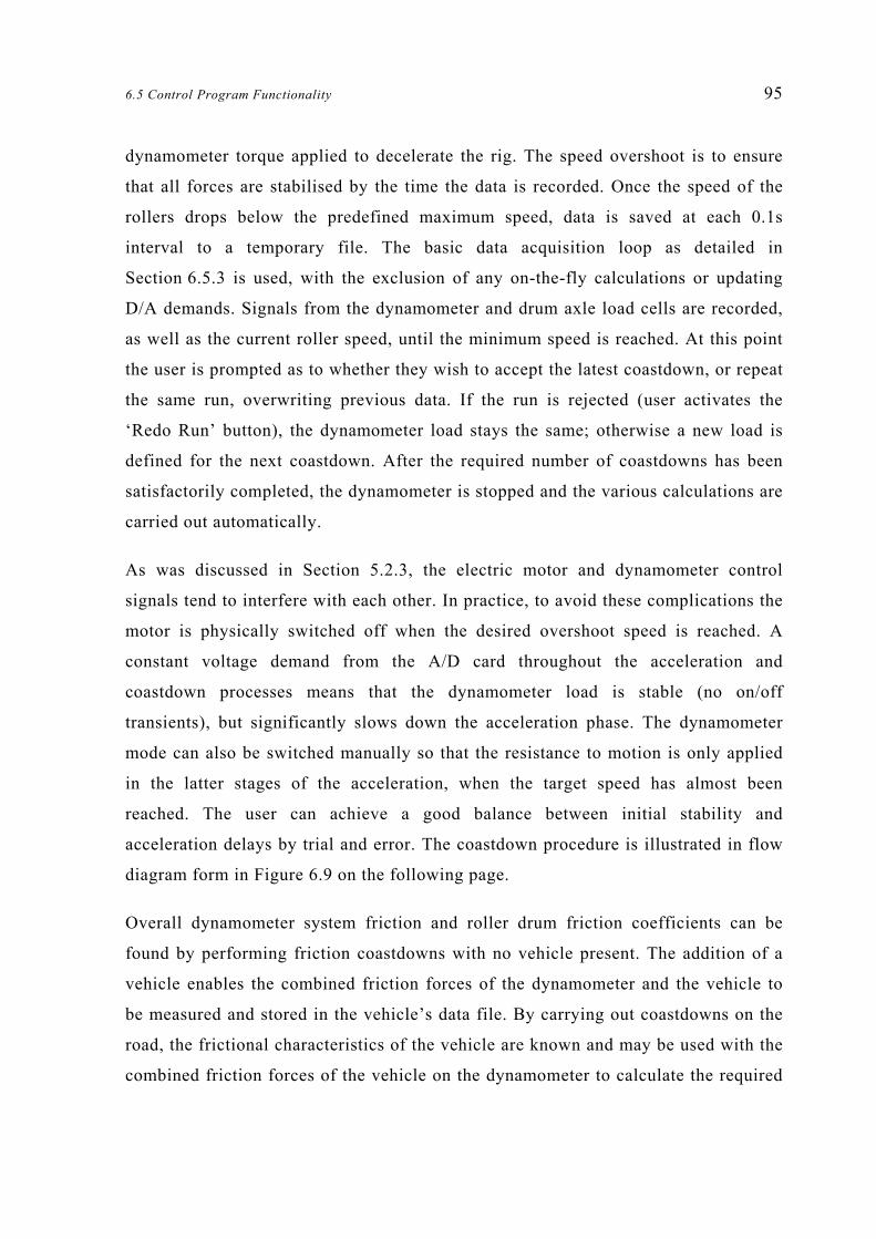
6.5 Control Program Functionality 95
dynamometer torque applied to decelerate the rig. The speed overshoot is to ensure
that all forces are stabilised by the time the data is recorded. Once the speed of the
rollers drops below the predefined maximum speed, data is saved at each 0.1s
interval to a temporary file. The basic data acquisition loop as detailed in
Section 6.5.3 is used, with the exclusion of any on-the-fly calculations or updating
D/A demands. Signals from the dynamometer and drum axle load cells are recorded,
as well as the current roller speed, until the minimum speed is reached. At this point
the user is prompted as to whether they wish to accept the latest coastdown, or repeat
the same run, overwriting previous data. If the run is rejected (user activates the
‘Redo Run’ button), the dynamometer load stays the same; otherwise a new load is
defined for the next coastdown. After the required number of coastdowns has been
satisfactorily completed, the dynamometer is stopped and the various calculations are
carried out automatically.
As was discussed in Section 5.2.3, the electric motor and dynamometer control
signals tend to interfere with each other. In practice, to avoid these complications the
motor is physically switched off when the desired overshoot speed is reached. A
constant voltage demand from the A/D card throughout the acceleration and
coastdown processes means that the dynamometer load is stable (no on/off
transients), but significantly slows down the acceleration phase. The dynamometer
mode can also be switched manually so that the resistance to motion is only applied
in the latter stages of the acceleration, when the target speed has almost been
reached. The user can achieve a good balance between initial stability and
acceleration delays by trial and error. The coastdown procedure is illustrated in flow
diagram form in Figure 6.9 on the following page.
Overall dynamometer system friction and roller drum friction coefficients can be
found by performing friction coastdowns with no vehicle present. The addition of a
vehicle enables the combined friction forces of the dynamometer and the vehicle to
be measured and stored in the vehicle’s data file. By carrying out coastdowns on the
road, the frictional characteristics of the vehicle are known and may be used with the
combined friction forces of the vehicle on the dynamometer to calculate the required
z
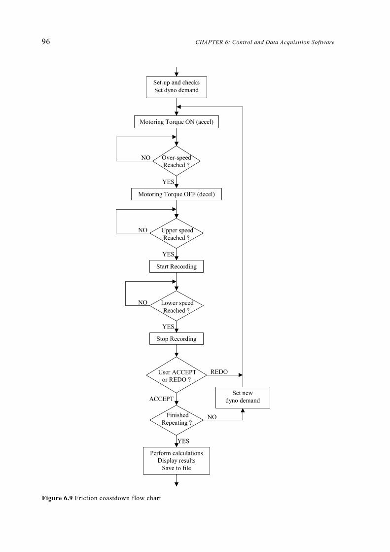
96 CHAPTER 6: Control and Data Acquisition Software
Figure 6.9 Friction coastdown flow chart
Set-up and checksSet dyno demand
Motoring Torque ON (accel)
Over-speed Reached ?
NO
Motoring Torque OFF (decel)
Upper speed Reached ?
NO
YES
YES
Start Recording
Lower speed Reached ?
NO
YES
Stop Recording
User ACCEPT or REDO ?
Set new dyno demand ACCEPT
REDO
Finished Repeating ?
YES
NO
Perform calculationsDisplay results
Save to file

6.5 Control Program Functionality 97
road load power absorber torque as per Equation 3-10. Roller drum friction is used to
correct the tractive effort load cell reading as detailed in Section 5.5, while the
frictional resistance of the dynamometer alone may be used to approximate the
vehicle power output at the engine flywheel as follows. The transmission and rolling
friction of a vehicle on the dynamometer is calculated as the friction of the vehicle
and the dynamometer combined, less the friction of the dynamometer alone.
( ) ( ) ( ) 2221100 vffvffffF dVddVddVdVf −+−+−= (6-6)
Where: FVf = transmission and rolling friction of vehicle on dynamometer
Other notation as per Nomenclature section
Therefore, the power generated at the engine flywheel is approximated as the power
output at the road wheels (measured by the tractive effort load cell) plus the frictional
power absorbed by the vehicle transmission, driveshaft and tyres.
( )vFFP VfVeng += (6-7)
Where: Peng = engine power referenced to the flywheel (W) which may then be
corrected for atmospheric conditions (see Equation 6-5)
FV = tractive force at roller surface (N)
The actual determination of each set of frictional coefficients is carried out
immediately after exiting the coastdown routine, and the specific calculations depend
on whether a vehicle was present on the rollers or not. All the necessary data is saved
to a file, from which arrays are generated for use by the mathematics functions
mentioned in Section 6.4. Measured data is replaced by least squares approximations,
which are then used to generate systems of equations for the simultaneous solving of
Equation 5-12. These coefficients are in turn stored in the appropriate file.
Dynamometer system and drum friction characteristics are automatically saved in a
file whose name includes a numerical representation of the particular dynamometer
flywheel combination in use at the time. This is because the system friction as a
whole changes depending on which flywheels are engaged, and which are spinning
on their shaft bearings (see Section 5.4). The combined vehicle and dynamometer

98 CHAPTER 6: Control and Data Acquisition Software
friction is saved in the data file of the vehicle indicated by the user, so that the
appropriate frictional forces will be loaded next time the same vehicle is used. When
calibrating dynamometer and vehicle friction, it is important to engage the flywheel
combination most appropriate to the vehicle so that the calculated coefficients can be
used for tests that involve road load simulation with these flywheels.
Friction coastdown theory and examples of the repeatability of the system friction
and drum friction methods are included in Sections 5.4 and 5.5.2 respectively.
Graphs of velocity, acceleration, dynamometer torque, and tractive effort during a
friction coastdown run are included as an example in Appendix S.
6.5.6 Re-zeroing Load Cells
As described in Section 4.3.1, the dynamometer and tractive effort load cells were
affected by temperature and required regular re-zeroing. Simple routines were
devised to find the appropriate offsets for the tractive force and power absorber
torque readings before each batch of testing.
For the dynamometer load cell, the user is prompted to push down briefly on the
appropriate load arm (depending on the desired direction of rotation) to remove the
hysteresis, then by hitting the ‘Accept’ button the A/D 12-bit reading is recorded at
this zero load. Because the power absorber always applies a force which opposes the
direction of motion, the hysteresis is best accounted for by applying the initial
loading in the load direction only. This 12-bit integer is stored as a global variable, as
well as in a file, and is reloaded before any testing is carried out. During testing, the
offset obtained during re-zeroing is subtracted from the raw A/D value read from the
load cell, and then the predefined linear multiplier (from the configuration file) is
applied.
In the case of the tractive effort load cell, loading can occur in both directions, so the
user is prompted to apply a small load (≈50 N) to the load arm, first in the positive
direction and then in the negative direction. The zero point is taken as the average of
these two small readings and again is stored as a global variable and in a file for use
during testing.
6.5 Control Program Functionality 99
6.5.7 NOX Meter Setup
The University of Canterbury Mechanical Engineering Department possesses a suite
of exhaust emissions measuring equipment for the purpose of engine and vehicle
testing. Separate Beckman devices to measure CO, CO2, NOX and unburnt
hydrocarbons are all available. However, due to time constraints in the present
project, only one of these was reinstalled for use with the chassis dynamometer. The
Beckman NOX meter (Model 951A), detects oxides of nitrogen (NO and NO2) in a
given sample and outputs the concentration via an analogue needle gauge on the
equipment and a 0–5 V output that can be read by the PCL-812PG. Setting up of the
NOX equipment involves first passing a ‘zero gas’ through the meter to ascertain the
zero concentration reading, then passing a ‘span gas’ of known concentration through
to check that the near maximum reading is correct. Trim knobs are used to obtain the
desired reading with zero and span inputs.
The software routine to assist this initial calibration consists of a single display
window, which shows the current voltage output, the previous zero and span
voltages, and buttons to accept zero and span gas readings. The user is also able to
enter the span gas concentration and the range to be used during the span reading, as
well the range to be used during subsequent testing. In terms of the basic data
acquisition loop (Figure 6.7), the major differences are that there are no D/A
demands and that the data recording is only performed as a one-off upon use of the
‘Zero Accept ‘or ‘Span Accept’ buttons.
While the zero gas is passed through the device, the most sensitive range setting is
chosen and the trim should be adjusted to provide a zero volt output to the A/D card.
A suitable range should then be chosen and indicated on-screen to most closely
approximate the particular span gas concentration in parts per million (ppm). For
example, the 0–2500 ppm range (the actual figures are only a guide) could be used
with 3000 ppm span gas, with a full 5 V then representing 3000 ppm. The span gas
concentration entered by the user is utilised during subsequent testing to calculate
concentrations depending upon the range setting indicated in this window. For
example, if a 3000 ppm span gas was used on the 2500 ppm range setting, and testing

100 CHAPTER 6: Control and Data Acquisition Software
was to be carried out using the 10000 ppm range setting, the following factors would
be calculated and applied to the sample voltage during testing.
CONCSPANRANGESPANRANGETEST
VOLTAGESPANVOLTAGETESTCONCTEST ××= (6-8)
For example, during testing:
SPAN RANGE = 2500 ppm TEST RANGE = 10000 ppm
SPAN VOLTAGE = 5 V TEST VOLTAGE = 2.5 V
SPAN GAS CONC = 3000 ppm
ppmCONCTEST 600030002500
1000055.2
=××=
The combination of span range, test range, span voltage, and span gas concentration
is stored as a single variable which can be applied to each A/D voltage during testing
to provide an output in parts per million.
6.5.8 Warm Up Routine
The frictional characteristics of gears and bearings vary greatly with operating
temperature, and it is therefore necessary to ensure that these temperatures are
consistent during any chassis dynamometer testing. The easiest way to achieve stable
component temperatures is to spin the rotating machinery at a high enough speed
until the inherent friction produces approximately the same amount of heat as is
radiated out or removed by the cooling system. A built-in timer can be implemented
to stop the warm up after a certain time interval, or alternately the user may simply
watch some of the temperature sensors and manually conclude the warm up when a
certain level is reached. During a warm up, the screen display shows all the available
sensors, including temperature measurements of the roller drum axle oil, the vehicle
engine oil and cooling water (if these thermocouples are installed). Figure 6.10 shows
a typical warm up window.
The warming up process may be carried out in one of three ways. ‘Constant Speed’
uses the electric motor to maintain a predefined set speed, while the ‘Road Load’
warm up option allows the user to accelerate and decelerate a vehicle against a road
z

6.5 Control Program Functionality 101
Figure 6.10 Warm up screen display
load model, which employs user-defined friction coefficients. ‘Manual Warm Up’ is
an option in which the D/A capability is not employed and the user operates the
electric motor and power absorber by physically manipulating the potentiometers and
mode buttons on the respective equipment panels. The timer—and any automatic load
demand—is set when the ‘Start’ button is activated and ceases if the allotted time has
elapsed, or if the user stops the procedure.
The optimum format and duration of a warm up can be arrived at by experience, and
depends on the type of testing and the vehicle. One way to determine whether the
dynamometer has reached an ideal operating state is to carry out a series of friction
calibration runs, observing changes in the frictional force at a certain velocity. A
calculated friction which is consistent between runs indicates that the temperature is
stable. Several trials were conducted to determine an appropriate speed and duration
for the constant velocity warm up. The results of two of these trials are graphed in
Appendix T. Initial running of 15 mins at approximately 50 kph, followed by a
shorter period at 100 kph was expected to result in stable frictional characteristics for
EQUIPMENT MONITORING
SPEEDS (UPP CARD) AND A/ D INPUTS (PCL-812PG)
TEMPERATURES AND PRESSURES (PCLD-889)
IDLE TIME PER CYCLE
MOTOR AND DYNO DEMAND (IF AUTOMATIC
CONTROL IS USED)

102 CHAPTER 6: Control and Data Acquisition Software
the dynamometer with no vehicle in place. However, a short break of one or two
minutes between warming up and testing may create variations in performance. It
should be noted that even relatively large changes in bearing friction usually equated
to less than 5 N force with respect to the drum surface, which was not serious in light
of the other system inaccuracies.
6.5.9 Manual Control
‘Warm Up’, ‘Road Load Driving’, and ‘Manual Control’ are all instances of the same
DisplayDialog class. This dialog box displays all the available A/D data as well
as several equipment states such as the electric motor and power absorber modes, and
whether or not there is sufficient air pressure for the axle brake, or water pressure for
the dynamometer. Each of these three operating modes follows the basic data
acquisition sequence, with similar appearances on screen. The major differences are
that the ‘Warm Up’ option does not include the buttons or capability for recording
data, and that the ‘Manual Control’ (distinct from the ‘Manual Warm Up’) mode
provides user input boxes to set the D/A demands for the eddy-current dynamometer
and electric motor. Each of the DisplayDialog functions samples data and
updates demands at the slower rate of 5 Hz to allow for all the data acquisition and
screen display operations.
The ‘Manual Control’ screen allows the user to switch the demand modes and
magnitudes for both the motor and the power absorber, which is useful for
investigation of the dynamometer performance and for flexible vehicle testing,
including maximum power runs (as recorded in Section 8.2.2). Either the mouse or
keyboard can be used to navigate about, and new D/A demands (in the correct units)
can be typed in the appropriate box and sent to the equipment by pressing the Enter
key, or activating the ‘Accept’ button. At any point, the current A/D data may be
recorded to a file, which is chosen by the user before entering the ‘Manual Control’
routine. ‘Snapshot’ (see Figure 6.11) saves all the data at a single instant, while
‘5 sec Record’ records the data in the file at 0.2 second intervals for 5 seconds.
Provision is made for the user to change the duration of recording to anything
between 0 and 10 seconds. ‘Record ON’ simply starts saving data at each interval and
z
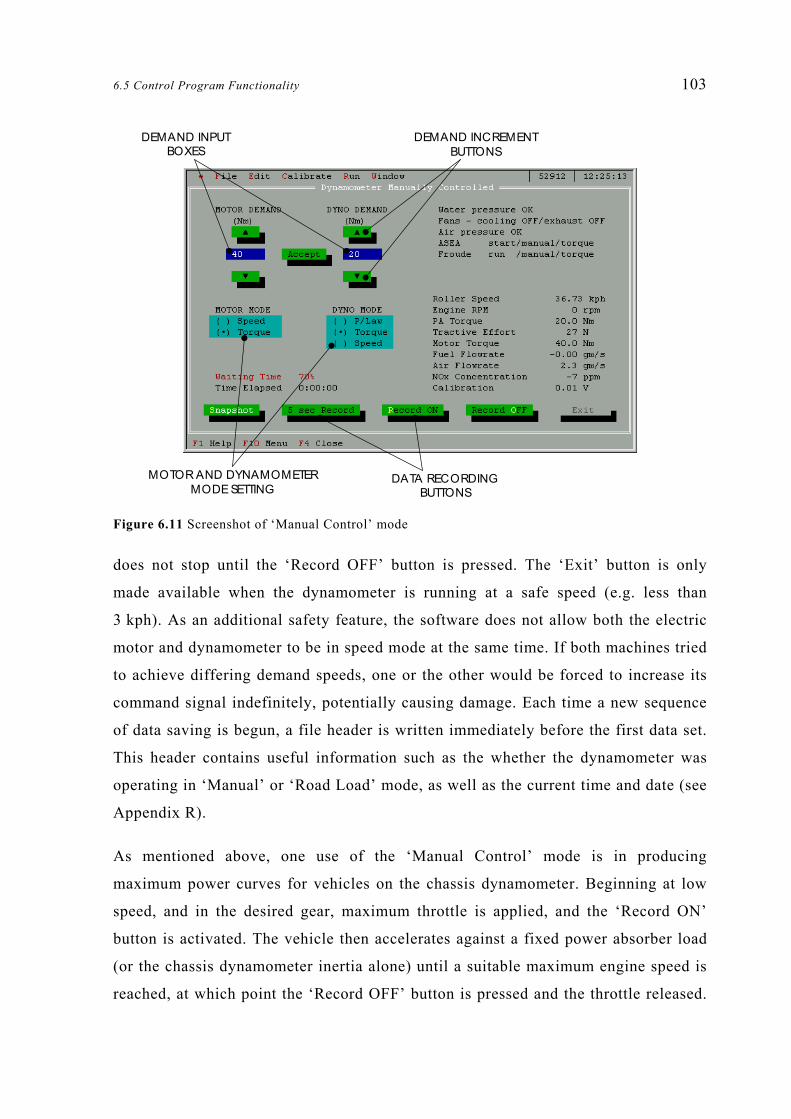
6.5 Control Program Functionality 103
Figure 6.11 Screenshot of ‘Manual Control’ mode
does not stop until the ‘Record OFF’ button is pressed. The ‘Exit’ button is only
made available when the dynamometer is running at a safe speed (e.g. less than
3 kph). As an additional safety feature, the software does not allow both the electric
motor and dynamometer to be in speed mode at the same time. If both machines tried
to achieve differing demand speeds, one or the other would be forced to increase its
command signal indefinitely, potentially causing damage. Each time a new sequence
of data saving is begun, a file header is written immediately before the first data set.
This header contains useful information such as the whether the dynamometer was
operating in ‘Manual’ or ‘Road Load’ mode, as well as the current time and date (see
Appendix R).
As mentioned above, one use of the ‘Manual Control’ mode is in producing
maximum power curves for vehicles on the chassis dynamometer. Beginning at low
speed, and in the desired gear, maximum throttle is applied, and the ‘Record ON’
button is activated. The vehicle then accelerates against a fixed power absorber load
(or the chassis dynamometer inertia alone) until a suitable maximum engine speed is
reached, at which point the ‘Record OFF’ button is pressed and the throttle released.
DEMAND INPUT BOXES
DEMAND INCREMENT BUTTONS
MOTOR AND DYNAMOMETER MODE SETTING
DATA RECORDING BUTTONS

104 CHAPTER 6: Control and Data Acquisition Software
On-the-fly calculations of power using the tractive effort load cell reading as per
Section 6.5.3.3 can then be plotted against road or engine speed. The MATLAB
routines detailed in Section 7.1.3.1 enable a superior plot to be produced by filtering
the acceleration (and hence power) in a way which cannot be performed during the
testing.
6.5.10 Road Load Driving
The ‘Road Load Driving’ function also uses the DisplayDialog class and screen
display. The purpose of this routine is to run a vehicle under on-road conditions with
respect to velocity-dependent friction, and inertial loads. The display is similar to
that used for the ‘Warm Up’ procedure, except that it includes recording buttons, and
does not require ‘Start’ or ‘Stop’ functions. For safety reasons, the user may exit this
screen only when the roller speed is less than a predefined level (e.g. 3 kph).
The only readily adjustable parameter in ‘Road Load’ mode is the duration of the
preset recording interval (shown as 5 seconds in Figure 6.11). The selection of the
flywheel configuration and correct vehicle file are important for achieving realistic
road load simulation. The combined inertia and frictional characteristics required to
implement Equation 3-10 are retrieved from files before running. At all times while
the display screen is visible, the basic loop of Section 6.5.3 is carried out at each
0.2 second interval and a new power absorber torque demand is calculated and sent
via the PCL-812PG. The electric motor is generally switched off to avoid any
unwanted torque blips or interference with the load cell signals.
Because the ‘Road Load Driving’ function applies a dynamometer load in the same
way as the ‘Driving Cycle’ mode, it is useful for familiarising a human driver with
the feel and response of the chassis dynamometer and vehicle before undertaking
thorough testing. Also, investigations may be made into the appropriateness of
certain velocity demand sequences that are not yet available as driving cycle files.
Perhaps the most useful application of the ‘Road Load Driving’ routine is in
recording the fuel consumption at constant speed under simulation conditions. These
constant speed consumption values are usually quoted in km/litre and provide a
standardised comparison between vehicles.

6.5 Control Program Functionality 105
6.5.11 Mapping Test
The mapping test is a steady state examination of a vehicle’s performance over a
wide range of speeds and engine loads. It is useful for comparing one vehicle with
another, or to determine the results of any tuning or alterations made to a single
vehicle. The vehicle under test is driven on the dynamometer at a series of speeds,
and at each speed undertakes a series of tractive effort loads, resisted by the power
absorber. Some of the most useful measurements to be made are those of fuel
consumption, exhaust emissions, and efficiency at each set point.
The University of Canterbury chassis dynamometer conducts mapping tests under
speed control from the dynamometer, with the driver of the vehicle being required to
match the desired tractive effort load by application of the accelerator pedal. All
mapping tests are carried out in a single gear, which depends on the range of engine
speeds to be investigated. After thoroughly warming up the vehicle and chassis
dynamometer, and with the power absorber in speed control mode, the driver
accelerates to the predetermined maximum speed, at which point the dynamometer
holds the velocity constant. The driver then attempts to match the desired tractive
effort load (indicated on screen, and measured at the drum axle load cell) with the
accelerator. The minimum tractive effort load is largely determined by the stability of
the power absorber controller at the lower end of its range. Once the minimum load
has been achieved in a stable fashion, the user allows all the measured data inputs to
be saved, and the next (increased) load is shown on screen. The driver continues to
match the increased demands, while the dynamometer holds the rollers at a constant
rotational velocity. When the maximum force output at that speed is reached (i.e.
constant tractive effort at full throttle) this data is again saved and the next speed
demand is sent to the power absorber. The intervals with which desired tractive effort
is incremented and speed control is decremented are determined beforehand in the
mapping test configuration window. The mapping test ends when the user decides
that the vehicle can no longer maintain a constant speed in the current gear without
excessive instability or possibility of engine stall. The ‘Mapping Test’ sequence is
represented in flow diagram form in Figure 6.12. Note: Tractive Effort is abbreviated
as T.E.

106 CHAPTER 6: Control and Data Acquisition Software
Figure 6.12 Flow diagram of mapping test procedure
The driver is presented with on-screen feedback about the current speed and tractive
effort, with information on the average values, and fluctuations away from these
averages. It is important that the load and speed are both stable and constant at each
set point before the data is saved, and the display can be set up to indicate this
stability by changing the colour of the text. Green text indicates that the measured
Set-up and checks Dyno speed demand = maxDesired vehicle T.E. = min
Driver brings vehicle to demand speed
YES
NO
User accept desired
T.E.?
User accept max.
T.E.? NONO
Minimum speed
recorded ?
YES YES
Write data to file
Increment T.E.
Write data to file
Set minimum T.E.
Set new dyno speed demand
YES
NO
Can the desired T.E. be
achieved ?

6.5 Control Program Functionality 107
parameter has remained within preset fluctuation limits for a predetermined length of
time. For example, the user might set in the configuration window that the tractive
effort should not vary by more than 10 N from each set point and should remain
within this ±10 N for a period of 1 second. Once the desired stability is achieved, the
control program can be set to automatically record the data and move on to the next
set point. However, to allow for the idiosyncrasies of driver and power absorber
controls, and to accommodate some of the sensors which took longer to stabilise (see
Section 8.2.3.3) the ‘Accept’ button was manually applied when sufficient steadiness
had been achieved. An example of the on-screen display is shown in Figure 6.13,
including the green fluctuation indicator.
Figure 6.13 Screenshot of ‘Mapping Test’ display
This reduced display ensures greater clarity for the important parameters, and enables
the data loop to proceed at the increased rate of 10 Hz. Despite not being displayed,
all A/D channels are still sampled, averaged and saved to file when required. Because
of the requirement for constant speed and load, and the fact that data saving is not
required at each 0.1s interval, all measured data is saved as an average. The mapping
test configuration allows the user to set the interval over which these averages are
STABILITY INDICATOR AVERAGE OVER
LAST FEW TIME STEPS LATEST MEASURED
VALUE
INSTRUCTIONS TO GUIDE THE DRIVER

108 CHAPTER 6: Control and Data Acquisition Software
carried out (e.g. 0.5 secs = 5 readings averaged), and a record is kept of all the
necessary previous data points so that an average can be calculated and displayed on
screen, or saved to the file.
As well as all the A/D channels, the desired tractive effort and speed demand are
saved to the file, which is chosen by the user before commencement of the test. The
maximum load achieved by the test vehicle for each speed is unlikely to lie exactly
on one of the desired load steps. When the maximum vehicle tractive effort is
between intervals, the stability indicator will not activate (turn green), and a ‘-1’ is
added to the file in place of the desired tractive effort as a reminder. Calculations of
power (corrected for atmospheric conditions) and corrected tractive effort are both
made with the assumption of zero acceleration, and are stored in the file at each set
point. The format of the save file is similar to that of the other functions, and
includes a date and time header at the start of each test data set. Commas between
each number, and a new row for each set point makes for simple reading using the
MATLAB routines detailed in Chapter 7.
It should be noted that there are other ways of reaching all the load and speed points
of the vehicle map. One possibility is to make use of the dynamometer torque mode,
meaning that the driver would control the constant speed requirement using the
accelerator. This is a more natural throttle function for most drivers and may prove to
be a superior technique. This method creates other difficulties and is discussed
further in Section 9.2.
6.5.12 Driving Cycle
The most realistic and repeatable way to assess a vehicle’s on-road performance is by
conducting a ‘Driving Cycle’ test on the chassis dynamometer. A driving cycle
consists of a series of desired velocities (and sometimes, vehicle gears), usually at
one second intervals, which—as a whole—attempt to approximate the on-road
accelerations and speeds undertaken by a vehicle under certain conditions. When
carried out on a dynamometer, is it important that all the inertial and friction loads
present on the road are simulated on the machine. A vast array of driving cycles
exists to model the traffic and road conditions in various countries in urban driving
conditions and on the open road. Research into the suitability of several of these
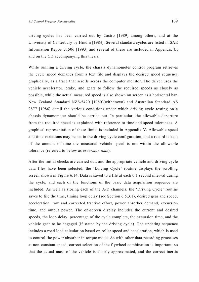
6.5 Control Program Functionality 109
driving cycles has been carried out by Castro [1989] among others, and at the
University of Canterbury by Hindin [1984]. Several standard cycles are listed in SAE
Information Report J1506 [1993] and several of these are included in Appendix U,
and on the CD accompanying this thesis.
While running a driving cycle, the chassis dynamometer control program retrieves
the cycle speed demands from a text file and displays the desired speed sequence
graphically, as a trace that scrolls across the computer monitor. The driver uses the
vehicle accelerator, brake, and gears to follow the required speeds as closely as
possible, while the actual measured speed is also shown on screen as a horizontal bar.
New Zealand Standard NZS-5420 [1980](withdrawn) and Australian Standard AS
2877 [1986] detail the various conditions under which driving cycle testing on a
chassis dynamometer should be carried out. In particular, the allowable departure
from the required speed is explained with reference to time and speed tolerances. A
graphical representation of these limits is included in Appendix V. Allowable speed
and time variations may be set in the driving cycle configuration, and a record is kept
of the amount of time the measured vehicle speed is not within the allowable
tolerance (referred to below as excursion time).
After the initial checks are carried out, and the appropriate vehicle and driving cycle
data files have been selected, the ‘Driving Cycle’ routine displays the scrolling
screen shown in Figure 6.14. Data is saved to a file at each 0.1 second interval during
the cycle, and each of the functions of the basic data acquisition sequence are
included. As well as storing each of the A/D channels, the ‘Driving Cycle’ routine
saves to file the time, timing loop delay (see Section 6.5.3.1), desired gear and speed,
acceleration, raw and corrected tractive effort, power absorber demand, excursion
time, and output power. The on-screen display includes the current and desired
speeds, the loop delay, percentage of the cycle complete, the excursion time, and the
vehicle gear to be engaged (if stated by the driving cycle). The updating sequence
includes a road load calculation based on roller speed and acceleration, which is used
to control the power absorber in torque mode. As with other data recording processes
at non-constant speed, correct selection of the flywheel combination is important, so
that the actual mass of the vehicle is closely approximated, and the correct inertia

110 CHAPTER 6: Control and Data Acquisition Software
simulation can be added by the dynamometer to make up the difference (as per
Equation 3-10).
6.5.12.1 Scrolling Display
The quality and form of the driving cycle display greatly affects the human driver’s
ability to follow it, and it was important that the system showed timely and correct
information in an intuitive way. For ideal driving cycle testing on a dynamometer,
the vehicle transmission and throttle are electronically controlled so that reaction
time and driver error are no longer factors. This type of system is readily available
and marketed by companies such as Schenck and Froude Consine. However,
satisfactory results may be obtained with experienced drivers, and computer control
of vehicles on the University of Canterbury chassis dynamometer is not planned in
the near future.
Figure 6.14 Screenshot of scrolling drive cycle display (white cycle trace scrolls from left to right)
Figure 6.14 shows a driving cycle in mid-action, with error band and gear indicator
visible. The tick marks on the vertical axis are set at 10 kph intervals, while the
horizontal axis markings show one second gaps. The demand speed (white) and the
TEST PROGRESS INDICATORS
SCROLLING DRIVE CYCLE TRACE
CURRENT TIME VERTICAL AXIS (10 KPH DIVISIONS)
CURRENT VEHICLE SPEED INDICATED BY HORIZONTAL
WHITE LINE
GEAR INDICATOR (ARROW PRE-EMPTS
CHANGE)
GREEN BAND INDICATES SPEED TOO LOW

6.5 Control Program Functionality 111
horizontal axis tick marks move from right to left at the rate of 10 pixels per second
(one pixel per update loop). The screen resolution enables 360 pixels in the
horizontal direction, and 480 vertically—including 350 within the graph boundaries.
The vertical axis in the centre of the screen indicates the current time, while the
narrow, white horizontal line is the current vehicle speed. The green band above the
current speed shows the difference between the desired and achieved velocities, and
indicates that the driver needs to increase the vehicle’s speed. A red band of the
appropriate thickness appears if deceleration is required to reach the present demand
speed. Each of these moving display units is placed using the draw_line or
fill_block commands (contained in MODEX.H) with the required colour. The
old pixels that no longer need to be displayed are then removed by substituting black
lines and blocks, so that the illusion of the line vacating one position and moving to
the next is maintained. The desired speed line is interpolated linearly to fill in the
vacant data points between each second of cycle data.
The purple block and ‘Test Progress’ percentage show the amount of time elapsed as
a proportion of the total cycle length. The gear indicator (showing [1]) uses a specific
routine to output large numbers according to the gears defined in the driving cycle
file, if these are provided. The gear selection routine (in TESTING.CPP) also reads
two seconds ahead in the cycle, so the driver can be warned of upcoming gear
changes. When a new gear demand is encountered in the file, the gear number is
alternately blacked out and made visible (i.e. flashes) while an arrow (shown to the
right of the number) indicates the direction of the gear change to be made (up, in the
case of Figure 6.14).
The current speed and gear are to be matched by the driver at the vertical centre axis.
However, several seconds of data must be recovered from the file in advance so that
the upcoming trace can be displayed to right of the vertical cursor. This lead-in time
enables the driver to anticipate the approaching speeds, and its duration may be
altered in the source code (TESTING.CPP). This advance data is stored in an
updating array and is also used to calculate whether the current speed is within the
predefined tolerances. Because the allowable deviations also include a time
component, the actual speed may anticipate or lag the desired speed changes and still

112 CHAPTER 6: Control and Data Acquisition Software
remain within the limits. For example, if the tolerances on speed were ±1 kph and
±0.5 sec an enlarged view taken from Figure 6.14 shows that although the desired
speed at the current instant is 13.9 kph (i.e. range = 12.9–14.9 kph), the desired speed
range 0.5 seconds ago was more like 11.6–13.6 kph, thus including the present
achieved velocity (see Figure 6.15). A more in-depth description of the tolerance
calculation is included in Section 7.1.4.
Excursion time (time spent outside the allowable limits) is calculated at each instant
by the C++ control program according to the user-defined tolerances. However, the
MATLAB post-processing software detailed in Chapter 7 can also be used to
calculate these deviations, and to substitute other tolerance limits after the driving
cycle test has been carried out.
Figure 6.15 Enhanced driving cycle plot showing allowable time tolerance
6.5.12.2 Dynamometer Tracking and Response During Driving Cycles
The power absorber torque is applied according to Equation 3-10, which makes use
of the current acceleration and speed, vehicle and dynamometer mass, and frictional
coefficients. The constant component of this friction force results in a non-zero
SPEED DEMAND TRACE
CURRENT VEHICLE SPEED
(12.0 kph)
CURRENT DEMAND SPEED
(13.9 kph)
CURRENT TIME
0.5 sec
1 kph

6.5 Control Program Functionality 113
torque demand even when the rollers are stationary. However, the design of the eddy-
current dynamometer is such that it cannot apply a torque at zero, or near-zero
speeds. Thus, the controller causes large current build-ups as the demand torque is
not achieved. Once motion begins again, a large overshoot occurs, resulting in an
inaccurate tractive force on the vehicle under test. Figure 6.16 shows the effect of a
non-zero torque demand on the stationary dynamometer, which is then accelerated by
a vehicle on the rollers.
215 220 225 230 235 240 245 250 255 260 265
0
10
20
30
40
50
60
70
80
Time (sec)
PA
Tor
que
(Nm
)
Desired Speed Dyno Demand Achieved Torque
Figure 6.16 Power absorber torque overshoot
A software adjustment was made to ensure that this current build-up did not
adversely affect driving cycle results. After the calculation of the required power
absorber load, an additional programming check is carried out to determine whether
the dynamometer is capable of delivering this demand torque. If the actual shaft
velocity is less than a preset limit, and the driving cycle is in a deceleration or
stationary mode, the power absorber demand is set to zero. By cutting out the demand
before zero speed is reached, the eddy current—which takes a finite time to
decrease—falls to zero just as the rollers are stopped. Figure 6.17 below shows a
deceleration, stationary period, and acceleration under the software-adjusted power
absorber demand.
The large overshoot shown in Figure 6.16 has been reduced by approximately 90%, at
the expense of an increase in lag. Delays when the dynamometer load was reapplied
were again due to the eddy-current response at low speed. This time-lag and
overshoot is less evident at higher speeds, and the accompanying error was thought to
be tolerable for driving cycle testing.

114 CHAPTER 6: Control and Data Acquisition Software
215 220 225 230 235 240 245 250 255 260 265-5
0
5
10
15
20
25
30
35
Time (sec)
Torq
ue (
Nm
) &
vel
ocity
(kph
)
Desired Speed Dyno Demand Achieved Torque
Figure 6.17 Power absorber torque with improved demand function
The current vehicle deceleration rate for determining the dynamometer cut-out is
ascertained from the ideal cycle speed demands, to ensure stable and repeatable
application and removal of power absorber load. For further dynamometer load
stability, the ideal acceleration (i.e. difference between adjacent driving cycle
demand speeds, divided by the time interval) may be substituted for the actual
calculated acceleration in the road load equation. Power absorber cut-out, tractive
effort correction, and road load calculation may each be carried out using this ideal
acceleration or the calculated acceleration, as discussed in Chapter 4. Satisfactory
results were achieved over several driving cycle tests (see Section 8.2.4) with the use
of ideal accelerations. Obviously, in ‘Road Load Driving’ mode there is no ideal
cycle to follow and the acceleration must still be calculated at each point in time.

CHAPTER 7:
Data Analysis and Presentation Software
7.1 Plotting and Analysis Software
A data analysis software package has been created using MATLAB for the purpose of
viewing and editing previously recorded chassis dynamometer data in a Windows
environment. A series of program files were written using MATLAB version 5.3,
making use of the matrix-based data storage structures and built-in graphical display
functions. These program files interact with each other and can be run by typing
viewdata at the MATLAB command prompt while in the correct directory. All
these so-called m-files (MATLAB files have the file extension *.m) are included on
CD and may be viewed with any text editor. The MATLAB analysis package is
menu-driven, providing the user with numbered options as shown in Figure 7.1.
Figure 7.1 Example of MATLAB screen display showing the available options and a user prompt

116 CHAPTER 7: Data Analysis and Presentation Software
7.1.1 Overview of MATLAB Functionality
The main menu allows the user to enter the submenus that control file selection,
graphing, editing raw data, and calculating additional data. Each of these (with the
exception of the data editing) has one or more m-files of its own. The overall menu
structure is summarised in tabular form in Appendix W. The file selection menu
allows the user to choose from any of the previously saved chassis dynamometer data
sets, and then loads all the information into matrices for use by the plotting and
calculating routines. The graphing routines enable plotting of the current data in a
variety of ways, and are discussed further in Section 7.1.3. Raw data editing simply
invokes a standard MATLAB function (keyboard) that enables all the current
variables to be viewed individually and edited using MATLAB command-line
entries. Additional data not saved by the C++ program—such as fuel consumption
(km/l), energy consumption (J) and efficiency (%)—may be found using the
‘Calculate Additional Data’ function. Also included in this section is the driving
cycle excursion calculation routine, which is discussed in full in Section 7.1.4. All
the options used to carry out the various plotting and calculation activities may be
altered by the user at will, and are stored in text files. Each time a particular menu is
arrived at, the previous settings are recovered from the predefined file for immediate
use or editing.
7.1.2 File Input/Output and Data Storage
The file structure produced by the C++ control program is such that it is easily read
using MATLAB file I/O functions. An example file is included in Appendix R, which
shows the divisions between the header and the data, and between each new data run.
Commas are used to separate consecutive text or numerical data. Each time a new
recording mode is entered in the control program (e.g. ‘Manual Control’, ‘Vehicle
Mapping’ etc) a new session is begun. Within each session, the user may start and
stop the recording of data several times, and each of these is referred to as a run.
Each session must have at least one run before it is saved to the file. Each saved
session contains a header with background information (e.g. current dynamometer
frictional coefficients) and title information (the name and units of each recorded
data channel). Each run is preceded by a date/time header, which includes the control
program mode, and driving cycle information if applicable. During the file selection

7.1 Plotting and Analysis Software 117
routine, the entire file is first scanned to count the number of asterisk dividers
(sessions) and equals-sign dividers (runs). Then the user enters the desired session
and run, and the file is again traversed, this time only until the desired run is reached.
At this point, consecutive data values are read (up to the end of the run) into a large
matrix, which contains all the numerical data, with each row containing all the input
channels at a single moment in time. The channel titles (e.g. ‘Roller Speed’) and
units (e.g. ‘kph’) are also stored in separate matrices. The same process is performed
when the MATLAB program is initially started up. The most recently used file,
session, and run are recovered and the appropriate data is stored in matrices ready for
use. These matrices are then passed between the m-files as required, so that the latest
data is available to all parts of the software. Checking and reading from data files can
be a relatively time consuming process. For example, a 390-second driving cycle file,
with 27 data columns recorded every 0.1 seconds takes approximately 17 seconds to
download into the appropriate matrices. However, once in matrix format, this
information can be transferred between m-files or set up for graphical display in less
than 1 second.
7.1.3 Plotting Functions
The primary function of the post-processing MATLAB programs is to display test
data in a flexible and easy-to-use format. The standard MATLAB plot function can
be used to plot any column in the data matrix against any other to observe trends
within a test run, or to compare two or more separate runs. The user chooses the x
and y data sets, as well as the colour of the line and whether the plot is to overlap or
replace the previous plot, or produce a new plot window. The titles and units matrices
are also accessed so that the axes are automatically labelled and the graph is provided
with a title. The MATLAB graphing environment also allows the appearance of the
plot area and text to be altered after plotting.
7.1.3.1 Plotting Power Curves
One indication of a vehicle’s performance is the maximum power produced at the
road wheels. Remaining in a single gear and accelerating under maximum throttle,
the peak force and power can be found and related to the corresponding engine or
road speed. Power curves are best performed under the ‘Manual Control’ mode (see

118 CHAPTER 7: Data Analysis and Presentation Software
Section 6.5.9) with a constant—or zero—dynamometer torque. By using the raw
tractive effort signal, the corrected tractive effort and power can be recalculated as
per Equations 5-15 and 6-5 using a smoother acceleration with zero lag. Because the
entire speed sequence is available (as opposed to on-the-fly calculations) and the
speed changes are relatively steady, the acceleration is calculated using a simple
central difference approximation.
T
vvv2
021
−=& (7-1)
Where: 1v& = approximate acceleration at present point in time (m/s2)
2v = velocity at next point in time (m/s)
0v = velocity at previous point in time (m/s)
T = time interval between velocity measurements (s)
In addition, the resulting corrected tractive effort and power sequences are filtered
using the MATLAB function filtfilt. The filtfilt function uses predefined
filter coefficients (in this case, from a 2nd-order Butterworth filter) to filter the given
data first in one direction, then in the other. The result is a filtered data set with zero
lag. A power curve produced using the test car (see Chapter 8) is shown below
(Figure 7.2) with and without the MATLAB filter.
30 40 50 60 70 80 9020
25
30
35
40
45
50
55
Roller Speed (kph)
Pow
er (
kW)
F iltered power Unfiltered power
Figure 7.2 Test car power vs. speed with and without zero-lag Butterworth filter
Note also that the power is corrected for the atmospheric conditions during testing as
per Equation 6-5 using the air temperature and pressure data from the save file.

7.1 Plotting and Analysis Software 119
Corrected tractive effort may also be plotted and is filtered in the same way as the
calculated power.
Power and torque outputs are most often quoted in terms of engine speed, to negate
the effects of gearing and wheel diameter. However, the engine speed signal
measured by the chassis dynamometer data acquisition system was significantly less
stable than the velocity readings, and an alternative was sought. If the vehicle gear
ratios and tyre diameter are known, the ratio of road speed to engine speed in a given
gear may be used to calculate the engine rpm at each measured velocity. However, if
such information is not available, the instantaneous engine speed may be calculated
using the average ratio of road speed to engine speed (as measured from the spark
plug pulses).
ΣΣ
×≈SpeedRoadRPMEngineSpeedRoadRPMEngine (7-2)
Figure 7.3 below shows a power curve plotted using the raw engine speed (measured
by counting spark plug pulses) and one plotted using the engine speed as a function
of road speed. Plots of this type may be configured using the options (such as line
colour) mentioned in Section 7.1.3, but the horizontal axis may only contain road
speed or engine speed, while the vertical axis represents either tractive effort or
power.
2000 2500 3000 3500 4000 4500 5000 5500 600020
25
30
35
40
45
50
55
Engine RPM (rpm)
Pow
er (
kW)
Engine speed based on road speed Raw engine speed from spark plugs
Figure 7.3 Test car power vs. engine speed using raw engine speed and using road speed to calculate
approximate engine speed

120 CHAPTER 7: Data Analysis and Presentation Software
7.1.3.2 Plotting Vehicle Mapping Tests
Vehicle mapping tests record data at the intersection of several loads and speeds. The
physical procedure is detailed in Section 6.5.11 and results in all the data channels
being recorded at each preset tractive force (load) and each speed. Any visual
representation of this data must therefore consist of three dimensions, which requires
a method of plotting a surface, as opposed to the lines that were sufficient for the
plotting routines discussed in Section 7.1.3. Two-dimensional plotting is carried out
in MATLAB by linearly approximating between data points (i.e. connecting known
points with a straight line). However, a graphical representation of the mapping test
data must be viewed as a smooth surface either shown from above, with colour
designating magnitude, or in a three-dimensional form, with height on the third axis.
It is also useful to view the actual numerical data in tabular form, which has been
accomplished using Microsoft Excel (see Section 7.1.3.3).
MATLAB enables the plotting of surface graphs with its built-in function surf,
which linearly interpolates in three dimensions to render the surface as a series of
interconnected flat plates. The major difficulty in using this function is that it
requires each of the x-axis columns and each of the y-axis rows to contain the same
number of data points. Vehicle mapping data invariably contains columns (velocity)
and rows (tractive force) of uneven length, and so cubic splines are used to produce a
regular grid by interpolation and extrapolation of the original data. The process used
to produce a vehicle map is shown in simplified form in Figure 7.4. The small graphs
shown to the left indicate the number of data points; beginning with the raw data, and
ending with the interpolated data set, which has a consistent number of row and
columns (although some are zeroed before plotting). Velocity is shown on the x-axis
with tractive effort on the y-axis. The dots represent single data points of a third
variable (e.g. fuel consumption) whose magnitude would project out of the page.
After the required information is retrieved from the appropriate place in the data
matrix (A in Figure 7.4), the Excel file-save is carried out, which is further discussed
in Section 7.1.3.3. The mapping function (found in VIEWDATA_MAPPER.M) then
sets up and zeros two matrices. The first intermediate matrix has the same number of
z
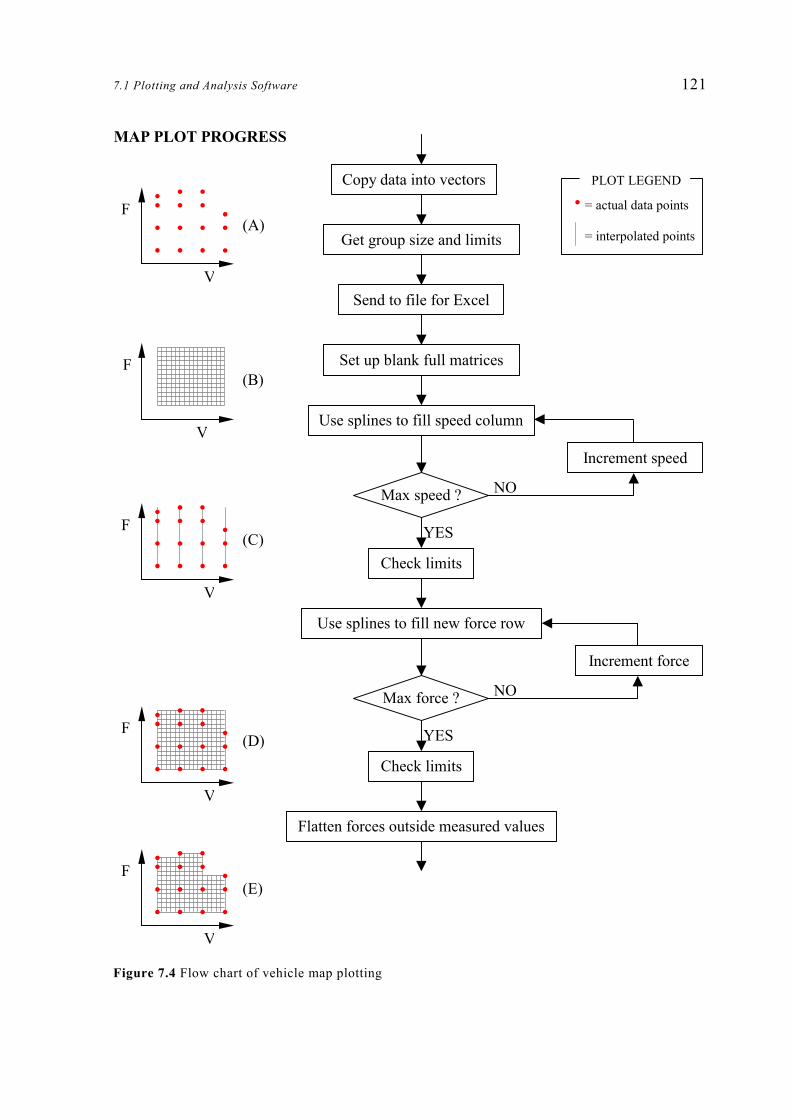
7.1 Plotting and Analysis Software 121
Figure 7.4 Flow chart of vehicle map plotting
Get group size and limits
Send to file for Excel
Set up blank full matrices
NO
YES
Copy data into vectors
Use splines to fill speed column
Max speed ?
Increment speed
Check limits
Use splines to fill new force row
Increment force
NO
YES
Max force ?
Check limits
Flatten forces outside measured values
F
F
F
F
V
V
V
V
F
V
MAP PLOT PROGRESS
= actual data points = interpolated points (A)
(E)
(D)
(C)
(B)
PLOT LEGEND

122 CHAPTER 7: Data Analysis and Presentation Software
speed columns but the maximal number of rows. The user can adjust the level of
interpolation to achieve a smoother plot, and does so by setting the maximum number
of data points to be interpolated on the x- and y-axes. A greater number of points
takes more time to calculate, but provides a better looking and more accurate
representation. The second matrix has the full number of rows and columns (B), and
it is this matrix that is plotted using the MATLAB command surf. Each column of
the intermediate matrix is filled out using columns from the original data and the
MATLAB spline command. This function uses cubic splines to replicate the data
at each original point, and interpolate for the points in between. Figure 7.5 shows a
cubic spline interpolation, which extends a seven point series to a 101 point series,
with a greater upper limit. This process places the full number of load rows into each
speed column of the first intermediate matrix (C).
0 200 400 600 800 1000 1200 1400 160010
15
20
25
Tractive Force (N)
z- p
aram
eter
(e.g
. Effi
cien
cy)
Original data pointsInterpolated points
Figure 7.5 Example of cubic spline interpolation
When each of the original speeds has been traversed in this way, each z-value (i.e.
the ‘heights’ of the graph) is checked against user-defined limits. Usually, a
minimum of zero ensures that the spline function does not dip too low between data
points, and a maximum can also be set for specialised plotting applications. If any of
the spline values lie outside the allowable range, they are made equal to the limit. For
example, if the lower limit was set at 10 and one of the interpolated z-values became
9.7, the checking routine would simply substitute a 10 in place of the 9.7.
Next, the intermediate matrix is used to fill the full plotting matrix by implementing
spline functions along each of the new rows. In this case, each of the rows will be the
same length—as each set of loads was conducted at similar speeds—and each is

7.1 Plotting and Analysis Software 123
interpolated to pad it out to the maximal number of points. At this stage, the second
matrix (containing all the interpolated z-values) could be plotted using the surf
function with appropriate x and y vectors (D). However, the filled out matrix includes
full speed columns containing tractive effort points exceeding those that the test
vehicle was able to produce. After the limits are again checked, all the matrix values
that lie outside the original data range are set to zero—or some other user-defined
value (E). Thus, an abrupt change in ‘height’ is encountered in the final plot to
indicate the end of the measured data. When viewing in three-dimensional mode, this
flattened area appears as such and can be misleading to the uninitiated observer. The
option to whiteout the zeroed area is also made available to the user, and is
particularly effective when viewing data solely as a colour contour plot from above.
2-D and 3-D plots are shown in Figures 7.6 and 7.7 for the same fuel flowrate data
from the test vehicle.
7.1.3.3 Microsoft Excel Display
As well as providing a graphical display, it is useful to be able to view vehicle
mapping data in its raw form. The recorded data may be viewed directly in the text
file to which it was saved, or in a pseudo-graphical layout that sets out the
information in tabular form. Microsoft Excel has been used to develop a format that
displays the measured parameters in a grid that lines up with the speed and load at
which each point was recorded. An example is shown in Figure 7.8, which represents
the same mapping run as that shown in Figures 7.6 and 7.7.
Because the Excel grid is discrete, approximations must be made to assign the
measured data points to one cell only. At each set-speed, the tractive force points will
each be recorded at a slightly different velocity—despite the power absorber
controlling in speed mode. To avoid the need for infinite horizontal variation within
the columns, the average measured velocity at each set-speed has been substituted as
an approximation for all the speeds in that column (e.g. all the data points recorded at
a nominal velocity of 100 kph). On the vertical axis, the tractive force recorded at
each data point has been rounded to the nearest 25 N step. For example, the data
points in cells level with the 800 N label are known to lie in the range 787.5–812.5
(i.e. 800±12.5 N). Figure 7.8 shows a point just above the 800 N line at a velocity of

124 CHAPTER 7: Data Analysis and Presentation Software
39 kph. This point was recorded with the measured tractive effort between 812.5 and
837.5 (or 825±12.5 N).
Figure 7.6 Two dimensional contour mapping plot for Toyota Celica fuel flowrate
Figure 7.7 Three dimensional contour mapping plot for Toyota Celica fuel flowrate
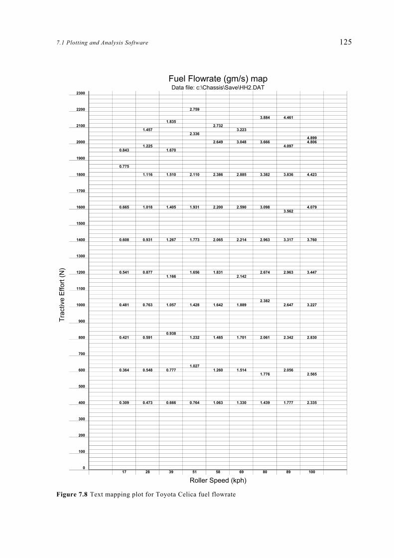
7.1 Plotting and Analysis Software 125
Figure 7.8 Text mapping plot for Toyota Celica fuel flowrate
Fuel Flowrate (gm/s) mapData file: c:\Chassis\Save\HH2.DAT
2300
2200 2.759 3.884 4.461 1.835
2100 2.732 1.457 3.223 2.336 4.899
2000 2.649 3.048 3.666 4.806 1.225 4.097 0.843 1.670
1900 0.775
1800 1.116 1.510 2.110 2.386 2.885 3.382 3.836 4.423
1700
1600 0.665 1.018 1.405 1.931 2.200 2.590 3.098 4.079 3.562
1500
1400 0.608 0.931 1.267 1.773 2.065 2.214 2.963 3.317 3.760
1300
1200 0.541 0.877 1.656 1.831 2.674 2.963 3.447 1.166 2.142
1100 2.382
1000 0.481 0.763 1.057 1.428 1.642 1.889 2.647 3.227
900 0.938
800 0.421 0.591 1.232 1.485 1.701 2.061 2.342 2.830
700 1.027
600 0.364 0.548 0.777 1.260 1.514 2.056 1.776 2.565
500
400 0.309 0.473 0.666 0.764 1.063 1.330 1.439 1.777 2.335
300
200
100
0 17 28 39 51 58 69 80 89 100
Roller Speed (kph)
Trac
tive
Effo
rt (N
)

126 CHAPTER 7: Data Analysis and Presentation Software
In practice, these text plots are produced using an Excel macro (included in the
template spreadsheet on CD), which performs the function of copying the data from a
predefined file and transferring it into the plot area. To produce a plot such as Figure
7.8, the user must first generate a mapping plot in the MATLAB post-processing
program, then the standard plot sheet is opened in Excel and the macro can be run.
As part of the MATLAB plotting routine, a new text file is set up, which lays out the
mapping data in a form that is easily copied into Microsoft Excel. This file consists
of a regular grid, with zeros taking the place of load/speed combinations for which
there is no recorded data. Another text file is also generated, which consists solely of
a list of the three parameters for that map (speed, tractive force, and fuel flowrate, for
example). This file is useful for comparisons between runs where the variations (e.g.
in maximum tractive effort) may only be very small, and would not be visible on
either the Excel text plot or the contour plots. Examples of the text file and the
standard Excel plot sheet are included in Appendix X. The spreadsheet file also
contains the average speeds for labelling the columns, and information such as the
name and units of the variable to be displayed.
7.1.4 Driving Cycle Error Analysis
During driving cycle tests, adherence to the prescribed speed demand is measured in
terms of a speed and time tolerance. Limits of ±1 kph in speed and ±0.5 seconds in
time were chosen for the testing detailed in Chapter 8. This driving cycle tolerance is
shown graphically in Appendix V. Although the C++ data acquisition routine
calculates the excursions during the driving cycle run (see Section 6.5.12.1) it is
useful to be able to apply different tolerances (to comply with different testing
standards) after the test has been carried out.
The calculation of driving cycle excursions is included as an option in the ‘Calculate
Additional Data’ menu of the MATLAB program and is conducted in a similar way
to that used in the C++ testing control routine. The user is first prompted for the
desired velocity (kph) and time (sec) tolerances, the latter of which is converted to a
number of time steps (e.g. 0.8 seconds = 8 time steps at 10 Hz). The driving cycle
sequence is then traversed one data point at a time, comparing the measured velocity
at the present time to the cycle target speed within the limits. Figure 7.9 shows two

7.1 Plotting and Analysis Software 127
separate points being investigated and compared against the velocity range of all the
demand speeds within the time envelope. In the example, the time and speed
tolerances are 0.5 sec and 1 kph respectively. At each point, the time envelope
consists of desired speeds 0.5 sec (five points) either side of the present time. To
remain within the limits, the current measured speed must be less than the maximum
cycle speed in the time envelope plus the speed allowance (1 kph), and greater than
the minimum cycle speed in the envelope minus the speed allowance.
Example A
Cycle velocities included in time envelope = 0, 0, 0, 0, 0, 0.1, 0.2, 0.3, 0.4, 0.5, 0.6
Maximum cycle velocity in time envelope = 0.6 kph Maximum allowable vehicle speed = 0.6 + tolerance = 0.6 +1.0 = 1.6 kph
Minimum cycle velocity in time envelope = 0.0 kph Minimum allowable vehicle speed = 0.0 - tolerance = 0.0 – 1.0 = –1.0 kph
Current speed = 0.0 kph
∴ Since –1.0 ≤ 0.0 ≤ 1.6 the current speed is within the allowable limits
Example B
Cycle velocities included in time envelope = 5, 5, 5, 4.5, 4, 3.5, 5, 2.5, 2, 1.5, 1
Maximum cycle velocity in time envelope = 5.0 kph Maximum allowable vehicle speed = 5.0 + tolerance = 5.0 +1.0 = 6.0 kph
Minimum cycle velocity in time envelope = 1.0 kph Minimum allowable vehicle speed = 1.0 - tolerance = 1.0 – 1.0 = 0.0 kph
Current speed = 6.4 kph
∴ Since 0.0 ≤ 6.4 < 6.0 the current speed is not within the allowable limits
Figure 7.9 Examples of velocity and time compliance calculation
The total excursion time (time spent outside the allowable limits) is displayed after
this process is completed, and the cumulative excursion time is also stored as part of
Time -0.5s Current +0.5stime
Cycle (kph) 0 0 0 0 0 0.1 0.2 0.3 0.4 0.5 0.6Measured (kph) 0 0 0 0 0 0 0 0 0.4 1.0 1.1
Time -0.5s Current +0.5stime
Cycle (kph) 5 5 5 4.5 4 3.5 3 2.5 2 1.5 1Measured (kph) 5 5.5 6.5 6.4 6.4 6.4 6 5 3.5 2.0 1

128 CHAPTER 7: Data Analysis and Presentation Software
the large data matrix so that it may be plotted against time, or any other driving cycle
parameter.
7.2 Vehicle Energy Consumption Modelling
During a driving cycle, the vehicle under test consumes energy from its fuel source
(be it electrical or chemical) and puts out power at the road wheels. It is important to
be able to model the amount of energy used during a period of driving, so that the
relative effects of friction, gravitational, and inertial forces can be investigated. The
vehicle energy consumption modelling program is a simple, stand alone MATLAB
routine than can be used to calculate either the total energy output of a vehicle under
test, or the total energy that should be required by a vehicle undergoing a certain
driving cycle. The ideal energy consumption for a given vehicle can be compared
with the actual measured result to determine the effectiveness of the driving cycle
routine and dynamometer road load demand functions.
Both the ideal-cycle and the measured-output functions make use of text files with a
single column of numerical data. For calculating the predicted cycle output, the input
file must contain a sequence of desired cycle speeds. The user must also provide
vehicle details such as the mass and frictional coefficients so that the tractive force
(and hence power) required to achieve a given acceleration and velocity can be
calculated using Equation 7-3. The optional gravitational term, mV gsinθ may be
included if the effect of road gradient is to be modelled. For calculating the actual
vehicle energy output during a test, power measurements—corrected for atmospheric
conditions—are required. Also necessary for both processes is the idle power
consumption of the vehicle. Idle power represents the minimum amount of power that
an engine will put out, and is discussed in more detail in Section 7.2.1.
2210 vfvffgm
dtdvmF VVVVVeqV ++++= θsin (7-3)
( ) vFduncorrecteOutputPower V .= (7-4)
For the purpose of modelling the vehicle forces in Equation 7-3, the acceleration is
calculated from the desired driving cycle speeds using a central difference

7.2 Vehicle Energy Consumption Modelling 129
approximation (see Equation 7-1). The power at each given velocity point is
corrected for the atmospheric temperature and pressure (as per Equation 6-5), then
multiplied by the time interval over which it is assumed to have been maintained,
giving the energy consumed. The sum of each of these energy steps yields the total
energy consumed over the entire driving cycle.
( ) tPJConsumedEnergy corr∆Σ= (7-5)
Where: t∆ = length of each time interval between readings (sec)
The calculation of the measured power uses the corrected power values as returned
by the C++ control program. Equation 7-5 is again used to generate the total energy
consumed over the entire run.
7.2.1 Vehicle Idle Power
Equation 7-5 may be used to calculate the total energy consumed over a driving cycle
in the ideal and real-world cases. However, there are times when the output power
used in this equation becomes less than is practical for the engine to deliver,
particularly when testing with internal combustion engines. When the vehicle engine
is idling (i.e. velocity = 0), and especially during decelerations (mVeq dv/dt < 0) the
power output may be zero or negative. Unless the test vehicle employs regenerative
braking, this zero or negative energy output value is not possible, and some
assumption must be made. Thus, we employ what is known as an idle power, and
assume for the purposes of energy consumption calculations that the power output
cannot drop below this value. From the point of view of the fuel energy, there is a
certain level of consumption that the internal combustion engine requires to
overcome its internal friction and continue running when no throttle is applied. Since
no throttle is applied during stationary or braking periods, it is logical to substitute
the idle power under these circumstances.
If PowerIdlePower <
Assume PowerIdlePower =

130 CHAPTER 7: Data Analysis and Presentation Software
As for the actual idle power magnitude, there are several approaches that may be
applied. Vehicle energy consumption modelling previously carried out at the
University of Canterbury [Epps, 1987] approximated the idle power as the power
generated under slow driving conditions. Specifically, the idle power was calculated
as the road load force at 10 kph multiplied by this velocity. An experimental method
was desired to verify the suitability of this approximation, using measured power
output and fuel consumption. Because power output can only be measured by the
chassis dynamometer in terms of force and speed at the drums, a relationship was
sought between idle power and the output power when a vehicle is driving on the
dynamometer. Assuming that the engine efficiencies are similar during idle and low
speed driving, the following equation will be true:
runningduringPower
idleduringPowerrunningduringnconsumptioFuel
idleduringnconsumptioFuel= (7-6)
To ensure that the driving conditions were as similar as possible to idle, the vehicle
was driven in low gear with the engine running at the idle speed. With modern
vehicles employing automatic choke, a state is easily achieved wherein the vehicle is
propelled at a constant speed with no application of the accelerator pedal. For the test
vehicle discussed in Chapter 8, idle speed and no-throttle motion were both achieved
at an engine speed of approximately 650 rpm. At this point, the engine is supplying
enough power to continue running (idle power) plus an additional power output to
overcome rolling resistances and the chassis dynamometer friction. We assume that
vehicle resistances are small and that the dynamometer friction (measured as tractive
effort at the drums) represents the majority of the power consumption over and above
the idle. Since fuel consumption during idle and driving can both be measured—
along with the tractive effort and speed—idle power remains the only unknown in
Equation 7-6. The test vehicle is used as an example in the calculation of idle power:
Fuel consumption at idle (650 rpm) = 0.167 gm/s
Fuel consumption while running (650 rpm) = 0.183 gm/s
Power generated at drums during idling = 0 W
Power generated at drums while running = 110 W
7.2 Vehicle Energy Consumption Modelling 131
913.0183.0167.0
==runningduringnconsumptioFuel
idleduringnconsumptioFuel
Idling takes up 91.3% of the fuel (i.e. turning the dynamometer takes up 8.7%)
Power consumed by the dynamometer during running = 110W = 8.7% of total
Total power consumed = 11078
100×
. = 1264W
Idle Power = 1264 – 110 = 1154 W
This is significantly greater than the 600 W calculated using the vehicle road load at
10 kph. If the fuel consumption that is applied to the unmeasured transmission and
rolling friction components could be measured and accounted for, the resulting
experimental value would be closer to the approximation used by Epps. Considering
that the idle power magnitudes in question were not great in comparison to the
overall vehicle outputs, the experimental value was rounded down, and an idle power
of 1000 W was implemented for the results quoted in Chapter 8.


CHAPTER 8:
Vehicle Testing Procedure and Sample Results
8.1 The Test Vehicle
The vehicle tests discussed in this chapter were carried out on a 1982 Toyota Celica
owned by the University of Canterbury. This rear-wheel drive car was powered by a
6 cylinder, fuel injected, 2 litre engine and had completed approximately 206 000 km
before testing commenced. Further details are included in the Vehicle Data Sheet (see
Appendix Y), which is to be filled out for all vehicles tested on the chassis
dynamometer. This section contains information regarding the on-road friction
determination, and specific details of the dynamometer set up for the Toyota Celica,
hereafter referred to as the test vehicle.
Plate 8.1 The test vehicle

134 CHAPTER 8: Vehicle Testing Procedure and Sample Results
8.1.1 Vehicle Friction Determination
In order to carry out realistic road load modelling on the chassis dynamometer, the
frictional forces acting on the test vehicle during on-road driving must be determined
or estimated. Deceleration tests have been used with considerable success in the past
([White & Korst, 1972], [Hindin, 1985]) and a method for conducting these
coastdowns is described in detail in SAE J1263 [1999]. With knowledge of the
vehicle mass, the frictional forces can be calculated from acceleration and velocity
measurements between two given speeds. In practice, several on-road decelerations
were performed and the results averaged.
The vehicle speed was measured and recorded electronically during each run by a
purpose-built optical pickup mounted on the underside of the vehicle. A white strip
was painted on the driveshaft, allowing each revolution to be detected and timed.
Before the coastdowns were carried out, the number of driveshaft revolutions per
wheel rotation was calculated by rolling the vehicle forward a set number of
rotations, and measuring the distance. Although this method does not take into
account possible changes in tyre diameter at high speed, it was thought to be
sufficiently accurate when the vehicle tyres were inflated to recommended pressures.
By keeping a record of the number of 2 µs time intervals between consecutive
driveshaft rotations, the instantaneous velocity could be calculated (see Equations 8-1
and 8-2). An example resulting velocity coastdown curve is given in Figure 8.1.
( )×= pulseclockperTimerotationdriveshaftperTime
( )rotationperpulsesclockofNumber (8-1)
rotationdriveshaftperTime
rotationdriveshaftperDistanceVelocity = (8-2)
As well as vehicle mass, the calculation of friction constants requires information
regarding air temperature and pressure during coastdowns, and the frontal area of the
vehicle. The latter can be determined using an elevational photograph as shown in
Appendix Z. The SAE procedure allows for wind conditions and small road
gradients, among other factors, and the full calculation of vehicle friction is also
included in Appendix Z.

8.1 The Test Vehicle 135
0 10 20 30 40 50 6030
40
50
60
70
80
90
100
110
120
Time (sec)
Veh
icle
vel
ocity
(kph
)
Figure 8.1 Coastdown velocity vs. time curve
The total on-road vehicle friction was found to be:
2413043909214 vvFV ... +−= (8-3)
With: v = velocity in m/s
These coefficients were used to calculate the net power absorber force required for
road load simulation of the test vehicle on the dynamometer according to Equation 3-
10. Theoretically, each of these constants should be positive, so that the friction
always increases with velocity. However, the linear velocity coefficient (f1V) shown
above was calculated as a negative value, which was most likely a result of the least
squares approximation. Vehicle coastdown data may be prone to this type of error, as
the least squares curve fit is required to extrapolate beyond the minimum measured
speed of 40 kph.
The f0Vd, f1Vd, and f2Vd coefficients in Equation 3-10 were determined in a series of
coastdowns with the test vehicle on the chassis dynamometer. The curb weight of the
test vehicle was given as 1150 kg [Coomber, 1988], to which 100 kg was added to
account for driver and fuel weight. In general, each vehicle should be accurately

136 CHAPTER 8: Vehicle Testing Procedure and Sample Results
weighed before testing. The standard approximation for the vehicle’s inertial mass
(see Section 3.1) resulted in an equivalent vehicle mass of 1290 kg. An equivalent
flywheel mass of 1234 kg was employed for all subsequent tests, requiring that the
eddy-current dynamometer output be as follows for the appropriate road load
simulation:
( ) ( ) ( ) ( ) 222110012341290 vffvffff
dtdvF VdVVdVVdVpa −+−+−+−= (8-4)
With: f0V etc. from latest friction calibration
8.1.2 Specifics of Test Vehicle Set Up
Before testing, any vehicle must be tied down on the dynamometer rollers and have
the appropriate instrumentation attached. For the Toyota Celica, the rear wheels were
kept in contact with the roller drums using steel cables and turnbuckles provided for
this purpose in the chassis dynamometer laboratory. The front wheels could be
chocked, but it was found that the cabling alone was sufficient for lateral and
longitudinal stability.
The test vehicle oil level indicator was removed, and the engine oil temperature was
monitored by means of a thermocouple mounted in a substitute dipstick. Vehicle
cooling water temperature was measured using a thermocouple inserted in the cooling
circuit at the entrance to the radiator.
To measure the air-flow into the engine, the factory air filter intake was removed,
and the Annubar drum output taped in its place. The seals and drain-holes in the filter
were then plugged with RTV rubber compound so that all air entering the engine was
required to pass through the flow measurement device. Air flowrates for the test
vehicle were in the range 0–70 gm/s, requiring the larger of the two Annubar tubes to
be used throughout the testing detailed in this chapter (see Appendix C.7 for Annubar
description and calibration).
Measuring the fuel flowrate through the test vehicle’s fuel injection system with a
single flowmeter required some additional fuel line equipment. In most fuel injection
systems, fuel is supplied to the injector rail at high pressure, and any excess that is

8.2 Sample Test Results 137
not used in the cylinders is returned to the tank via a separate line. By blocking the
return line and re-routing the fuel as shown in Appendix C.6, all the fuel was made to
pass through the Fluidyne flowmeter, enabling a single consumption value to be
recorded. Plate 8.2 below shows the test set up viewed from the front of the vehicle.
Plate 8.2 Test vehicle engine instrumentation
8.2 Sample Test Results
The test results discussed in this section were gathered in a series of trials conducted
during November and December 2001, and January 2002. Several initial tests (not
included here) were conducted to enable debugging and familiarisation with the
equipment and vehicle driving techniques. All test data relates to the Toyota Celica
test vehicle running on 96 octane petrol.
8.2.1 Test Vehicle Warm Up
Before each test session, both the chassis dynamometer and test vehicle were
thoroughly warmed up. This generally began with of a period of time running under
power from the electric motor with the vehicle engine idling and gearbox in neutral.
Progressively faster roller speeds were introduced, while monitoring the drum axle
oil temperature. After approximately 15 minutes of running, and with an axle oil
FUEL FLOWMETERAIR INTAKE
FROM ANNUBARSYSTEM
ENGINE OIL AND WATER TEMPERATURE
THERMOCOUPLE LEADS

138 CHAPTER 8: Vehicle Testing Procedure and Sample Results
temperature of at least 47º (assisted by the oil heater) a brief period of high speed
running (>100 kph for approximately 2 minutes) was conducted before the vehicle
transmission was engaged. Switching off the electric motor and driving the
dynamometer under power from the vehicle, the engine, tyres, and transmission were
then warmed up. Speeds were varied and a moderate rate of engine revving
(2000–3000 rpm) employed until the engine oil and cooling water both approached
operating temperatures (>80º). Part of this vehicle warm up was often accomplished
by following a driving cycle, particularly as practice for the driver before a recorded
driving cycle test.
8.2.2 Maximum Throttle Acceleration Curves
Maximum throttle accelerations were carried out on the test vehicle mostly in 2nd
gear and with no power absorber load. Slower accelerations brought about by the
addition of dynamometer load or the use of higher gears did not significantly affect
the underlying trends. As detailed in Section 6.5.9, the ‘Manual Control’ mode was
used to facilitate these accelerations, during which recording generally began at
about 35 kph and ceased at 5500–6000 rpm. Figure 8.2 shows three separate
maximum throttle accelerations, one of which includes a power absorber load of 100
Nm. These graphs were plotted using the MATLAB filtering and power calculation
routine discussed in Section 7.1.3.1.
The average maximum power for these three runs was 53.2 kW at 4800 rpm, with a
standard deviation of 0.5 kW (1.0%). The highest peak reading was achieved during
the run involving significant dynamometer load. This added load has the effect of
slowing the acceleration and allowing the engine more time to stabilise the power
output, resulting in a greater power. Although exact model information for the test
vehicle could not be found, other Toyotas manufactured in 1982 and with comparable
engines were listed by Autodata [1990] with a peak output power of around 90 kW.
Manufacturers’ power ratings are most often quoted in terms of engine output, so the
driveline and peripheral equipment (e.g. fan-belt) losses are not included. An
estimate of engine power at the flywheel may be arrived at by adding the
transmission and rolling resistances (measured by coastdown on the dynamometer) to

8.2 Sample Test Results 139
the measured tractive effort. Peak power at the flywheel calculated in this way was
slightly higher, at 54.7 kW.
2000 2500 3000 3500 4000 4500 5000 5500 600020
25
30
35
40
45
50
55
Engine RPM (rpm)
Pow
er (
kW)
Figure 8.2 Power curves for test vehicle (green curve includes 100 Nm dynamometer load)
The average output power of 53 kW at the road surface was lower than expected, but
was thought to be realistic in light of the inevitable decrease in peak power brought
about by general wear and tear on the test vehicle.
The relationship between maximum engine torque (directly related to tractive force)
and speed can also be investigated using full throttle accelerations. With the
corrected tractive effort measurements used to calculate power in the previous
paragraph, similar graphs can be plotted using the chassis dynamometer MATLAB
routines.
It can be seen that the torque is more evenly distributed throughout the engine speed
range than power, and has a less predictable form. Peak tractive effort (measured at
the roller drums) from the same three acceleration runs as above was found to be
2880 N on average, with a standard deviation of 40 N (1.4%). The maximum tractive
force was recorded at an engine speed of 4000 rpm (to the nearest 50 rpm).

140 CHAPTER 8: Vehicle Testing Procedure and Sample Results
2000 2500 3000 3500 4000 4500 5000 5500 60001600
1800
2000
2200
2400
2600
2800
3000
Engine RPM (rpm)
Trac
tive
For
ce (
N)
Figure 8.3 Tractive force curves for test vehicle (green curve includes 100 Nm dynamometer load)
8.2.3 Vehicle Mapping Tests
Several vehicle mapping tests were carried out in 3rd gear according to the method
described in Section 6.5.11. With the driver setting the throttle for tractive effort, and
the power absorber in speed-control mode, each tractive force up to the vehicle’s
limit was recorded at each set speed. Each complete mapping test run took 30–45
minutes to complete, depending on how rapidly the desired loads were achieved and
whether or not the emissions equipment was in use.
8.2.3.1 Mapping Plot Form
Figure 8.4 shows two separate mapping tests, displaying the results in graphical form
using the MATLAB plotting package described in Chapter 7. For all the vehicle maps
shown in this chapter, vehicle speed is plotted on the x-axis, with tractive force on
the y-axis. The map parameter of interest is displayed in the z-direction as colour
contours, height and colour (see Figure 7.7) or plain text (see Figure 8.5).
The uneven shape observed at the top of each graph in Figure 8.4 is a result of the
maximum force output at each given speed, which occurs when full throttle is
z
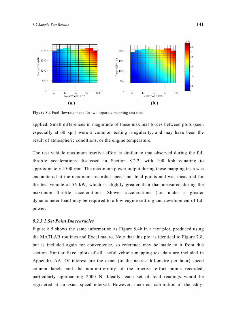
8.2 Sample Test Results 141
(a.) (b.)
Figure 8.4 Fuel flowrate maps for two separate mapping test runs.
applied. Small differences in magnitude of these maximal forces between plots (seen
especially at 60 kph) were a common testing irregularity, and may have been the
result of atmospheric conditions, or the engine temperature.
The test vehicle maximum tractive effort is similar to that observed during the full
throttle accelerations discussed in Section 8.2.2, with 100 kph equating to
approximately 4500 rpm. The maximum power output during these mapping tests was
encountered at the maximum recorded speed and load points and was measured for
the test vehicle at 56 kW, which is slightly greater than that measured during the
maximum throttle accelerations. Slower accelerations (i.e. under a greater
dynamometer load) may be required to allow engine settling and development of full
power.
8.2.3.2 Set Point Inaccuracies
Figure 8.5 shows the same information as Figure 8.4b in a text plot, produced using
the MATLAB routines and Excel macro. Note that this plot is identical to Figure 7.8,
but is included again for convenience, so reference may be made to it from this
section. Similar Excel plots of all useful vehicle mapping test data are included in
Appendix AA. Of interest are the exact (to the nearest kilometre per hour) speed
column labels and the non-uniformity of the tractive effort points recorded,
particularly approaching 2000 N. Ideally, each set of load readings would be
registered at an exact speed interval. However, incorrect calibration of the eddy-
z

142 CHAPTER 8: Vehicle Testing Procedure and Sample Results
Figure 8.5 Fuel flowrate text map for test vehicle (duplicates Figure 7.8)
Fuel Flowrate (gm/s) mapData file: c:\Chassis\Save\HH2.DAT
2300
2200 2.759 3.884 4.461 1.835
2100 2.732 1.457 3.223 2.336 4.899
2000 2.649 3.048 3.666 4.806 1.225 4.097 0.843 1.670
1900 0.775
1800 1.116 1.510 2.110 2.386 2.885 3.382 3.836 4.423
1700
1600 0.665 1.018 1.405 1.931 2.200 2.590 3.098 4.079 3.562
1500
1400 0.608 0.931 1.267 1.773 2.065 2.214 2.963 3.317 3.760
1300
1200 0.541 0.877 1.656 1.831 2.674 2.963 3.447 1.166 2.142
1100 2.382
1000 0.481 0.763 1.057 1.428 1.642 1.889 2.647 3.227
900 0.938
800 0.421 0.591 1.232 1.485 1.701 2.061 2.342 2.830
700 1.027
600 0.364 0.548 0.777 1.260 1.514 2.056 1.776 2.565
500
400 0.309 0.473 0.666 0.764 1.063 1.330 1.439 1.777 2.335
300
200
100
0 17 28 39 51 58 69 80 89 100
Roller Speed (kph)
Trac
tive
Effo
rt (N
)
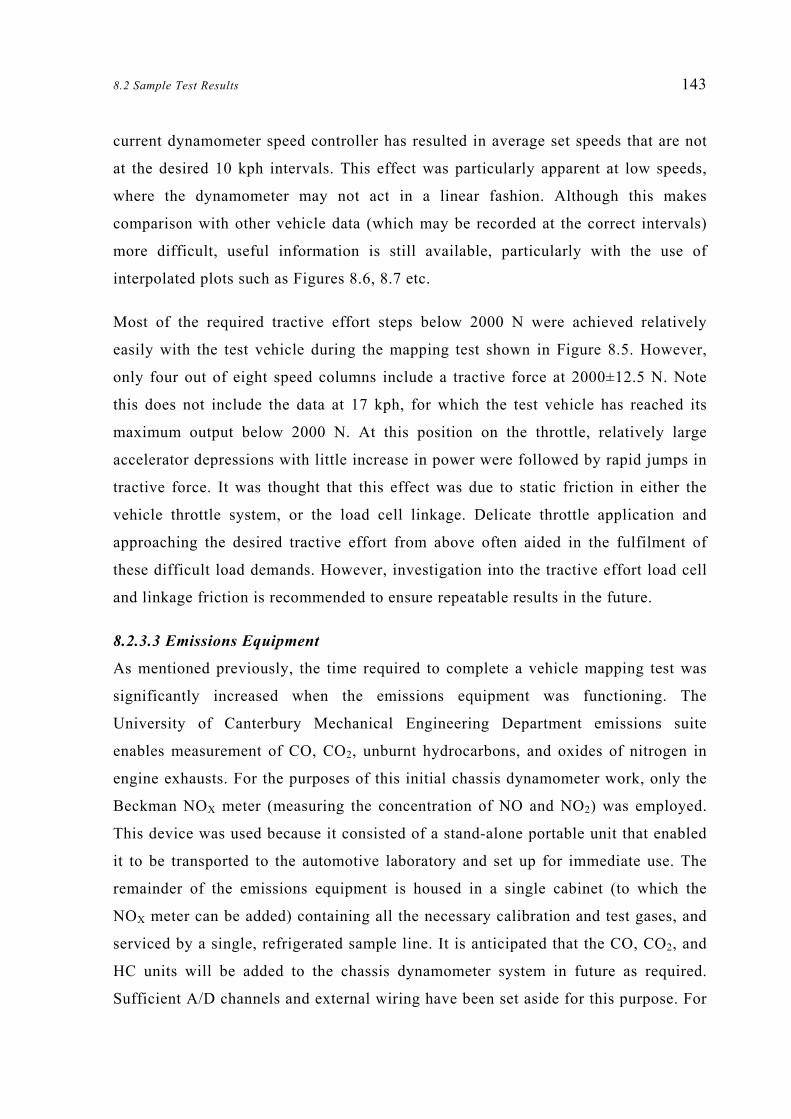
8.2 Sample Test Results 143
current dynamometer speed controller has resulted in average set speeds that are not
at the desired 10 kph intervals. This effect was particularly apparent at low speeds,
where the dynamometer may not act in a linear fashion. Although this makes
comparison with other vehicle data (which may be recorded at the correct intervals)
more difficult, useful information is still available, particularly with the use of
interpolated plots such as Figures 8.6, 8.7 etc.
Most of the required tractive effort steps below 2000 N were achieved relatively
easily with the test vehicle during the mapping test shown in Figure 8.5. However,
only four out of eight speed columns include a tractive force at 2000±12.5 N. Note
this does not include the data at 17 kph, for which the test vehicle has reached its
maximum output below 2000 N. At this position on the throttle, relatively large
accelerator depressions with little increase in power were followed by rapid jumps in
tractive force. It was thought that this effect was due to static friction in either the
vehicle throttle system, or the load cell linkage. Delicate throttle application and
approaching the desired tractive effort from above often aided in the fulfilment of
these difficult load demands. However, investigation into the tractive effort load cell
and linkage friction is recommended to ensure repeatable results in the future.
8.2.3.3 Emissions Equipment
As mentioned previously, the time required to complete a vehicle mapping test was
significantly increased when the emissions equipment was functioning. The
University of Canterbury Mechanical Engineering Department emissions suite
enables measurement of CO, CO2, unburnt hydrocarbons, and oxides of nitrogen in
engine exhausts. For the purposes of this initial chassis dynamometer work, only the
Beckman NOX meter (measuring the concentration of NO and NO2) was employed.
This device was used because it consisted of a stand-alone portable unit that enabled
it to be transported to the automotive laboratory and set up for immediate use. The
remainder of the emissions equipment is housed in a single cabinet (to which the
NOX meter can be added) containing all the necessary calibration and test gases, and
serviced by a single, refrigerated sample line. It is anticipated that the CO, CO2, and
HC units will be added to the chassis dynamometer system in future as required.
Sufficient A/D channels and external wiring have been set aside for this purpose. For

144 CHAPTER 8: Vehicle Testing Procedure and Sample Results
the vehicle testing discussed in this chapter, the NOX meter was supplied by a 4 m
section of Teflon tubing with two condensate traps. During changes in engine output,
delays of approximately 10 seconds were encountered as the sample exhaust gas
travelled down the supply line, through the NOX meter sample refrigerator, and into
the reaction chamber. It was decided that mapping test points should be held by the
driver for at least 12 seconds each to ensure sample stability whenever NOX
emissions were to be tested.
As well as the necessary delays at each map point, additional difficulties were
encountered during testing with the Beckman NOX meter. The results from several
mapping tests showed that the NOX concentration measurements gathered in this way
were highly variable and perhaps affected by the sample temperature and state of the
system pump. For three such mapping tests, the average standard deviation between
comparable values from each run was 165 ppm, or 5.9% of the maximum value. That
is, if a large number of mapping tests were conducted, 95% of values would be
expected to lie within 165 parts per million of the average for that set point. Later
tests showed progressively worse repeatability as the pump began to overheat. It was
expected that the sample pressure became insufficient under these conditions, and the
condition of the NOX meter pump should be investigated before any further emissions
testing is carried out. To ensure a dry exhaust sample, one moisture trap was
positioned close to the tailpipe, and a second was included in the NOX meter flow
circuit prior to entry into the reaction chamber. These devices incorporated
containers of ice to facilitate condensation, which needed to be refilled during the
course of a mapping test. Fresh ice was added—and any condensate removed—at two
separate instances, usually between the speeds of 80 and 70 kph, as well as between
the 50 and 40 kph data groups (note that the speeds were recorded in descending
order). This process will not be necessary once when the entire emissions suite is in
use with the accompanying refrigerated sample line. Figure 8.6 shows an example
map plot with NOX concentrations represented by colour contours.
The concentration of nitrogen oxides in the exhaust gas was greatest when the vehicle
was under maximum power conditions, and peaks of approximately 2700 ppm can be
z

8.2 Sample Test Results 145
Figure 8.6 NOX concentration map for test vehicle
seen in the upper right hand corner of Figure 8.6. There is also a secondary area of
higher NOX concentration at speeds near 50 kph with tractive forces above 1200 N.
8.2.3.4 Selected Results
As well as the exhaust emissions, several other useful parameters were measured or
calculated from mapping runs on the test vehicle. Fuel consumption is particularly
important, and may be expressed in terms of miles per gallon, litres per 100 km, or
kilometres per litre (the latter of which is shown in Figure 8.8). Energy consumption,
efficiency, and air-fuel ratio also depend on the measured fuel flowrate. Table 8.1
contains a summary of the variation in data at each measured point, combining three
separate vehicle mapping tests. Standard deviations are given in their respective
units, and as a percentage of the maximum measured value. That is, where an
identical load (±12.5 N) and speed point (±1 kph) were present in each of the three
runs, the three z-values were combined to record a standard deviation (which was
then averaged with all the other matching points). Where the load and speed points
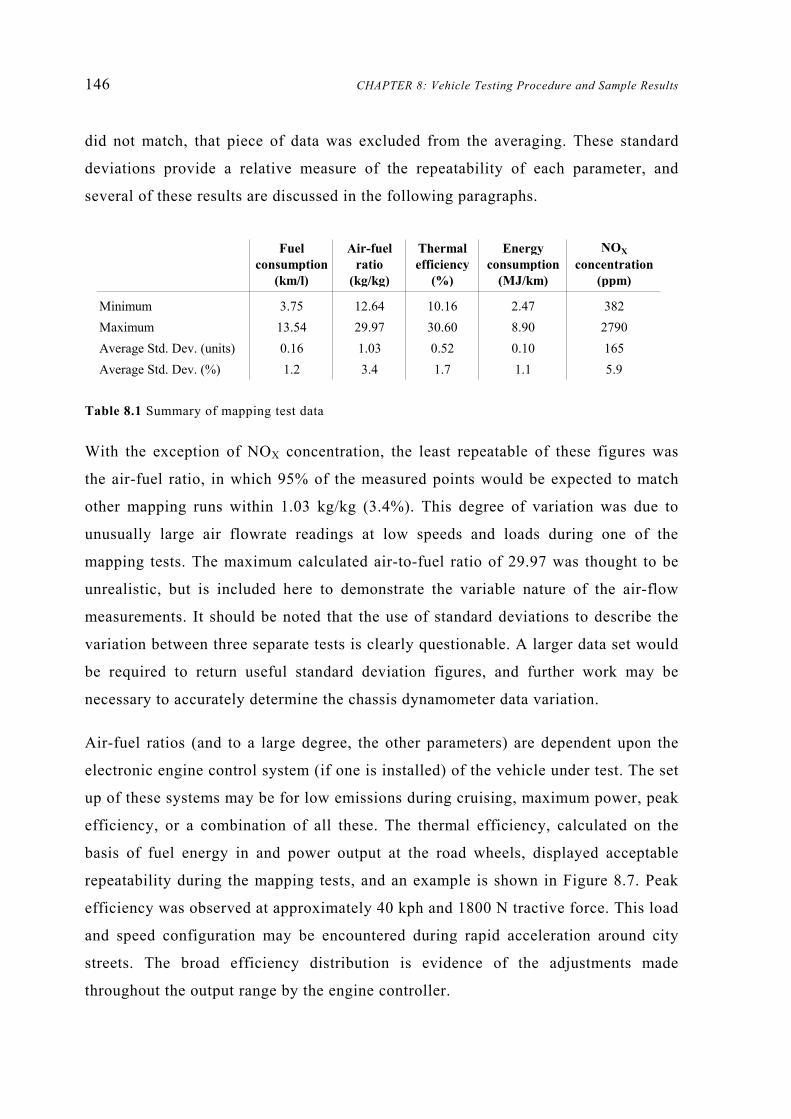
146 CHAPTER 8: Vehicle Testing Procedure and Sample Results
did not match, that piece of data was excluded from the averaging. These standard
deviations provide a relative measure of the repeatability of each parameter, and
several of these results are discussed in the following paragraphs.
Table 8.1 Summary of mapping test data
With the exception of NOX concentration, the least repeatable of these figures was
the air-fuel ratio, in which 95% of the measured points would be expected to match
other mapping runs within 1.03 kg/kg (3.4%). This degree of variation was due to
unusually large air flowrate readings at low speeds and loads during one of the
mapping tests. The maximum calculated air-to-fuel ratio of 29.97 was thought to be
unrealistic, but is included here to demonstrate the variable nature of the air-flow
measurements. It should be noted that the use of standard deviations to describe the
variation between three separate tests is clearly questionable. A larger data set would
be required to return useful standard deviation figures, and further work may be
necessary to accurately determine the chassis dynamometer data variation.
Air-fuel ratios (and to a large degree, the other parameters) are dependent upon the
electronic engine control system (if one is installed) of the vehicle under test. The set
up of these systems may be for low emissions during cruising, maximum power, peak
efficiency, or a combination of all these. The thermal efficiency, calculated on the
basis of fuel energy in and power output at the road wheels, displayed acceptable
repeatability during the mapping tests, and an example is shown in Figure 8.7. Peak
efficiency was observed at approximately 40 kph and 1800 N tractive force. This load
and speed configuration may be encountered during rapid acceleration around city
streets. The broad efficiency distribution is evidence of the adjustments made
throughout the output range by the engine controller.
Fuel Air-fuel Thermal Energy NOX
consumption ratio efficiency consumption concentration(km/l) (kg/kg) (%) (MJ/km) (ppm)
Minimum 3.75 12.64 10.16 2.47 382Maximum 13.54 29.97 30.60 8.90 2790Average Std. Dev. (units) 0.16 1.03 0.52 0.10 165Average Std. Dev. (%) 1.2 3.4 1.7 1.1 5.9

8.2 Sample Test Results 147
Figure 8.7 Thermal efficiency map for test vehicle
Energy consumption and fuel consumption are both shown in Table 8.1 in terms of
distance covered, which is calculated using the velocity. As a result, both display
similar trends, with the consumption remaining relatively constant across the entire
speed range at each tractive effort set point. Figures 7.6 and 8.4 show the distribution
of fuel flowrate (gm/s) over the vehicle mapping range, which takes the form of
Figure 8.8 when stated as a function of velocity. Equations 8-5 and 8-6 demonstrate
the calculation of fuel consumption (in distance per fuel volume) and energy
consumption (in energy per distance) respectively.
( )volumetricflowrateFuelVelocitynConsumptioFuel = (8-5)
Lgm
gms
sm
Lm ××=

148 CHAPTER 8: Vehicle Testing Procedure and Sample Results
Velocity
energyFuelflowrateFuelnConsumptioEnergy ×= (8-6)
ms
gmJ
sgm
mJ ××=
As shown in Figure 8.8, the fuel consumption ranged between 4 km/l and 13 km/l for
the test vehicle. The average standard deviation for fuel and energy consumption map
points recorded in this way was approximately 1%, which was thought to be
acceptable.
Figure 8.8 Fuel consumption map for test vehicle
8.2.4 Driving Cycle Testing
Proving tests for the driving cycle routine were conducted using the test vehicle and a
cycle based on the Economic Commission for Europe (ECE) R15.04 Schedule. The
chosen cycle simulates city driving in a similar way to the ECE R15.04, with a
maximum speed of 50 kph, but the acceleration phases are generally more rapid. The
test cycle was chosen because it was relatively brief (<7 mins) and simple, with
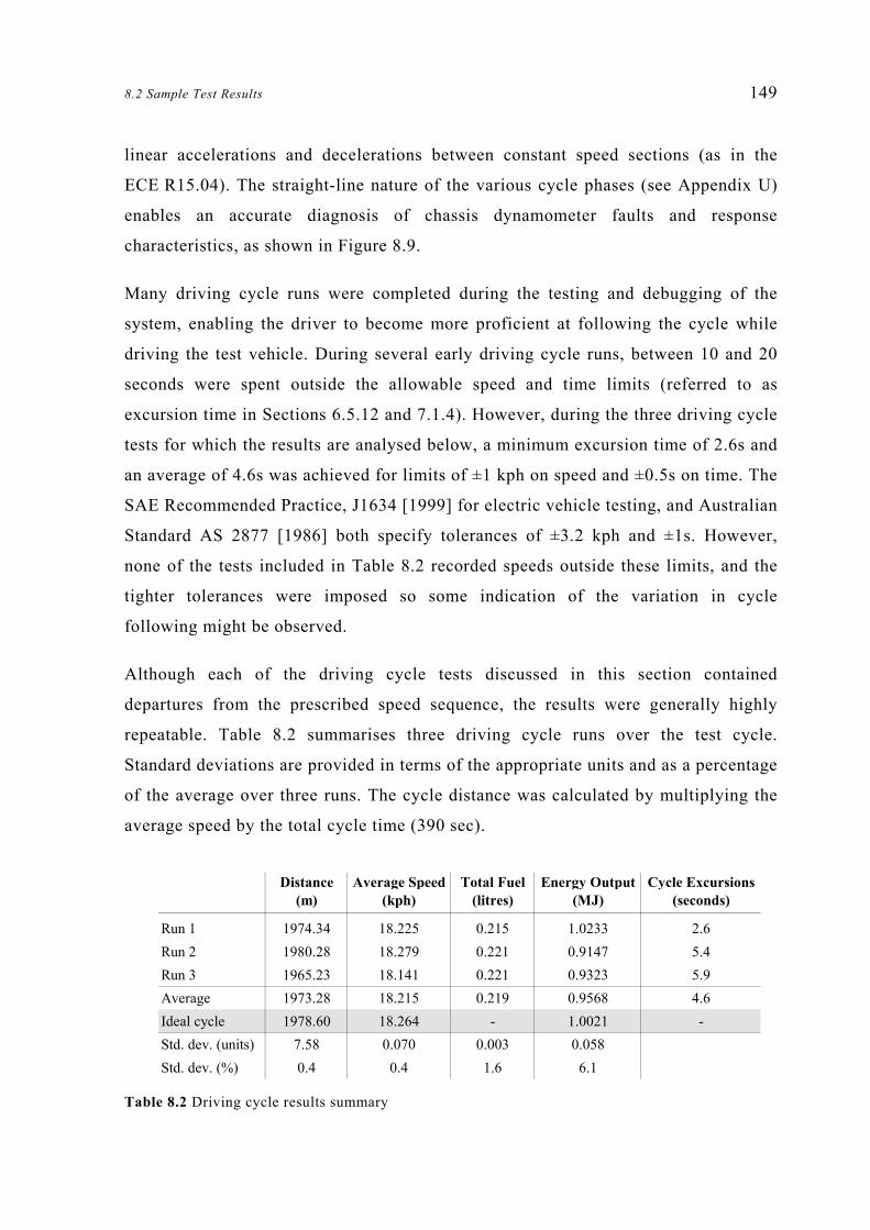
8.2 Sample Test Results 149
linear accelerations and decelerations between constant speed sections (as in the
ECE R15.04). The straight-line nature of the various cycle phases (see Appendix U)
enables an accurate diagnosis of chassis dynamometer faults and response
characteristics, as shown in Figure 8.9.
Many driving cycle runs were completed during the testing and debugging of the
system, enabling the driver to become more proficient at following the cycle while
driving the test vehicle. During several early driving cycle runs, between 10 and 20
seconds were spent outside the allowable speed and time limits (referred to as
excursion time in Sections 6.5.12 and 7.1.4). However, during the three driving cycle
tests for which the results are analysed below, a minimum excursion time of 2.6s and
an average of 4.6s was achieved for limits of ±1 kph on speed and ±0.5s on time. The
SAE Recommended Practice, J1634 [1999] for electric vehicle testing, and Australian
Standard AS 2877 [1986] both specify tolerances of ±3.2 kph and ±1s. However,
none of the tests included in Table 8.2 recorded speeds outside these limits, and the
tighter tolerances were imposed so some indication of the variation in cycle
following might be observed.
Although each of the driving cycle tests discussed in this section contained
departures from the prescribed speed sequence, the results were generally highly
repeatable. Table 8.2 summarises three driving cycle runs over the test cycle.
Standard deviations are provided in terms of the appropriate units and as a percentage
of the average over three runs. The cycle distance was calculated by multiplying the
average speed by the total cycle time (390 sec).
Table 8.2 Driving cycle results summary
Distance Average Speed Total Fuel Energy Output Cycle Excursions(m) (kph) (litres) (MJ) (seconds)
Run 1 1974.34 18.225 0.215 1.0233 2.6Run 2 1980.28 18.279 0.221 0.9147 5.4Run 3 1965.23 18.141 0.221 0.9323 5.9Average 1973.28 18.215 0.219 0.9568 4.6Ideal cycle 1978.60 18.264 - 1.0021 -Std. dev. (units) 7.58 0.070 0.003 0.058Std. dev. (%) 0.4 0.4 1.6 6.1

150 CHAPTER 8: Vehicle Testing Procedure and Sample Results
The total distance travelled (numerically integrated from the velocity record) and
average speed over the entire cycle were both within 0.3% of the actual driving cycle
values, and exhibited excellent repeatability between runs. However, energy output
totals were 4.5% lower on average than the value predicted by the vehicle energy
consumption modelling routine discussed in Section 7.2 (using an idle power of
1000 W). In addition, significant variations about the mean energy were experienced.
Initially, dynamometer lag (as shown in Figure 6.17) was thought to be the cause of
these lower energy totals. However, the inertial load compensated for by the power
absorber was relatively small, and the error introduced by this delay in the onset of
dynamometer load was estimated at less than 5000 J (0.005 MJ). Selection of idle
power may also affect this result, although it was thought that small changes in idle
power magnitude would not have a major effect, since both the actual and modelled
energy values take this into account in the same way. A more likely cause for the
higher energy prediction was in the assumption of vehicle mass (including the
rotational inertia approximation), which has consequences during the MATLAB
modelling of the ideal energy output, as well as the flywheel settings and
dynamometer driving cycle road load calculation. Trial and error adjustment of
vehicle mass may lead to a closer estimate of the driving cycle energy output.
Figure 8.9 gives an example of a typical driving cycle sequence, showing the
accuracy of the speed following, the engine speed, and fuel flowrate over a brief time
period. All three plots show the same time interval for a single test, so response times
can be observed by comparing vertically. The section of the cycle selected includes a
constant acceleration from stationary in first gear, then a change into second gear
followed by another acceleration and a constant speed period (in third gear). Figure
8.9a demonstrates several of the key issues in driving cycle demand following on the
dynamometer. All points on this speed plot are within the allowable speed and time
limits (±1 kph, and ±0.5s) although the departures at the 249 sec and 257 sec appear
to be close to these limits. The oscillations observed between 257 sec and 260 sec
were produced as a rapid decrease in acceleration (0.94–0 m/s2) excited torsional
vibrations in the chassis dynamometer shaft. In general, the most difficult portions of
a driving cycle for the driver were accelerating from stationary, and changing gears
before a constant speed section (as illustrated at 257 sec). Constant decelerations

8.3 Dynamometer System Performance 151
under braking (not shown) and accelerations at higher speeds (252–256 sec) lead to
less cycle excursions than the aforementioned speed demands.
Engine speed is presented in Figure 8.9b, which shows some of the electrical noise
blips and variations that were typical of the inductive loop spark plug pickup. Engine
revolutions per minute can be seen to rise and fall as the accelerator and clutch are
applied to engage first gear (244–247 sec), second gear (251–252 sec), and third gear
(257–258 sec). As expected, engine speeds vary according to road speed when the
clutch is engaged during acceleration and constant speed sections.
Fuel flowrate as measured by the Fluidyne flowmeter (see Appendix C.6 for set up) is
shown in Figure 8.9c. A predictable relationship between engine speed and fuel
flowrate is observed with minimal lag during the rapid transients enforced by gear
changes (compare engine rpm and fuel flowrate at 250–252 sec and 256–257 sec).
The apparently slow decrease in flowrate following the shift to third gear (257 sec)
was attributed to the increased power output (without significant change in engine
speed) as the vehicle accelerated between 257 sec and 259 sec. The noise present in
the Fluidyne flowmeter signal was typical of results during testing, but was not
thought to be restrictive, as fuel flowrate values are usually averaged. Table 8.2
includes the average and standard deviation of the fuel consumption over the three
sample driving cycle runs. The figure is expressed here in terms of total fuel
consumed in litres, which is integrated from the average flowrate, and converted
using the specific gravity of the fuel (0.743 kg/l). The standard deviation of 1.6%
represents acceptable repeatability, and the 0.22 litres of fuel consumed equates to an
average of 9.0 km/l. Fuel flowrate values over the course of the driving cycle testing
reached a maximum of 1.60 gm/s at 49 kph in third gear. This flowrate and speed
corresponds to a load of approximately 1200 N in the vehicle maps shown in Figures
8.4 and 8.5.
8.3 Dynamometer System Performance
This section gives an indication of the chassis dynamometer performance, in terms of
equipment and software, based on the proving tests discussed in Section 8.2.

152 CHAPTER 8: Vehicle Testing Procedure and Sample Results
242 244 246 248 250 252 254 256 258 260 262 264 266 268-5
0
5
10
15
20
25
30
35
40
Time (sec)
Spe
ed (
kph)
Measured speed & Desired speed
Cycle speed Measured speed
a.)
242 244 246 248 250 252 254 256 258 260 262 264 266 2680
200
400
600
800
1000
1200
1400
1600
1800
2000
2200
Time (sec)
Eng
ine
Spe
ed
(rpm
)
Engine Speedb.)
242 244 246 248 250 252 254 256 258 260 262 264 266 2680
0.25
0.5
0.75
1
1.25
1.5
Time (sec)
Fue
l Flo
wra
te (
gm/s
)
Fuel Flowrate c.)
Figure 8.9 Sample driving cycle sections a.) Cycle speed and measured speed b.) Engine speed
c.) Fuel flowrate

8.3 Dynamometer System Performance 153
8.3.1 Chassis Dynamometer Capacity
The 1982 Toyota Celica used during testing was considerably older than the average
passenger car in New Zealand at the time of writing. Newer vehicles, particularly
high performance automobiles, were expected to significantly exceed the maximum
power output of the test vehicle. Also, testing with larger vehicles such as light
trucks may be desired in the future, which would require a greater equivalent mass
from the flywheels.
In terms of speed, the maximum velocity attempted in the sample mapping tests was
100 kph. The dynamometer flywheels are rated to 120 kph, and lower gears may be
engaged on the test vehicle to decrease the maximum speed requirement. Speeds up
to 200 kph may be reached with no flywheels attached. It was expected that no
driving cycles representing New Zealand conditions would contain speed demands in
excess of 120 kph, and a maximum road load simulation speed of 120 kph was
thought to be sufficient.
The chassis dynamometer was originally designed for a maximum power absorption
of 300 kW, which is determined by the capacity of the Froude eddy-current
dynamometer. The test vehicle produced less than 60 kW (20% of capacity), and it is
again expected that most non-specialist applications will fall within the rated
maximum power. Similarly, the maximum tractive effort recorded during testing was
approximately 2200 N, representing less than 25% of the 10 000 N for which the
drum axle load cell may be calibrated. To enhance A/D resolution and calibration
accuracy, the signal was amplified such that a maximum of 5000 N tractive effort
could be read in, although this setting may be changed if future applications demand
greater tractive forces.
The mass of the test vehicle was assumed to be 1150 kg, which was increased to
1290 kg with the addition of driver and fuel weight, as well as a rotational inertia
approximation. A flywheel configuration used during driving cycle testing lead to an
equivalent mass of 1234 kg for the chassis dynamometer as a whole, which is 69% of
the maximum 1794 kg. A range of simulated masses between 664 kg and 1794 kg can
be achieved on the chassis dynamometer, which should be sufficient for most
passenger cars and some light trucks.

154 CHAPTER 8: Vehicle Testing Procedure and Sample Results
A maximum fuel consumption of less than 5 gm/s was recorded on the test vehicle,
whereas the Fluidyne flowmeter is rated up to 20 gm/s. Two Annubar tubes are
available to be combined with one of two pressure transducers for the measurement
of air flowrates to the vehicle engine. The smaller of the two pressure transducers
measures pressures up to 152 mmH2O, which equates at standard atmospheric
conditions to 52 gm/s using the small Annubar tube and 134 gm/s using the larger
tube. The larger pressure transducer measures up to 762 mmH2O, which allows
117 gm/s or 467 gm/s depending on which Annubar tube is utilised. The maximum
test vehicle air intake flowrate was approximately 70 gm/s, and was measured using
the larger Annubar tube, with the lower capacity pressure transducer, allowing plenty
of scope for greater flows.
8.3.2 Software Performance
Most of the major software processes are conducted in the MATLAB post-processing
suite, for the analysis of driving cycles and the plotting of vehicle mapping tests. The
calculations of total distance travelled and total fuel consumed consist of numerical
integrations using a two-point Newton-Cotes (Trapezium) scheme. The average rate
over each time interval is calculated and multiplied by the length of the interval. The
result is a step-by-step linear approximation of the area beneath the rate curve, which
may be prone to error in the presence of rapid changes in rate. However, the
repeatability of the fuel consumption and total distance figures quoted in Table 8.2
confirms that—given the cycle-following excursions—the numerical integration
technique is satisfactory.
The computer processing time is also of interest, since calculated data is usually
required as soon as possible. Programs that were required to traverse the 3901 data
points of the test driving cycle file tended to create the greatest delays. For example,
opening a driving cycle file and loading all the measured parameters into the
appropriate arrays (as per Section 7.1.2) took 17 seconds with the test driving cycle.
The vehicle energy consumption routine required 18 seconds to calculate the power
at each driving cycle point, compare it to the idle power, and add the energy output to
the cumulative total.
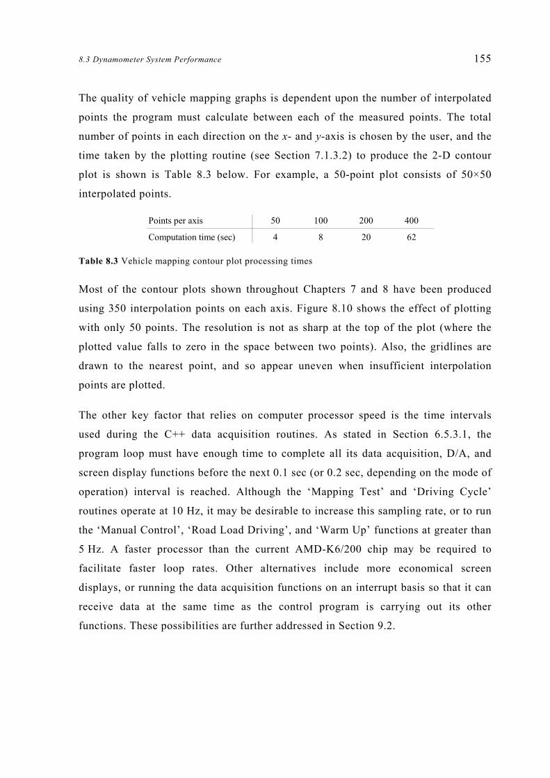
8.3 Dynamometer System Performance 155
The quality of vehicle mapping graphs is dependent upon the number of interpolated
points the program must calculate between each of the measured points. The total
number of points in each direction on the x- and y-axis is chosen by the user, and the
time taken by the plotting routine (see Section 7.1.3.2) to produce the 2-D contour
plot is shown is Table 8.3 below. For example, a 50-point plot consists of 50×50
interpolated points.
Table 8.3 Vehicle mapping contour plot processing times
Most of the contour plots shown throughout Chapters 7 and 8 have been produced
using 350 interpolation points on each axis. Figure 8.10 shows the effect of plotting
with only 50 points. The resolution is not as sharp at the top of the plot (where the
plotted value falls to zero in the space between two points). Also, the gridlines are
drawn to the nearest point, and so appear uneven when insufficient interpolation
points are plotted.
The other key factor that relies on computer processor speed is the time intervals
used during the C++ data acquisition routines. As stated in Section 6.5.3.1, the
program loop must have enough time to complete all its data acquisition, D/A, and
screen display functions before the next 0.1 sec (or 0.2 sec, depending on the mode of
operation) interval is reached. Although the ‘Mapping Test’ and ‘Driving Cycle’
routines operate at 10 Hz, it may be desirable to increase this sampling rate, or to run
the ‘Manual Control’, ‘Road Load Driving’, and ‘Warm Up’ functions at greater than
5 Hz. A faster processor than the current AMD-K6/200 chip may be required to
facilitate faster loop rates. Other alternatives include more economical screen
displays, or running the data acquisition functions on an interrupt basis so that it can
receive data at the same time as the control program is carrying out its other
functions. These possibilities are further addressed in Section 9.2.
Points per axis 50 100 200 400
Computation time (sec) 4 8 20 62

156 CHAPTER 8: Vehicle Testing Procedure and Sample Results
Figure 8.10 50-point interpolation plot of NOX concentration (c.f. Figure 8.6)

CHAPTER 9:
Future Work and Potential Improvements
9.1 Hardware Improvements
Electrical noise is always a consideration in data acquisition systems. In the chassis
dynamometer laboratory, there are two main causes of noise for the data acquisition
system: the physical path of the current wiring, and the ineffective earthing of several
devices. The display pendant arm that houses the driver’s monitor and keyboard also
carries potentiometers for manual control of the electric motor and dynamometer, as
well and load cell and speed feedback gauges. In addition, the data signal wires for
the engine spark pulses, vehicle thermocouples, and fuel flowrate (among others) are
connected to the data acquisition system via the pendant arm, which necessitates a
significant length of wiring from the end of the arm to wall, across the roof and into
the control room.
Plate 9.1 Electrical wiring path from driver’s pendant arm across laboratory roof

158 CHAPTER 9: Future Work and Potential Improvements
This length acts as an aerial of sorts, picking up interference from outside sources as
well. In addition, several floating ground loops exist within the various devices,
including the electric motor and power absorber. A common earth should be
established between each of the chassis dynamometer instruments, so that ground
noise is less of a factor. Alternately, isolation amplifiers could be installed to avoid
signal interference.
As mentioned in Section 8.2.3.3, the only exhaust emissions parameter measured
during the proving tests was the concentration of oxides of nitrogen. Also, the pump
servicing the Beckman NOX meter appeared to be overheating, and may require some
repair work. In future it is expected that all the original exhaust emissions equipment
owned by the University of Canterbury Mechanical Engineering Department will be
used for chassis dynamometer testing. The cabinet has recently been placed in an
appropriate location in the automotive lab, and requires connection of the necessary
A/D signal wires, and recalibrating of the CO, CO2, and HC meters individually.
Section 4.3.1 details the unsatisfactory response of the dynamometer load cell to
changes in temperature. Commercial load cells should be equipped with some form of
temperature compensation. However, susceptibility of both the eddy-current
dynamometer and roller drum load cells to temperature change suggests that these
devices are faulty and in need of replacement. The age of these load cells—each over
20 years—may also be contributing to the hysteresis that has been observed in the
measurement of dynamometer torque and tractive effort. In addition, problems
achieving certain loads during vehicle mapping (see Section 8.2.3.2) were thought to
be related to static friction in the tractive effort load cell linkage. Replacement of the
load cell may reduce these difficulties, and further investigation into the linkage
friction is recommended.
9.2 Data Acquisition Program
The most obvious improvement to the user interface and data acquisition program
would be to operate in a Windows environment, as opposed to the current DOS
format, which uses the Turbo Vision graphical user interface. The advantages of such
a system would include: a user-friendly and familiar appearance, superior memory

9.2 Data Acquisition Program 159
management capability, and the capacity to provide data graphing immediately,
without the use of additional post-processing applications such as MATLAB.
However, switching to a Windows application would require a complete revision of
the current source code, and also introduces timing difficulties as discussed in
Section 6.2. In either case, the addition of a ‘help’ function would greatly enhance
the usability of the system, especially for untrained operators. The memory
constraints imposed by the 20-bit addressing of DOS applications meant that a
comprehensive context-specific help—although achievable using Turbo Vision—was
not possible for the current chassis dynamometer C++ programs.
Section 6.5.11 includes a description of the vehicle mapping procedure, in which the
speed is held constant by the power absorber while each desired tractive effort
demand is met in turn. This method requires the driver to control for tractive effort
using the accelerator, which is not as natural a function as the speed holding
accomplished by a driver on the road. In addition, control of the power absorber in
torque mode was found to slightly be more stable than speed control, which was
unexpected, and most likely a result of the tuning of their respective analogue
controller potentiometers. An alternate mapping configuration calls on the driver to
maintain the set speed with each descending load applied by the dynamometer. This
method is more difficult at the maximum tractive effort points, as the power absorber
torque must be set on a trial and error basis. Using the current system the speed
control demand is maintained while the driver increases the load, until maximum
throttle is applied, at which point the achieved tractive effort is recorded. With the
dynamometer in torque control mode, the maximum tractive effort would be found by
applying full throttle and adjusting the power absorber load until the speed began to
drop away. It was thought that this adjustment could not easily be carried out under
computer control, although future investigation may produce a stable routine.
Another important factor is the speed at which the computer operations are carried
out. A faster processor may facilitate an increase in sampling rate, particularly during
Manual Control and Road Load Driving modes, which are currently updated at the
rate of 5 Hz. More efficient—or perhaps lower level—code may also enable faster
sampling of A/D data, and user feedback on screen. Without introducing a faster

160 CHAPTER 9: Future Work and Potential Improvements
processor, the current routines may be improved by decreasing the amount of data
displayed on-screen, or operating the data acquisition functions independently of the
main program loop. With the use of hardware timing and interrupts, the PCL-812PG
can perform data sampling functions at the same time as the computer processor is
operating on the other program code. This would provide a significant improvement
on the current scheme, which starts the data acquisition function, then waits until it is
complete before continuing. However, there may be some difficulties implementing
separate interrupt-based data sampling of the PCLD-889 daughter board, which
requires a different digital output from the computer (via the PCL-812PG) to switch
between each of the multiplexed channels.
Writing of the sampled data to a file also limits the operating speed of the control
program. During each data acquisition loop, the new data is written to a predefined
file, which is stored on the computer hard drive. A finite time period is required for
the head to access any given location on the hard disk. This data-saving time period
may be greatly reduced by saving to a temporary file in the computer’s random
access memory (RAM) during data recording processes. An imaginary drive may be
created in RAM, which can be saved to in exactly the same way as the hard drive, or
a floppy disk, but without the head-tracking time required for these operations. After
the test run is complete, the data may be transferred from the temporary file to a file
on the hard drive for permanent storage.
9.3 Post-Processing Software
The MATLAB calculation and plotting routines described in Chapter 7 have been
used effectively to produce the results contained in Chapter 8, and may continue to
be used without alteration. However, the stand-alone vehicle energy consumption
modelling (VECM) program could be improved. At the present time, the VECM
routine reads data from single-column files of cycle speeds or power measurements.
These files must be manually ‘cut-and-pasted’ from the full test data files, which
contain header information and recorded data from all the measured parameters. The
addition of the VECM functionality to the existing suite of post-processing routines
would enable menu-driven file selection and the reading of data from complete test
data files.

CHAPTER 10:
Conclusion
The University of Canterbury chassis dynamometer has been described in this thesis,
including the physical system configuration, inertia and friction calibration
techniques, and control software. Although equipped to do so, the chassis
dynamometer had not been used under computer control since being shifted to its
present location in the Mechanical Engineering Department automotive laboratory.
The work detailed in this thesis involved the preparation of the equipment for vehicle
testing, and the accompanying software required to record and analyse test results.
With reference to the system equations of motion, various methods of determining
the chassis dynamometer inertia and frictional characteristics have been described.
Simultaneous solving of several coastdown runs was selected as the most appropriate
method of inertia and friction determination in light of the performance of the ASEA
electric motor, especially at low speeds. The inertia of the roller drum assembly has
also been found by a similar method, enabling accurate representation of vehicle
tractive force using the drum axle load cell.
Data acquisition and dynamometer user interface software has been written in C++,
and has been described with reference to the memory constraints, and Turbo Vision
visual display format that is a feature of this DOS application. The data sampling,
digital-analogue demands, writing to file, and screen updates are timed using a
Universal Pulse Processor card, and occur at 0.2 sec or 0.1 sec intervals depending on
the mode of operation. Routines were created for warming up of the chassis
dynamometer and vehicle, and for general testing, including a function which enables
full throttle accelerations for determining maximum vehicle power output at the road
wheels.

162 CHAPTER 10: Conclusion
The ‘Mapping Test’ function allows the user to produce a map of vehicle
performance over a wide range of tractive effort loads and speeds. The software
program also includes a driving cycle routine, which allows a driver to execute speed
patterns in a vehicle on the dynamometer by following a scrolling demand trace on
the display monitor. Allowable speed and time errors may be specified, and sample
tests using a driving sequence based on the ECE R15.04 urban cycle indicated that
zero error speed following was possible, within certain limits.
Several data analysis and calculation programs have been written using MATLAB,
and the program structure has been described, including the available menus and how
the selected files are read into matrices from which they may be edited or graphed.
Specialised routines are available for the plotting of the maximum power curves and
vehicle mapping tests displayed throughout this thesis. Software has also been
written for the purpose of comparing the ideal driving cycle power with measured
outputs. The predicted total energy output was found to be 4.5% greater than the
average energy consumption calculated from several test runs.
Vehicle power, mapping and driving cycle tests were conducted using a 1982 Toyota
Celica, with a view to determining the accuracy and repeatability of the chassis
dynamometer. Maximum power at the road wheels was determined in several full-
throttle acceleration tests, which yielded peak power measurements with a standard
deviation of 1.0%. Mapping tests were also carried out on the test vehicle to
determine the instrumentation accuracy and suitability of the method in general.
Satisfactory repeatability was observed for the measurement of velocity, fuel
flowrate, dynamometer torque and tractive effort. Calculations of fuel consumption,
thermal efficiency and energy consumption also yielded standard deviations of
approximately 1%. However, the Annubar air flowrate equipment exhibited some
unpredictability, and substandard results were obtained from the Beckman NOX
meter. The latter was thought to be the result of a blockage in the system, which may
be remedied by overhauling the sample pump. Driving cycle data also proved to be
sufficiently repeatable for meaningful testing to be conducted on the chassis
dynamometer. For the three test cycle runs discussed in Chapter 8, the average
163
vehicle speed was within 0.05 kph of the prescribed cycle average, and the total fuel
consumption figures exhibited a standard deviation of 0.003 litres (1.6%).
The inability of the Froude eddy-current power absorber to generate torque at zero
velocity lead to the implementation of a software routine—included in the driving
cycle dynamometer demand calculation—that disabled the demand output during
deceleration or stationary periods. A 2 second lag in power absorber response was
still evident, but overshoot was decreased by 90% in some cases and it was thought
that the dynamometer provided satisfactory road load simulation for effective driving
cycle testing.
Several key improvements to the system have been suggested in Chapter 9, including
rewiring to decrease signal interference, and a number of ways in which the
processing time required by the data acquisition routine could be minimised.
However, the chassis dynamometer system has all the necessary hardware and
software for a wide variety of focussed vehicle testing. In the future, it is expected
that the chassis dynamometer will be used in the development of alternative fuels and
new vehicle technologies, as well as tuning and performance tests on existing cars
and light trucks.


References
AS 2877 (1986) Methods of Test for Fuel Consumption of Motor Vehicles Designed
to Comply With Australian Design Rules 37 and 40. Standards Association of
Australia
AutoData Ltd. (1990) Technical Data: Tune Up and Specifications for Passenger
Cars and Light Commercial Vehicles. Maidenhead (England)
Burke, C.E., Nagler, L.H., Campbell, E.C., Zierer, W.E., Welch, H.L., Lundstrom,
L.C., Kosier, T.D., McConnell, W.A. (1957) Where Does All the Power Go?
S.A.E. Transactions, 65
Castro, F.A. (1989) Automobile Fuel Consumption Estimates: ECE and EPA versus
Real World. Proceedings of a seminar organised by the commission of the
European Communities, Directorate General for Energy, May 1988
Coomber, I.M. (1988) Toyota Celica Owners Workshop Manual : (Feb 1982 to Sept
1985, all models, 1972cc). Sparkford, Nr. Yeovil, Somerset, England : Haynes
Elliot, D.R., Klamp, W.K., Kraemer, W.E. (1971) Passenger Tire Power
Consumption. S.A.E. Transactions No. 710575
Epps, I.K. (1987) Vehicle Energy Consumption Modelling. University of Canterbury
Department of Mechanical Engineering, Final Year Project 1987/63
Fraleigh, J.B., Beauregard, R.A. (1990) Linear Algebra. (2nd Edition) Addison-
Wesley Publishing Company
Franklin, G.F., Powell, J.D., Emami-Naemi, A. (1994) Feedback Control of Dynamic
Systems. (3rd Edition) Addison-Wesley Publishing Company
Froude Consine (2001) Website: www.fki-eng.com/index.cfm?company=fc
166 CHAPTER 10: References
Hindin, P.J. (1984) Comparison of Fuel Consumption Driving Patterns. University of
Canterbury Project 710/05/2
Hindin, P.J. (1985) The Determination of Motor Vehicle Road Load. Master of
Engineering Thesis, Department of Mechanical Engineering, University of
Canterbury
Hindin, P.J. (1986) Vehicle Driveability Assessment using a Chassis Dynamometer.
IPENZ Transactions Vol.13 No.3/EMCh
NZS 5420 [withdrawn] (1980) Methods of Test for Fuel Consumption of Cars.
Standards Association of New Zealand
Raine, J.K. (1981) The Design of a Chassis Dynamometer for Programmable Vehicle
Testing. NZIE Transactions Vol.8 No.1/EMCh
Rototest (2001) Website: www.chassisdynamometer.com
SAE J1082 (1995) Fuel Economy Measurement Road Test Procedure. SAE Standard,
Jun95. Society of Automotive Engineers, Inc.
SAE J1263 (1996) Road Load Measurement and Dynamometer Simulation using
Coastdown Techniques. SAE Recommended Practice, Feb96. Society of
Automotive Engineers, Inc.
SAE J1506 (1993) Emission Test Driving Schedules. SAE Information Report,
Apr93. Society of Automotive Engineers, Inc.
SAE J1634 (1999) Electric Vehicle Energy Consumption and Range Test Procedure.
SAE Recommended Practice, Apr99. Society of Automotive Engineers, Inc.
Schenck Pegasus GmbH (2001) Website: www.schenck.net/PEGASUS/indexe.htm
Taylor Dynamometer (2001) Website: www.taylordyno.com
Wheeler, D.J. (1963) Principles of Vehicle Selection. S.A.E. Transactions, 71.
White, R.A., Korst, H.H. (1972) The Determination of Vehicle Drag Contributions
from Coastdown Tests. SAE Technical Paper Series 720099.

167
APPENDIX A:
Flywheel Equivalent Mass Combinations
The table below shows all the possible equivalent mass increments that may be
achieved with the chassis dynamometer flywheel set. Asterisks indicate that the
flywheel (or hollow shaft) is engaged. A description of the flywheel set is included in
Section 2.2.
Table A.1 Flywheel combinations and resultant equivalent masses
Hollow 110 220 230 450 Equivalentshaft kg kg kg kg mass (kg)
664
* 784
* * 894
* * 1004
* * * 1114
* * * 1234
* * * * 1344
* * * 1454
* * * * 1574
* * * * 1684
* * * * * 1794


169
APPENDIX B:
Comparison of Chassis Dynamometer Specifications
See Table B.1 overleaf.
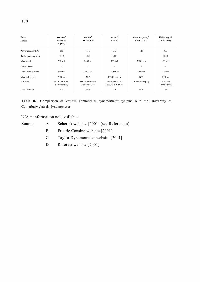
170
Table B.1 Comparison of various commercial dynamometer systems with the University of
Canterbury chassis dynamometer
N/A = information not available
Source: A Schenck website [2001] (see References)
B Froude Consine website [2001]
C Taylor Dynamometer website [2001]
D Rototest website [2001]
Brand SchenckA FroudeB TaylorC Rototest (VPA)D University ofModel EMDY 48 48 CM CD CM 90 620 F1 2WD Canterbury
(X-Drive)
Power capacity (kW) 150 150 373 628 300
Roller diameter (mm) 1219 1220 900 — 1200
Max speed 200 kph 200 kph 137 kph 3000 rpm 160 kph
Driven wheels 2 2 4 2 2
Max Tractive effort 5400 N 4500 N 10800 N 2000 Nm 9150 N
Max Axle Load 2000 kg N/A 11340 kg/axle N/A 8000 kg
Software MS Excel & in- MS Windows NT Windows-based Windows display DOS C++house display / modular C++ ENGINE Vue ™ (Turbo Vision)
Data Channels 150 N/A 24 N/A 16

171
APPENDIX C:
Instrument Calibrations
C.1 Froude Eddy-Current Dynamometer Load Cell
Output: ±10 V
A/D configuration: PCL-812PG ±10 V
Estimated measurement uncertainty: ±1 Nm
Static calibration was first carried out with the dynamometer load cell in
compression. That is, in the direction of positive rotation as defined in Chapter 3.
The A/D signal was recorded as each known mass was added sequentially then
removed from the dynamometer calibration arm. The linear fit was calculated using a
least squares approximation.
500 1000 1500 2000
0
100
200
300
400
500
600Dynamometer Load Cell in Compression
A/D signal (bits)
App
lied
Torq
ue (N
m)
Table C.1 and Figure C.1 Dynamometer load cell calibration in compression
( ) ( )ConstantZero+×−= bitsNmTorquenCompressio 0.3766 (C-1)
Note: The Zero Constant (772.1 during calibration) is replaced when rezeroing the
load cell to account for temperature differences (see Section 4.3.1).
Total Mass Torque A/D signal(kg) (Nm) (bits)
0.00 0.00 205022.68 113.35 175145.32 226.53 145168.00 339.91 114990.64 453.11 848
113.36 566.66 54590.64 453.11 84668.00 339.91 114745.32 226.53 144822.68 113.35 17490.00 0.00 2049

172
The error in this A/D measurement was determined by calculating the difference
between the load cell torque (as determined by Equation C-1) and the actual applied
torque. The following graph shows the hysteresis evident during these static
calibrations. Also, it was apparent that the calibration multiplier and constant
(-0.3766 and 772.1 above) in compression were not appropriate for use when the load
cell was in tension.
-600 -400 -200 0 200 400 600-2
-1.5
-1
-0.5
0
0.5
1
1.5
2
2.5Calibration Error using Compression Coefficents
Applied Torque (Nm)
Err
or in
Cal
cula
ted
Torq
ue (N
m)
COMPRESSION TENSION
Figure C.2 Dynamometer load cell A/D error using compression calibration coefficients
A separate calibration equation was sought for the load cell in tension (by placing
masses on the other side of the calibration arm). During everyday dynamometer
operation, the user inputs the expected direction of roller motion during the rezeroing
process. The new zero point is then used with the appropriate calibration multiplier in
subsequent torque calculations.
2000 2500 3000 3500
-600
-500
-400
-300
-200
-100
0
100Dynamometer Load Cell in Tension
A/D signal (bits)
App
lied
Torq
ue (N
m)
Table C.2 and Figure C.3 Dynamometer load cell calibration in tension
Total Mass Torque A/D signal(kg) (Nm) (bits)
0.00 0.00 2051-26.95 -134.72 2405-49.66 -248.25 2705-72.32 -361.51 3005-95.04 -475.11 3309
-117.72 -588.49 3609-95.04 -475.11 3310-72.32 -361.51 3010-49.66 -248.25 2710-26.95 -134.72 24100.00 0.00 2054
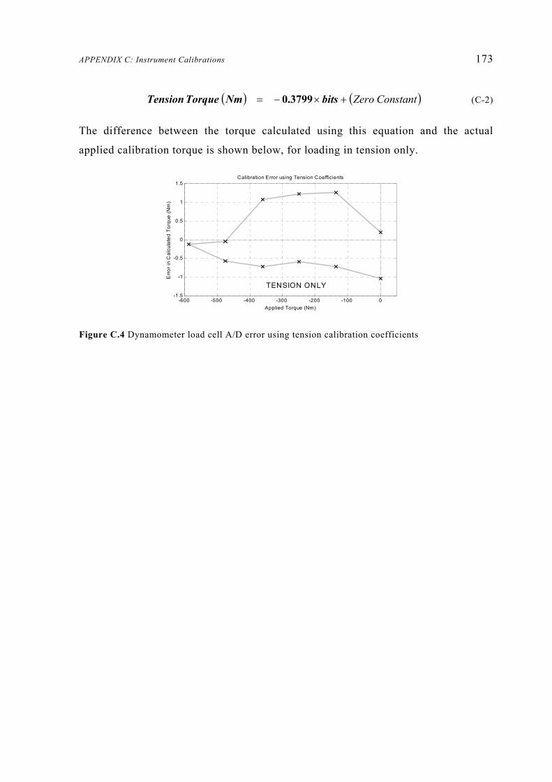
APPENDIX C: Instrument Calibrations 173
( ) ( )ConstantZero+×−= bitsNmTorqueTension 0.3799 (C-2)
The difference between the torque calculated using this equation and the actual
applied calibration torque is shown below, for loading in tension only.
-600 -500 -400 -300 -200 -100 0-1.5
-1
-0.5
0
0.5
1
1.5Calibration Error using Tension Coefficients
Applied Torque (Nm)
Err
or in
Cal
cula
ted
Torq
ue (N
m)
TENSION ONLY
Figure C.4 Dynamometer load cell A/D error using tension calibration coefficients

174
C.2 Froude Eddy-Current Dynamometer Demand Signal Calibration
Input: -10–0 V
Estimated output uncertainty: ±0.5 Nm in Torque control mode
± 3 kph in Speed control mode
The dynamometer control functions were calibrated using the C++ software routines
detailed in Chapter 6. A vehicle was driven on the chassis dynamometer to apply a
force at the rollers, which was resisted by the power absorber in either constant speed
or constant torque mode. Digital demand inputs were entered in 12-bit form (0–4095)
and sent as a negative voltage (-10–0V) to the power absorber by the PCL-812PG.
20 40 60 80 100 12050
100
150
200
250
300
350
400
450
500
550Dynamometer Torque Demand Calibration
Torque Output (Nm)
Dem
and
sign
al (b
its)
Table C.3 and Figure C.5 Dynamometer torque control D/A calibration
( ) 2.14.299 +×= TorqueDesiredBitsDemand (C-3)
Demand Torque(bits) (Nm)
200 46.93200 46.67200 46.17200 46.17100 22.28100 22.42100 22.43100 22.79350 80.82350 80.84350 80.82350 80.6500 115.9500 115.88500 115.83500 115.52
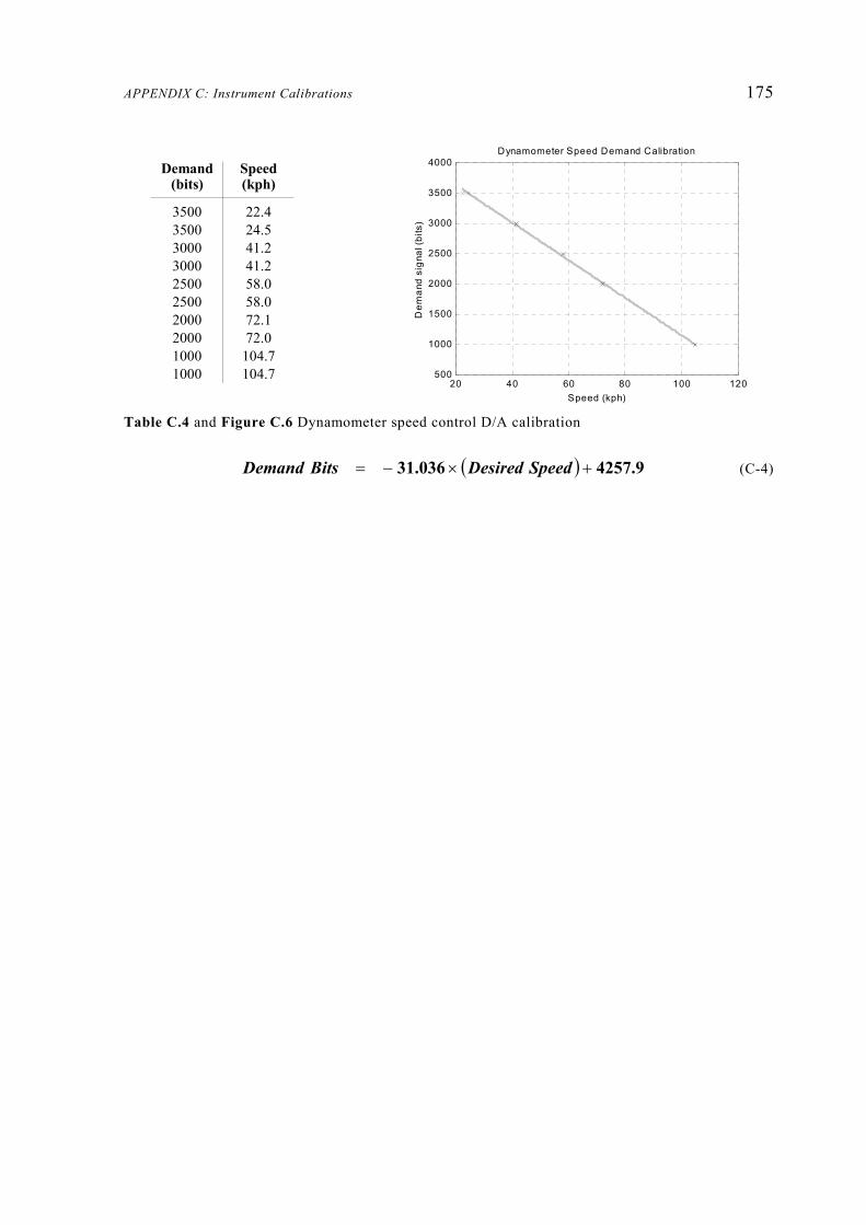
APPENDIX C: Instrument Calibrations 175
20 40 60 80 100 120500
1000
1500
2000
2500
3000
3500
4000Dynamometer Speed Demand Calibration
Speed (kph)
Dem
and
sign
al (b
its)
Table C.4 and Figure C.6 Dynamometer speed control D/A calibration
( ) 4257.931.036 +×−= SpeedDesiredBitsDemand (C-4)
Demand Speed(bits) (kph)
3500 22.43500 24.53000 41.23000 41.22500 58.02500 58.02000 72.12000 72.01000 104.71000 104.7

176
C.3 ASEA Electric Motor Load Cell
Output: ±5 V
A/D configuration: PCL-812PG ±5 V
Estimated measurement uncertainty: ±2.5 Nm
Static calibration was carried out on the electric motor load cell in both the positive
and negative directions. Positive motor torque occurs when the motor is applying a
force that will accelerate the chassis dynamometer when is it rotating in a positive
direction as defined in Chapter 2. The A/D signal (0–4095) was recorded as each
known mass was added sequentially then removed from the calibration arm. The
calibration arm may be loaded on either side at any one time, enabling positive and
negative torques to be measured.
0 1000 2000 3000 4000-250
-200
-150
-100
-50
0
50
100
150
200
250Motor Load Cell Calibration
A/D signal (bits)
App
lied
Torq
ue (N
m)
Figure C.7 Electric motor load cell calibration
( ) 250.90.1227 −×= bitsNmTorque (C-5)
Table C.5 Electric motor load cell calibration
Total Mass Torque A/D signal(kg) (Nm) (bits)
0.00 0.00 2048.65.00 24.53 2238.9
10.00 49.05 2435.515.00 73.58 2637.420.00 98.11 2834.325.00 122.64 3032.130.00 147.16 3233.535.00 171.69 3435.440.99 201.04 3681.544.97 220.60 3845.640.99 201.04 3686.335.00 171.69 3443.330.00 147.16 3241.425.00 122.64 3041.020.00 98.11 2842.915.00 73.58 2642.510.00 49.05 2440.65.00 24.53 2243.70.00 0.00 2051.9
0.00 0.00 2046.2-10.00 -49.05 1662.2-20.00 -98.11 1260.7-30.00 -147.16 851.9-35.00 -171.69 645.0-40.99 -201.04 397.5-44.97 -220.60 234.0-40.99 -201.04 393.7-35.00 -171.69 639.6-30.00 -147.16 845.6-20.00 -98.11 1253.2-10.00 -49.05 1655.20.00 0.00 2042.5

APPENDIX C: Instrument Calibrations 177
Errors during calibration were plotted as the difference between the applied torque,
and the torque calculated using the previous A/D equation.
-250 -200 -150 -100 -50 0 50 100 150 200 250-2
-1.5
-1
-0.5
0
0.5
1
1.5
2
2.5Calibration Error for Motor Load Cell
Applied Torque (Nm)
Err
or in
Cal
cula
ted
Torq
ue (N
m)
Figure C.8 Error in electric motor load cell A/D calibration in tension and compression
These errors may have been induced by a lack of concentricity in the system, and
could have been reduced by applying a cubic fit to the calibration data. However, to
simplify the data capture software, the linear approximation shown here was
maintained. Because the response of the electric motor precluded its use during
testing, a measurement uncertainty of ±2.5 Nm was thought to be acceptable.

178
C.4 ASEA Electric Motor Demand Signal Calibration
Input: ±10 V
Estimated output uncertainty: ± 2 Nm in Torque control mode
± 2 kph in Speed control mode
The ASEA electric motor was not used during testing (see Section 5.2.3), but
required calibration so that approximate torque and velocity states could be achieved
while warming up, or prior to dynamometer coastdown tests (see Chapter 6). Digital
demand inputs were entered in 12-bit form (0–4095) and sent as a voltage (±10 V) to
the electric motor by the PCL-812PG.
-50 0 50 100 150 200-200
0
200
400
600
800
1000
1200
1400
1600
Motor Torque Calibration
Torque (Nm)
A/D
Dem
and
(bits
)
Table C.6 and Figure C.9 Electric motor torque control D/A calibration
( ) 1.210.494 −×= TorqueDesiredbitsDemand (C-6)
With the exception of the zero demand points, motor torque was applied while under
constant speed control (50 kph) from the power absorber. Torque at zero motor
demand was measured at 50 kph while coasting down. The negative value at zero
torque is representative of the motor friction, which will vary with velocity. At
torque demands greater than zero, this friction is motored out and is indistinguishable
from the electromagnetic motoring torque, since a single measurement is made at the
motor load cell (see Chapter 5.1).
Demand Torque(bits) (Nm)
0 -1.72400 40.52800 77.85
1200 114.641600 151.781600 151.661200 114.57800 77.86400 40.24800 73.89
0 -1.43
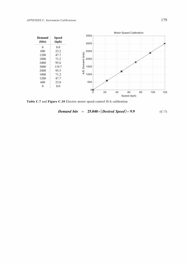
APPENDIX C: Instrument Calibrations 179
0 20 40 60 80 100 1200
500
1000
1500
2000
2500
3000
3500Motor Speed Calibration
Speed (kph)
A/D
Dem
and
(bits
)
Table C.7 and Figure C.10 Electric motor speed control D/A calibration
( ) 9.925.040 +×= SpeedDesiredbitsDemand (C-7)
Demand Speed(bits) (kph)
0 0.0600 23.2
1200 47.71800 71.22400 95.63000 119.72400 95.51800 71.21200 47.7600 23.0
0 0.0

180
C.5 Tractive Effort Load Cell
Output: ±10 V
A/D configuration: PCL-812PG ±5 V
Estimated measurement uncertainty: ±9 N
As described in Section 4.3.2, the hysteresis of the tractive effort load cell and its
associated linkage required a special calibration technique. Known masses were
added to the load arm while the roller drums were rotated slowly by the electric
motor. A vehicle was positioned on the rollers to prevent lifting of the drum axle
from its trunnion bearings. As with the power absorber load cell, it was found that
more accurate results could be obtained by calculating a different calibration
multiplier for each of the compression and tension states of the load cell. Also, poor
temperature compensation required that the load cell software be rezeroed to account
for day-to-day temperature differences. Thus, the constant component of the
calibration equations included here has been left as a variable. Equations are stated in
terms of A/D bits (i.e. 0–4095) with the PCL-812PG range set at ±5 V.
500 1000 1500 2000 2500
-1000
0
1000
2000
3000
4000
5000
6000Tractive Effort Load Cell in Compression
A/D Signal (bits)
App
lied
For
ce (N
)
Table C.8 and Figure C.11 Tractive effort load cell calibration in compression
ConstantZerobitsForcenCompressio +×−= 3.715 (C-8)
The error in this A/D measurement was determined by calculating the difference
between the load cell force (as determined by Equation C-8) and the actual applied
force.
Total Mass Force A/D signal(kg) (N) (bits)
0.00 0.00 204422.64 1110.25 174645.32 2222.80 144668.04 3337.46 114690.70 4448.74 846
113.41 5562.66 54690.70 4448.74 84568.04 3337.46 114545.32 2222.80 144422.64 1110.25 17440.00 0.00 2042
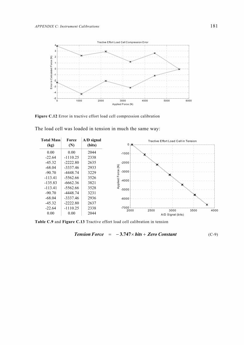
APPENDIX C: Instrument Calibrations 181
0 1000 2000 3000 4000 5000 6000-5
-4
-3
-2
-1
0
1
2
3
4Tractive Effort Load Cell Compression Error
Applied Force (N)
Err
or in
Cal
cula
ted
For
ce (N
)
Figure C.12 Error in tractive effort load cell compression calibration
The load cell was loaded in tension in much the same way:
2000 2500 3000 3500 4000-7000
-6000
-5000
-4000
-3000
-2000
-1000
0Tractive Effort Load Cell in Tension
A/D Signal (bits)
App
lied
For
ce (N
)
Table C.9 and Figure C.13 Tractive effort load cell calibration in tension
ConstantZerobitsForceTension +×−= 3.747 (C-9)
Total Mass Force A/D signal(kg) (N) (bits)
0.00 0.00 2044-22.64 -1110.25 2338-45.32 -2222.80 2635-68.04 -3337.46 2933-90.70 -4448.74 3229
-113.41 -5562.66 3526-135.83 -6662.36 3821-113.41 -5562.66 3528-90.70 -4448.74 3231-68.04 -3337.46 2936-45.32 -2222.80 2637-22.64 -1110.25 23380.00 0.00 2044

182
-7000 -6000 -5000 -4000 -3000 -2000 -1000 0-10
-8
-6
-4
-2
0
2
4
6Tractive Effort Load Cell Tension Error
Applied Force (N)
Err
or in
For
ce C
alcu
latio
n (N
)
Figure C.14 Error for tractive effort A/D calibration in tension
Note: Both points at zero load, and both at –1110.25 N, overlap in Figure C.14 due to
similar readings during adding and subtraction of calibration masses.

APPENDIX C: Instrument Calibrations 183
C.6 Fluidyne Fuel Flowmeter
Output: 0–5 V
A/D configuration: PCL-812PG ±5 V
Estimated measurement uncertainty: ±0.04 gm/s
Firstly, the flowrate and totaliser were tested against measured fuel quantities in
order to test the repeatability, and to set the correct fuel density on the meter’s
potentiometers. A pump was used to pass fuel from a tank, through the flowmeter,
through an adjustable valve, and into a container mounted on a set of electronic
scales. The total mass of fuel was weighed and compared to the total indicated on the
flowmeter digital display. Experiments were conducted over various time intervals
and flowrates, and a density setting of 743 kg/m3 was found to be appropriate.
Human error in starting and stopping the totaliser, as well as the measurement
uncertainty in the scales, led to an estimated error of ±0.2 gm at flowrates below
2 gm/s and ±1.0 gm at flowrates greater than 4 gm/s.
Table C.10 Flowmeter totaliser test results
The measurement accuracy for the total fuel reading was assumed to extend to the
flowrate, and an uncertainty of ±0.5% was combined with the A/D uncertainty shown
in Figure C.16. The A/D performance was assessed using a similar experimental set-
up, and comparing the flowrate—as indicated on the flowmeter’s digital display—
with the A/D signal recorded in terms of bits (0–4095) with a PCL-812PG range of
±5 V.
Nominal Flowrate Mass of Fuel Flowmeter Total Error Error Average Error(gm/s) (gm) (gm) (gm) (%) (%)
1.2 200 200.4 0.4 0.20200 200.2 0.2 0.10240 239.9 -0.1 -0.04 0.09
3.5 200 200.5 0.5 0.25200 200.3 0.3 0.15200 200.3 0.3 0.15 0.18
5.7 450 449.9 -0.1 -0.02450 448.1 -1.9 -0.42400 398.9 -1.1 -0.28400 398.6 -1.4 -0.35 -0.27

184
2000 2200 2400 2600 2800-1
0
1
2
3
4
5
6
7Fuel Flowrate Calibration
A/D Signal (bits)
Mea
sure
d F
low
rate
(g/s
)
Table C.11 and Figure C.15 Fuel flowmeter A/D calibration
( ) 20.050.009793 −×= bitsgm/sFlowrate (C-10)
† Note: Each point included in the above table represents the average of three points
recorded at the same flowrate.
The graph below shows the difference between the flowrate indicated by the meter,
and the flowrate calculated using the A/D signal.
0 1 2 3 4 5 6 7-8
-6
-4
-2
0
2
4
6
8x 10
-3 Fuel Flowrate Calibration Error
Flowrate (g/s)
Err
or in
Cal
cula
ted
Flo
wra
te (g
/s)
Figure C.16 Error in fuel flowmeter A/D calibration
The measurement uncertainty recorded previously (±0.5%) equates to ±0.025 gm/s at
a fuel flowrate of 5 gm/s (the largest rate encountered during the testing detailed in
Digital display A/D signal(gm/s) (bits)†
0.00 2047.00.34 2082.50.79 2128.11.52 2203.52.12 2264.52.83 2337.03.61 2416.64.08 2464.94.49 2506.54.80 2537.75.20 2578.45.68 2627.56.12 2672.66.36 2697.16.55 2716.46.60 2721.5

APPENDIX C: Instrument Calibrations 185
Chapter 8). Thus, the A/D uncertainty shown here (±0.007 gm/s) is the lesser of the
two sources of error. An overall uncertainty of ±0.04 gm/s was thought to be
sufficient to include meter accuracy and A/D conversion uncertainty for the measured
flowrates.
The MATLAB software routines detailed in Chapter 7 include the facility to calculate
the total fuel consumed during a test run. Because the digital outputs from the
Fluidyne flowmeter do not include the total mass, the flowrate must be numerically
integrated. A two-point Newton-Cotes (Trapezium) integration technique was used,
which calculates the fuel mass over each time interval thus:
Figure C.17 Integration of flowrate using the ‘Trapezium’ rule
Several tests were conducted to determine the effectiveness of this approximation.
The fuel was pumped, as per the calibration runs, with the flowrate being varied by a
valve. A combination of non-uniform variations (as in Figure C.18) and step changes
yielded an average error of 0.2% between the integrated total and the totaliser value
recorded by the flowmeter.
∆t
F2
F1
Time
( )2
21 tFFMass ∆×+=

186
0 10 20 30 40 50 60 70 80 90 100 110
0
1
2
3
4
5
6
7
8Fuel Flowrate Variation for Integration Test
Time (sec)
Flo
wra
te (g
/s)
F lowmeter total mass = 301.6 gIntegrated total mass = 301.9 g
Figure C.18 Example of non-uniform rate test for fuel flow integration
Inserting the Fluidyne flowmeter into the fuel systems of carburetted vehicles
involves making a break in the line, and connecting the device in series. Fuel-injected
engines often require a different approach. For example, in the case of the test
vehicle, the supply line provides fuel to the injector rail at a constant pressure, with a
flowrate greater than or equal to the maximum consumption of the engine. Fuel that
is not injected into the cylinders is returned to the tank via the return line. Unless
both the supply and the return flowrates can be measured simultaneously (by two
separate devices), the fuel consumption of the engine cannot be determined by simply
inserting a meter in series. A schematic arrangement of the Toyota Celica test vehicle
fuel system in Figure C.19 below. Figure C.20 shows the modified fuel flow path,
including the Fluidyne flowmeter and adjustable valve used to regulate the supply
pressure.
Figure C.19 Test vehicle original fuel system schematic
PUMP
TANK
INJECTOR RAIL SUPPLY LINE
RETURN LINE

APPENDIX C: Instrument Calibrations 187
Figure C.20 Test vehicle fuel system reconfigured to include flowmeter
By plugging the return line and providing a path back to the tank before the fuel
reaches the injectors, all the fuel passing into the injector rail (via the flowmeter) is
consumed by the engine. Insufficient pressure at the new return valve will result in
too much fuel flowing straight back into the tank. Pressure to the injectors is
maintained by adjusting the valve, and monitoring a pressure gauge in the supply
line.
REROUTED RETURN
PLUG (NO FLOW) REGULATING
VALVE
FLOWMETER
PRESSURE GAUGE

188
C.7 Annubar Flow Sensors with Dieterich Standard Pressure Transducers
Output: 4–20 mA
A/D configuration: PCL-812PG ±5 V
Estimated measurement uncertainty: ±2 gm/s
The two Annubar devices indicate the flowrate by measuring pressure and applying a
standard Annubar equation:
( ) ( )492
59
/+×
×=
amb
Annamb
T
ppConstantAnnubarhrkgFlow (C-11)
Where: pamb = Ambient air pressure (mb)
pAnn = Annubar pressure (mmH2O)
Tamb = Ambient air temperature (ºC)
The Annubar Constant is 10.99 for the small inlet tube (1.610 in), and 43.998 for the
large inlet tube (3.068 in). The validity of this relationship was confirmed by
measuring the average flow velocity using a Pitot tube. For these initial experiments,
the Annubar pressure was measured with a water manometer at relatively low
flowrates.
Table C.12 Flowrate measured using an Annubar compared to flowrate measured using a Pitot tube
The difference in flowrate between the two methods may have been brought about by
misalignment of the Pitot tube. This error would tend to decrease the velocity—and
hence flowrate—indicated by the Pitot tube arrangement. Thus, the error shown in
the table was thought to be a maximum, and it was assumed that the Annubar
pressure method was sufficiently accurate for chassis dynamometer work.
RUN Flow temp Air Pressure Pitot Average Pitot velocity Annubar Pressure Pitot Flowrate Annubar Flowrate Difference(°C) (mb) (mmH2O) (m/s) (mmH2O) (kg/hr) (kg/hr) (%)
1 17 1014.0 0 0 0 0 0 02 20 1013.4 0.785 3.58 1.16 64.98 65.65 1.013 23 1012.7 1.587 5.12 2.36 91.89 93.12 1.344 25 1012.1 2.498 6.45 3.85 114.88 118.52 3.07

APPENDIX C: Instrument Calibrations 189
In order to read the Annubar pressure, electronic transducers with a variable current
output were connected to the PCL-812PG A/D card. The air-flow measurement rig
includes two Dieterich Standard pressure transducers, which provide an output of
4–20 mA over pressure ranges of 0–6 and 0–30 inH2O respectively. A combination of
the large Annubar tube and the smaller transducer enabled flowrates up to
approximately 750 kg/hr (208 gm/s) under standard atmospheric conditions. The
maximum air flowrate for the test vehicle described in Chapter 8 was approximately
70 gm/s. Measuring the potential across a 560 Ω resistor at the A/D card, the
maximum voltage encountered during vehicle testing was 3.2 V.
With the PCL-812PG range set at ±5 V, the A/D output (0–4095) from the pressure
transducers was compared with the Annubar pressure, as measured by a water
manometer connected to the same pressure lines.
Table C.13 Annubar flowrate A/D calibration data
2800 3000 3200 3400 3600 3800 4000 4200-10
0
10
20
30
40
50Manometer presssure vs A/D output
A/D output (bits)
Ann
ubar
Pre
ssur
e (m
mH
2O)
Figure C.21 Annubar flowrate A/D calibration data
( ) 125.90.04281 −×= bitsPressure OmmH 2 (C-12)
This pressure can be converted to a flowrate in kg/hr or gm/s using the Annubar
equation on the previous page.
Pressure (mmH2O) 0 0.1 0.8 7.1 12.6 15.9 25.0 34.0 42.4 46.0A/D output (bits) 2939.0 2939.0 2958.9 3107.1 3242.5 3311.6 3528.7 3741.4 3927.1 4011.6

190
C.8 Airflow DB-1 Digital Barometer
Output: 0–1999 mV
A/D configuration: PCL-812PG ±1.25 V via PCLD-889
Estimated measurement uncertainty: ±4 mb
First, the digital display was related to the voltage output:
Table C.14 Barometer A/D signal calibration vs. display
0.96 0.97 0.98 0.99 1 1.01 1.02 1.03 1.04 1.05960
970
980
990
1000
1010
1020
1030
1040Digital display vs A/D voltage
A/D output (V)
Dig
ital d
ispl
ay (m
b)
Figure C.22 Barometer A/D signal calibration vs. display
2.101.1010 −×= voltsDisplay (C-13)
By relating the digital display to another—independently measured—set of pressures,
the error in the digital barometer was determined.
Table C.15 Digital barometer reading vs. mercury barometer pressure
4.49784.0 −×= DisplayPressure (C-14)
Digital Display (mb) 966 1005 996 1035 1020 1012
A/D bits 3632 3695 3680 3744 3719 3705
Measured pressure (mb) 986.3 987.0 999.7 1033.6
Digital Display (mb) 1011.5 1015 1026 1061

APPENDIX C: Instrument Calibrations 191
This allowed an overall corrected equation to be generated (using a least squares
approximation) to calculate barometric pressure from the digital barometer voltage
output.
( ) 14.4988.28 −×= voltsmbPressure (C-15)
192
C.9 Thermocouple Temperature Sensors
Output: ±10 mV
A/D configuration: PCL-812PG ±2.5 V, ±5 V, ±10 V via PCLD-889
Estimated measurement uncertainty: ±0.4ºC for air temperature,
various for others
In the course of this project, thermocouples to measure air, vehicle engine coolant,
and engine oil temperature were added to the existing drum axle oil sensor.
Thermocouple voltages were recorded via the PCLD-889 daughter board with a gain
of 1000. Once these voltages had been calculated from the A/D signal they were
corrected using the cold-junction compensator included on the PCLD-889, with
standard equations as shown below:
( )voltageCJCT ×= 0244.0 (C-16)
Where T = Temperature (ºC) of cold junction
( ) ( ) ( ) 2857 10640.110964.310168.8 TTonCompensatiCJC −−− ×+×+×−=
(C-17)
( ) ( )onCompensatiCJCVoltageMeasuredVoltageleThermocoupdCompensate +=
(C-18)
Standard coefficients are also available to convert this compensated thermocouple
voltage to a temperature in degrees. However, to account for small manufacturing
and wiring differences, each thermocouple was calibrated individually and assigned a
linear equation using a least squares approximation. Thermocouples were placed in a
liquid bath, which was heated and cooled over the desired temperature range.
Voltages were compared with an electronic platinum resistance thermometer (PRT),
which was known to be accurate to ±0.1ºC.
It was decided that the drum axle thermocouple would not be removed from its
position in the axle housing, and a combination of the other thermocouple calibration
equations was implemented in lieu of a direct calibration. For the thermocouples
measuring temperature of the axle oil, vehicle coolant, and vehicle engine oil, the

APPENDIX C: Instrument Calibrations 193
required accuracy is not great, since these serve only as an indicator to the user of the
general thermal state of the drum axle or vehicle engine. It was more important to
ensure that the ambient air thermocouple was accurate, because this temperature was
used in the calculation of air flowrate (using the Annubar), as well as the correction
of vehicle power for atmospheric conditions. Shown below is an example of the
ambient air thermocouple calibration over the required temperatures, and a
comparison of the temperature calculated using the A/D signal with that measured by
the PRT reader.
0.4 0.6 0.8 1 1.2 1.4 1.6 1.8 25
10
15
20
25
30
35
40
45Ambient Air Thermocouple Calibration
Compensated A/D Voltage (mV)
Mea
sure
d Te
mpe
ratu
re (C
)
Figure C.23 Ambient air temperature thermocouple calibration
( ) ( ) 0.8323.983 −×= millivoltsCeTemperatur o (C-19)
5 10 15 20 25 30 35 40 45-0.4
-0.3
-0.2
-0.1
0
0.1
0.2
0.3Ambient Air Thermocouple Error
Measured Temperature (C)
Err
or in
Cal
cula
ted
Tem
pera
ture
(C)
Figure C.24 Error in ambient air thermocouple A/D calibration
Table C.16 shows a summary of all the calibrated thermocouples, including the
expected temperature and voltage ranges, as well as the estimated measurement
uncertainty, including the uncertainty of PRT used during calibration. The air

194
temperature sensor appears to be more accurate than the other thermocouples because
it was calibrated over a narrower temperature range. Thus, the linear approximation
excludes potential non-linearities at higher temperatures in addition to the errors only
being calculated over the anticipated temperature range. Greater uncertainties were
assigned to the other thermocouples, due to the greater temperature range, or—in the
case of the drum axle oil—the fact that the calibration coefficients were merely an
estimate.
The thermocouple labelled ‘Spare’ in Table C.16 was calibrated for a future use, such
as measuring exhaust temperature or inlet manifold temperature, but was not
implemented during the testing discussed in Chapter 8. Future applications of this
thermocouple may require greater accuracy than is required for engine and oil
temperature monitoring. Therefore, this channel—which exhibited less variation
during calibration—has been kept aside.
Table C.16 Thermocouple calibration summary
Thermocouple parameter Ambient Vehicle Vehicle Spare Drumair coolant engine oil axle oil
Temperature range (°C) 0–45 0–150 0–150 0–150 0–100Voltage range (±mV) 2 7 7 7 5PCL-812PG range (±V) 2.5 10 10 10 5Linear multiplier 23.983 23.410 24.263 24.076 23.600Linear constant -0.83 -0.15 -1.70 -1.95 -0.50Uncertainty (±°C) 0.4 1.5 1.5 0.7 2.0

195
APPENDIX D:
Engine Speed Spark Pulse Pickup
A commercial inductive-loop pickup (pictured) was used to detect spark plug ignition
pulses to the test vehicle engine. Additional circuitry was required to condition the
output of this device for use with the UPP card. With knowledge of the number of
spark plug pulses per engine revolution, the engine speed could be calculated:
( )revperSparks
minuteperSparksrpmSpeedEngine = (D-1)
Plate D.1 Inductive loop spark plug pickup
INDUCTIVE LOOP PICKUP
DISTRIBUTOR


197
APPENDIX E:
Step Response of Various Software Filters
The filters described in the Section 4.2 are plotted below in response to an
instantaneous (i.e. between two discrete points in time) increase in velocity. In the
case of the ‘moving average’ formulation, the speed series was filtered, and the
acceleration calculated as the gradient between two adjacent filtered velocities
(∆v/∆t). The least squares method allows analytic differentiation of the approximated
curve, whereas the Butterworth filter calculates acceleration in one step as part of the
filtering operation.
0 0.5 1 1.5 2 2.5 3 3.5 4
0
0.2
0.4
0.6
0.8
1
1.2
1.4
Time (sec)
Acc
eler
atio
n (m
/s2 )
Ideal acceleration 5-term moving average acceleration
Figure E.1 Step response of 5-term moving-average software filter (10 Hz)
0 0.5 1 1.5 2 2.5 3 3.5 4
0
0.2
0.4
0.6
0.8
1
1.2
1.4
Time (sec)
Acc
eler
atio
n (m
/s2 )
Ideal acceleration 12-term least-squares acceleration Differentiating filter acceleration
Figure E.2 Step response of 12-term least-squares filter and Butterworth differentiating filter
(10 Hz)

198
0 0.5 1 1.5 2 2.5 3 3.5 4
0
0.2
0.4
0.6
0.8
1
1.2
1.4
Time (sec)
Acc
eler
atio
n (m
/s2 )
Ideal acceleration D ifferentiating filter acceleration
Figure E.3 Step response of Butterworth differentiating filter (5 Hz formulation)

199
APPENDIX F:
Least Squares Approximation
The example below demonstrates the general least squares approximation method in
the specific case of a four-point series to be approximated by a quadratic curve.
-0 .5 0 0 .5 1 1 .5 2 2 .5 3 3 .5
0 .5
1
1 .5
2
2 .5
3
Time, t
Par
amet
er, v
T T T
v(t)
(t ,v )
(t ,v )
(t ,v ) (t ,v )
O O
1 1
2 2
3 3
Figure F.1 Example least squares approximation
The approximation, v can be written:
2210ˆ iii ttv ααα ++= (F-1)

200
This approximation may also be represented vectorially to give four points on the
approximated curve:
( )( )
=
2
1
0
2
2
2
3
2
1
0
331221
1001
ˆˆˆˆ
ααα
TTTT
TT
vvvv
(F-2)
Or:
Xαv = (F-3)
The error at each point is v-Xα , which we wish to minimise by appropriate selection
of the coefficients in α . This is achieved by using the standard least squares
transformation [Fraleigh & Beauregard, 1990]:
( ) vXXXα T-1T= (F-4)
Once 0α , 1α and 2α have been selected, Equation F-1 can be solved for v , or
differentiated to give the gradient, v& at any point in time, it .
ii tv 21 2αα +=& (F-5)

201
APPENDIX G:
Digital Filter Response
The following plots show the magnitude and phase response of the chosen
acceleration filter as a function of frequency. The 2nd order filter (for use at 10 Hz
sampling frequency) provided acceptable noise attenuation with a cutoff frequency of
17% of the Nyquist frequency (see Equation G-1, below). Note in Figure G.1 that the
phase angle is zero at 5.3 rad/s, and that the magnitude drops away with increases or
decreases in frequency from this point.
Zero phase angle at the cutoff frequency:
sradHzHz
frequencyNyquistfrequencyCutoff
/34.585.02
1017.0
17.0
==
×=
×=
(G-1)
Similar plots could be produced for the 5 Hz digital filter, for which a cutoff
frequency of 23% (3.61 rad/s) was employed. Note the use of logarithmic scales on
the frequency axes in Figure G.1.

202
100
101
-20
-10
0
10
20
Frequency (rad/s)
Mag
nitu
de (d
B)
100
101
-100
-50
0
50
100
Frequency (rad/s)
Pha
se (d
eg )
Figure G.1 Bode frequency-response plots for the chosen digital filter (for use at 10 Hz).

203
APPENDIX H:
Constant Speed Friction Determination
The chassis dynamometer was run at a series of constant velocities under power from
the electric motor in speed control mode. A known dynamometer torque was applied
during each run, so that the variable internal power absorber friction would not be
included in the overall friction force (see Section 5.1). The motoring torque was then
used to calculate the net frictional force (i.e. total motoring force – dyno force)
referenced to the drum surface. Each graph below represents a combination of two
sets of constant speed data.
0 5 10 15 20 25 30 350
40
80
120
160
200
240
Velocity (m/s)
Fric
tion
For
ce (N
)
( ) 202.054.65.30 vvNFriction −+= (H-1)
Table H.1 and Figure H.1 Constant speed friction calibration with 50 Nm dyno torque
Velocity Motoring NetTorque Force
(m/s) (Nm) (N)
4.7 55.7 58.334.7 56.0 61.40
10.5 59.5 97.2210.5 59.6 98.2416.5 63.0 133.0316.5 63.0 133.0322.0 66.0 163.7322.0 66.0 163.7327.6 69.0 194.4327.7 68.5 189.3233.4 72.2 227.1833.5 71.9 224.11
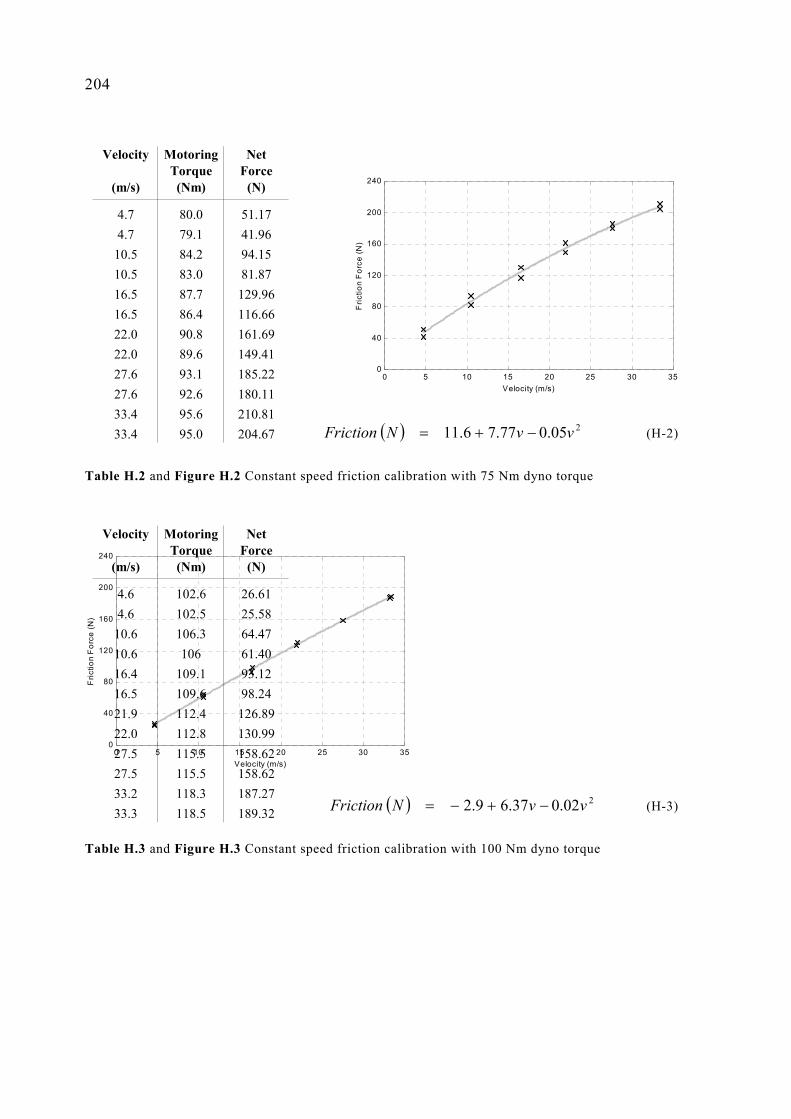
204
0 5 10 15 20 25 30 350
40
80
120
160
200
240
Velocity (m/s)
Fric
tion
For
ce (N
)
( ) 205.077.76.11 vvNFriction −+= (H-2)
Table H.2 and Figure H.2 Constant speed friction calibration with 75 Nm dyno torque
0 5 10 15 20 25 30 350
40
80
120
160
200
240
Velocity (m/s)
Fric
tion
For
ce (N
)
( ) 202.037.69.2 vvNFriction −+−= (H-3)
Table H.3 and Figure H.3 Constant speed friction calibration with 100 Nm dyno torque
Velocity Motoring NetTorque Force
(m/s) (Nm) (N)
4.7 80.0 51.174.7 79.1 41.96
10.5 84.2 94.1510.5 83.0 81.8716.5 87.7 129.9616.5 86.4 116.6622.0 90.8 161.6922.0 89.6 149.4127.6 93.1 185.2227.6 92.6 180.1133.4 95.6 210.8133.4 95.0 204.67
Velocity Motoring NetTorque Force
(m/s) (Nm) (N)
4.6 102.6 26.614.6 102.5 25.58
10.6 106.3 64.4710.6 106 61.4016.4 109.1 93.1216.5 109.6 98.2421.9 112.4 126.8922.0 112.8 130.9927.5 115.5 158.6227.5 115.5 158.6233.2 118.3 187.2733.3 118.5 189.32

APPENDIX H: Constant Speed Friction Determination 205
0 5 10 15 20 25 30 350
40
80
120
160
200
240
Velocity (m/s)
Fric
tion
For
ce (N
)
Figure H.4 Constant speed friction calibration combining all runs
( ) 203.086.628.13 vvNFriction −+= (H-4)


207
APPENDIX I:
Inertia Coastdown Results with an Assumed Friction Force
The following data was gathered in a series of decelerations under constant torque
from both the motor and the power absorber. The chassis dynamometer friction was
assumed to be as follows:
2031.086.627.13 vvFf −+= (I-1)
Where v is in m/s
So that the equivalent mass at any point in time during a coastdown can be found
using Equation 5-1 (see Section 5.2.1).
Table I.1 Results summary table from inertia coastdowns incorporating motor torque and
assumed friction coefficients.
Nominal Average Average Averagedyno torque dyno torque motor torque Run 1 Run 2 Run 3 Run 4 equiv. Mass
(Nm) (Nm) (Nm) (kg) (kg) (kg) (kg) (kg) (kg) (%)
50 51.02 25.32 726.5 730.1 734.3 731.5 730.6 3.2 0.44
75 77.17 25.93 713.7 716.2 717.1 718.7 716.4 2.1 0.29
100 102.53 26.32 709.3 711.7 711.7 715.6 712.1 2.6 0.37
125 128.29 25.76 707.7 707.3 707.2 707.6 707.5 0.2 0.03
Combined Data 716.6 9.2 1.28
Calculated equivalent mass (kg) StandardDeviation


209
APPENDIX J:
Inertia Determination Results using Acceleration/Deceleration Method
The tables below include the complete results of the inertia determination as detailed
in Section 5.2.2. Results are summarised in Table 5.1.
vA = Highest speed during run
vA = Lowest speed during run
Fmotor = Electric motor force, referenced to the drum surface
Fdyno = Power absorber force, referenced to the drum surface
∆t = Time interval for acceleration/deceleration
Table J.1 Acceleration/Deceleration results set A
RESULTS SET A Equivalent Mass, m cd = 696.2 kg
Deceleration 1 2 3 Average
v A (m/s) 16.71 16.66 16.66 16.68v B (m/s) 22.18 22.18 22.13 22.16F motor (N) 256.98 258.00 258.00 257.66F dyno (N) 517.02 517.02 517.02 517.02∆ t (s) 9.90 9.90 9.90 9.90
Acceleration 1 2 3 Average
v A (m/s) 16.66 16.66 16.57 16.63v B (m/s) 22.18 22.18 22.13 22.16F motor (N) 723.83 723.83 723.83 723.83F dyno (N) 208.86 207.83 207.83 208.17∆ t (s) 9.90 9.90 9.90 9.90
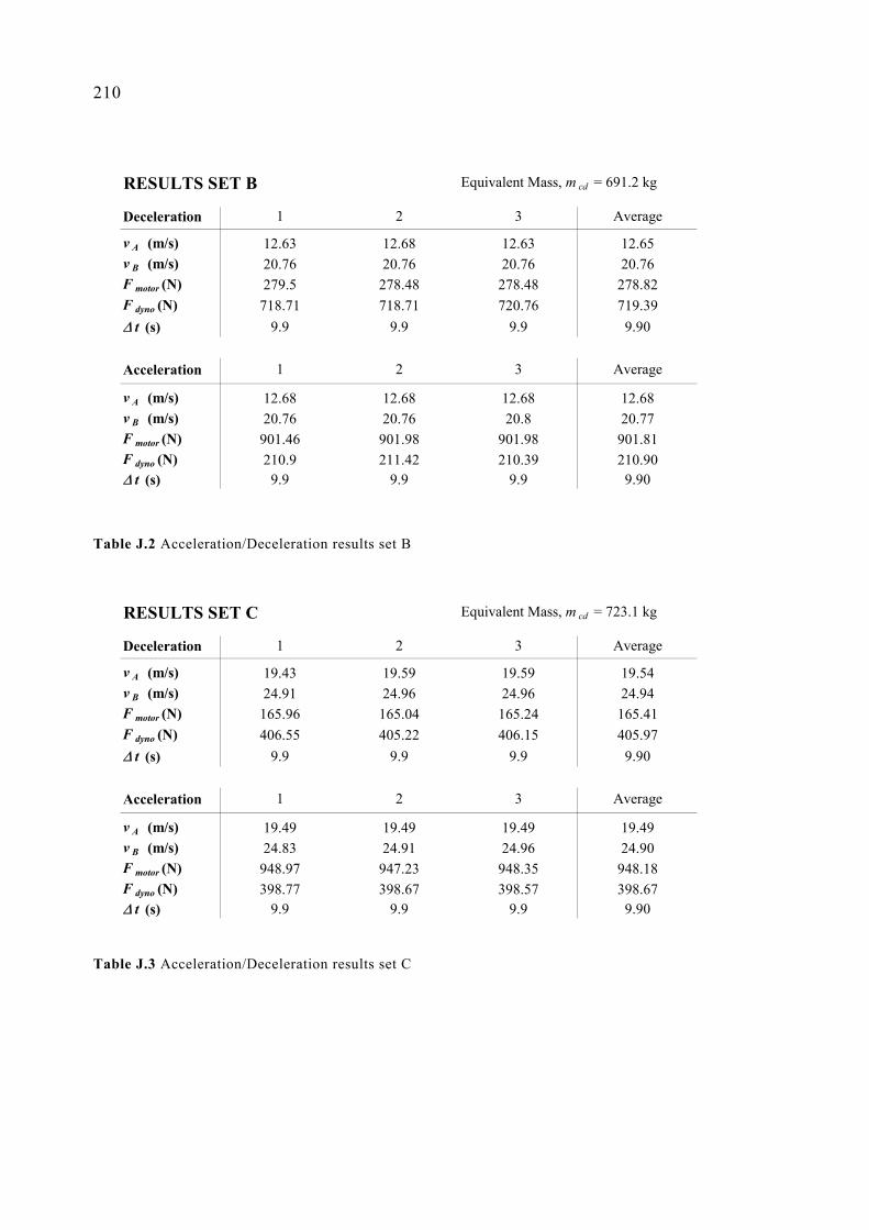
210
Table J.2 Acceleration/Deceleration results set B
Table J.3 Acceleration/Deceleration results set C
RESULTS SET B Equivalent Mass, m cd = 691.2 kg
Deceleration 1 2 3 Average
v A (m/s) 12.63 12.68 12.63 12.65v B (m/s) 20.76 20.76 20.76 20.76F motor (N) 279.5 278.48 278.48 278.82F dyno (N) 718.71 718.71 720.76 719.39∆ t (s) 9.9 9.9 9.9 9.90
Acceleration 1 2 3 Average
v A (m/s) 12.68 12.68 12.68 12.68v B (m/s) 20.76 20.76 20.8 20.77F motor (N) 901.46 901.98 901.98 901.81F dyno (N) 210.9 211.42 210.39 210.90∆ t (s) 9.9 9.9 9.9 9.90
RESULTS SET C Equivalent Mass, m cd = 723.1 kg
Deceleration 1 2 3 Average
v A (m/s) 19.43 19.59 19.59 19.54v B (m/s) 24.91 24.96 24.96 24.94F motor (N) 165.96 165.04 165.24 165.41F dyno (N) 406.55 405.22 406.15 405.97∆ t (s) 9.9 9.9 9.9 9.90
Acceleration 1 2 3 Average
v A (m/s) 19.49 19.49 19.49 19.49v B (m/s) 24.83 24.91 24.96 24.90F motor (N) 948.97 947.23 948.35 948.18F dyno (N) 398.77 398.67 398.57 398.67∆ t (s) 9.9 9.9 9.9 9.90

APPENDIX J: Inertia Determination Results using Acceleration/Deceleration Method 211
Table J.4 Acceleration/Deceleration results set D
Table J.5 Acceleration/Deceleration results set E
RESULTS SET D Equivalent Mass, m cd = 717.5 kg
Deceleration 1 2 3 Average
v A (m/s) 14.37 14.42 14.42 14.40v B (m/s) 19.43 19.43 19.43 19.43F motor (N) 151.83 151.63 150.91 151.46F dyno (N) 382.7 381.47 381.51 381.89∆ t (s) 9.9 9.9 9.9 9.90
Acceleration 1 2 3 Average
v A (m/s) 14.37 14.42 14.37 14.39v B (m/s) 19.43 19.49 19.49 19.47F motor (N) 898.5 898.8 898.39 898.56F dyno (N) 396.32 396.32 396.11 396.25∆ t (s) 9.9 9.9 9.9 9.90
RESULTS SET E Equivalent Mass, m cd = 719.0 kg
Deceleration 1 2 3 Average
v A (m/s) 9.05 9.1 9.1 9.08v B (m/s) 13.86 13.86 13.86 13.86F motor (N) 144.54 144.69 143.7 144.31F dyno (N) 373.69 374.1 373.85 373.88∆ t (s) 9.9 9.9 9.9 9.90
Acceleration 1 2 3 Average
v A (m/s) 9.1 9.1 9.1 9.10v B (m/s) 13.86 13.86 13.86 13.86F motor (N) 866.52 864.12 864.01 864.88F dyno (N) 402.26 401.92 401.2 401.79∆ t (s) 9.9 9.9 9.9 9.90


213
APPENDIX K:
Electric Motor Response with Software Integrator
Figure K.1 below shows the electric motor step response under control from the
existing analogue hardware and an additional software ‘integrator’. The integrator
term (dependent on the control error) was simply added to the D/A output as shown
below:
u(k)pointsetDemanddemandAD +=/ (K-1)
Where:
)u(ke(k)ku 1)01.0()( −−= (K-2)
With: e(k) = Error between set point and current measured torque (Nm)
u(k) = Current integrator output (Nm)
u(k-1) = Integrator output at previous time interval (Nm)
Note that while the 0.01 factor is small, the tiny fluctuations brought about by this
additional control (which includes some lag between the error being read and the
physical application of load) lead to instability in the motor torque. Note also that the
integrator ‘winds up’ during the delay between the step input and the motor response.
This wind-up leads the overshoot seen in Figure K.1.
0 2 4 6 8 10 12 14 16 18 20 22 24
0
10
20
30
40
50
Time (sec)
Torq
ue (N
m)
Controller demand torqueAchieved motor torque
INTEGRATOR WIND-UP
Figure K.1 Step response of electric motor with integrator control software


215
APPENDIX L:
Inertia Coastdown Combined Results
The results of 32 individual chassis dynamometer coastdowns were averaged and
combined to arrive at a single base inertia for the system. Eight coastdowns were
carried out at each of the power absorber torques shown below (see Table L.1) and
the velocity and dynamometer load cell readings were averaged at each recorded
point. Different power absorber torques were used to bring about different rates of
deceleration.
Table L.1 Inertia coastdown runs combined to give four ‘average coastdowns’
The ‘average coastdowns’ at each power absorber load were combined with the
others in each of the possible ways, as shown in Table L.2. The resultant equivalent
mass (in kg) for each pair was also calculated as an average. By simultaneously
solving for equivalent mass (see Equation 5-6 in Section 5.3) at 20 different
velocities in the range 35–105 kph, single mass was found for each combination of
dynamometer torques. For example, the first row in Table L.2 contains the base
masses calculated by simultaneously solving between 40A & 60A, 40A & 80A, and
40A & 100A.
Nominal dyno torque (Nm) 40 60 80 100
Coastdown run number 1 2 3 4
5 6 7 8
9 10 11 12
13 14 15 16
17 18 19 20
21 22 23 24
25 26 27 28
29 30 31 32
Average grouping (see below) 40A 60A 80A 100A

216
Table L.2 Equivalent masses (in kilograms) found by simultaneously solving for each averaged
coastdown pair
The overall average equivalent mass was 673.8 kg, with a standard deviation from
Table L.2 of 2.3 kg (0.34%).
60A 80A 100A
40A 672.1 672.1 674.0
60A 672.1 674.9
80A 677.8

217
APPENDIX M:
Friction Coastdown Repeatability Results
The total friction forces at two different speeds were calculated using the data from
32 separate coastdowns, under several different dynamometer loads. Equation 5-11
(see Section 5.4) may be solved with knowledge of the system inertia, dynamometer
force, and instantaneous acceleration. The latter was differentiated from a quadratic
least squares approximation of velocity throughout each coastdown run. In Table M.1
and Table M.2, the total friction is listed for each individual run, as well as the
average friction found by combining all the coastdown runs at a particular
dynamometer torque. An overall average (for each of the two speeds) was found by
combining the data from all 32 coastdowns.
Table M.1 Friction calibration results at 35 kph for 32 separate coastdowns
Nominal Dyno Torque (Nm) 40 60 80 100 40 60 80 100
Friction force (N) at 35 kph 71.26 72.38 73.71 71.36 74.53 73.92 74.84 73.82for individual coastdowns 72.18 71.87 72.38 71.46 75.66 74.84 74.64 74.33
71.97 72.59 73.10 71.05 73.71 74.02 75.86 74.7471.46 72.28 72.90 70.95 75.86 74.84 74.33 74.23
Average and variation mean (N) 71.72 72.28 73.02 71.21 74.94 74.41 74.92 74.28for each dyno torque s.d. (N) 0.43 0.30 0.55 0.24 1.01 0.50 0.67 0.38
s.d. (%) 0.60 0.42 0.75 0.34 1.34 0.68 0.89 0.51
Average and variation mean (N) 72.06 74.64across all of Results Set s.d. (N) 0.78 0.68
s.d. (%) 1.09 0.91
Average and variation mean (N) 73.35across all data s.d. (N) 1.50
s.d. (%) 2.04
Results Set A Results Set B

218
Table M.2 Friction calibration results at 105 kph for 32 separate coastdowns
Nominal Dyno Torque (Nm) 40 60 80 100 40 60 80 100
Friction force (N) at 105 kph 135.3 135.1 136.3 136.7 136.4 138.0 138.6 136.2for individual coastdowns 136.0 135.5 135.7 133.5 137.7 137.4 136.9 137.0
136.3 134.8 136.3 136.4 136.8 138.5 138.4 135.8136.4 136.4 135.8 134.7 137.1 137.0 136.6 137.1
Average and variation mean (N) 136.0 135.5 136.0 135.3 137.0 137.7 137.6 136.5for each dyno torque s.d. (N) 0.46 0.66 0.33 1.48 0.56 0.68 1.05 0.64
s.d. (%) 0.34 0.49 0.24 1.10 0.41 0.49 0.76 0.47
Average and variation mean (N) 135.7 137.2across all of Results Set s.d. (N) 0.83 0.85
s.d. (%) 0.61 0.62
Average and variation mean (N) 136.45across all data s.d. (N) 1.13
s.d. (%) 0.83
Results Set A Results Set B

219
APPENDIX N:
Drum Inertia Coastdown Combined Results
The results of 32 individual chassis dynamometer coastdowns were averaged and
combined to arrive at a single inertia for the roller drum assembly. Four coastdowns
were carried out at each of the power absorber torques shown below (see Table N.1)
and the velocity and tractive effort load cell readings were averaged at each recorded
point.
Table N.1 Inertia coastdown runs combined to give four ‘average coastdowns’
The ‘average coastdowns’ at each power absorber load were combined with the
others in each of the possible ways, as shown in Table N.2. The resultant equivalent
mass (in kilograms) for each pair was also calculated as an average. Equation 5-14
was used (neglecting the trunnion friction) to determine the roller drum equivalent
mass by simultaneously solving to eliminate the friction term, Fdra. The average
inertia over 20 different velocities in the range 30–100 kph provided a single
equivalent mass for each combination of dynamometer torques.
Nominal dyno torque (Nm) 40 60 80 100
Coastdown run number 1 2 3 4
5 6 7 8
9 10 11 12
13 14 15 16
17 18 19 20
21 22 23 24
25 26 27 28
29 30 31 32
Average grouping (see below) 40A 60A 80A 100A
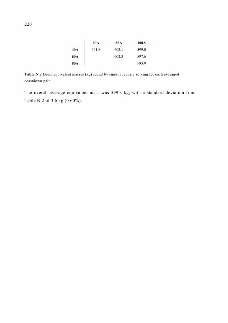
220
Table N.2 Drum equivalent masses (kg) found by simultaneously solving for each averaged
coastdown pair
The overall average equivalent mass was 599.3 kg, with a standard deviation from
Table N.2 of 3.6 kg (0.60%).
60A 80A 100A
40A 601.8 602.1 599.0
60A 602.3 597.6
80A 593.0

221
APPENDIX O:
Drum Friction Coastdown Repeatability Results
The roller drum friction forces at two different speeds were calculated using the data
from 32 separate coastdowns, under several different dynamometer loads (i.e.
different rates of deceleration). Equation 5-14 (see Section 5.5.1) may be solved with
knowledge of the drum inertia, tractive effort load cell force, and instantaneous
acceleration (again, neglecting trunnion friction). The latter was differentiated from a
quadratic least squares approximation of velocity throughout each coastdown run. In
Tables O.1 and O.2, the friction is listed for each individual run, as well as the
average friction found by combining all the coastdown runs at a particular
dynamometer torque. An overall average (for each of the two speeds) was found by
combining the data from all 32 coastdowns.
Table O.1 Drum friction calibration results at 35 kph for 32 separate coastdowns
Nominal Dyno Torque (Nm) 40 60 80 100 40 60 80 100
Friction force (N) at 35 kph 6.87 6.58 5.45 7.21 4.05 3.86 2.30 3.46for individual coastdowns 6.39 6.28 5.37 5.87 2.62 3.57 2.87 3.78
5.49 7.02 4.95 5.86 2.97 3.56 1.84 3.416.01 6.53 5.60 6.09 2.45 3.39 2.37 3.78
Average and variation mean (N) 6.19 6.60 5.34 6.26 3.02 3.59 2.35 3.61for each dyno torque s.d. (N) 0.59 0.31 0.28 0.64 0.72 0.20 0.42 0.20
s.d. (%) 9.5 4.7 5.2 10.3 23.8 5.5 18.0 5.6
Average and variation mean (N) 6.10 3.14across all of Results Set s.d. (N) 0.65 0.66
s.d. (%) 10.6 21.1
Average and variation mean (N) 4.6across all data s.d. (N) 1.6
s.d. (%) 35.4
Results Set A Results Set B

222
Table O.2 Drum friction calibration results at 105 kph for 32 separate coastdowns
Note that the uncertainties represented by the large (as a percentage) standard
deviations are with the estimated measurement uncertainty of the tractive effort load
cell (±9 N, see Appendix C.5).
Nominal Dyno Torque (Nm) 40 60 80 100 40 60 80 100
Friction force (N) at 105 kph 23.8 23.2 24.2 24.4 20.8 20.5 21.0 21.8for individual coastdowns 24.5 23.7 24.0 25.2 22.3 20.0 20.2 22.1
26.0 22.3 23.7 25.2 21.5 20.5 20.9 22.623.8 23.5 22.8 24.5 22.8 20.0 21.0 21.6
Average and variation mean (N) 24.5 23.2 23.7 24.8 21.8 20.2 20.8 22.0for each dyno torque s.d. (N) 1.05 0.64 0.64 0.43 0.87 0.29 0.38 0.43
s.d. (%) 4.3 2.8 2.7 1.7 4.0 1.4 1.8 2.0
Average and variation mean (N) 24.0 21.2across all of Results Set s.d. (N) 0.94 0.91
s.d. (%) 3.9 4.3
Average and variation mean (N) 22.6across all data s.d. (N) 1.7
s.d. (%) 7.5
Results Set A Results Set B

223
APPENDIX P:
C++ Program Menu Structure
Table P.1 Main chassis dynamometer program menu options
Menu Menu Options Sub-Menu Options
Info Program infoVideo modeColours
File OpenViewNewSaveSave asSet config fileSet vehicle fileSet cycle fileEdit vehicle specs New vehicle file
Edit existing fileDOS shellExit
Edit UndoCutCopyPasteShow clipboardClear
Calibrate PCL-812PG A/D card A/D inputsD/A outputs
Friction Constants Dynamometer frictionVehicle + dyno friction
Rezero load cells Dyno load cellTractive effort load cell
Emissions equipment NOx meterTest Program
Run Warm UpRoad load drivingManual controlMapping testDriving cycle
Window Size/moveZoomCascadeTileNextPreviousClose

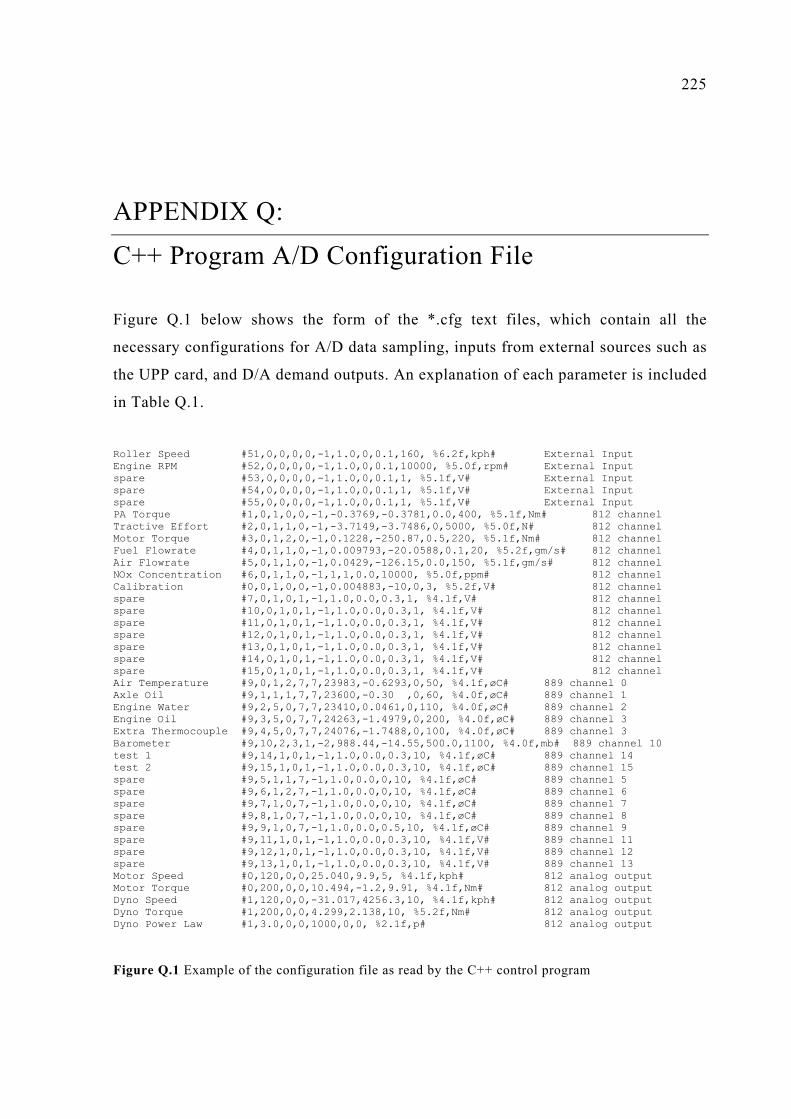
225
APPENDIX Q:
C++ Program A/D Configuration File
Figure Q.1 below shows the form of the *.cfg text files, which contain all the
necessary configurations for A/D data sampling, inputs from external sources such as
the UPP card, and D/A demand outputs. An explanation of each parameter is included
in Table Q.1.
Roller Speed #51,0,0,0,0,-1,1.0,0,0.1,160, %6.2f,kph# External Input Engine RPM #52,0,0,0,0,-1,1.0,0,0.1,10000, %5.0f,rpm# External Input spare #53,0,0,0,0,-1,1.0,0,0.1,1, %5.1f,V# External Input spare #54,0,0,0,0,-1,1.0,0,0.1,1, %5.1f,V# External Input spare #55,0,0,0,0,-1,1.0,0,0.1,1, %5.1f,V# External Input PA Torque #1,0,1,0,0,-1,-0.3769,-0.3781,0.0,400, %5.1f,Nm# 812 channel Tractive Effort #2,0,1,1,0,-1,-3.7149,-3.7486,0,5000, %5.0f,N# 812 channel Motor Torque #3,0,1,2,0,-1,0.1228,-250.87,0.5,220, %5.1f,Nm# 812 channel Fuel Flowrate #4,0,1,1,0,-1,0.009793,-20.0588,0.1,20, %5.2f,gm/s# 812 channel Air Flowrate #5,0,1,1,0,-1,0.0429,-126.15,0.0,150, %5.1f,gm/s# 812 channel NOx Concentration #6,0,1,1,0,-1,1,1,0.0,10000, %5.0f,ppm# 812 channel Calibration #0,0,1,0,0,-1,0.004883,-10,0,3, %5.2f,V# 812 channel spare #7,0,1,0,1,-1,1.0,0.0,0.3,1, %4.1f,V# 812 channel spare #10,0,1,0,1,-1,1.0,0.0,0.3,1, %4.1f,V# 812 channel spare #11,0,1,0,1,-1,1.0,0.0,0.3,1, %4.1f,V# 812 channel spare #12,0,1,0,1,-1,1.0,0.0,0.3,1, %4.1f,V# 812 channel spare #13,0,1,0,1,-1,1.0,0.0,0.3,1, %4.1f,V# 812 channel spare #14,0,1,0,1,-1,1.0,0.0,0.3,1, %4.1f,V# 812 channel spare #15,0,1,0,1,-1,1.0,0.0,0.3,1, %4.1f,V# 812 channel Air Temperature #9,0,1,2,7,7,23983,-0.6293,0,50, %4.1f,øC# 889 channel 0 Axle Oil #9,1,1,1,7,7,23600,-0.30 ,0,60, %4.0f,øC# 889 channel 1 Engine Water #9,2,5,0,7,7,23410,0.0461,0,110, %4.0f,øC# 889 channel 2 Engine Oil #9,3,5,0,7,7,24263,-1.4979,0,200, %4.0f,øC# 889 channel 3 Extra Thermocouple #9,4,5,0,7,7,24076,-1.7488,0,100, %4.0f,øC# 889 channel 3 Barometer #9,10,2,3,1,-2,988.44,-14.55,500.0,1100, %4.0f,mb# 889 channel 10 test 1 #9,14,1,0,1,-1,1.0,0.0,0.3,10, %4.1f,øC# 889 channel 14 test 2 #9,15,1,0,1,-1,1.0,0.0,0.3,10, %4.1f,øC# 889 channel 15 spare #9,5,1,1,7,-1,1.0,0.0,0,10, %4.1f,øC# 889 channel 5 spare #9,6,1,2,7,-1,1.0,0.0,0,10, %4.1f,øC# 889 channel 6 spare #9,7,1,0,7,-1,1.0,0.0,0,10, %4.1f,øC# 889 channel 7 spare #9,8,1,0,7,-1,1.0,0.0,0,10, %4.1f,øC# 889 channel 8 spare #9,9,1,0,7,-1,1.0,0.0,0.5,10, %4.1f,øC# 889 channel 9 spare #9,11,1,0,1,-1,1.0,0.0,0.3,10, %4.1f,V# 889 channel 11 spare #9,12,1,0,1,-1,1.0,0.0,0.3,10, %4.1f,V# 889 channel 12 spare #9,13,1,0,1,-1,1.0,0.0,0.3,10, %4.1f,V# 889 channel 13 Motor Speed #0,120,0,0,25.040,9.9,5, %4.1f,kph# 812 analog output Motor Torque #0,200,0,0,10.494,-1.2,9.91, %4.1f,Nm# 812 analog output Dyno Speed #1,120,0,0,-31.017,4256.3,10, %4.1f,kph# 812 analog output Dyno Torque #1,200,0,0,4.299,2.138,10, %5.2f,Nm# 812 analog output Dyno Power Law #1,3.0,0,0,1000,0,0, %2.1f,p# 812 analog output
Figure Q.1 Example of the configuration file as read by the C++ control program
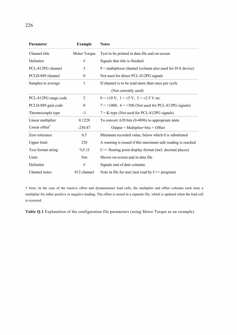
226
† Note: In the case of the tractive effort and dynamometer load cells, the multiplier and offset columns each store a
multiplier for either positive or negative loading. The offset is stored in a separate file, which is updated when the load cell
is rezeroed.
Table Q.1 Explanation of the configuration file parameters (using Motor Torque as an example)
Parameter Example Notes
Channel title Motor Torque Text to be printed in data file and on-screen
Delimiter # Signals that title is finished
PCL-812PG channel 3 9 = multiplexer channel (column also used for D/A device)
PCLD-889 channel 0 Not used for direct PCL-812PG signals
Samples to average 1 If channel is to be read more than once per cycle
(Not currently used)
PCL-812PG range code 2 0 = ±10 V, 1 = ±5 V, 2 = ±2.5 V etc
PCLD-889 gain code 0 7 = ×1000, 6 = ×500 (Not used for PCL-812PG signals)
Thermocouple type -1 7 = K-type (Not used for PCL-812PG signals)
Linear multiplier 0.1228 To convert A/D bits (0-4096) to appropriate units
Linear offset† -250.87 Output = Multiplier×bits + Offset
Zero tolerance 0.5 Minimum recorded value, below which 0 is substituted
Upper limit 220 A warning is issued if this maximum safe reading is reached
Text format string %5.1f C++ floating point display format (incl. decimal places)
Units Nm Shown on-screen and in data file
Delimiter # Signals end of data columns
Channel notes 812 channel Note in file for user (not read by C++ program)

227
APPENDIX R:
Example of C++ Program Data File Output
Figure R.1 on the following page shows part of a text file saved using the C++ data
acquisition and control program.

228
Figure R.1 Example data-file output from C++ data acquisition program
***************************************************************** New Session with configuration: Config File: C:\CHASSIS\D_TEST.CFG, Car File: C:\CHASSIS\CARS\CELICA.CAR Dyno Offsets: NORMAL: 770.3 REVERSE: 776.2, Drum Offsets: ZERO: 2046.4 PLUS: 7602.4 MINUS: 7671.3 Friction Coefficents: SYSTEM: 3.61, 0.328, -0.0006 DRUM/AXLE: 0.00, 0.916, -0.0017 Measured parameters as follows: Count (), Time (sec), Delay (%), Accel. (m/sý), Raw T.E. (N), Power (W), Roller Speed (kph), Engine RPM (rpm), PA Torque (Nm), Tractive Effort (N), Motor Torque (Nm), Fuel Flowrate (gm/s), Air Flowrate (gm/s), NOx Concentration (ppm), Air Temperature (øC), Axle Oil (øC), Engine Water (øC), Engine Oil (øC), Extra Thermocouple (øC), Barometer (mb), ASEA Demand (), Froude Demand (), Motor Start/Auto/Mode (), Dyno Run/Auto/Mode () ================================================================= 1.) Timed Sequence No.1 Date/time = Mon Nov 12 16:40:04 2001 ================================================================= 0, 0.0, 5, 2.187, 1554.75, 25.00, 31.30, 2122, 1.0, 2873, 4.8, 1.72, 14.2, ...., ...., more channels,....... 1, 0.1, 42, 2.205, 1575.18, 26.46, 32.77, 2232, 1.1, 2904, 4.8, 1.85, 15.4, ...., ...., more channels,....... 2, 0.2, 42, 2.200, 1591.65, 27.93, 34.43, 2270, 1.1, 2918, 4.8, 1.98, 16.6, ...., ...., etc 3, 0.3, 42, 2.190, 1583.97, 28.99, 35.90, 2478, 1.1, 2905, 4.8, 2.06, 17.6, ...., ...., 4, 0.4, 42, 2.137, 1588.18, 29.90, 37.37, 2492, 1.1, 2877, 4.8, 2.17, 18.9, ...., 5, 0.5, 41, 2.130, 1593.75, 31.25, 39.03, 2621, 1.2, 2879, 4.8, 2.25, 20.2, ... 6, 0.6, 42, 2.164, 1584.96, 32.64, 40.60, 2712, 1.4, 2891, 4.8, 2.37, 21.4, ... 7, 0.7, 42, 2.158, 1577.28, 33.69, 42.07, 2825, 1.5, 2880, 4.8, 2.44, 22.5, .. 8, 0.8, 42, 2.117, 1576.79, 34.58, 43.54, 2948, 1.5, 2856, 4.8, 2.57, 23.8, .. 9, 0.9, 42, 2.078, 1580.50, 35.50, 45.02, 3042, 1.5, 2837, 4.8, 2.70, 25.1, .. 10, 1.0, 42, 2.070, 1571.41, 36.80, 47.10, 3172, 1.2, 2837, 4.8, 2.81, 26.3, .. ================================================================ 2.) Timed Sequence No.2 Date/time = Mon Nov 12 16:45:32 2001 ================================================================= 0, 0.0, 6, 2.171, 1621.37, 41.99, 51.46, 3437, 1.8, 2935, 4.8, 3.17, 30.8, ...., ... 1, 0.1, 42, 2.201, 1636.23, 43.68, 52.93, 3585, 1.8, 2968, 4.8, 3.32, 32.2, ...., ... 2, 0.2, 42, 2.203, 1648.24, 45.25, 54.59, 3651, 1.9, 2981, 4.8, 3.42, 33.8, ...., ... 3, 0.3, 42, 2.237, 1651.09, 46.99, 56.25, 3731, 2.1, 3005, 4.8, 3.58, 35.4, ... 4, 0.4, 42, 2.249, 1669.66, 48.73, 57.81, 3872, 2.2, 3031, 4.7, 3.74, 36.9, .. 5, 0.5, 42, 2.250, 1677.09, 50.26, 59.47, 3978, 2.2, 3039, 4.7, 3.89, 38.4, . 6, 0.6, 41, 2.224, 1674.49, 51.20, 60.94, 4142, 2.2, 3022, 4.7, 4.05, 39.8, 7, 0.7, 42, 2.219, 1673.38, 52.60, 62.69, 4206, 2.2, 3018, 4.7, 4.17, 41.1, 8, 0.8, 42, 2.224, 1662.23, 53.69, 64.16, 4315, 2.4, 3010, 4.7, 4.27, 42.6, 9, 0.9, 42, 2.208, 1646.75, 54.64, 65.82, 4428, 2.6, 2986, 4.7, 4.41, 44.1, 10, 1.0, 42, 2.191, 1632.51, 55.40, 67.29, 4532, 2.6, 2961, 4.7, 4.54, 45.8,
Figure R.1 Example data-file output from C++ data acquisition program
NEW SESSION DIVIDER A/D CONFIGURATION FILE VEHICLE
DATA FILE LOAD CELL AND FRICTION DATA
12th CHANNEL TITLE MATCHES 12th DATA COLUMN
2nd CHANNEL TITLE MATCHES 2nd
DATA COLUMN
NEW RUNS EACH HAVE SETTINGS AND CHANNELS
AS PER THE SESSION HEADER

229
APPENDIX S:
Chassis Dynamometer Friction Coastdown Raw Data
0 5 10 15 20 25 30 355
10
15
20
25
30
Time (sec)
Vel
ocity
(m/s
)
Figure S.1 Raw velocity measured during chassis dynamometer friction coastdown
0 5 10 15 20 25 30 35-0.61
-0.6
-0.59
-0.58
-0.57
-0.56
-0.55
-0.54
-0.53
-0.52
Time (sec)
Leas
t squ
ares
acc
eler
atio
n (m
/s2 )
Figure S.2 Coastdown acceleration calculated from least squares approximation of velocity

230
0 5 10 15 20 25 30 3548.5
48.75
49
49.25
49.5
49.75
50
50.25
50.5
Time (sec)
Pow
er a
bsor
ber t
orqu
e (N
m)
Power absorber torque linear fit Raw power absorber load cell reading
Figure S.3 Coastdown power absorber torque raw data and least squares linear approximation
0 5 10 15 20 25 30 35
225
230
235
240
245
250
Time (sec)
Trac
tive
effo
rt lo
ad c
ell f
orce
(N)
Tractive effort linear fit Raw tractive effort reading
Figure S.4 Coastdown tractive force raw data and least squares linear approximation

231
APPENDIX T:
Dynamometer Warm Up Procedure
To stabilise the frictional characteristics of the shaft bearings and differential, the
dynamometer was rotated under power from the electric motor. The necessary speed
and duration of this warming up period was determined in several tests, using friction
coastdowns (see Section 5.4) to calculate the overall system friction at a certain
speed (35 kph for Figures T.1 and T.2 below). The time periods labelled with letters
indicate intervals of constant speed running, while each data point is the result of a
single coastdown.
Table T.1 Warm up activities indicated in Figure T.1
Note that interval C includes more than one constant velocity phase.
0 5 10 15 20 25 30 35 40 45 50 55 60
7.2
7.4
7.6
7.8
8
8.2
8.4
Time (min)
Cal
cula
ted
frict
ion
forc
e at
35k
ph (N
)
A C B
Figure T.1 First warm up test results showing frictional force referenced to the drum surface
Interval Velocity (kph) Duration (min)
A 60 15
B 60 15
C 120 350 1

232
Figure T.1 shows that 30 minutes at 60 kph (intervals A and B) was insufficient to
reach a stable frictional state. As the coastdowns were performed between intervals B
and C, the raising of the dynamometer speed to approximately 120 kph for the start
of each run continued to raise the temperature—and hence, lower the friction—in the
bearings and differential gears. A more stable state was achieved after brief running
at 120 kph (interval C), as shown by the flattening trend in the calculated friction.
Table T.2 Warm up activities indicated in Figure T.2
Note that all warm up procedures were carried out before the series of friction
coastdowns.
0 5 10 15 20 25 30 35 40 45 50
6.2
6.4
6.6
6.8
7
7.2
7.4
Time (min)
Cal
cula
ted
frict
ion
forc
e at
35k
ph (N
)
A B
Figure T.2 Second warm-up test results showing frictional force referenced to the drum surface
After the initial warming up, the system friction increased with subsequent
coastdowns, although less than the decrease shown in Figure T.1. This suggests that
the contacting elements were cooling down, and that the frictional forces
immediately after the warm up period were less than the equilibrium reached during
consecutive friction coastdowns. In fact, once the drum axle oil reaches its desired
temperature range (≈50ºC controlled by a heat exchanger), the equilibrium friction
Interval Velocity (kph) Duration (min)
A 60 15
B 80 1100 1120 8
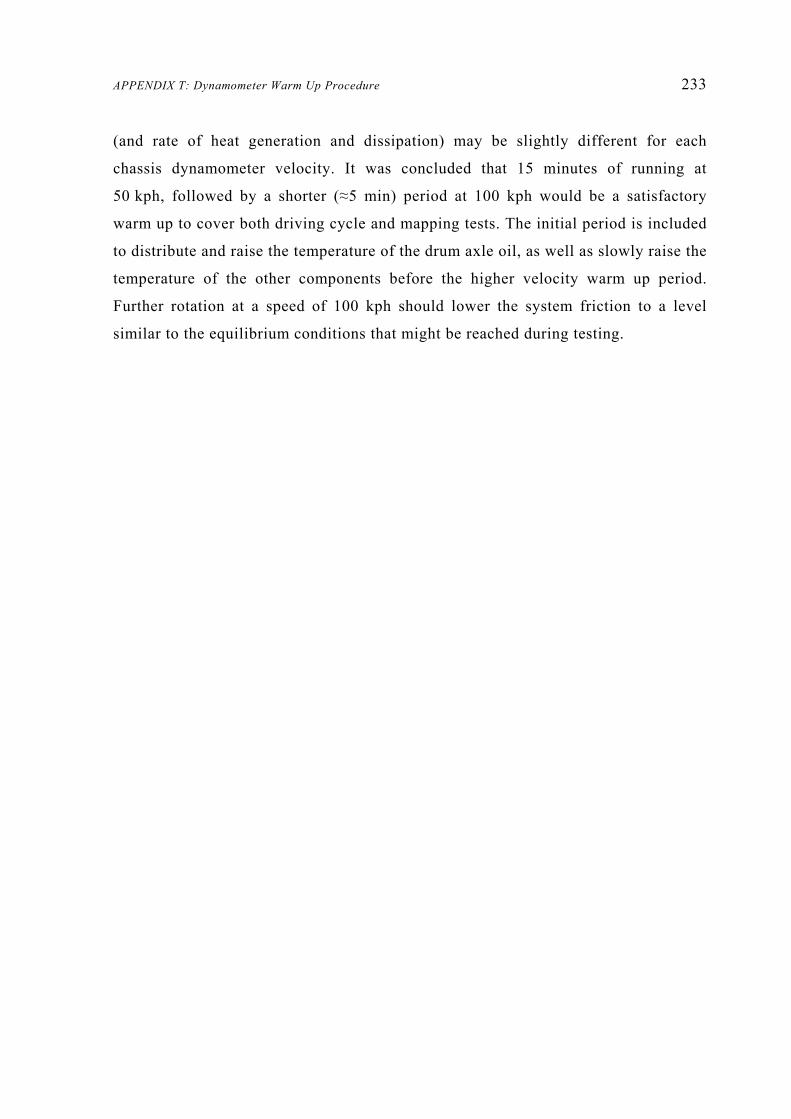
APPENDIX T: Dynamometer Warm Up Procedure 233
(and rate of heat generation and dissipation) may be slightly different for each
chassis dynamometer velocity. It was concluded that 15 minutes of running at
50 kph, followed by a shorter (≈5 min) period at 100 kph would be a satisfactory
warm up to cover both driving cycle and mapping tests. The initial period is included
to distribute and raise the temperature of the drum axle oil, as well as slowly raise the
temperature of the other components before the higher velocity warm up period.
Further rotation at a speed of 100 kph should lower the system friction to a level
similar to the equilibrium conditions that might be reached during testing.


235
APPENDIX U:
Selected Driving Cycles
With the exception of Figure U.1, the following driving cycles are those specified in
SAE J1506 [2001]. Driving cycle files are also included on the accompanying CD.
0 50 100 150 200 250 300 350 400
0
10
20
30
40
50
Time (sec)
Spe
ed (k
ph)
Distance = 2.0km Average speed = 18.3kph
Figure U.1 Driving cycle used for testing at University of Canterbury
0 100 200 300 400 500 600 700 800
0
10
20
30
40
50
Time (sec)
Spe
ed (k
ph)
Average speed = 18.7kph Distance = 4.1km
Figure U.2 Economic Commission for Europe (ECE) R15.04 Schedule

236
0 200 400 600 800 1000 1200 1400
0
20
40
60
80
100
Time (sec)
Spe
ed (k
ph)
Distance = 12.1km Average speed = 31.5kph
Figure U.3 EPA Urban Dynamometer Driving Schedule (UDDS)
0 100 200 300 400 500 600 700 800
0
20
40
60
80
100
Time (sec)
Spe
ed (k
ph)
Average speed = 78.2kph Distance = 16.4km
Figure U.4 Highway Fuel Economy Test Schedule (HWFET)

APPENDIX U: Selected Driving Cycles 237
0 20 40 60 80 100 120 140
0
5
10
15
20
25
30
35
40
Time (sec)
Spe
ed (k
ph)
Average speed = 18.0kph Distance = 0.66km
Figure U.5 Japanese 10-Mode Test Schedule
0 20 40 60 80 100 120
0
10
20
30
40
50
60
Time (sec)
Spe
ed (k
ph)
Average speed = 30.6kph Distance = 1.02km
Figure U.6 Japanese 11-mode Test Schedule


239
APPENDIX V:
NZS 5420:1980 Dynamometer Driving Cycle Tolerance
Figure V.1 Explanatory diagram for clarification of combined speed and time limits (Fig. 2 in New
Zealand Standard NZS 5420 (withdrawn) [1980]


241
APPENDIX W:
MATLAB Program Menu Structure
Table W.1 Menu structure of MATLAB post-processing program
Main Menu Sub-Menu Sub-Menu Options
Choose new data file Select a fileChange extensionChange directoryReturn to Main Menu
Plot data Change x and y variablesChange plot optionsCustomise legendExecute plotPlot power/torque curveVehicle mapping menu Change z and x variables
NEW or REFRESHLevel of interpolationDefault optionsLimit optionsExecute plotExit mapping menu
Exit plot menu
Edit raw data
Calculate additional data Set fuel specificationsCalculate additional dataCalculate drive cycle excursionsExit calculation menu
Exit program


243
APPENDIX X:
Files for Excel Plotting of Vehicle Mapping Data
Each time a vehicle mapping test is plotted using the MATLAB routine detailed in
Section 7.1.3.2, a raw data file (Figure X.1) and a zero-padded grid file are produced.
The text plots (as per Figure 7.8) are generated using the spreadsheet shown in
Figure X.2, with an Excel macro, which retrieves the latest data from the zero-padded
grid file (similar to the grid shown on the left of Figure X.2) for plotting. A copy of
this spreadsheet is also included on the accompanying compact disc.
Velocity Tractive_Force Fuel_Flowrate (kph) (N) (gm/s) ========= ================ ================ 17.1776 1955.9740 0.8430 17.3249 1840.3660 0.7745 17.2329 1605.8215 0.6648 17.2513 1406.6702 0.6084 17.2513 1203.2051 0.5408 17.3065 1008.1865 0.4813 17.2513 795.9034 0.4205 17.3249 607.4649 0.3638 17.3802 400.8932 0.3087 27.4695 2085.3600 1.4567 27.2670 1971.2994 1.2247 27.2670 1811.6699 1.1160 27.2117 1597.7152 1.0184 27.1749 1406.3145 0.9313 28.4085 1197.7678 0.8770 28.2612 998.8357 0.7633 27.8377 807.1908 0.5913 27.8930 590.3657 0.5482 27.9298 406.2272 0.4728
Figure X.1 Partial copy of raw mapping data file

244
Figure X.2 Excel spreadsheet used to create vehicle map text plots
Fuel Flowrate (gm/s) mapData file: c:\Chassis\Save\HH2.DAT
2300
2200 2.759
3.884 4.461 1.835
2100 2.732 1.457 3.223
2.336 4.899
2000 2.649 3.048 3.666 4.806 1.225 4.097
0.843 1.670
1900
0.775
1800 1.116 1.510 2.110 2.386 2.885 3.382 3.836 4.423
1700
1600 0.665 1.018 1.405 1.931 2.200 2.590 3.098 4.079 3.562
1500
1400 0.608 0.931 1.267 1.773 2.065 2.214 2.963 3.317 3.760
1300
1200 0.541 0.877 1.656 1.831 2.674 2.963 3.447 1.166 2.142
1100
2.382 1000 0.481 0.763 1.057 1.428 1.642 1.889 2.647 3.227
900
0.938 800 0.421 0.591 1.232 1.485 1.701 2.061 2.342 2.830
700
1.027 600 0.364 0.548 0.777 1.260 1.514 2.056
1.776 2.565
500
400 0.309 0.473 0.666 0.764 1.063 1.330 1.439 1.777 2.335
300
200
100
017 28 39 51 58 69 80 89 100
Roller Speed (kph)
Trac
tive
Effo
rt (N
)
RUN MACRO "INSERT_DATA" [CTRL-i] TO GET LATEST DATA FROM C:\CHASSIS\TEXTMAP.TXT
2300 0 0 0 0 0 0 0 0 0 0 0 00 0 0 0 0 0 0 0 0 0 0 00 0 0 0 0 0 0 0 0 0 0 00 0 0 0 0 0 0 0 0 0 0 0
2200 0 0 0 0 2.759087 0 0 0 0 0 0 00 0 0 0 0 0 0 0 0 0 0 00 0 0 0 0 0 0 3.883812 4.460522 0 0 00 0 0 1.835116 0 0 0 0 0 0 0 0
2100 0 0 0 0 0 2.731861 0 0 0 0 0 00 0 1.456715 0 0 0 3.222784 0 0 0 0 00 0 0 0 2.336029 0 0 0 0 0 0 00 0 0 0 0 0 0 0 0 4.899346 0 0
2000 0 0 0 0 0 2.649208 3.048273 3.666016 0 4.805529 0 00 0 1.224719 0 0 0 0 0 4.097398 0 0 00 0.842987 0 1.6703 0 0 0 0 0 0 0 00 0 0 0 0 0 0 0 0 0 0 0
1900 0 0 0 0 0 0 0 0 0 0 0 00 0 0 0 0 0 0 0 0 0 0 00 0.774535 0 0 0 0 0 0 0 0 0 00 0 0 0 0 0 0 0 0 0 0 0
1800 0 0 1.116016 1.509891 2.109908 2.386169 2.885415 3.382019 3.835728 4.423112 0 00 0 0 0 0 0 0 0 0 0 0 00 0 0 0 0 0 0 0 0 0 0 00 0 0 0 0 0 0 0 0 0 0 0
1700 0 0 0 0 0 0 0 0 0 0 0 00 0 0 0 0 0 0 0 0 0 0 00 0 0 0 0 0 0 0 0 0 0 00 0 0 0 0 0 0 0 0 0 0 0
1600 0 0.664755 1.01838 1.405008 1.9305 2.200101 2.590157 3.098218 0 4.079182 0 00 0 0 0 0 0 0 0 3.561622 0 0 00 0 0 0 0 0 0 0 0 0 0 00 0 0 0 0 0 0 0 0 0 0 0
1500 0 0 0 0 0 0 0 0 0 0 0 00 0 0 0 0 0 0 0 0 0 0 00 0 0 0 0 0 0 0 0 0 0 00 0 0 0 0 0 0 0 0 0 0 0
1400 0 0.608445 0.93132 1.266535 1.772833 2.06535 2.214301 2.963172 3.317189 3.759833 0 00 0 0 0 0 0 0 0 0 0 0 00 0 0 0 0 0 0 0 0 0 0 00 0 0 0 0 0 0 0 0 0 0 0
1300 0 0 0 0 0 0 0 0 0 0 0 00 0 0 0 0 0 0 0 0 0 0 00 0 0 0 0 0 0 0 0 0 0 00 0 0 0 0 0 0 0 0 0 0 0
1200 0 0.540776 0.876969 0 1.656003 1.831003 0 2.673887 2.963074 3.44724 0 00 0 0 1.166059 0 0 2.141833 0 0 0 0 00 0 0 0 0 0 0 0 0 0 0 00 0 0 0 0 0 0 0 0 0 0 0
1100 0 0 0 0 0 0 0 0 0 0 0 00 0 0 0 0 0 0 0 0 0 0 00 0 0 0 0 0 0 0 0 0 0 00 0 0 0 0 0 0 2.38186 0 0 0 0
1000 0 0.481332 0.763272 1.05716 1.428413 1.641705 1.888586 0 2.646663 3.226702 0 00 0 0 0 0 0 0 0 0 0 0 00 0 0 0 0 0 0 0 0 0 0 00 0 0 0 0 0 0 0 0 0 0 0
900 0 0 0 0 0 0 0 0 0 0 0 00 0 0 0 0 0 0 0 0 0 0 00 0 0 0 0 0 0 0 0 0 0 00 0 0 0.937686 0 0 0 0 0 0 0 0
800 0 0.420518 0.591307 0 1.231574 1.484723 1.700854 2.060649 2.341904 2.830281 0 00 0 0 0 0 0 0 0 0 0 0 00 0 0 0 0 0 0 0 0 0 0 00 0 0 0 0 0 0 0 0 0 0 0
700 0 0 0 0 0 0 0 0 0 0 0 00 0 0 0 0 0 0 0 0 0 0 00 0 0 0 0 0 0 0 0 0 0 00 0 0 0 1.026704 0 0 0 0 0 0 0
600 0 0.363816 0.548218 0.776982 0 1.260267 1.514102 0 2.055557 0 0 00 0 0 0 0 0 0 1.775869 0 2.564891 0 00 0 0 0 0 0 0 0 0 0 0 00 0 0 0 0 0 0 0 0 0 0 0
500 0 0 0 0 0 0 0 0 0 0 0 00 0 0 0 0 0 0 0 0 0 0 00 0 0 0 0 0 0 0 0 0 0 00 0 0 0 0 0 0 0 0 0 0 0
400 0 0.308682 0.472812 0.666224 0.763958 1.062547 1.330483 1.438598 1.77724 2.334755 0 00 0 0 0 0 0 0 0 0 0 0 00 0 0 0 0 0 0 0 0 0 0 00 0 0 0 0 0 0 0 0 0 0 0
300 0 0 0 0 0 0 0 0 0 0 0 00 0 0 0 0 0 0 0 0 0 0 00 0 0 0 0 0 0 0 0 0 0 00 0 0 0 0 0 0 0 0 0 0 0
200 0 0 0 0 0 0 0 0 0 0 0 00 0 0 0 0 0 0 0 0 0 0 00 0 0 0 0 0 0 0 0 0 0 00 0 0 0 0 0 0 0 0 0 0 0
100 0 0 0 0 0 0 0 0 0 0 0 00 0 0 0 0 0 0 0 0 0 0 00 0 0 0 0 0 0 0 0 0 0 00 0 0 0 0 0 0 0 0 0 0 0
0 0 0 0 0 0 0 0 0 0 0 0 00 17.27788 27.672026 39.086969 50.66577 58.488684 68.692161 79.976389 89.45263 99.553016 0 0
x Roller Speed (kph)y Tractive Effort (N)z Fuel Flowrate (gm/s)fi le c:\Chassis\Save\HH2.DAT

245
APPENDIX Y:
Example Vehicle Data Sheet
Table Y.1 Example vehicle data sheet
Vehicle Data Sheet
Type of Vehicle (car/bus/truck) Car
Make/Model Toyota Celica
Year 1982
Owner University of Canterbury
Registration PL 3859
Engine Type/Size 1G-E 6cyl. 2000cc
Initial Odometer Reading (km) 206110
Accessories (if any) -
Unladen mass (kg) 1150
Reference Mass (unladen+100kg) 1250
Dynamometer Equivalent Mass (kg) 1234
Transmission Type 5 spd manual
Axle Ratio unknown
Tyre Make Firestone
Tyre Model/Size F-570 P195/70 R14
Tyre Pressures (kPa) Front 190 Rear 190
Average Tyre Tread (mm) RF:3 LF:4 RR:4 LR:5
Tyre Scrub (mm/metre) Front 2 (inward) Rear 0
Fuel Pump Standard
Carburettor/EFI EFI
Ignition Make/Type Nippondenso
NOTES:


247
APPENDIX Z:
Vehicle Coastdown Friction Calculations
Z.1 On-Road Coastdown Tests
Friction coefficients for the test vehicle were determined experimentally based on the
method prescribed by the SAE Recommended Practice, SAE J1263 [1999].
Several coastdowns between the speeds of 120 kph and 40 kph were carried out on a
section of Tram Road, near Ohoka, Canterbury in both directions. The vehicle
velocity was measured by timing driveshaft rotations using the optical device
mentioned in Section 8.1.1. Initially, the relationship between driveshaft rotations
and displacement of the vehicle was investigated by rolling the vehicle slowly
forward a set number of driveshaft rotations, and measuring the distance travelled.
Table Z.1 Test vehicle distance per driveshaft rotation calibration
Raw velocity vs. time data was approximated by a least squares curve fit, so that the
deceleration at each point could be calculated. With knowledge of the vehicle
deceleration and mass, the frictional force resisting motion is given by:
2210 vfvff
dtdvm VVVVeq ++= (Z-1)
Where: mVeq = Equivalent mass of vehicle including rotational masses
f0V, f1V, f2V = Vehicle frictional coefficients
Driveshaft Distance Metres perrotations (m) rotation
25 12.20 0.488
60 29.21 0.487
60 29.23 0.487
0.487

248
The equivalent mass of the rotating inertias is added to the vehicle mass, and is
approximated as 0.035×(vehicle mass). The three unknowns (f0V, f1V, f2V) may be
solved for simultaneously by calculating mVeq(dv/dt) at several points on the same
coastdown curve.
Of the eight coastdown runs measured, three were discarded, either because an
insufficient maximum speed was achieved before beginning the deceleration, or
because of excessive wind gusts. Ideal coastdown conditions include a perfectly flat
road and zero wind. However, a measurable wind was present (this can be corrected
for, as below), and the calculated coefficients indicated a significant road gradient.
The resulting frictional coefficients do not necessarily comply with the acceptability
criteria detailed in SAE J1263, but were deemed sufficiently accurate for the chassis
dynamometer proving tests in Chapter 8.
Highlight = discarded runs
Table Z.2 Vehicle friction coastdown data
Note that the coefficients are stated such that v in Equation Z-1 is in kilometres per
hour, and friction force is in Newtons. Also, the air temperature and wind velocity
were recorded only at the beginning of runs 1 and 5, and after run 8, with the
remainder of the data linearly interpolated.
Run Temperature Wind f 0V f 1V f 2V
(K) (m/s)
1 295.7 2.20 161.63 0.008 0.0331
2 296.2 -1.65 266.85 0.455 0.0274
3 296.8 1.10 -2.65 4.173 0.0057
4 297.4 -0.55 387.80 -2.355 0.0453
5 298.0 0.00 13.04 3.949 0.0058
6 298.3 -0.40 301.84 -0.465 0.0314
7 298.6 0.80 151.69 0.095 0.0302
8 299.0 -1.20 307.46 -0.875 0.0348

APPENDIX Z: Vehicle Coastdown Friction Calculations 249
Z.2 Correction of Friction Coefficients
Corrections can be made to these coefficients to allow for wind, air temperature, and
air pressure—all of which may affect the frictional resistance to the vehicle’s motion.
Firstly, the rolling resistance is separated from the wind effects to provide a wind
correction to f0V:
2
2220
0 121
x
yDYxVV
v
AvCvffW
µ
ρµ
′−
−−
= (Z-2)
Where: W0µ = is used in Equation Z-3, below
ρ = Mass density of ambient air (kg/m3)
µ ′ = Velocity coefficient of rolling resistance
CDY = Crosswind aerodynamic drag coefficient
vx = Component of wind parallel to track (kph)
vy = Component of wind perpendicular to track (kph)
When exact vehicle data is not available:
µ ′ = 19×10-6 (kph)-2
CDY = 0.8181 (m/s)2/(kph)2
The temperature dependence of the rolling resistance is corrected thus:
( )[ ]000 1 TTkWf tV −+=′ µ (Z-3)
Where: T = Ambient air temperature (K)
T0 = Standard temperature (293.15 K)
kt = 8.6×10⁻³ /ºC unless specific vehicle data is available

250
The coefficient of the v2 term is then adjusted to the standard atmospheric conditions:
( )[ ] VVV fWfpT
Tpf 002
0
02 ′′+′−
=′ µµµ (Z-4)
Where: p = Barometric pressure (mmHg)
p0 = 736.6 mmHg
The linear multiplier, f1V is small and the SAE recommended practice approximates
this factor as zero. However, f1V was maintained for the current work so that its effect
could be investigated.
Z.3 Sample Friction Coefficient Calculations
Run 1 (see Table Z.2) has been included as an example of these correction
calculations. Equation Z-2 becomes:
( ) ( )
( )83.120
379.31
163.765.117.121379.3033.06.161
2
22
0 =′−
×××−×−
=µ
µDYC
W
Where: ( ) ( ) kphwindofanglev x 379.36.32.2cos =××=
( ) ( ) kphwindofanglev y 163.76.32.2sin =××=
316811515927295
743151592
mkgT
pressureair /....
=×
=×
=ρ
=A Frontal area of vehicle, determined using a planimeter on an
elevational photograph (see Plate Z.1).

APPENDIX Z: Vehicle Coastdown Friction Calculations 251
Plate Z.1 Elevational photograph of test vehicle for frontal area determination
The corrected f0V is found using Equation Z-3:
( )[ ] 4312316293662951831200 .... =−+×=′ tV kf
And f2V becomes:
( )[ ] 43123831200330152930743662956736
2 .......
×′+′−
××
=′ µµVf
Table Z.2 contains all the corrected friction coefficients of the runs that were not
discarded.
Table Z.3 Summary of corrected vehicle friction coefficients
Run f 0V f 1V f 2V
1 123.43 0.008 0.0333
2 250.46 0.455 0.0276
6 313.77 -0.465 0.0320
7 153.24 0.095 0.0307
8 310.20 -0.875 0.0355
WeightedAverage
214.90 -0.122 0.0318
′ ′

252
Because there were an uneven number of acceptable uphill (runs 1 and 7) and
downhill (runs 2, 6, and 8) results sets, the average friction coefficients were
weighted. An even contribution from each direction was achieved in the final average
with Equation Z-5, using the constant friction coefficient as an example.
( ) ( )
1223 8060207010
0VVVVV
Vaveragefffff
f++++
= (Z-5)
Where: f0V1 = Constant friction coefficient calculated from run 1
f0V2 = Constant friction coefficient calculated from run 2
etc…
The coefficients in Table Z.3 are scaled to calculate friction force (N) given a
velocity in kilometres per hour. The overall vehicle friction equation with v in terms
of metres per second was:
2vv(N)FrictionVehicle 0.4130.439214.9 +−=

253
APPENDIX AA:
Selected Vehicle Map Plots
The following Excel plots show data for the test vehicle collected during a single
vehicle mapping test conducted on 29th November 2001.

254
Figure AA.1 Fuel consumption (km/litre) map for the test vehicle
Fuel Consumption (km/l) mapData file: c:\Chassis\Save\HH2.DAT
2300
2200 3.776 4.225 4.130 4.282
2100 4.415 3.892 4.396 4.472 4.186
2000 4.554 4.636 4.496 4.264 4.595 4.494 4.206 4.718
1900 4.617
1800 5.043 5.199 5.001 5.056 4.906 4.859 4.806 4.631
1700
1600 5.350 5.515 5.628 5.484 5.484 5.459 5.291 5.023 5.170
1500
1400 5.852 6.022 6.210 5.986 5.840 6.391 5.648 5.637 5.446
1300
1200 6.584 6.686 6.450 6.570 6.284 6.220 5.938 6.791 6.594
1100 7.035
1000 7.421 7.642 7.911 7.571 7.370 7.485 6.957 6.444
900 8.903
800 8.467 9.716 8.352 8.146 8.309 7.931 7.878 7.298
700 9.889
600 9.828 10.501 10.730 9.582 9.308 8.980 9.224 7.993
500
400 11.621 12.192 12.519 13.111 11.387 10.933 11.347 10.402 8.821
300
200
100
0 17 28 39 51 58 69 80 89 100
Roller Speed (kph)
Trac
tive
Effo
rt (N
)

APPENDIX AA: Selected Vehicle Map Plots 255
Figure AA.2 Fuel consumption (litres/100km) for the test vehicle
Fuel Consumption (l/100km) mapData file: c:\Chassis\Save\HH2.DAT
2300
2200 26.481 23.670 24.213 23.353
2100 22.651 25.694 22.750 22.363 23.890
2000 21.959 21.570 22.240 23.450 21.763 22.251 23.778 21.194
1900 21.661
1800 19.831 19.233 19.995 19.778 20.385 20.579 20.809 21.592
1700
1600 18.690 18.133 17.768 18.236 18.236 18.319 18.900 19.909 19.342
1500
1400 17.089 16.605 16.102 16.704 17.125 15.648 17.707 17.740 18.361
1300
1200 15.188 14.957 15.504 15.220 15.913 16.078 16.841 14.725 15.164
1100 14.214
1000 13.476 13.086 12.640 13.208 13.569 13.361 14.373 15.518
900 11.232
800 11.811 10.292 11.973 12.276 12.036 12.609 12.694 13.702
700 10.112
600 10.175 9.523 9.320 10.436 10.743 11.135 10.841 12.511
500
400 8.605 8.202 7.988 7.627 8.782 9.147 8.813 9.614 11.336
300
200
100
0 17 28 39 51 58 69 80 89 100
Roller Speed (kph)
Trac
tive
Effo
rt (N
)

256
Figure AA.3 Energy consumption (MJ/km) for the test vehicle
Energy Consumption (MJ/km) mapData file: c:\Chassis\Save\HH2.DAT
2300
2200 8.854 7.914 8.096 7.808
2100 7.573 8.591 7.607 7.477 7.988
2000 7.342 7.212 7.436 7.841 7.276 7.440 7.950 7.086
1900 7.242
1800 6.631 6.431 6.685 6.613 6.816 6.881 6.957 7.219
1700
1600 6.249 6.063 5.941 6.097 6.097 6.125 6.319 6.657 6.467
1500
1400 5.714 5.552 5.384 5.585 5.726 5.232 5.920 5.931 6.139
1300
1200 5.078 5.001 5.184 5.089 5.321 5.376 5.631 4.923 5.070
1100 4.752
1000 4.506 4.375 4.226 4.416 4.537 4.467 4.806 5.189
900 3.755
800 3.949 3.441 4.003 4.104 4.024 4.216 4.244 4.581
700 3.381
600 3.402 3.184 3.116 3.489 3.592 3.723 3.625 4.183
500
400 2.877 2.742 2.671 2.550 2.936 3.058 2.947 3.214 3.790
300
200
100
0 17 28 39 51 58 69 80 89 100
Roller Speed (kph)
Trac
tive
Effo
rt (N
)

APPENDIX AA: Selected Vehicle Map Plots 257
Figure AA.4 Air flowrate (gm/s) for the test vehicle
Air Flowrate (gm/s) mapData file: c:\Chassis\Save\HH2.DAT
2300
2200 35.422 58.394 65.847 26.143
2100 40.895 18.839 47.809 35.260 72.283
2000 40.588 47.443 56.289 71.714 18.836 64.598 11.753 25.863
1900 11.749
1800 18.312 24.635 34.014 39.352 42.832 50.043 58.587 70.376
1700
1600 10.660 16.401 22.255 30.167 35.574 39.560 45.941 64.257 52.629
1500
1400 9.449 14.960 19.879 27.084 31.753 37.484 42.913 48.740 56.655
1300
1200 8.177 13.565 24.522 27.469 39.541 43.739 49.629 17.473 32.645
1100 36.659
1000 7.317 11.756 16.417 21.553 25.041 28.299 39.653 46.652
900 14.445
800 5.541 9.774 17.733 21.730 25.133 29.958 35.991 41.332
700 14.833
600 5.354 8.063 11.663 18.372 21.701 30.116 25.968 39.383
500
400 4.154 6.417 9.402 12.156 15.418 18.243 21.780 26.078 35.980
300
200
100
0 17 28 39 51 58 69 80 89 100
Roller Speed (kph)
Trac
tive
Effo
rt (N
)

258
Figure AA.5 Air/Fuel ratio (weight basis) for the test vehicle
Air/Fuel Ratio (kg/kg) mapData file: c:\Chassis\Save\HH2.DAT
2300
2200 12.838 15.035 14.762 14.246
2100 14.970 12.933 14.835 15.094 14.754
2000 15.321 15.564 15.354 14.923 15.380 15.766 13.942 15.484
1900 15.169
1800 16.408 16.316 16.121 16.492 14.844 14.797 15.274 15.911
1700
1600 16.036 16.105 15.840 15.626 16.169 15.273 14.828 15.753 14.777
1500
1400 15.529 16.063 15.695 15.277 15.374 16.928 14.482 14.693 15.069
1300
1200 15.121 15.468 14.808 15.002 14.788 14.761 14.397 14.985 15.242
1100 15.391
1000 15.202 15.402 15.530 15.089 15.253 14.984 14.982 14.458
900 15.405
800 13.177 16.530 14.399 14.636 14.777 14.538 15.368 14.603
700 14.447
600 14.717 14.708 15.011 14.578 14.333 14.651 14.623 15.355
500
400 13.458 13.573 14.112 15.912 14.511 13.712 15.140 14.673 15.411
300
200
100
0 17 28 39 51 58 69 80 89 100
Roller Speed (kph)
Trac
tive
Effo
rt (N
)

APPENDIX AA: Selected Vehicle Map Plots 259
Figure AA.6 Efficiency referred to the road wheels for the test vehicle
Efficiency (ref. wheels) (%) mapData file: c:\Chassis\Save\HH2.DAT
2300
2200 25.199 27.969 27.151 27.496
2100 28.300 24.469 27.918 27.647 25.795
2000 27.702 28.145 27.574 25.775 27.298 27.140 24.795 27.696
1900 25.613
1800 27.533 28.171 27.463 27.665 27.028 26.929 26.513 25.191
1700
1600 25.889 26.635 27.321 26.578 26.725 26.756 25.780 24.265 24.894
1500
1400 24.869 25.503 26.245 25.421 24.761 27.247 24.202 23.901 23.075
1300
1200 23.972 24.275 23.560 23.959 23.162 22.606 21.484 24.293 23.875
1100 21.855
1000 22.549 23.024 23.935 22.945 22.346 22.736 21.217 19.211
900 21.911
800 20.285 23.736 20.241 19.856 20.267 19.577 19.106 17.675
700 18.613
600 18.003 18.768 19.508 17.655 16.977 16.167 16.526 13.636
500
400 14.086 14.981 15.154 15.850 13.808 13.035 13.578 12.858 10.637
300
200
100
0 17 28 39 51 58 69 80 89 100
Roller Speed (kph)
Trac
tive
Effo
rt (N
)

260
Figure AA.7 Efficiency referred to the engine flywheel for the test vehicle
Efficiency (ref. engine) (%) mapData file: c:\Chassis\Save\HH2.DAT
2300
2200 26.408 29.478 28.675 28.797
2100 29.759 25.595 29.428 29.080 27.391
2000 29.208 29.737 29.182 27.400 28.627 28.799 25.952 29.130
1900 26.884
1800 28.991 29.750 29.069 29.336 28.714 28.665 28.287 26.955
1700
1600 27.362 28.229 29.033 28.340 28.538 28.630 27.669 26.179 26.802
1500
1400 26.480 27.244 28.132 27.345 26.692 29.442 26.230 25.991 25.150
1300
1200 25.785 26.218 25.636 26.130 25.421 24.902 23.746 26.359 26.139
1100 24.382
1000 24.592 25.243 26.364 25.388 24.784 25.306 23.784 21.678
900 24.644
800 22.616 26.553 22.908 22.551 23.120 22.407 22.015 20.463
700 21.763
600 20.709 21.812 22.801 20.823 20.171 19.483 19.819 16.682
500
400 17.287 18.517 18.996 20.015 17.575 16.817 17.625 16.701 14.004
300
200
100
0 17 28 39 51 58 69 80 89 100
Roller Speed (kph)
Trac
tive
Effo
rt (N
)

APPENDIX AA: Selected Vehicle Map Plots 261
Figure AA.8 Exhaust NOX concentration (ppm) for the test vehicle
NOx Concentration (ppm) mapData file: c:\Chassis\Save\HH2.DAT
2300
2200 1775.3 2535.6 2544.1 1592.8
2100 2249.3 1185.3 2553.1 2113.7 2787.0
2000 2096.9 2462.4 2535.9 2443.6 1893.9 2341.7 700.0 1829.7
1900 716.0
1800 1710.0 1947.1 1944.1 1755.6 2412.2 2363.1 2438.6 2094.6
1700
1600 792.0 1638.3 1927.9 2031.3 1753.6 1935.7 2467.0 2224.2 2545.5
1500
1400 1078.0 1601.4 1960.8 1960.6 1810.4 1717.6 2260.6 2348.3 2397.9
1300
1200 736.0 1584.0 1861.4 1712.5 1881.6 1893.2 2261.4 1754.1 1742.2
1100 1668.9
1000 664.0 1302.0 1519.0 1776.2 1585.2 1814.9 1700.0 1885.8
900 1459.1
800 882.0 1088.0 1529.3 1414.7 1594.8 1610.0 1446.5 1437.4
700 1272.6
600 418.0 843.0 924.6 1256.1 1512.1 1300.9 1386.0 1058.1
500
400 382.0 896.0 875.3 1059.8 977.4 1145.4 1160.8 993.3 825.5
300
200
100
0 17 28 39 51 58 69 80 89 100
Roller Speed (kph)
Trac
tive
Effo
rt (N
)

262
Figure AA.9 Engine water temperature (ºC) for the test vehicle
Engine Water (ºC) mapData file: c:\Chassis\Save\HH2.DAT
2300
2200 79.8 93.9 98.0 74.6
2100 82.8 73.8 89.5 78.4 99.2
2000 78.5 86.6 96.5 95.1 72.0 96.7 72.3 77.0
1900 71.5
1800 71.7 73.5 74.8 80.0 85.4 92.5 96.5 96.7
1700
1600 70.7 71.1 71.2 73.6 76.9 81.9 92.3 94.8 94.3
1500
1400 69.7 70.7 72.2 76.4 75.4 85.2 92.3 96.3 90.8
1300
1200 70.5 71.3 75.6 73.9 89.3 89.8 90.7 72.0 81.6
1100 90.2
1000 67.8 70.8 73.4 75.6 75.8 79.4 88.7 87.9
900 73.9
800 67.4 70.2 75.4 74.3 82.5 89.8 90.5 85.1
700 73.7
600 71.3 73.4 73.3 73.6 85.0 92.3 87.8 81.7
500
400 73.7 73.9 77.7 75.2 78.4 88.1 93.1 94.2 78.5
300
200
100
0 17 28 39 51 58 69 80 89 100
Roller Speed (kph)
Trac
tive
Effo
rt (N
)

APPENDIX AA: Selected Vehicle Map Plots 263
Figure AA.10 Engine oil temperature (ºC) for the test vehicle
Engine Oil (ºC) mapData file: c:\Chassis\Save\HH2.DAT
2300
2200 100.5 129.3 135.2 94.2
2100 105.7 88.0 117.8 101.8 128.9
2000 105.7 116.2 127.5 125.6 88.7 132.8 83.0 92.4
1900 82.5
1800 86.7 92.4 101.4 104.1 116.5 128.1 130.5 125.6
1700
1600 80.7 86.8 93.1 100.6 104.2 118.1 127.6 122.4 131.6
1500
1400 81.4 87.2 92.9 99.6 106.0 117.0 126.1 128.6 120.8
1300
1200 81.9 87.9 100.5 105.6 125.8 128.2 120.6 93.2 117.9
1100 127.8
1000 84.3 88.1 98.5 100.7 104.3 119.4 129.1 112.4
900 98.7
800 84.1 90.4 100.6 104.7 119.9 127.8 126.9 110.6
700 103.4
600 82.3 91.2 100.2 107.8 121.6 127.4 130.8 102.7
500
400 85.3 92.5 100.2 104.3 108.3 123.6 129.8 129.0 92.6
300
200
100
0 17 28 39 51 58 69 80 89 100
Roller Speed (kph)
Trac
tive
Effo
rt (N
)


265
APPENDIX BB:
Contents of Compact Disc
Table BB.1 Table of compact disc contents
Item Description
Directory containing source code for main chassis dynamometer control program
Directory containing MATLAB m-files for inertia determination, VECM, and post-processing (calculation and plotting)
Examples of raw data output from a maximum throttle acceleration (bb3.dat), a mapping test (hh2.dat) and a driving cycle test (jj1.dri)
Selected Driving Cycles Text files of driving schedules included in Appendix U
Text Plotting Text map Excel spreadsheet, with example text file for running plot macro
Chassis.exe Executable chassis dynamometer control program
C++ Files
MATLAB files
Sample Output Files
Recommended