Download pdf - CHROMATIC ZEROS ON HIERARCHICAL LATTICES · CHROMATIC ZEROS ON HIERARCHICAL LATTICES AND EQUIDISTRIBUTION ON PARAMETER SPACE IVAN CHIO AND ROLAND K. W. ROEDER Abstract. Associated

CHROMATIC ZEROS ON HIERARCHICAL LATTICES

AND EQUIDISTRIBUTION ON PARAMETER SPACE

IVAN CHIO AND ROLAND K. W. ROEDER

Abstract. Associated to any finite simple graph Γ is the chromatic polynomial PΓ(q) whose com-plex zeros are called the chromatic zeros of Γ. A hierarchical lattice is a sequence of finite simplegraphs Γn∞n=0 built recursively using a substitution rule expressed in terms of a generating graph.For each n, let µn denote the probability measure that assigns a Dirac measure to each chromaticzero of Γn. Under a mild hypothesis on the generating graph, we prove that the sequence µn con-verges to some measure µ as n tends to infinity. We call µ the limiting measure of chromatic zerosassociated to Γn∞n=0. In the case of the Diamond Hierarchical Lattice we prove that the supportof µ has Hausdorff dimension two.

The main techniques used come from holomorphic dynamics and more specifically the theoriesof activity/bifurcation currents and arithmetic dynamics. We prove a new equidistribution theoremthat can be used to relate the chromatic zeros of a hierarchical lattice to the activity current ofa particular marked point. We expect that this equidistribution theorem will have several otherapplications.

1. Introduction

Motivated by a concrete problem from combinatorics and mathematical physics, we will provea general theorem about the equidistribution of certain parameter values for algebraic families ofrational maps. We will begin with the motivating problem about chromatic zeros (Section 1.1) andthen present the general equidistribution theorem (Section 1.2).

1.1. Chromatic zeros on hierarchical lattices. Let Γ be a finite simple graph. The chromaticpolynomial PΓ(q) counts the number of ways to color the vertices of Γ with q colors so that no twoadjacent vertices have the same color. It is straightforward to check that the chromatic polynomialis monic, has integer coefficients, and has degree equal to the number of vertices of Γ. The chro-matic polynomial was introduced in 1912 by G.D. Birkhoff in an attempt to solve the Four ColorProblem [9, 10]. Although the Four Color Theorem was proved later by different means, chromaticpolynomials and their zeros have become a central part of combinatorics.1 For a comprehensivediscussion of chromatic polynomials we refer the reader to the book [26].

A further motivation for study of the chromatic polynomials comes from statistical physicsbecause of the connection between the chromatic polynomial and the partition function of theantiferromagnetic Potts Model; see, for example, [51, 3, 50] and [2, p.323-325].

We will call a sequence of finite simple graphs Γn = (Vn, En), where the number of vertices|Vn| → ∞, a “lattice”. The standard example is the Zd lattice where, for each n ≥ 0, one definesΓn to be the graph whose vertices consist of the integer points in [−n, n]d and whose edges connectvertices at distance one in Rd. For a given lattice, Γn∞n=1, we are interested in whether the

Date: April 12, 2019.1For example, a search on Mathscinet yields 333 papers having the words “chromatic polynomial” in the title.

1

arX

iv:1

904.

0219

5v2

[m

ath-

ph]

11

Apr

201

9

2 I. CHIO AND R. K. W. ROEDER

sequence of measures

(1.1) µn :=1

|Vn|∑q∈C

PΓn (q)=0

δq

has a limit µ, and in describing its limit if it has one. Here, δq is the Dirac Measure which, bydefinition, assigns measure 1 to a set containing q and measure 0 otherwise. (In (1.1) zeros ofPΓn(q) are counted with multiplicity.) If µ exists, we call it the limiting measure of chromatic zerosfor the lattice Γn∞n=1.

This problem has received considerable interest from the physics community especially throughthe work of Shrock with and collaborators Biggs, Chang, and Tsai (see [44, 19, 8, 20, 46] for asample) and Sokal with collaborators Jackson, Procacci, Salas and others (see [41, 42, 34] for asample). Indeed, one of the main motivations of these papers is understanding the possible groundstates (temperature T = 0) for the thermodynamic limit of the Potts Model, as well as the phasetransitions between them. Most of these papers consider sequences of m×n grid graphs with m ≤ 30fixed and n→∞. This allows the authors to use transfer matrices and the Beraha-Kahane-WeissTheorem [4] to rigorously deduce (for fixed m) properties of the limiting measure of chromatic zeros.The zeros typically accumulate to some real-algebraic curves in C whose complexity increases asm does; see [44, Figures 1 and 2] and [41, Figures 21 and 22] as examples. Indeed, this behaviorwas first observed in the 1972 work of Biggs-Damerell-Sands [7] and then, more extensively, in the1997 work of Shrock-Tsai [45]. Beyond these cases with m fixed, numerical techniques are used in[42] to make conjectures about the limiting behavior of the zeros as m→∞, i.e. for the Z2 lattice.

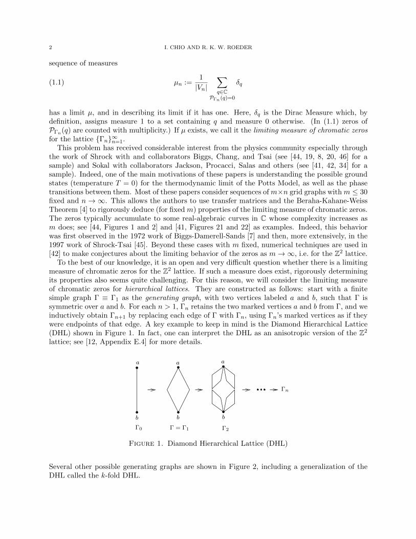
To the best of our knowledge, it is an open and very difficult question whether there is a limitingmeasure of chromatic zeros for the Z2 lattice. If such a measure does exist, rigorously determiningits properties also seems quite challenging. For this reason, we will consider the limiting measureof chromatic zeros for hierarchical lattices. They are constructed as follows: start with a finitesimple graph Γ ≡ Γ1 as the generating graph, with two vertices labeled a and b, such that Γ issymmetric over a and b. For each n > 1, Γn retains the two marked vertices a and b from Γ, and weinductively obtain Γn+1 by replacing each edge of Γ with Γn, using Γn’s marked vertices as if theywere endpoints of that edge. A key example to keep in mind is the Diamond Hierarchical Lattice(DHL) shown in Figure 1. In fact, one can interpret the DHL as an anisotropic version of the Z2

lattice; see [12, Appendix E.4] for more details.

b bb

aa a

Γn

Γ0 Γ2Γ = Γ1

Figure 1. Diamond Hierarchical Lattice (DHL)

Several other possible generating graphs are shown in Figure 2, including a generalization of theDHL called the k-fold DHL.

CHROMATIC ZEROS ON HIERARCHICAL LATTICES AND EQUIDISTRIBUTION ON PARAMETER SPACE 3

Statistical physics on hierarchical lattices dates back to the work of Berker and Ostlund [5],followed by Griffiths and Kaufman [31], Derrida, De Seze, and Itzykson [24], Bleher and Zalys[14, 16, 15], and Bleher and Lyubich [13].

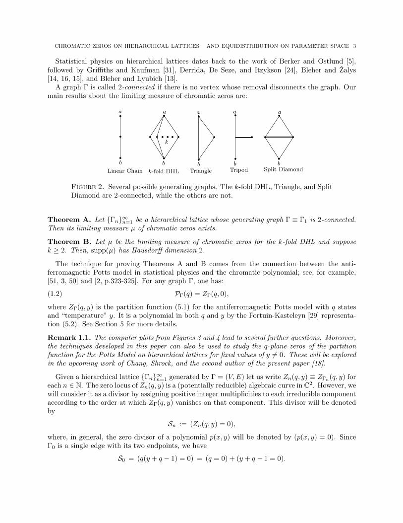
A graph Γ is called 2-connected if there is no vertex whose removal disconnects the graph. Ourmain results about the limiting measure of chromatic zeros are:

k

a

b

Linear Chain Tripod

a

bSplit Diamond

a

b

k-fold DHL Triangle

a a

b b

Figure 2. Several possible generating graphs. The k-fold DHL, Triangle, and SplitDiamond are 2-connected, while the others are not.

Theorem A. Let Γn∞n=1 be a hierarchical lattice whose generating graph Γ ≡ Γ1 is 2-connected.Then its limiting measure µ of chromatic zeros exists.

Theorem B. Let µ be the limiting measure of chromatic zeros for the k-fold DHL and supposek ≥ 2. Then, supp(µ) has Hausdorff dimension 2.

The technique for proving Theorems A and B comes from the connection between the anti-ferromagnetic Potts model in statistical physics and the chromatic polynomial; see, for example,[51, 3, 50] and [2, p.323-325]. For any graph Γ, one has:

PΓ(q) = ZΓ(q, 0),(1.2)

where ZΓ(q, y) is the partition function (5.1) for the antiferromagnetic Potts model with q statesand “temperature” y. It is a polynomial in both q and y by the Fortuin-Kasteleyn [29] representa-tion (5.2). See Section 5 for more details.

Remark 1.1. The computer plots from Figures 3 and 4 lead to several further questions. Moreover,the techniques developed in this paper can also be used to study the q-plane zeros of the partitionfunction for the Potts Model on hierarchical lattices for fixed values of y 6= 0. These will be exploredin the upcoming work of Chang, Shrock, and the second author of the present paper [18].

Given a hierarchical lattice Γn∞n=1 generated by Γ = (V,E) let us write Zn(q, y) ≡ ZΓn(q, y) foreach n ∈ N. The zero locus of Zn(q, y) is a (potentially reducible) algebraic curve in C2. However, wewill consider it as a divisor by assigning positive integer multiplicities to each irreducible componentaccording to the order at which ZΓ(q, y) vanishes on that component. This divisor will be denotedby

Sn := (Zn(q, y) = 0),

where, in general, the zero divisor of a polynomial p(x, y) will be denoted by (p(x, y) = 0). SinceΓ0 is a single edge with its two endpoints, we have

S0 = (q(y + q − 1) = 0) = (q = 0) + (y + q − 1 = 0).


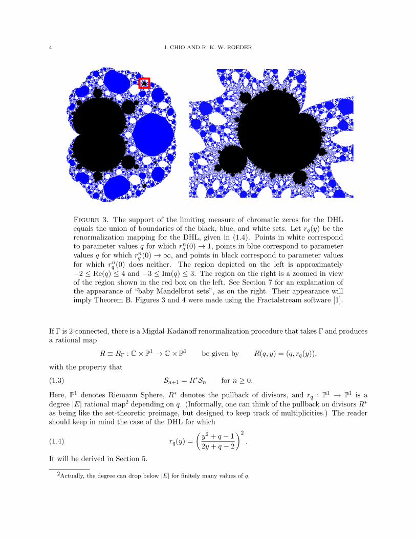
Figure 3. The support of the limiting measure of chromatic zeros for the DHLequals the union of boundaries of the black, blue, and white sets. Let rq(y) be therenormalization mapping for the DHL, given in (1.4). Points in white correspondto parameter values q for which rnq (0)→ 1, points in blue correspond to parametervalues q for which rnq (0) → ∞, and points in black correspond to parameter valuesfor which rnq (0) does neither. The region depicted on the left is approximately−2 ≤ Re(q) ≤ 4 and −3 ≤ Im(q) ≤ 3. The region on the right is a zoomed in viewof the region shown in the red box on the left. See Section 7 for an explanation ofthe appearance of “baby Mandelbrot sets”, as on the right. Their appearance willimply Theorem B. Figures 3 and 4 were made using the Fractalstream software [1].

If Γ is 2-connected, there is a Migdal-Kadanoff renormalization procedure that takes Γ and producesa rational map

R ≡ RΓ : C× P1 → C× P1 be given by R(q, y) = (q, rq(y)),

with the property that

Sn+1 = R∗Sn for n ≥ 0.(1.3)

Here, P1 denotes Riemann Sphere, R∗ denotes the pullback of divisors, and rq : P1 → P1 is adegree |E| rational map2 depending on q. (Informally, one can think of the pullback on divisors R∗

as being like the set-theoretic preimage, but designed to keep track of multiplicities.) The readershould keep in mind the case of the DHL for which

rq(y) =

(y2 + q − 1

2y + q − 2

)2

.(1.4)

It will be derived in Section 5.

2Actually, the degree can drop below |E| for finitely many values of q.


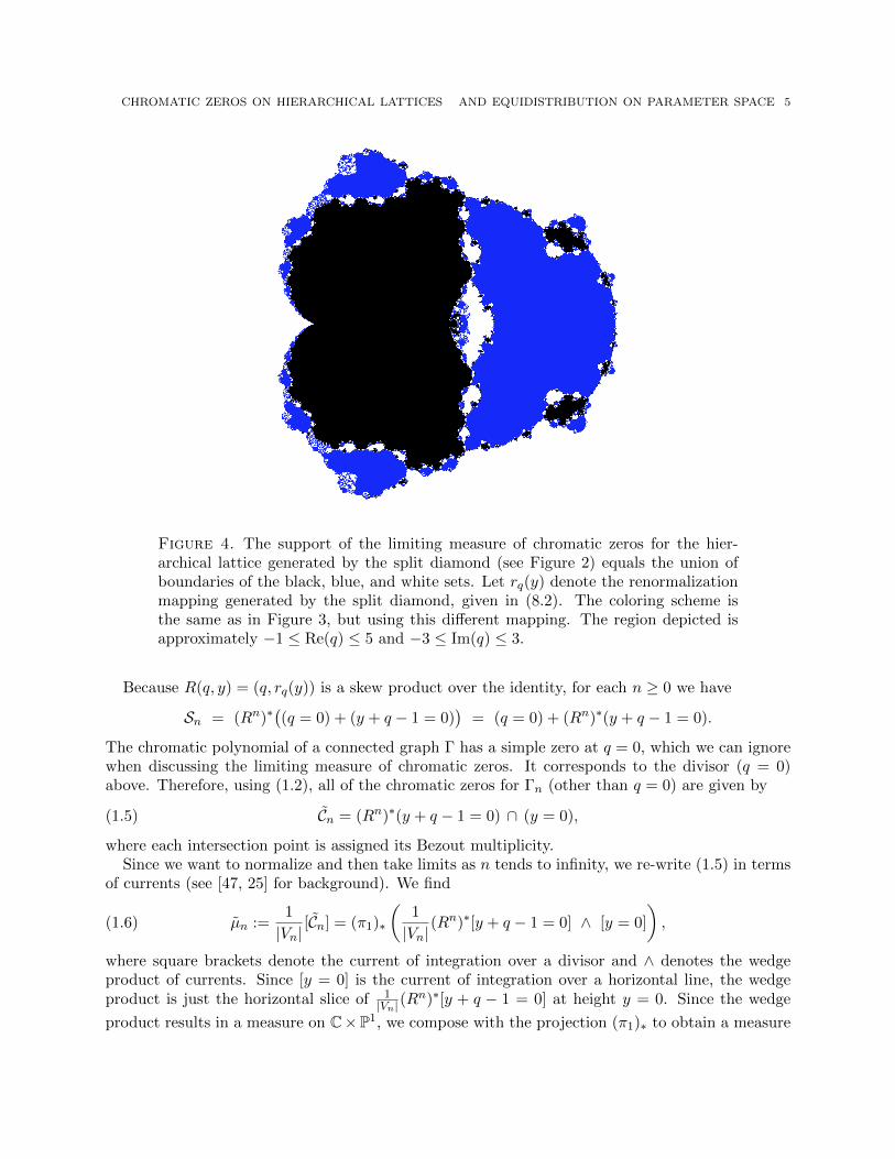
Figure 4. The support of the limiting measure of chromatic zeros for the hier-archical lattice generated by the split diamond (see Figure 2) equals the union ofboundaries of the black, blue, and white sets. Let rq(y) denote the renormalizationmapping generated by the split diamond, given in (8.2). The coloring scheme isthe same as in Figure 3, but using this different mapping. The region depicted isapproximately −1 ≤ Re(q) ≤ 5 and −3 ≤ Im(q) ≤ 3.

Because R(q, y) = (q, rq(y)) is a skew product over the identity, for each n ≥ 0 we have

Sn = (Rn)∗((q = 0) + (y + q − 1 = 0)

)= (q = 0) + (Rn)∗(y + q − 1 = 0).

The chromatic polynomial of a connected graph Γ has a simple zero at q = 0, which we can ignorewhen discussing the limiting measure of chromatic zeros. It corresponds to the divisor (q = 0)above. Therefore, using (1.2), all of the chromatic zeros for Γn (other than q = 0) are given by

Cn = (Rn)∗(y + q − 1 = 0) ∩ (y = 0),(1.5)

where each intersection point is assigned its Bezout multiplicity.Since we want to normalize and then take limits as n tends to infinity, we re-write (1.5) in terms

of currents (see [47, 25] for background). We find

µn :=1

|Vn|[Cn] = (π1)∗

(1

|Vn|(Rn)∗[y + q − 1 = 0] ∧ [y = 0]

),(1.6)

where square brackets denote the current of integration over a divisor and ∧ denotes the wedgeproduct of currents. Since [y = 0] is the current of integration over a horizontal line, the wedgeproduct is just the horizontal slice of 1

|Vn|(Rn)∗[y + q − 1 = 0] at height y = 0. Since the wedge

product results in a measure on C×P1, we compose with the projection (π1)∗ to obtain a measure


on C. (In the previous two paragraphs we have used tildes on Cn and µn to denote that we havedropped the simple zero at q = 0.)

It is relatively standard to see that

1

|En|(Rn)∗[y + q − 1 = 0]→ T,

where T is the fiber-wise Green current for the family of rational maps rq(y). In Proposition 5.4

we’ll see that α := limn→∞|En||Vn| exists so that

Tn :=1

|Vn|(Rn)∗[y + q − 1 = 0]→ αT.

However:

First Main Technical Issue: Tn → αT does not necessarily imply Tn ∧ [y = 0]→ αT ∧ [y = 0].

This issue will be handled using the notion of activity currents which were introduced by DeMarcoin [22] to study bifurcations in families of rational maps (they are sometimes called bifurcationcurrents). Since then, they have been studied by Berteloot, DeMarco, Dujardin, Favre, Gauthier,Okuyama and many others. We refer the reader to the surveys by Berteloot [6] and Dujardin [27]for further details.

We can re-write (1.6) as

µn :=1

|Vn|[(rnq a)(q) = b(q)],

where a, b : C→ P1 are the two marked points

a(q) = 0 and b(q) = 1− q.(Special care must be taken at the finitely many parameters q for which degy(rq(y)) < |E|. It isthe Second Main Technical Issue for proving Theorem A and it will be be explained in the nextsubsection.)

Meanwhile, the activity current of the marked point a is defined by

Ta := limn→∞

1

|En|(rnq a)∗ω,

where ω is the fiberwise Fubini-Study (1, 1) form on C×P1. Therefore, proving Theorem A reducesto proving the convergence

µn =1

|Vn|[(rnq a)(q) = b(q)]→ αTa.(1.7)

It will be a consequence of Theorems C and C’ that are presented in the next subsection.

1.2. Equidistribution in parameter space. Let V be a connected projective algebraic manifold.An algebraic family of rational maps of degree d is a rational mapping

f : V × P1 99K P1

such that, there exists an algebraic hypersurface Vdeg ⊂ V (possibly reducible) with the propertythat for each λ ∈ V \ Vdeg the mapping

fλ : P1 → P1 defined by fλ(z) = f(λ, z)

is a rational map of degree d. A marked point is a rational map a : V 99K P1. (We will denote theindeterminacy locus of a by I(a). It is a proper subvariety of codimension at least two.)


Our result will depend heavily on a theorem from arithmetic dynamics due to Silverman [48,Theorem E] and this will require us to assume that the manifold V , the family f , and the markedpoints a and b are defined over the algebraic numbers Q. In other words, every polynomial in thedefinitions of these objects has coefficients in Q.

Convention. Throughout the paper an algebraic family of rational maps f : V ×P1 99K P1 definedover Q will mean that both V and f are defined over Q.

Theorem C. Let f : V ×P1 99K P1 be an algebraic family of rational maps of degree d ≥ 2 definedover Q and let a, b : V 99K P1 be two marked points defined over Q. Extending Vdeg, if necessary,we can suppose I(a) ∪ I(b) ⊂ Vdeg.

Suppose that:

(i) There is no iterate n satisfying fnλ a(λ) ≡ b(λ).(ii) The marked point b(λ) is not persistently exceptional for fλ.

Then we have the following convergence of currents on V \ Vdeg

(1.8)1

dn[(fnλ a)(λ) = b(λ)]→ Ta,

where Ta is the activity current of the marked point a(λ).

The precise definition of activity current will be given in Section 2.The following version of Theorem C holds on all of V , without removing Vdeg, an essential feature

for our application to Theorem A.

Theorem C’. Let f : V ×P1 99K P1 be an algebraic family of rational maps of degree d ≥ 2 definedover Q and let a, b : V 99K P1 be two marked points defined over Q. Suppose that

(i) There is no iterate n satisfying fnλ a(λ) ≡ b(λ).(ii) The marked point b(λ) is not persistently exceptional for fλ.

Consider the rational map

F : V × P1 99K V × P1 defined by F (λ, z) = (λ, f(λ, z)).

Then the following sequence of currents on V

(1.9) (π1)∗

(1

dn(Fn)∗ [z = b(λ)] ∧ [z = a(λ)]

)converges and the limit equals Ta when restricted to V \ Vdeg. Here, π1 : V × P1 → P1 is theprojection onto the first coordinate π1(λ, z) = λ.

Remark 1.2. We have phrased Theorems C and C’ in their natural level of generality. However, inmost applications that we have in mind (in particular to the chromatic zeros), one can use V = Pmand define everything in the usual affine coordinates Cm ⊂ Pm in the following ways:

(i) f(λ, z) = P (λ,z)Q(λ,z) with P,Q ∈ Q[λ, z] and having no common factors of positive degree in

Q[λ, z], and

(ii) a(λ) = R(λ)S(λ) with R,S ∈ Q[λ] and having no common factors of positive degree in Q[λ] (and

similarly for b(λ)).

The reader can keep in mind the simple case of the renormalization mapping for the DHL (1.4) inwhich case everything is defined over Q ⊂ Q. Here V = P1,

(i) r(q, y) =(y2+q−12y+q−2

)2,


(ii) a(q) ≡ 0, and b(q) = 1− q.The degree of this family is d = 4 and Vdeg = 0,∞ because the degree of rq(y) drops when q = 0and q =∞ but at no other values of q.

The proofs of Theorem C and C’ will closely follow the strategy that Dujardin-Favre use in [28,Theorem 4.2]. However:

Second Main Technical Issue: The proof of [28, Theorem 4.2] requires a technical “Hypothe-sis (H)” that is not satisfied for the Migdal-Kadanoff renormalization mapping (1.4) for the DHL(and presumably not satisfied for many other hierarchical lattices). Indeed, q = 0 ∈ Vdeg for thismapping and there are active parameters accumulating to q = 0. One sees this in Figure 3 whereq = 0 is the “main cusp” on the left side of the black region.

Our assumption that the family and the marked points are defined over Q allows us to avoidHypothesis (H). Note that, using quite different techniques, Okuyama has proved in [38, Theorem 1]a version of [28, Theorem 4.2] without Hypothesis (H). His proof requires the marked point to becritical, but does not require working over Q.

Once Theorem C is proved, one can extend the convergence (1.8) across Vdeg by an applicationof the compactness theorem for families of plurisubharmonic functions [33, Theorem 4.1.9], thusproving Theorem C’. Note that a similar statement to Theorem C’ is found in the work of Gauthier-Vigny [30, Corollary 3.1]. The proof there also uses such compactness to extend a given convergenceacross various “bad” parameters that are analogous to our Vdeg.

1.3. Recent works on interplay between holomorphic dynamics and statistical physics.The present work lies in the context of several recent papers where holomorphic dynamics hasplayed a role in studying problems from statistical physics. We describe a sample of them here.

One can interpret a rooted Cayley Tree as a type of hierarchical lattice, and this allows one toapply a renormalization theory that is similar to the Migdal-Kadanoff version used in this paper,in order to study statistical physics on such trees. This led to holomorphic dynamics playing animportant role in proof of the Sokal Conjecture by Peters and Regts [40] and also in their work onthe location of Lee-Yang zeros for bounded degree graphs [39]. The same renormalization theorywas also recently used in combination with techniques from dynamical systems by He, Ji, and theauthors of the present paper to characterize the limiting measure of Lee-Yang zeros for the CayleyTree [21].

Meanwhile, holomorphic dynamics has been used by Bleher, Lyubich, and the second author ofthe present paper to characterize the limiting measure of Lee-Yang zeros for the DHL [12] and alsoto describe the limit behavior of the Lee-Yang-Fisher zeros for the DHL [11].

1.4. Structure of the paper. In Section 2 we present background on activity currents and de-scribe the Dujardin-Favre classification of the passive locus, that will play an important role in theproofs of Theorems C and C’. Theorems C and C’ are proved in Section 3 and Section 4.

We return to the problem of chromatic zeros in Section 5 by providing background on theirconnection with the Potts Model from statistical physics. We also set up the renormalizationmapping rq(y) associated to any hierarchical lattice having 2-connected generating graph. Weprove Theorem A in Section 6 by verifying the hypotheses of Theorem C’.

For the k-fold DHL with k ≥ 2, one can check that the critical points y = ±√

1− q satisfyrq(±

√1− q) ≡ 0 ≡ a(q). Therefore, a result of McMullen [36, Theorem 1.1] gives that supp(Ta)

has Hausdorff dimension 2. This is explained in Section 7, where we prove Theorem B.


We conclude the paper with Section 8 were we discuss the chromatic zeros associated with thehierarchical lattices generated by each of the graphs shown in Figure 2. We also provide a moredetailed explanation of Figures 3 and 4.

Acknowledgments: We are very grateful to Robert Shrock for introducing us to the problem ofunderstanding the limiting measure of chromatic zeros for a lattice and for several helpful commentsabout our paper. We are also very grateful to Laura DeMarco and Niki Myrto Mavraki who havegiven us guidance on arithmetic dynamics and also provided the details from Subsection 4.2 (Arith-metic proof of Proposition 4.2) as well as Proposition 7.2. We also thank Romain Dujardin, CharlesFavre, Thomas Gauthier, and Juan Rivera-Letelier for interesting discussions and comments. Thiswork was supported by NSF grant DMS-1348589.

2. Basics in Activity Currents

2.1. Activity Current for Holomorphic Families. Let Λ be a connected complex manifold.A holomorphic family of rational maps of degree d ≥ 2 is a holomorphic map f : Λ × P1 → P1

such thatfλ := f(λ, ·) : P1 → P1 is a rational map of degree d for every λ ∈ Λ. In this context, amarked point is just a holomorphic map a : Λ → P1. Remark that if one starts with an algebraicfamily of rational maps f : V × P1 99K P1 one can delete Vdeg to obtain a holomorphic familyf : (V \ Vdeg)× P1 → P1.

The marked point a : Λ→ P1 is called passive at λ0 ∈ Λ if the family fnλ a(λ) is normal in someneighborhood of λ0, otherwise a is said to be active at λ0. The set of active parameters is calledthe active locus. The active locus naturally supports an invariant current Ta which we will describenow. (Classically, one usually chooses a to be a marked critical point, but it is not necessary.)

Associated to a holomorphic family fλ of rational maps with degree d ≥ 2 is a skew productmapping

F : Λ× P1 → Λ× P1 given by F (λ, z) = (λ, fλ(z)).(2.1)

Let ω be the Fubini-Study (1, 1) form on P1 and let ω = π∗2ω, where π2(λ, z) = z is the projectiononto the second coordinate. The next proposition and corollary are standard results in complexdynamics, see for example [28, Proposition 3.1].

Proposition 2.1. The sequence of closed positive (1, 1) currents, d−n(Fn)∗ω, converges to a closed

positive (1, 1) current T .

Let vn, v∞ be the local potentials of d−n(fn)∗ω and T respectively. In the proof of Proposition 2.1one sees that that vn → v∞ locally uniformly, which implies the following corollary:

Corollary 2.2. For any marked point a : Λ→ P1, we have the following convergence of intersectionof currents:

(2.2)1

dn(fn)∗ω ∧ [z = a(λ)]→ T ∧ [z = a(λ)] .

Let Γ := (λ, a(λ) ⊂ Λ× P1. Since π1 : Γ→ Λ is an isomorphism, one defines the activity currentof the pair (f, a) by

(2.3) Ta := (π1)∗

(T ∧ [z = a(λ)]

).

The next result can be found in [28, Theorem 3.2], in which it was assumed that a(λ) is a markedcritical point. However, one can check that its proof does not rely on the fact that the markedpoint is critical.

Theorem 2.3. The support of the activity current Ta coincides with the active locus of a.


2.2. Activity Current for Algebraic Families. Let f : V × P1 99K P1 be an algebraic familyof rational maps of degree d. The construction from the previous subsection defines the activitycurrent Ta for the corresponding holomorphic family f : (V \ Vdeg) × P1 → P1. We will now showthat there is a natural extension of Ta through the hypersurface Vdeg.

As the construction is local, without loss of generality we can suppose V is an open subset of Cm.We can choose a lift f : V × C2 → C2 which is holomorphic and so that for each λ ∈ V ,

fλ(z, w) := f(λ, z, w) = (Pλ(z, w), Qλ(z, w)),

where Pλ, Qλ are homogeneous polynomials. Moreover, Pλ, Qλ have degree d′ ≤ d, with equalityiff λ ∈ V \ Vdeg. Similarly, the marked point a : V 99K P1 can be lifted to a holomorphic map

a : V → C2.

Let Gn : V → [−∞,∞) be the PSH function defined by

Gn(λ) :=1

dnlog ||(fnλ a)(λ)||.

Proposition 2.4. Suppose V ⊂ Cm is open. The pointwise limit

G(λ) := limn→∞

Gn(λ)

exists and is PSH in V . When restricted to V \ Vdeg, the current Ta := ddcG is identically equal tothe activity current Ta.

Remark 2.5. On V \ Vdeg the functions Gn(λ) correspond to local potentials for the currents onthe left side of (2.2) from Corollary 2.2 and the limiting function G(λ) corresponds to the localpotential for the current on the right side of (2.2). In particular, on V \ Vdeg the continuousfunctions Gn(λ) converge locally uniformly to the continuous function G(λ) and the latter is notequal to −∞ anywhere. See the proof of [28, Proposition 3.1] for details.

Proof. Fix a parameter λ ∈ V so that fλ : P1 → P1 is a rational map with degree d′ ≤ d. Since itslift fλ is defined up to a multiplicative constant, we may assume that in the unit sphere S ⊂ C2

we have supS |fλ| = 1. By the homogeneity of fλ,

||fλ(z, w)|| ≤ ||(z, w)||d′ , which implies ||fn+1λ (z, w)|| ≤ ||fnλ (z, w)||d′ ,

so the maps Gn satisfy

Gn+1(λ) =1

dn+1log ||(fn+1

λ a)(λ)|| ≤ 1

dn+1log ||(fnλ a)(λ)||d′ ≤ 1

dnlog ||(fnλ a)(λ)|| = Gn(λ),

which implies that Gn∞n=1 is a decreasing sequence of PSH functions, so it either converges to aPSH limit function G or to −∞ identically. The latter is impossible, by Remark 2.5.

Proposition 2.6. Suppose V ⊂ Cm is open. The sequence of PSH functions Gn converges to Gin L1

loc(V ). Equivalently, the sequence of currents ddcGn converges to Ta = ddcG.

Proof. Assume on the contrary that Gn 6→ G in L1loc(V ). Then the compactness theorem for PSH

functions [33, Theorem 4.1.9] implies that there is a subsequence Gnk and some PSH functionG′ 6= G in L1

loc(V ) such that Gnk → G′ in L1loc(V ). Then there is a set Ω ⊂ V of positive measure

in which G′(λ) 6= G(λ) for all λ. In particular, since Vdeg is a hypersurface and hence has zeromeasure, we can find a compact set K ⊂ Ω \ Vdeg in which Gnk → G′. However, by Corollary 2.2,Gn → G uniformly in K, which is a contradiction.


2.3. Classification of the Passivity Locus.

Dujardin-Favre Classification of Passivity Locus [28, Theorem 4]. Let f : Λ× P1 → P1 bea holomorphic family and let a(λ) be a marked point. Assume U ⊂ Λ is a connected open subsetwhere a(λ) is passive. Then exactly one of the following cases holds:

(i) a(λ) is never preperiodic in U . In this case the closure of the orbit of a(λ) can be followedby a holomorphic motion.

(ii) a(λ) is persistently preperiodic in U .(iii) There exists a persistently attracting (possibly superattracting) cycle attracting a(λ) through-

out U and there is a closed subvariety U ′ ( U such that the set of parameters λ ∈ U \ U ′for which a(λ) is preperiodic is a proper closed subvariety in U \ U ′.

(iv) There exists a persistently irrationally neutral periodic point such that a(λ) lies in the in-terior of its linearization domain throughout U and the set of parameters λ ∈ U for whicha(λ) is preperiodic is a proper closed subvariety in U .

This classification is stated in [28] with the marked point being critical. However, the heart ofthe proof is a separate theorem (Theorem 1.1 in [28]) whose statement does not require the markedpoint to be critical. Meanwhile, the remainder of the proof is short and it is easy to check that themarked point need not be critical.

However, one should note that the statement in [28] claims that in Case (iii) the set λ suchthat a(λ) is preperiodic is a closed subvariety of U itself, without first removing a proper closedsubvariety U ′. Unfortunately, that is not true, but fortunately that particular claim is not usedanywhere later in their paper.

Consider the following holomorphic family of polynomial mappings

fλ(z) = z(z − λ)(z − 1/2)

where λ ∈ C. The critical points of fλ are

c±(λ) =(1 + 2λ)±

√4λ2 − 2λ+ 1

6,

which vary holomorphically in a neighborhood Dr(0) of λ = 0, for some r > 0. Notice that c−(0) = 0and c+(0) = 1

3 . Consider the marked critical point c(λ) := c+(λ). One can check that

(1) There exists 0 < ε < r such that λ ∈ Dε(0) implies that fnλ (c(λ))→ 0 with |fnλ (c(λ))| < 1/2for all n ≥ 0, and

(2) There exists an infinite sequence λk∞k=1 in Dε(0) \ 0 with λk → 0 such that for each kthere is an iterate nk with fnkλk (c(λk)) = 0.

Therefore, the set of preperiodic parameters λ ∈ Dε(0) is not a closed subvariety, but they are inDε(0) \ 0.

Proof of the claim about preperiodic parameters in Case (iii): By taking a suitable iterate, let ussuppose that a(λ) is attracted to an attracting fixed point p(λ). For each λ ∈ U let m(λ) denotethe local multiplicity of p(λ) for fλ. Let m0 := minm(λ) : λ ∈ U and let

U ′ := λ ∈ U : m(λ) > m0.

Suppose λ0 ∈ U \ U ′ and choose a neighborhood W of λ0 such that W b U \ U ′. Then, thereexists ε > 0 such that:

(i) fλ(Dε(p(λ)) b Dε(p(λ)), and(ii) for each λ ∈W and each z ∈ Dε(p(λ)) \ p(λ) we have that fλ(z) 6= p(λ),

i.e. p(λ) is the only preimage of p(λ) under fλ within Dε(p(λ)).


Since W is compact and fnλ (a(λ)) → p(λ) for all λ ∈ W there exists k > 0 such that for all

λ ∈W we have that fkλ (a(λ)) ⊂ Dε(p(λ)). Then, using (ii) above, the set of preperiodic parametersin W is

λ ∈W : fnλ (a(λ)) = p(λ) for some 0 ≤ n ≤ k,which is a closed subvariety of W .

3. Proof of Theorem C

Our proof of Theorem C will closely follow the strategy that Dujardin-Favre use to prove Theo-rem 4.2 in [28] and we will assume some of the basic results from their proof.

Let f : V × P1 99K P1 be an algebraic family of rational maps of degree d defined over Q. Leta, b : V 99K P1 be marked points and assume, without loss of generality, that the indeterminacyI(a) ∪ I(b) ⊂ Vdeg. Let Ta be the activity current of a(λ) and suppose that all hypotheses ofTheorem C are satisfied.

Proposition 3.1. The following convergence of currents

(3.1)1

dn[(fnλ a)(λ) = b(λ)]→ Ta

holds in V \ Vdeg if and only if there is a dense set of parameters λ ∈ Vgood ⊂ V \ Vdeg such that

hn(λ) :=1

dnlog distP1 (fnλ a(λ), b(λ))→ 0,(3.2)

where distP1 denotes the chordal distance on P1.

Proof. A direct adaptation of the first four paragraphs of the proof of Theorem 4.2 in [28] showsthat (3.1) holds if and only if hn → 0 in L1

loc(V \ Vdeg). If hn 6→ 0 in L1loc(V \ Vdeg), then, as in

paragraph seven of the same proof, one uses Hartogs’ Lemma [33, Theorem 4.1.9(b)] to find anopen set U ⊂ V \ Vdeg and a subsequence nk such that hnk(λ)→ h(λ) < 0 for all λ ∈ U .

The proof of Theorem C will then follow immediately from the following:

Proposition 3.2. There is a dense set of parameters λ ∈ Vgood ⊂ V \ Vdeg such that (3.2) holds.

This is almost an immediate consequence of the following beautiful theorem:

Silverman’s Theorem E [48]. Let φ : P1 → P1 be a rational map of degree d ≥ 2 defined over anumber field K. Let A,B ∈ P1(K) and assume that B is not exceptional for φ and that A is notpreperiodic for φ. Then

limn→∞

δ(φnA,B)

dn= 0,(3.3)

where δ(P,Q) = 2− log distP1(P,Q) is the logarithmic distance function3.

Remark that (3.3) holds if and only if limn→∞1dn log distP1(φnA,B) = 0.

If we want to use Silverman’s Theorem E directly, we need that there is a dense set of parametersV∞ ⊂ V \ Vdeg such that the marked point a(λ) has infinite orbit under fλ for all λ ∈ V∞. We donot know if this true at this level of generality, even if the active locus is non-empty.

3In [48, Theorem E] a different logarithmic distance function was used. However, as mentioned in Section 3 of thereferenced paper, the result still holds if we use 2− distP1(·, ·) instead.


3.1. Proof of Proposition 3.2. We will need the following result:

Algebraic Points Are Dense. Let V ⊂ Pn be a projective algebraic manifold that is definedover Q. Then, the set of points a ∈ V that can be represented by homogeneous coordinates in Qform a dense subset of V (in the complex topology). I.e. V (Q) is dense in V .

We could not find this statement in the literature, but it can be proved by induction on dim(V ).The base of the induction, when dim(V ) = 0, plays an important role in the theory of KleinianGroups, see for example [35, Lemma 3.1.5].

Proof of Proposition 3.2. We will consider the active and passive loci separately. Let λ0 be anactive parameter, and W ⊂ V be any open neighborhood containing λ0. We will find a parameterλ1 ∈ W at which (3.2) holds. We will do this by showing that there exists a parameter λ1 ∈ Wsuch that iterates of a(λ1) under fλ1 will eventually land on a repelling cycle disjoint from b(λ1).This will immediately imply (3.2) at λ1.

Pick three distinct points in a repelling cycle of fλ0 which is disjoint from b(λ0). By reducingW to a smaller neighborhood of λ0 if necessary, we can ensure that the repelling cycle movesholomorphically as λ varies over W , and that b(λ) is disjoint from the cycle for every λ ∈W . Sincethe family fnλ a(λ)∞n=1 is not normal in W , it cannot avoid all three points.

We now suppose λ0 is in the passive locus for a and let U be the connected component of thepassive locus containing λ0. Then, the Dujardin-Favre classification gives four possible behaviorsfor fnλ (a(λ)) in U .

In Cases (i),(iii), and (iv) the classification gives a (possibly empty) closed subvariety U ′ ( U suchthat the set of parameters for which a(λ) is preperiodic is contained in a proper closed subvarietyU1 ⊂ (U \ U ′). Moreover, the hypothesis that marked point b(λ) is not persistently exceptionalgives that there is another proper closed subvariety U2 ⊂ U such that b(λ) is not exceptional forλ ∈ U \ U2. Then, U \ (U ′ ∪ U1 ∪ U2) is an open dense subset of U . Since V (Q) is dense in V ,see the beginning of this subsection, arbitrarily close to λ0 is a point λ1 ∈ U \ (U ′ ∪ U1 ∪ U2) withcoordinates in Q. Since there are only finitely many coefficients to consider, we can find a numberfield K so that fλ1 ∈ K(z) and the points a(λ1), b(λ1) ∈ P1(K). Since λ1 ∈ U \ (U ′ ∪ U1 ∪ U2),the point a(λ1) has infinite orbit under fλ1 , and the point b(λ1) is not exceptional for fλ1 . HenceSilverman’s Theorem E implies that (3.2) holds for the parameter λ1.

Finally suppose we are in Case (ii), so that the marked point a(λ) is persistently preperiodic.By assumption there is no iterate n with fnλ (a(λ)) ≡ b(λ), so there is a proper closed subvarietyU1 ⊂ U such that for all λ ∈ U \ U1 and all n ≥ 0, we have fnλ (a(λ)) 6= b(λ). It follows thatfor each λ ∈ U \ U1, the quantities distP1(fnλ (a(λ)), b(λ)) are uniformly bounded in n ≥ 0, whichimplies (3.2) for all λ ∈ U \ U1.

3.2. Arithmetic proof of Proposition 3.2 under additional hypotheses. The additionalhypotheses are:

(iii) The parameter space is P1.(iv) The marked point a is not passive on all of P1 \ Vdeg.

For applications in chromatic zeros our parameter space is P1 so that Hypothesis (iii) will auto-matically hold (in fact, we typically think of it as C ⊂ P1). Meanwhile, for the renormalizationmappings associated with many hierarchical lattices one can check Hypothesis (iv) directly, but itdoes not hold for all such mappings (e.g. when the generating graph is a triangle, as discussed inSection 8.3).

The proof will not depend on the Dujardin-Favre classification of the passive locus but insteadrequires technical results from arithmetic dynamics. Proposition 3.2 will follow from Silverman’s


Theorem E and the next statement (choosing K to be dense in C), which is due to Laura DeMarcoand Niki Myrto Mavraki.

Proposition 3.3. (DeMarco-Mavraki) Suppose the hypotheses in Theorem C and additionallyhypotheses (iii) and (iv) above. Then, for any number field K there are at most finitely manyparameters λ ∈ P1(K) \ Vdeg such that the marked point a(λ) is preperiodic under fλ.

We will need the following two results, which depend on having a one-dimensional parameterspace. Denote the logarithmic absolute Weil height on Q by h : Q → R. For a rational mapφ : P1 → P1 defined over K and a point P ∈ P1(K), we denote the canonical height function

associated to φ by hφ(P ). For more background on these definitions, see [49].

Call-Silverman Specialization [17, Theorem 4.1]. Let (f, a) be a one-dimensional algebraicfamily of rational maps of degree d ≥ 2 with a marked point a, both defined over a number field K.Then, for any sequence of parameters λn∞n=1 ⊂ P1(K) \ Vdeg such that h(λn)→∞, we have

limn→∞

hfλn (a(λn))

h(λn)= hf (a),

where hf (a) is the canonical height associated to the pair (f, a).

The canonical height of the pair hf (a) was introduced in [17].The pair (f, a) is called isotrivial if there exists a branched covering W → P1 \Vdeg and a family

of holomorphically varying Mobius transformations Mλ such that Mλ fλ M−1λ is independent of

λ ∈W and also Mλ a is a constant function of λ ∈W .

Theorem 3.4. (DeMarco [23, Theorem 1.4]) Suppose f : P1 × P1 99K P1 is a non-isotrivial

one-dimensional algebraic family of rational maps. Let hf : P1(k)→ R be a canonical height of f ,defined over the function field k = C(P1). For each a ∈ P1(k), the following are equivalent:

(1) The marked point a is passive in all of P1 \ Vdeg;

(2) hf (a) = 0;(3) (f, a) is preperiodic.

Moreover, the set

a ∈ P1(k) : a is passive in all of P1 \ Vdegis finite.

Proof of Proposition 3.3. Assume on the contrary that there is a sequence of distinct parametersλn∞n=1 ⊂ P1(K) \ Vdeg such that a(λn) is preperiodic for fλn . It follows from Northcott property[49, Theorem 3.7] that the parameters λn satisfies h(λn)→∞. Meanwhile, since a(λn) is preperi-

odic for fλn , we have hfλn (a(λn)) = 0. Then Call-Silverman Specialization implies hf (a) = 0, so by

Theorem 3.4 the marked point a must be passive in all of P1\Vdeg, which contradicts hypothesis (iv).

4. Proof of Theorem C’

The following statement about convergence of sequences of PSH functions is probably standard,but we will include a proof because we cannot find an appropriate reference.

Proposition 4.1. Let φn∞n=1 be a sequence of PSH functions in an open connected set U ⊆ Cmwhich is uniformly bounded above in compact sets. Suppose there is a PSH function φ in U suchthat φn → φ in L1

loc(U \X), where X ⊂ U is an analytic hypersurface. Then φn → φ in L1loc(U).


Proof. Assume by contradiction that φn 6→ φ in L1loc(U). Then there is an ε > 0, a compact set K

with positive Lebesgue measure, and a subsequence φnk such that

||φnk − φ||L1(K) > ε for all k.

Note that since φn → φ in L1loc(U \X), the compact set K must intersect X. By the hypotheses, the

sequence φnk satisfies the conditions for the compactness theorem for PSH functions [33, Theorem

4.1.9], so we can find a further subsequence (which we still denote by φnk), and a PSH function φin U such that

φnk → φ in L1loc(U).

In particular φnk → φ in L1(K), which implies φ 6= φ in L1(K), so there exist δ > 0 and a

compact subset K ′ ⊂ K with positive Lebesgue measure such that |φ(z)−φ(z)| > δ for all z ∈ K ′.Let Xε be the ε-neighborhood of X in U , and let X ′ε := Xε ∩ K ′. Choose ε > 0 which satisfiesLeb(K ′) = 2Leb(X ′ε). It follows that∫

K′\X′ε

|φ− φ| dLeb > δ · Leb(K ′ \X ′ε) =δ

2Leb(K ′) > 0.(4.1)

Meanwhile, since K ′ \ X ′ε is a compact subset of U disjoint from X, we must have φ = φ inL1(K ′ \X ′ε), which contradicts (4.1).

Proof of Theorem C’. This is a local statement, so we can suppose without loss of generality that Vis an open subset of Cm. Choose a lift f : V ×C2 → C2 and denote the iterates of each fλ : C2 → C2

by

fnλ (z, w) =(P

(n)λ (z, w), Q

(n)λ (z, w)

).

Choose lifts a, b : V → C2 and denote their coordinates by a(λ) = (a1(λ), a2(λ)) and b(λ) =(b1(λ), b2(λ)).

Recall from Section 3 that

hn(λ) :=1

dnlog distP1 (fnλ a(λ), b(λ)) .(4.2)

Although (4.2) is only defined on V \ Vdeg, interpreting hn in terms of the lifts allows its extensionto all of V :

hn(λ) :=1

dnlog |P (n)

λ (a(λ))b2(λ)−Q(n)λ (a(λ))b1(λ)|2 − 1

dnlog ||(fnλ a)(λ)||2 − 1

dnlog ||b(λ)||2.

Note that the last term satisfies

1

dnlog ||b(λ)||2 → 0 in L1

loc(V ) as n→∞,

and by Proposition 2.6,

1

dnlog ||(fnλ a)(λ)||2 → 2G in L1

loc(V ) as n→∞,

where G is the local potential for Ta. Moreover, by Proposition 3.1, hn → 0 in L1loc(V \ Vdeg).

Therefore we can conclude that

1

dnlog |P (n)

λ (a(λ))b2(λ)−Q(n)λ (a(λ))b1(λ)|2 −→ 2G in L1

loc(V \ Vdeg).


Since G and the sequence 1dn log |P (n)

λ (a(λ))b2(λ) − Q(n)λ (a(λ))b1(λ)| are PSH functions in V , it

follows from Proposition 4.1 that

1

dnlog |P (n)

λ (a(λ))b2(λ)−Q(n)λ (a(λ))b1(λ)| −→ G in L1

loc(V ),

The PSH functions on the left hand side are local potentials for the currents expressed in (1.9) andG is a local potential for Ta on V \ Vdeg.

5. The Potts Model, Chromatic Zeros, and Migdal-Kadanoff Renormalization

We first give a brief account of the antiferromagnetic Potts model on a graph Γ and its connectionwith the chromatic zeros of PΓ. Suitable references include [51, 3, 50], [2, p.323-325], and referencestherein. We then describe the Migdal-Kadanoff Renormalization procedure that produces a rationalfunction rq(y) relating the zeros for the Potts Model on one level of a hierarchical lattice to thezeros for the next level. The remainder of the section is devoted to proving properties of therenormalization mappings rq(y).

5.1. Basic Setup. Fix a graph Γ = (V,E) and fix an integer q ≥ 2. A spin configuration of thegraph Γ is a map

σ : V → 1, 2, ..., q.Fix the coupling constant J < 0. The energy HΓ(σ) associated with a configuration σ on Γ isdefined as

HΓ(σ) = −J∑

vi,vj∈E

δ(σ(vi), σ(vj)) = −JE(σ),

where δ(a, b) = 1 if a = b and 0 otherwise, and E(σ) is the number of edges whose endpointsare assigned the same spin under σ. Remark that since J < 0 it is energetically favorable tohave different spins at the endpoints of each edge, if possible. This means that we are in theantiferromagnetic regime.

The Boltzmann distribution assigns a configuration σ on Γ probability proportional to the weight

WΓ(σ) = exp

(−HΓ(σ)

T

)= exp

(JE(σ)

T

),

where T > 0 is the temperature of the system 4. The probability Pr(σ) of σ occurring is therefore

(5.1) Pr(σ) = WΓ(σ)/ZΓ where ZΓ :=∑σ

WΓ(σ),

and the sum is over all possible spin configurations. Some intuition for this distribution can begained by considering the following two extreme cases: when T is near zero, configurations withminimum energy are strongly favored. Meanwhile for high temperature, all configurations occurwith nearly equal probability.

Let us introduce the temperature-like variable y := eJ/T, so that WΓ(σ) = yE(σ). All the quan-tities above implicitly depend on q, y, and the graph Γ. The normalizing factor ZΓ(q, y) is calledthe partition function and given by

ZΓ(q, y) :=∑σ

yE(σ).

4We set the Boltzmann constant kB = 1.


It turns out that ZΓ(q, y) is actually a polynomial in both q and y. To see this it will be helpful toexpress the partition function in terms of (q, v) where v = y − 1. For any subset of the edge setA ⊆ E is a subgraph (V,A). We have

(5.2) ZΓ(q, v) =∑σ

∏(i,j)∈E

[1 + vδ(σi, σj)] =∑A⊆E

qk(A)v|A|.

where k(A) is the number of connected components of (V,A), including isolated vertices. This iscalled the Fortuin-Kasteleyn [29] representation of ZΓ(q, v); see, for example, [50, Section 2.2]. (Wewill only express ZΓ in terms of v instead of y in this paragraph and in Subsection 5.2.)

As discussed in the introduction, we will describe the zeros of ZΓ(q, y) as a divisor denoted

S := (ZΓ(q, y) = 0).

Remark that in the next subsection we will see that if Γ is 2-connected, then ZΓ(q, y) = qZΓ(q, y)

with ZΓ(q, y) irreducible, implying S is a reduced divisor, i.e. all multiplicities are one. Therefore,if Γ is 2-connected there is no harm in thinking of S as a (reducible) algebraic curve.

To establish the connection between the chromatic polynomial PΓ(q) and the partition functionZΓ(q, y) of the Potts model note that

PΓ(q) =∑

σ such thatE(σ)=0

1 = ZΓ(q, 0).

Therefore, the chromatic zeros are given by the intersection:

C := S ∩ (y = 0),

where Bezout intersection multiplicities and multiplicities of the divisor S are taken into account.

5.2. Irreducibility of ZΓ(q, y) for 2-connected Γ. It follows from (5.2) that we can always factor

ZΓ(q, v) = qZΓ(q, v) in the polynomial ring C[q, v]. The goal of this subsection is to prove:

Proposition 5.1. If Γ is 2-connected, then ZΓ(q, v) is irreducible in C[q, v]. (The same holds inthe (q, y) variables.)

We will prove this proposition using the well-known relationship between ZΓ(q, y) and the TuttePolynomial of Γ. It is defined as

(5.3) TΓ(x, y) =∑A⊂E

(x− 1)k(A)−1(y − 1)|A|+k(A)−|V |,

where k(A) has the same interpretation as in (5.2). The variables (x, y) in the Tutte Polynomialare related5 to the variables (q, v) in the Partition Function (5.2) by:

x = 1 + (q/v) and y = v + 1.

Comparing (5.3) with (5.2) we see the following relationship [50, Section 2.5] between T (x, y) andZΓ(q, v):

(5.4) TΓ(x, y) = (x− 1)−1(y − 1)−|V |ZΓ((x− 1)(y − 1), y − 1).

Proposition 5.1 will be a corollary to the following nice result by de Mier, Merino, and Noyi [37].

Irreducibility Of Tutte Polynomials. If Γ is a connected matroid, in particular a 2-connectedgraph, then TΓ(x, y) is irreducible in C[x, y].

5Although the variable y appears in Equation (5.1) for the partition function and also in Equation (5.3) for theTutte Polynomial, there is no conflict of notation because both satisfy y = v + 1.


Lemma 5.2. ZΓ(q, v) vanishes to order exactly |V | at the origin.

Proof. For any subgraph (V,A), it follows from a counting argument that k(A) + |A| ≥ |V |. More-over, for the subgraph (V,A0) without any edges, the sum k(A0) + |A0| is exactly |V |. Thereforethe order of vanishing is exactly |V | at the origin.

Proof of Proposition 5.1. By the Irreducibility of the Tutte Polynomial, it suffices to prove that if

ZΓ is reducible then so is TΓ. Suppose ZΓ is reducible:

ZΓ = A1 ·A2 ·B,where A1, A2 are non-constant irreducible factors, and B can potentially be a unit. Denote by Cithe zero set of Ai.

Let H : C2 → C2 be the birational map (x, y) 7→ ((x− 1)(y− 1), y− 1), so that by (5.4) we have

TΓ(x, y) = (y − 1)−|V |+1(ZΓ H).

Therefore, in order to prove that TΓ is reducible it suffices to find at least two irreducible factorsof ZΓ H each of which is not equal to y − 1.

For i = 1 and 2, although H−1(Ci) can possibly contain the line E := (x, y) ∈ C2 : y = 1, itcannot be the only irreducible component of H−1(Ci) because H(E) is a single point (0, 0). Fromthis observation we now have to consider two separate cases.

(i) If A1 6≡ A2, then the zero set of TΓ contains at least two distinct irreducible components,neither of which is the line E.

(ii) If A1 ≡ A2, then the zero set of TΓ contains an irreducible component of multiplicity atleast two, which is not the line E.

In either case, we conclude that TΓ is reducible.

5.3. Combinatorics of Hierarchical Lattices.

Proposition 5.3. Suppose Γn∞n=1 is a hierarchical lattice that is generated by a 2-connectedgenerated graph Γ = (V,E). Then, Γn is 2-connected for each n ≥ 0.

Proof. The proof is by induction on n. Since Γ0 is a single edge with two vertices at its endpointsit is 2-connected. Suppose now that Γn is 2-connected for some n ≥ 0 to show that Γn+1 is 2-connected. Recall that Γn+1 is built by replacing each edge of the generating graph Γ with a copyof Γn using the marked vertices a and b as endpoints. The vertices of Γn+1 fall into two classes:

(1) The |V | vertices of Γn+1 that come from the vertices of Γ. Each of them is a marked vertexa or b from some copy of Γn, and

(2) The remaining vertices.

If the removal of a vertex of Type (1) disconnects Γn+1 then, since each Γn is 2-connected, thiswould imply that removal of the corresponding vertex of Γ disconnects Γ. This is impossible becauseΓ is 2-connected. Meanwhile, if removal of a vertex of Type (2) disconnects Γn+1 then its removalwill also disconnect the unique copy of Γn that the vertex is contained in. This contradicts theinduction hypothesis.

Proposition 5.4. Let Γn = (Vn, En) be a hierarchical lattice generated by generating graph Γ = (V,E).Then |Vn| and |En| grow at the same exponential rate as n→∞.

Proof. Observe that for any n ≥ 1,

|Vn+1| = |Vn|+ |En| · (|V | − 2) = |Vn|+ |E|n · (|V | − 2) .


It follows from induction that

|Vn| = |V |+ (|V | − 2) ·n−1∑i=1

|E|i = |V |+ (|V | − 2) · |E| |E|n−1 − 1

|E| − 1,

which proves the assertion.

5.4. Migdal-Kadanoff Renormalization for the DHL. Let Γn = (Vn, En)∞n=0 be the Dia-mond Hierarchical Lattice (DHL). For each n ≥ 0 the partition function Zn(q, y) ≡ ZΓn(q, y) haszero divisor

Sn := (Zn(q, y) = 0).

Remark that Γ0 is always a single edge with two vertices at its endpoints, so a simple calculationyields ZΓn(q, y) = q(y + q − 1) so that

S0 := (q(y + q − 1) = 0).

Associated to the hierarchical lattice Γn∞n=0 is a Migdal-Kadanoff renormalization mapping thatrelates the zero divisor Sn+1 to the zero divisor Sn.

Proposition 5.5. For the DHL we have that for each n ≥ 0

Sn = (Rn)∗(S0)

where R : C× P1 → C× P1 is given by

(5.5) R(q, y) = (q, rq(y)) , where rq(y) =

(y2 + q − 1

2y + q − 2

)2

.

As usual, the superscript ∗ denotes pullback of a divisor and we will denote points y ∈ P1 using thestandard chart C ⊂ P1.

The proof will be very similar to the derivation of the Migdal-Kadanoff renormalization trans-formation for the Ising Model on the DHL [12, Section 2.5] and it relies on the multiplicativity ofthe conditional partition functions which is proved in [12, Lemma 2.1], in the context of the IsingModel.

Proof. For each n ≥ 0 consider the following conditional partition functions:

Un ≡ Un(q, y) :=∑

σ such thatσ(a)=σ(b)=1

W (σ) and Vn ≡ Vn(q, y) :=∑

σ such thatσ(a)=1, σ(b)=2

W (σ).

We claim for each n ≥ 0 that

(5.6) Un+1 =(U2n + (q − 1)V2

n

)2and Vn+1 =

(2UnVn + (q − 2)V2

n

)2.

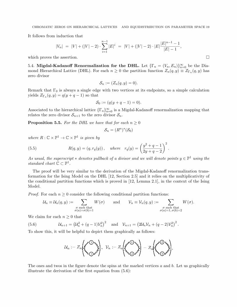
To show this, it will be helpful to depict them graphically as follows:

The ones and twos in the figure denote the spins at the marked vertices a and b. Let us graphicallyillustrate the derivation of the first equation from (5.6):


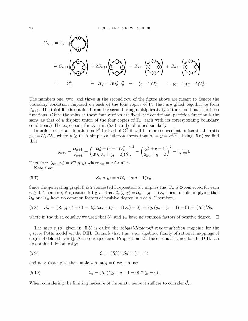
The numbers one, two, and three in the second row of the figure above are meant to denote theboundary conditions imposed on each of the four copies of Γn that are glued together to formΓn+1. The third line is obtained from the second using multiplicativity of the conditional partitionfunctions. (Once the spins at those four vertices are fixed, the conditional partition function is thesame as that of a disjoint union of the four copies of Γn, each with its corresponding boundaryconditions.) The expression for Vn+1 in (5.6) can be obtained similarly.

In order to use an iteration on P1 instead of C2 it will be more convenient to iterate the ratioyn := Un/Vn, where n ≥ 0. A simple calculation shows that y0 = y = eJ/T . Using (5.6) we findthat

yn+1 =Un+1

Vn+1=

(U2n + (q − 1)V2

n

2UnVn + (q − 2)V2n

)2

=

(y2n + q − 1

2yn + q − 2

)2

= rq(yn).

Therefore, (qn, yn) = Rn(q, y) where qn = q for all n.Note that

(5.7) Zn(q, y) = q Un + q(q − 1)Vn.

Since the generating graph Γ is 2 connected Proposition 5.3 implies that Γn is 2-connected for eachn ≥ 0. Therefore, Proposition 5.1 gives that Zn(q, y) = Un + (q− 1)Vn is irreducible, implying thatUn and Vn have no common factors of positive degree in q or y. Therefore,

Sn = (Zn(q, y) = 0) = (qn(Un + (qn − 1)Vn) = 0) = (qn(yn + qn − 1) = 0) = (Rn)∗S0,(5.8)

where in the third equality we used that Un and Vn have no common factors of positive degree.

The map rq(y) given in (5.5) is called the Migdal-Kadanoff renormalization mapping for theq-state Potts model on the DHL. Remark that this is an algebraic family of rational mappings ofdegree 4 defined over Q. As a consequence of Proposition 5.5, the chromatic zeros for the DHL canbe obtained dynamically:

Cn = (Rn)∗(S0) ∩ (y = 0)(5.9)

and note that up to the simple zero at q = 0 we can use

Cn = (Rn)∗(y + q − 1 = 0) ∩ (y = 0).(5.10)

When considering the limiting measure of chromatic zeros it suffices to consider Cn.


5.5. Migdal-Kadanoff Renormalization for arbitrary hierarchical lattices. Now supposeΓn = (Vn, En) is the hierarchical lattice generated by an arbitrary generating graph Γ = (V,E). Itis clear that we can repeat the procedure in Proposition 5.5 to produce a renormalization mappingrq(y) associated to the generating graph Γ, which is a rational map in y on the Riemann sphere ofdegree at most |E|, parameterized by polynomials in q with integer coefficients.

However, it is possible that the generic degree of rq(y) is strictly smaller than |E|. One suchexample is the Tripod shown in Figure 2 for which we have

Un+1 = (Un + (q − 1)Vn)(U2n + (q − 1)V2

n

)and Vn+1 = (Un + (q − 1)Vn)

(2UnVn + (q − 2)V2

n

).

The common factor of positive degree (Un + (q − 1)Vn) is a consequence of the “horizontal” edgethat is connected to the remainder of the generating graph Γ at a single vertex. When taking theratios yn = Un/Vn we lose track of these common factors resulting in the drop of generic degree:

R(q, y) = (q, rq(y)) where rq(y) =y2 + q − 1

2y + q − 2,

which has degree two even though Γ has three edges. This drop in generic degree results in(Rn)∗S0 < (Zn(q, y)) for the hierarchical lattice generated by the Tripod.

This phenomenon can be avoided if the generating graph is 2-connected and the proof is exactlythe same as for the DHL. We summarize:

Proposition 5.6. Let Γn∞n=0 be the hierarchical lattice generated by Γ = (V,E). If Γ is 2-connected, then the associated renormalization mapping R(q, y) = (q, rq(y)) has generic degree |E|and satisfies

Sn = (Rn)∗(S0),

where Sn = (Zn(q, y)) and S0 = (q(y + q − 1)). Moreover, rq is defined over Q.

Several concrete examples are presented in Section 8. In the proof of Theorem A we will also needthe following:

6. Proof of Theorem A

Let Γn∞n=1 be a hierarchical lattice whose generating graph Γ = (V,E) is 2-connected. De-note its Migdal-Kadanoff renormalization mapping by R(q, y) = (q, rq(y)). Since Γ is 2-conneced,Proposition 5.6 implies that the chromatic zeros for Γn (omitting the simple zero at q = 0) are

given by Cn = (Rn)∗(y + q − 1 = 0) ∩ (y = 0). Therefore, in the language of currents,

µn :=1

|Vn|∑

q∈C\0PΓn (q)=0

δq = (π1)∗

(1

|Vn|(Rn)∗[y + q − 1 = 0] ∧ [y = 0]

),

where the zeros of PΓn(q) are counted with multiplicities, as always. Since µn and µn (see (1.1))differ by 1/|Vn| times a Dirac measure at q = 0, it suffices to prove that the sequence µn converges.Moreover, Proposition 5.4 allows us to replace the normalizing factor of |Vn| with |En|. Therefore,it suffices to verify that R = (q, rq(y)) and the marked points a(q) = 0 and b(q) = 1− q satisfy thehypotheses of Theorem C’.

By Proposition 5.6, the algebraic family rq is defined over Q. Hypotheses (i) and (ii) on themarked points will be verified in Propositions 6.1 and 6.2 below.

Proposition 6.1. There are no iterates n ≥ 0 satisfying rnq (0) ≡ 1− q.


Proof. Away from the finitely many points in Vdeg, the chromatic zeros of Γn are solutions in q tornq (0) = 1 − q. If there is some iterate n ≥ 0 such that rnq (0) ≡ 1 − q, this will imply that Γn hasinfinitely many chromatic zeros, which is impossible because deg(PΓn) = |Vn|.

Proposition 6.2. The marked point b(q) = 1− q is not persistently exceptional for rq.

Proof. Assume by contradiction that the marked point b(q) = 1 − q is persistently exceptional.Taking the second iterate, we can suppose it is a fixed point. Then by (5.8), the pullback of thedivisor (y = 1− q) by the map R2 satisfies

(Z2(q, y)) =(R2)∗

(y = 1− q) = |E|2(y = 1− q),

which implies that the partition function, Z2(q, y) = (y + q − 1)|E|2, for Γ2 is reducible. However,

since the generating graph Γ is assumed to be 2-connected, Γ2 is also 2-connected, so Z2(q, y) isirreducible by Proposition 5.1, which is a contradiction.

(Theorem A)

7. Proof of Theorem B

We will use the following famous result:

Theorem 7.1 (McMullen [36]). For any holomorphic family of rational maps over the unit disk∆, the bifurcation locus B(f) ⊂ ∆ is either empty or has Hausdorff dimension two.

Although the above theorem states that the bifurcation locus, which is the union of the active lociof all the critical points, has Hausdorff dimension two (unless it is empty), one can check that theproof still applies to each individual marked critical point c(λ), as long as it bifurcates. Indeed theproof of Theorem 7.1 consists of using activity of the marked point to construct a holomorphically-varying family of polynomial-like mappings, whose critical point is the marked one c(λ). Associatedto this family is the space of parameters λ for which the orbit of the critical point remains bounded(in the polynomial-like mapping). McMullen shows that this set is a quasiconformal image of theMandelbrot set (or a higher degree generalization). The boundary of this “baby Mandelbrot set”has Hausdorff Dimension two [43], and, by definition, the marked point c(λ) is active at such points.

Proof of Theorem B. Using an analogous proof to that of Proposition 5.5 one finds that the renor-malization mapping for the k-fold DHL is

(7.1) rq(y) =

(y2 + q − 1

2y + q − 2

)k.

For this family of mappings we have Vdeg = 0,∞. Since the generating graph is 2-connectedTheorem A implies that the limiting measure of chromatic zeros exists for the k-fold DHL and theproof of Theorem A implies that on C \ Vdeg it coincides with the activity measure for the markedpoint a(q) ≡ 0.

One can check that c(q) :=√

1− q is a critical point for rq(y), which we can suppose is markedafter replacing C with a branched cover. A direct calculation shows that rq(c(q)) ≡ 0 ≡ a(q).Therefore, the activity loci of marked point a(q) (and hence of our limiting measure of µ of chromaticzeros) coincides with the activity locus for the critical point c(q).

It remains to check that these are non-empty and not entirely contained in the set of parametersfor which the degree of rq(y) drops. Drop in degree of rq(y) corresponds to values of q for which


numerator and denominator of rq(y) have a common zero. One can check that this only happenswhen q = 0.

One can also check by direct calculation that y = 1 and y = ∞ are both persistently superat-tracting fixed points for rq(y). One has that rq(0) is a degree k ≥ 2 rational function of q and that

r0(0) = (1/2)k. Therefore, there is some parameter q1 6= 0 for which rq1(0) = 1. On some openneighborhood of this parameter one has rnq (0) → 1. Meanwhile, one has r2(0) = ∞ and so thereis an open neighborhood of q = 2 on which rnq (0) → ∞. This implies that the marked point a(q)cannot be passive on the connected set C \ 0 by the identity theorem.

Theorem 7.1 and the paragraph following it then give that the activity locus of c(q) has HausdorffDimension equal to two.

In the special case that k = 2, Laura DeMarco and Niki Myrto Mavraki observed the following:

Proposition 7.2. Let rq(y) be the renormalization mapping for the 2-fold DHL given by (7.1) withk = 2. Then, B(rq) = supp(Ta).

Proof. The critical points of the map rq(y) are y = 1, 1−q,∞, 2−q2 ,±

√1− q. Three of them behave

similarly: y = 1 and y = ∞ are superattracting fixed points, while y = 2−q2 is just a preimage of

∞. Meanwhile, note that ±√

1− q are both preimages of y = 0, so the bifurcation locus of thefamily is the union of the activity loci of the two marked points y = 0, y = 1− q.

The map rq commutes with

Cq(y) :=

(y + q − 1

y − 1

)2

,

which satisfies Cq(1− q) = 0 and Cq(0) = rq(1− q) = (1− q)2. Therefore, the activity loci of y = 0and y = 1−q coincide, and it follows that the bifurcation locus of the family is equal to the activitylocus of the non-critical marked point y = 0.

8. Examples

We conclude the paper with a discussion of the chromatic zeros associated with the hierarchicallattices generated by the graphs shown in Figure 2. We also provide a more detailed explanationof Figures 3 and 4.

8.1. Linear Chain. In this case, each graph Γn is a tree so that PΓn(q) = q(q − 1)|Vn|. See, forexample, [32]. Therefore, the limiting measure of chromatic zeros for the linear chain is a Diracmeasure at q = 1.

Meanwhile, even though the generating graph is not 2-connected, the statement of Proposition 5.6still applies with

rq(y) =y2 + q − 1

2y + q − 2,

which is the same formula as for the k-fold DHL, except with exponent k = 1. One can check thatrq has y = 1− q as a persistent exceptional point, so that Theorem C’ does not apply. Indeed, theactivity locus for marked point a(q) ≡ 0 is the round circle |q − 1/2| = 1/2 while for each n ≥ 0the sequence of wedge products (1.9) is just the Dirac measure at q = 1.


8.2. k-fold DHL, where k ≥ 2. In the proofs of Theorems A and B we already saw that thelimiting measure µ of chromatic zeros exists for this lattice and that outside of Vdeg = q = 0,∞it coincides with the activity measure for the marked point a(q) ≡ 0. Here, we will explain theclaim the activity locus, and hence supp(µ), is the boundary between any two of the colors (blue,black, and white) in Figure 3.

The Migdal-Kadanoff renormalization mapping is given by (7.1). One can check that this map-ping has y = 1 and y = ∞ as persistent superattracting fixed points. In Figure 3, the set q forwhich rnq (0)→ 1 is shown in white (i.e. not colored) and the set of q for which rnq (0)→∞ is shownin blue. Each of these corresponds to passive behavior for the marked point a(q) ≡ 0. Meanwhile,if there is some neighborhood N of q0 ∈ C \ Vdeg on which rnq (0) does not have one of these twobehaviors, then Montel’s Theorem implies that a(q) is also passive on N . Such points are coloredblack.

Conversely, if q0 is on the boundary of two colors (blue, black, and white), then q0 is an activeparameter for the marked point a(q). Indeed, if N is any neighborhood of q0 then along anysubsequence nk we have that rnkq (0) will converge uniformly to 1 or ∞ the parts of N that arewhite or blue, respectively, and rnkq (0) will remain bounded away from 1 and ∞ on the black.Therefore, rnq (0) cannot form a normal family on N .

8.3. Triangles. As the generating graph is 2-connected, Proposition 5.6 applies and one can com-pute that the Migdal-Kadanoff renormalization mapping is:

rq(y) = y

(y2 + q − 1

2y + q − 2

).(8.1)

It is the same as for the linear chain, but with an extra factor of y. Notice that for this family ofmappings Vdeg = q = 0, 2,∞. The proof of Theorem A applies and one concludes that on C\Vdeg

the limiting measure of chromatic zeros µ coincides with the activity measure of the marked pointa(q) ≡ 0. However, a curious thing happens: for every iterate n we have rnq (0) = 0 so that themarked point a is globally passive on C \ Vdeg. Therefore, µ is supported on Vdeg. This illustrateswhy it was important to use Theorem C’ (instead of just Theorem C) when proving Theorem A.Working inductively with (8.1) one can directly prove that µ is the Dirac measure at q = 2.

8.4. Tripods. As explained in Section 5.5, the Migdal-Kadanoff renormalization mapping for thetripod coincides with that of the linear chain, due to a common factor appearing in the numeratorand denominator. This drop in degree makes rq not useful for studying the chromatic zeros onthe hierarchical lattice generated by the tripod. However, since each of the graphs Γn in thishierarchical lattice is a tree, the limiting measure of chromatic zeros exists and is a Dirac measureat q = 1, by the same reasoning as for the linear chain.

8.5. Split Diamonds. The split diamond is 2-connected and Theorem A implies that there is alimiting measure of chromatic zeros µ for the associated lattice. One can check that the Migdal-Kadanoff renormalization mapping for this generating graph is

rq(y) =y5 + 2(q − 1)y2 + (q − 1)y + (q − 1)(q − 2)

2y3 + 2y2 + 5(q − 2)y + (q − 2)(q − 3).(8.2)

As for the k-fold DHL, one can check that rq has y = 1 and y = ∞ as persistent superattractingfixed points. Therefore, one can use the the same coloring scheme as for the k-fold DHL to makecomputer images of the activity locus of a(q) ≡ 0, and hence of supp(µ); See Figure 4. With someexplicit calculations, one can rigorously verify that each of the three behaviors (white, blue, andblack) actually occurs for q 6∈ Vdeg.


References

[1] Fractalstream dynamical systems software. Written by Matthew Noonan. https://code.

google.com/archive/p/fractalstream/.[2] Rodney J. Baxter. Exactly solved models in statistical mechanics. Academic Press, Inc. [Har-

court Brace Jovanovich, Publishers], London, 1989. Reprint of the 1982 original.[3] Laura Beaudin, Joanna Ellis-Monaghan, Greta Pangborn, and Robert Shrock. A little statis-

tical mechanics for the graph theorist. Discrete Math., 310(13-14):2037–2053, 2010.[4] S. Beraha, J. Kahane, and N. J. Weiss. Limits of zeroes of recursively defined polynomials.

Proc. Nat. Acad. Sci. U.S.A., 72(11):4209, 1975.[5] A N Berker and S Ostlund. Renormalisation-group calculations of finite systems: order pa-

rameter and specific heat for epitaxial ordering. Journal of Physics C: Solid State Physics,12(22):4961–4975, nov 1979.

[6] Francois Berteloot. Bifurcation currents in holomorphic families of rational maps. In Pluripo-tential theory, volume 2075 of Lecture Notes in Math., pages 1–93. Springer, Heidelberg, 2013.

[7] N. L. Biggs, R. M. Damerell, and D. A. Sands. Recursive families of graphs. J. CombinatorialTheory Ser. B, 12:123–131, 1972.

[8] Norman Biggs and Robert Shrock. T = 0 partition functions for Potts antiferromagnets onsquare lattice strips with (twisted) periodic boundary conditions. J. Phys. A, 32(46):L489–L493, 1999.

[9] G. D. Birkhoff and D. C. Lewis. Chromatic polynomials. Trans. Amer. Math. Soc., 60:355–451,1946.

[10] George D. Birkhoff. A determinant formula for the number of ways of coloring a map. Ann.of Math. (2), 14(1-4):42–46, 1912/13.

[11] P. Bleher, M. Lyubich, and R. Roeder. Lee-Yang-Fisher zeros for the DHL and 2D rationaldynamics, II. Global Pluripotential Interpretation. To appear in Journal of Geometric Analysis.

[12] P. Bleher, M. Lyubich, and R. Roeder. Lee–Yang zeros for the DHL and 2D rational dynamics,I. Foliation of the physical cylinder. J. Math. Pures Appl. (9), 107(5):491–590, 2017.

[13] P. M. Bleher and M. Yu. Lyubich. Julia sets and complex singularities in hierarchical Isingmodels. Comm. Math. Phys., 141(3):453–474, 1991.

[14] P. M. Bleher and E. Zalys. Existence of long-range order in the Migdal recursion equations.Comm. Math. Phys., 67(1):17–42, 1979.

[15] P. M. Bleher and E. Zalys. Asymptotics of the susceptibility for the Ising model on thehierarchical lattices. Comm. Math. Phys., 120(3):409–436, 1989.

[16] P. M. Blekher and E. Zhalis. Limit Gibbs distributions for the Ising model on hierarchicallattices. Litovsk. Mat. Sb., 28(2):252–268, 1988.

[17] Gregory S. Call and Joseph H. Silverman. Canonical heights on varieties with morphisms.Compositio Math., 89(2):163–205, 1993.

[18] S-C Chang, R.K.W Roeder, and R Shrock. q-plane and v-plane zeros of the potts partitionfunction on diamond hierarchical graphs. In preparation.

[19] Shu-Chiuan Chang and Robert Shrock. Tutte polynomials and related asymptotic limitingfunctions for recursive families of graphs. Adv. in Appl. Math., 32(1-2):44–87, 2004. Specialissue on the Tutte polynomial.

[20] Shu-Chiuan Chang and Robert Shrock. Zeros of the Potts model partition function on Sier-pinski graphs. Phys. Lett. A, 377(9):671–675, 2013.

[21] I. Chio, C. He, A. Ji, , and R. Roeder. Limiting Measure of Lee-Yang Zeros for the CayleyTree. To appear in Communications in Mathematical Physics.

https://code.google.com/archive/p/fractalstream/

https://code.google.com/archive/p/fractalstream/


[22] Laura DeMarco. Dynamics of rational maps: a current on the bifurcation locus. Math. Res.Lett., 8(1-2):57–66, 2001.

[23] Laura DeMarco. Bifurcations, intersections, and heights. Algebra Number Theory, 10(5):1031–1056, 2016.

[24] B. Derrida, L. de Seze, C. Itzykson, and and. Fractal structure of zeros in hierarchical models.J. Statist. Phys., 33(3):559–569, 1983.

[25] Tien-Cuong Dinh and Nessim Sibony. Dynamics in several complex variables: endomorphismsof projective spaces and polynomial-like mappings. In Holomorphic dynamical systems, volume1998 of Lecture Notes in Math., pages 165–294. Springer, Berlin, 2010.

[26] F. M. Dong, K. M. Koh, and K. L. Teo. Chromatic polynomials and chromaticity of graphs.World Scientific Publishing Co. Pte. Ltd., Hackensack, NJ, 2005.

[27] Romain Dujardin. Bifurcation currents and equidistribution in parameter space. In Frontiersin complex dynamics, volume 51 of Princeton Math. Ser., pages 515–566. Princeton Univ.Press, Princeton, NJ, 2014.

[28] Romain Dujardin and Charles Favre. Distribution of rational maps with a preperiodic criticalpoint. Amer. J. Math., 130(4):979–1032, 2008.

[29] C. M. Fortuin and P. W. Kasteleyn. On the random-cluster model. I. Introduction and relationto other models. Physica, 57:536–564, 1972.

[30] Thomas Gauthier and Gabriel Vigny. Distribution of points with prescribed derivative inpolynomial dynamics. Riv. Math. Univ. Parma (N.S.), 8(2):247–270, 2017.

[31] Robert B. Griffiths and Miron Kaufman. Spin systems on hierarchical lattices. introductionand thermodynamic limit. Phys. Rev. B, 26:5022–5032, Nov 1982.

[32] Frank Harary. Graph theory. Addison-Wesley Publishing Co., Reading, Mass.-Menlo Park,Calif.-London, 1969.

[33] Lars Hormander. The analysis of linear partial differential operators. I. Springer Study Edition.Springer-Verlag, Berlin, second edition, 1990. Distribution theory and Fourier analysis.

[34] Bill Jackson, Aldo Procacci, and Alan D. Sokal. Complex zero-free regions at large |q| formultivariate Tutte polynomials (alias Potts-model partition functions) with general complexedge weights. J. Combin. Theory Ser. B, 103(1):21–45, 2013.

[35] Colin Maclachlan and Alan W. Reid. The arithmetic of hyperbolic 3-manifolds, volume 219 ofGraduate Texts in Mathematics. Springer-Verlag, New York, 2003.

[36] Curtis T. McMullen. The Mandelbrot set is universal. In The Mandelbrot set, theme andvariations, volume 274 of London Math. Soc. Lecture Note Ser., pages 1–17. Cambridge Univ.Press, Cambridge, 2000.

[37] C. Merino, A. de Mier, and M. Noy. Irreducibility of the Tutte polynomial of a connectedmatroid. J. Combin. Theory Ser. B, 83(2):298–304, 2001.

[38] Yusuke Okuyama. Equidistribution of rational functions having a superattracting periodicpoint towards the activity current and the bifurcation current. Conform. Geom. Dyn., 18:217–228, 2014.

[39] H. Peters and G. Regts. Location of zeros for the partition function of the ising model onbounded degree graphs. Preprint: https://arxiv.org/abs/1810.01699.

[40] H. Peters and G. Regts. On a conjecture of sokal concerning roots of the independence poly-nomial. Michigan Mathematical Journal, 68(1):33–55, 2019.

[41] Jesus Salas and Alan D. Sokal. Transfer matrices and partition-function zeros for antiferro-magnetic Potts models. I. General theory and square-lattice chromatic polynomial. J. Statist.Phys., 104(3-4):609–699, 2001.

https://arxiv.org/abs/1810.01699


[42] Jesus Salas and Alan D. Sokal. Transfer matrices and partition-function zeros for antiferromag-netic Potts models VI. Square lattice with extra-vertex boundary conditions. J. Stat. Phys.,144(5):1028–1122, 2011.

[43] Mitsuhiro Shishikura. The boundary of the Mandelbrot set has Hausdorff dimension two.Asterisque, (222):7, 389–405, 1994. Complex analytic methods in dynamical systems (Rio deJaneiro, 1992).

[44] Robert Shrock. Chromatic polynomials and their zeros and asymptotic limits for familiesof graphs. Discrete Math., 231(1-3):421–446, 2001. 17th British Combinatorial Conference(Canterbury, 1999).

[45] Robert Shrock and Shan-Ho Tsai. Asymptotic limits and zeros of chromatic polynomials andground-state entropy of potts antiferromagnets. Phys. Rev. E, 55:5165–5178, May 1997.

[46] Robert Shrock and Shan-Ho Tsai. Ground-state entropy of the Potts antiferromagnet on cyclicstrip graphs. J. Phys. A, 32(17):L195–L200, 1999.

[47] Nessim Sibony. Dynamique des applications rationnelles de Pk. In Dynamique et geometriecomplexes (Lyon, 1997), volume 8 of Panor. Syntheses, pages ix–x, xi–xii, 97–185. Soc. Math.France, Paris, 1999.

[48] Joseph H. Silverman. Integer points, Diophantine approximation, and iteration of rationalmaps. Duke Math. J., 71(3):793–829, 1993.

[49] Joseph H. Silverman. The arithmetic of dynamical systems, volume 241 of Graduate Texts inMathematics. Springer, New York, 2007.

[50] Alan D. Sokal. The multivariate Tutte polynomial (alias Potts model) for graphs and matroids.In Surveys in combinatorics 2005, volume 327 of London Math. Soc. Lecture Note Ser., pages173–226. Cambridge Univ. Press, Cambridge, 2005.

[51] F. Y. Wu. The potts model. Rev. Mod. Phys., 54:235–268, Jan 1982.

E-mail address: [email protected]

IUPUI Department of Mathematical Sciences, LD Building, Room 255, 402 North Blackford Street,Indianapolis, Indiana 46202-3267, United States

E-mail address: [email protected]

IUPUI Department of Mathematical Sciences, LD Building, Room 224Q, 402 North BlackfordStreet, Indianapolis, Indiana 46202-3267, United States