Climate case study
Outline
The challengeThe simulator
The data
Definitions and conventions
ElicitationExpert beliefs about climate parameters
Expert beliefs about model discrepancy
AnalysisThe emulators
Calibration
Future CO2 scenarios
MUCM short course - session 5 2
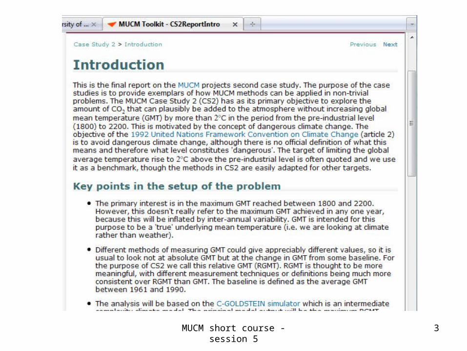
MUCM short course - session 5 3

The challenge
How much CO2 can we survive?
How much CO2 can we add to the atmosphere without increasing global mean temperature more than 2°C?
Several ambiguities in this questionObviously depends on time profile of CO2 emissions
And on time horizon
Two degrees increase relative to what?
How to define and measure global mean temperature
Even if we resolve those, how would we answer the question?
Need a simulator to predict the future
And much more besides!
MUCM short course - session 5 5
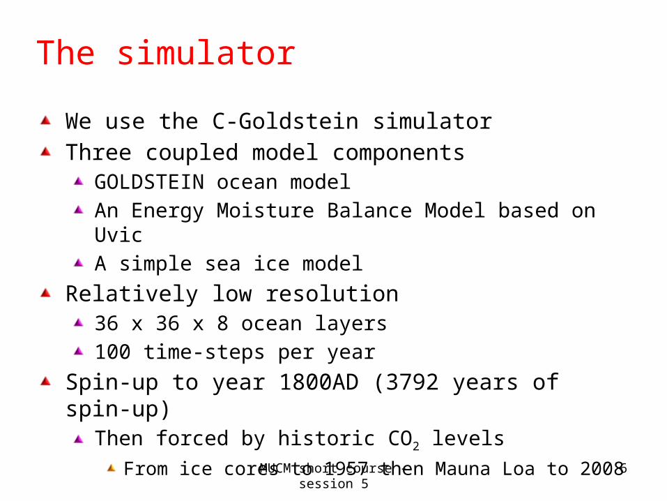
The simulator
We use the C-Goldstein simulator
Three coupled model componentsGOLDSTEIN ocean model
An Energy Moisture Balance Model based on Uvic
A simple sea ice model
Relatively low resolution36 x 36 x 8 ocean layers
100 time-steps per year
Spin-up to year 1800AD (3792 years of spin-up)Then forced by historic CO2 levels
From ice cores to 1957 then Mauna Loa to 2008
MUCM short course - session 5 6
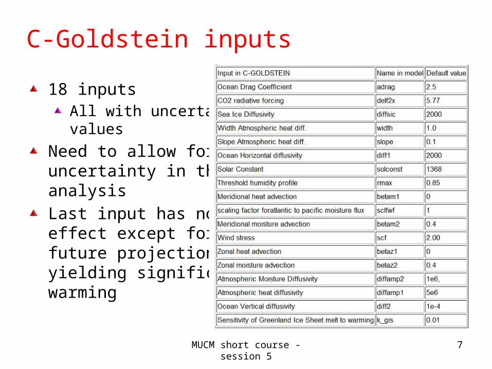
C-Goldstein inputs
18 inputsAll with uncertain values
Need to allow for uncertainty in theanalysis
Last input has no effect except for future projections yielding significant warming
MUCM short course - session 5 7
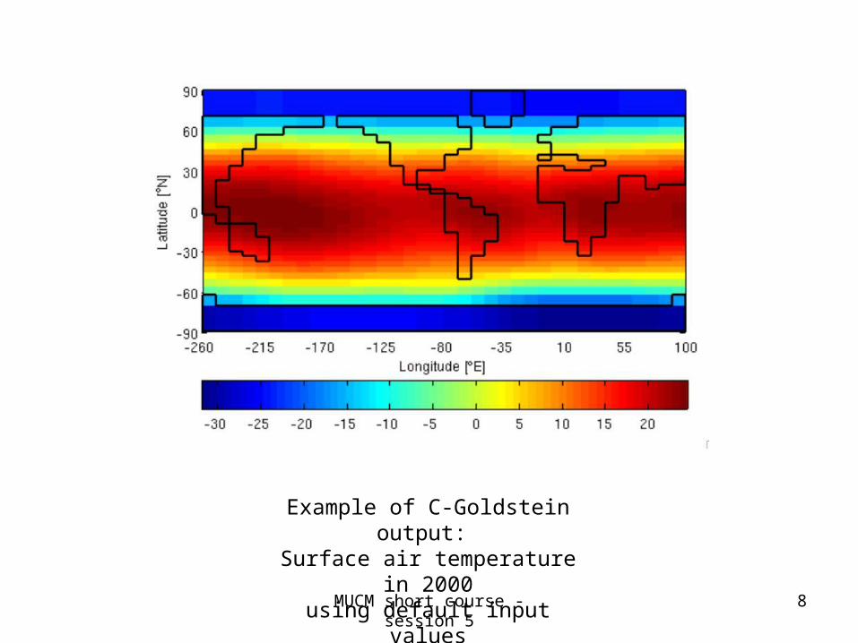
MUCM short course - session 5 8
Example of C-Goldstein output: Surface air temperature in 2000
using default input values
The data
We have historic data on global mean temperatureDecadal averages for each decade from 1850 to 2009
From HadCrut3
These are to be used to calibrate the simulatorThereby hopefully to reduce prediction uncertainty
Note that the HadCrut3 data are actually values of the temperature “anomaly”
Which brings us to the next slide
MUCM short course - session 5 9
RGMT
Two issues around defining global mean temperature (GMT)
1. Attempts to measure or model it are subject to biasesIt is generally argued that differences in GMT are more meaningful and robust
Hence our data are differences between observed GMT in a given year and the average over 1961-1990
We call this (observed) RGMTRelative GMT
The output that we take from C-Goldstein for each decade is also converted to (simulated) RGMT
By subtracting average simulator output for 1961-1990
MUCM short course - session 5 10
Weather versus climate
2. HadCrut3 data show substantial inter-annual variabilityThere is weather on top of underlying climate
C-Goldstein output is much smootherJust climate
We assessed the inter-annual error variance by fitting a smooth cubic
And looking at decadal deviations from this line
True RGMT is defined as underlying climateObserved RGMT is true RGMT plus measurement and inter-annual (weather) error
Simulated RGMT is true RGMT plus input error and model discrepancy
MUCM short course - session 5 11
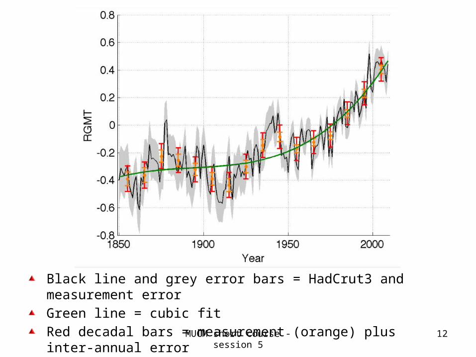
Black line and grey error bars = HadCrut3 and measurement error
Green line = cubic fit
Red decadal bars = measurement (orange) plus inter-annual errorMUCM short course - session 5 12
Target 2 degree rise
The target of keeping with 2 degrees warming was defined as
Relative to pre-industrial temperature
For future up to year 2200So max true RGMT should be less than (pre-industrial + 2)
The objective was to assess the probability of achieving this target
For given future CO2 emissions scenarios
Averaged with respect to all sources of uncertaintyAfter calibration to historic RGMT data
Including emulation uncertainty
MUCM short course - session 5 13
Elicitation
Parameter distributions
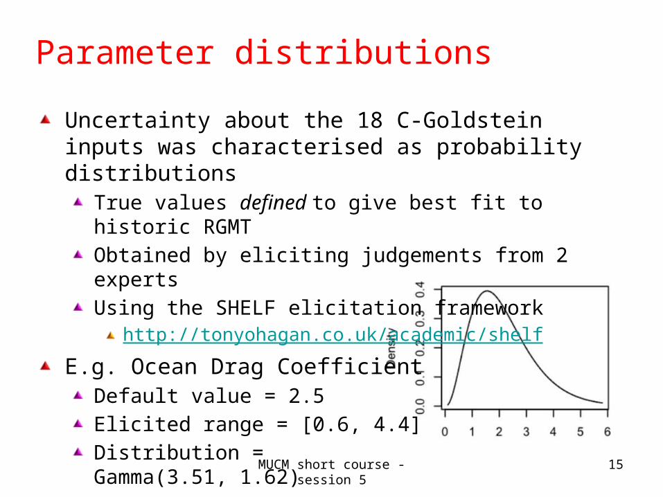
Uncertainty about the 18 C-Goldstein inputs was characterised as probability distributions
True values defined to give best fit to historic RGMT
Obtained by eliciting judgements from 2 experts
Using the SHELF elicitation frameworkhttp://tonyohagan.co.uk/academic/shelf
E.g. Ocean Drag CoefficientDefault value = 2.5
Elicited range = [0.6, 4.4]
Distribution = Gamma(3.51, 1.62)
MUCM short course - session 5 15
Model discrepancy
Beliefs about discrepancy between C-Goldstein RGMT and true RGMT also elicited
From the same two experts
Defined for true values of inputs
Predicting ahead to year 2200
Experts thought model discrepancy would grow with temperature
The higher the temperature, the further we get from where we can check the simulator against to reality
Simulator error will grow rapidly as we extrapolate
Complex and difficult elicitation exerciseDetails in toolkit
MUCM short course - session 5 16
Analysis
Two emulators
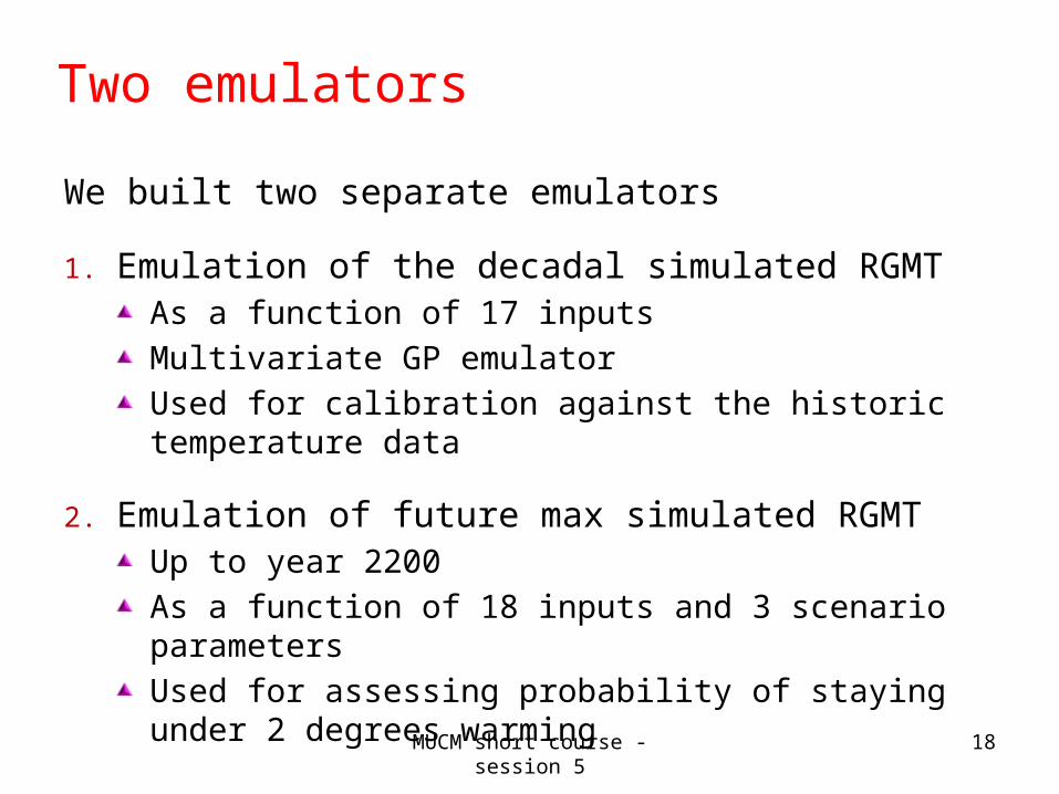
We built two separate emulators
1. Emulation of the decadal simulated RGMTAs a function of 17 inputs
Multivariate GP emulator
Used for calibration against the historic temperature data
2. Emulation of future max simulated RGMTUp to year 2200
As a function of 18 inputs and 3 scenario parameters
Used for assessing probability of staying under 2 degrees warming
MUCM short course - session 5 18
The first emulator
C-Goldstein takes about one hour to spin-up and run forward to 2008
We ran it 256 times to create a training sample
According to a complex design strategy – see the toolkit!
After removing runs where no result or implausible results were obtained, we had 204 runs
The multivariate emulator was built
And validated on a further 79 (out of 100) simulator runs
Validation was poor over the baseline period 1961-90 but otherwise good
MUCM short course - session 5 19
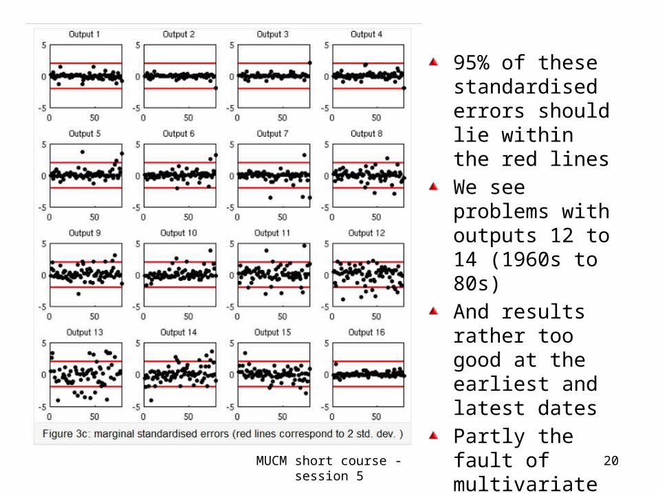
95% of these standardised errors should lie within the red lines
We see problems with outputs 12 to 14 (1960s to 80s)
And results rather too good at the earliest and latest dates
Partly the fault of multivariate GP
MUCM short course - session 5 20
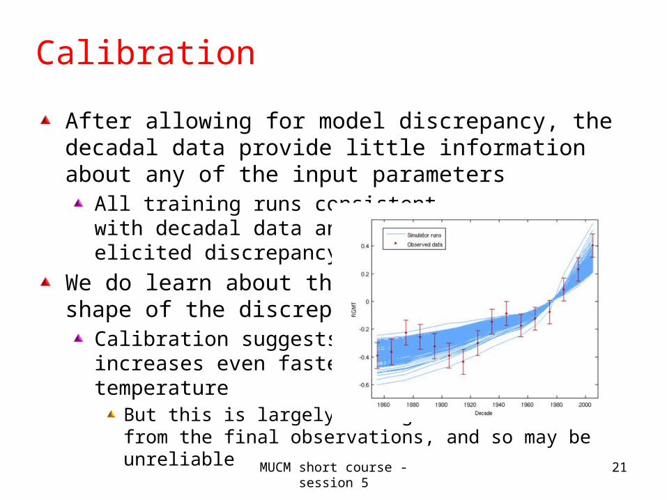
Calibration
After allowing for model discrepancy, the decadal data provide little information about any of the input parameters
All training runs consistentwith decadal data and theelicited discrepancy
We do learn about the shape of the discrepancy
Calibration suggests itincreases even faster withtemperature
But this is largely coming from the final observations, and so may be unreliable
MUCM short course - session 5 21
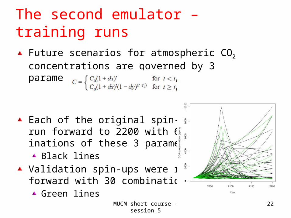
The second emulator – training runs
Future scenarios for atmospheric CO2 concentrations are governed by 3 parameters, t1, dx and dy
Each of the original spin-ups was run forward to 2200 with 64 comb-inations of these 3 parameters
Black lines
Validation spin-ups were run forward with 30 combinations
Green lines
MUCM short course - session 5 22
Computing probabilities of target
The second emulator was built for the max RGMT outputAnd validated well
Particularly well when temperature rise was smaller
Probability of true RGMT rise staying below a specific threshold
Computed by averaging emulator predicted probabilities
Averaged over the sample of calibrated parameter values
Allowing for discrepancy and emulation uncertainties
Calculation can be done for any (t1, dx, dy) and any threshold
We used 2, 4 and 6 degrees
MUCM short course - session 5 23
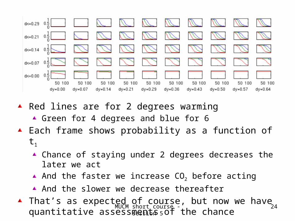
Red lines are for 2 degrees warmingGreen for 4 degrees and blue for 6
Each frame shows probability as a function of t1
Chance of staying under 2 degrees decreases the later we act
And the faster we increase CO2 before acting
And the slower we decrease thereafter
That’s as expected of course, but now we have quantitative assessments of the chance
MUCM short course - session 5 24
Conclusions
We can now see just how early and how hard we must act on CO2 emissions
In order to have a good chance of staying under 2 degrees
Lots of caveats, of courseIn particular, it’s dependent on the expert elicitation of C-Goldstein model discrepancy
We have very little data to check those judgements
But nobody has attempted to include that factor beforeThis is pioneering work!
Emulation was crucialEven for a moderate complexity model like C-Goldstein
MUCM short course - session 5 25
Recommended