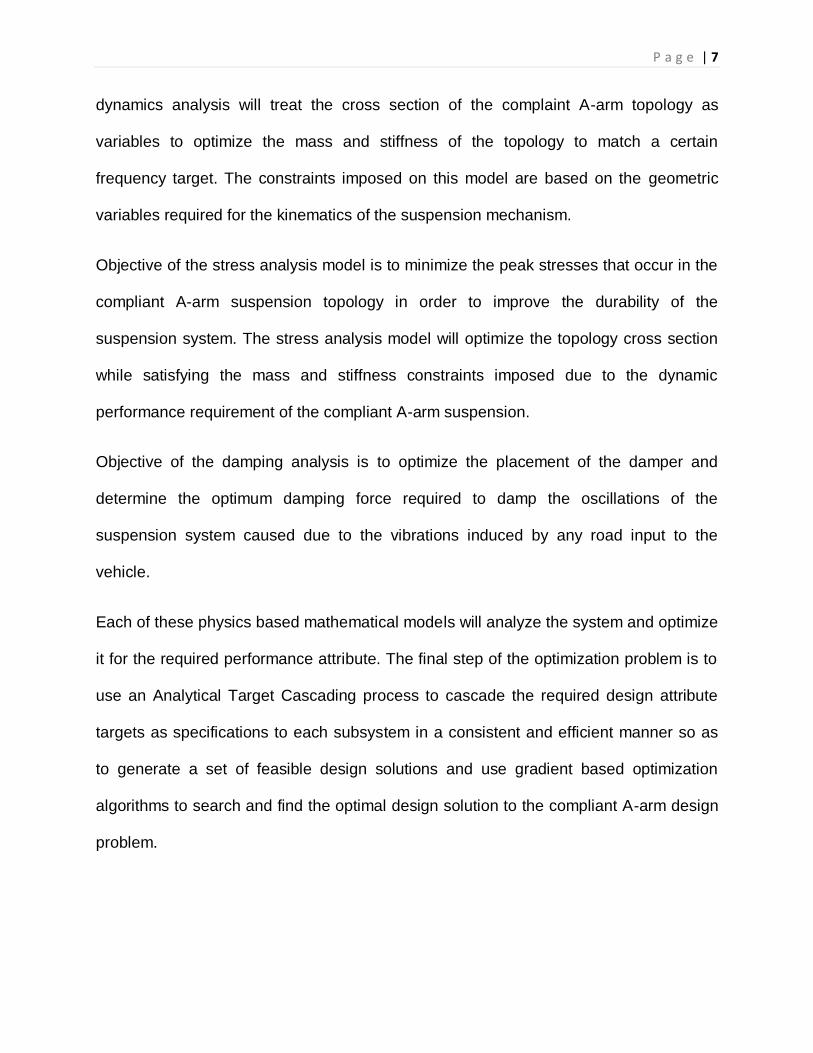
COMPLIANT SUSPENSION DESIGN OPTIMIZATION
ME-555 W08 DESIGN OPTIMIZATION PROJECT TEAM-5-FINAL REPORT
GIRISH KRISHNAN KARAN GOYAL MUKUND NEMALI ROHAN SINGH
P a g e | 2
Lc
Lh
Uaf
thetah
Uar
Laf
Lar
thetala
thetaua
alphauaf
thetab
thetat
betauaf
etauaf
Alphauar
betauar
etauar
alphalaf
betalaf
alphalar
etalaf
etalar
betalar
dc
dc1
thetah
lamdab
lamdat
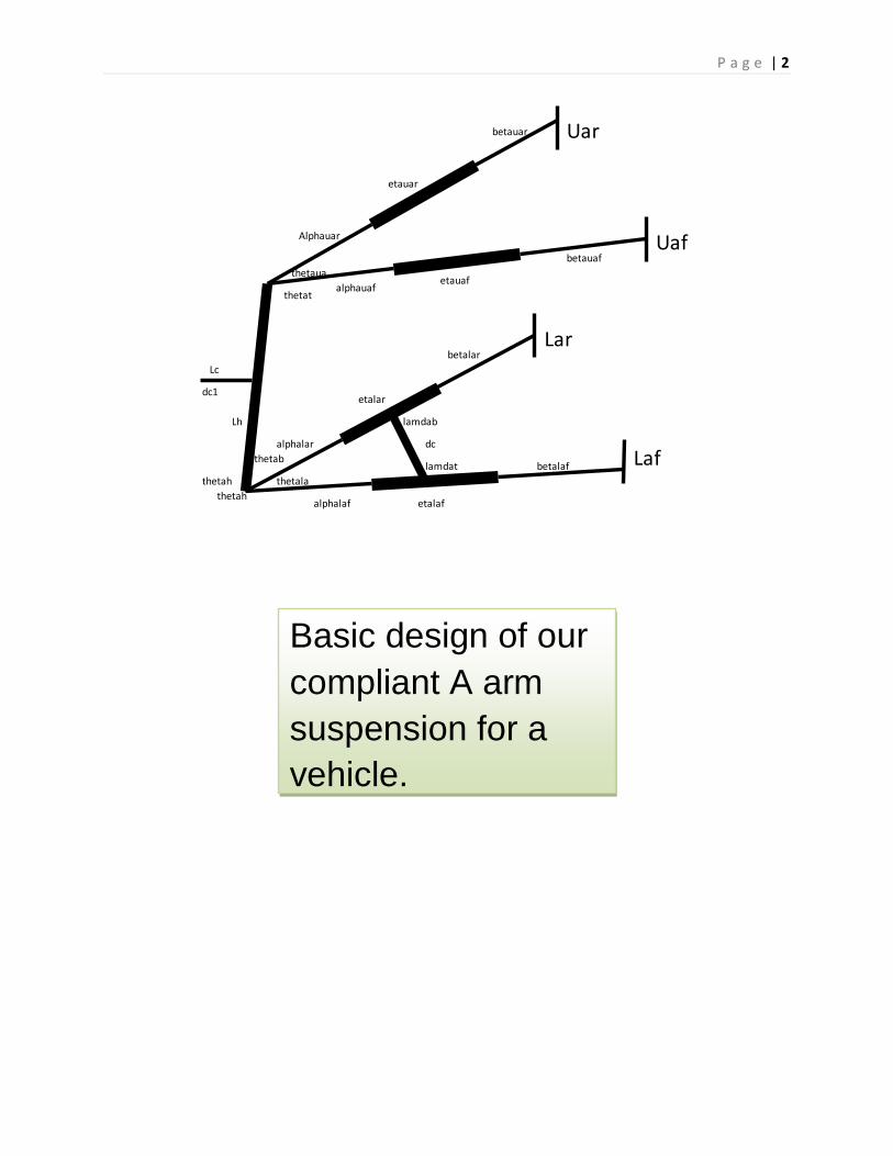
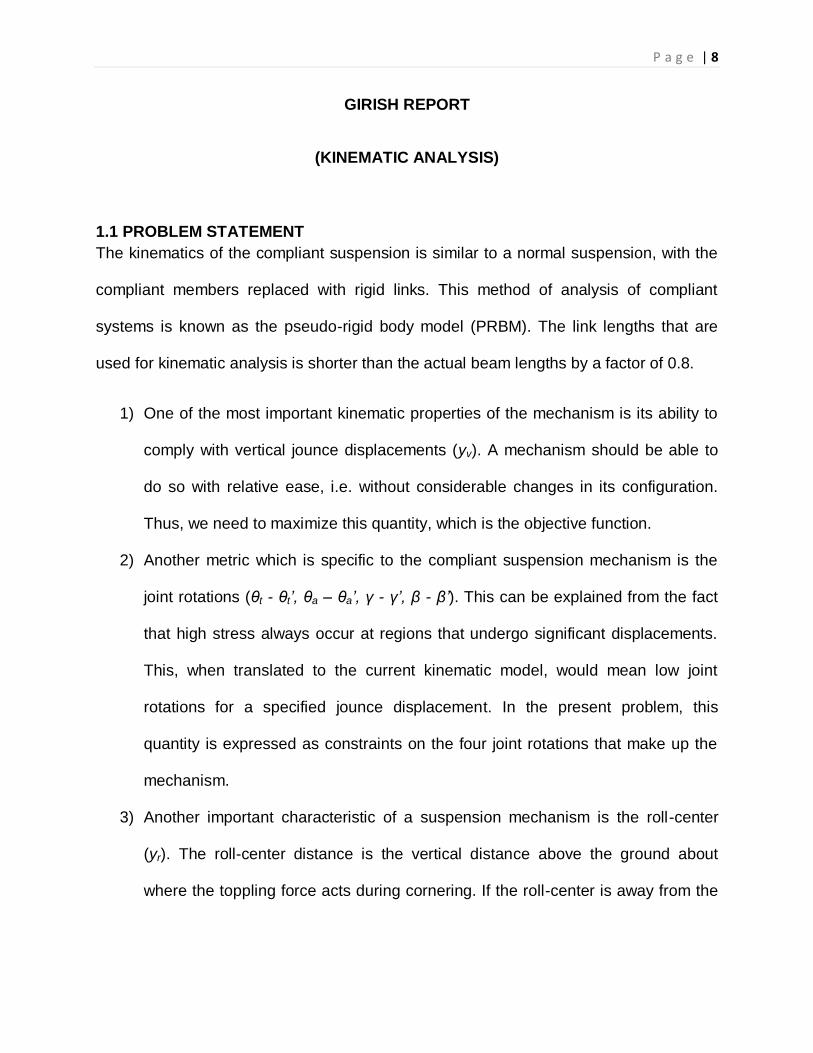
Basic design of our
compliant A arm
suspension for a
vehicle.
P a g e | 3
Contents GIRISH REPORT ................................................................................................................................. 8
(KINEMATIC ANALYSIS) .................................................................................................................... 8
1.1 PROBLEM STATEMENT .............................................................................................................. 8
1.2 NOMENCLATURE ....................................................................................................................... 11
THE VARIABLES:............................................................................................................................... 12
PARAMETERS: .................................................................................................................................. 12
1.3 MATHEMATICAL MODELS: ....................................................................................................... 14
1.4 SUMMARY MODEL: .................................................................................................................... 15
1.5 MODEL ANALYSIS: ..................................................................................................................... 15
MUKUND NEMALI (DYNAMIC ANALYSIS)..................................................................................... 20
2 PROBLEM STATEMENT ............................................................................................................... 20
2.1. MATHEMATICAL MODEL.......................................................................................................... 20
2.2. NOMENCLATURE: ..................................................................................................................... 21
2.3. SUMMARY MODEL: ................................................................................................................... 23
2.4. MODEL ANALYSIS: .................................................................................................................... 24
2.5. NUMERICAL RESULTS: ............................................................................................................ 25
ROHAN SINGH ................................................................................................................................... 29
(STRUCTURAL ANALYSIS) .............................................................................................................. 29
3.2. NOMENCLATURE: ............................................................................................................. 32
3.3. MATHEMATICAL MODEL: ................................................................................................. 33
3.4. CONSTRAINTS: .................................................................................................................. 34
3.5. SUMMARY OF THE MODEL: ............................................................................................ 37
3.6. DESIGN VARIABLES: ........................................................................................................ 38
3.7. DESIGN PARAMETERS: ................................................................................................... 38
3.8. OPTIMIZATION ANALYSIS: .............................................................................................. 39
3.9. ANALYSIS:........................................................................................................................... 46
3.10. SUBSYSTEM TRADEOFFS: .......................................................................................... 47
4. DAMPER PLACEMENT ANALYSIS ............................................................................................. 49
4.1 PROBLEM STATEMENT ............................................................................................................ 49
4.2 NOMENCLATURE: ...................................................................................................................... 51
4.3 MATHEMATICAL MODEL ........................................................................................................... 52
P a g e | 4
VARIABLES .................................................................................................................................... 53
CONSTRAINTS .............................................................................................................................. 53
PARAMETERS ............................................................................................................................... 54
4.4 SUMMARY MODEL ..................................................................................................................... 55
4.5 MODEL ANALYSIS ...................................................................................................................... 55
4.6 RESULTS...................................................................................................................................... 56
4.7 CONCLUSION & FUTURE WORK ............................................................................................. 60
FINAL SYSTEM INTEGRATION ....................................................................................................... 61
5.2. CONSTRAINTS: .......................................................................................................................... 61
5.3. FINAL SUMMARY: ...................................................................................................................... 63
5.4. OPTIMIZATION ANALYSIS: ...................................................................................................... 64
5.5. RESULT: ...................................................................................................................................... 68
5.6. FUTURE WORK: ......................................................................................................................... 69
APPENDIX IA...................................................................................................................................... 71
APPENDIX IB...................................................................................................................................... 75
APPENDIX 3A .................................................................................................................................... 77
APPENDIX 4 ....................................................................................................................................... 79
REFERENCES: .................................................................................................................................. 80
P a g e | 5
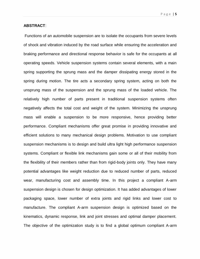
ABSTRACT:
Functions of an automobile suspension are to isolate the occupants from severe levels
of shock and vibration induced by the road surface while ensuring the acceleration and
braking performance and directional response behavior is safe for the occupants at all
operating speeds. Vehicle suspension systems contain several elements, with a main
spring supporting the sprung mass and the damper dissipating energy stored in the
spring during motion. The tire acts a secondary spring system, acting on both the
unsprung mass of the suspension and the sprung mass of the loaded vehicle. The
relatively high number of parts present in traditional suspension systems often
negatively affects the total cost and weight of the system. Minimizing the unsprung
mass will enable a suspension to be more responsive, hence providing better
performance. Compliant mechanisms offer great promise in providing innovative and
efficient solutions to many mechanical design problems. Motivation to use compliant
suspension mechanisms is to design and build ultra light high performance suspension
systems. Compliant or flexible link mechanisms gain some or all of their mobility from
the flexibility of their members rather than from rigid-body joints only. They have many
potential advantages like weight reduction due to reduced number of parts, reduced
wear, manufacturing cost and assembly time. In this project a compliant A-arm
suspension design is chosen for design optimization. It has added advantages of lower
packaging space, lower number of extra joints and rigid links and lower cost to
manufacture. The compliant A-arm suspension design is optimized based on the
kinematics, dynamic response, link and joint stresses and optimal damper placement.
The objective of the optimization study is to find a global optimum compliant A-arm
P a g e | 6
suspension design that satisfies all the prescribed constraints and meets all the
cascaded attribute targets.
INTRODUCTION:
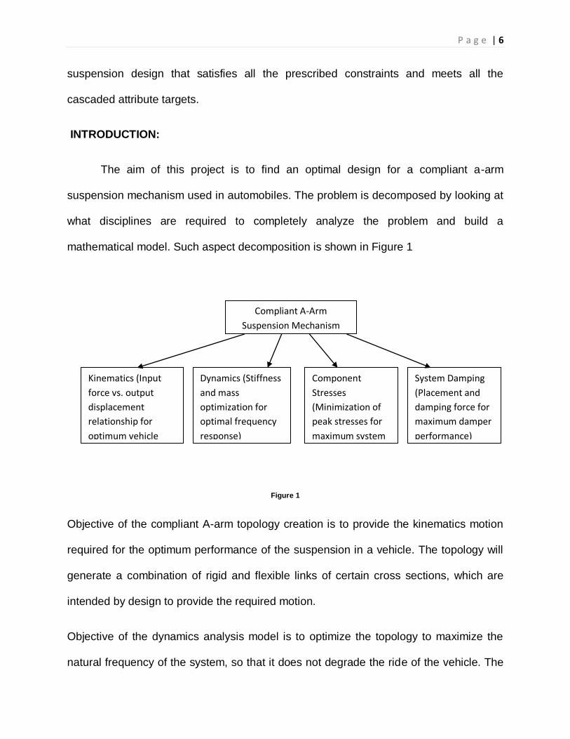
The aim of this project is to find an optimal design for a compliant a-arm
suspension mechanism used in automobiles. The problem is decomposed by looking at
what disciplines are required to completely analyze the problem and build a
mathematical model. Such aspect decomposition is shown in Figure 1
Figure 1
Objective of the compliant A-arm topology creation is to provide the kinematics motion
required for the optimum performance of the suspension in a vehicle. The topology will
generate a combination of rigid and flexible links of certain cross sections, which are
intended by design to provide the required motion.
Objective of the dynamics analysis model is to optimize the topology to maximize the
natural frequency of the system, so that it does not degrade the ride of the vehicle. The
Compliant A-Arm
Suspension Mechanism
Design
Kinematics (Input
force vs. output
displacement
relationship for
optimum vehicle
ride and handling
Dynamics (Stiffness
and mass
optimization for
optimal frequency
response)
Component
Stresses
(Minimization of
peak stresses for
maximum system
durability
System Damping
(Placement and
damping force for
maximum damper
performance)
P a g e | 7
dynamics analysis will treat the cross section of the complaint A-arm topology as
variables to optimize the mass and stiffness of the topology to match a certain
frequency target. The constraints imposed on this model are based on the geometric
variables required for the kinematics of the suspension mechanism.
Objective of the stress analysis model is to minimize the peak stresses that occur in the
compliant A-arm suspension topology in order to improve the durability of the
suspension system. The stress analysis model will optimize the topology cross section
while satisfying the mass and stiffness constraints imposed due to the dynamic
performance requirement of the compliant A-arm suspension.
Objective of the damping analysis is to optimize the placement of the damper and
determine the optimum damping force required to damp the oscillations of the
suspension system caused due to the vibrations induced by any road input to the
vehicle.
Each of these physics based mathematical models will analyze the system and optimize
it for the required performance attribute. The final step of the optimization problem is to
use an Analytical Target Cascading process to cascade the required design attribute
targets as specifications to each subsystem in a consistent and efficient manner so as
to generate a set of feasible design solutions and use gradient based optimization
algorithms to search and find the optimal design solution to the compliant A-arm design
problem.
P a g e | 8
GIRISH REPORT
(KINEMATIC ANALYSIS)
1.1 PROBLEM STATEMENT
The kinematics of the compliant suspension is similar to a normal suspension, with the
compliant members replaced with rigid links. This method of analysis of compliant
systems is known as the pseudo-rigid body model (PRBM). The link lengths that are
used for kinematic analysis is shorter than the actual beam lengths by a factor of 0.8.
1) One of the most important kinematic properties of the mechanism is its ability to
comply with vertical jounce displacements (yv). A mechanism should be able to
do so with relative ease, i.e. without considerable changes in its configuration.
Thus, we need to maximize this quantity, which is the objective function.
2) Another metric which is specific to the compliant suspension mechanism is the
joint rotations (θt - θt’, θa – θa’, γ - γ’, β - β’). This can be explained from the fact
that high stress always occur at regions that undergo significant displacements.
This, when translated to the current kinematic model, would mean low joint
rotations for a specified jounce displacement. In the present problem, this
quantity is expressed as constraints on the four joint rotations that make up the
mechanism.
3) Another important characteristic of a suspension mechanism is the roll-center
(yr). The roll-center distance is the vertical distance above the ground about
where the toppling force acts during cornering. If the roll-center is away from the
P a g e | 9
center of gravity of the vehicle, there will be moments, which cause the vehicle to
overturn.
4) The vertical jounce of the mechanism (yv) should move almost in a straight
vertical line. In reality it moves along an arc of the circle. It is of our interest to
increase the radius of travel. The instantaneous center of circle of the arc (xin)
traversed by the wheel needs to be maximized to make it move along a straight
line.
5) The link lengths and the angles ( l1 , l2, l3, l4 and θ1, θt, θh, θa ) which together
form the variables of which define a configuration of the four-bar mechanism are
the variables for the present problem. To put together a four-bar mechanism with
these variables, we need to satisfy the triangle inequality condition with certain
link lengths. These inequalities add a set of three further constraints.
6) Furthermore it should be realized that a four-bar mechanism‟s configuration is
completely dependent on which of the link lengths is shorter than the other. First
of all the link lengths should be such that they satisfy the Grashoff‟s criterion,
which can make a four-bar mechanism possible from a given set of link lengths
and angles. The Grashoff‟s criterion cannot be explicitly put into the model as
constraints because there may be some point in the middle of iterations when the
constraints can get temporarily violated. This is why we need to put bounds on
the link lengths such that Grashoff‟s criterion is always satisfied.
P a g e | 10
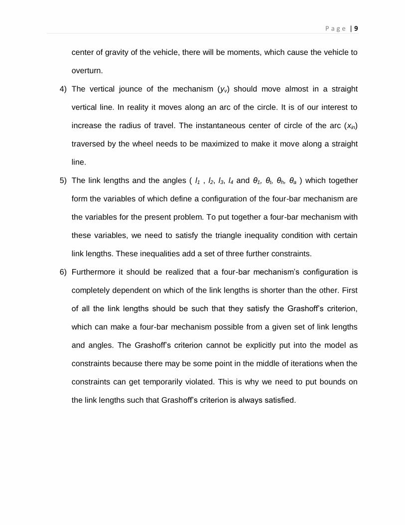
Figure 1.1.
Different configurations of a four-bar mechanism , ‘s’ is the smallest link, l is the largest
and p and q are intermediate links.
Shown in Fig. 1.1 are all the four configurations that a four-bar mechanism can take. Of
these only certain types of configurations can be suitable for the suspension. Choice a,
where the fixed link is the shortest link, is a good choice because large angles of
rotation with relatively straight line motion for link p is obtained. Option b also allows
large angles of rotation but is limited because the largest link rotates significantly for
large angles of rotations of links s and p. Option c is not suitable because large crank
angles almost intersect p and l. This situation must be avoided, and can be done so by
making sure that the connecting link is not the shortest. Finally, option d is the best
suited since it gives a pure straight line motion, however, it will be seen later that such a
design has a very bad roll-center height.
Ideally, we have to avoid case ‘c’ and parts of case ‘b’ and case ‘a’ where there
are large variations in the link lengths, leading to large rotations of the connecting link to
which the wheel is to be attached.
a b c d
P a g e | 11
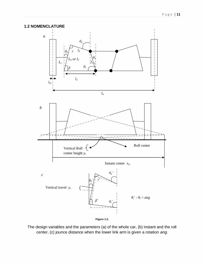
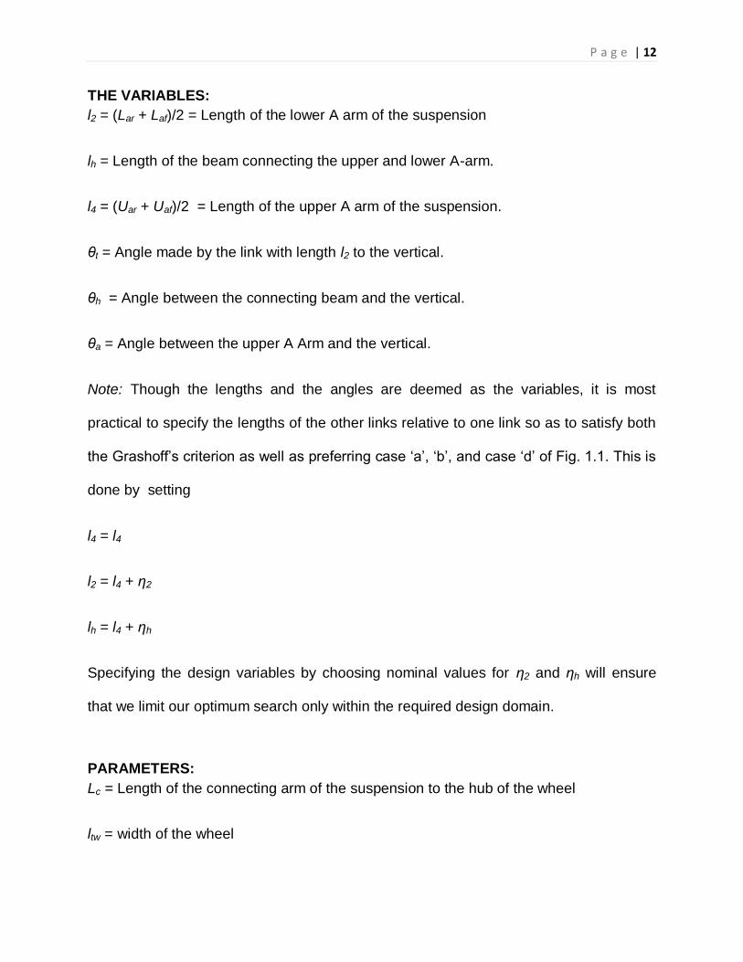
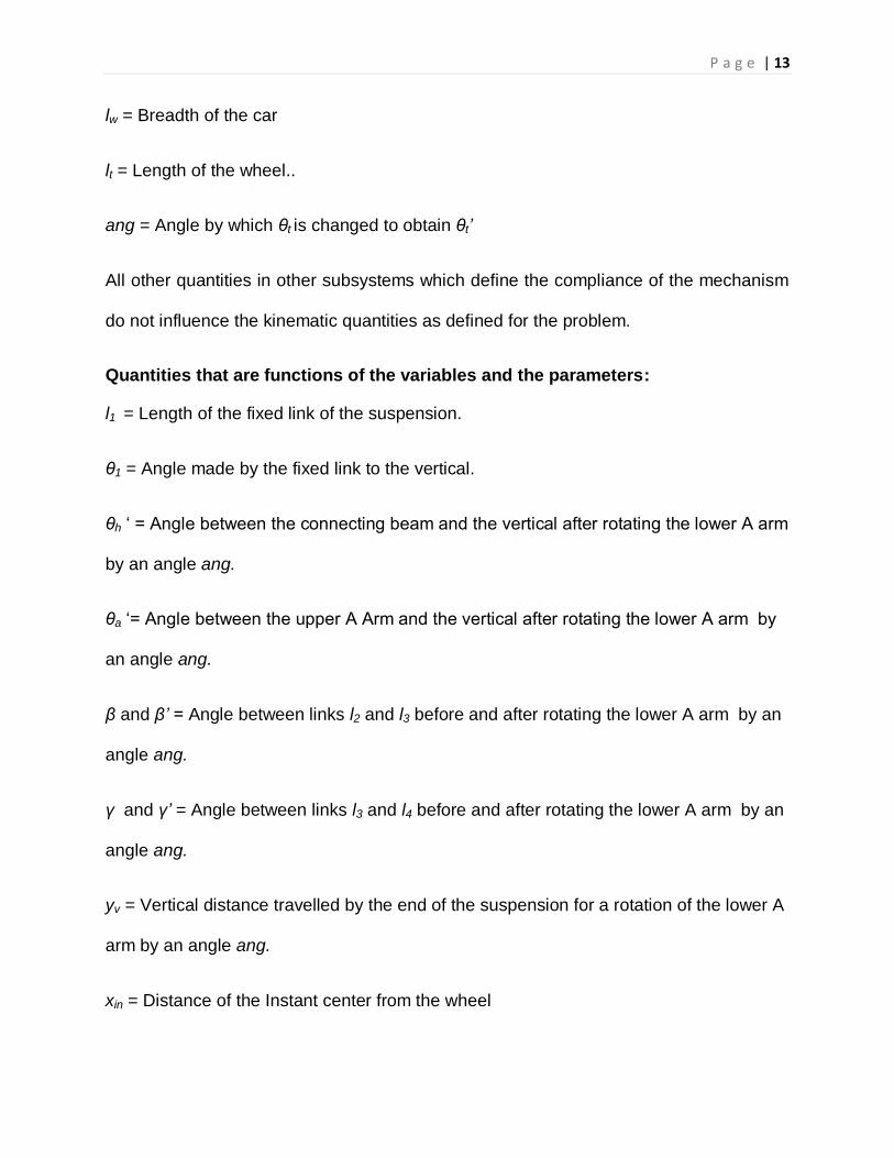
1.2 NOMENCLATURE
Figure 1.2.
The design variables and the parameters (a) of the whole car, (b) instant and the roll
center, (c) jounce distance when the lower link arm is given a rotation ang.
lw
ltw
l1
l2
Lh or l3
l4
θt
θ1
θa
θh
Lc
Roll center
Instant center xin
Vertical Roll
center height yr
θh’
θa’
θt’
Vertical travel yv
β
γ
β'
γ'
a
b
c
θt’ - θt ≈ ang
P a g e | 12
THE VARIABLES:
l2 = (Lar + Laf)/2 = Length of the lower A arm of the suspension
lh = Length of the beam connecting the upper and lower A-arm.
l4 = (Uar + Uaf)/2 = Length of the upper A arm of the suspension.
θt = Angle made by the link with length l2 to the vertical.
θh = Angle between the connecting beam and the vertical.
θa = Angle between the upper A Arm and the vertical.
Note: Though the lengths and the angles are deemed as the variables, it is most
practical to specify the lengths of the other links relative to one link so as to satisfy both
the Grashoff‟s criterion as well as preferring case „a‟, „b‟, and case „d‟ of Fig. 1.1. This is
done by setting
l4 = l4
l2 = l4 + η2
lh = l4 + ηh
Specifying the design variables by choosing nominal values for η2 and ηh will ensure
that we limit our optimum search only within the required design domain.
PARAMETERS:
Lc = Length of the connecting arm of the suspension to the hub of the wheel
ltw = width of the wheel
P a g e | 13
lw = Breadth of the car
lt = Length of the wheel..
ang = Angle by which θt is changed to obtain θt’
All other quantities in other subsystems which define the compliance of the mechanism
do not influence the kinematic quantities as defined for the problem.
Quantities that are functions of the variables and the parameters:
l1 = Length of the fixed link of the suspension.
θ1 = Angle made by the fixed link to the vertical.
θh „ = Angle between the connecting beam and the vertical after rotating the lower A arm
by an angle ang.
θa „= Angle between the upper A Arm and the vertical after rotating the lower A arm by
an angle ang.
β and β’ = Angle between links l2 and l3 before and after rotating the lower A arm by an
angle ang.
γ and γ’ = Angle between links l3 and l4 before and after rotating the lower A arm by an
angle ang.
yv = Vertical distance travelled by the end of the suspension for a rotation of the lower A
arm by an angle ang.
xin = Distance of the Instant center from the wheel
P a g e | 14
yin = Distance of the roll-center from the vertical.
Note: All the lengths here are normalized with half the width of the car, i.e. lw/2.
1.3 MATHEMATICAL MODELS:
We have mathematical formulation for all the quantities used for the objective functions
and constraints as defined in the problem statement. The detailed expressions of the
model are given in Appendix I.
To evaluate the jounce distance yv, we increase the lower arm angle from θ to θ’, such
that θ - θ’ is ang. All the other angle changes are evaluated in Appendix I. These
angles should not exceed the input angle ang, and if they do, it leads to large stresses
in the flexures that make up the compliant mechanism.
The instant center is the center about which the wheel rotates instantly when it
encounters some jounce. To maintain perfect straight line motion, the instant center
should be at infinity, ideally. Furthermore the roll-center is the point about which the
cornering forces act when the vehicle takes a turn. The roll center is measured here
from the ground and it is given by a very simple relation, which includes the instant
center as
2 in w
r
in
y ly
x Eq 1.1
This shows that once the width of the car with which all the lengths are normalized with
is fixed, the roll center is inversely proportional to the instant center distance from one
end of the wheel and is its value completely determines the roll-center height. Thus, the
roll-center height and the instant center height cannot be independently imposed as two
P a g e | 15
independent constraints. Thus, in the present problem only constraint on the roll-center
is imposed.
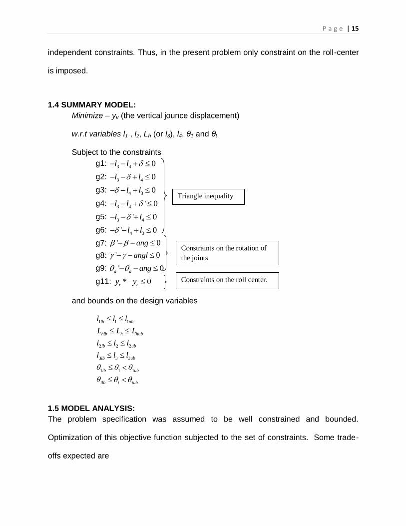
1.4 SUMMARY MODEL:
Minimize – yv (the vertical jounce displacement)
w.r.t variables l1 , l2, Lh (or l3), l4, θ1 and θt
Subject to the constraints
g1: 3 4 0l l
g2: 3 4 0l l
g3: 4 3 0l l
g4: 3 4 ' 0l l
g5: 3 4' 0l l
g6: 4 3' 0l l
g7: ' 0ang
g8: ' 0angl
g9: ' 0a a ang
g11: * 0r ry y
and bounds on the design variables
1 1 1
2 2 2
3 3 3
1 1 1
lb ub
hlb h hub
lb ub
lb ub
lb ub
tlb t tub
l l l
L L L
l l l
l l l
1.5 MODEL ANALYSIS:
The problem specification was assumed to be well constrained and bounded.
Optimization of this objective function subjected to the set of constraints. Some trade-
offs expected are
Triangle inequality
Constraints on the rotation of
the joints
Constraints on the roll center.
P a g e | 16
1) Angles of link rotations and the vertical jounce: These tend to make the links as
close to the configuration in Fig. 1.1c as possible as making the links
perpendicular to each other is the only way we can achieve a high vertical jounce
for limited angles of link rotations.
2) Roll center: Having a high roll-center would require from Eq. 1.1 a small instant
center, which instantly conflicts with the angle and the jounce requirements.
Otherwise, no monotonicity analysis can be directly seen from the expressions as they
are highly convoluted and nonlinear. This means that more about this model could be
revealed from optimization alone. Optimization was carried out using the Sequential
Quadratic Programming algorithm in the MATLAB‟s optimization toolbox. The necessary
parameter values for the problem are shown below.
Lc = Length of the connecting arm of the suspension to the hub of the wheel =0.2 lw
ltw = width of the wheel = 0.1lw
lw = Breadth of the car =1
lt = Length of the wheel.= 0.8 lw
ang = Angle by which θt is changed to obtain θt’ = π/20
yr = The roll-center height = lw/4.
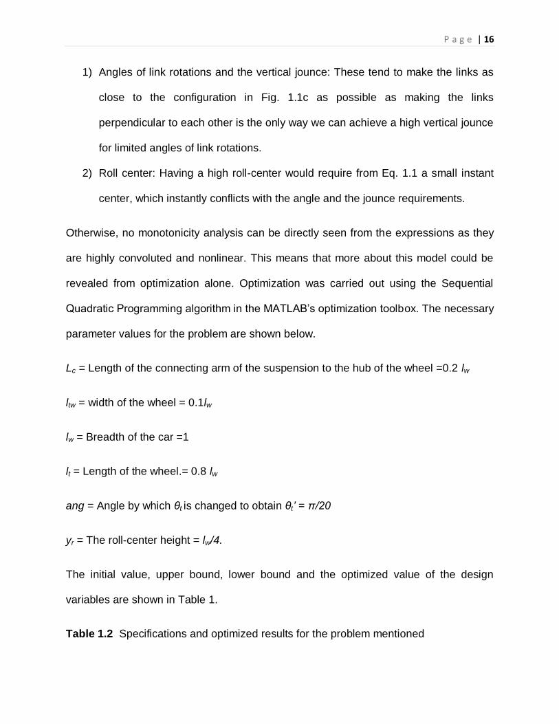
The initial value, upper bound, lower bound and the optimized value of the design
variables are shown in Table 1.
Table 1.2 Specifications and optimized results for the problem mentioned
P a g e | 17
l4 η2= l4 - l2 ηh =lh - l4 θt θh θa
Initial value
0.1 0.3 0.3 10*pi/180 10*pi/180 -10*pi/180
Upper bound
1.2 1 0.9 20*pi/180 20*pi/180 20*pi/180
Lower bound
0 0 0 -20*pi/180 -20*pi/180 -20*pi/180
Optimized value
0.1797 0 0.9 20*pi/180 -20*pi/180 -2.61*pi/180
Figure 1.3
The initial and final configuration of the four-bar mechanism
The algorithm convergence details are given in the appendix. Some of the key features
of the result given by the algorithm are
1) The initial jounce travel was 0.060332 units (normalized with respect to the width
of the car). The final jounce travel was around 0.217668 units. This is an
improvement close to 300%.
2) The intermediate link length lh went to the upper bound along with the angle θt.
The angle θh went to the lower bound.
ltw
l1
l2
Lh or l3
l4
θt
θ1
θa
θh
Lc
β
γ
Initial mechanism
configuration
Optimized
mechanism
P a g e | 18
3) Two constraints, one bounding the angle of rotation of link l4 and the roll-center
constraints were active. The Lagrange multipliers corresponding to these
constraints were found to be positive.
4) The hessian was found to be positive definite.
5) The optimized results were independent of the initial guess indicating
some sort of a localized convexity within the range of the problem.
The lengthening of the links was evident from the problem specifications because that is
the only way that one can get large displacements for small link rotation angles. Thus
the optimized solution is in sync with intuition.
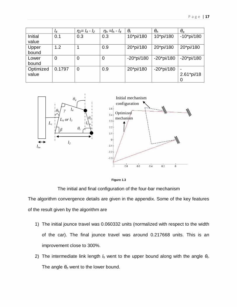
The constraint history is shown in the next page with the function evaluations
Figure 1.4.
Convergence history of the algorithm
The only parameter worth varying in this problem is the value of the roll-center
constraint. This is shown in Table 1.2.
P a g e | 19
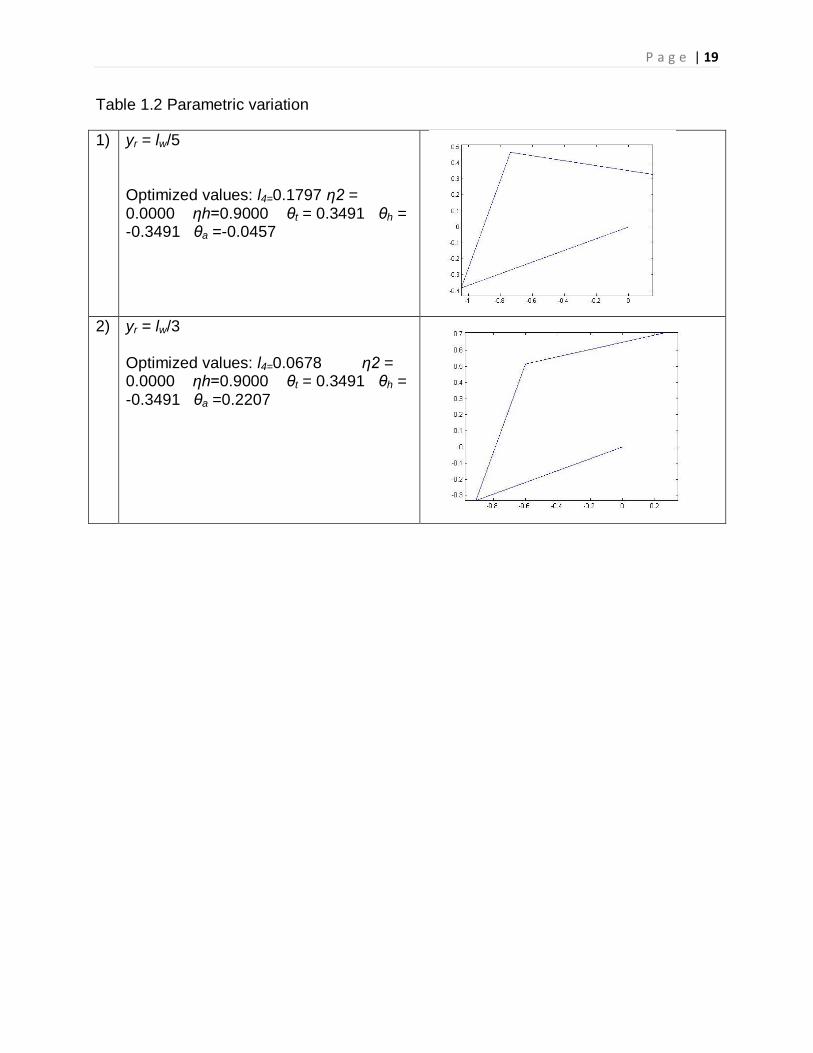
Table 1.2 Parametric variation
1) yr = lw/5 Optimized values: l4=0.1797 η2 = 0.0000 ηh=0.9000 θt = 0.3491 θh = -0.3491 θa =-0.0457
2) yr = lw/3
Optimized values: l4=0.0678 η2 = 0.0000 ηh=0.9000 θt = 0.3491 θh = -0.3491 θa =0.2207
P a g e | 20
MUKUND NEMALI (DYNAMIC ANALYSIS)
2 PROBLEM STATEMENT: The dynamics analysis model is developed to study the
dynamic performance of the compliant A-arm topology. The objective of this analysis is
to maximize the natural frequency of the suspension mechanism so as not to cause
degradation in ride or cause any unwanted NVH characteristic. The suspension
mechanism will have a fundamental frequency mode and other higher multiple modes of
vibration. The interest here is in the first natural frequency mode.
2.1. MATHEMATICAL MODEL:
Maximize Natural Frequency ( i ) of the suspension topology
Maximize i in 0 ii XMKXF
Subject to:
ul
uil
lonv
latv
vv
G
AAAG
KKG
KKG
KKG
2,1
*
:5
:4
10:3
10:2
:1
Objective function is a matrix equation relating the mass and stiffness of the suspension
topology expressed as an Eigen value equation to solve for the system natural
frequencies. Though the problem solution will have multiple Eigen values (natural
frequencies) that satisfy the equation, the interest in this problem is to maximize the first
mode natural frequency.
P a g e | 21
Constraint G1 establishes an upper bound on the vertical stiffness in the suspension.
The vertical stiffness is required to be low in order for the suspension to be flexible in
the vertical direction. This is because in a compliant suspension the kinematics is
achieved by the elasticity in the structure. The vertical stiffness is also required to be
high in order to maximize the natural frequency of the suspension in order to have good
vehicle ride characteristics. The vertical stiffness has conflicting requirements.
Constraint G2 establishes a constraint on the lateral stiffness in terms of the vertical
stiffness. The lateral stiffness has to be greater than 10 times the vertical stiffness for
good handling. The longitudinal stiffness has to be higher for better energy absorption
during acceleration and braking.
Constraint G3 establishes a constraint on the longitudinal stiffness in terms of the
vertical stiffness. The longitudinal stiffness has to be greater than 10 times the vertical
stiffness for better straight line performance during acceleration and braking.
Constraints G4 and G5 establish bounds on the geometric variables of the suspension
design.
2.2. NOMENCLATURE:
K – Stiffness of the suspension mechanism in N/mm
M – Mass of the suspension mechanism in kg
E – Young's Modulus in N/mm2
- Density of the beam material
P a g e | 22
i - Natural frequencies of the suspension mechanism in Hz
Kv – Vertical Stiffness in N/mm
Kv* - Target Vertical Stiffness in N/mm
Klat – Lateral Stiffness in N/mm
Klon – Longitudinal Stiffness in N/mm
Al – Lower limit for beam cross section area in mm2
Au – Upper limit for beam cross section area in mm2
Ai – Cross section area of each beam element in mm2
l - Lower limit of the angle between the two legs of the A-arm in Deg
u - Upper limit of the angle between the two legs of the A-arm in Deg
1 - Angle between the two legs of the upper A-arm in Rad
2 - Angle between the two legs of the lower A-arm in Rad
The cross section area Ai and angle are variables in the optimization algorithm and
the stiffness values (Kv, Klat, Klon) and mass values M are parameters, whose values do
not change in a particular run of the optimization algorithm. Parametric study was
conducted for different values of stiffness, mass and elasticity.
P a g e | 23
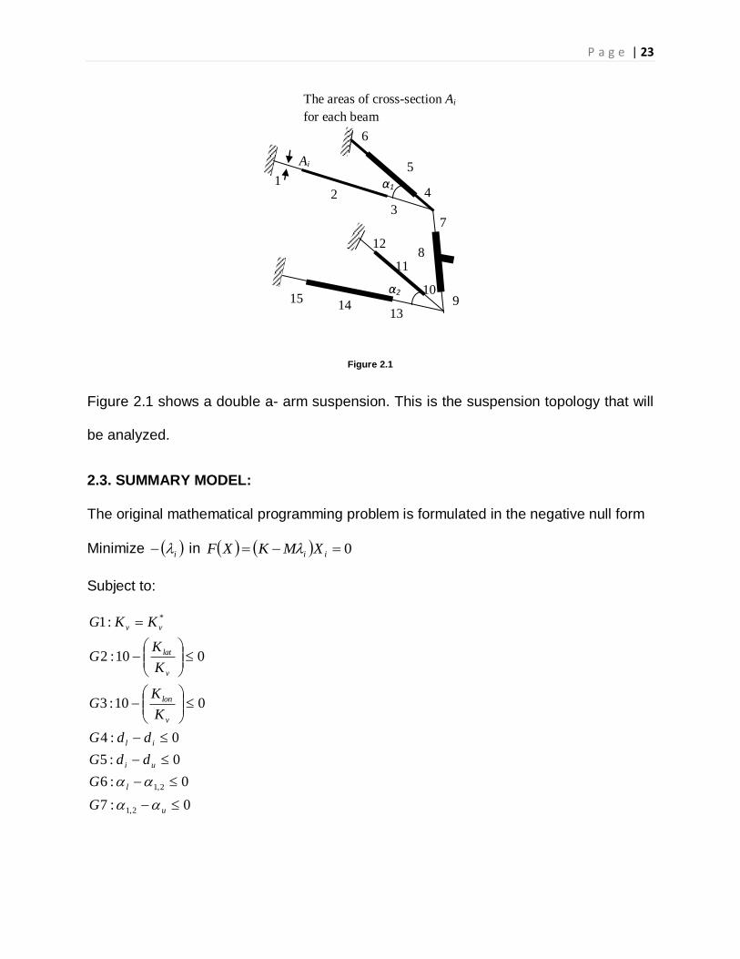
Figure 2.1
Figure 2.1 shows a double a- arm suspension. This is the suspension topology that will
be analyzed.
2.3. SUMMARY MODEL:
The original mathematical programming problem is formulated in the negative null form
Minimize i in 0 ii XMKXF
Subject to:
0:7
0:6
0:5
0:4
010:3
010:2
:1
2,1
2,1
*
u
l
ui
il
v
lon
v
lat
vv
G
G
ddG
ddG
K
KG
K
KG
KKG
Ai
The areas of cross-section Ai
for each beam
1 2
3
4
5
6
7
8
9 10
11
12
13 14
15
α1
α2
P a g e | 24
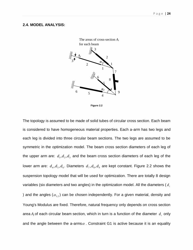
2.4. MODEL ANALYSIS:
Figure 2.2
The topology is assumed to be made of solid tubes of circular cross section. Each beam
is considered to have homogeneous material properties. Each a-arm has two legs and
each leg is divided into three circular beam sections. The two legs are assumed to be
symmetric in the optimization model. The beam cross section diameters of each leg of
the upper arm are: 321 ,, ddd and the beam cross section diameters of each leg of the
lower arm are: 654 ,, ddd . Diameters 987 ,, ddd are kept constant. Figure 2.2 shows the
suspension topology model that will be used for optimization. There are totally 8 design
variables (six diameters and two angles) in the optimization model. All the diameters ( id
) and the angles ( 2,1 ) can be chosen independently. For a given material, density and
Young's Modulus are fixed. Therefore, natural frequency only depends on cross section
area iA of each circular beam section, which in turn is a function of the diameter id only
and the angle between the a-arms . Constraint G1 is active because it is an equality
Ai
The areas of cross-section Ai
for each beam
3 2
1
1
2
3
7
8
9 4
5
6
4 5
6
α1
α2
P a g e | 25
constraint. Constraints G2 and G3 are active because they are given in terms of vK and
bound the maximum value of the stiffness from above. Stiffness values are given as
parameters in the simulation. Constraints G4 and G5are bounds on the diameters of
each beam cross section. The diameters are bounded from above and below.
Constraints G6 and G7 are bounds on the angles between the legs of the upper arm
and the lower arm. The angles are bound from above and below. The objective of the
constrained optimization problem is to optimize the cross section diameters and a-arm
angles to maximize the first mode of the natural frequency.
2.5. NUMERICAL RESULTS:
The optimization was run in MATLAB using the medium scale constrained optimization
algorithm. This algorithm uses Sequential Quadratic Programming with line search to
solve the optimization problem.
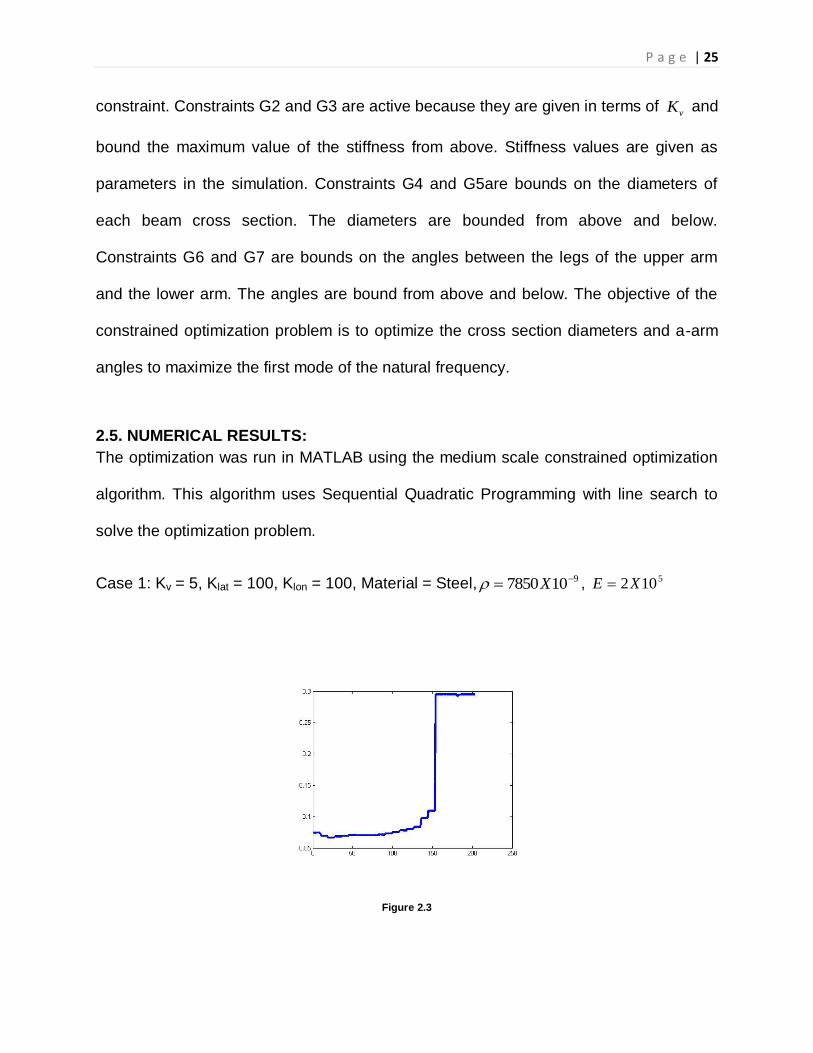
Case 1: Kv = 5, Klat = 100, Klon = 100, Material = Steel, 9107850 X , 5102XE
Figure 2.3
P a g e | 26
In the first simulation the maximum number of iterations was set to 20. The algorithm
terminated because the maximum number of iterations was reached. Figure 2.3 shows
that the natural frequency keeps increasing and started to stabilize after about 200
iterations. However, since the algorithm terminated no conclusion can be made about
the convergence of the objective function and the optimum value.
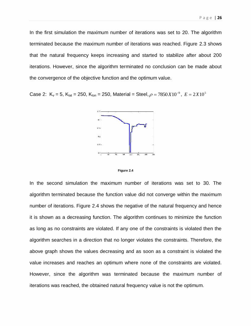
Case 2: Kv = 5, Klat = 250, Klon = 250, Material = Steel, 9107850 X , 5102XE
Figure 2.4
In the second simulation the maximum number of iterations was set to 30. The
algorithm terminated because the function value did not converge within the maximum
number of iterations. Figure 2.4 shows the negative of the natural frequency and hence
it is shown as a decreasing function. The algorithm continues to minimize the function
as long as no constraints are violated. If any one of the constraints is violated then the
algorithm searches in a direction that no longer violates the constraints. Therefore, the
above graph shows the values decreasing and as soon as a constraint is violated the
value increases and reaches an optimum where none of the constraints are violated.
However, since the algorithm was terminated because the maximum number of
iterations was reached, the obtained natural frequency value is not the optimum.
P a g e | 27
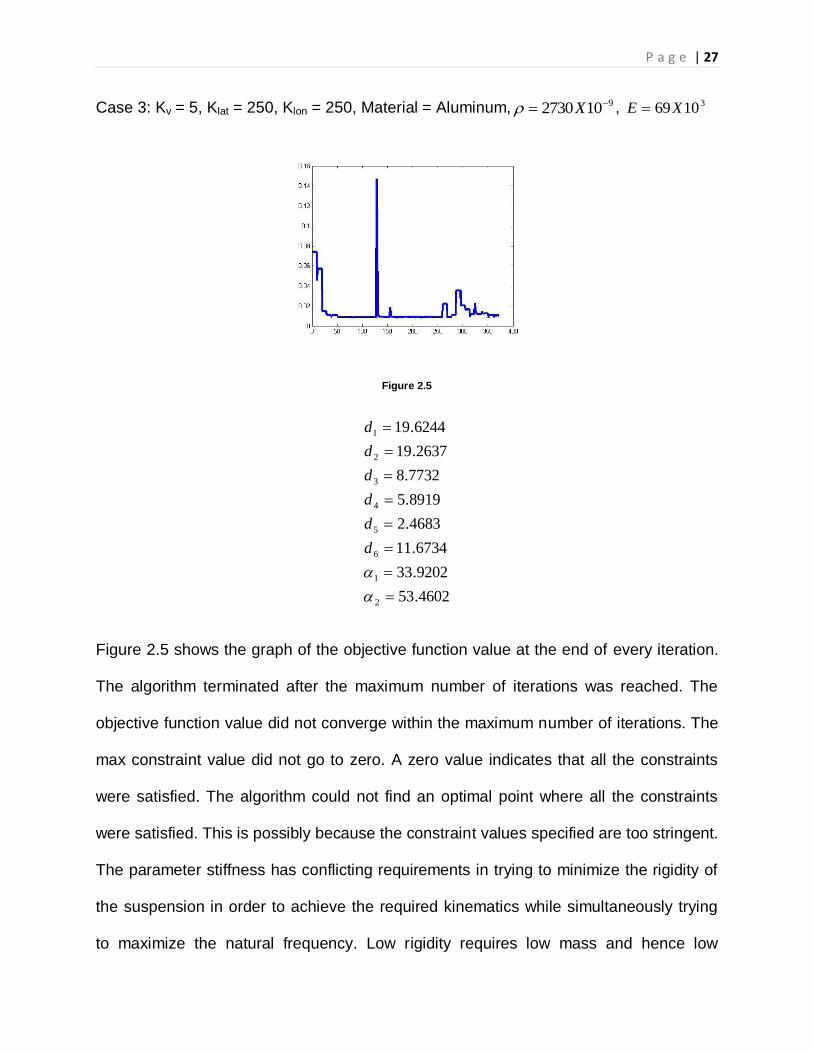
Case 3: Kv = 5, Klat = 250, Klon = 250, Material = Aluminum, 9102730 X , 31069XE
Figure 2.5
4602.53
9202.33
6734.11
4683.2
8919.5
7732.8
2637.19
6244.19
2
1
6
5
4
3
2
1
d
d
d
d
d
d
Figure 2.5 shows the graph of the objective function value at the end of every iteration.
The algorithm terminated after the maximum number of iterations was reached. The
objective function value did not converge within the maximum number of iterations. The
max constraint value did not go to zero. A zero value indicates that all the constraints
were satisfied. The algorithm could not find an optimal point where all the constraints
were satisfied. This is possibly because the constraint values specified are too stringent.
The parameter stiffness has conflicting requirements in trying to minimize the rigidity of
the suspension in order to achieve the required kinematics while simultaneously trying
to maximize the natural frequency. Low rigidity requires low mass and hence low
P a g e | 28
stiffness and high natural frequency requires high stiffness for a given mass of the
suspension. The lack of an optimal solution suggests that it is very difficult to achieve
this trade off in a real vehicle suspension and therefore a compliant suspension is not
feasible in a real vehicle. It is only applicable to small scale and light weight
applications.
P a g e | 29
ROHAN SINGH
(STRUCTURAL ANALYSIS)
3.1. PROBLEM STATEMENT:
As stated in the introduction to the report, the A-arm compliant suspension system is
attached to the chassis of the vehicle at four different points. The suspension
mechanism‟s main purpose is to absorb the energy from the shocks and impulses that
act on the vehicle from the road and various driving conditions. In doing so the
suspension is acted upon by a large number of forces, moments and torques in different
directions. The range of loads that act upon the suspension can be very large from a
minor bump to a bump in a large pothole which can create high amount of impact
stresses. These loads will create a large amount of stress in the beams of the A-arm
mechanism. Since this suspension system is a compliant mechanism, made up of semi
rigid compliant beams (Euler beams), the stresses created by these forces can be very
large and may exceed the yield strength of the A-arm beams. This would prove to be
disastrous for the vehicle as it could have fatal results. Thus the main aim of my sub
system optimization is to reduce or minimize the maximum stress that occurs in the
complaint suspension and thus keep the stress levels in the beams below the yield
stress levels and make sure they have a high fatigue life.
The various forces, moments and torques that can act on the suspension from the
various road and driving conditions are listed below:
P a g e | 30
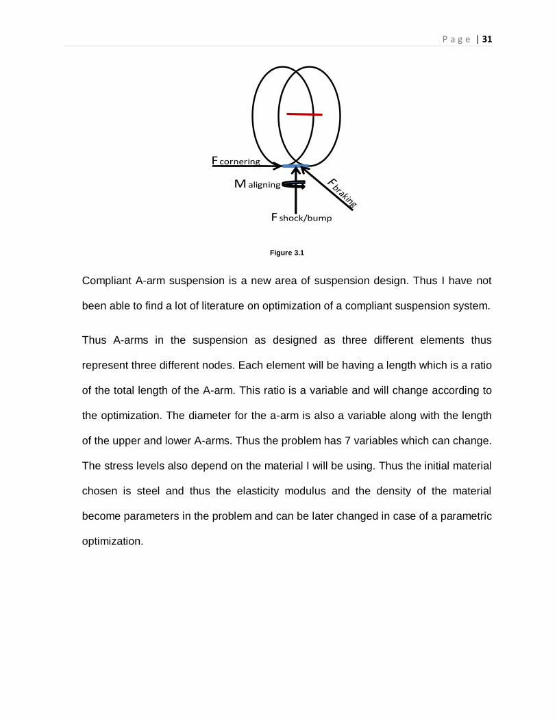
3.1.1 Vertical impulse force: the force that acts on the wheel when it bumps into a
pothole or goes over rough terrain. This causes a large amount of impulse
force, most of which is absorbed by the suspension. In doing so a large
amount of stress is created in the beams to absorb these forces. These
forces act in the vertical direction denoted by the positive Z direction.
3.1.2. Braking/Traction forces: the forces acting on the suspension system by the
traction provided to the wheel by the engine or the braking forces that are
acted upon by the brakes onto the wheel. These forces act in the longitudinal
direction which is denoted by the positive Y direction.
3.1.3. Cornering forces: these are the forces experienced by the wheel/suspension
during the cornering of the vehicle. Cornering leads to large amount of forces
acting in the lateral direction, denoted by the positive X direction.
3.1.4. Aligning torque: aligning torque is caused due to the self aligning property of
the wheel to center itself automatically after a turn. This causes an aligning
moment around the positive Y direction.
The direction of various forces acting on the wheel/suspension is indicated in the
figure on the next page.
P a g e | 31
Figure 3.1
Compliant A-arm suspension is a new area of suspension design. Thus I have not
been able to find a lot of literature on optimization of a compliant suspension system.
Thus A-arms in the suspension as designed as three different elements thus
represent three different nodes. Each element will be having a length which is a ratio
of the total length of the A-arm. This ratio is a variable and will change according to
the optimization. The diameter for the a-arm is also a variable along with the length
of the upper and lower A-arms. Thus the problem has 7 variables which can change.
The stress levels also depend on the material I will be using. Thus the initial material
chosen is steel and thus the elasticity modulus and the density of the material
become parameters in the problem and can be later changed in case of a parametric
optimization.
M aligning
F shock/bump
F cornering
P a g e | 32
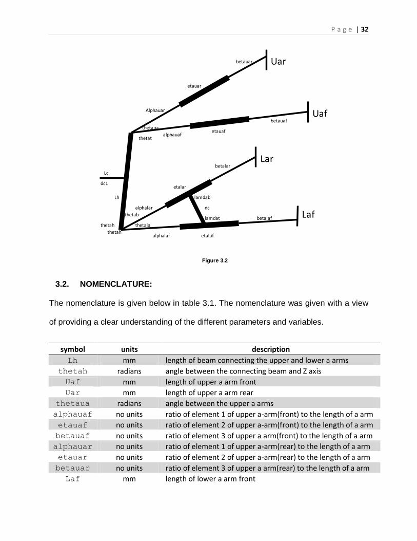
Figure 3.2
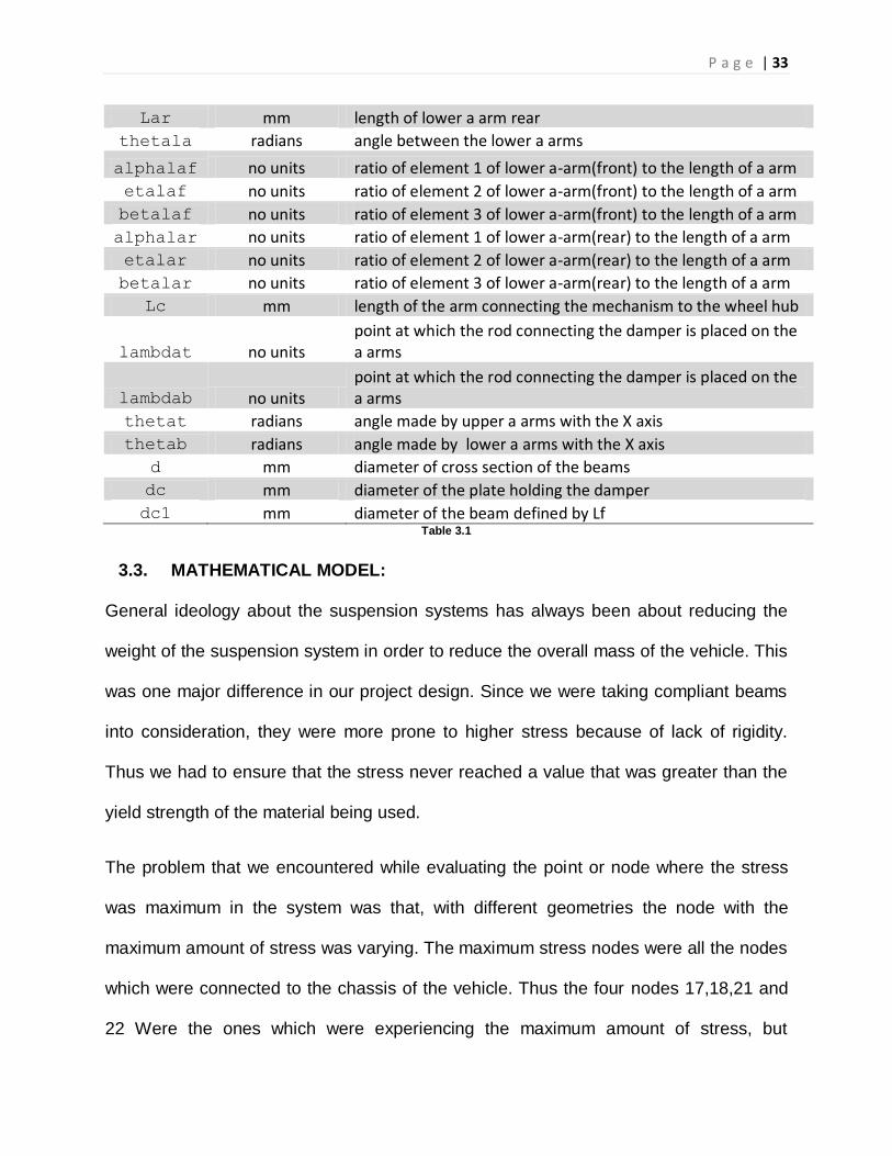
3.2. NOMENCLATURE:
The nomenclature is given below in table 3.1. The nomenclature was given with a view
of providing a clear understanding of the different parameters and variables.
symbol units description
Lh mm length of beam connecting the upper and lower a arms
thetah radians angle between the connecting beam and Z axis
Uaf mm length of upper a arm front
Uar mm length of upper a arm rear
thetaua radians angle between the upper a arms
alphauaf no units ratio of element 1 of upper a-arm(front) to the length of a arm
etauaf no units ratio of element 2 of upper a-arm(front) to the length of a arm
betauaf no units ratio of element 3 of upper a arm(front) to the length of a arm
alphauar no units ratio of element 1 of upper a-arm(rear) to the length of a arm
etauar no units ratio of element 2 of upper a-arm(rear) to the length of a arm
betauar no units ratio of element 3 of upper a arm(rear) to the length of a arm
Laf mm length of lower a arm front
Lc
Lh
Uaf
thetah
Uar
Laf
Lar
thetala
thetaua
alphauaf
thetab
thetat
betauaf
etauaf
Alphauar
betauar
etauar
alphalaf
betalaf
alphalar
etalaf
etalar
betalar
dc
dc1
thetah
lamdab
lamdat
P a g e | 33
Lar mm length of lower a arm rear
thetala radians angle between the lower a arms
alphalaf no units ratio of element 1 of lower a-arm(front) to the length of a arm
etalaf no units ratio of element 2 of lower a-arm(front) to the length of a arm
betalaf no units ratio of element 3 of lower a-arm(front) to the length of a arm
alphalar no units ratio of element 1 of lower a-arm(rear) to the length of a arm
etalar no units ratio of element 2 of lower a-arm(rear) to the length of a arm
betalar no units ratio of element 3 of lower a-arm(rear) to the length of a arm
Lc mm length of the arm connecting the mechanism to the wheel hub
lambdat no units point at which the rod connecting the damper is placed on the a arms
lambdab no units point at which the rod connecting the damper is placed on the a arms
thetat radians angle made by upper a arms with the X axis
thetab radians angle made by lower a arms with the X axis
d mm diameter of cross section of the beams
dc mm diameter of the plate holding the damper
dc1 mm diameter of the beam defined by Lf Table 3.1
3.3. MATHEMATICAL MODEL:
General ideology about the suspension systems has always been about reducing the
weight of the suspension system in order to reduce the overall mass of the vehicle. This
was one major difference in our project design. Since we were taking compliant beams
into consideration, they were more prone to higher stress because of lack of rigidity.
Thus we had to ensure that the stress never reached a value that was greater than the
yield strength of the material being used.
The problem that we encountered while evaluating the point or node where the stress
was maximum in the system was that, with different geometries the node with the
maximum amount of stress was varying. The maximum stress nodes were all the nodes
which were connected to the chassis of the vehicle. Thus the four nodes 17,18,21 and
22 Were the ones which were experiencing the maximum amount of stress, but
P a g e | 34
depending on the length of the a arms, the angle between them, the different ratios of
the elements the maximum stress was varying from one node to the other. Thus to
overcome this problem I took the maximum value of stress at each of the nodes in every
iteration and then tried to minimize the stress at that particular node. Thus this formed
the main objective function of the problem.
Zav= ([abs (Z18), abs (Z17), abs (Z22), abs (Z21)]) Yav= ([abs (Y18), abs (Y17), abs (Y22), abs (Y21)])
Objective function= Stress=max (Zav+Yav)
3.4. CONSTRAINTS:
Thus there were varying set of constraints that had to be enforced on the system.
Let us begin with the first and most important of constraints.
3.4.1. Jounce of the suspension: the main objective of the function is to absorb the
bumps and provide passenger comfort. This is accomplished by the spring
damper system in the suspension which makes the suspension to move in
the vertical direction and thus absorbs the various road and engine inputs.
Thus the greater distance it moves the better it absorbs the energy of the
bumps. But due to space requirements and vehicle design, it cannot have a
large value of deflection. Thus it has limit on the maximum deflection of the
wheel. This is basically to stop the wheel from bottoming out. Another
important factor that was required for the suspension was that it had to
absorb a certain amount of energy to provide passenger ride comfort. Thus
for the different range of forces that it was subjected to it had to deflect by a
P a g e | 35
certain amount in the Z direction to absorb the energy of the bump. Thus
another constraint had to be added, requiring that it had to deflect by a certain
minimum amount in the vertical or Z direction to provide the required
passenger comfort level. This deflection was determined by assuming certain
stiffness for the vehicle and thus calculating the deflection based on that. The
constraint was thus given by
G1:w1-jmax<=0 G2:=jmin-w1
In the above equation w1 gives the displacement of node 2 in the vertical z direction.
The jounce travel jmax and jmin were determined by the available space and the
minimum stiffness requirement for the suspension.
3.4.2. The various forces as shown in figure 1.1 cause a lot of deflection in various
directions which cause unwanted effects in the suspension mechanism. The
cornering force causes a moment about the X axis which causes a rotation
about the y axis thus changing the camber angle. The camber angle plays an
important role in the handling of the vehicle, thus changes in it causes a
negative effect for the vehicles handling. Thus this camber angle change had
to be kept to a minimum. The constraint for this is given by:
G3: (x4+x1)-cambmin<=0
Here the points x1 and x4 give the deflection in the X direction for nodes 1 and
4. Cambmin indicates the minimum camber angle change allowed for the
vehicle.
3.4.3. The braking force causes a displacement in the longitudinal Y direction and
also causes a moment around the vertical Z axis. The moment by the aligning
P a g e | 36
torque also causes a rotation about the vertical Z axis. This rotation causes
the steering angle to change which is undesirable for the vehicle. Thus a
constraint had to be placed on the allowable rotation for the steering angle.
The constraint is given by:
G4: thz3-stirmin<=0
The thz3 represents the change in angle about the Z direction of node 3. The
stirmin value for the suspension was given as half a degree.
3.4.4. Since there were forces acting in the longitudinal direction, I had to bind the
movement of the node 2 in the longitudinal direction, such that it didn‟t
displace greater than a certain amount, thereby causing slipping of the wheel.
G5: uy2-longdpmax<=0
The term uy2 is the deflection caused in the Y axis at node 2. The
Longdpmax was selected on the basis of the suspension having stiffness
which was very high compared to the stiffness in the vertical(Z) direction but not
being infinitely rigid.
3.4.5. One of the main things in any vehicle is to reduce the mass of the vehicle in
order to improve the efficiency and the performance of the vehicle. The
suspension system has to be light in order for the overall vehicle weight to be
light as well as it reduces the unsprung weight of the vehicle which improves
the ride and handling of the vehicle. Thus a constraint had to be added to
bind the upper weight restriction on the suspension system. The constraint
was given by:
G6: Mass-massmin<=0
P a g e | 37
The mass in the above equation indicates the sum of the individual masses of
the beams. The massmin is given by the current weight of a similar rigid
suspension system.
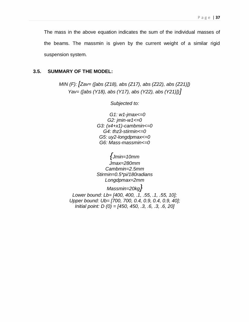
3.5. SUMMARY OF THE MODEL:
MIN (F): [Zav= ([abs (Z18), abs (Z17), abs (Z22), abs (Z21)])
Yav= ([abs (Y18), abs (Y17), abs (Y22), abs (Y21)])]
Subjected to:
G1: w1-jmax<=0 G2: jmin-w1<=0
G3: (x4+x1)-cambmin<=0 G4: thz3-stirmin<=0
G5: uy2-longdpmax<=0 G6: Mass-massmin<=0
{Jmin=10mm
Jmax=280mm Cambmin=2.5mm
Stirmin=0.5*pi/180radians Longdpmax=2mm
Massmin=20kg} Lower bound: Lb= [400, 400, .1, .55, .1, .55, 10];
Upper bound: Ub= [700, 700, 0.4, 0.9, 0.4, 0.9, 40]; Initial point: D (0) = [450, 450, .3, .6, .3, .6, 20]
P a g e | 38
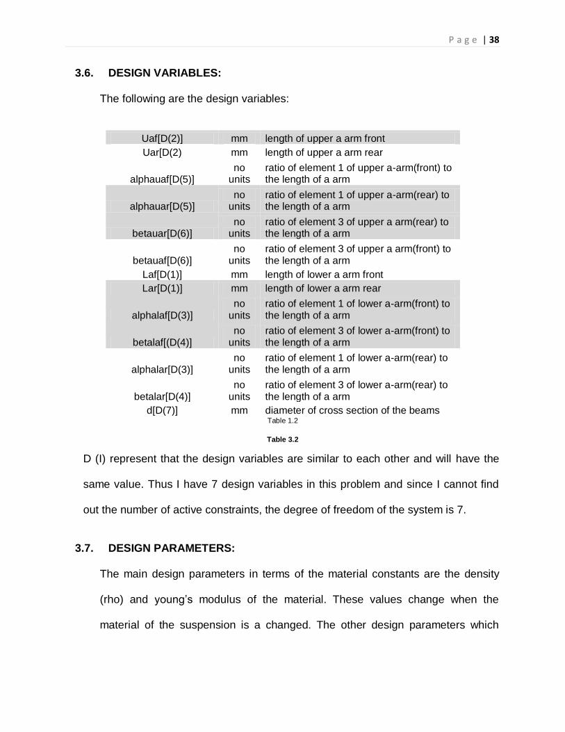
3.6. DESIGN VARIABLES:
The following are the design variables:
Uaf[D(2)] mm length of upper a arm front
Uar[D(2) mm length of upper a arm rear
alphauaf[D(5)] no
units ratio of element 1 of upper a-arm(front) to the length of a arm
alphauar[D(5)] no
units ratio of element 1 of upper a-arm(rear) to the length of a arm
betauar[D(6)] no
units ratio of element 3 of upper a arm(rear) to the length of a arm
betauaf[D(6)] no
units ratio of element 3 of upper a arm(front) to the length of a arm
Laf[D(1)] mm length of lower a arm front
Lar[D(1)] mm length of lower a arm rear
alphalaf[D(3)] no
units ratio of element 1 of lower a-arm(front) to the length of a arm
betalaf[(D(4)] no
units ratio of element 3 of lower a-arm(front) to the length of a arm
alphalar[D(3)] no
units ratio of element 1 of lower a-arm(rear) to the length of a arm
betalar[D(4)] no
units ratio of element 3 of lower a-arm(rear) to the length of a arm
d[D(7)] mm diameter of cross section of the beams Table 1.2
Table 3.2
D (I) represent that the design variables are similar to each other and will have the
same value. Thus I have 7 design variables in this problem and since I cannot find
out the number of active constraints, the degree of freedom of the system is 7.
3.7. DESIGN PARAMETERS:
The main design parameters in terms of the material constants are the density
(rho) and young‟s modulus of the material. These values change when the
material of the suspension is a changed. The other design parameters which
P a g e | 39
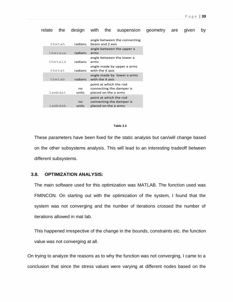
relate the design with the suspension geometry are given by
Table 3.3
These parameters have been fixed for the static analysis but can/will change based
on the other subsystems analysis. This will lead to an interesting tradeoff between
different subsystems.
3.8. OPTIMIZATION ANALYSIS:
The main software used for this optimization was MATLAB. The function used was
FMINCON. On starting out with the optimization of the system, I found that the
system was not converging and the number of iterations crossed the number of
iterations allowed in mat lab.
This happened irrespective of the change in the bounds, constraints etc. the function
value was not converging at all.
On trying to analyze the reasons as to why the function was not converging, I came to a
conclusion that since the stress values were varying at different nodes based on the
thetah radians angle between the connecting beam and Z axis
thetaua radians angle between the upper a arms
thetala radians angle between the lower a arms
thetat radians angle made by upper a arms with the X axis
thetab radians angle made by lower a arms with the X axis
lambdat
no units
point at which the rod connecting the damper is placed on the a arms
lambdab
no units
point at which the rod connecting the damper is placed on the a arms
P a g e | 40
different geometries it came up with using different iterations; it could be that the
objective function was not differentiable at some points in the domain. This could be
because the value of the maximum stress which could change from one node to
another based on the geometry of the suspension at any iteration could make the
function highly discontinuous. This could lead to the function not converging, even
though I had double checked the values of the constraints and the bounds and the
forces that were acting upon it. This was confirmed by the fact that the function was not
converging even when all the constraints were relaxed except constraints 1 and 2. This
made me sure that the function was not continuous at every point in the domain. This
was the result of the optimization for a given initial point. This was the case that
happened with every initial point that was taken into the consideration. Another fact
could also be that I had too less constraints and more variables, thus this could also be
another factor in the optimization not working.
This gave rise to a new problem of how to optimize the structural aspect of the
subsystem. In order for the function to structurally stable and be able to take the various
loads acting on the vehicle, the stress at any point could not exceed the yield stress.
Since I was sure that the maximum stress was occurring at one of the four extreme
nodes, which was confirmed by the initial analysis of the suspension system. I decided
to put a stress constraint at those nodes and came up with four constraints that bound
the stress at those nodes from above.
3.4.6. The maximum stress acting at any node in the system has to be less than the
yield strength of the material. Thus on analyses of the suspension system we
P a g e | 41
found that the maximum stresses were occurring at the four nodes 17,18,22
and 21, thus we have to have an upper bound at those four nodes and limit
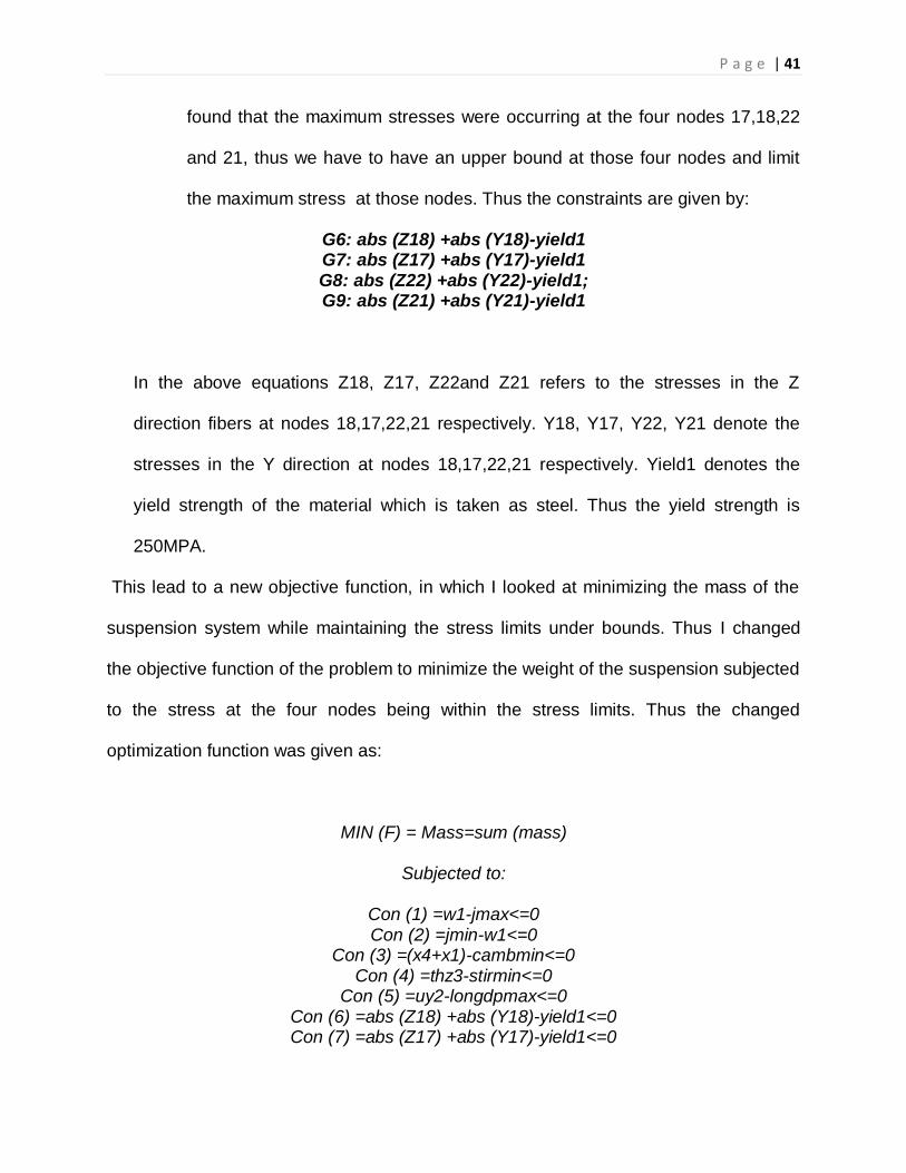
the maximum stress at those nodes. Thus the constraints are given by:
G6: abs (Z18) +abs (Y18)-yield1 G7: abs (Z17) +abs (Y17)-yield1 G8: abs (Z22) +abs (Y22)-yield1; G9: abs (Z21) +abs (Y21)-yield1
In the above equations Z18, Z17, Z22and Z21 refers to the stresses in the Z
direction fibers at nodes 18,17,22,21 respectively. Y18, Y17, Y22, Y21 denote the
stresses in the Y direction at nodes 18,17,22,21 respectively. Yield1 denotes the
yield strength of the material which is taken as steel. Thus the yield strength is
250MPA.
This lead to a new objective function, in which I looked at minimizing the mass of the
suspension system while maintaining the stress limits under bounds. Thus I changed
the objective function of the problem to minimize the weight of the suspension subjected
to the stress at the four nodes being within the stress limits. Thus the changed
optimization function was given as:
MIN (F) = Mass=sum (mass)
Subjected to:
Con (1) =w1-jmax<=0 Con (2) =jmin-w1<=0
Con (3) =(x4+x1)-cambmin<=0 Con (4) =thz3-stirmin<=0
Con (5) =uy2-longdpmax<=0 Con (6) =abs (Z18) +abs (Y18)-yield1<=0 Con (7) =abs (Z17) +abs (Y17)-yield1<=0
P a g e | 42
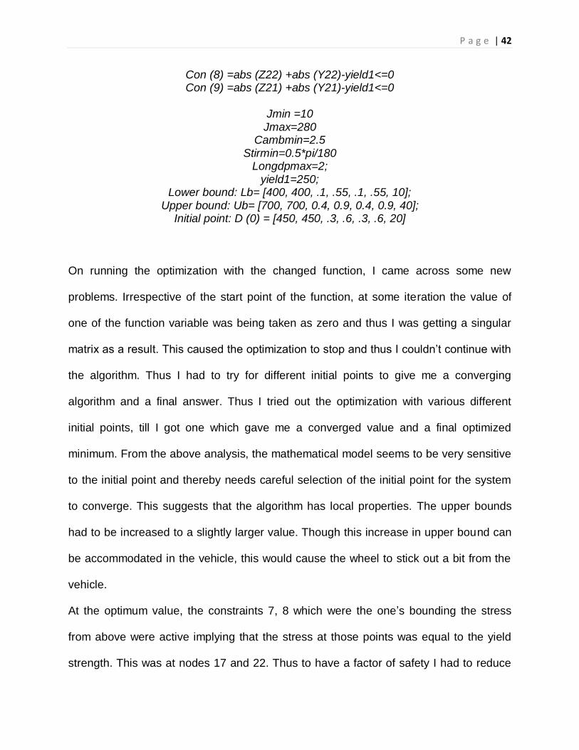
Con (8) =abs (Z22) +abs (Y22)-yield1<=0 Con (9) =abs (Z21) +abs (Y21)-yield1<=0
Jmin =10
Jmax=280 Cambmin=2.5
Stirmin=0.5*pi/180 Longdpmax=2;
yield1=250; Lower bound: Lb= [400, 400, .1, .55, .1, .55, 10];
Upper bound: Ub= [700, 700, 0.4, 0.9, 0.4, 0.9, 40]; Initial point: D (0) = [450, 450, .3, .6, .3, .6, 20]
On running the optimization with the changed function, I came across some new
problems. Irrespective of the start point of the function, at some iteration the value of
one of the function variable was being taken as zero and thus I was getting a singular
matrix as a result. This caused the optimization to stop and thus I couldn‟t continue with
the algorithm. Thus I had to try for different initial points to give me a converging
algorithm and a final answer. Thus I tried out the optimization with various different
initial points, till I got one which gave me a converged value and a final optimized
minimum. From the above analysis, the mathematical model seems to be very sensitive
to the initial point and thereby needs careful selection of the initial point for the system
to converge. This suggests that the algorithm has local properties. The upper bounds
had to be increased to a slightly larger value. Though this increase in upper bound can
be accommodated in the vehicle, this would cause the wheel to stick out a bit from the
vehicle.
At the optimum value, the constraints 7, 8 which were the one‟s bounding the stress
from above were active implying that the stress at those points was equal to the yield
strength. This was at nodes 17 and 22. Thus to have a factor of safety I had to reduce
P a g e | 43
the yield strength values at each of the nodes to 245N/MM2 from 250N/MM2. Running
the optimization again the final value are given below.
The final mass of the system is given below:
(F)= 27.6284Kg
Mass at initial point:
(F) = 17.34
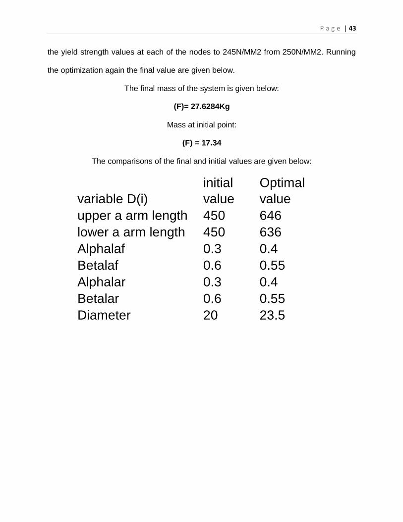
The comparisons of the final and initial values are given below:
variable D(i)
initial
value
Optimal
value
upper a arm length 450 646
lower a arm length 450 636
Alphalaf 0.3 0.4
Betalaf 0.6 0.55
Alphalar 0.3 0.4
Betalar 0.6 0.55
Diameter 20 23.5
P a g e | 44
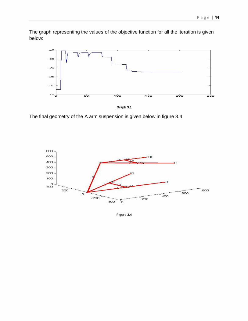
The graph representing the values of the objective function for all the iteration is given
below:
Graph 3.1
The final geometry of the A arm suspension is given below in figure 3.4
Figure 3.4
P a g e | 45
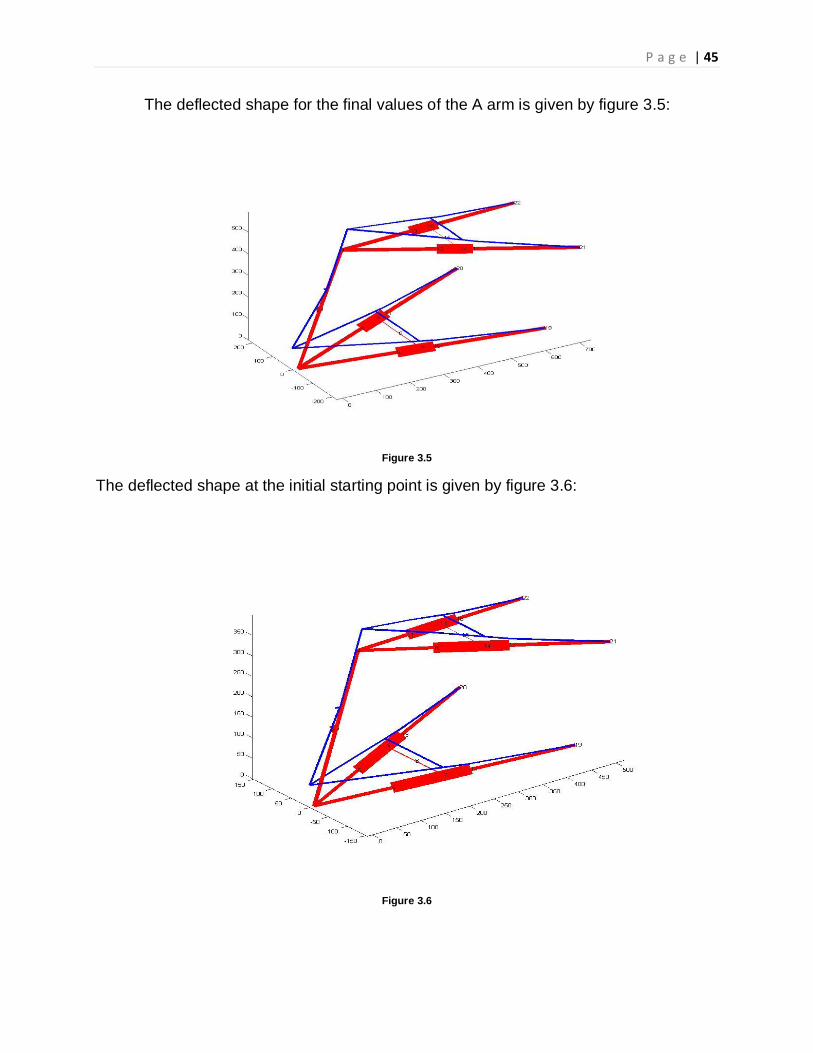
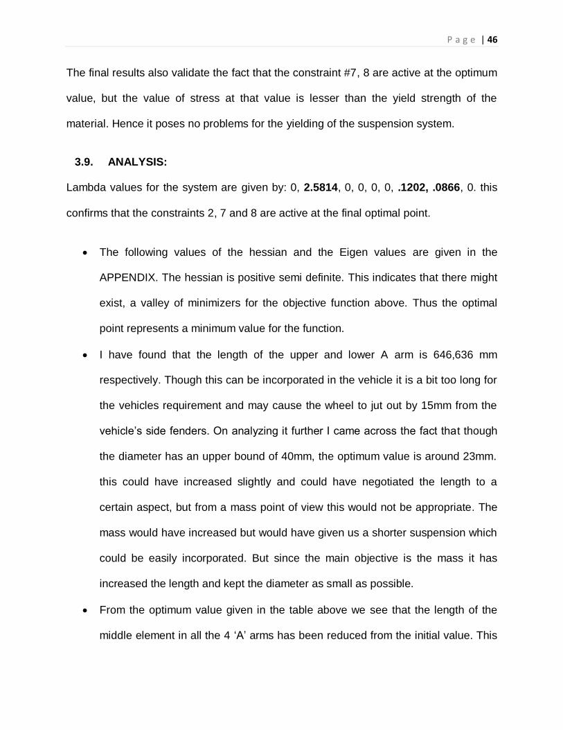
The deflected shape for the final values of the A arm is given by figure 3.5:
Figure 3.5
The deflected shape at the initial starting point is given by figure 3.6:
Figure 3.6
P a g e | 46
The final results also validate the fact that the constraint #7, 8 are active at the optimum
value, but the value of stress at that value is lesser than the yield strength of the
material. Hence it poses no problems for the yielding of the suspension system.
3.9. ANALYSIS:
Lambda values for the system are given by: 0, 2.5814, 0, 0, 0, 0, .1202, .0866, 0. this
confirms that the constraints 2, 7 and 8 are active at the final optimal point.
The following values of the hessian and the Eigen values are given in the
APPENDIX. The hessian is positive semi definite. This indicates that there might
exist, a valley of minimizers for the objective function above. Thus the optimal
point represents a minimum value for the function.
I have found that the length of the upper and lower A arm is 646,636 mm
respectively. Though this can be incorporated in the vehicle it is a bit too long for
the vehicles requirement and may cause the wheel to jut out by 15mm from the
vehicle‟s side fenders. On analyzing it further I came across the fact that though
the diameter has an upper bound of 40mm, the optimum value is around 23mm.
this could have increased slightly and could have negotiated the length to a
certain aspect, but from a mass point of view this would not be appropriate. The
mass would have increased but would have given us a shorter suspension which
could be easily incorporated. But since the main objective is the mass it has
increased the length and kept the diameter as small as possible.
From the optimum value given in the table above we see that the length of the
middle element in all the 4 „A‟ arms has been reduced from the initial value. This
P a g e | 47
must have happened cause the suspension arms need long flexible arms to
absorb the loads and the short rigid element in between just gives it a bit more
rigidity but doesn‟t help out with the load absorption purposes. This was in
expectation with the results I was expecting initially.
The final weight of the suspension system is 27.684Kg, which is quite heavier
when compared to the mass of the rigid suspension. Thus this increases the
unsprung mass, thereby slowing down the reaction of the suspension system.
At the final optimal solution three of the constraints are active as indicated by the
Lagrange multipliers. This indicates that the optimal doesn‟t lie at the interior
point of the function curve but at the boundary. This makes the problem highly
sensitive that is the solution is not a robust one since any error in the final value
of the variables could lead to the violation of the constraints. This could occur
due to manufacturing tolerances which could offset the optimal point by some
length and hence lead to constraint violation. Since the maximum jounce
constraint is active at the optimal point, this could lead to bottoming of the
suspension due to any defects either manufacturing or design of the part.
3.10. SUBSYSTEM TRADEOFFS:
The main objective function of my system was to reduce the mass of the
system, keeping in mind the stress levels at the nodes of the suspension. For a
compliant system the general mass was found to be higher than the regular
suspension system, which is not a good case when the dynamics of the
suspension is considered. For the compliant mechanism to be able to absorb
the loads and to keep the stress below required levels it needs longer arms and
P a g e | 48
thus the overall length of the system increases. For the dynamic analysis the
required length of the arms should be as minimum, as possible. This creates an
interesting tradeoff for the complete system optimization. In my case I have
considered the top plate connecting the upper a arms and holding the damper,
to be very small. In the damper placement analysis, this plate disappears
altogether and this will lead to a tradeoff in which the plate doesn‟t exist, and
the stress levels might vary. This also leads to an interesting tradeoff in the
sense that, the damper forces are going to act on the bottom plate which has
not been taken into consideration in my analysis. In my analysis I have
considered a fixed topology for the initial design, whereas in the kinematic
analysis the topology is going to be varied. This might create the maximum
stresses at different nodes, which may differ from the nodes taken into
consideration now. The final analysis will focus on evaluating the above
tradeoffs and finding out an optimal design to the solution.
P a g e | 49
4. DAMPER PLACEMENT ANALYSIS - by Karan Goyal
4.1 PROBLEM STATEMENT
The objective of this problem is to find the optimum position of the damper on the
suspension mechanism so as to minimize the displacement/travel in the vertical
direction. The position of the damper refers to the points where the damper is attached
to the mechanism. Minimum displacement/travel in the vertical direction is desired to
restrain violent impacts and to attenuate vibrations.
Compared to other vibration dampers, the fluid viscous damper is a favorable device as
its stiffness and damping coefficient are completely independent. The fluid viscous
damper generates damping by the liquid flowing through orifices or valves. Therefore,
the damping characteristics of the vehicle are analyzed by considering a mono-tube
passive hydraulic shock absorber attached between four links of the suspension
mechanism.
The response of a vehicle depends upon the vehicle suspension which in turn depends
upon the road input conditions. Road is the primary input for the vehicle suspension.
This road input could be nonlinear in nature due to the irregularities in the road surface.
Since the main objective is to find the optimum position of the damper and not design a
damper, a unit force was considered as an input for the vehicle suspension system.
A shock absorber in a car is designed to damp the oscillations of the suspension
springs in the car. Without this damping after a car passes over a bump, it will bounce
P a g e | 50
(oscillate) up and down many times rather than just once. Damping in shock absorbers
is obtained by forcing a piston to move through a liquid-filled cylinder with an
appropriate amount of fluid flow through or around the cylinder. This provides a drag
force that is approximately proportional to the speed with which the piston moves. Since
the damper shows a non linear behavior, it is difficult to construct a mathematical model
to find the optimal placement of the damper while taking into account the oil
characteristics, damper orifice dimensions and the size and length of the damper etc.
Therefore, to facilitate the process of analysis and design, the damping is approximately
taken to be linear. Also to include the effects of the size and length of the damper as
well as the oil characteristics and the effect of the orifice dimensions the damping
coefficient is considered to be one of the variables.
Also for the ease of calculations and to model the damper position as close to the real
conditions as possible, the upper end of the damper is considered to be fixed at a
random point on the chassis. The lower end of the damper is fixed to the mounting plate
that is connected to the two arms of the lower a-arm of the mechanism. The position of
this lower end of the damper is what we are really interested in, as after optimizing for
minimum displacement we will find a point where the damper would be connected to the
suspension mechanism. Thus we get three more variables. Two being the distance of
the two ends of the mounting plates from the fixed end of arms of the lower a-arm. The
other being the position of the point on the mounting plate where the damper is actually
connected. Doing this gives us the ability to position the damper anywhere on the plane
between the two arms of the lower a-arm.
P a g e | 51
4.2 NOMENCLATURE:
F: The external force applied
K : Stiffness of the suspension mechanism in N/mm
M : Mass of the vehicle in kg
C : Damping Coefficient
x1 : Position of the point on the lower link where the damper is attached
x2 : Position of the point on the lower link where the damper is attached
Y : Displacement/Travel in the vertical direction in mm
Ỳ : Velocity in mm/sec
Ÿ : Acceleration in mm/sec2
Laf: Length of the lower a-arm front in mm
Lar: Length of the lower a-arm rear in mm
Lambdat : the distance between the fixed end of the front link of the lower a-arm and the
point where the mounting plate is connected to the link in mm
Lambdab : the distance between the fixed end of the rear link of the lower a-arm and
the point where the mounting plate is connected to the link in mm
Lmp : length of the mounting plate in mm
P a g e | 52
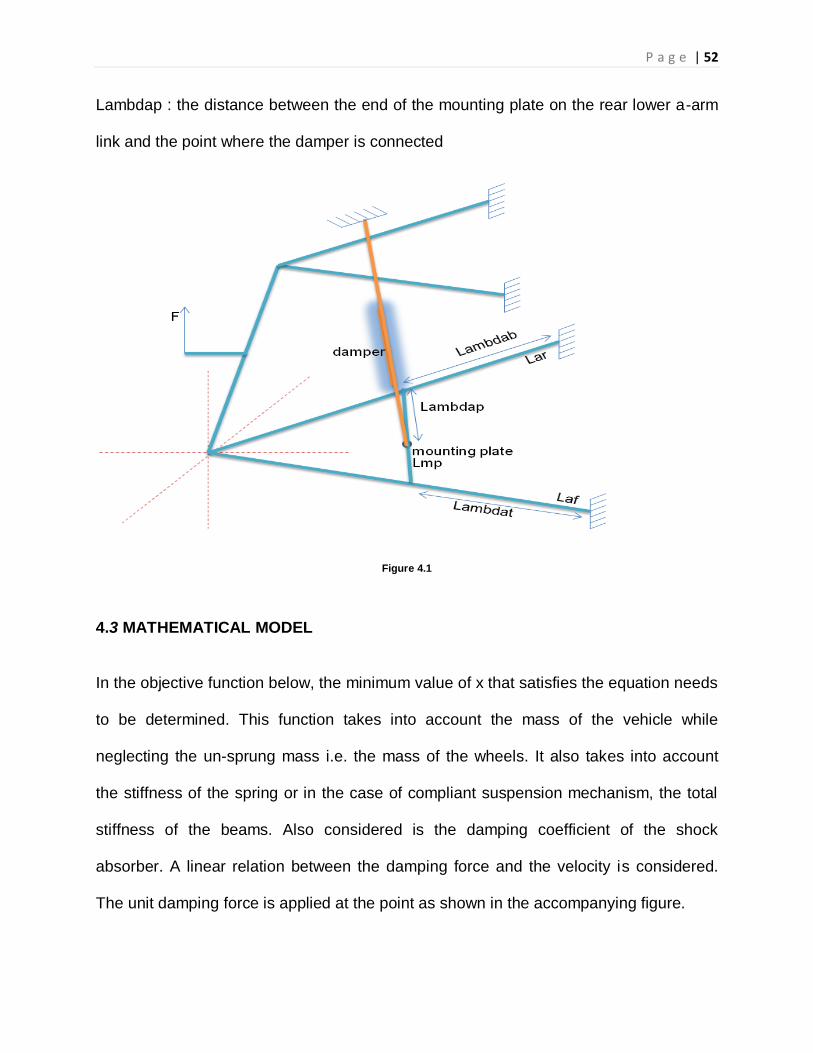
Lambdap : the distance between the end of the mounting plate on the rear lower a-arm
link and the point where the damper is connected
Figure 4.1
4.3 MATHEMATICAL MODEL
In the objective function below, the minimum value of x that satisfies the equation needs
to be determined. This function takes into account the mass of the vehicle while
neglecting the un-sprung mass i.e. the mass of the wheels. It also takes into account
the stiffness of the spring or in the case of compliant suspension mechanism, the total
stiffness of the beams. Also considered is the damping coefficient of the shock
absorber. A linear relation between the damping force and the velocity is considered.
The unit damping force is applied at the point as shown in the accompanying figure.
P a g e | 53
The lesser is the displacement of the piston in the damper, the lesser is the overall
displacement at the wheel. While we are minimizing the maximum displacement of the
damper, we will still be able to find the optimum position for the damper as a function of
the position of the damper‟s lower end on the mounting plate. The mathematical model
for this configuration is obtained using COMSOL and the optimization is performed
using MATLAB.
VARIABLES
Two of the variables are the position of the points on the beams of the lower a-arm
where the mounting plate is connected to the beams. The third variable is the position of
the lower end of the damper on the mounting plate itself. The fourth variable is the
damping coefficient. It was decided to include the damping coefficient itself to account
for the possibility of using a different damper with different working characteristics. The
design of the damper for minimum displacement could be a separate optimization
problem in itself.
CONSTRAINTS
The major constraints are on the position of the lower end of the damper on the
compliant mechanism. Its position could be anywhere in the plane between the two
beams of the lower a-arm. Thus it was decided to include a mounting plate that is
connected between the two beams of the lower a-arm. The damper can be mounted
anywhere on this plate. The constraints and hence the optimization problem would
determine the location of the point in this plane where the displacement would me
minimum. Other constraints were placed on the value of the damping coefficient. In the
P a g e | 54
absence of a mathematical model that would take into account the design
characteristics of a damper such as the oil properties, orifice diameter and size and the
diameter and the length of the damper, it was decided to limit the value of the damping
coefficient. Since only a unit force is being applied for the purpose of analysis, the
damping coefficient was reduced by a factor of hundred in the optimization model. Thus
the position of the damper is dictated by the length of the beams and the length of the
mounting plate. The position of the upper end of the damper is considered to be fixed to
the chassis to generate a model as close to the real solution.
PARAMETERS
For this subsystem the mass and the stiffness, the topology of the four bar mechanism
and the area of the cross section of the beams are the parameters. The fluid used while
finding the damping coefficient for the different dimensions of the damper is assumed to
be the same in all cases. Parametric study can be performed by using different set of
values for each of the parameters listed above. But for this optimization model, the
parametric study was performed only on the position of the fixed upped end of the
damper. The position of the fixed end of the damper on the chassis was changed in
case. This also led to a change in the length of the damper but its effect was assumed
to be included in the determination of the damping coefficient.
Note: This sub-system has a single degree of freedom as the only motion possible is in
the vertical direction.
P a g e | 55
4.4 SUMMARY MODEL
Objective Function is:
Min Y in f(Y) = MŸ + CỲ + KY – F
s.t.
g1: -C ≤ 0
g2: C -2 ≤ 0
g3: - Lambdap ≤0
g4: Lambdap - Lmp ≤0
g5: - Lambdat ≤0
g6: Lambdat - Laf ≤0
g7: - Lambdab ≤0
g8: Lambdab - Lar ≤0
4.5 MODEL ANALYSIS
The main optimization software being used for this subsystem was MATLAB. Initially the
position of the upper end of the damper was also considered to be a variable.
Constraints similar to the lower end of the damper were placed on the upper end too.
But it gave difficulty in determining the difference in the velocities of those two points for
determining the net displacement. Further, the use of two dampers instead of one was
also considered. This system would have one damper each connected to one of the
P a g e | 56
mounting plates. The other end of the dampers would be fixed. In this system too, using
MATLAB, it was difficult to obtain considerable displacement values.
Finally, it was decided to use a single damper with one end fixed to the chassis and the
other end connected to the compliant mechanism using a mounting plate. A quarter car
model was used for performing simulation. The mass was assumed to be constant and
the stiffness value of the compliant system was also assumed to be constant during the
parametric study. Only one variable i.e. is the damping coefficient is included in the
objective function. This variable is well bounded in both the directions. The damping
coefficient directly relates to the displacement if the damper and of the overall system.
The other variable relate directly to the position of the damper. Due to the absence of
any mathematical relation between the position of the damper and its displacement
characteristics, these variables could not be included in the objective function. But all
the constraints are active and none of the four variables is redundant. This was shown
during the parametric study. Varying the position of the fixed end of the damper gave
reasonably different values for the variables.
Using MATLAB, the optimized results for the four variables were obtained. These
values were obtained in a single iteration. After that the parametric study was
performed.
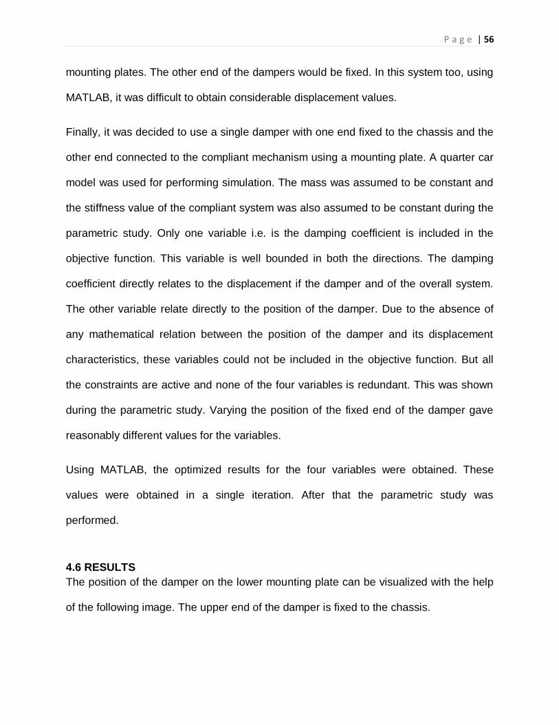
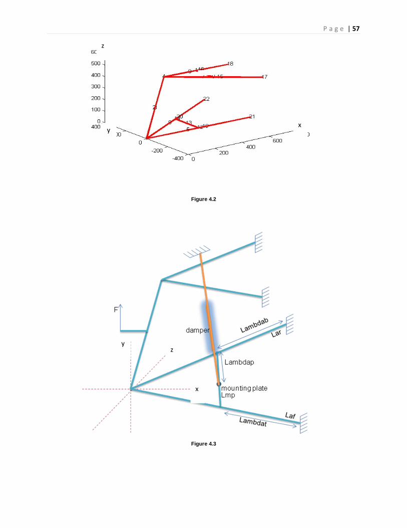
4.6 RESULTS
The position of the damper on the lower mounting plate can be visualized with the help
of the following image. The upper end of the damper is fixed to the chassis.
P a g e | 57
Figure 4.2
Figure 4.3
x
y z
z
y x
P a g e | 58
Sr.
No.
Parameter Design Variables Displacement
Fixed Point Lambdat Lambdab Lambdap C
1 [400 0 300] 0.3 0.3 0.9 2 9.7663e-004
2 [350 0 300] 0.7956 0.8 0.3992 .9991 9.7673e-004
3 [200 0 300] 0.3 0.3 0.8977 1.9998 9.5804e-004
4 [400 0 200] .7903 .8 .4065 .9938 9.7600e-004
5 [400 0 100] .3 .3 .8977 1.9998 9.5354e-004
6 [400 300 300] .3 .3 .9 2 9.9714e-004
7 [400 200 300] .3 .3 .9 2 9.8415e-004
8 [400 100 300] .7919 .8 .4042 .9954 9.7762e-004
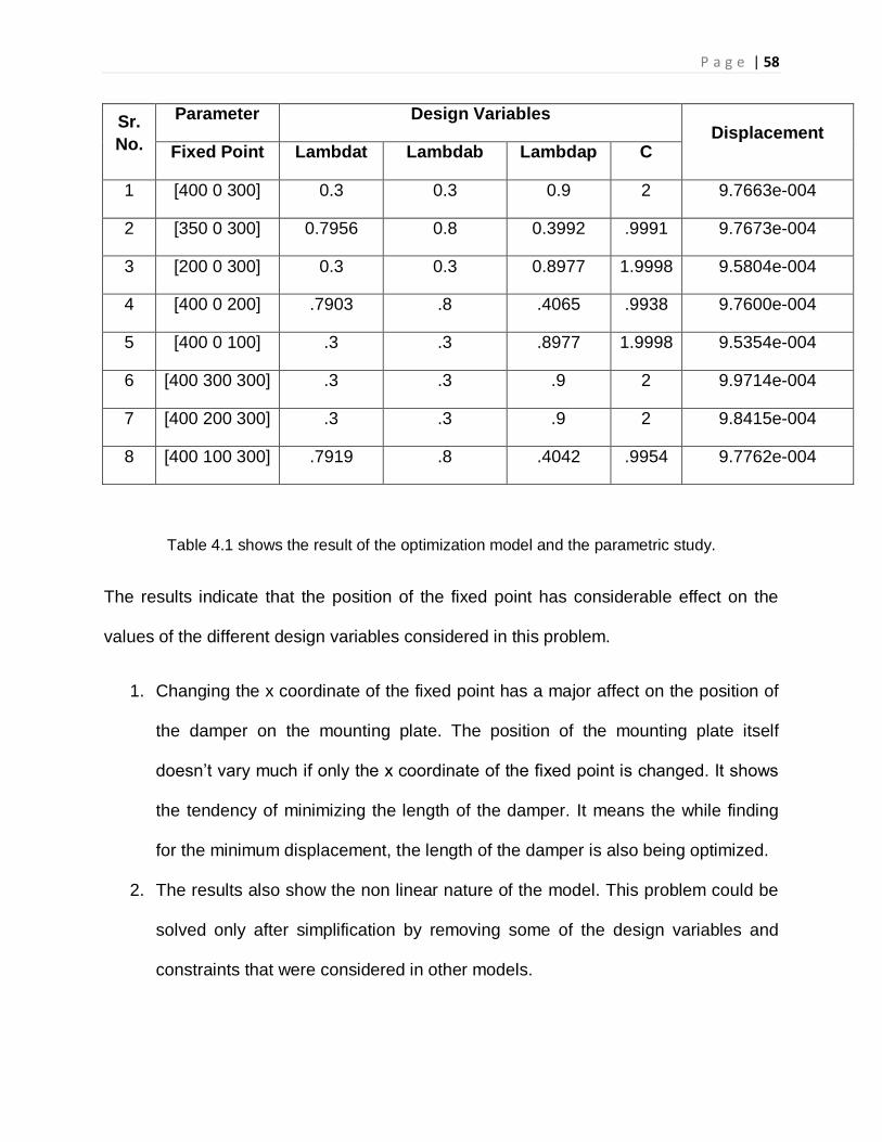
Table 4.1 shows the result of the optimization model and the parametric study.
The results indicate that the position of the fixed point has considerable effect on the
values of the different design variables considered in this problem.
1. Changing the x coordinate of the fixed point has a major affect on the position of
the damper on the mounting plate. The position of the mounting plate itself
doesn‟t vary much if only the x coordinate of the fixed point is changed. It shows
the tendency of minimizing the length of the damper. It means the while finding
for the minimum displacement, the length of the damper is also being optimized.
2. The results also show the non linear nature of the model. This problem could be
solved only after simplification by removing some of the design variables and
constraints that were considered in other models.
P a g e | 59
3. The parametric study also shows that, the position of the fixed point would have
a big impact on the overall displacement. It is shown by the fact that for the
different positions of the fixed point, we get same values for the variables but
different value for the overall displacement.
4. The nature of results obtained in the parametric study also highlight that the
length of the damper may also be an important factor in the determining the
placement of the damper. If we take the length of the damper into consideration,
we would also need to consider other design variables of the damper such as the
diameter, oil viscosity, orifice diameter etc. Thus, a more complex model would
be required.
5. While considering the length of the damper, we need to be extra careful with
setting the constraints/bounds on the length of the damper. As shown in the
results, decreasing the length may lead to a lower displacement, but an
extremely small damper may not be feasible. One way of overcoming this could
be the alignment of the damper at certain angles to get the same damping
characteristics.
6. From the parametric study we have been able to establish that the placement of
the damper in an automotive suspension system has considerable effect on the
displacement characteristics of the damper.
P a g e | 60
4.7 CONCLUSION & FUTURE WORK
The future work may involve creation of more complex mathematical models for taking
into consideration different damper characteristics. Taking just both the ends of the
damper as free and not fixed would involve an exhaustive study into the relationship
between the velocity difference of the two free points and the damping force. Design of
the damper could be considered a separate sub-system in itself.
P a g e | 61
FINAL SYSTEM INTEGRATION
For the final system integration we considered various different objectives like the best
kinematic topology, the best natural frequency and the best mass for the compliant A-
arm suspension. On analyzing the different objectives we came to the conclusion that
the main requirement for the suspension would be to reduce the mass of the compliant
A-arm suspension. The mass plays a very important role in the performance of a
suspension and can make a lot of difference. Thus minimizing the mass seemed to
increase the performance by a bigger margin when compared to the other objectives.
Thus minimizing the mass became our final objective function which was subjected to
various constraints derived from other subsystems.
Final Objective: MIN: F = MASS
5.2. CONSTRAINTS:
Since we carried over the structural optimization objective to our final system objective
the constraints that were placed in the structural optimization were all valid constraints
for the final system integration. Those are given by:
G1 =w1-jmax<=0
G2 =jmin-w1<=0
G3 =(x4+x1)-cambmin<=0
G4 =thz3-stirmin<=0
G5 =uy2-longdpmax<=0
G6 =abs (Z18) +abs (Y18)-yield1<=0
G7 =abs (Z17) +abs (Y17)-yield1<=0
P a g e | 62
G8 =abs (Z22) +abs (Y22)-yield1<=0
G9 =abs (Z21) +abs (Y21)-yield1<=0 The additional constraints that were added form the different subsystem optimization are given as follows.
G10 =1-nat
G11 = riset-0.8
G12 = 0.1-riset
The constraint g10 places a lower bound on the natural frequency derived from
Mukunds dynamic optimization. The lower bound is given as 1Hz. This is selected
because 1Hz is the maximum natural frequency for a general automobile, Hence the
value.
The constraints g11 and g12 basically place a lower and upper bound on the rise time
of the damper. This is generally taken as an ideal rise time for the vehicle of our class.
Hence it is bound from the top and from the bottom. A very short rise time would disrupt
passenger comfort and a very large rise time will allow the suspension to vibrate for a
longer time. This range basically provides an ideal range for the rise time to be in.
The next sets of constraints are derived from Girish‟s kinematic optimization. It places a
constraint on the maximum angle of rotation for the suspension arms and on the
kinematic jounce of the suspension.
G13 = 0.19-kinob (Gvar)
G14= gcons (7)
G15 = gcons (8)
G16=gcons (9)
G17=gcons (10)
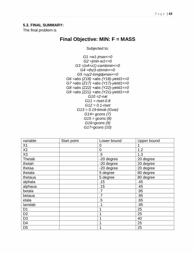
P a g e | 63
5.3. FINAL SUMMARY:
The final problem is
Final Objective: MIN: F = MASS
Subjected to:
G1 =w1-jmax<=0 G2 =jmin-w1<=0
G3 =(x4+x1)-cambmin<=0 G4 =thz3-stirmin<=0
G5 =uy2-longdpmax<=0 G6 =abs (Z18) +abs (Y18)-yield1<=0 G7 =abs (Z17) +abs (Y17)-yield1<=0 G8 =abs (Z22) +abs (Y22)-yield1<=0 G9 =abs (Z21) +abs (Y21)-yield1<=0
G10 =2-nat G11 = riset-0.8 G12 = 0.1-riset
G13 = 0.19-kinob (Gvar) G14= gcons (7) G15 = gcons (8) G16=gcons (9)
G17=gcons (10)
variable Start point Lower bound Upper bound
X1 0 1
X2 0 1.2
X3 .5 1.3
Thetab -20 degree 20 degree
thetah -20 degree 20 degree
thetaa -20 degree 20 degree
thetala 5 degree 80 degree
thetaua 5 degree 80 degree
alphala .15 .45
alphaua .15 .45
betala .7 .95
betaua .7 .95
etala .5 .65
lamdab .1 .95
D1 1 25
D2 1 25
D3 1 40
D4 1 25
D5 1 25
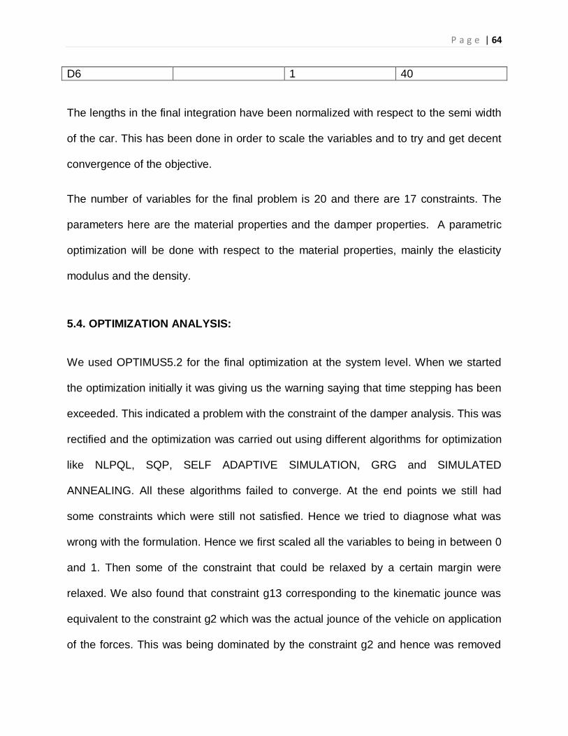
P a g e | 64
D6 1 40
The lengths in the final integration have been normalized with respect to the semi width
of the car. This has been done in order to scale the variables and to try and get decent
convergence of the objective.
The number of variables for the final problem is 20 and there are 17 constraints. The
parameters here are the material properties and the damper properties. A parametric
optimization will be done with respect to the material properties, mainly the elasticity
modulus and the density.
5.4. OPTIMIZATION ANALYSIS:
We used OPTIMUS5.2 for the final optimization at the system level. When we started
the optimization initially it was giving us the warning saying that time stepping has been
exceeded. This indicated a problem with the constraint of the damper analysis. This was
rectified and the optimization was carried out using different algorithms for optimization
like NLPQL, SQP, SELF ADAPTIVE SIMULATION, GRG and SIMULATED
ANNEALING. All these algorithms failed to converge. At the end points we still had
some constraints which were still not satisfied. Hence we tried to diagnose what was
wrong with the formulation. Hence we first scaled all the variables to being in between 0
and 1. Then some of the constraint that could be relaxed by a certain margin were
relaxed. We also found that constraint g13 corresponding to the kinematic jounce was
equivalent to the constraint g2 which was the actual jounce of the vehicle on application
of the forces. This was being dominated by the constraint g2 and hence was removed
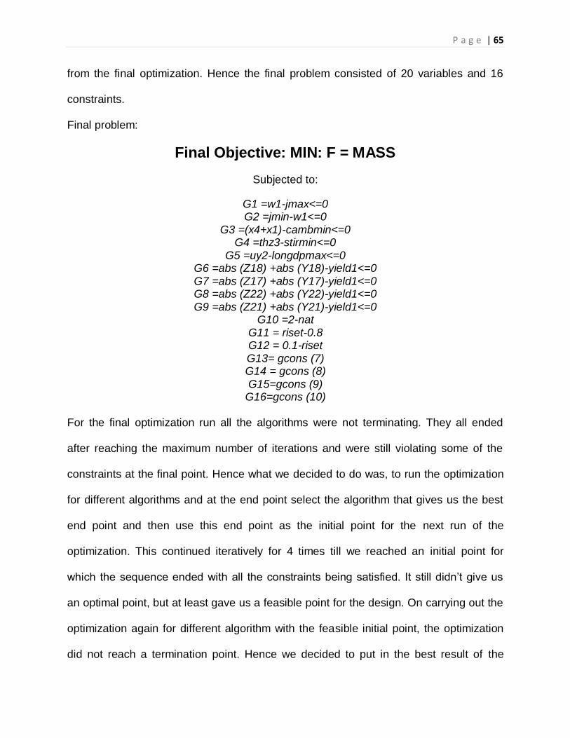
P a g e | 65
from the final optimization. Hence the final problem consisted of 20 variables and 16
constraints.
Final problem:
Final Objective: MIN: F = MASS
Subjected to:
G1 =w1-jmax<=0 G2 =jmin-w1<=0
G3 =(x4+x1)-cambmin<=0 G4 =thz3-stirmin<=0
G5 =uy2-longdpmax<=0 G6 =abs (Z18) +abs (Y18)-yield1<=0 G7 =abs (Z17) +abs (Y17)-yield1<=0 G8 =abs (Z22) +abs (Y22)-yield1<=0 G9 =abs (Z21) +abs (Y21)-yield1<=0
G10 =2-nat G11 = riset-0.8 G12 = 0.1-riset G13= gcons (7) G14 = gcons (8) G15=gcons (9)
G16=gcons (10)
For the final optimization run all the algorithms were not terminating. They all ended
after reaching the maximum number of iterations and were still violating some of the
constraints at the final point. Hence what we decided to do was, to run the optimization
for different algorithms and at the end point select the algorithm that gives us the best
end point and then use this end point as the initial point for the next run of the
optimization. This continued iteratively for 4 times till we reached an initial point for
which the sequence ended with all the constraints being satisfied. It still didn‟t give us
an optimal point, but at least gave us a feasible point for the design. On carrying out the
optimization again for different algorithm with the feasible initial point, the optimization
did not reach a termination point. Hence we decided to put in the best result of the
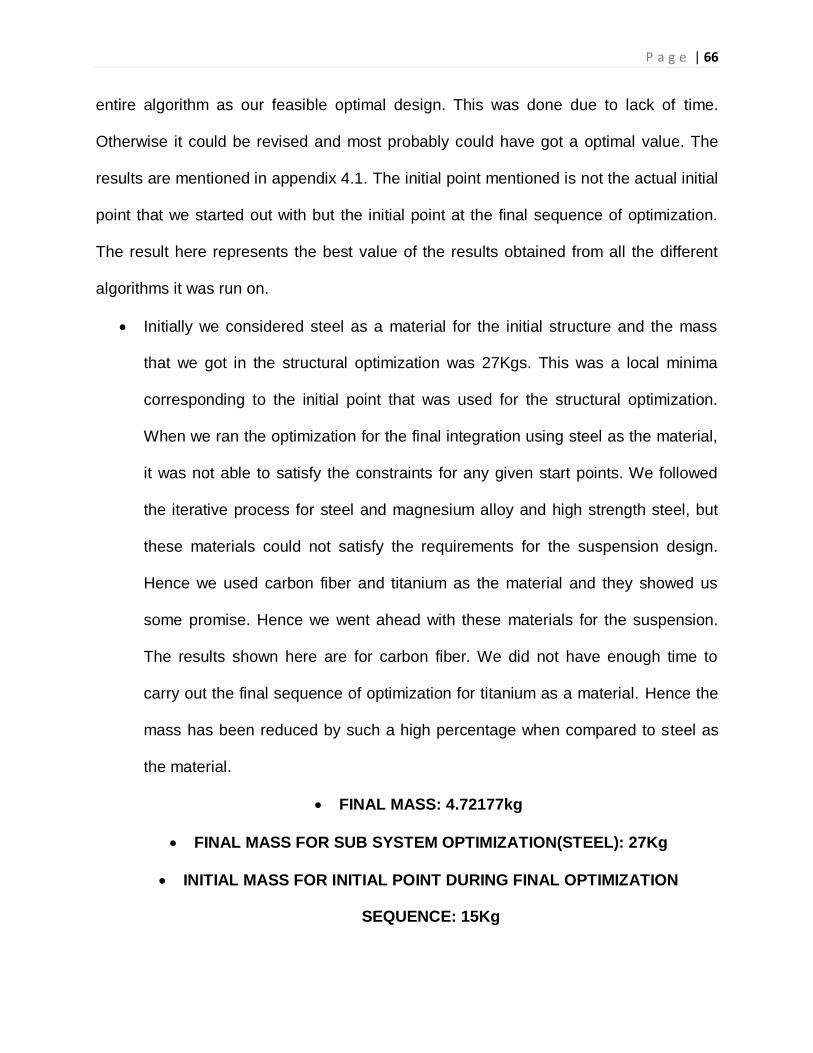
P a g e | 66
entire algorithm as our feasible optimal design. This was done due to lack of time.
Otherwise it could be revised and most probably could have got a optimal value. The
results are mentioned in appendix 4.1. The initial point mentioned is not the actual initial
point that we started out with but the initial point at the final sequence of optimization.
The result here represents the best value of the results obtained from all the different
algorithms it was run on.
Initially we considered steel as a material for the initial structure and the mass
that we got in the structural optimization was 27Kgs. This was a local minima
corresponding to the initial point that was used for the structural optimization.
When we ran the optimization for the final integration using steel as the material,
it was not able to satisfy the constraints for any given start points. We followed
the iterative process for steel and magnesium alloy and high strength steel, but
these materials could not satisfy the requirements for the suspension design.
Hence we used carbon fiber and titanium as the material and they showed us
some promise. Hence we went ahead with these materials for the suspension.
The results shown here are for carbon fiber. We did not have enough time to
carry out the final sequence of optimization for titanium as a material. Hence the
mass has been reduced by such a high percentage when compared to steel as
the material.
FINAL MASS: 4.72177kg
FINAL MASS FOR SUB SYSTEM OPTIMIZATION(STEEL): 27Kg
INITIAL MASS FOR INITIAL POINT DURING FINAL OPTIMIZATION
SEQUENCE: 15Kg
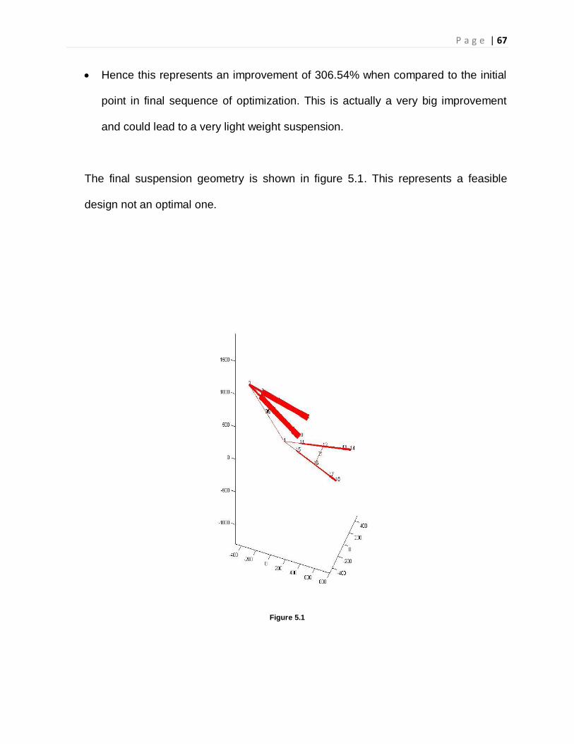
P a g e | 67
Hence this represents an improvement of 306.54% when compared to the initial
point in final sequence of optimization. This is actually a very big improvement
and could lead to a very light weight suspension.
The final suspension geometry is shown in figure 5.1. This represents a feasible
design not an optimal one.
Figure 5.1
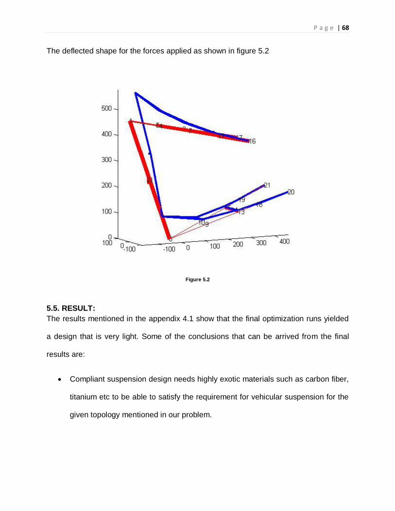
P a g e | 68
The deflected shape for the forces applied as shown in figure 5.2
Figure 5.2
5.5. RESULT:
The results mentioned in the appendix 4.1 show that the final optimization runs yielded
a design that is very light. Some of the conclusions that can be arrived from the final
results are:
Compliant suspension design needs highly exotic materials such as carbon fiber,
titanium etc to be able to satisfy the requirement for vehicular suspension for the
given topology mentioned in our problem.
P a g e | 69
Compliant suspension need long link lengths to be able to satisfy the stress
requirements. This was in expectation with what we thought would be the final
results.
The given design requires a very large thetaua to be able to satisfy the
requirements of the suspension. This is not a general design. Most A arm
suspension have a comparatively smaller thetaua when compared to the design
of the compliant suspension.
In our optimization runs we found that sequential quadratic programming (SQP)
kept giving us the best results among all the other algorithms. Even the final best
feasible result is from the run made in SQP.
The final mass is very low for an A arm suspension and if implemented could
improve the ride and handling characteristic of a vehicle as it reduces the
unsprung mass of the vehicle by a large margin. General rigid A arm suspension
made of steel weigh in around 12-15 kilos. We have not been able to find results
on how much would a rigid A-arm suspension made of carbon fiber would weigh
but we estimate that it would be higher than the corresponding compliant
suspension.
5.6. FUTURE WORK:
1. Topology optimizations to be done to determine an optimal topology design for a
complaint A arm suspension.
2. Different materials to be considered when carrying out the optimization process.
P a g e | 70
3. Multiple damper placements can be considered for even better damping results.
MUCHAS GRACIAS (THANKS)
We would like to thank Jarod Kelly for his help and support to us during our
optimization analysis. This would not have been possible without his useful
insights into our projects.
We would like to thank Dr. Michael Kokkolaras for making this a very interesting
Course and giving us a very useful insight about the basics of optimization.
We would also like to thank James Allison for helping us out during the initial
stages of our optimization with the subsystem division.
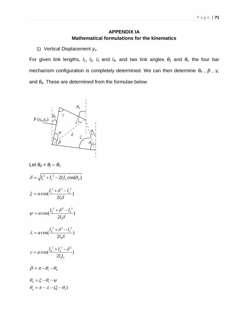
P a g e | 71
APPENDIX IA
Mathematical formulations for the kinematics
1) Vertical Displacement yv.
For given link lengths, l1, l2, l3 and l4, and two link angles θ1 and θt, the four bar
mechanism configuration is completely determined. We can then determine θh , β , γ,
and θa. These are determined from the formulae below
Let θd = θt – θ1
2 2
1 2 1 22 cos( )dl l l l
2 2 2
1 2
1
cos( )2
l la
l
2 2 2
3 4
3
cos( )2
l la
l
2 2 2
4 3
4
cos( )2
l la
l
2 2 2
4 3
4 3
cos( )2
l la
l l
t h
1
1( )
h
a
θh
θa
θt β
γ
λ
ψ θ1 δ
ξ
P (xp,yp)
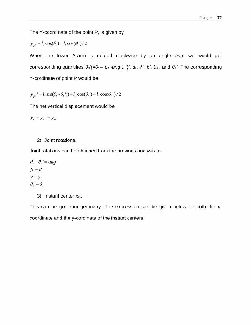
P a g e | 72
The Y-coordinate of the point P, is given by
1 2 3cos( ) cos( ) / 2p t hy l l
When the lower A-arm is rotated clockwise by an angle ang, we would get
corresponding quantities θd’(=θt – θ1 -ang ), ξ’, ψ’, λ’, β’, θh’, and θa’. The corresponding
Y-cordinate of point P would be
1 2 3' sin( - ')) cos( ') cos( ') / 2p c t t t hy l l l
The net vertical displacement would be
1 1'v p py y y
2) Joint rotations.
Joint rotations can be obtained from the previous analysis as
'
'
'
'
t t
a a
ang
3) Instant center xin.
This can be got from geometry. The expression can be given below for both the x-
coordinate and the y-cordinate of the instant centers.
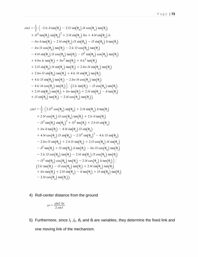
P a g e | 73
4) Roll-center distance from the ground
5) Furthermore, since l1 ,l2, θ1 and θt are variables, they determine the fixed link and
one moving link of the mechanism.
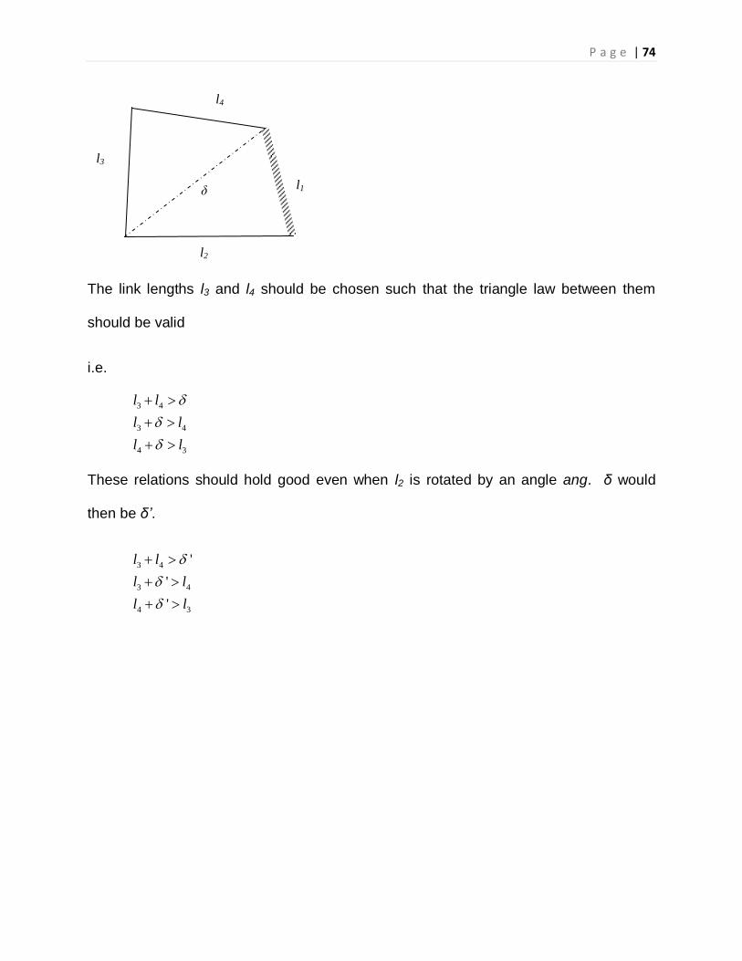
P a g e | 74
The link lengths l3 and l4 should be chosen such that the triangle law between them
should be valid
i.e.
3 4
3 4
4 3
l l
l l
l l
These relations should hold good even when l2 is rotated by an angle ang. δ would
then be δ’.
3 4
3 4
4 3
'
'
'
l l
l l
l l
l2
l1
l4
l3
δ
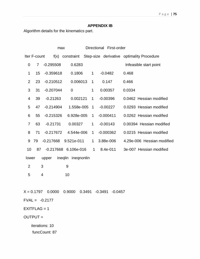
P a g e | 75
APPENDIX IB
Algorithm details for the kinematics part.
max Directional First-order
Iter F-count f(x) constraint Step-size derivative optimality Procedure
0 7 -0.295508 0.6283 Infeasible start point
1 15 -0.359618 0.1806 1 -0.0482 0.468
2 23 -0.210512 0.006013 1 0.147 0.466
3 31 -0.207044 0 1 0.00357 0.0334
4 39 -0.21263 0.002121 1 -0.00396 0.0462 Hessian modified
5 47 -0.214904 1.558e-005 1 -0.00227 0.0293 Hessian modified
6 55 -0.215326 6.928e-005 1 -0.000411 0.0262 Hessian modified
7 63 -0.21731 0.00327 1 -0.00143 0.00394 Hessian modified
8 71 -0.217672 4.544e-006 1 -0.000362 0.0215 Hessian modified
9 79 -0.217668 9.521e-011 1 3.88e-006 4.29e-006 Hessian modified
10 87 -0.217668 6.106e-016 1 8.4e-011 3e-007 Hessian modified
lower upper ineqlin ineqnonlin
2 3 9
5 4 10
X = 0.1797 0.0000 0.9000 0.3491 -0.3491 -0.0457
FVAL = -0.2177
EXITFLAG = 1
OUTPUT =
iterations: 10
funcCount: 87
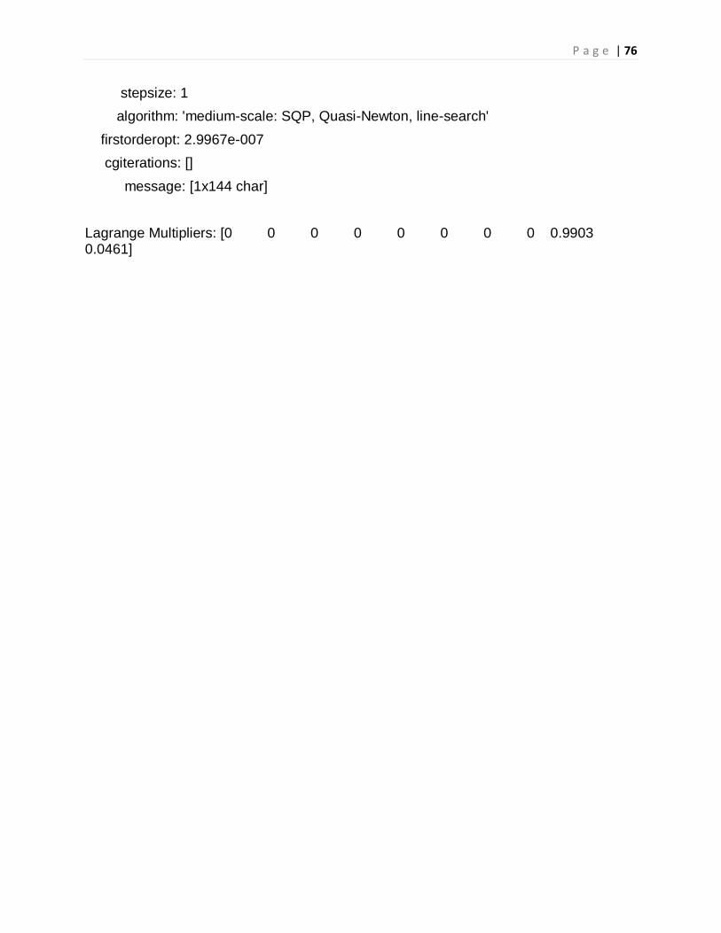
P a g e | 76
stepsize: 1
algorithm: 'medium-scale: SQP, Quasi-Newton, line-search'
firstorderopt: 2.9967e-007
cgiterations: []
message: [1x144 char]
Lagrange Multipliers: [0 0 0 0 0 0 0 0 0.9903 0.0461]
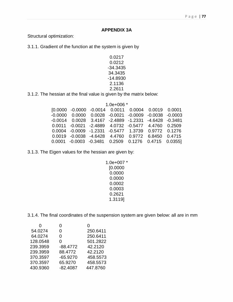
P a g e | 77
APPENDIX 3A
Structural optimization:
3.1.1. Gradient of the function at the system is given by
0.0217 0.0212
-34.3435 34.3435 -14.8930 2.1136 2.2611
3.1.2. The hessian at the final value is given by the matrix below:
1.0e+006 * [0.0000 -0.0000 -0.0014 0.0011 0.0004 0.0019 0.0001 -0.0000 0.0000 0.0028 -0.0021 -0.0009 -0.0038 -0.0003 -0.0014 0.0028 3.4167 -2.4889 -1.2331 -4.6428 -0.3481 0.0011 -0.0021 -2.4889 4.0732 -0.5477 4.4760 0.2509 0.0004 -0.0009 -1.2331 -0.5477 1.3739 0.9772 0.1276 0.0019 -0.0038 -4.6428 4.4760 0.9772 6.8450 0.4715 0.0001 -0.0003 -0.3481 0.2509 0.1276 0.4715 0.0355]
3.1.3. The Eigen values for the hessian are given by:
1.0e+007 * [0.0000 0.0000 0.0000 0.0002 0.0003 0.2621 1.3119]
3.1.4. The final coordinates of the suspension system are given below: all are in mm
0 0 0 54.0274 0 250.6411 64.0274 0 250.6411 128.0548 0 501.2822 239.3959 -88.4772 42.2120 239.3959 88.4772 42.2120 370.3597 -65.9270 458.5573 370.3597 65.9270 458.5573 430.9360 -82.4087 447.8760
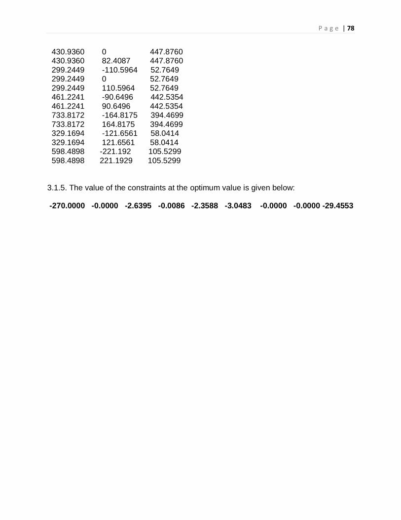
P a g e | 78
430.9360 0 447.8760 430.9360 82.4087 447.8760 299.2449 -110.5964 52.7649 299.2449 0 52.7649 299.2449 110.5964 52.7649 461.2241 -90.6496 442.5354 461.2241 90.6496 442.5354 733.8172 -164.8175 394.4699 733.8172 164.8175 394.4699 329.1694 -121.6561 58.0414 329.1694 121.6561 58.0414 598.4898 -221.192 105.5299 598.4898 221.1929 105.5299
3.1.5. The value of the constraints at the optimum value is given below:
-270.0000 -0.0000 -2.6395 -0.0086 -2.3588 -3.0483 -0.0000 -0.0000 -29.4553
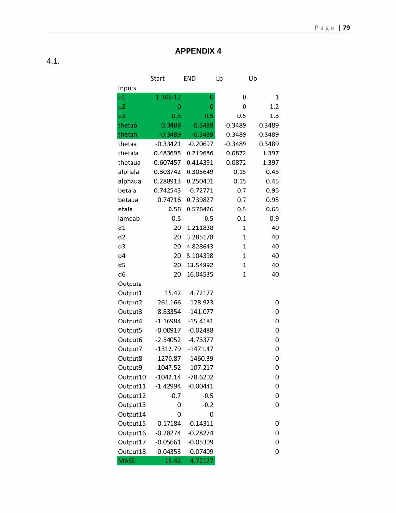
P a g e | 79
APPENDIX 4
4.1.
Start END Lb Ub
Inputs
u1 1.30E-12 0 0 1
u2 0 0 0 1.2
u3 0.5 0.5 0.5 1.3
thetab 0.3489 0.3489 -0.3489 0.3489
thetah -0.3489 -0.3489 -0.3489 0.3489
thetaa -0.33421 -0.20697 -0.3489 0.3489
thetala 0.483695 0.219686 0.0872 1.397
thetaua 0.607457 0.414391 0.0872 1.397
alphala 0.303742 0.305649 0.15 0.45
alphaua 0.288913 0.250401 0.15 0.45
betala 0.742543 0.72771 0.7 0.95
betaua 0.74716 0.739827 0.7 0.95
etala 0.58 0.578426 0.5 0.65
lamdab 0.5 0.5 0.1 0.9
d1 20 1.211838 1 40
d2 20 3.285178 1 40
d3 20 4.828643 1 40
d4 20 5.104398 1 40
d5 20 13.54892 1 40
d6 20 16.04535 1 40
Outputs
Output1 15.42 4.72177
Output2 -261.166 -128.923 0
Output3 -8.83354 -141.077 0
Output4 -1.16984 -15.4181 0
Output5 -0.00917 -0.02488 0
Output6 -2.54052 -4.73377 0
Output7 -1312.79 -1471.47 0
Output8 -1270.87 -1460.39 0
Output9 -1047.52 -107.217 0
Output10 -1042.14 -78.6202 0
Output11 -1.42994 -0.00441 0
Output12 -0.7 -0.5 0
Output13 0 -0.2 0
Output14 0 0
Output15 -0.17184 -0.14311 0
Output16 -0.28274 -0.28274 0
Output17 -0.05661 -0.05309 0
Output18 -0.04353 -0.07409 0
MASS 15.42 4.72177
P a g e | 80
REFERENCES:
1) Allred, T., Howell, L. L., Magleby, S. P., Todd, R. H., “ The Compliant A-Arm
suspension”, Proceedings of IMECE‟ 03, Wahington, D. C., November 15-21,
2003
2) Principles of optimal design. Modeling and computation. Panos.y.Papalambros
and Douglass.J.Wilde
3) “One-piece compliant Automotive suspension mechanism”, an ME 450 report
chaired by Prof. Sridhar Kota, April 22, 1994.
4) Gillespie, Thomas D., Fundamentals of Vehicle Dynamics, SAE, 1992.
5) Howell, Midha and Norton, Evaluation of Equivalent Spring Stiffness for use in a
Pseudo Rigid Body model of Large Deflection Compliant Mechanisms, 1996,
ASME Journal of Mechanisms Design / Vol. 118
6) Kota, Kikuchi and Joo, Topological synthesis of Compliant Mechanisms Using
Linear Beam Elements, 2000, Mech. Struc. & Mach., 28(4)
7) Bastow, Howard, Whitehead, Car suspension And Handling, SAE, Warrandale,
PA
8) http://www.fourwheeler.com/techarticles/suspension/129_0601_2005_gmc_duram
ax_jounce_shocks/photo_02.html
9) COMPLIANT MECHANISMS BY LARRY HOWELL
10) Halliday, resnick, and Walter, 5th edition, chapter 16, special attention to section
16-8 (damped simple harmonic motion)
P a g e | 81
11) Mechanical characteristics of oil-damping shock absorber for protection of
electronic-packaging components by yang ping, Research Center of Micro-Nano
Science and Technology, Jiangsu University, Zhenjiang, China
12) Development and experimental verification of a parametric model of an
automotive damper, a thesis by Kirk Shawn Rhoades, Texas A&M University
13) Dixon, J. C. “Shock Absorber Handbook”, SAE International, Feb. 1999

P a g e | 82
Recommended