Computational and Modeling Strategies for Cell
Motility
Qi Wang and Xiaofeng Yang∗, David Adalsteinsson†,
Timothy C. Elston‡, Ken Jacobson§, and Maryna Kapustina¶, and M. Gregory Forest∥
Abstract
We review emerging strategies and progress toward modeling and simulation of 3Dcell morphology and dynamics of a motile cell. We then describe our approach, basedon phase field modeling, that is flexible enough to incorporate distinct substructureswithin a cell, how they physically interact, mobile and reacting chemical species, andchemical-mechanical transduction. We posit a modeling foundation which addressesthe collective dynamics and morphology of a cell in response to physical forcing orboundary conditions at the cell membrane as well as internal signaling pathways. Ourmodeling approach is conditioned on the requirement that we can numerically simulatethe model equations consistent with laboratory experiments and compare model resultswith laboratory data of whole cell morphology and dynamics or more specific featuressuch as localized contractile waves. The proposed whole cell model is an integrationof sub-models: for cell membrane dynamics, external boundary conditions (with othercells, external buffer, solid substrates), multiple substructures with highly contrastingproperties (membrane, cortical layer, cytosol, nucleus), complex viscoelastic constitutivelaws and evolving free surface domains for each substructure, biochemical reaction anddiffusion of key protein species, and activation (localized forcing) through chemical-mechanical transduction. We summarize the literature on substructure modeling andactivation mechanisms, and then present an integrated modeling framework. The aim isto model diverse modes of motile cells; our first target is a model explanation of sustainedcell oscillations [69, 40, 92, 22, 91]. In order for the model to have predictive value, thecell model has to exhibit sufficient conditions for cell oscillations, while illustratingmechanisms which would lead to cessation of oscillations and transition to a differentdynamic modality. To simulate the model, we have to strike a compromise betweenbiological detail and computational feasibility. The modeling framework is a phase field(or diffuse interface) methodology which has already yielded progress in cell modelingand which provides a platform for future development. The success of the phase fieldapproach rests on the ability to formulate sufficiently accurate energy functionals foreach of the substructures, their interaction at interfaces, and spatio-temporal chemicalactivation within evolving substructures. Our contention is that sufficient progress has
∗Department of Mathematics and NanoCenter, University of South Carolina, Columbia, SC 29208†Department of Mathematics, University of North Carolina at Chapel Hill, Chapel Hill, NC 27599‡Department of Pharmacology, University of North Carolina at Chapel Hill, Chapel Hill, NC 27599§Department of Cell and Developmental Biology and Lineberger Comprehensive Cancer Center, Univer-
sity of North Carolina at Chapel Hill, Chapel Hill, NC 27599¶Department of Cell and Developmental Biology, University of North Carolina at Chapel Hill, Chapel
Hill, NC 27599∥Department of Mathematics and Institute for Advanced Materials, University of North Carolina at
Chapel Hill, Chapel Hill, NC 27599
1
been made on the energetics, detection and tracking of signaling proteins, and materialcharacterization of cell biology (cf. [83] and the entire issue of the New Journal ofPhysics, Volume 9, 2007) that an approach of this nature is feasible.
1 Introduction
A predictive simulation of the dynamics of a living cell remains a fundamental modeling
and computational challenge. The challenge does not even make sense unless one specifies
the level of detail and the phenomena of interest, whether the focus is on near-equilibrium
or strongly non-equilibrium behavior, and on localized, subcellular, or global cell behavior.
Therefore, choices have to be made clear at the outset, ranging from distinguishing between
prokaryotic and eukaryotic cells, specificity within each of these types, whether the cell is
“normal”, whether one wants to model mitosis, blebs, migration, division, deformation due
to confined flow as with red blood cells, and the level of microscopic detail for any of these
processes. The review article by Hoffman and Crocker [52] is both an excellent overview of
cell mechanics and an inspiration for our approach. One might be interested, for example,
in duplicating the intricate experimental details reported in [47]: “actin polymerization
periodically builds a mechanical link, the lamellipodium, connecting myosin motors with
the initiation of adhesion sites, suggesting that the major functions driving motility are
coordinated by a biomechanical process”, or to duplicate experimental evidence of traveling
waves in cells recovering from actin depolymerization [46, 40]. Modeling studies of lamel-
lipodial structure, protrusion and retraction behavior range from early mechanistic models
[89], to more recent deterministic [118, 103] and stochastic [55] approaches with significant
biochemical and structural detail. Recent microscopic-macroscopic models and algorithms
for cell blebbing have been developed by Young and Mitran [120], which update cytoskeletal
microstructure via statistical sampling techniques together with fluid variables. Alterna-
tively, whole cell compartment models (without spatial details) of oscillations in spreading
cells have been proposed [40, 96, 115] which show positive and negative feedback mecha-
nisms between kinetics and mechanics, and which are sufficient to describe a modality of
sustained cell oscillations. The generalization of such a nonlinear limit cycle mechanism
to include 3D spatial sub-structures consistent with cell mechanics, and biochemical kinet-
ics and diffusion, charts a path that our group has elected. Detailed microscopic features
are resolved through effective or collective properties of each substructure, which are dy-
namically updated by chemical species and processes. This choice is guided by a series of
developments in the biophysics community on cell structure and rheology (cf. New Journal
of Physics, Volume 9, 2007), together with recent progress on the biochemical feedback
mechanisms associated with cell morphological oscillations [69, 40] as well as other dynamic
cell modes.
Our approach is likewise guided by multiphase (implying differentiated substructures)
modeling and computational tools developed for analogous applications such as biofilms
[124, 125, 112, 74] and complex fluid mixtures (polymer dispersed nematic rods [73, 42],
liquid crystal drops in viscous fluids [43, 123]). We integrate these approaches to propose a
multiphase cell model with an energy-based phase field formulation, which we then simulate
to illustrate qualitative phenomena that are possible with such a model. We conclude the
chapter with a summary of experimental information and model advances that will be nec-
essary to make the model biologically relevant and applicable to experiments. Our goal is a
2

modeling and numerical framework which captures sufficient biological structure acceptable
to cell biologists, which relies upon experimental data to parametrize the model equations
for the structure, and which can reproduce single cell dynamic morphology behavior in-
cluding blebbing, migration, contractile waves, oscillations, membrane-cortex rupture, and
division. An early two-phase model of cell motion is developed by Alt and Dembo [2].
We model the cell as a composite of multiple phases or substructures, where each phase
has its own material properties and constitutive relations that must be experimentally de-
termined (cf. [83]). In the phase field formalism, the boundary between adjacent phases
is diffuse rather than sharp; a phase field variable is introduced to model the thin tran-
sition layer, and an energy functional prescribes the momentum and energy exchange in
the diffuse interface domain rather than traditional sharp interface elements such as surface
tension and normal stress jumps. The cell phases include a bilayer membrane, a nucleus
and the cytoplasm which contains various protein filaments, other organelles and aqueous
cytosol [14]. Permeating the cytosol is a network of protein filaments of varying size and
rigidity called the cytoskeleton [44, 82, 101]. The cytoskeleton not only provides the cell
with mechanical integrity, but also provides a pathway for chemical and mechanical trans-
port. Eukaryotic cells contain three main types of cytoskeletal filaments: actin filaments
(microfilaments), intermediate filaments, and microtubules [44, 82]. Cytoskeletal elements
interact extensively with cellular membranes and extracellular materials through functional
and regulatory molecules or molecule complexes to affect cell motion [94, 64, 6, 93]. A
distinguished phase, the cortical layer, lies between the bilayer membrane and the interior
cytosol, and plays a prominent role in our model. Activation and deactivation in the corti-
cal layer, triggered by specific protein families, are fundamental to our model. The phase
field formulation allows for dramatic changes in each substructure, such as rupture of the
bilayer membrane or cortical layer, separation of the membrane from the cortical layer by
influx of cytosol, or even cell division. A long term goal is to have sufficient biophysical and
biochemical resolution to describe any cell morphological dynamic process.
A motile cell can crawl or migrate, especially on a supportable substrate, by protruding
its front and retracting its rear [108, 107, 95, 54, 90, 53, 63, 26]. Cell motility is a result
of orchestrated dynamical reconstruction and destruction of cytoskeletal structure coupled
with cell membrane deformation. This reconstruction process is triggered by cell-substrate
interactions through extracellular signalling and intracellular responses. The process of cell
protrusion, the prelude of cell motion, is based on the polymerization of G-actin into F-
actin filaments and force redistribution along other filament bundles like microtubules [93].
Actin polymerization is a directional or more precisely a polar phenomenon. During this
process, the ATP (Adenosine-5’-triphosphate) bound G-actin is added to the barbed end
of the existing F-actin filament, then ATP hydrolyzes into ADP; subsequently the ADP
bound actin drops off at the pointed end to depolymerize [14]. The local actin polymer-
ization/depolymerization dynamics are regulated by the local concentration of functioning
proteins, in particular, ATP bound G-actin, ADP bound G-actin, various accessory proteins
and binding subunits such as WASP proteins, Arp2/3 complexes, ADF/cofilin, profilin, thy-
mosin β4, α−actinin, etc. [94]. The accessory proteins and binding subunits can inhibit or
promote the polymerization/depolymerization process and thereby regulate the cell motility.
In our model, we cannot retain full biochemical resolution and dynamics initially compa-
rable to biochemical network models (cf. [1] and references therein), so simplifying choices
will be made focusing on the key activation and deactivation species that are implicated in
3
experiments.
In the case of cell migration on a substrate, the dynamic assembly and disassembly
of focal adhesions plays a central role [95, 13, 29]. Focal adhesions are specific types of
large macromolecular assemblies through which both mechanical and regulatory signals are
transmitted. They serve as the mechanical linkages to the extracellular matrix (ECM) and
as a biochemical signaling hub to concentrate and direct various signaling proteins at sites
of integrin binding and clustering. On the other hand, surface or substrate topography
has long been recognized to strongly influence cell adhesion, shape, and motion. Patterning
and aligning scaffolds at the micro- and nano-scale with topographical features (indentations
or grooves) as well as ligand organization have been reported to influence cell responses,
such as adhesion, shape deformation (oriented cell elongation), migration and growth [24].
The phenomenon of surface topography influencing cell migration is known as “contact cue
guidance” [58, 77].
The underpinning issue in the contact cue guidance of motile cells is cell motility via cell-
substrate interaction. Theoretical and computational modeling of cell motility continues to
evolve in a variety of directions and for diverse purposes. However, given the complexity in
cell motility, a whole cell model is still in an immature stage. Significant advances are more
focused, such as on local cytoskeletal and actin dynamics [84, 45, 11, 88], chemotaxis [87],
membrane shape conformation [30], and simple cell models with idealized microstructural
details of the cytoplasm [39, 2, 117, 104, 105, 27, 65]. In studying how actin filaments
interact with the membrane locally, there have been a host of interesting local cytoskeletal
dynamical models developed [3, 84, 15, 45, 6].
In addition to the local dynamical models for cytoskeletal and membrane dynamics,
models have been developed to study cell migration on substrates. One model was devised
to study effects of adhesion and mechanics on cell migration incorporating cytoskeletal
force generation, cell polarization, and dynamic adhesion for persistent cell movement [39].
In this model, a coarse-grained viscoelastic model was used to describe mechanics of the
cell body. Stephanou et al. [104] proposed a whole cell model for the dynamics of large
membrane deformations of isolated fibroblasts, in which the cell protrusion was treated as
the consequence of the coupling between F-actin polymerization and contractibility of the
cortical actomyosin network. A model for the contractility of the cytoskeleton including the
effect of stress fiber formation and disassociation in cell motion was developed by Deshpande
et al. to investigate the role of stress fibers in the reorganization of the cytoskeleton [27].
Models treating the cytoplasm as active gels were proposed to study cell movement and
drug delivery by Wolgemuth et al. [117]. Two-phase fluid models have also been used to
study cell motion, in which the motion of the membrane and the local forces due to actin
polymerization and membrane proteins are coupled through conservation laws and boundary
conditions [2]. The coupling of biochemistry and mechanics in cell adhesion was recently
studied by a new model for inhomogeneous stress fiber contraction [11]. A computational cell
model for migration coupling the growth of focal adhesions with oscillatory cell protrusion is
developed to show more numerical detail in the migration process [105]. A new continuum
modeling approach to study viscoelastic cytoskeletal networks is proposed to model the
cytoplasm as a bulk viscoelastic material [65]. Each of these models, and others below,
represents a step toward a multipurpose whole cell dynamics model.
Active polar gel models have emerged as a new and exciting topic in soft matter and
complex fluids [66, 75, 4, 9]. In an active material system, energy is continuously supplied by
4
internal as well as external sources to drive the movement of the material system. In a living
cell, cross-linking proteins bind two or more self-assembled filaments (e.g. F-actin or F-actin
and microtubules) to form a dynamical gel, in which motor proteins bind to filaments and
hydrolyze nucleotide ATP. This process coupled to a corresponding conformational change
of the binding protein turns stored energy into mechanical work, thereby leading to relative
motion between bound filaments [76]. Self-propelled gliding motion of certain bacterial
species is another example of such an active material system, where molecular motors drive
the cellular motion in a matrix of another material [9]. Both continuum mechanical models
and kinetic theories have been proposed for active complex fluid systems [66, 67, 75, 4, 9,
99, 23]. The mathematical framework incorporates the source of “active forcing” into an
otherwise passive material system. The models are based on free energy considerations, both
equilibrium and non-equilibrium, where one can keep track of dissipative and conservative
principles, and the challenge for biological fidelity is to construct relevant energy potentials
and chemical-mechanical activation functions. These potentials require detailed viscous and
elastic properties of the fundamental cell components or phases, for which experimental
techniques are now advanced enough to make progress. The energy formulation is likewise
compatible with mathematical modeling, numerical algorithms, and simulation tools that
have been developed for the hydrodynamics of multiphase complex fluids in evolving spatial
domains. The simultaneous modeling of reaction and diffusion of biochemical species is
self-consistent with the energetic formulation. These advances lay the groundwork for our
approach.
Given the collective advances in membrane and cytoskeletal modeling, cell-substrate
coupling, and biochemical kinetics, it is now feasible to develop a whole cell model for mi-
gration on substrates. This global cell-substrate model will enable us to investigate cell
motility, dynamics of signaling proteins, cytoskeleton-substrate coupling, and contact cue
guidance of motile cells. The model predictions will provide qualitative comparisons with
cell experiments in the first proof-of-principle stage, and potentially guide future experi-
ments on detailed mechanisms associated with motility. As properties of each sub-structure
become more quantified, the model will be able to make predictions to guide cell motil-
ity experiments. Given the complex nature of cell migration on topographically designed
substrates, we must adopt a theoretical and computational platform that is applicable to a
variety of dynamical modalities. Among the competing mathematical models for multiphase
soft matter phenomena, the field phase approach is sufficiently versatile to handle the com-
plexity of this challenge, and to sequentially incorporate additional biological complexity.
We take up this topic next.
Phase field models have been used successfully to study a variety of interfacial phenom-
ena like equilibrium shapes of vesicle membranes [30, 31, 32, 33, 34, 35, 126, 38], dynamics
of two-phase vesicles [36, 37], blends of polymeric liquids [109, 110, 111, 41], multiphase
flows [43, 56, 70, 78, 71, 116, 114, 119, 121, 122, 57, 124, 123, 18], dentritic growth in so-
lidification, microstructure evolution [51, 81, 62], grain growth [19], crack propagation [20],
morphological pattern formation in thin films and on surfaces [72, 98], self-assembly dy-
namics of two-phase monolayer on an elastic substrate [79], a wide variety of diffusive and
diffusion-less solid-state phase transitions [21, 113, 20], dislocation modeling in microstruc-
ture, electro-migration and multiscale modeling [106]. Phase-field methods can also describe
multi-phase materials [114, 36, 37]. Recently, phase field models are applied to study liquid
crystal drop deformation in another fluid and liquid films by our group and other groups
5

[43, 56, 70, 78, 71, 116, 114, 119, 121, 122, 124, 123]. We will now apply the phase field
modeling formalism, treating the sub-structures of the cell as well as its surrounding envi-
ronment as distinct complex fluids, including an ambient fluid or solid substrate or another
cell(s). Distinct phases are differentiated by phase variables. As a result, the entire material
system can be modeled effectively as a multiphase complex fluid in contact with a substrate
[30]; the cell membrane is modeled naturally as a phase boundary between the cortical
layer and the ambient fluid or substrate. Additional phase variables can be introduced to
account for the various complex fluid components (cortical layer, cytosol, nucleus) confined
inside the cell membrane; these phase variables can serve as volume fractions for each of the
cytoplasm components. The phase field formulation allows the dynamical model developed
for each phase of the mixture to be integrated to form the global cell model.
We review an incremental set of models for active fluids of self-propelled micro-constituents
and active gels, respectively. We will then propose a whole cell model as a framework for
proof-of-principle simulations and future development.
2 Models for active filaments
In a seminal paper by Simha and Ramaswamy [102], an active stress mechanism for
diverse model systems including bacteria, molecular motors, F-actin tread-milling polymer-
ization and depolymerization mechanisms is formulated. Two fundamental mechanisms are
distinguished that lead to macroscopic motion, both of which are tied to the existence of
a pair of permanent force dipoles of the moving object. One corresponds to contractile
motion, called a puller mechanism by analogy with a breast stroke of a swimmer, and the
other is due to a tensile motion on the object, called a pusher by analogy with the kick of a
swimmer [102, 99, 48]. The fluid flow field around the moving object in these two different
situations exhibits distinct flow patterns, both of which propel at the particle scale. The
stress associated with this motion is called the active stress. Since this is the essential part
of the theories for active filament material systems, we will give a brief overview of the
derivation.
An ensemble of moving objects, including rod macromolecules, bacteria, F-actin fila-
ments, etc., are considered. An object has its center of mass located at ri and two perma-
nent force dipoles localized at ri + bni and ri − b′ni, respectively, where ni is a unit vector
associated with the displacement direction of the ith th object. If b = b′, the object is called
apolar; otherwise, polar. The collective force exerted by the ensemble at location r is given
by
f (a) = f∑i
ni[δ(r− ri(t)− bni(t))− δ(r− ri(t) + b′ni(t))], (1)
where f is the magnitude of the force dipole. We expand the δ− function formally, and the
force can be rewritten as:
f (a) = (b+ b′)f∇ · (∑i
niniδ(r− ri))−(b+ b′)(b− b′)
2f∇∇ : (
∑i
nininiδ(r− ri)) + · · · . (2)
From this force formula, the active stress tensor is deduced,
τ (a) = (b+ b′)f∑i
niniδ(r− ri)−(b+ b′)(b− b′)
2f∇ · (
∑i
nininiδ(r− ri)) + · · · (3)
6
At leading order, the active stress tensor is given by
τ (a) = α∑i
niniδ(r− ri), (4)
where α = (b + b′)f . Positive values correspond to pullers and negative values correspond
to pushers.
In the case of ATP driven polymerization and depolymerization, the active stress is
given in the same form, where α is proportional to the energy difference of the chemical
potentials of ATP and the product molecules ADT and Pi. This latter expression defines
the active stress at leading order in all active filament models discussed below.
2.1 Active polar filament model
We consider a suspension of active polar filaments in a viscous solvent. The active polar
filament model of Muhuri et al. [86] uses the concentration of the active polar suspensions
c and the polarity vector of the filament particle p, in which a background fluid velocity v
is introduced. The governing system of equations in this model is summarized below. In
this model, the polarity vector is assumed to represent the velocity of the active particle;
the background velocity is assumed solenoidal, and inertia is neglected. Without external
forces, the governing system of equations consists of:
∇ · v = 0,
∇ · σ = 0, σ = σa + σr + σd,
σd = η(∇v +∇vT ),
σr = −λ2 (ph+ hp) + ΠI,
σa =Wc(x, t)(pp− ∥p∥2 I3),
∂p∂t + v · ∇p− 1
2(∇× v)× p+ [λ1(p · ∇)p+ λ2(∇ · p)p+ λ3∇∥p∥2] =
λ2 (∇v +∇vT ) · p− ζ∇c+ Γh,
∂c∂t +∇ · (c(v + p)) = 0,
(5)
where λ1,2,3, λ,Π,W, ζ,Γ are model parameters. The sign of W determines the nature of
the elementary force dipoles. Here h is the molecular field for the polar vector p and is
given by
h = c[αp− β∥p∥2p+K∇2p], (6)
where α and β are model parameters, andK is the analog of the Frank elastic constant of the
Ericksen-Leslie theory for liquid crystals in the one-constant approximation [25]. The stress
tensors σd, σr, σa are the dissipative, reversible (or reactive) and active stress, respectively.
The reversible stress is due to the response to the polar order gradient. The terms containing
7
λ1,2,3 and ζ are the symmetry-allowed polar contribution to the nematodynamics of p. The
corresponding free energy for the system is identified as
F =
∫c
2[−α∥p∥2 + β∥p∥4 +K∥∇p∥2]dx. (7)
The molecular field is defined by h = − δFδp . The moving polar particle velocity and the
background fluid flow velocity are fully coupled. With this model Muhuri et al. studied
shear-induced isotropic to nematic phase transition of active filament suspensions as a model
of reorientation of endothelial cells. This model neglects the impact of energy changes to
migration of polar filaments.
An analogous theory using the same set of hydrodynamical variables was developed
by Giomi et al. [48] which involves more sophisticated coupling between the concentration,
background fluid flow, and the polarity vector of the polar particles. It extends the previous
theory to account for the energetic influence to filament migration. The governing system
of equations is summarized below. In this model, inertial effects are retained and attention
was paid to the variational structure of the governing system of equations. For instance, the
missing asymmetric contribution to reactive stress in the previous model is supplemented.
ρ( ∂∂t + v · ∇)v = ∇ · σ,
∇ · v = 0,
σ = σd + σr + σa + σb,
σd = 2ηD,
σr = −πI− λ2 (ph+ hp) + 1
2(ph− hp),
σa = αc2
T (pp+ I),
σb = βc2
T (∇p+∇pT +∇ · pI),
∂c∂t +∇ · [c(v + cβ1p) + Γ′h+ Γ′′f ] = 0,
( ∂∂t + (v + cβ2p) · ∇)p+Ω · p = λTr(∇v)p+ Γh+ Γ′f ,
(8)
where h is the molecular field given by h = − δFδp , f = −∇ δF
δc is the molecular flux of the
active rods, D = ∇v+∇vT
2 is the rate of strain tensor, Ω = 12(∇v − ∇vT ) is the vorticity
tensor, σb is a dissipative stress (an analogue of σd), and all the parameters unspecified are
model parameters. The free energy of the system is given by
F =∫[C2 (
δcc0)2 + a2
2 ∥p∥2 + a4
4 ∥p∥4 + K1
2 (∇ · p)2 + K32 (∥∇ × p∥)2+
B1δcc0∇ · p+B2∥p∥2∇ · p+ B3
c0∥p∥2p · ∇c]dx,
(9)
where δc = c−c0, c0 is a baseline concentration, C is the compression modulus and K1,3 are
the splay and bend elastic constants, the other coefficients depend on both passive and active
8
contributions [48]. This model adds additional fluxes to the transport of the concentration c
due to the energetic activity of both polar velocity field p and the concentration fluctuations
of c. The convective effect of the polar velocity p is added to the transport of both c and p as
well. An additional “viscous” stress σb is added analogous to the viscous stress σd. The free
energy contains additional coupling terms between the polar velocity and the concentration
gradient.
This model is used to study sheared active polar fluids. An extremely rich variety
of phenomena are identified including an effective reduction or increase in the apparent
viscosity, depending on the nature of the active stresses and flow alignment property of
the particles, non-monotone stress-strain-rate relationship, and yield stress for large active
forcing [48]. In the limit of strongly polarized states where the magnitude of p is locked,
this formulation can be recast in terms of a unit vector u = p∥p∥ . The details can be found
in [48].
2.2 Active apolar filament models
When the polarity on the moving objects is weak, instead of the polarity vector, a second
order nematic tensor can be employed to describe both the nematic order as well as the
active stress. For apolar filament fluids, a coarse-grained model can be derived with only
the nematic order tensor [16, 50]. We summarize the version used by Cates et al. [16] in
this section. Let Q be a traceless second order tensor denoting the nematic order in the
active filament fluid. The governing system of equations consist of the following equations.
∇ · v = 0,
ρ( ∂∂t + v · ∇)v = ∇ · (σ),
H = − δFδQ + 1
3Tr(δFδQ)I,
σ = −P0I+ 2ηD+ 2ξ(Q+ I3)Q : H− ξH(Q+ I
3)− ξ(Q+
13I)H−∇Q : δF
δ∇Q +Q ·H−H ·Q− ζQ,
( ∂∂t + v · ∇)Q− Ω ·Q+Q · Ω− [D ·Q+Q ·D] = ΓH,
(10)
where c is the concentration of the apolar active rod assumed constant in this model, ξ is
the friction coefficient, P0 is the hydrostatic pressure, ζ is the activity parameter with ζ > 0
corresponding to extensile and ζ < 0 contractile motion. The free energy density of the
material system is given by a simplified Landau-deGennes functional
F = kBTc[(1−N
3)Q : Q
2− N
3Q3 +
N
4(Q : Q)2 +
K
2(∇Q
...∇Q)2], (11)
where kB is the Boltzmann constant, T is the absolute temperature, N measures the
strength of the bulk part of the potential and K is the one-constant Frank elastic coef-
ficient. This model was used to study sheared active gels close to the isotropic-nematic
transition. This model was later extended to add an active term in the nematodynamic
equation for Q and simulated with lattice Boltzmann numerical methods [80].
9

2.3 Kinetic models for active fluids
In an effort to unify the polar and apolar models for active fluids, Liverpool, Marchetti
and collaborators developed a framework for active filament fluids using a polymer kinetic
theory formulation [76]. Here we briefly describe the 2-D formulation of the theory and its
coarse-graining procedures to yield the moment equations. Let c be the number density of
rigid active rods. The Smoluchowski equation is given by
∂c∂t +∇ · J+R · JR = 0,
J = vc−D · ∇c− 1kBTD · c∇Vex + Ja,
JR = cω −Dr[Rc− ckBT RVex] + Ja
r ,
(12)
where J is the translational flux, JR is the rotational flux, D = D||uu+D⊥(I− uu) is the
translational diffusivity, u is the unit vector in the direction of the molecular velocity, Dr
is the rotational diffusivity, ω is the angular velocity, R = u× ∂∂u is the rotational gradient
operator, the active translational and rotational fluxes are defined by
Ja = cb2m∫ ∫
va(u, s1;u2, s2)c(r + ξ,u2, t)du2dξ,
Jar = cb2m
∫ ∫ωa(u, s1;u2, s2)c(r + ξ,u2, t)du2dξ,
(13)
va and ωa are the translational and rotational velocities, respectively. The excluded volume
potential is given by the Onsager potential
Vex = kBT
∫ ∫∥u× u2∥c(x+ s,u2, t)dsdu2, (14)
b is a parameter and m is the mass of the rod. The active velocities are given by
va = 12vr +Vm,
vr =β2 (u2 − u) + α
2lξ,
Vm = A(u+ u2) +B(u2 − u),
ωa = 2[γP + γNP (u · u2)](u× u2),
(15)
where γP and γNP are the rotational rates, α = α(1 + u · u2), β = β(1 + u · u2), A =
−(β − α(s1 − s2)/2)/12, and B = α(s1 − s2)/24 for long thin rods [4]. α and β are model
parameters. All four parameters can be related to the stiffness of the crosslinkers and to
the rate u(s) at which a motor cluster attached at position s steps along a filament towards
the polar end [76]. The concentration has a generalized Fourier expansion
c(x,u, t) =c(x, t)
2π[1 + 2p · u+ 4Q : uu+ · · · .], (16)
where the zeroth, first, and second moments are defined by:
c(x, t) =∫c(x,u, t)du,
cp(x, t) =∫uc(x,u, t)du,
cQ(x, t) =∫(uu− ∥uu∥2
2 I)c(x,u, t)du.
(17)
10
The force due to the stress for the system is given by
∇ · σ =
∫ ∫c(x− ξ,u, t)⟨δ(ξ − su)Fh(s)⟩sdξdu, (18)
where Fh(s) is the hydrodynamic force per unit length exerted by the suspension at position
s along the rod. The force can be approximated by the first two terms in the Taylor
expansion
∇ · σ =
∫c(x,u, t)Fhdu−
∫⟨(sl)2(
u∇l
)cτh⟩sdu. (19)
We denote σ = σ − Tr(σ) I3 .
σ = σa + σd,
σa = 2kBTac[(1− ccIN
)Q− ccIN
(pp− ∥p∥22 I) + C1c(
43Q+ pp− ∥p∥2
2 I)+
C2c[∇p− ∇·p2 I− 1
4(∇p−∇pT )],
σd = C3[12(D− I
2Tr(D)) + 13(QTr(D)− ID ·Q) + 2
3(D ·Q+Q ·D)],
(20)
where C1, C2, C3 are model parameters [76].
This together with the continuity equation for the average velocity v and the momentum
balance equation in the form of Stokes equation constitute the governing system of equations
for the kinetic theory.
∇ · v = 0,
∇ · (σ + 2ηD− P0I) = 0,(21)
where η is the viscosity of the solvent and P0 is the hydrostatic pressure.
Shelley and Santillian studied dilute active rod particle fluids using a kinetic theory in
which only convective transport is accounted for [99];
J = vc+ v0uc,JR = cω. (22)
In their model, the active stress tensor is given by
σa = ζQ. (23)
Next, we present one of the latest versions of the kinetic theory in which the active flux
due to rod-rod binary collisions is carefully considered. Baskaran and Marchetti derived a
Smoluchowski equation for self-propelled hard rods in 2-D [10].
∂c∂t +∇ · J+R · JR = 0,
J = cv + v0uc−DSP · ∇c− 1kBTD · c∇Vex −
D||mv202kBT ISP ,
JR = cω −Dr[Rc+ ckBT RVex]−
Drmv202kBT ISPr ,
(24)
11
where J is the translational flux and JR is the rotational flux,
DSP = D⊥I+ (D|| +DS −D⊥)uu (25)
is the translational diffusivity, DS =v20ζ , v0 is the speed of the moving rod, D|| and D⊥ are
the diffusivity in the parallel and perpendicular direction of the rod, m is the mass of the
rod, and the additional fluxes due to collisions are given below.
ISP =∫ ∫
sin2(θ1 − θ2)[Θ(sin(θ1 − θ2))−Θ(− sin(θ1 − θ2))][u⊥1 c(x1 + su1 − l
2u2,u2, t)+
u⊥2 c(x1 + su2 − l
2u1,u2, t)]dsdu2,
ISPr = z∫ ∫
sin2(θ1 − θ2)[Θ(sin(θ1 − θ2))−Θ(− sin(θ1 − θ2))][sc(x1 + su1 − l2u2,u2, t)+
l2 cos(θ1 − θ2)c(x1 + su2 − l
2u1,u2, t)]dsdu2,
(26)
where z = u× u2, θ1 and θ are the initial angles of u and u2, respectively, before collision.
Θ(x) is the Heaviside function.
Taking the zeroth moment, the first moment, and the second moment of the Smolu-
chowski equation, the transport equation for the rod density, polarity vector, and the ne-
matic order tensor can be derived [10].
These models are developed for dilute to semidilute suspensions of active filaments and
rods in viscous solvents. Inside a cell, the cytoplasm is comprised of various cytoskeletal
filaments, microtubules, and intermediate filaments immersed in the cytosol. The resulting
network structures and buffer solution behave like a gel. We briefly review new models for
active biogels next.
3 Models for Active Gels
In active gels, networks of active filaments can form either temporarily or on a longer
time scale. The solvent permeation into the network must be accounted for in the gel. We
next describe several relevant models for active gels briefly.
3.1 Isotropic active gel model
Banerjee and Marchetti proposed a phenomenological model for isotropic active gels
based on a continuum model for physical gels [7]. The governing system of equations are
summarized. We denote by u the position vector of the network, v the velocity of the solvent
fluid, cb the concentration of bound motor proteins, cu the concentration of the unbound
motors, ρ the mass density of the gel network, and ρf the density of the fluid. The model is
based on the two-component formulation of multiphase fluids, in which network is treated
as a viscoelastic material while the solvent is modeled as a viscous fluid. The momentum
conservation for each phase is enforced and the mixture is assumed incompressible i.e.,
the combined velocity is assumed solenoidal. The interaction between the solvent and the
12

network is through a friction term in the momentum balance equations for both materials.
ρ ∂2
∂t2u = −Γ(u− v) +∇ · σ,
σ = σe + σd + σa,
σe = µ(∇u+∇uT ) + λTr(∇u)I,
σd = ηs(∇u+∇uT ) + (ηb − 2ηs3 )Tr(∇u)I,
σa = ζ(ρ, cb)∆µI,
ρf v = ∇ · (−P I+ 2ηD) + Γ(u− v),
∂cb∂t +∇(cbu) = −kucb + kbuu,
∂cu∂t = D∇2cu + kucb − kbcu,
∇ · ((1− ϕp)v + ϕpu) = 0,
(27)
where P is the hydrodynamic pressure for the solvent, η the fluid viscosity, λ and µ the
Lame coefficients of the gel network, ηb and ηs are the bulk and shear viscosity arising
from internal friction in the gel, ∆µ is the change in chemical potential due to hydrolysis
of ATP, ζ is a parameter with units of the number density describing the stress per unit
change in chemical potential due to the action of crosslinkers, kb is the bounding rate of
the motor molecules, ku is the unbinding rate, D is the diffusion coefficient for the unbound
motor, and ϕp is the volume fraction of the active gel network. A transport equation for
ϕp is needed to complete the system. In their model, the volume fraction is assumed small,
ϕp << 1, so the incompressibility condition reduces to ∇ · v = 0.
The active contribution to the stress is an active pressure on the gel network propor-
tional to ∆µ. The gel network is modeled as a viscoelastic material subject to an active
stress due to ATP activities on the motors bound to the filament. This model leads to
spontaneous oscillations at intermediate activity and contractile instability of the network
at large activity [7].
3.2 Active polar gel model
In a series of papers, Joanny, Prost, Kruse, Julicher et al. [59, 67, 68, 61, 96] studied
active gels pertinent to cytoskeletal dynamics. We discuss one of their generic models below.
We denote the domain occupied by the gel by Ω, the number density of monomers in the
gel by ρ, an average velocity transporting the gel by v. The transport equation for ρ is
given by
∂ρ
∂t+∇ · (vρ) = −kdδ(S)ρ+ kpδ(S), (28)
where kp is the rate of polymerization and hd is the rate of depolymerization at the gel
surface defined by the level surface x|S = 0. The polymerization and depolymerization
in this model are assumed to only take place at the gel surface. Let ρa be the number
13
density of diffusing free monomers and the diffusive flux ja of free monomers. The transport
equation for ρa is
∂ρa
∂t+∇ · ja = kdδ(S)ρ− kpδ(S). (29)
Note that the total number of monomers is conserved
∂
∂t(ρ+ ρa) +∇ · (vρ+ ja) = 0. (30)
Active processes are mediated by molecular motors. Let c(b) be the concentration of
bound motors and c(m) the concentration of the free diffusing motors. The conservation
equations for the motors are given by
∂c(m)
∂t +∇ · j(m) = kpffc(b) − kon(c
(m))n,
∂c(b)
∂t +∇ · (vc(b)) +∇ · j(b) = −kpffc(b) + kon(c(m))n,
(31)
where kon and koff denote the attachment and detachment rate, respectively, and j(b) and
j(m) are the flux of free motors and the bounded ones relative to the gel motion.
In the time scales considered in their model, the momentum balance is replaced by a
force balance equation
∇ · (σtotal −ΠI) + f ext = 0, (32)
where I is the identity matrix, f ext is the external force, σtotal denotes the total stress tensor,
and Π is the pressure.
Let p be the polarity vector describing the polar direction of the monomer. The time
rate change of the system free energy is given by
F = −∫dx[σtotal : ∇v + h ·P+∆µr − ˙c(b)µ(b) − ˙c(m)µ(m) − ρµ− ρaµa], (33)
where h is the molecular field, P = ∂∂tp + v · ∇p + Ω · p is the corotational derivative
of p, ∆µ is the chemical force conjugate to the ATP production rate r which determines
the number of ATP molecules hydrolyzed per unit time and unit volume. The dot denotes
time derivative, µ, µa, µ(b), µ(m) are the chemical potentials corresponding to ρ, ρa, c(b), c(m),
respectively. The total stress is given by
σtotal = σ +1
2(ph− hp), (34)
where σ is the symmetric part of the stress. The symmetric stress tensor σ, P, and the ATP
consumption rate r can be decomposed into reactive part and dissipative part, respectively,
σ = σr + σd,
P = Pr +Pd,
r = rr + rd,
(35)
14

where the superscripts r denote the reactive response and d the dissipative response. The
constitutive equations for the dissipative response are given by
(1− τ2 D2
Dt2)σd = 2ηD− τ D
Dt(ν12 (ph+ hp) + ν1(p · h)I),
(1− τ2 D2
Dt2)Pd = (1− τ2 D2
Dt2)( h
γ1+ λ1p∆µ) + τ D
Dt(ν1∇v · p+ ν1Tr(∇v)p),
rd = Λ∆µ+ λ1p · h+ λp · ∇µ(b),
(36)
where ν1, ν1,Λ, λ1λ are model parameters and τ is the relaxation time. The fluxes for the
monomers and motor molecules, which do not have reactive parts, are given by
j(a) = −D(a)∇ρ(a) + λ(a)∆µp,
j(m) = −D(m)∇c(m) + λ(m)∆µp,
j(b) = −D(b)∇c(b) + λ(b)∆µp,
(37)
where D(i) are the diffusion coefficients, λ(i) are coupling parameters.
The reactive fluxes, the polarity vector, and the ATP consumption rate, are given next.
σr = −τ(Dσd
Dt +A)− ζ∆µpp− ζ∆µI− ζ ′∆µ∥p∥2I+ ν12 (ph+ hp) + ν1p · hI,
(1− τ2 D2
Dt2)Pr = −ν1∇v · p− ν1Tr(∇v)p,
rr = ζpp : ∇v + ζT r(∇v) + ζ ′∥p∥2Tr(∇v),
(38)
where ζ, ζ, ζ ′, ν1, ν1 are model parameters and
A = ν2(∇ · σd + σd · ∇v) + ν3Tr(∇v)σd + ν4Tr(∇v)Tr(σd)I+
ν5Tr(σd)∇v + ν6∇v : σdI,
(39)
where νi are the model parameters analogous to the eight-constant Oldroyd model.
Combining the reactive and dissipative parts, the total stress, polarity vector, and the
ATP consumption rate are finally given by
2ηD = (1 + τ DDt)(σ + ζ∆µpp+ ζ ′∆µ∥p∥2I+ ζ∆µI+ τA)− ν1
2 (ph+ hp−
ν1(p · h)I),
(1− τ2 D2
Dt2)P = (1− τ2 D2
Dt2)( h
γ1+ λ1p∆µ)− (1− τ D
Dt)(ν1∇v · p+ ν1Tr(∇v)p),
r = Λ∆µ+ λ1p · h+ λp · ∇µ(b) + ζpp : ∇v + ζT r(∇v) + ζ ′∥p∥2Tr(∇v).
(40)
By restricting p to be a unit vector and using a free energy for polar liquid crystals
F =
∫[K1
2(∇ · p)2 + K3
2∥p · ∇p∥2 + k∇p−
h||
2∥p∥2]dx, (41)
Kruse et al. studied point defects in two dimensions [68]. This model was later extended
to a multi-component active fluid model by Joanny et al. [60].
15

3.3 Three-component active fluid model
In this multicomponent model, the active fluid is assumed to consist of three effective
components [60]. Let n0 denote the number density of the monomeric subunits in a polar
network, n1 the number density of the free monomeric subunits, and n2 the number density
of the solvent molecules. The effect of ATP hydrolysis is considered in the model. The
conservation equations for the three densities are given by
∂n0∂t +∇ · J0 = S,
∂n1∂t +∇ · J1 = −S,
∂n2∂t +∇ · J2 = 0,
(42)
where the source term S represents the polymerization and depolymerization which leads to
the exchange of monomers between the gel and the solvent, the flux constitutive equations
are
J0 = n0v + j0m0,
J1 = n1v + j1m1,
J2 = n2v − j0m2
− j1m2,
(43)
m0,1,2 are the molecular masses of monomers in the gel, free monomers in the solution and
the solvent molecules, respectively. The mass density of the material system is given by
ρ = m0n0 +m1n1 +m2n2. These equations warrant the conservation of mass
∂ρ
∂t+∇ · (ρv) = 0 (44)
because m0 = m1. If the monomeric subunits on the polymer network (m0) differs from
those free ones (m1), the mass conservation may not be upheld in the model. In this case,
the transport equation for ni must be modified.
The conservation of linear momentum is given by
∂
∂t(ρv) +∇ · (ρvv) = ∇ · σ, (45)
where σ is the total stress of the system and external forces are absent. We denote the free
energy density by f and the free energy by F , i.e., F =∫fdx. The time rate of change of
the free energy is given by
dF
dt=
∫[∂t(
ρ
2∥v∥2) +
2∑i=0
µi∂tni − h · ∂tp− r∆µ]dx, (46)
where µi =δFδni, i = 0, 1, 2 are the chemical potentials for the three effective components,
respectively, h = − δFδp is the molecular field, r is the rate at which ATP molecules are
hydrolyzed, and ∆µ = µATP − µADP − µP is the difference in chemical potentials of ATP
16
and the product molecules ADP and Pi, respectively. Using the generalized Gibbs-Duhem
relation for a multicomponent polar fluid
∇ · σe = −2∑
i=0
ni∇µi −∇p · h, (47)
where σe represents the Ericksen stress, the free energy rate of change is rewritten into
dF
dt=
∫[−σs : ∇v +
1∑i=0
ji · ∇µi + (µ0 − µ1)S −P · h− r∆µ]dx, (48)
where σs is the symmetric part of the stress less the Ericksen stress as well as the anisotropic
stress, µi =µi
mi− µ2
m2, P = ∂
∂tp+ v · ∇p+ Ω · p is the convected corotational derivative of
p, Ω is the vorticity tensor,
σs = σ − σa − σe,s,
σa = 12(ph− hp),
σe,s = sym[(f −∑2
i=0 µini)I−∂f∂∇p · ∇p],
(49)
where sym denotes the symmetric part of the stress. We can identify the generalized force
fields (∇v,−∇µi,h,∆µ). The corresponding conjugate fluxes are (σs, ji,P, r), assuming
the fluxes are functions of the forces, and expanded to linear order. The force fields are
distinguished in that some forces change signs when time is reversed like ∇v while others do
not. The stress component obeying time reversal is dissipative and the others are reactive.
With this, we propose the following phenomenological dissipative fluxes
σs,d = 2η(∇v − Tr(∇v)3 I) + ηT r(∇v)I,
jdi = −∑1
j=0 γij∇µj + λih+ κip∆µ,
Pd = +λi∇µi + hγ1
− λ1∆µp,
rd = −∑1
i=0 κip · ∇µi + λ1p · h+ Λ∆µ,
(50)
where (γij) is non-negative definite, Λ, γ1 are non-negative. The reactive terms are proposed
as follows.
σs,r = −∑1
i=0ϵj2 (p∇µj +∇µjp)−
∑1j=0 ϵjp · ∇µjI+ ν1
2 (ph+ hp)+
ν1p · hI− ζ1pp∆µ− ζ2∆µI− ζ3∥p∥2∆µI,
jri = −ϵi∇v · p− ϵiTr(∇v)p,
Pr = −ν1∇v · p− ν1Tr(∇v)p,
rr = ζ1pp : ∇v + ζ2Tr(∇v) + ζ3∥p∥2Tr(∇v),
(51)
17
where ζ1,2,3 are the coefficients for the active terms. By applying the Onsager recipro-
cal principle and verifying the long and short time asymptotic behavior, the constitutive
equation can be extended to account for viscoelastic behavior and chirality.
σs,r = −τ [ DDtσs,d +A]−
∑1i=0
ϵj2 (p∇µj +∇µjp)−
∑1j=0 ϵjp · ∇µjI+ ν1
2 (ph+ hp)+
ν1p · hI− ζ1pp∆µ− ζ2∆µI− ζ3∥p∥2∆µI+ Π12 (p× hp+ pp× h)+∑1
j=0Π22 (p×∇µjp+ pp×∇µj),
jri = −ϵi∇v · p− ϵiTr(∇v)p−Π2∇v · p× p,
DDtp
r = τ DDt
hγ1
− ν1∇v · p− ν1Tr(∇v)p−Π1∇v · p× p,
rr = ζ1pp : ∇v + ζ2Tr(∇v) + ζ3∥p∥2Tr(∇v),
(52)
where Π1,Π2 denote the coefficients for the chiral terms. The dissipative parts are given by
(1− τ2 D2
Dt2)σs,d = 2η(∇v − Tr(∇v)
3 I) + ηT r(∇v)I,
jdi = −∑1
j=0 γij∇µj + λih+ κip∆µ+Πi3p× h,
Pd = +λi∇µi + hγ1
− λ1∆µp−∑1
j=0Πi3p×∇µj ,
rd = −∑1
i=0 κip · ∇µi + λ1p · h+ Λ∆µ,
(53)
where Πi3 denotes coefficients for the chiral terms. The reactive and dissipative parts can
be combined to yield the constitutive equations for the active gel system. The details are
available in [60].
4 A Phase Field Model for a Cell Surrounded by Solvent
We take a simplistic view of the cell structure recognizing the cell membrane as an elastic
closed surface, the nucleus/core as a relatively hard, closed 3-D object inside the membrane,
the remaining cytoplasm/cytoskeleton as a mixture of ATP bound and ADP bound G-actin,
actin filament networks (or polymer-networks), and a third phase material called solvent
which includes all other accessory proteins, organelles, and other unaccounted for material
in the cytoplasm. In the simplified formulation, we assume the G-actin is available for
polymerization at the barbed end and depolymerization at the pointed end [14]. This
assumption will be refined later in the following.
We use a single phase field variable or labeling function ϕ(x, t) to denote the material
inside or outside the cell. Since the core is always disjoint from the outside of the cell
membrane, we simply use ϕ = −1 to denote or label the material outside the cell membrane
and the one inside the core at the same time; whereas the material in the cytoplasmic region
is denoted by ϕ = 1. We treat all materials in the cytoplasm as multiphase complex fluids
or complex fluid mixtures. The interfacial free energy at the interfaces associated with the
phase-field variable ϕ is given by
fmb =kBTκb
2
∫S[[τ0 + (C1 + C2 − C0)
2 + κGC1C2]dS + κd(∆S −∆S0)2], (54)
18
where fmb is the Helfrich elastic membrane energy, ϵ is the transitional parameter that scales
with the width of the interfacial region, kB is the Boltzmann constant and T the absolute
temperature, τ0 is a constant that is the analog of surface tension of the membrane, κb is
the bending rigidity and κG is the Gaussian bending rigidity, respectively, C1 and C2 are
the principle curvatures, respectively, κd is a constant for the nonlocal bending resistance
also related to the area compression modulus of the membrane surface, and S denotes the
membrane surface. For single layered membranes, κd = 0 whereas it maybe nonzero for
bilayers. We notice that the Gaussian bending elastic energy integrates to a constant when
the cell membrane does not undergo any topological changes. For simplicity, we will treat
it as a constant in this book chapter.
Note that∫Ω
1+ϕ2 dx = Vc is the volume of the cytoplasm region. To conserve the volume
of this region, we can simply enforce V (ϕ) =∫Ω ϕdx = V (ϕ(t = t0)) at some specified time
t0. In addition, the surface area of the membrane can be approximated by the formula
A(ϕ) = κa
∫Ω(∥∇ϕ∥2 + (ϕ2 − 1)2
2ϵ2)dx, (55)
where κa is a scaling parameter. In the case of κd = 0, the free energy can be represented
by the phase field variable ϕ [33, 30, 31, 32, 35]
fmb =kBTκbkaϵ
∫Ω[τ0(
ϵ2∥∇ϕ∥
2 + 14ϵ(1− ϕ2)2)+
ϵ(∆ϕ− 1
ϵ2(ϕ2 − 1)(ϕ+
√2C0ϵ)
)2] dx.
(56)
If κd = 0, we can similarly formulate the last term of (54).
For a weakly compressible and extensible membrane, we modify the elastic energy as
following:
fmb =kBTκbkaϵ
∫Ω[τ0(
ϵ2∥∇ϕ∥
2 + 14ϵ(1− ϕ2)2) + ϵ(∆ϕ− 1
ϵ2(ϕ2 − 1)(ϕ+
√2C0ϵ))
2]dx+
M1(A(ϕ)−A(ϕ(t0)))2 +M2(V (ϕ)− V (ϕ(t0)))
2,
(57)
where M1 and M2 are penalizing constants. In this formulation, we penalize the volume
and surface area difference to limit the variation of the two conserved quantities as in Du
et al. [33, 30, 31, 32, 35]. We can drop the surface tension term since we are penalizing it
in the energy potential already,
fmb =kBTκbkaϵ
∫Ω[ϵ(∆ϕ− 1
ϵ2(ϕ2 − 1)(ϕ+
√2C0ϵ))
2]dx+
M1(A(ϕ)−A(ϕ(t0)))2 +M2(V (ϕ)− V (ϕ(t0)))
2.
(58)
This will be the free energy density used in our cell model.
We denote v as the velocity of the mixture, and p the hydrostatic pressure. We denote
by ρ1 the mass density of the fluid outside the membrane and inside the core and by ρ2 the
mass density of the mixture in the cytoplasm. We assume the material is incompressible in
both domains, i.e., ρ1 and ρ2 are constants. The density of the mixture is defined as
ρ =ρ12(1− ϕ) +
ρ22(1 + ϕ). (59)
19
From mass conservation, we have
∇ · v = −ρ2 − ρ1ρ1 + ρ2
dϕ
dt. (60)
This is true when
dϕ
dt+ ϕ∇ · v = − 1
λµ. (61)
Here dϕdt = ∂ϕ
∂t + v · ∇ϕ is the material derivative and µ is the chemical potential of the
material system.
If we use
dϕ
dt= − 1
λµ (62)
to transport ϕ, the continuity equation should be
∇ · v = −ρ2 − ρ1ρ
dϕ
dt. (63)
The balance of linear momentum is governed by
ρdvdt = ∇ · (−pI+ τ) + Fe,
τ = τ1 + τ2,
(64)
where τ1 is the stress tensor for the fluid outside the membrane and inside the core, τ2 is
the stress tensor inside the cytoplasmic region, and Fe is the external force exerted on the
complex fluid.
Constitutive equations:
We assume the ambient fluid material surrounding the cell is viscous, whose extra stress
is given by the viscous stress law:
τ1 = (1− ϕ)η1D, (65)
where D = 12 [∇v+∇vT ] is the rate-of-strain tensor for the mixture. The viscosities outside
the cell and inside the core are distinct.
The extra stress for the cytoplasm is a volume-fraction weighted stress:
τ2 = (1 + ϕ)ηsD+ τp, (66)
where ηs is the zero shear rate viscosity and τp is the viscoelastic stress [41].
The total free energy for the complex fluid mixture system is given by
f = fmb + fn, (67)
where fn is the free energy associated to the active cytoplasmic material:
fn = fn(ϕ,Q,∇Q), (68)
20
where Q is the orientation tensor in cytoplasm with tr(Q) = 0. It is zero outside the cell.
We denote the chemical potential with respect to ϕ by
µ =δf
δϕ. (69)
The time evolution of the membrane interface is governed by the Allen-Cahn equation
dϕ
dt= − 1
λ1µ, (70)
where λ1 is a relaxation parameter. The Cahn-Hilliard dynamics can also be used if we
assume the volume conservation without additional constraint:
dϕ
dt= ∇ · (λ1∇µ), (71)
where λ1 is the mobility parameter which has different physical units than the analogous
parameter in the Allen-Cahn dynamics. In this latter case, the term V (ϕ)− V (ϕ0) is iden-
tically zero in the energy potential and can be dropped from the surface energy expression.
The transport equation for the orientation tensor Q is proposed as following
dQdt +W ·Q−Q ·W − a[D ·Q+Q ·D] = +a(1+ϕ)D
3 − 2aD : (Q+ (1 + ϕ)I/6)
(Q+ (1 + ϕ)I/6) + ΓH+ λ2Q,
(72)
where λ2 is an active parameter, W is the vorticity tensor, D is the rate of strain tensor,
H = −[ δfδQ − tr( δfδQ)(1 + ϕ)I/6] is the so-called molecular field and fn is the free energy
density associated with the orientational dynamics given by
fn = A0(1+ϕ2 )r[12(1−N/3)Q : Q− N
3 tr(Q3) + N
4 (Q : Q)2] + (1+ϕ)rK2r+1 (∇Q
...∇Q)+
fanch,
(73)
where r = 1 is a positive integer, N is the dimensionless concentration, K is a elastic
constant and fanch is the anchoring potential [12].
Elastic stress
The elastic stress is calculated by the virtual work principle [28]. Consider a virtual
deformation given by E = ∇vδt. The corresponding change in the free energy is given by
δf = µ∂ϕ∂t δt−H : ∂Q
∂t δt. (74)
The variation of ϕ,Q are given respectively by
δϕ = ∂ϕ∂t = −∇(ϕv)δt,
δQ = [−∇ · (vQ) +W ·Q−Q ·W + a[D ·Q+Q ·D]+
a(1+ϕ)3 D− 2aD : (Q+ (1 + ϕ)I/6)(Q+ (1 + ϕ)I/6)]δt.
(75)
21
So, the elastic stress is calculated as
Fe = −ϕ∇(µ) +∇(Hij)Qij ,
τp = −(H ·Q−Q ·H)− a(H · (Q+ (1 + ϕ)I/6) + (Q+ (1 + ϕ)I/6) ·H) + 2a(Q+
(1 + ϕ)I/6) : H(Q+ (1 + ϕ)I/6)− ζQ,
(76)
where ζ < 0 (respectively, ζ > 0 ) represents a contractile (respectively, extensile) filament.
µ = δfnδϕ + δfmb
δϕ
= δfnδϕ − 4M1(A(ϕ)−A(ϕ0))κa(∇2ϕ+ 2
ϵ2ϕ(1− ϕ2)) +M2(V (ϕ)− V (ϕ0))+
2ϕ(ϕ2−1)ϵ2
+ kbϵ[∇2(∇2ϕ− 1ϵ2(ϕ2 − 1)(ϕ+
√2C0ϵ))−
2ϵ2(∇2ϕ− 1
ϵ2(ϕ2 − 1)(ϕ+
√2C0ϵ))ϕ(3ϕ
2 + 2√2C0ϵϕ− 1)]
H = −A0(1+ϕ)r
2r [(1−N/3)Q−NQ2 +NQ : Q(Q+ (1+ϕ)I6 )] + K
2r∇ · ((1 + ϕ)r∇Q)
− δfanchδQ .
(77)
4.1 Approximate model
We impose a solenoidal velocity field
∇ · v = 0. (78)
Then, the model can be simplified further.
dϕdt = − 1
λ1µ,
ρdvdt = ∇ · (−pI+ τ) + Fe,
ρ = (1−ϕ)2 ρ1 +
(1+ϕ)2 ρ2,
τ = τ1 + τ2, τ1 = (1− ϕ)η1D, τ2 = (1 + ϕ)ηsD+ τp,
Fe = −ϕ∇(µ) +∇(Hij)Qij ,
τp = −(H ·Q−Q ·H)− a(H · (Q+ (1 + ϕ)I/6) + (Q+ (1 + ϕ)I/6) ·H)+
2a(Q+ (1 + ϕ)I/6) : H(Q+ (1 + ϕ)I/6)− ζQ,
dQdt +W ·Q−Q ·W − a[D ·Q+Q ·D] = a(1+ϕ)
3 D− 2aD : (Q+
(1 + ϕ)I/6)(Q+ (1 + ϕ)I/6) + ΓH+ λ2Q,
ζ = ζ0(1 + ϕ), λ2 = λ02(1 + ϕ),Γ = Γ0(1 + ϕ),
(79)
22
where ζ0 and λ02 are parameters which depend on regulatory proteins such as the Rho-family
of GTPases for the active gel. As a proof-of-principle illustration for this article, we assume
these activation parameters are prescribed functions of space and time.
Remark: (i). What should the anchoring condition be at the membrane interface? The
anchoring potential density is given by
fanch =W0(1− ϕ2)[α1(Q+ (1+ϕ)I6 ) : (∇ϕ∇ϕ) + α2(∥∇ϕ∥2 − (Q+ (1+ϕ)I
6 ) : (∇ϕ∇ϕ))]
=W0(1− ϕ2)[(α1 − α2)(Q+ (1+ϕ)I6 ) : (∇ϕ∇ϕ) + α2∥∇ϕ∥2],
(80)
where α2 = 0 gives the tangential anchoring and α1 = 0 gives the normal anchoring. Then,
the variations of the potential are given by
δfanchδQ = (α1 − α2)W0(1− ϕ2)(∇ϕ∇ϕ− I
3∥∇ϕ∥2),
δfanchδϕ = −2ϕW0[(α1 − α2)(Q+ (1+ϕ)I
6 ) : (∇ϕ∇ϕ) + α2(∥∇ϕ∥2)]−
2W0(1− ϕ2)[α2∇2ϕ+ (α1 − α2)∇ · ((Q+ (1+ϕ)I6 ) · ∇ϕ)] + W0(α1−α2)(1−ϕ2)
6 ∥∇ϕ∥2.
(81)
We need to update the H and µ using the above equations.
(ii). How do we deal with the core of the cell? If we don’t want to introduce additional
variables and equations, we could use the same membrane equation at the cytoplasm-core
interface. The viscosity at the core will have to be much higher than the viscosity in the
fluid outside the cell. An alternative is to introduce a second phase variable ψ to deal with
the interface between the cytoplasm and the core.
In the following, we apply the multiphase complex fluid cell model to an active cortical
layer near the membrane. Everything outside the layer is treated as a viscous fluid for sim-
plicity. Our goal is to investigate how this cytoskeletal-membrane coupled model responds
to an imposed ATP-activated stress in the cortical layer.
5 Numerical Results and Discussion
The coupled flow and structure equations are solved using a spectral method in 2D built
from analogous multiphase phase field codes [121, 100, 123]. The computed domain size
is [0, 1] × [0, 1], which we emphasize encompasses the cell and ambient viscous fluid. The
number of grid points in each direction for the reported simulations is 256. The parameters
used are ka = 0.01,K = 0.01,M1 = 0.1,M2 = 1, kBTkb = 1e − 9, λ1 = 1, λ02 = 0.001, a =
0.8, N = 6,Γ = 0.2, ξ0 = 4, η1 = 1, ηs = 1,W0 = 0.01, ϵ = 0.02.
5.0.1 Activation of a local domain in the cortical layer
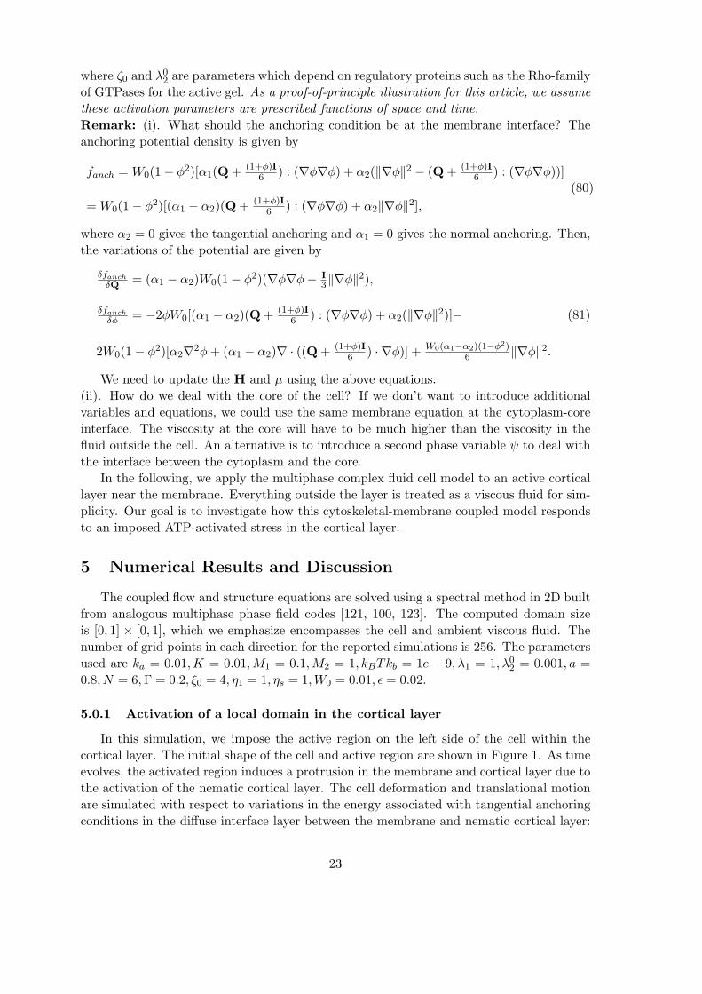
In this simulation, we impose the active region on the left side of the cell within the
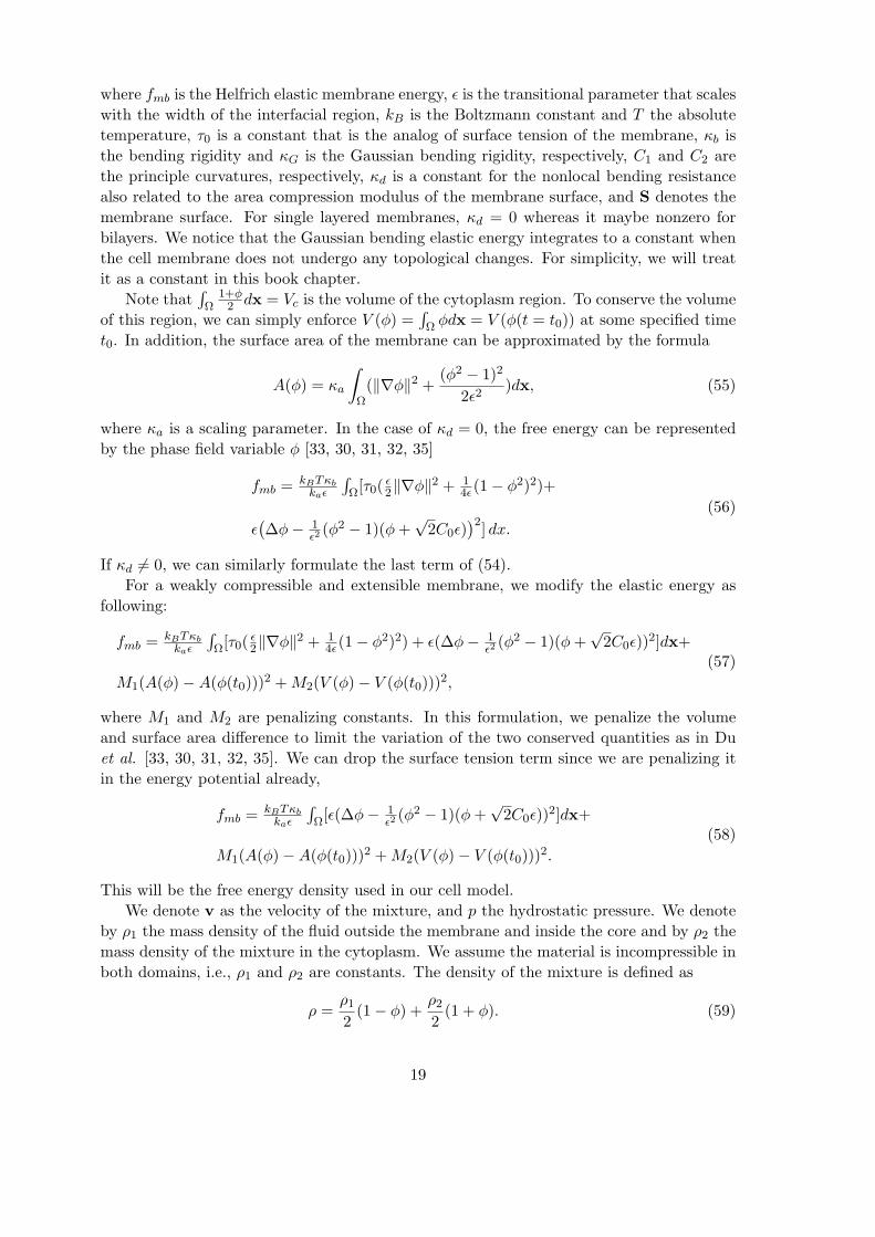
cortical layer. The initial shape of the cell and active region are shown in Figure 1. As time
evolves, the activated region induces a protrusion in the membrane and cortical layer due to
the activation of the nematic cortical layer. The cell deformation and translational motion
are simulated with respect to variations in the energy associated with tangential anchoring
conditions in the diffuse interface layer between the membrane and nematic cortical layer:
23
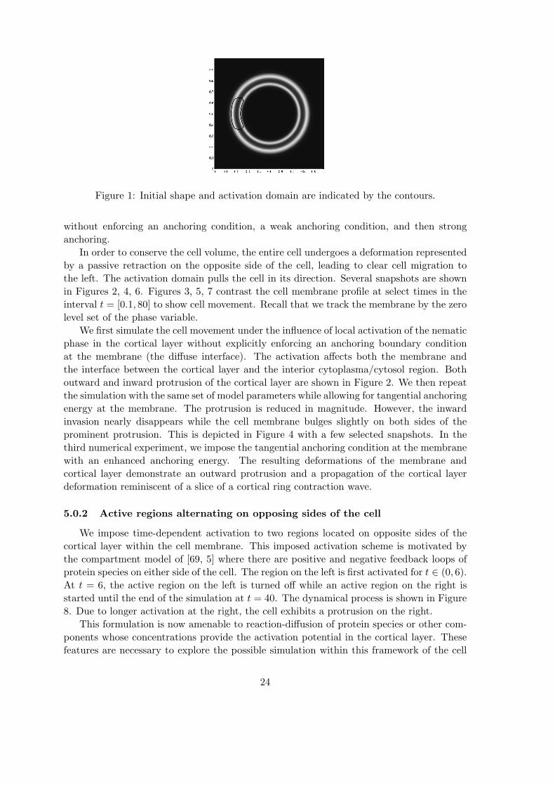
Figure 1: Initial shape and activation domain are indicated by the contours.
without enforcing an anchoring condition, a weak anchoring condition, and then strong
anchoring.
In order to conserve the cell volume, the entire cell undergoes a deformation represented
by a passive retraction on the opposite side of the cell, leading to clear cell migration to
the left. The activation domain pulls the cell in its direction. Several snapshots are shown
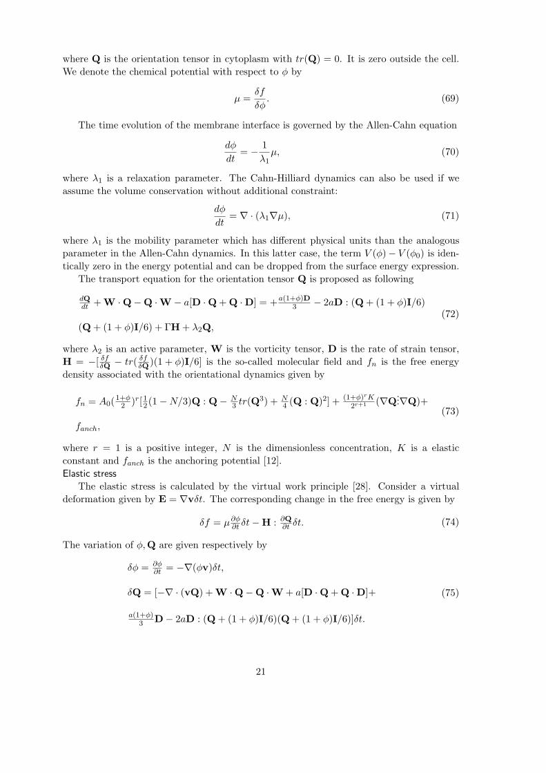
in Figures 2, 4, 6. Figures 3, 5, 7 contrast the cell membrane profile at select times in the
interval t = [0.1, 80] to show cell movement. Recall that we track the membrane by the zero
level set of the phase variable.
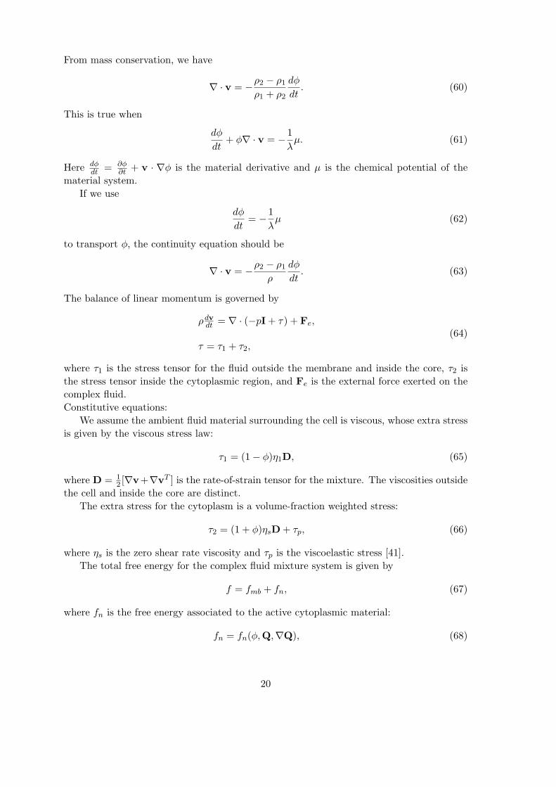
We first simulate the cell movement under the influence of local activation of the nematic
phase in the cortical layer without explicitly enforcing an anchoring boundary condition
at the membrane (the diffuse interface). The activation affects both the membrane and
the interface between the cortical layer and the interior cytoplasma/cytosol region. Both
outward and inward protrusion of the cortical layer are shown in Figure 2. We then repeat
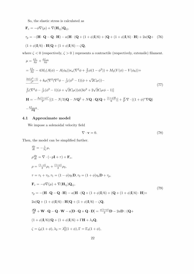
the simulation with the same set of model parameters while allowing for tangential anchoring
energy at the membrane. The protrusion is reduced in magnitude. However, the inward
invasion nearly disappears while the cell membrane bulges slightly on both sides of the
prominent protrusion. This is depicted in Figure 4 with a few selected snapshots. In the
third numerical experiment, we impose the tangential anchoring condition at the membrane
with an enhanced anchoring energy. The resulting deformations of the membrane and
cortical layer demonstrate an outward protrusion and a propagation of the cortical layer
deformation reminiscent of a slice of a cortical ring contraction wave.
5.0.2 Active regions alternating on opposing sides of the cell
We impose time-dependent activation to two regions located on opposite sides of the
cortical layer within the cell membrane. This imposed activation scheme is motivated by
the compartment model of [69, 5] where there are positive and negative feedback loops of
protein species on either side of the cell. The region on the left is first activated for t ∈ (0, 6).
At t = 6, the active region on the left is turned off while an active region on the right is
started until the end of the simulation at t = 40. The dynamical process is shown in Figure
8. Due to longer activation at the right, the cell exhibits a protrusion on the right.
This formulation is now amenable to reaction-diffusion of protein species or other com-
ponents whose concentrations provide the activation potential in the cortical layer. These
features are necessary to explore the possible simulation within this framework of the cell
24
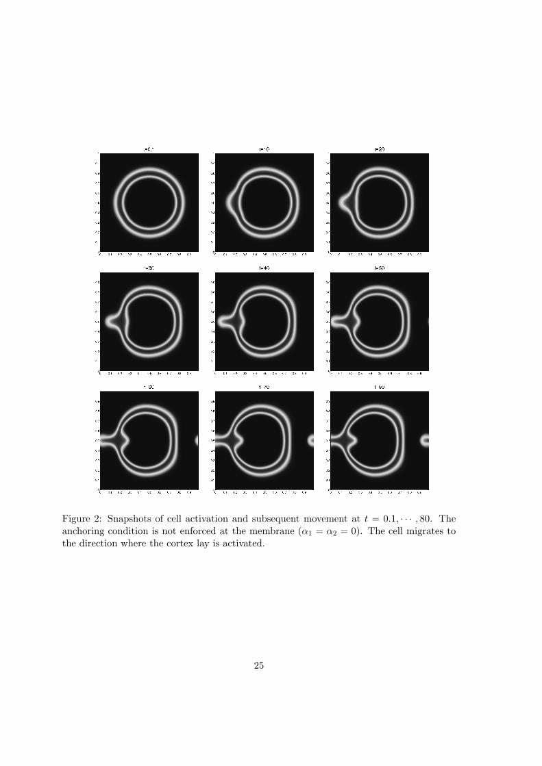
Figure 2: Snapshots of cell activation and subsequent movement at t = 0.1, · · · , 80. Theanchoring condition is not enforced at the membrane (α1 = α2 = 0). The cell migrates tothe direction where the cortex lay is activated.
25
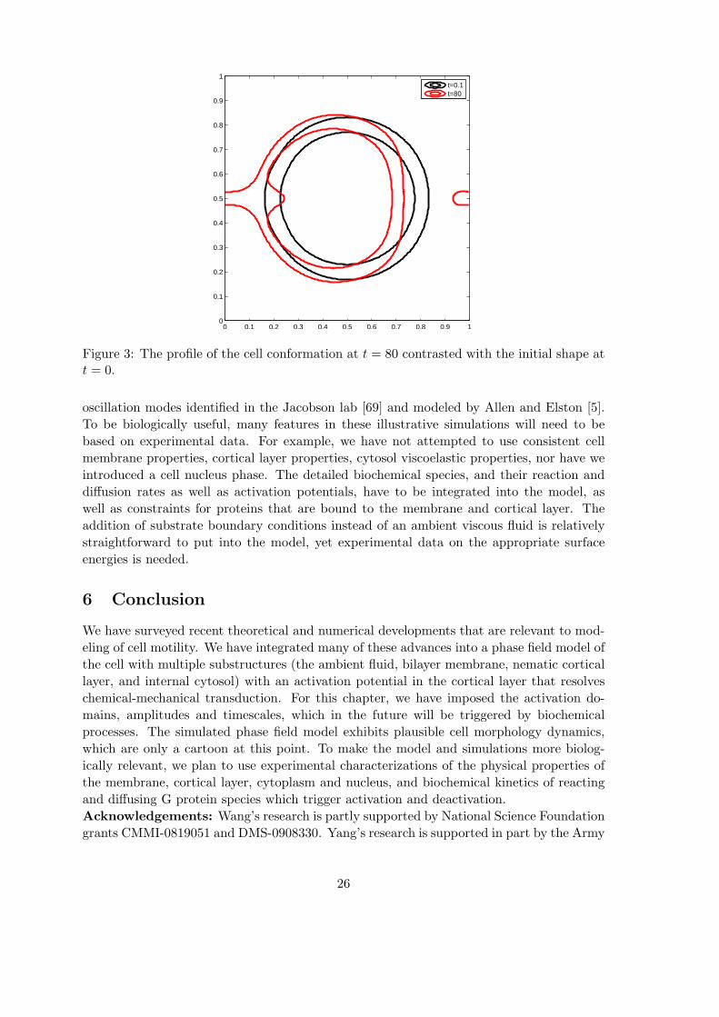
0 0.1 0.2 0.3 0.4 0.5 0.6 0.7 0.8 0.9 10
0.1
0.2
0.3
0.4
0.5
0.6
0.7
0.8
0.9
1t=0.1t=80
Figure 3: The profile of the cell conformation at t = 80 contrasted with the initial shape att = 0.
oscillation modes identified in the Jacobson lab [69] and modeled by Allen and Elston [5].
To be biologically useful, many features in these illustrative simulations will need to be
based on experimental data. For example, we have not attempted to use consistent cell
membrane properties, cortical layer properties, cytosol viscoelastic properties, nor have we
introduced a cell nucleus phase. The detailed biochemical species, and their reaction and
diffusion rates as well as activation potentials, have to be integrated into the model, as
well as constraints for proteins that are bound to the membrane and cortical layer. The
addition of substrate boundary conditions instead of an ambient viscous fluid is relatively
straightforward to put into the model, yet experimental data on the appropriate surface
energies is needed.
6 Conclusion
We have surveyed recent theoretical and numerical developments that are relevant to mod-
eling of cell motility. We have integrated many of these advances into a phase field model of
the cell with multiple substructures (the ambient fluid, bilayer membrane, nematic cortical
layer, and internal cytosol) with an activation potential in the cortical layer that resolves
chemical-mechanical transduction. For this chapter, we have imposed the activation do-
mains, amplitudes and timescales, which in the future will be triggered by biochemical
processes. The simulated phase field model exhibits plausible cell morphology dynamics,
which are only a cartoon at this point. To make the model and simulations more biolog-
ically relevant, we plan to use experimental characterizations of the physical properties of
the membrane, cortical layer, cytoplasm and nucleus, and biochemical kinetics of reacting
and diffusing G protein species which trigger activation and deactivation.
Acknowledgements: Wang’s research is partly supported by National Science Foundation
grants CMMI-0819051 and DMS-0908330. Yang’s research is supported in part by the Army
26
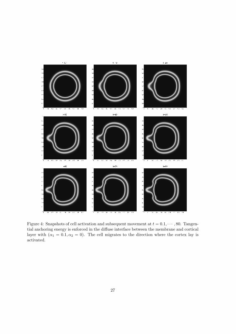
Figure 4: Snapshots of cell activation and subsequent movement at t = 0.1, · · · , 80. Tangen-tial anchoring energy is enforced in the diffuse interface between the membrane and corticallayer with (α1 = 0.1, α2 = 0). The cell migrates to the direction where the cortex lay isactivated.
27

0 0.1 0.2 0.3 0.4 0.5 0.6 0.7 0.8 0.9 10
0.1
0.2
0.3
0.4
0.5
0.6
0.7
0.8
0.9
1t=0.1t=80
Figure 5: The profile of the cell conformation at t = 80 contrasted with the initial shape att = 0.1 for tangential membrane-cortical layer anchoring energy with α1 = 0.1, α2 = 0.
Research Office (ARO) W911NF-09-1-0389. Forest’s research is supported in part by grants
NSF DMS-0908423 and DMS-0943851.
References
[1] D. Adalsteinsson, T. Elston, www.amath.unc.edu/faculty/Adalsteinsson
[2] W. Alt and M. Dembo, Cytoplasm dynamics and cell motion: two-phase fluid models,
Mathematical Biosciences, 156 (1999), 207-228.
[3] E. Atilgan, D. Wirtz and S. X. Sun, Mechanics and Dynamics of Actin-Driven Thin
Membrane Protrusions, Biophysical Journal, 80 (2006), 65-76.
[4] A. Ahmadi, M. C. Marchetti and T. B. Liverpool, Hydrodynamics of isotropic and
liquid crystalline active polymer solutions, Phys. Rev. E, 74 (2006), 061913.
[5] R. Allen and T. Elston, A compartment model for chemically activated, sustained
cellular oscillations, UNC Preprint, 2011.
[6] T. Auth, S. Safran, and N. Gov, Filament networks attached to membranes: cytoskele-
tal pressure and local bilayer deformation, New Journal of Physics, 9 (2007), 430-444.
[7] S. Banerjee and M. C. Marchetti, Instability and oscillations in isotropic gels, Soft
Matter, 7 (2011), 463-473.
[8] T. Baumgart, S. Hess and W. Webb, Imaging coexisting fluid domains in biomembrane
models coupling curvature and line tension, Nature, 425 (2003), 821-824.
[9] A. Baskaran and M. C. Marchetti, Hydrodynamics of self-propelled hard rods, Phys.
Rev. E, 77 (2008), 031311.
28

Figure 6: Snapshots of cell activation and subsequent movement at t = 0.1, · · · , 80.Tangential anchoring energy is enforced in the membrane-cortical layer diffuse interface(α1 = 0.5, α2 = 0). The cell migrates to the direction where the cortex lay is activated.
29
0 0.1 0.2 0.3 0.4 0.5 0.6 0.7 0.8 0.9 10
0.1
0.2
0.3
0.4
0.5
0.6
0.7
0.8
0.9
1t=1t=8
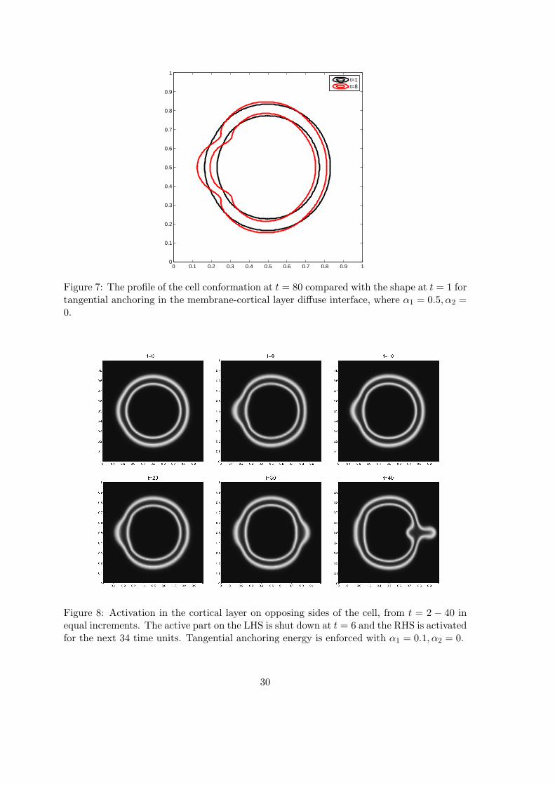
Figure 7: The profile of the cell conformation at t = 80 compared with the shape at t = 1 fortangential anchoring in the membrane-cortical layer diffuse interface, where α1 = 0.5, α2 =0.
Figure 8: Activation in the cortical layer on opposing sides of the cell, from t = 2 − 40 inequal increments. The active part on the LHS is shut down at t = 6 and the RHS is activatedfor the next 34 time units. Tangential anchoring energy is enforced with α1 = 0.1, α2 = 0.
30
[10] A. Baskaran and M. C. Marchetti, Nonequilibrium statistical mechanics of self-
propelled hard rods, Journal of Statistical Mechanics: Theory and Experiment, 4
(2010), 04019.
[11] A. Besser and U. S. Schwarz, Coupling biochemistry and mechanics in cell adhesion:
a model for inhomogeneous stress fiber contraction, New Journal of Physics, 9 (2007),
425.
[12] B. Bird, R. Armstrong and O. Hassager, Dynamics of Polymeric Liquids, 2nd Ed., Vol.
2, John Wiley and Sons, New York, 1987.
[13] A. Bershadsky, M. Kozlov and B. Geiger, Adhesion-mediated mechanosensitivity: a
time to experiment, and a time to theorize, Current Opinion in Cell Biology, 18(2006),
472-481.
[14] D. Boal, Mechanics of the Cell, Cambridge University Press, New York, 2002.
[15] A. Carlsson, Growth velocities of branched actin networks, Biophys. J., 84(2003), 2907-
2918.
[16] M. E. Cates, S. M. Fielding, D. Marenduzzo, E. Orlandini, and J. M. Yeomans, Shear-
ing active gels close to the isotropic-nematic transition, Phys. Rev. Lett., 101(2008),
068102.
[17] A. Kataoka, B. C. W. Tanner, J. M. Macpherson, X. Xu, Q. Wang, M. Reginier, T.
Daniel, and P. B. Chase, Spatially explicit, nanomechanical models of the muscle half
sarcomere: Implications for mechanical tuning in atrophy and fatigue, Acta Astronau-
tica, 60(2)(2007), 111-118.
[18] C. Chen, M. Ren, A. Srinivasan and Q. Wang, 3-D simulations of biofilm-solvent
interaction, Asian Journal of Applied Mathematics, in press, 2011.
[19] L. Q. Chen and W. Yang, Computer simulation of the dynamics of a quenched system
with large number of non-conserved order parameters, Phys. Rev. B, 50(1994), 15752-
15756.
[20] L. Q. Chen, Phase-field modeling for microstructure evolution, Annu. Rev. Mater. Res.,
32(2002), 113-140.
[21] L. Q. Chen and Y. Wang, The continuum field approach to modeling microstructural
evolution, J. Miner Met. Mater. Soc., 48(1996),13-18.
[22] Costigliola, N., Kapustina, M., G. Weinreb, A. Monteith, Z. Rajfur, T. Elston, and K.
Jacobson, Rho regulates calcium independent periodic contractions of the cell cortex,
Biophys. J., 99(4)(2010), 1053–1063.
[23] Z. Cui and Q. Wang, Dynamics of chiral active liquid crystal polymers, DCDS-B,
15(1)(2011), 45-60.
[24] A. Curtis and C. Wilkinson, Nanotechniques and approaches in biotechnology, Trends
Biotechnol, 19(2001), 97-101.
31
[25] P. G. De-Gennes and J. Prost, The Physics of Liquid Crystals, Oxford Science Publi-
cations, Oxford, 1993.
[26] K. A. DeMali, C. A. Barlow and K. Burridge, Recruitment of the Arp2/3 complex to
vinculin: coupling membrane protrusion to matrix adhesion, J. Cell Biol., 159(2002),
881-891.
[27] V. S. Deshpande, R. M. McMeeking, and A. G. Evans, A model for the contractibil-
ity of the cytoskeleton inclduing the effects of stress-fiber formation and dissociation,
Proceedings of the Royal Society A, 463(2007), 787-815.
[28] M. Doi and S. F. Edwards, The Theory of Polymer Dynamics, Oxford University Press,
Oxford, 1986.
[29] G. J. Doherty and H. T. McMahon, Mediation, modulation, and consequences of
membrane-cytoskeleton interactions, Annu. Rev. Biophys., 37(2008), 65-95.
[30] Q. Du, C. Liu, R. Ryham and X. Wang, Phase field modeling of the spontaneous
curvature effect in cell membranes, Comm. Pur. Applied. Anal., 4(2005), 537-548.
[31] Q. Du, C. Liu, R. Ryham and X. Wang, A phase field formulation of the Willmore
problem, Nonlinearity, 18(2005), 1249-1267.
[32] Q. Du, C. Liu, R. Ryham and X. Wang, Energetic variational approaches in modeling
vesicle and fluid interactions, Physica D, 238 (2009), 923-930
[33] Q. Du, C. Liu and X. Wang, A Phase Field Approach in the Numerical Study of the
Elastic Bending Energy for Vesicle Membranes, J. Comp. Phy., 198(2004), 450-468.
[34] Q. Du, C. Liu and X. Wang, Retrieving topological information for phase field models,
SIAM Journal on Applied Mathematics, 65(2005), 1913-1932.
[35] Q. Du, C. Liu and X. Wang, Simulating the Deformation of Vesicle Membranes under
Elastic Bending Energy in Three Dimensions, J. Comp. Phys., 212(2006), 757-777.
[36] C. M. Funkhouser, F. J. Solis and K. Thornton, Coupled composition-deformation
phase-field method for multicomponent lipid membranes, Phys. Rev. E, 76(2007),
011912.
[37] C. M. Funkhouser, F. J. Solis and K. Thornton, Dynamics of two-phase lipid vesicles:
effects of mechanical properties on morphology evolution, Soft Matter, 6(2010), 3462-
466.
[38] X. Wang and Q. Du, Modelling and Simulations of Multi-component Lipid Membranes
and Open Membranes via Diffuse Interface Approaches, J. Math. Biol., 56(2008), 347-
371.
[39] P. A. DiMilla, K. Barbee, and D. Lauffenburger, Mathematical model for the effects of
adhesion and mechanics on cell migration speed, Biophys. J., 60(1991), 15-37.
[40] T. Elston, R. Allen, M. Kapustina, and K. Jacobson, A compartment chemical-
mechanical model for sustained cellular oscillations, University of North Carolina at
Chapel Hill preprint, 2010.
32

[41] M. G. Forest and Q. Wang, Hydrodynamic theories for blends of flexible polymer and
nematic polymers, Physical Review E, 72(2005), 041805.
[42] M. G. Forest, Q. Liao and Q. Wang, 2-D Kinetic Theory for Polymer Particulate
Nanocomposites, Communication in Computational Physics, 7(2)(2010), 250-282.
[43] J. J. Feng, C. Liu, J. Shen and P. Yue, Transient Drop Deformation upon Startup of
Shear in Viscoelastic Fluids, Fluids. Phys. Fluids, 17(2005), 123101.
[44] E. Frixione, Recurring views on the structure and function of the cytoskeleton: a 300-
year epic, Cell motility and the cytoskeleton, 46(2)(2000), 73-94.
[45] A. Gopinathan, K-C Lee, J. M. Schwarz and A. J. Liu, Branching, Capping, and
Severing in Dynamic Actin Structures, Phys. Rev. Lett., 99(2007), 058103.
[46] G. Gerisch, T. Bretschneider, A. Muller-Taubenberger, E. Simmeth, M. Ecke, S. Diez
and K. Anderson, Mobile Actin Clusters and Traveling Waves in Cells Recovering from
Actin Depolymerization, Biophys. J., 87(5)(2004), 3493-3503.
[47] Gregory Giannone, Benjamin J. Dubin-Thaler, Olivier Rossier, Yunfei Cai, Oleg Chaga,
Guoying Jiang, William Beaver, Hans-Gunther Dobereiner, Yoav Freund, Gary Borisy
and Michael P. Sheetz, Lamellipodial Actin Mechanically Links Myosin Activity with
Adhesion-Site Formation, Cell, 128(3)(2007), 561-575.
[48] L. Giomi, T. B. Liverpool, and M. C. Marchetti, Sheared Active Fluids: Thickening,
thinning, and vanishing viscosity, Phys. Rev. E, 81(2010), 051908.
[49] J. L. Guermond, J. Shen, and X. Yang, Error analysis of fully discrete velocity-
correction methods for incompressible flows, Math. Comp., 77(2008), 1387-1405.
[50] Y. Hatwalne, S. Ramaswamy, M. Rao and R. A. Simha, Rheology of Active-Particle
Suspensions, Phys. Rev. Lett., 93(2004), 198105.
[51] R. Hobayashi, Modeling and numerical simulations of dendritic crystal growth, Physica
D, 63 (1993), 410-423.
[52] B. Hoffman and J. Crocker, Cell Mechanics: Dissecting the Physical Responses of Cells
to Force, Annu. Rev. Biomed. Eng., 11(2009), 259-288.
[53] R. Horwitz and J. Parsons, Cell migration-moving on, Science. 286(1999), 1102-3.
[54] R. Horwitz and D. Webb, Cell Migration., Curr Biol., 13(2003), R756-9.
[55] L. Hu and G. A. Papoian, Mechano-Chemical Feedbacks Regulate Actin Mesh Growth
in Lamellipodial Protrusions, Biophys. J., 98(2010), 1375-384.
[56] J. Hua, P. Lin, C. Liu, and Q. Wang, Energy Law Preserving C0 Finite Element
Schemes for Phase Field Models in Two-phase Flow Computations, J. Comp. Phys.,
in press, 2011.
[57] J. Jeong, N. Goldenfeld, and J. Dantzig, Phase field model for three-dimensional den-
dritic growth with fluid flow, Phys. Rev. E, 64(2001), 041602.
33

[58] X. Jiang, S. Takayama, X. Qian, E. Ostuni, H. Wu, N. Bowden, P. LeDuc, D. E. Ingber,
and G. M. Whitesides, Controlling mammalian cell spreading and cytoskeletal arrange-
ment with conveniently fabricated continuous wavy features on poly(dimethylsiloxane),
Langmuir, 18 (2002), 3273-3280.
[59] J. F. Joanny, F. Julicher, and J. Prost, Motion of an Adhesive Gel in a Swelling
Gradient: A Mechanicsm for Cell Locomotion, Phys. Rev. Lett., 25(6) (2003), 168102.
[60] J. F. Joanny, F. Julicher, K. Kruse and J. Prost, Hydrodynamic Theory for Multi-
component Active Polar Gels, New Journal of Physics, 9(2007), 1-17.
[61] F. Julicher, K. Kruse, J. Prost, and J-F. Joanny, Active Behavior of the Cytoskeleton,
Physics Reports, 449(2007), 3-28.
[62] A. Karma and W. Rappel, Phase-field model of dendritic sidebranching with thermal
noise, Phys. Rev. E, 60(1999), 3614-3625.
[63] A. Kataoka, B. C. W. Tanner, J. M. Macpherson, X. Xu, Q. Wang, M. Reginier, T.
Daniel and P. B. Chase, Spatially explicit, nanomechanical models of the muscle half
sarcomere: Implications for mechanical tuning in atrophy and fatigue, Acta Astronau-
tica, 60(2)(2007), 111-118.
[64] D. P. Kiehart and K. Bloom, Cell structure and dynamics, Current Opinion in Cell
Biology, 19(2004), 1-4.
[65] J. Kim and S. Sun, Continuum modeling of forces in growing viscoelastic cytosketal
networks, J. of Theoretical Biology, 256(2009), 596-606.
[66] K. Kruse and F. Julicher, Actively contracting bundles of polar filaments, Phys. Rev.
Lett., 85(8)(2000), 1778-1781.
[67] K. Kruse, J. F. Joanny, F. Julicher, J. Prost and K. Seimoto, Asters, vortices, and
rotating spirals in active gels of polar filaments, Phys. Rev. Lett., 92(7)(2004), 078101.
[68] K. Kruse, J. F. Joanny, F. Julicher, J. Prost, and K. Sekimota, Generic Theory of Active
Polar Gels: A Paradigm for Cytoskeletal Dynamics, Eur. Phys. J. E., 16 (2005), 5-16.
[69] M. Kapustina, G. Weinreb, N. Costigliola, Z. Rajfur, K. Jacobson, and T. Elston, Me-
chanical and Biochemical Modeling of Cortical Oscillations in Spreading Cells, Biophys.
J., 94(12)(2008), 4605-4620.
[70] C. Liu and N. J. Walkington, An Eulerian description of fluids containing visco-
hyperelastic particles, Arch. Rat. Mech. Ana., 159(2001), 229-252.
[71] C. Liu and J. Shen, A phase field model for the mixture of two incompressible fluids
and its approximation by a fourier-spectral method, Physica D, 179(2003), 211-228.
[72] Y. Li, S. Hu, Z. Liu, and L. Q. Chen, Phase-field model of domain structures in
ferroelectric thin films, Appl. Phys. Lett., 78(2001), 3878-3880.
[73] J. Li, M. G. Forest, Q. Wang and R. Zhou, A Kinetic Theory and Benchmark Predic-
tions for Polymer Dispersed, Semi-Flexible Nanorods and Nanoplatelets, Physica D,
240(2011), 114-30.
34
[74] B. Lindley, Q. Wang and T. Zhang, Multicomponent models for biofilm flows, Discrete
and Continuous Dynamic Systems-Series B, 15(2)(2011), 417-456.
[75] T. B. Liverpool and M. C. Marchetti, Bridging the microscopic and the hydrodynamic
in active filament solutions, Europhys. Lett. 69(2005), 846.
[76] T. B. Liverpool and M. C. Marchetti, Hydrodynamics and rheology of active polar
filaments, in Cell Motility, Peter Lenz, ed., Springer, NY, 2007.
[77] W. A. Loesberg, J. te Riet, F. C. M. J. M. van Delft, P. Schoen, C. G. Figdor, S.
Speller, J. J. W. A. van Loon, X. F. Walboomers, and J. A. Jansen, The thresh-
old at which substrate nanogroove dimensions may influence fibroblast alignment and
adhesion, Biomaterials, 28(27)(2007), 3944-3951.
[78] J. Lowengrub and L.Truskinovsky, Quasi-incompressible Cahn-Hilliard fluids and topo-
logical transitions, R. Soc. Lond. Proc. Ser. A Math. Phys. Eng. Sci., 454(1998), 2617-
2654.
[79] W. Lu and Z. Suo, Dynamics of nanoscale pattern formation of an epitaxial monolayer,
J. Mech. Phys. Solids, 49(2001), 1937-1950.
[80] D. Marenduzzo, E. Orlandini, M. E. Cates, and J. M. Yeomans, Steady-state hydro-
dynamic instabilities of active liquid crystals: Hybrid lattice Boltzmann simulations,
Phys. Rev. E, 76 (2007), 031921.
[81] G. McFadden, A. Wheeler, R. Braun, S. Coriell, and R. Sekerka, Phase-field models
for anisotropic interfaces, Phys. Rev. E, 4(1993), 2016-2024.
[82] K. Michie and J. Lowengrub, Dynamic filaments of the bacterial cytoskeleton, Annu.
Rev. Biochem., 75(2006), 467-492.
[83] M. Mofrad and R. Kamm, Cytoskeletal Mechanics: Models and Measurements, Cam-
bridge University Press, 2006.
[84] A. Mogilner, On the edge: modeling protrusion, Current Opinion in Cell Biology,
18(2006), 32-39.
[85] A. Mogilner and L. Edelstein-Keshet, Regulation of Actin Dynamics in Rapidly Moving
Cells: A quantitative Analysis, Biophys. J., 83(2002), 1237-1258.
[86] S. Muhuri, M. Rao, and S. Ramaswamy, Shear Flow Induced Isotropic to Nematic
Transition in A Suspension of Active Filaments, Europhysics Lett., 78(2007), 48002.
[87] J. Murray, Mathematical Biology. Springer-Verlag, Heidelberg, 1989.
[88] L. Nguyen, W. Yang, Q. Wang, and L. Hirst, Molecular dynamics simulation of F-
actin reveals the role of cross-linkers in semi-flexible filament, Soft Matter, 5(2009),
2033-2036.
[89] G. Oster and A. Perelson, Cell spreading and motility: A model lamellipod, Journal
of Mathematical Biology, 21(1985), 383-388.
35

[90] C. Parent and P. Devreotes, A cell’s sense of direction, Science, 284(1999), 765-70.
[91] E. Paluch, M. Piel, and C. Sykes, Cortical actomyosin breakage triggers shape oscilla-
tions in cells and cell fragments, Biophys. J. 89(2005), 724–733.
[92] O. Pletjushkina, Z. Rajfur, P. Pamorski, T. Oliver, J. Vasiliev, and K. Jacobson,
Induction of cortical oscillations in spreading cells by depolymerization of microtubules,
Cell Mot. & Cytoskeleton, 48(4)(2001), 235-244.
[93] T. D. Pollard and G. G. Borisy, Cellular Motility Driven by Assembly and Disassembly
of Actin Filaments, Cell, 112(2003), 453-465.
[94] S. M. Rafelski and J. A. Theriot, Crawling Toward a Unified Model of Cell Motility:
Spatial and Temporal Regulation of Actin Dynamics, Annu. Rev. Biochem., 73(2004),
209-239.
[95] A. J. Ridley, M. A. Schwartz, K. Burridge, R. A. Firtel, M. H. Ginsberg, G. Borisy, J.
T. Parsons, and A. R. Horwitz, Cell migration: integrating signals from front to back,
Science, 302(2003), 1704-1709.
[96] G. Salbreux, J. F. Joanny, J. Prost, and P. Pullarkat, Shape Oscillation of Non-
Adhering Fibroblast Cells, Phys. Biol., (4)(2007), 268-284.
[97] S. Sircar and Q.Wang, Transient rheological responses in sheared biaxial liquid crystals,
Rheological Acta, 49(7)(2010), 699-717.
[98] D. J. Seol, S. Y. Hu, Y. L. Li, J. Shen, K. H. Oh and L. Q. Chen, Three-dimensional
Phase-Field Modeling of Spinodal Decomposition in Constrained Films, Acta Materi-
alia, 51(2003), 5173-5185.
[99] D. Saintillan and M. Shelley, Instabilities and Pattern Formation in Active Particle
Suspensions: Kinetic Theory and Continuum Simulations, Phys. Rev. Lett., 100(2008),
178103.
[100] J. Shen and X. Yang, An efficient moving mesh spectral method for the phase-field
model of two phase flows, J. Comput. Phys., 228(2009), 2978-2992.
[101] Y. L. Shih and L. Rothfield, The bacterial cytoskeleton, Microbiol. Mol. Biol. Rev.,
70(3)(2006), 729-754.
[102] R. A. Simha and S. Ramaswamy, Hydrodynamic Fluctuation and Instabilities in Or-
dered Suspension of Self-Propelled Particles, 89(5)(2002), 058101.
[103] M. R. Stachowiak and B. O’Shaughnessy, Kinetics of stress fibers, New Journal of
Physics, 9(2007), 025002.
[104] A. Stephanou, M. A. J. Chaplain, and P. Tracqui, A mathematical model for the dy-
namics of large membrane deformation of isolated fibroblasts, Bulletin of mathematical
biology, 66(2004), 1119-1154.
[105] A. Stephanou, E. Mylona, M. Chaplain, and P. Tracqui, A computational model of
cell migration coupling the growth of focal adhesions with oscillatory cell pretrusion,
J. of Theoretical Biology, 253(2008), 701-716.
36
[106] E. Tadmor, R. Phillips, and M. Ortiz, Mixed Atomistic and Continuum Models of
Deformation in Solids, Langmuir, 12(1996), 4529-4534.
[107] P. J. Van Haastert and P. N. Devreotes. Chemotaxis: signalling the way forward, Nat.
Rev. Mol. Cell. Biol., 5(8)(2004), 626-634.
[108] M. Vicente-Manzanares, D. J. Webb and A. R. Horwitz, Cell migration at a glance,
J. Cell Sci., 118(2005), 4917-4919.
[109] Q. Wang, W. E, C. Liu, and P. Zhang, Kinetic theories for flows of nonhomogeneous
rodlike liquid crystalline polymers with a nonlocal intermolecular potential, Physical
Review E, 65(5)(2002), 0515041-0515047.
[110] Q. Wang, A hydrodynamic theory of nematic liquid crystalline polymers of different
configurations, Journal of Chemical Physics, 116(2002), 9120-9136.
[111] Q. Wang, M. G. Forest and R. Zhou, A hydrodynamic theory for solutions of non-
homogeneous nematic liquid crystalline polymers with density variations, J. of Fluid
Engineering, 126(2004), 180-188.
[112] Q. Wang and T. Y. Zhang, Kinetic theories for Biofilms, Discrete and Continuous
Dynamic System-Series B, in revision, 2011.
[113] Y. Wang and C. L. Chen, Simulation of microstructure evolution. In Methods in
Materials Research, Ed. E. N. Ksufmann, R. Abbaschian, A. Bocarsly, C. L. Chien, D.
Dollimore, et al., (1999), 2a3.1-2a3.23.
[114] A. Wheeler, G. McFadden, and W. Boettinger, Phase-Field Model for Solidification
of a Eutectic Alloy, Proc. R. Soc., London Ser. A, 452(1996), 495-525.
[115] G. Weinreb, M. Kapustina, K. Jacobson, and T. Elston, In silico hypothesis generation
using casual mapping (CMAP), PLoS ONE, 4(2009), e5378.
[116] S. M. Wise, J. S. Lowengrub, J. S. Kim and W. C. Johnson, Efficient phase-field
simulation of quantum dot formation in a strained heteroepitaxial film, Superlattices
and Microstructures, 36(2004), 293-304.
[117] C. W. Wolgemuth, A. Mogilner, and G. Oster, The hydration dynamics of poly-
electrolyte gels with applications to cell motility and drug delivery, Eur Biophys. J.,
33(2004), 146-158.
[118] C. W. Wolgemuth, Lamellipodial Contractions during Crawling and Spreading, Bio-
phys. J., 89(3)(2005), 1643-1649.
[119] X. Yang, J. Feng, C. Liu and J. Shen, Numerical simulations of jet pinching-off and
drop formation using an energetic variational phase-field method, J. Comput. Phys.,
218(2006), 417-428.
[120] J. J. Young, Cytoskeleton micromechanics: A continuum-microscopic approach, Dis-
sertation in Mathematics, UNC Chapel Hill, advised by S. Mitran, 2010.
37
[121] P. Yue, J. J. Feng, C. Liu, and J. Shen, A diffuse-interface method for simulating
two-phase flows of complex fluids, J. Fluid Mech., 515 (2004), 293-317.
[122] P. Yue, J. J. Feng, C. Liu, and J. Shen, Diffuse-interface simulations of drop coales-
cence and retraction in viscoelastic fluids, J. Non-Newtonian Fluid Mech., 129(2005),
163-176.
[123] X. Yang, M.G. Forest, J. Shen, C. Liu, Shear cell rupture of liquid crystal droplets in
a viscous fluid, J. Non-Newtonian Fluid Mechanics, 166(2011): 487-499.
[124] T. Y. Zhang, N. Cogan, and Q. Wang, Phase Field Models for Biofilms. II. 2-D
Numerical Simulations of Biofilm-Flow Interaction, Communications in Computational
Physics, 4(2008), 72-101.
[125] T. Y. Zhang and Q. Wang, Cahn-Hilliard vs Singular Cahn-Hilliard Equations in
Phase Field Modeling, Comm. Comput. Phys, 7(2)(2010), 362-382.
[126] J. Zhang, S. Das, and Q. Du, A phase field model for vesicle-substrate adhesion, J.
Computational Physics, 228 (2009), 7837-7849.
38
Recommended