Department of Theoretical Geophysics & Mantle DynamicsUniversity of Utrecht, The Netherlands
Computational GeodynamicsFEM for the 1D advection-diffusion eq
Cedric [email protected]
June 23, 2017

1
Content
Introduction
From the strong form to the weak form
Discretisation
C. Thieulot | FEM for the 1D advection-diffusion equation
2
FEM in 1DA simple 1D grid
I domain Ω of length Lx
I 1D grid, nnx nodes, nelx elements
C. Thieulot | FEM for the 1D advection-diffusion equation
3
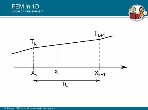
FEM in 1DZoom on one element
C. Thieulot | FEM for the 1D advection-diffusion equation
4
FEM in 1DFrom the strong form to the weak form
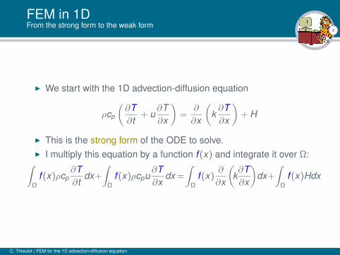
I We start with the 1D advection-diffusion equation
ρcp
(∂T∂t
+ u∂T∂x
)=
∂
∂x
(k∂T∂x
)+ H
I This is the strong form of the ODE to solve.I I multiply this equation by a function f (x) and integrate it over Ω:∫
Ω
f (x)ρcp∂T∂t
dx+
∫Ω
f (x)ρcpu∂T∂x
dx =
∫Ω
f (x)∂
∂x
(k∂T∂x
)dx+
∫Ω
f (x)Hdx
C. Thieulot | FEM for the 1D advection-diffusion equation
5
FEM in 1DFrom the strong form to the weak form
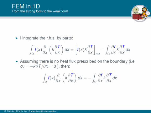
I I integrate the r.h.s. by parts:∫Ω
f (x)∂
∂x
(k∂T∂x
)dx =
[f (x)k
∂T∂x
]∂Ω
−∫
Ω
∂f∂x
k∂T∂x
dx
I Assuming there is no heat flux prescribed on the boundary (i.e.qx = −k∂T/∂x = 0 ), then:∫
Ω
f (x)∂
∂x
(k∂T∂x
)dx = −
∫Ω
∂f∂x
k∂T∂x
dx
C. Thieulot | FEM for the 1D advection-diffusion equation
6
FEM in 1DFrom the strong form to the weak form
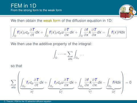
We then obtain the weak form of the diffusion equation in 1D:∫Ω
f (x)ρcp∂T∂t
dx +
∫Ω
f (x)ρcpu∂T∂x
dx +
∫Ω
∂f∂x
k∂T∂x
dx =
∫Ω
f (x)Hdx
We then use the additive property of the integral:∫Ω
· · · =∑elts
∫Ωe
. . .
so that
∑elts
∫
Ωe
fρcp∂T∂t
dx︸ ︷︷ ︸Λe
f
+
∫Ωe
fρcpu∂T∂x
dx︸ ︷︷ ︸Σe
f
+
∫Ωe
∂f∂x
k∂T∂x
dx︸ ︷︷ ︸Υe
f
−∫
Ωe
fHdx︸ ︷︷ ︸Ωe
f
= 0
C. Thieulot | FEM for the 1D advection-diffusion equation
7
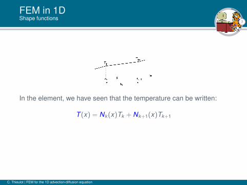
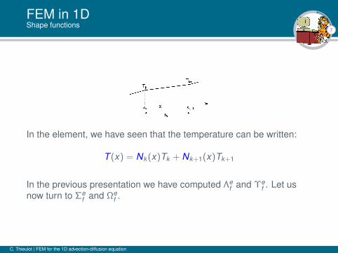
FEM in 1DShape functions
In the element, we have seen that the temperature can be written:
T (x) = Nk (x)Tk + Nk+1(x)Tk+1
In the previous presentation we have computed Λef and Υe
f . Let usnow turn to Σe
f and Ωef .
C. Thieulot | FEM for the 1D advection-diffusion equation
7
FEM in 1DShape functions
In the element, we have seen that the temperature can be written:
T (x) = Nk (x)Tk + Nk+1(x)Tk+1
In the previous presentation we have computed Λef and Υe
f . Let usnow turn to Σe
f and Ωef .
C. Thieulot | FEM for the 1D advection-diffusion equation
8
FEM in 1D.
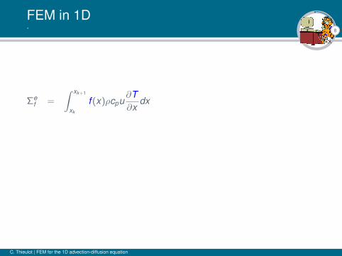
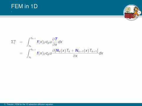
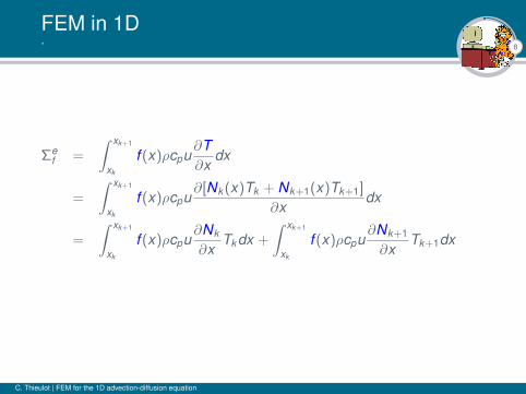
Σef =
∫ xk+1
xk
f (x)ρcpu∂T∂x
dx
=
∫ xk+1
xk
f (x)ρcpu∂[Nk (x)Tk + Nk+1(x)Tk+1]
∂xdx
=
∫ xk+1
xk
f (x)ρcpu∂Nk
∂xTk dx +
∫ xk+1
xk
f (x)ρcpu∂Nk+1
∂xTk+1dx
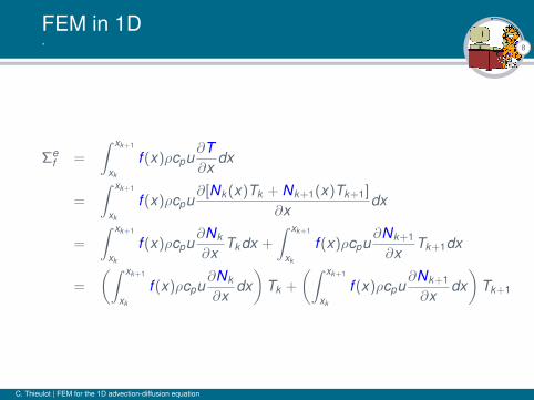
=
(∫ xk+1
xk
f (x)ρcpu∂Nk
∂xdx)
Tk +
(∫ xk+1
xk
f (x)ρcpu∂Nk+1
∂xdx)
Tk+1
C. Thieulot | FEM for the 1D advection-diffusion equation
8
FEM in 1D.
Σef =
∫ xk+1
xk
f (x)ρcpu∂T∂x
dx
=
∫ xk+1
xk
f (x)ρcpu∂[Nk (x)Tk + Nk+1(x)Tk+1]
∂xdx
=
∫ xk+1
xk
f (x)ρcpu∂Nk
∂xTk dx +
∫ xk+1
xk
f (x)ρcpu∂Nk+1
∂xTk+1dx
=
(∫ xk+1
xk
f (x)ρcpu∂Nk
∂xdx)
Tk +
(∫ xk+1
xk
f (x)ρcpu∂Nk+1
∂xdx)
Tk+1
C. Thieulot | FEM for the 1D advection-diffusion equation
8
FEM in 1D.
Σef =
∫ xk+1
xk
f (x)ρcpu∂T∂x
dx
=
∫ xk+1
xk
f (x)ρcpu∂[Nk (x)Tk + Nk+1(x)Tk+1]
∂xdx
=
∫ xk+1
xk
f (x)ρcpu∂Nk
∂xTk dx +
∫ xk+1
xk
f (x)ρcpu∂Nk+1
∂xTk+1dx
=
(∫ xk+1
xk
f (x)ρcpu∂Nk
∂xdx)
Tk +
(∫ xk+1
xk
f (x)ρcpu∂Nk+1
∂xdx)
Tk+1
C. Thieulot | FEM for the 1D advection-diffusion equation
8
FEM in 1D.
Σef =
∫ xk+1
xk
f (x)ρcpu∂T∂x
dx
=
∫ xk+1
xk
f (x)ρcpu∂[Nk (x)Tk + Nk+1(x)Tk+1]
∂xdx
=
∫ xk+1
xk
f (x)ρcpu∂Nk
∂xTk dx +
∫ xk+1
xk
f (x)ρcpu∂Nk+1
∂xTk+1dx
=
(∫ xk+1
xk
f (x)ρcpu∂Nk
∂xdx)
Tk +
(∫ xk+1
xk
f (x)ρcpu∂Nk+1
∂xdx)
Tk+1
C. Thieulot | FEM for the 1D advection-diffusion equation
9
FEM in 1D.
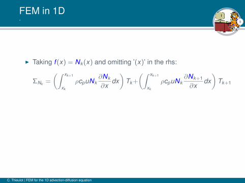
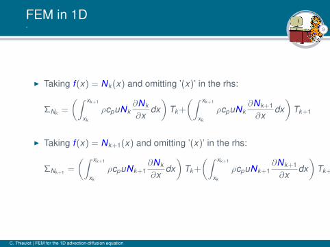
I Taking f (x) = Nk (x) and omitting ’(x)’ in the rhs:
ΣNk =
(∫ xk+1
xk
ρcpuNk∂Nk
∂xdx)
Tk +
(∫ xk+1
xk
ρcpuNk∂Nk+1
∂xdx)
Tk+1
I Taking f (x) = Nk+1(x) and omitting ’(x)’ in the rhs:
ΣNk+1 =
(∫ xk+1
xk
ρcpuNk+1∂Nk
∂xdx)
Tk +
(∫ xk+1
xk
ρcpuNk+1∂Nk+1
∂xdx)
Tk+1
C. Thieulot | FEM for the 1D advection-diffusion equation
9
FEM in 1D.
I Taking f (x) = Nk (x) and omitting ’(x)’ in the rhs:
ΣNk =
(∫ xk+1
xk
ρcpuNk∂Nk
∂xdx)
Tk +
(∫ xk+1
xk
ρcpuNk∂Nk+1
∂xdx)
Tk+1
I Taking f (x) = Nk+1(x) and omitting ’(x)’ in the rhs:
ΣNk+1 =
(∫ xk+1
xk
ρcpuNk+1∂Nk
∂xdx)
Tk +
(∫ xk+1
xk
ρcpuNk+1∂Nk+1
∂xdx)
Tk+1
C. Thieulot | FEM for the 1D advection-diffusion equation
10
FEM in 1D.
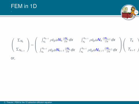
ΣNk
ΣNk+1
=
∫ xk+1
xkρcpuNk
∂Nk∂x dx
∫ xk+1
xkρcpuNk
∂Nk+1∂x dx∫ xk+1
xkρcpuNk+1
∂Nk∂x dx
∫ xk+1
xkρcpuNk+1
∂Nk+1∂x dx
· Tk
Tk+1
or,
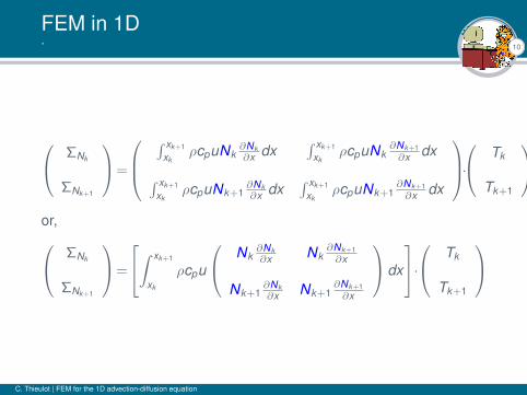
ΣNk
ΣNk+1
=
∫ xk+1
xk
ρcpu
Nk∂Nk∂x Nk
∂Nk+1∂x
Nk+1∂Nk∂x Nk+1
∂Nk+1∂x
dx
· Tk
Tk+1
C. Thieulot | FEM for the 1D advection-diffusion equation
10
FEM in 1D.
ΣNk
ΣNk+1
=
∫ xk+1
xkρcpuNk
∂Nk∂x dx
∫ xk+1
xkρcpuNk
∂Nk+1∂x dx∫ xk+1
xkρcpuNk+1
∂Nk∂x dx
∫ xk+1
xkρcpuNk+1
∂Nk+1∂x dx
· Tk
Tk+1
or, ΣNk
ΣNk+1
=
∫ xk+1
xk
ρcpu
Nk∂Nk∂x Nk
∂Nk+1∂x
Nk+1∂Nk∂x Nk+1
∂Nk+1∂x
dx
· Tk
Tk+1
C. Thieulot | FEM for the 1D advection-diffusion equation
11
FEM in 1D.
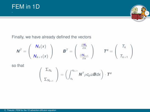
Finally, we have already defined the vectors
NT =
Nk (x)
Nk+1(x)
BT =
∂Nk∂x
∂Nk+1∂x
T e =
Tk
Tk+1
so that ΣNk
ΣNk+1
=
(∫ xk+1
xk
NTρcpuBdx)· T e
C. Thieulot | FEM for the 1D advection-diffusion equation
12
FEM in 1D.
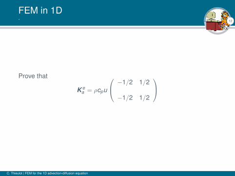
Prove that
K ea = ρcpu
−1/2 1/2
−1/2 1/2
C. Thieulot | FEM for the 1D advection-diffusion equation
13
FEM in 1D
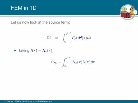
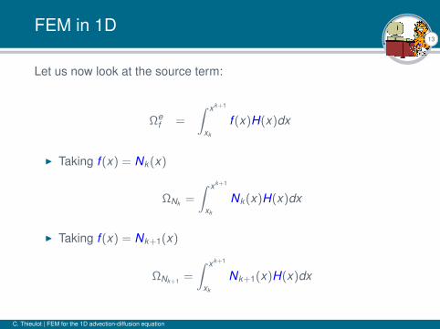
Let us now look at the source term:
Ωef =
∫ xk+1
xk
f (x)H(x)dx
I Taking f (x) = Nk (x)
ΩNk =
∫ xk+1
xk
Nk (x)H(x)dx
I Taking f (x) = Nk+1(x)
ΩNk+1 =
∫ xk+1
xk
Nk+1(x)H(x)dx
C. Thieulot | FEM for the 1D advection-diffusion equation
13
FEM in 1D
Let us now look at the source term:
Ωef =
∫ xk+1
xk
f (x)H(x)dx
I Taking f (x) = Nk (x)
ΩNk =
∫ xk+1
xk
Nk (x)H(x)dx
I Taking f (x) = Nk+1(x)
ΩNk+1 =
∫ xk+1
xk
Nk+1(x)H(x)dx
C. Thieulot | FEM for the 1D advection-diffusion equation
14
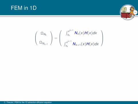
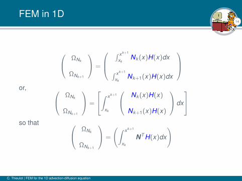
FEM in 1D
ΩNk
ΩNk+1
=
∫ xk+1
xkNk (x)H(x)dx
∫ xk+1
xkNk+1(x)H(x)dx
or, ΩNk
ΩNk+1
=
∫ xk+1
xk
Nk (x)H(x)
Nk+1(x)H(x)
dx
so that ΩNk
ΩNk+1
=
(∫ xk+1
xk
NT H(x)dx
)
C. Thieulot | FEM for the 1D advection-diffusion equation
14
FEM in 1D
ΩNk
ΩNk+1
=
∫ xk+1
xkNk (x)H(x)dx
∫ xk+1
xkNk+1(x)H(x)dx
or, ΩNk
ΩNk+1
=
∫ xk+1
xk
Nk (x)H(x)
Nk+1(x)H(x)
dx
so that ΩNk
ΩNk+1
=
(∫ xk+1
xk
NT H(x)dx
)
C. Thieulot | FEM for the 1D advection-diffusion equation
15
FEM in 1D
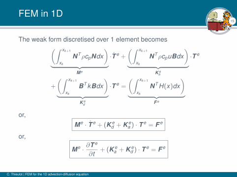
The weak form discretised over 1 element becomes(∫ xk+1
xk
NTρcpNdx)
︸ ︷︷ ︸Me
·T e +
(∫ xk+1
xk
NTρcpuBdx)
︸ ︷︷ ︸K e
a
·T e
+
(∫ xk+1
xk
BT kBdx)
︸ ︷︷ ︸K e
d
·T e =
(∫ xk+1
xk
NT H(x)dx)
︸ ︷︷ ︸F e
or,Me · T e + (K e
d + K ea ) · T e = F e
or,
Me · ∂T e
∂t+ (K e
a + K ed ) · T e = F e
C. Thieulot | FEM for the 1D advection-diffusion equation
16
FEM in 1D
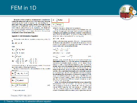
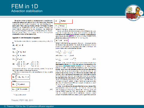
Thieulot, PEPI 188, 2011
C. Thieulot | FEM for the 1D advection-diffusion equation
17
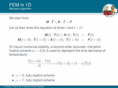
FEM in 1DMid-point algorithm
We start fromM · T + K · T = F
Let us then write this equation at times t and t + δt :
M(t) · T (t) + K (t) · T (t) = F (t)M(t + δt) · T (t + δt) + K (t + δt) · T (t + δt) = F (t + δt)
To insure numerical stability, a second order accurate, mid-pointimplicit scheme (α = 0.5) is used to represent the time derivative oftemperature :
T (t + δt) − T (t)δt
= αT (t + δt) + (1 − α)T (t)
I α = 0: fully explicit schemeI α = 1: fully implicit scheme
C. Thieulot | FEM for the 1D advection-diffusion equation
18
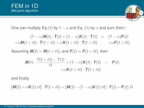
FEM in 1DMid-point algorithm
One can multiply Eq.(1) by 1 − α and Eq. (1) by α and sum them :
(1 − α)M(t) · T (t) + (1 − α)K (t) · T (t) = (1 − α)F (t)+αM(t + δt) · T (t + δt) + αK (t + δt) · T (t + δt) +αF (t + δt)
Assuming M(t) ≈ M(t + δt), and F (t) ≈ F (t + δt), then
M(t) · T (t + δt) − T (t)δt
+ (1 − α)K (t) · T (t) = F (t)
+αK (t + δt) · T (t + δt)
and finally
[M(t) + αK (t) δt ] · T (t + δt) = [M(t) − (1 − α)K (t) δt ] · T (t) + F (t) δt
C. Thieulot | FEM for the 1D advection-diffusion equation
19
FEM in 1DMid-point algorithm
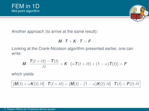
Another approach (to arrive at the same result):
M · T + K · T = F
Looking at the Crank-Nicolson algorithm presented earlier, one canwrite:
M · T (t + δt) − T (t)δt
+ K · (αT (t + δt) + (1 − α)T (t)) = F
which yields
[M(t) + αK (t) δt ] · T (t + δt) = [M(t) − (1 − α)K (t) δt ] · T (t) + F (t) δt
C. Thieulot | FEM for the 1D advection-diffusion equation
20
FEM in 1DAdvection stabilisation
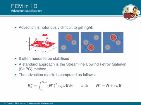
I Advection is notoriously difficult to get right:
I It often needs to be stabilisedI A standard approach is the Streamline Upwind Petrov Galerkin
(SUPG) method.I The advection matrix is computed as follows:
K ea =
∫ xk+1
xk
(N?)TρcpuBdx with N? = N + τuB
C. Thieulot | FEM for the 1D advection-diffusion equation
21
FEM in 1DAdvection stabilisation
Thieulot, PEPI 188, 2011
C. Thieulot | FEM for the 1D advection-diffusion equation
22
FEM in 1DAdvection stabilisation
Prove that in the SUPG case
(K ea )SUPG = K e
a + ρcpτu2
hx
1 −1
−1 1
C. Thieulot | FEM for the 1D advection-diffusion equation
23
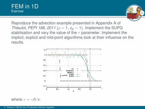
FEM in 1DExercise
Reproduce the advection example presented in Appendix A ofThieulot, PEPI 188, 2011 (ρ = 1, cp = 1). Implement the SUPGstabilisation and vary the value of the τ parameter. Implement theimplicit, explicit and mid-point algorithms look at their influence on theresults.
where τ = γh/v .
C. Thieulot | FEM for the 1D advection-diffusion equation
Recommended