Computed Tomography (CT):Physics and Technology
Clinical Applications
Computed Tomography (CT):Physics and Technology
Clinical Applications
Ontario Cancer InstitutePrincess Margaret HospitalUniversity Health Network
Medical BiophysicsMedical ImagingIBBME
JH Siewerdsen PhD
Dept. of Medical Biophysics, University of TorontoOntario Cancer Institute, Princess Margaret Hospital
JH Siewerdsen PhD
Dept. of Medical Biophysics, University of TorontoOntario Cancer Institute, Princess Margaret Hospital
M O’Malley MD
Dept. of Medical Imaging, University of TorontoDept. of Medical Imaging, University Health Network / Mt. Sinai Hospital
martin.o’[email protected]
M O’Malley MD
Dept. of Medical Imaging, University of TorontoDept. of Medical Imaging, University Health Network / Mt. Sinai Hospital
martin.o’[email protected]
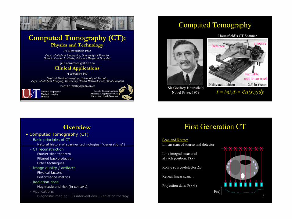
• Computed Tomography (CT)- Basic principles of CT
Natural history of scanner technologies (“generations”)
- CT reconstructionFourier slice theoremFiltered backprojectionOther techniques
- Image quality / artifactsPhysical factorsPerformance metrics
- Radiation doseMagnitude and risk (in context)
- ApplicationsDiagnostic imaging… IG interventions… Radiation therapy
OverviewOverview
Circa 1895
Projection radiography I0
I
I = Io e-∫µ(x,y)dy0
d
Computed Tomography
P = ln(Io/I) = ∫µ(x,y)dySir Godfrey Hounsfield
Nobel Prize, 1979
γ source
9-day acquisition 2.5-hr recon
Detector
Turntableand linear track
Hounsfield’s CT Scanner
First Generation CT
xScan and Rotate:Linear scan of source and detector
Line integral measuredat each position: P(x)
Rotate source-detector ∆θ
Repeat linear scan…
Projection data: P(x;θ)
x x x x x x x
P(x)
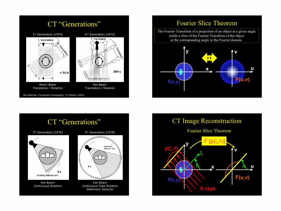
CT “Generations”
WA Kalender, Computed Tomography, 2nd Edition (2005)
1st Generation (1970)
Pencil BeamTranslation / Rotation
2nd Generation (1972)
Fan BeamTranslation / Rotation
CT “Generations”3rd Generation (1976)
Fan BeamContinuous Rotation
4th Generation (1978)
Fan BeamContinuous Tube Rotation
Stationary Detector
The Fourier Transform of a projection of an object at a given angleyields a slice of the Fourier Transform of the objectat the corresponding angle in the Fourier domain.
Fourier Slice Theorem
f(x,y)
y
x
v
u
FT
F(u,v)
CT Image ReconstructionFourier Slice Theorem
v
u
f(x,y)
ξ
θ
y
x
p(ξ,θ)
X-rays
θ
F(u,v)
F [p(ξ,θ)]
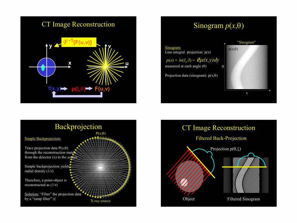
CT Image Reconstruction
y
x
v
u
f(x,y) p(ξ,θ) F(u,v)
F -1[F(u,v)]
BackprojectionSimple Backprojection:
Trace projection data P(x;θ)through the reconstruction matrixfrom the detector (x) to the source
Simple backprojection yieldsradial density (1/r)
Therefore, a point-object isreconstructed as (1/r)
Solution: “Filter” the projection databy a “ramp filter” |r|
P(x;θ)
X-ray source
Sinogram p(x,θ)
Sinogram:Line integral projection: p(x)
measured at each angle (θ)
Projection data (sinogram): p(x;θ)
x
θ
p(x;θ)
“Sinogram”
p(x) = ln(Io/I) = ∫µ(x,y)dy
SinogramFiltered Sinogram
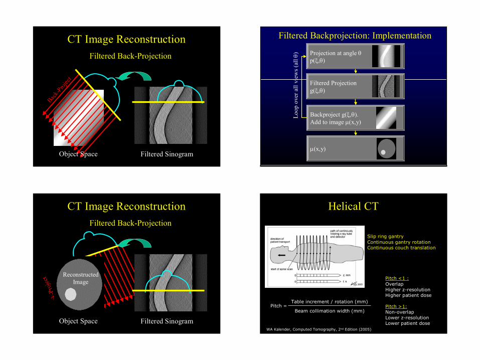
CT Image ReconstructionFiltered Back-Projection
Object
Projection p(θ,ξ)
Back-P
rojec
t
CT Image ReconstructionFiltered Back-Projection
Filtered SinogramObject Space
Back
-Pro
ject
CT Image ReconstructionFiltered Back-Projection
Filtered SinogramObject Space
ReconstructedImage
Filtered Backprojection: Implementation
Projection at angle θp(ξ,θ)
Filtered Projectiong(ξ,θ)
Backproject g(ξ,θ).Add to image µ(x,y)
µ(x,y)
Loop
ove
r all
view
s (al
l θ)
Helical CT
WA Kalender, Computed Tomography, 2nd Edition (2005)
Slip ring gantryContinuous gantry rotationContinuous couch translation
Pitch =Table increment / rotation (mm)
Beam collimation width (mm)
Pitch <1 :OverlapHigher z-resolutionHigher patient dose
Pitch >1:Non-overlapLower z-resolutionLower patient dose
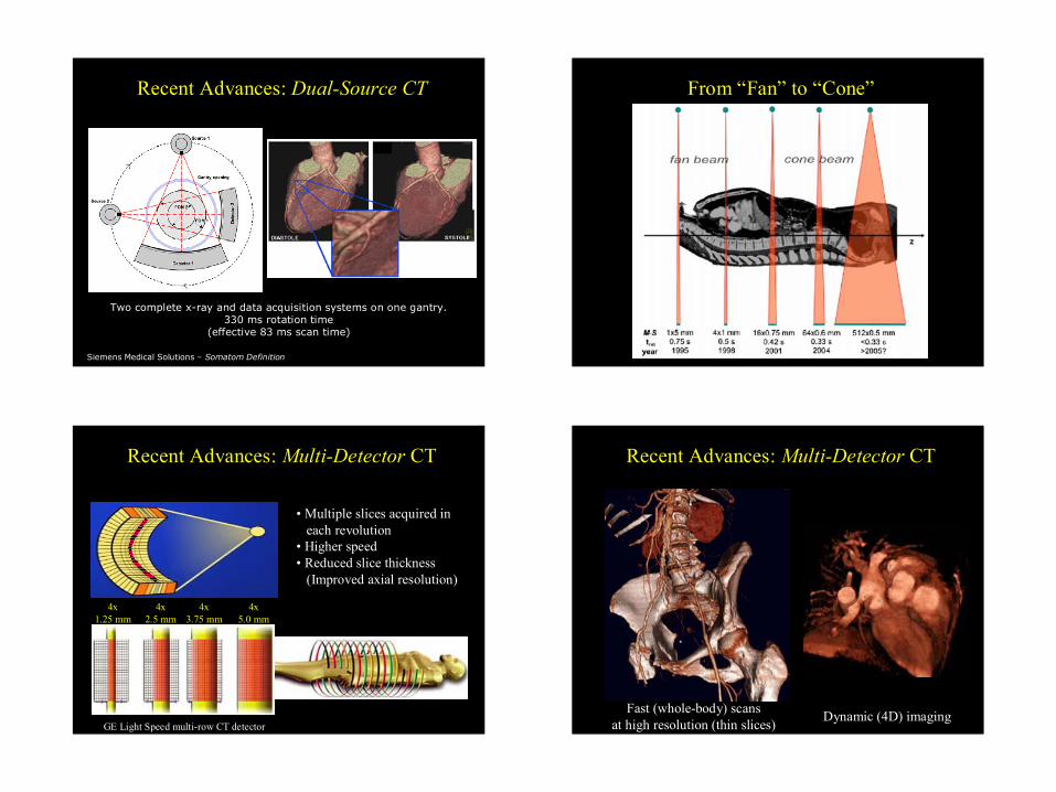
Recent Advances: Dual-Source CT
Two complete x-ray and data acquisition systems on one gantry.330 ms rotation time
(effective 83 ms scan time)
Siemens Medical Solutions – Somatom Definition
Recent Advances: Multi-Detector CT
• Multiple slices acquired in each revolution
• Higher speed• Reduced slice thickness
(Improved axial resolution)
GE Light Speed multi-row CT detector
4x1.25 mm
4x2.5 mm
4x3.75 mm
4x5.0 mm
From “Fan” to “Cone”
Recent Advances: Multi-Detector CT
Fast (whole-body) scansat high resolution (thin slices) Dynamic (4D) imaging
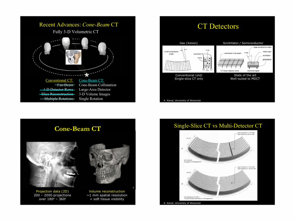
Recent Advances: Cone-Beam CTFully 3-D Volumetric CT
Conventional CT:Fan-Beam
1-D Detector RowsSlice Reconstruction
Multiple Rotations
Cone-Beam CT:Cone-Beam CollimationLarge-Area Detector3-D Volume ImagesSingle Rotation
Cone-Beam CT
Projection data (2D)200 – 2000 projections
over 180o – 360o
Volume reconstruction~1 mm spatial resolution
+ soft tissue visibility
CT Detectors
K. Kanal, University of Wisconsin
Gas (Xenon)
Conventional (old)Single-slice CT only
Scintillator / Semiconductor
State of the artWell-suited to MDCT
Single-Slice CT vs Multi-Detector CT
K. Kanal, University of Wisconsin
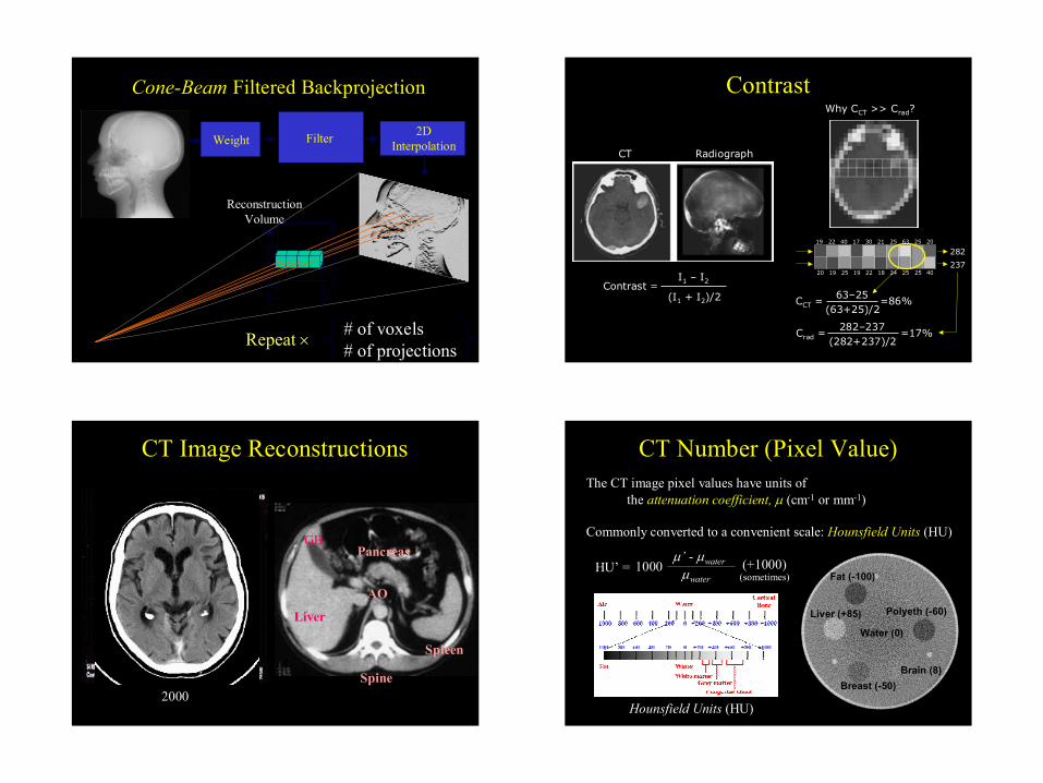
Cone-Beam Filtered Backprojection
Weight Filter 2D Interpolation
Geometry
# of voxels# of projectionsRepeat ×
Reconstruction Volume
CT Image Reconstructions
1975
Liver
GB
Spine
Spleen
AO
Pancreas
2000
282
237
Contrast
Contrast =I1 – I2
(I1 + I2)/2
CT Radiograph
6325 25
252524182219251920 40
20214022 17 3019
Why CCT >> Crad?
CCT =63–25
(63+25)/2=86%
Crad =282–237
(282+237)/2=17%
CT Number (Pixel Value)
Hounsfield Units (HU)
The CT image pixel values have units ofthe attenuation coefficient, µ (cm-1 or mm-1)
Commonly converted to a convenient scale: Hounsfield Units (HU)
HU’ = µ’ - µwaterµwater
1000 (+1000)(sometimes)
Brain (8)
Fat (-100)
Liver (+85)
Breast (-50)
Water (0)
Polyeth (-60)
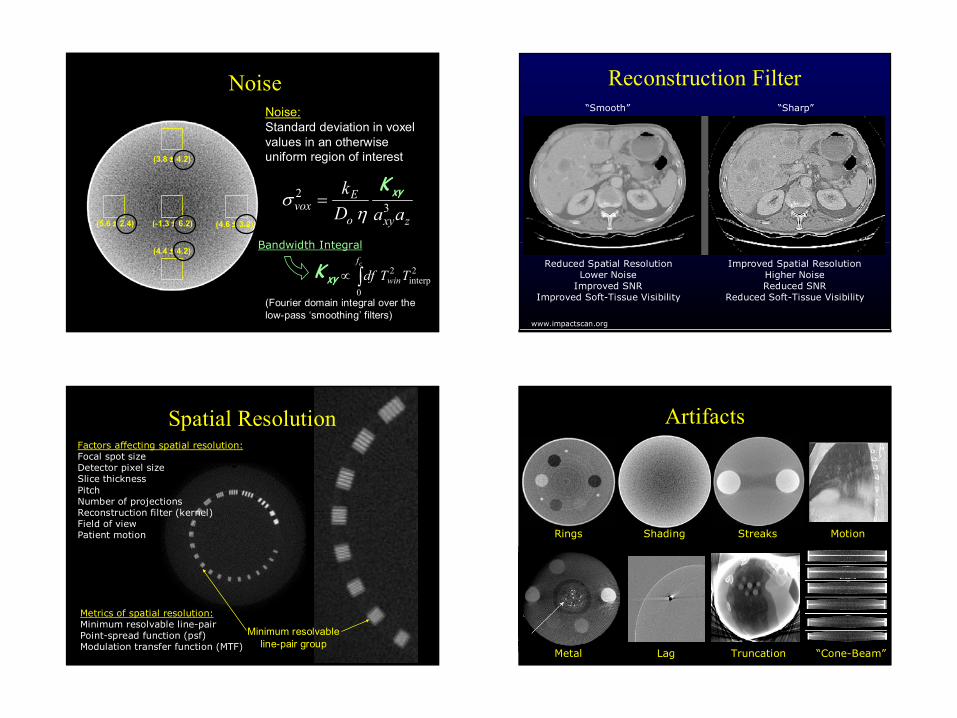
NoiseNoise:Standard deviation in voxelvalues in an otherwise uniform region of interest
(4.6 ± 3.2)(5.6 ± 2.4) (-1.3 ± 6.2)
(3.8 ± 4.2)
(4.4 ± 4.2)
∫∝cf
winTTdf0
2interp
2
Bandwidth Integral
xyK
zxyo
Evox aaD
k3
2
ησ = xyK
(Fourier domain integral over the low-pass ‘smoothing’ filters)
Minimum resolvableline-pair group
Spatial ResolutionFactors affecting spatial resolution:Focal spot sizeDetector pixel sizeSlice thicknessPitchNumber of projectionsReconstruction filter (kernel)Field of viewPatient motion
Metrics of spatial resolution:Minimum resolvable line-pairPoint-spread function (psf)Modulation transfer function (MTF)
www.impactscan.org
“Smooth” “Sharp”
Reconstruction Filter
Reduced Spatial ResolutionLower Noise
Improved SNRImproved Soft-Tissue Visibility
Improved Spatial ResolutionHigher NoiseReduced SNR
Reduced Soft-Tissue Visibility
Artifacts
Rings Shading
Lag
Motion
Metal
Streaks
“Cone-Beam”Truncation
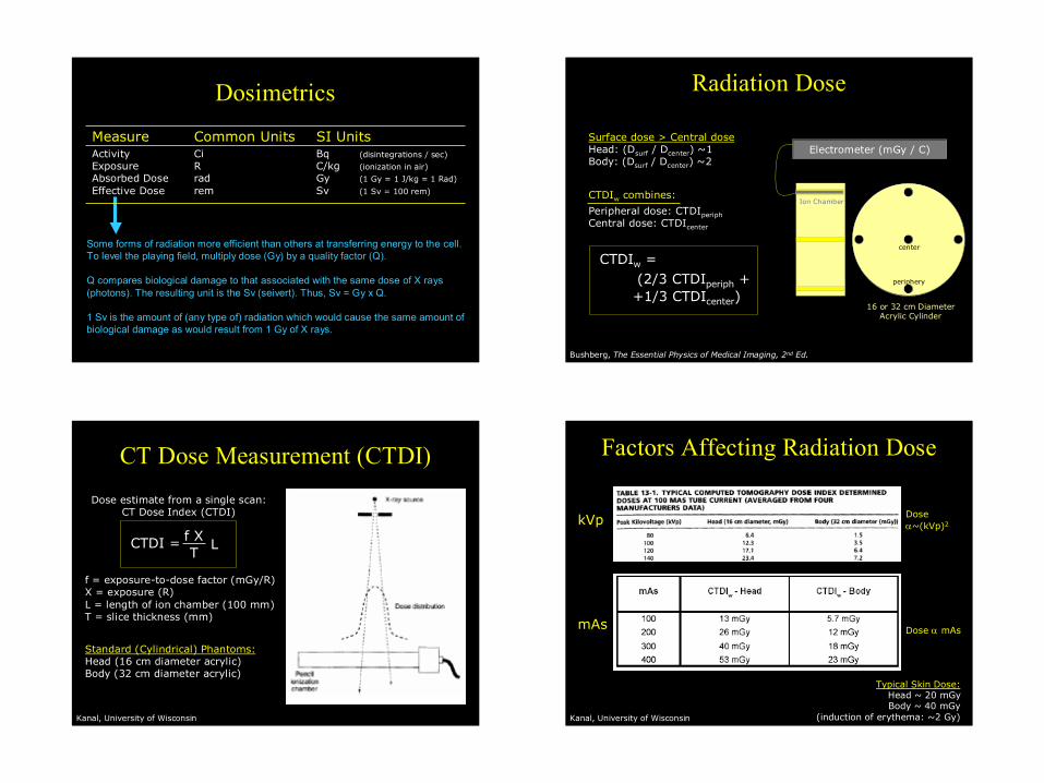
Dosimetrics
Measure Common Units SI UnitsActivity Ci Bq (disintegrations / sec)
Exposure R C/kg (ionization in air)
Absorbed Dose rad Gy (1 Gy = 1 J/kg = 1 Rad)
Effective Dose rem Sv (1 Sv = 100 rem)
Some forms of radiation more efficient than others at transferring energy to the cell.To level the playing field, multiply dose (Gy) by a quality factor (Q).
Q compares biological damage to that associated with the same dose of X rays (photons). The resulting unit is the Sv (seivert). Thus, Sv = Gy x Q.
1 Sv is the amount of (any type of) radiation which would cause the same amount of biological damage as would result from 1 Gy of X rays.
CT Dose Measurement (CTDI)
Kanal, University of Wisconsin
Dose estimate from a single scan:CT Dose Index (CTDI)
CTDI = f XT
L
f = exposure-to-dose factor (mGy/R)X = exposure (R)L = length of ion chamber (100 mm)T = slice thickness (mm)
Standard (Cylindrical) Phantoms:Head (16 cm diameter acrylic)Body (32 cm diameter acrylic)
Radiation Dose
Bushberg, The Essential Physics of Medical Imaging, 2nd Ed.
CTDIw =
Surface dose > Central doseHead: (Dsurf / Dcenter) ~1Body: (Dsurf / Dcenter) ~2
CTDIw combines:
Peripheral dose: CTDIperiphCentral dose: CTDIcenter
(2/3 CTDIperiph ++1/3 CTDIcenter)
Electrometer (mGy / C)
Ion Chamber
16 or 32 cm DiameterAcrylic Cylinder
center
periphery
Factors Affecting Radiation Dose
Typical Skin Dose:Head ~ 20 mGyBody ~ 40 mGy
(induction of erythema: ~2 Gy)
kVp
mAs
Kanal, University of Wisconsin
Doseα~(kVp)2
Dose α mAs
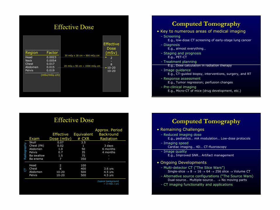
Effective Dose
Region FactorHead 0.0023Neck 0.0054Chest 0.017Abdomen 0.015Pelvis 0.019
(mSv/mGy.cm)
30 mGy x 30 cm = 900 mGy.cm
EffectiveDose
(mSv)2-8
10-2010-20
20 mGy x 50 cm = 1000 mGy.cm
Effective Dose
ExamSkullChest (PA)AbdomenPelvisBa swallowBa enema
HeadChestAbdomenPelvis
EffectiveDose (mSv)
0.070.021.00.71.57
28
10-2010-20
Equivalent# CXR
3.51503575350
100400500500
Approx. PeriodBackroundRadiation
-3 days
6 months4 months
--
3.6 yrs4.5 yrs4.5 yrs
(typical background= 3 mSv / yr)
Rad
iogra
phy
CT
• Key to numerous areas of medical imaging- Screening
E.g., low-dose CT screening of early-stage lung cancer
- DiagnosisE.g., almost everything…
- Staging and prognosisE.g., PET-CT
- Treatment planningE.g., Dose calculation in radiation therapy
- Image guidanceE.g., CT-guided biopsy, interventions, surgery, and RT
- Response assessmentE.g., Tumor regression; perfusion changes
- Pre-clinical imagingE.g., Micro-CT of mice (drug development, etc.)
Computed TomographyComputed Tomography
• Remaining Challenges- Reduced imaging dose
E.g., pediatrics… mA modulation… Low-dose protocols
- Imaging speedCardiac imaging… 4D… CT-fluoroscopy
- Image qualityE.g., Improved SNR… Artifact management
Computed TomographyComputed Tomography
• Ongoing Developments- Multi-detector CT (“The Slice Wars”)
Single-slice → 8 → 16 → 64 → 256 slice → Volume CT
- Alternative source configurations (“The Source Wars)Dual-source… Multiple-source… → No moving parts
- CT imaging functionality and applications
Recommended


![Fundamentals of cone beam computed tomography for a ...Cone beam computed tomography (CBCT, also referred to as C-arm computed tomography [CT], cone beam volume CT, or flat panel CT)](https://img.pdfslide.net/doc/110x75/611ad245d6c77f53c63c9117/fundamentals-of-cone-beam-computed-tomography-for-a-cone-beam-computed-tomography.jpg)