Computer Aided Detection of Transient InflationEvents at Alaskan Volcanoes using GPS Measurements
from 2005-2015
Justin D Lialowast Cody M Rudea David M Blaira Michael G GowanlockaThomas A Herringb Victor Pankratiusa
aAstro-ampGeo-Informatics Group MIT Haystack Observatory Westford MA USAbDepartment of Earth Atmospheric and Planetary Sciences MIT Cambridge MA USA
Abstract
Analysis of transient deformation events in time series data observed via net-works of continuous Global Positioning System (GPS) ground stations provideinsight into the magmatic and tectonic processes that drive volcanic activityTypical analyses of spatial positions originating from each station require care-ful tuning of algorithmic parameters and selection of time and spatial regionsof interest to observe possible transient events This iterative manual processis tedious when attempting to make new discoveries and does not easily scalewith the number of stations Addressing this challenge we introduce a novelapproach based on a computer-aided discovery system that facilitates the dis-covery of such potential transient events The advantages of this approach aredemonstrated by actual detections of transient deformation events at volcanoesselected from the Alaska Volcano Observatory database using data recorded byGPS stations from the Plate Boundary Observatory network Our techniquesuccessfully reproduces the analysis of a transient signal detected in the firsthalf of 2008 at Akutan volcano and is also directly applicable to 3 additionalvolcanoes in Alaska with the new detection of 2 previously unnoticed infla-tion events in early 2011 at Westdahl and in early 2013 at Shishaldin Thisstudy also discusses the benefits of our computer-aided discovery approach forvolcanology in general Advantages include the rapid analysis on multi-scaleresolutions of transient deformation events at a large number of sites of interestand the capability to enhance reusability and reproducibility in volcano studies
Keywords Alaska Volcanoes Transient Inflation Events GPSComputer-Aided Discovery
lowastCorresponding authorEmail address jdlihaystackmitedu (Justin D Li)
Preprint submitted to Journal of Volcanology and Geothermal Research September 12 2016
1 Introduction1
Volcanology has greatly benefited from continued advances in sensor net-2
works that are deployed on volcanoes for continuous monitoring of various3
activities and events over extended periods of time Currently the scientific4
community is expanding and enhancing such sensor networks to improve their5
spatial and temporal resolutions thus creating new opportunities for conduct-6
ing large scale studies and detecting new events and behaviors (Dzurisin 20067
Ji amp Herring 2011)8
However the increasing amount of data recorded by geodetic instruments9
poses formidable challenges in terms of storage data access and processing10
This trend makes manual detection and analysis of new discoveries increas-11
ingly difficult Large data sets also drive the need for cloud data storage and12
high-performance computing as local machines gradually become less capable13
of handling these computational workloads Therefore more sophisticated com-14
putational techniques and tools are required to address to this challenge15
To expand current toolsets and capabilities in volcanology this article presents16
a computer-aided discovery approach to volcanic time series analysis and event17
detection that helps researchers analyze the ever-increasing volume and number18
of volcanic data sets A key novel contribution of this approach is incorporat-19
ing models of volcanology physics to generate relevant and meaningful results20
We demonstrate its applicability by examining geodetic data from the contin-21
uous Global Positioning System (GPS) network operated by the Plate Bound-22
ary Observatory (PBO httppbounavcoorg) and through the detection and23
analysis of transient events in Alaska24
Our computer-aided discovery system implements a processing pipeline with25
configurable user-definable stages We can then select from a number of algo-26
rithmic choices and allowable ranges for numerical parameters that define dif-27
ferent approaches to volcanic data processing Using these specifications the28
system employs systematic techniques to generate variants of this pipeline to29
identify transient volcanic events Variations in the processing pipeline ndash the30
choice of filters the range of parameters and so forth ndash can highlight or sup-31
press features of a transient event and alter the certainty of its detection As32
the optimum pipeline variant is not usually known a priori and is typically se-33
lected manually a tool that automates this search helps make the discovery34
process more efficient and scalable Additionally once configured these soft-35
ware pipelines can be reused for other data sets ndash either to test and reproduce36
results from past studies or to detect new or previously unknown events37
The article is organized as follows Section 2 introduces the different geodetic38
data sets used in this study and briefly outlines the geographic region of inter-39
est Section 3 describes the idea of a computer-aided framework and the specific40
implementation developed and utilized for this study Section 4 presents the41
detection and validation of three transient deformation events whose physical42
characteristics are discussed in Section 5 along with a discussion of the require-43
ments and advantages of the discovery pipeline Finally Section 6 concludes44
with the contributions of the developed computer aided system and suggestions45
2
for further application and refinements46
2 Geodetic Data47
Continuous GPS position measurements (ldquotime seriesrdquo data) have become48
a particularly useful source of geodetic data in the past several decades with49
millimeter-scale resolution and wide-scale deployment Here we analyze daily50
GPS time series data collected by averaging 24 hours of recorded measurements51
at PBO stations in Alaska between 2005 and 2015 The GPS data are ob-52
tained from the PBO archives as a Level 2 product describing GPS station53
time series positions This data is generated from Geodesy Advancing Geo-54
sciences and EarthScope GPS Analysis Centers at Central Washington Univer-55
sity and New Mexico Institute of Mining and Technology and combined into56
a final derived product by the Analysis Center Coordinator at Massachusetts57
Institute of Technology Locations of Alaskan volcanoes along with logs of moni-58
tored volcanic activity are obtained from the Alaska Volcano Observatory (AVO59
httpavoalaskaedu) and used to provide regions of interest that bound sub-60
sets of the PBO GPS stations61
In addition to the GPS data we also utilize snow cover data from the Na-62
tional Snow and Ice Data Center (NSIDC httpnsidcorg) to address possible63
data corruption due to accumulated snow on GPS antennas which can be sig-64
nificant as shown in Figure 1 This novel data fusion of GPS time series data65
with the NSIDC National Ice Centerrsquos Interactive Multisensor Snow and Ice66
Mapping System Daily Northern Hemisphere Snow and Ice Analysis 4 km Res-67
olution data product (National Ice Center 2008) helps identify stations with68
corrupted data resulting from seasonally occurring errors To reduce the com-69
putational time and complexity we apply a preprocessing step that combines70
NSIDC snow mapping data with the PBO GPS data as a single data product71
which we use in later analyses This data fusion approach takes a first step to-72
wards solving the challenging problem of resolving data corrupted by complex73
snow conditions74
2009 2010 2011 2012 2013 2014minus100
minus50
0
50
100
150
Displacement (mm)
Comparison of Snow and PBO Data
AV29 dN
Snow
No Snow
Figure 1 A comparison of the NSIDC snow cover data overlaid on the PBO data showinghow the NSIDC data can be used to identify regions of high variability and missing PBO dataThe blue points (upper line) mark days with snow and the red points (lower line) mark dayswithout snow at station AV29 with its northward motion plotted for comparison in black
3
3 The Computer-Aided Discovery Pipeline75
We demonstrate the utility of our approach for volcanology by analyzing76
GPS measurements of displacements near and at volcanoes in Alaska between77
2005 and 2015 We evaluate 137 volcanoes to determine sites with a sufficient78
number of GPS stations and time coverage and then analyze the selected vol-79
canoes for potential transient signals indicative of inflation events We find80
3 transient signals consistent with volcanic inflation between 112005 and81
112015 at Akutan Westdahl and Shishaldin volcanoes in the Alaskan Aleu-82
tian Islands As validation for our approach we compare our detected inflation83
event at Akutan with prior work by Ji amp Herring (2011)84
Complications in continuous GPS position measurements necessitate first85
preprocessing and conditioning of the data In particular the extensive spatial86
scale of the PBO network makes manual inspection of volcanoes overly time87
consuming while the GPS instruments themselves suffer from spatially (Dong88
et al 2006) and temporally (Langbein 2008) correlated noise that could mask89
signals of interest The computer aided discovery approach helps overcome90
these inherent challenges in analyzing the GPS time series data by providing91
a framework for uniformly preprocessing to reduce temporally correlated noise92
and remove secular drifts and seasonal trends Our framework also supports93
independent and parallelizable runs examining multiple points of interest to first94
exclude large numbers of sites without events and then present a more tractable95
set of points of interest for further examination These parallel runs can be96
distributed locally as multiple processes on a multi-core machine or offloaded to97
servers in the Amazon Web Services cloud (Amazon Web Services 2015)98
The computer aided discovery system utilized here is an implementation un-99
der continuing development (Pankratius et al JulyAugust 2016) The overall100
approach is to create configurable data processing frameworks that then gener-101
ate a specific analysis pipeline configuration Figure 2(a) exemplifies our pipeline102
synoptic model which is a meta-model summarizing possible pipelines that103
make scientific sense for our particular GPS data and analysis goals Choices104
for processing stages and the parameter ranges for each stage can then be se-105
lected as desired for a particular pipeline instance For example the notation106
at stage ldquo(4) Denoisingrdquo means that the general denoising step in the pipeline107
can be implemented by either choosing a Kalman filter or a median filter The108
notation for an ldquoalternativerdquo choice is based on the notation commonly used109
in the generative programming community (Czarnecki amp Eisenecker 2000) If110
a Kalman filter is chosen then its three parameters can be chosen from the111
following intervals τ isin [1 500] σ2 isin [1 100] and R isin [1 100] where τ is a cor-112
relation time in days σ2 is the standard deviation of the correlated noise and113
R is the measurement error The pipeline is structured for modular flexibility114
where the Kalman smoother stage can be replaced with any other smoothing115
filter such as a median or low pass filter Similarly while Principal Component116
Analysis (PCA) is a commonly used analysis technique for geodetic analysis117
and inversion (Dong et al 2006 Kositsky amp Avouac 2010 Lin et al 2010)118
this framework allows for an easy substitution with other approaches such as119
4
an Independent Component analysis (ICA) (Hyvarinen amp Oja 2000)120
(2) Trend Filterremove linear
and annual trend
(1) Volcano Selection
Pipeline Synoptic Model
Pipeline Instance
(b)
(a)
Volcano
Locations
Search
Radius
5476degN
16397degW
5452degN
16465degW
5413degN
16599degW
5436degN
15344degW
1 km
15 km
50 km
(4) Kalman FilterParams τ=120
σ2=4 R=1
Parameter
Choices
bull τ = 1 500
bull σ2= 1 100
bull R = 1 100
Parameter Choices
bull n = 1 stations
bull dates
bull dN dE dU
(5) PCAParams n=3
dates dN+dE
(3) Snow
Removal
(7) Plotter Toolgeographical plot
of PCA and Mogi
(6) Source
Inversionuses PCA type Mogi
(2) Trend Filter
Remove
Linear Trend
Remove
Annual Trends
Kalman
Filter
Median
FilterPCA ICA
Mogi
SourceSill
Source
Closed
Pipe
Source
Open
Pipe
Source
Finite
Sphere
Source
(1) Data Generator(Site selection configuration)
(4) Denoising(3) Snow
Removal
(5) Variance
Analysis
(6) Source
Inversion
(7) Output and
Visualization
alternative alternative alternatives
Figure 2 (a) A configurable pipeline meta-model with scientist-defined algorithmic choicesand parameter range choices for the geodetic time series data in this study (b) A specificcomputer-assisted pipeline instance that runs over a range of geographic windows of interestfor detecting and modeling transient volcanic events
Figure 2(b) shows the particular pipeline derived from the general model121
in Figure 2(a) which we then use throughout our analysis In our Python122
implementation this architecture is realized by means of interlinked ldquopipeline123
stage containersrdquo that hold the actual processing components as Python objects124
(eg filters) For this pipeline the system varies the radius around a geographic125
region of interest to include additional or fewer GPS stations for sensitivity126
analysis The stage containers operate on the data in place and thus reduce127
read and write complexities and storage requirements to allow for the analysis128
of large amounts of data129
The first stage of our implemented pipeline (Figure 2(b)) queries the com-130
bined snow and GPS data from a data generator object and represents the data131
source for the pipeline The data generator takes as input parameters the AVO132
list of volcanoes and selects PBO GPS stations in their vicinity It also applies133
a procrustean method for estimating up to 3 translation 3 rotation and 1 scale134
parameters to compute the transformation to the local Alaskan reference frame135
using all of the PBO sites in Alaska to reduce the common mode error (Awange136
et al 2008) For volcanoes with a sufficient number of GPS stations (at least137
3 stations) the pipeline then applies a detrending filter (Stage 2) that removes138
linear drift and annual and semi-annual sinusoidal trends a stage (Stage 3) that139
removes stations with excessive errors due to snow a denoising stage (Stage 4)140
that applies a Kalman smoother (as implemented via the Fraser-Potter approach141
5
by Ji amp Herring (2011) and whose details can be found in Ji (2011)[Appendix142
AB]) to reduce the data noise and improve the signal-to-noise ratio and a prin-143
cipal component analysis (PCA Stage 5) to identify the overall direction and144
magnitude of motion of the GPS stations Finally the pipeline fits a physics-145
based source model (Stage 6) and provides a visualization (Stage 7) of the PCA146
components and the fit from the selected model147
This modular pipeline approach allows for the easy substitution and compar-148
ison of different types of filters and analysis techniques over a range of parameter149
values A given pipeline instance can also be easily reused for a variety of appli-150
cation scenarios Preconfigured processing pipelines with parameters selected151
for positive detections on certain datasets can be applied to validate detections152
for other volcanoes and to make new discoveries using newly acquired data sets153
The standardized assembly and parameterization of this pipeline approach will154
also be useful for ensuring reproducibility of detections155
4 A Scalable Approach to Detecting Volcanic Transient Deformation156
Events157
In this exploratory study we apply our technique over all 137 volcanoes158
listed by the AVO for the time interval between 112005 and 112015 We159
first run a preliminary version of our pipeline and generate a PCA eigenvector160
geographic plot for each volcano with at least 3 GPS stations within a 20 km161
radius While volcanoes with insufficient number of GPS stations are automat-162
ically discarded we visually inspect the eigenvector plots to exclude volcanoes163
with incorrectly clustered stations The horizontal motion PCA projections are164
then plotted for the stations at the remaining volcanoes from which we identify165
possible inflation events based on the observed horizontal motion and specify166
a narrower time window around these potential transient events Finally we167
run our complete analysis pipeline on these volcanoes with the PCA analysis168
stage (Stage 5) taking as parameters the more specific dates and examine the re-169
sulting horizontal principal component (PC) projection to identify the transient170
inflation event (eg left panels of Figure 3) We also fit a Mogi source model171
(Stage 6) to estimate the likely location of the magma chamber and compare172
the model deformation with the principal component motion (eg matching the173
red and blue displacement vectors in the upper left panel of Figure 3)174
Of the 137 volcanoes analyzed in the 2005 to 2015 time span we find 9175
volcanoes with at least 3 GPS stations nearby although only 4 volcanoes have176
sufficient data and GPS stations for further analysis after removing stations177
with significant snow errors While this step of selecting volcanoes with suffi-178
cient GPS stations and data is nominally trivial we include this step to describe179
our complete analysis pipeline which will aid in the reduction of the potential180
search space resulting from increasingly large and dense ongoing and future181
datasets From examining these 4 volcanoes Akutan (Akutan Island) Augus-182
tine (Augustine Island) Shishaldin (Unimak Island) and Westdahl (Unimak Is-183
land) we discover 3 transient inflation events in early 2008 at Akutan in early184
2011 at Westdahl and in early 2013 at Shishaldin In particular the results185
6
165
Sep
200
7
Nov
200
7
Jan
2008
Mar
200
8
May
200
8
Jul 2
008
Sep
200
8
Nov
200
8
minus10
0
10
Am
plit
ud
e (
mm
)
Horizontal Principal Components
1661degW 1659degW 1657degW
541degN
542degN
Akutan Volcano
15
km
AV10
AV14
AV15
20
AV12
AV07
AV08AV06
Figure 3 Transient inflation event validation Left column detection of the transient eventat Akutan Island Alaska in 2008 by the computer aided discovery pipeline in this study rightcolumn detection as presented by Ji amp Herring (2011) The top row shows the spatial motionsof the first principal component (black) along with error ellipses and the spatial Mogi modelfit (red) The 20 and 10 arrows in the plots indicate the scaling of the vectors relativeto the first horizontal PCA componentrsquos amplitude The bottom row shows the temporalpattern of the first principal component with 1-sigma error bars in blue on left and in blackon right
from the 2008 inflation event at Akutan are useful for validating our computer186
aided pipeline approach as this inflation event was previously detected by Ji amp187
Herring (2011) Figure 3 compares our results with the work by Ji amp Herring188
(2011) and shows a strong match in the direction of the eigenvectors and in the189
overall amount of detected inflation The differences in the projected principal190
component motion and the Mogi source motion are not significant and can be191
attributed to differences in the specific implementation of the reference frame192
stabilization method the Kalman smoothing parameters and the mechanics of193
our method for fitting the magma chamber location194
This analysis pipeline can be easily reused to examine GPS motion associated195
with other volcanoes monitored by AVO We describe here results from analysis196
of Augustine Westdahl and Shishaldin During this 10 year time span between197
2005 and 2015 no transient events were observed at Augustine matching the198
corresponding recorded activity log obtained from AVO Although AVO noted199
an eruption at Augustine in 2006 the available stations used in this analysis were200
not installed until after the eruption as a replacement for stations destroyed by201
that event202
We detected two transient inflation events that have not been previously203
reported in the literature one each at Westdahl and at Shishaldin by noting the204
7
sudden occurrence of inflation in the first principal component We also verify205
that these are indeed transient events by comparing the unprocessed motions206
from stations on opposite sides of the volcano moving in opposite directions207
(N-S or E-W) as shown in Figure 4 This verification identifies the signal208
seen at Akutan Figure 4(a) by a comparison of the difference in E-W motion209
between AV06 and AV07 (located on opposite outer ends of the volcano) and210
also validates the two new transient events observed at Westdahl and Shishaldin211
Figures 4(b) and (c)212
For Shishaldin we observe a transient inflation event beginning in early 2013213
and lasting until early 2015 with about 20 mm of horizontal displacement as214
shown in Figure 5(a) The first horizontal PC explains 65 of the variance215
in the data For Westdahl we observe a transient inflation event beginning in216
early 2011 and ending in 2012 with about 8 mm of horizontal displacement as217
shown in Figure 5(b) The first horizontal PC explains 63 of the variance in218
the data219
5 Discussion220
51 Transient Inflation Events221
Of the 4 volcanoes with sufficient GPS stations to conduct analysis we detect222
one previously reported inflation event at Akutan two new events at Shishaldin223
and Westdahl and no recent events at Augustine According to the AVO logs224
of volcanic activity for these four volcanoes no other volcanic events occurred225
at these volcanoes during the 2005 to 2015 time period for our available data226
While transient deflation events are also important to study in characterizing227
other behavior of magma activity and could be detected with our analysis all228
of the events identified in this study are inflation events229
The two new inflation events at Shishaldin and Westdahl occurred at Uni-230
mak Island which is the easternmost Aleutian Island and the home to a number231
of volcanoes with significant amounts of activity In the last two and a half cen-232
turies Shishaldin has had 63 reported events and Westdahl 13 events (Alaska233
Volcano Observatory) The island has been under considerable study due to234
its multiple volcanoes including Shishaldin Westdahl Pogromni Fisher Isan-235
otski and Roundtop and its persistent seismic and volcanic activity (Mann amp236
Freymueller 2003 Lu et al 2003 Gong et al 2015) The two transient events237
identified in this study using GPS observations occur simultaneously with AVO238
reports of volcanic activity239
The 2011 inflation at Westdahl may correspond with AVO observations in240
mid-2010 of seismic activity at Westdahl although no eruption was reported241
The event persists throughout 2012 with potentially varying changes in the rate242
of inflation This behavior is consistent with Interferometric Synthetic Aperture243
Radar (InSAR) and GPS observations and with modeling by Gong et al (2015)244
showing that Westdahl has been inflating at changing rates over at least the past245
decade Similarly the 2013 inflation we detect at Shishaldin matches with AVO246
observations in February 2013 of seismic events And as the inflation event247
8
2006
2007
2008
2009
2010
2011
minus40
minus30
minus20
minus10
0
10
20
30(a) Akutan Difference between AV06 dE and AV07 dE
2010
2011
2012
2013
2014
2015
minus40
minus30
minus20
minus10
0
10
20
30
Displacement Difference [mm]
(b) Shishaldin Difference between AV39 dN and AV37 dN
2009
2010
2011
2012
2013
2014
2015
minus60
minus40
minus20
0
20
40
60(c) Westdahl Difference between AV26 dE and AV24 dE
Figure 4 Validation of transient inflation events by comparison of the raw difference between(a) the east-west (dE) motion at stations AV06 and AV07 at Akutan (b) the north-south(dN) motion at AV39 and AV37 at Shishaldin and (c) the east-west (dE) motion at stationsAV26 and AV24 at Westdahl The stations are located on opposite sides of the volcanoesand as they move further apart show the volcano is inflating The green segments mark theportions of data processed and described by the PCA The full PCA results for Akutan areshown in Figure 3 for Shishaldin in Figure 5(a) and for Westdahl in Figure 5(b)
9
Jun
2012
Sep
201
2
Dec
201
2
Mar
201
3
Jun
2013
Sep
201
3
Dec
201
3
Mar
201
4
Jun
2014
Sep
201
4
Dec
201
4
Mar
201
5minus15
minus10
minus5
0
5
10
15
Am
plit
ud
e (
mm
)
Shishaldin First Horizontal Principal Component
(b)
(a)
minus10
minus5
0
5
10
15
Am
plit
ud
e (
mm
)
Westdahl First Horizontal Principal Component
Aug
200
9
Feb 2
010
Aug
201
0
Feb 2
011
Aug
201
1
Feb 2
012
Aug
201
2
Feb 2
0131649degW 1647degW 1645degW
544degN
545degN
546degN
547degN
Westdahl
AV25
AV26
15
km
AV24
Model Displacement
PCA Displacement
20
1642degW 164degW 1638degW
546degN
547degN
548degN
549degN
Shishaldin
AV37
AV39
20
Model Displacement
PCA Displacement
AV36
AV38
15km
Figure 5 Observations of newly detected transient inflation events (a) from early 2013 and toearly 2015 at Shishaldin volcano on Unimak Island Alaska and (b) from early 2011 to 2012at Westdahl volcano on Unimak Island Alaska Note that some of the spikes in the data arelikely artifacts due to snow Two additional GPS stations were available for Westdahl in thistime region but were not used due to large portions of the data being corrupted by snowThe 20 arrows in the plots indicate the scaling of the vectors relative to the respective firsthorizontal PCA componentrsquos amplitude
persisted until early 2015 the inflation event may also be connected with an248
effusive eruption in 2014 and with later reports of seismic and steam activity at249
Shishaldin that persisted through 2015 While the analysis of stations located250
on opposite sides of the volcanoes in Figure 4 shows a clear transient signal251
observed at Akutan and Shishaldin the signal at Westdahl is less clear This is252
likely due to the limitations of stations AV26 and AV24 at Westdahl not being253
located on directly opposite sides of the volcano resulting in a noisier difference254
52 Advantages of Configurable Computer-Aided Volcanic Data Processing Pipelines255
To our knowledge neither of these inflation events have been previously256
described in other works demonstrating the capability of our newly described257
10
computer aided discovery system for assisted rapid discovery This approach258
differs from previous work such as Ji amp Herring (2011) which considered the259
entire region of Alaska and observed the strong eigenvector motion only at260
Akutan Rather than attempting to detect an exceptionally strong signal out of261
the background noise which risks missing smaller events this pipeline approach262
targets known locations of interest and analyzes these regions at varying spatial263
scales This multiscale approach can be successively applied to larger geographic264
areas by specifying grids of interest and running the pipeline on time series265
obtained from the respective GPS stations Potentially this approach may266
also enable real-time or near real-time detection of future inflation events by267
continuous analysis of real-time GPS observations268
A particular output provided by our framework is a heatmap (Figure 6) that269
allows comparison of results from different pipeline configurations where each270
configuration makes different assumptions about underlying physics For our271
Akutan case we demonstrate here an example of this functionality by testing272
25 different configurations with implicitly different noise properties as addressed273
by Kalman smoothers with certain parameters or a median filter with varying274
window lengths The results in Figure 6 are compared using a color scheme that275
represents the difference between configurations as measured by the sum of all276
Euclidean distances between the eigenvectors obtained at each PBO station277
The colors in the heatmap in essence describe ldquohow differentrdquo pipeline results278
are given various assumptions The colors indicate groups of similar configura-279
tions which could help structure ideal configurations for further studies This280
output can reveal visual hints for potential alternative models that might fit281
the same empirical observations with different algorithmic choices and parame-282
ters In our particular numerical example for Akutan however the differences283
even between the maximum and minimum parameter values were minimal so284
we simply present the results from the initial configuration Configuration 00285
(The full list of configuration parameters can be found in the Appendix) This286
capability to vary configuration parameters extends to all stages of the pipeline287
including adjusting the details of the reference frame stabilization to remove288
common mode errors in the data generator stage (Stage 1 Figure 2)289
53 Fitting Magma Chamber Model Variants290
We combine the output from the PCA analysis with the smoothed detrended291
GPS position time series to determine station displacements which can be used292
in the model inversion analysis stage to fit a magma chamber source associated293
with the detected inflation event Using another set of configurations we can294
test different model variants to evaluate a best fit that describes the observed295
3-dimensional surface displacements as characterized with arctangent parame-296
terizations Here we fit the standard Mogi point source model (Mogi 1958) and297
then evaluate the effect of modeling the magma chamber at Akutan as a finite298
sphere a closed pipe a constant (width) open pipe or a sill-like magma source299
(Dzurisin 2006) The results of testing different magma source types is shown300
in Figure 7 The geographic plot in Figure 7(a) reveals that the source location301
is mostly stable across the different models As measured by the heatmap in302
11
Co
nfig
ura
tio
n 2
0C
on
fig
ura
tio
n 0
7C
on
fig
ura
tio
n 0
8C
on
fig
ura
tio
n 1
3C
on
fig
ura
tio
n 0
2C
on
fig
ura
tio
n 0
9C
on
fig
ura
tio
n 1
9C
on
fig
ura
tio
n 1
2C
on
fig
ura
tio
n 2
1C
on
fig
ura
tio
n 2
3C
on
fig
ura
tio
n 0
3C
on
fig
ura
tio
n 0
6C
on
fig
ura
tio
n 1
6C
on
fig
ura
tio
n 1
1C
on
fig
ura
tio
n 0
5C
on
fig
ura
tio
n 0
1C
on
fig
ura
tio
n 1
0C
on
fig
ura
tio
n 0
0C
on
fig
ura
tio
n 0
4C
on
fig
ura
tio
n 1
5C
on
fig
ura
tio
n 2
2C
on
fig
ura
tio
n 1
7C
on
fig
ura
tio
n 1
8C
on
fig
ura
tio
n 1
4C
on
fig
ura
tio
n 2
4
Configuration 24
Configuration 14
Configuration 18
Configuration 17
Configuration 22
Configuration 15
Configuration 04
Configuration 00
Configuration 10
Configuration 01
Configuration 05
Configuration 11
Configuration 16
Configuration 06
Configuration 03
Configuration 23
Configuration 21
Configuration 12
Configuration 19
Configuration 09
Configuration 02
Configuration 13
Configuration 08
Configuration 07
Configuration 20
000003006009012015
Similarity Metric
PCA Vector Distance
Figure 6 A heatmap showing the sum of the euclidean distance between the eigenvectorsat each PBO station for each sensitivity analysis run at Akutan Colors reflect the distancebetween results from different configurations as measured by the total difference between PCAeigenvectors at each PBO station Visualization of configurations provides natural groupingsof potential model assumptions for the given Akutan empirical data set The actual parametersfor each configuration are provided in the Appendix
Figure 7(b) only the sill-like magma source results in a less similar model and303
even then the difference is not substantial with at most a combined difference of304
around 3 mm between the projected displacement vectors at all PBO stations as305
compared with around 30 mm of total motion This minimal difference is also306
reflected by the mostly-negligible difference in projected displacement vectors307
shown in red in Figure 7(a) Further work could account for additional model308
types as well as more complex combinations of magma sources309
54 Instrument Sensor Network Requirements and Future Trends310
The four Alaskan volcanoes examined in this study Akutan Augustine311
Westdahl and Shishaldin have a sufficiently dense network of GPS receivers312
for running PCA but Westdahl demonstrates a greater detection uncertainty313
due to its less dense network of GPS stations The verification of the transient314
12
Sill
Const
ant
Open P
ipe
Clo
sed P
ipe
Mogi
Fin
ite S
phere
Finite Sphere
Mogi
Closed Pipe
Constant
Open Pipe
Sill
(a) (b)
000612182430
Similarity Metric
Summed Mogi
Vector Distance [mm]
20
AV07
AV08 AV14
AV10
AV06
AV15
AV12
1661
degW
166degW
1659
degW
1658
degW
1657
degW
54degN
541degN
542degN
543degN
Model Displacement
PCA Displacement
Figure 7 Comparison of 5 different source model inversions ndash Mogi finite sphere closedpipe constant (width) open pipe and sill ndash for the motion described by the eigenvectorsfor Akutan displayed on (a) a geographical plot with the eigenvectors in blue the differentinversion displacements in red (the solid color is the mean) and the different magma sourcelocations in green (the solid color shows the average location) The 20 arrow indicates thescaling of the vectors relative to the respective first horizontal PCA componentrsquos amplitude(b)A heatmap that compares the summed Euclidean distance [mm] between model displacementvectors at each GPS station for different model sources
event in Figure 4(c) is less distinct and the error ellipses in Figure 5(b) are315
larger than those in Figure 3 for Akutan and Figure 5(a) for Shishaldin This316
higher uncertainty in the case of Westdahl or the inability to conduct further317
analysis as in the case of other Alaskan volcanoes listed by the AVO is often due318
to the reduced number of available GPS stations after removing stations with319
corrupted data This data loss which results from the accumulation of snow320
and ice on the GPS antenna could be mitigated by using an improved filter321
that better corrects for the corrupted data or by more accurately removing only322
the corrupted sections of data instead of the current approach of rejecting the323
station entirely As an example in the case of Westdahl two additional GPS324
stations which were excluded from this study when examining the combined325
PBO and NSIDC data might become useable326
Consequently our approach is limited by the amount of available data at327
any given location requiring volcanoes or other points of interest to be in-328
strumented with a sufficiently dense network of sensors However this work329
looks forward towards the decreasing cost of sensors and the trend of increasing330
density of GPS stations and the resulting increase in volume of data As larger331
and higher resolution sensor networks are deployed across the entire planet tra-332
ditionally manual approaches become inefficient making Big Data analysis a333
13
key bottleneck in the scientific discovery process This work demonstrates that334
our approach can enable scientists to study more difficult problems by better335
utilizing large amounts of data336
A key capability of an automated assisted system is the ability to aid in337
downloading parsing and analyzing increasingly large data sets Given a broad338
range of scientific applications using GPS data we downloaded the data set for339
all PBO GPS stations (sim1GB) From that larger data set when we focus on340
exploring events associated with volcanic activity our pipeline automatically341
narrows down the relevant GPS stations based on the provided coordinates of342
interest Furthermore as different types of instruments cover the same geo-343
graphical region of interest this pipeline framework also helps integrate addi-344
tional sources of data Here the pipeline preprocesses and integrates the snow345
cover NSIDC data (an additional 150 GB data set) And as more GPS stations346
are established and additional data sources such as InSAR are integrated into347
a cohesive analysis the computational footprint for data analysis will continue348
to increase349
The flexibility of our framework allows it to be adapted to data sets as350
they become available Although the transient inflation events discussed here351
have been on the order of months to years with higher time resolution data of352
the same precision shorter events could also be detected Furthermore while353
the motion that characterizes transient events only becomes detectable after a354
period of time real-time or near real-time monitoring can be implemented to355
aid in providing early warning of volcanic activity356
6 Conclusion357
This article introduces a computer-aided discovery approach that develops358
a framework for studying transient events at volcanoes using configurable data359
processing pipelines We demonstrate its applicability and utility by detecting360
and analyzing transient inflation events at 3 Alaskan volcanoes Akutan on Aku-361
tan Island and Westdahl and Shishaldin on Unimak Island Our results include362
the discovery of two inflation events that have not been previously reported in363
the literature364
The study of transient events at Alaskan volcanoes exemplifies how volcanic365
data exploration can be a considerable challenge for scientists due to the large366
search space of potential events and event features hidden within large amounts367
of data Computer assistance and automation expedites the analysis of multi-368
scale transient deformation events at a large number of sites of interest our369
system is assembled from easily reusable modular analysis stages providing an370
extensible structure that can be used to explore multiple deformation hypothe-371
ses efficiently In the future we envision that such techniques will become a key372
component in processing the data collected from ever growing sensor networks373
that produce increasingly large amounts of data In addition these computa-374
tional pipelines can be expanded to take advantage of data fusion from other375
data sources such as InSAR to aid in the detection and analysis of earth surface376
deformation and volcanic events377
14
While our overall computer-aided discovery framework is still under con-378
tinued revision and development we have released our Python package for ac-379
cessing various scientific datasets online as the SciKit Data Access (skdaccess)380
package This package can be easily installed through the Python Package In-381
dex (httpspypipythonorgpypiskdaccess) and the source code is available382
on GitHub (httpsgithubcomskdaccessskdaccess) We plan to release the383
analysis package incrementally in a similar fashion To promote the importance384
of open code and open science usage of our framework and code will be covered385
under the MIT Open License386
Acknowledgements387
We acknowledge support from NASA AIST NNX15AG84G NSF ACI 1442997388
and the Amazon Web Services Research Grant This material is based on Earth-389
Scope Plate Boundary Observatory data services provided by UNAVCO through390
the GAGE Facility with support from the National Science Foundation (NSF)391
and National Aeronautics and Space Administration (NASA) under NSF Co-392
operative Agreement No EAR-1261833393
References394
Alaska Volcano Observatory Akutan Westdahl and Shishaldin Reported Ac-395
tivity last accessed 512016 URL httpswwwavoalaskaedu396
Amazon Web Services (2015) Overview of Amazon Web Services (white paper)397
Awange J L Bae K H amp Claessens S J (2008) Procrustean solution of the398
9-parameter transformation problem Earth Planets and Space 60 529ndash537399
URL httpdxdoiorg101186BF03353115 doi101186BF03353115400
Czarnecki K amp Eisenecker U W (2000) Generative Programming Methods401
Tools and Applications Addison-Wesley402
Dong D Fang P Bock Y Webb F Prawirodirdjo L Kedar S amp403
Jamason P (2006) Spatiotemporal filtering using principal component404
analysis and Karhunen-Loeve expansion approaches for regional GPS net-405
work analysis Journal of Geophysical Research Solid Earth 111 URL406
httpdxdoiorg1010292005JB003806 doi1010292005JB003806407
Dzurisin D (2006) Volcano deformation new geodetic monitoring techniques408
Springer Science amp Business Media409
Gong W Meyer F J Lee C-W Lu Z amp Freymueller J (2015) Mea-410
surement and interpretation of subtle deformation signals at Unimak Island411
from 2003 to 2010 using weather model-assisted time series InSAR Jour-412
nal of Geophysical Research Solid Earth 120 1175ndash1194 URL http413
dxdoiorg1010022014JB011384 doi1010022014JB011384414
15
Hyvarinen A amp Oja E (2000) Independent component analysis al-415
gorithms and applications Neural Networks 13 411ndash430 URL http416
wwwsciencedirectcomsciencearticlepiiS0893608000000265417
doihttpdxdoiorg101016S0893-6080(00)00026-5418
Ji K H (2011) Transient signal detection using GPS position time series419
PhD thesis Massachusetts Institute of Technology420
Ji K H amp Herring T A (2011) Transient signal detection using GPS mea-421
surements Transient inflation at Akutan volcano Alaska during early 2008422
Geophysical Research Letters 38 doi1010292011GL046904423
Kositsky A P amp Avouac J-P (2010) Inverting geodetic time series with424
a principal component analysis-based inversion method Journal of Geo-425
physical Research Solid Earth 115 URL httpdxdoiorg101029426
2009JB006535 doi1010292009JB006535427
Langbein J (2008) Noise in GPS displacement measurements from Southern428
California and Southern Nevada Journal of Geophysical Research Solid429
Earth 113 URL httpdxdoiorg1010292007JB005247 doi10430
10292007JB005247431
Lin Y-n N Kositsky A P amp Avouac J-P (2010) PCAIM joint inver-432
sion of InSAR and ground-based geodetic time series Application to mon-433
itoring magmatic inflation beneath the Long Valley Caldera Geophysical434
Research Letters 37 URL httpdxdoiorg1010292010GL045769435
doi1010292010GL045769436
Lu Z Masterlark T Dzurisin D Rykhus R amp Wicks C (2003) Magma437
supply dynamics at Westdahl volcano Alaska modeled from satellite radar438
interferometry Journal of Geophysical Research Solid Earth 108 URL439
httpdxdoiorg1010292002JB002311 doi1010292002JB002311440
Mann D amp Freymueller J (2003) Volcanic and tectonic deforma-441
tion on Unimak Island in the Aleutian Arc Alaska Journal of Geo-442
physical Research Solid Earth 108 URL httpdxdoiorg101029443
2002JB001925 doi1010292002JB001925444
Mogi K (1958) Relations between the eruptions of vari-445
ous volcanoes and the deformations of the ground surfaces446
around them URL httprepositorydlitcu-tokyoac447
jpdspacehandle226111909$delimiter026E30F$npapers448
8461d6ef-4184-45b2-aa3d-395291ea6525Paperp3868 doi101016449
jepsl200404016450
National Ice Center (2008) IMS Daily Northern Hemisphere Snow and Ice451
Analysis at 1 km 4 km and 24 km Resolutions Version 1 URL http452
dxdoiorg107265N52R3PMC453
16
Pankratius V Li J Gowanlock M Blair D M Rude C Herring T Lind454
F Erickson P J amp Lonsdale C (JulyAugust 2016) Computer-Aided Dis-455
covery Towards Scientific Insight Generation with Machine Support IEEE456
Intelligent Systems 37(4) 3ndash10457
Appendix458
The heatmap in Figure 6 is generated from multiple executions of the pipeline459
using the configurations listed below where the filteringsmoothing stage was460
perturbed For the Kalman filter stage container the three parameters are τ461
(correlation time in days) σ2 (variance of the correlated noise) and R (mea-462
surement noise) For the median filter the one parameter is the window length463
(the number of days of the window for calculating the median) To give two464
examples from our 25 configurations Configuration 0 employs a Kalman filter465
with a τ of 120 a σ2 of 4 and an R of 1 and Configuration 2 employs a median466
filter with a window length of 79 days467
468
Configuration 0 KalmanFilter1[rsquo120rsquo rsquo4rsquo rsquo1rsquo]469
Configuration 1 KalmanFilter1[rsquo65rsquo rsquo99rsquo rsquo65rsquo]470
Configuration 2 MedianFilter[rsquo79rsquo]471
Configuration 3 MedianFilter[rsquo23rsquo]472
Configuration 4 KalmanFilter1[rsquo191rsquo rsquo46rsquo rsquo8rsquo]473
Configuration 5 KalmanFilter1[rsquo417rsquo rsquo19rsquo rsquo86rsquo]474
Configuration 6 MedianFilter[rsquo34rsquo]475
Configuration 7 MedianFilter[rsquo51rsquo]476
Configuration 8 MedianFilter[rsquo98rsquo]477
Configuration 9 MedianFilter[rsquo70rsquo]478
Configuration 10 KalmanFilter1[rsquo279rsquo rsquo76rsquo rsquo11rsquo]479
Configuration 11 KalmanFilter1[rsquo500rsquo rsquo100rsquo rsquo1rsquo]480
Configuration 12 MedianFilter[rsquo88rsquo]481
Configuration 13 MedianFilter[rsquo69rsquo]482
Configuration 14 KalmanFilter1[rsquo241rsquo rsquo86rsquo rsquo89rsquo]483
Configuration 15 KalmanFilter1[rsquo500rsquo rsquo51rsquo rsquo96rsquo]484
Configuration 16 MedianFilter[rsquo32rsquo]485
Configuration 17 KalmanFilter1[rsquo421rsquo rsquo48rsquo rsquo56rsquo]486
Configuration 18 KalmanFilter1[rsquo60rsquo rsquo5rsquo rsquo30rsquo]487
Configuration 19 MedianFilter[rsquo75rsquo]488
Configuration 20 KalmanFilter1[rsquo500rsquo rsquo1rsquo rsquo100rsquo]489
Configuration 21 MedianFilter[rsquo87rsquo]490
Configuration 22 KalmanFilter1[rsquo207rsquo rsquo26rsquo rsquo95rsquo]491
Configuration 23 MedianFilter[rsquo83rsquo]492
Configuration 24 KalmanFilter1[rsquo225rsquo rsquo52rsquo rsquo34rsquo]493
17
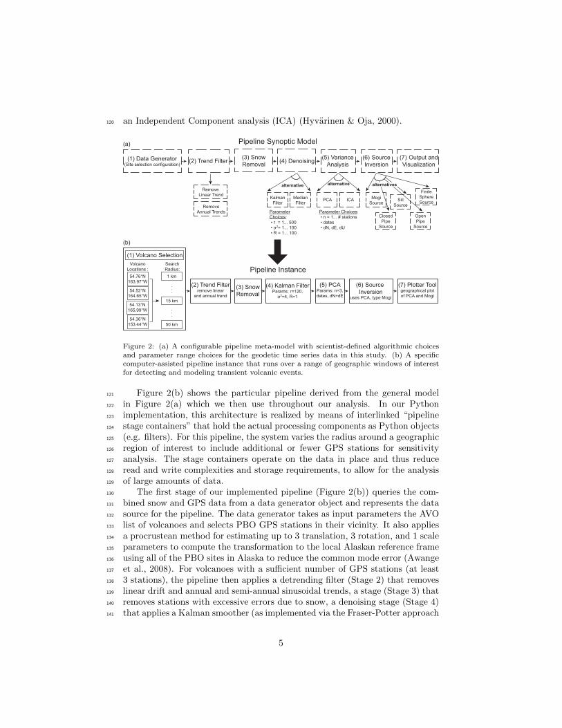
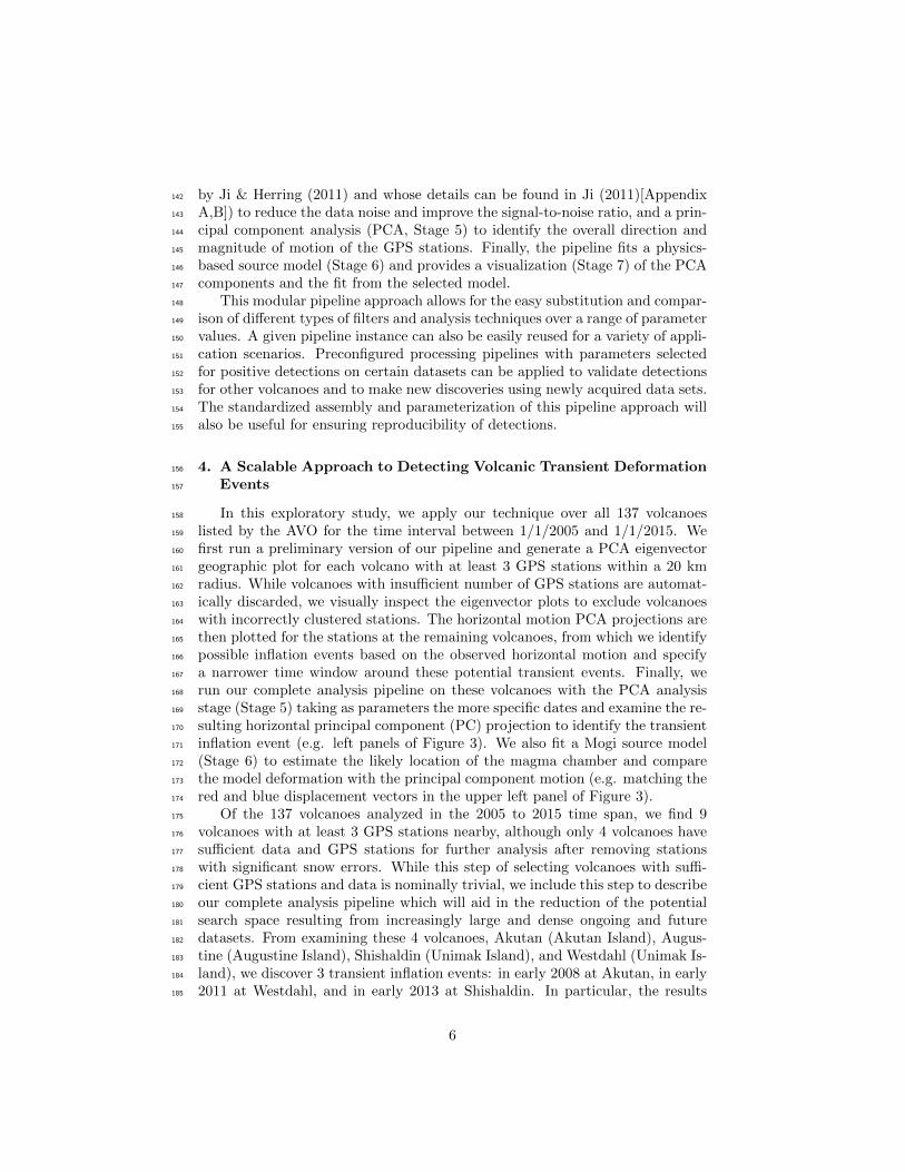

Jun
2012
Sep
201
2
Dec
201
2
Mar
201
3
Jun
2013
Sep
201
3
Dec
201
3
Mar
201
4
Jun
2014
Sep
201
4
Dec
201
4
Mar
201
5minus15
minus10
minus5
0
5
10
15
Am
plit
ud
e (
mm
)
Shishaldin First Horizontal Principal Component
(b)
(a)
minus10
minus5
0
5
10
15
Am
plit
ud
e (
mm
)
Westdahl First Horizontal Principal Component
Aug
200
9
Feb 2
010
Aug
201
0
Feb 2
011
Aug
201
1
Feb 2
012
Aug
201
2
Feb 2
0131649degW 1647degW 1645degW
544degN
545degN
546degN
547degN
Westdahl
AV25
AV26
15
km
AV24
Model Displacement
PCA Displacement
20
1642degW 164degW 1638degW
546degN
547degN
548degN
549degN
Shishaldin
AV37
AV39
20
Model Displacement
PCA Displacement
AV36
AV38
15km
Figure 5 Observations of newly detected transient inflation events (a) from early 2013 and toearly 2015 at Shishaldin volcano on Unimak Island Alaska and (b) from early 2011 to 2012at Westdahl volcano on Unimak Island Alaska Note that some of the spikes in the data arelikely artifacts due to snow Two additional GPS stations were available for Westdahl in thistime region but were not used due to large portions of the data being corrupted by snowThe 20 arrows in the plots indicate the scaling of the vectors relative to the respective firsthorizontal PCA componentrsquos amplitude
persisted until early 2015 the inflation event may also be connected with an248
effusive eruption in 2014 and with later reports of seismic and steam activity at249
Shishaldin that persisted through 2015 While the analysis of stations located250
on opposite sides of the volcanoes in Figure 4 shows a clear transient signal251
observed at Akutan and Shishaldin the signal at Westdahl is less clear This is252
likely due to the limitations of stations AV26 and AV24 at Westdahl not being253
located on directly opposite sides of the volcano resulting in a noisier difference254
52 Advantages of Configurable Computer-Aided Volcanic Data Processing Pipelines255
To our knowledge neither of these inflation events have been previously256
described in other works demonstrating the capability of our newly described257
10
computer aided discovery system for assisted rapid discovery This approach258
differs from previous work such as Ji amp Herring (2011) which considered the259
entire region of Alaska and observed the strong eigenvector motion only at260
Akutan Rather than attempting to detect an exceptionally strong signal out of261
the background noise which risks missing smaller events this pipeline approach262
targets known locations of interest and analyzes these regions at varying spatial263
scales This multiscale approach can be successively applied to larger geographic264
areas by specifying grids of interest and running the pipeline on time series265
obtained from the respective GPS stations Potentially this approach may266
also enable real-time or near real-time detection of future inflation events by267
continuous analysis of real-time GPS observations268
A particular output provided by our framework is a heatmap (Figure 6) that269
allows comparison of results from different pipeline configurations where each270
configuration makes different assumptions about underlying physics For our271
Akutan case we demonstrate here an example of this functionality by testing272
25 different configurations with implicitly different noise properties as addressed273
by Kalman smoothers with certain parameters or a median filter with varying274
window lengths The results in Figure 6 are compared using a color scheme that275
represents the difference between configurations as measured by the sum of all276
Euclidean distances between the eigenvectors obtained at each PBO station277
The colors in the heatmap in essence describe ldquohow differentrdquo pipeline results278
are given various assumptions The colors indicate groups of similar configura-279
tions which could help structure ideal configurations for further studies This280
output can reveal visual hints for potential alternative models that might fit281
the same empirical observations with different algorithmic choices and parame-282
ters In our particular numerical example for Akutan however the differences283
even between the maximum and minimum parameter values were minimal so284
we simply present the results from the initial configuration Configuration 00285
(The full list of configuration parameters can be found in the Appendix) This286
capability to vary configuration parameters extends to all stages of the pipeline287
including adjusting the details of the reference frame stabilization to remove288
common mode errors in the data generator stage (Stage 1 Figure 2)289
53 Fitting Magma Chamber Model Variants290
We combine the output from the PCA analysis with the smoothed detrended291
GPS position time series to determine station displacements which can be used292
in the model inversion analysis stage to fit a magma chamber source associated293
with the detected inflation event Using another set of configurations we can294
test different model variants to evaluate a best fit that describes the observed295
3-dimensional surface displacements as characterized with arctangent parame-296
terizations Here we fit the standard Mogi point source model (Mogi 1958) and297
then evaluate the effect of modeling the magma chamber at Akutan as a finite298
sphere a closed pipe a constant (width) open pipe or a sill-like magma source299
(Dzurisin 2006) The results of testing different magma source types is shown300
in Figure 7 The geographic plot in Figure 7(a) reveals that the source location301
is mostly stable across the different models As measured by the heatmap in302
11
Co
nfig
ura
tio
n 2
0C
on
fig
ura
tio
n 0
7C
on
fig
ura
tio
n 0
8C
on
fig
ura
tio
n 1
3C
on
fig
ura
tio
n 0
2C
on
fig
ura
tio
n 0
9C
on
fig
ura
tio
n 1
9C
on
fig
ura
tio
n 1
2C
on
fig
ura
tio
n 2
1C
on
fig
ura
tio
n 2
3C
on
fig
ura
tio
n 0
3C
on
fig
ura
tio
n 0
6C
on
fig
ura
tio
n 1
6C
on
fig
ura
tio
n 1
1C
on
fig
ura
tio
n 0
5C
on
fig
ura
tio
n 0
1C
on
fig
ura
tio
n 1
0C
on
fig
ura
tio
n 0
0C
on
fig
ura
tio
n 0
4C
on
fig
ura
tio
n 1
5C
on
fig
ura
tio
n 2
2C
on
fig
ura
tio
n 1
7C
on
fig
ura
tio
n 1
8C
on
fig
ura
tio
n 1
4C
on
fig
ura
tio
n 2
4
Configuration 24
Configuration 14
Configuration 18
Configuration 17
Configuration 22
Configuration 15
Configuration 04
Configuration 00
Configuration 10
Configuration 01
Configuration 05
Configuration 11
Configuration 16
Configuration 06
Configuration 03
Configuration 23
Configuration 21
Configuration 12
Configuration 19
Configuration 09
Configuration 02
Configuration 13
Configuration 08
Configuration 07
Configuration 20
000003006009012015
Similarity Metric
PCA Vector Distance
Figure 6 A heatmap showing the sum of the euclidean distance between the eigenvectorsat each PBO station for each sensitivity analysis run at Akutan Colors reflect the distancebetween results from different configurations as measured by the total difference between PCAeigenvectors at each PBO station Visualization of configurations provides natural groupingsof potential model assumptions for the given Akutan empirical data set The actual parametersfor each configuration are provided in the Appendix
Figure 7(b) only the sill-like magma source results in a less similar model and303
even then the difference is not substantial with at most a combined difference of304
around 3 mm between the projected displacement vectors at all PBO stations as305
compared with around 30 mm of total motion This minimal difference is also306
reflected by the mostly-negligible difference in projected displacement vectors307
shown in red in Figure 7(a) Further work could account for additional model308
types as well as more complex combinations of magma sources309
54 Instrument Sensor Network Requirements and Future Trends310
The four Alaskan volcanoes examined in this study Akutan Augustine311
Westdahl and Shishaldin have a sufficiently dense network of GPS receivers312
for running PCA but Westdahl demonstrates a greater detection uncertainty313
due to its less dense network of GPS stations The verification of the transient314
12
Sill
Const
ant
Open P
ipe
Clo
sed P
ipe
Mogi
Fin
ite S
phere
Finite Sphere
Mogi
Closed Pipe
Constant
Open Pipe
Sill
(a) (b)
000612182430
Similarity Metric
Summed Mogi
Vector Distance [mm]
20
AV07
AV08 AV14
AV10
AV06
AV15
AV12
1661
degW
166degW
1659
degW
1658
degW
1657
degW
54degN
541degN
542degN
543degN
Model Displacement
PCA Displacement
Figure 7 Comparison of 5 different source model inversions ndash Mogi finite sphere closedpipe constant (width) open pipe and sill ndash for the motion described by the eigenvectorsfor Akutan displayed on (a) a geographical plot with the eigenvectors in blue the differentinversion displacements in red (the solid color is the mean) and the different magma sourcelocations in green (the solid color shows the average location) The 20 arrow indicates thescaling of the vectors relative to the respective first horizontal PCA componentrsquos amplitude(b)A heatmap that compares the summed Euclidean distance [mm] between model displacementvectors at each GPS station for different model sources
event in Figure 4(c) is less distinct and the error ellipses in Figure 5(b) are315
larger than those in Figure 3 for Akutan and Figure 5(a) for Shishaldin This316
higher uncertainty in the case of Westdahl or the inability to conduct further317
analysis as in the case of other Alaskan volcanoes listed by the AVO is often due318
to the reduced number of available GPS stations after removing stations with319
corrupted data This data loss which results from the accumulation of snow320
and ice on the GPS antenna could be mitigated by using an improved filter321
that better corrects for the corrupted data or by more accurately removing only322
the corrupted sections of data instead of the current approach of rejecting the323
station entirely As an example in the case of Westdahl two additional GPS324
stations which were excluded from this study when examining the combined325
PBO and NSIDC data might become useable326
Consequently our approach is limited by the amount of available data at327
any given location requiring volcanoes or other points of interest to be in-328
strumented with a sufficiently dense network of sensors However this work329
looks forward towards the decreasing cost of sensors and the trend of increasing330
density of GPS stations and the resulting increase in volume of data As larger331
and higher resolution sensor networks are deployed across the entire planet tra-332
ditionally manual approaches become inefficient making Big Data analysis a333
13
key bottleneck in the scientific discovery process This work demonstrates that334
our approach can enable scientists to study more difficult problems by better335
utilizing large amounts of data336
A key capability of an automated assisted system is the ability to aid in337
downloading parsing and analyzing increasingly large data sets Given a broad338
range of scientific applications using GPS data we downloaded the data set for339
all PBO GPS stations (sim1GB) From that larger data set when we focus on340
exploring events associated with volcanic activity our pipeline automatically341
narrows down the relevant GPS stations based on the provided coordinates of342
interest Furthermore as different types of instruments cover the same geo-343
graphical region of interest this pipeline framework also helps integrate addi-344
tional sources of data Here the pipeline preprocesses and integrates the snow345
cover NSIDC data (an additional 150 GB data set) And as more GPS stations346
are established and additional data sources such as InSAR are integrated into347
a cohesive analysis the computational footprint for data analysis will continue348
to increase349
The flexibility of our framework allows it to be adapted to data sets as350
they become available Although the transient inflation events discussed here351
have been on the order of months to years with higher time resolution data of352
the same precision shorter events could also be detected Furthermore while353
the motion that characterizes transient events only becomes detectable after a354
period of time real-time or near real-time monitoring can be implemented to355
aid in providing early warning of volcanic activity356
6 Conclusion357
This article introduces a computer-aided discovery approach that develops358
a framework for studying transient events at volcanoes using configurable data359
processing pipelines We demonstrate its applicability and utility by detecting360
and analyzing transient inflation events at 3 Alaskan volcanoes Akutan on Aku-361
tan Island and Westdahl and Shishaldin on Unimak Island Our results include362
the discovery of two inflation events that have not been previously reported in363
the literature364
The study of transient events at Alaskan volcanoes exemplifies how volcanic365
data exploration can be a considerable challenge for scientists due to the large366
search space of potential events and event features hidden within large amounts367
of data Computer assistance and automation expedites the analysis of multi-368
scale transient deformation events at a large number of sites of interest our369
system is assembled from easily reusable modular analysis stages providing an370
extensible structure that can be used to explore multiple deformation hypothe-371
ses efficiently In the future we envision that such techniques will become a key372
component in processing the data collected from ever growing sensor networks373
that produce increasingly large amounts of data In addition these computa-374
tional pipelines can be expanded to take advantage of data fusion from other375
data sources such as InSAR to aid in the detection and analysis of earth surface376
deformation and volcanic events377
14
While our overall computer-aided discovery framework is still under con-378
tinued revision and development we have released our Python package for ac-379
cessing various scientific datasets online as the SciKit Data Access (skdaccess)380
package This package can be easily installed through the Python Package In-381
dex (httpspypipythonorgpypiskdaccess) and the source code is available382
on GitHub (httpsgithubcomskdaccessskdaccess) We plan to release the383
analysis package incrementally in a similar fashion To promote the importance384
of open code and open science usage of our framework and code will be covered385
under the MIT Open License386
Acknowledgements387
We acknowledge support from NASA AIST NNX15AG84G NSF ACI 1442997388
and the Amazon Web Services Research Grant This material is based on Earth-389
Scope Plate Boundary Observatory data services provided by UNAVCO through390
the GAGE Facility with support from the National Science Foundation (NSF)391
and National Aeronautics and Space Administration (NASA) under NSF Co-392
operative Agreement No EAR-1261833393
References394
Alaska Volcano Observatory Akutan Westdahl and Shishaldin Reported Ac-395
tivity last accessed 512016 URL httpswwwavoalaskaedu396
Amazon Web Services (2015) Overview of Amazon Web Services (white paper)397
Awange J L Bae K H amp Claessens S J (2008) Procrustean solution of the398
9-parameter transformation problem Earth Planets and Space 60 529ndash537399
URL httpdxdoiorg101186BF03353115 doi101186BF03353115400
Czarnecki K amp Eisenecker U W (2000) Generative Programming Methods401
Tools and Applications Addison-Wesley402
Dong D Fang P Bock Y Webb F Prawirodirdjo L Kedar S amp403
Jamason P (2006) Spatiotemporal filtering using principal component404
analysis and Karhunen-Loeve expansion approaches for regional GPS net-405
work analysis Journal of Geophysical Research Solid Earth 111 URL406
httpdxdoiorg1010292005JB003806 doi1010292005JB003806407
Dzurisin D (2006) Volcano deformation new geodetic monitoring techniques408
Springer Science amp Business Media409
Gong W Meyer F J Lee C-W Lu Z amp Freymueller J (2015) Mea-410
surement and interpretation of subtle deformation signals at Unimak Island411
from 2003 to 2010 using weather model-assisted time series InSAR Jour-412
nal of Geophysical Research Solid Earth 120 1175ndash1194 URL http413
dxdoiorg1010022014JB011384 doi1010022014JB011384414
15
Hyvarinen A amp Oja E (2000) Independent component analysis al-415
gorithms and applications Neural Networks 13 411ndash430 URL http416
wwwsciencedirectcomsciencearticlepiiS0893608000000265417
doihttpdxdoiorg101016S0893-6080(00)00026-5418
Ji K H (2011) Transient signal detection using GPS position time series419
PhD thesis Massachusetts Institute of Technology420
Ji K H amp Herring T A (2011) Transient signal detection using GPS mea-421
surements Transient inflation at Akutan volcano Alaska during early 2008422
Geophysical Research Letters 38 doi1010292011GL046904423
Kositsky A P amp Avouac J-P (2010) Inverting geodetic time series with424
a principal component analysis-based inversion method Journal of Geo-425
physical Research Solid Earth 115 URL httpdxdoiorg101029426
2009JB006535 doi1010292009JB006535427
Langbein J (2008) Noise in GPS displacement measurements from Southern428
California and Southern Nevada Journal of Geophysical Research Solid429
Earth 113 URL httpdxdoiorg1010292007JB005247 doi10430
10292007JB005247431
Lin Y-n N Kositsky A P amp Avouac J-P (2010) PCAIM joint inver-432
sion of InSAR and ground-based geodetic time series Application to mon-433
itoring magmatic inflation beneath the Long Valley Caldera Geophysical434
Research Letters 37 URL httpdxdoiorg1010292010GL045769435
doi1010292010GL045769436
Lu Z Masterlark T Dzurisin D Rykhus R amp Wicks C (2003) Magma437
supply dynamics at Westdahl volcano Alaska modeled from satellite radar438
interferometry Journal of Geophysical Research Solid Earth 108 URL439
httpdxdoiorg1010292002JB002311 doi1010292002JB002311440
Mann D amp Freymueller J (2003) Volcanic and tectonic deforma-441
tion on Unimak Island in the Aleutian Arc Alaska Journal of Geo-442
physical Research Solid Earth 108 URL httpdxdoiorg101029443
2002JB001925 doi1010292002JB001925444
Mogi K (1958) Relations between the eruptions of vari-445
ous volcanoes and the deformations of the ground surfaces446
around them URL httprepositorydlitcu-tokyoac447
jpdspacehandle226111909$delimiter026E30F$npapers448
8461d6ef-4184-45b2-aa3d-395291ea6525Paperp3868 doi101016449
jepsl200404016450
National Ice Center (2008) IMS Daily Northern Hemisphere Snow and Ice451
Analysis at 1 km 4 km and 24 km Resolutions Version 1 URL http452
dxdoiorg107265N52R3PMC453
16
Pankratius V Li J Gowanlock M Blair D M Rude C Herring T Lind454
F Erickson P J amp Lonsdale C (JulyAugust 2016) Computer-Aided Dis-455
covery Towards Scientific Insight Generation with Machine Support IEEE456
Intelligent Systems 37(4) 3ndash10457
Appendix458
The heatmap in Figure 6 is generated from multiple executions of the pipeline459
using the configurations listed below where the filteringsmoothing stage was460
perturbed For the Kalman filter stage container the three parameters are τ461
(correlation time in days) σ2 (variance of the correlated noise) and R (mea-462
surement noise) For the median filter the one parameter is the window length463
(the number of days of the window for calculating the median) To give two464
examples from our 25 configurations Configuration 0 employs a Kalman filter465
with a τ of 120 a σ2 of 4 and an R of 1 and Configuration 2 employs a median466
filter with a window length of 79 days467
468
Configuration 0 KalmanFilter1[rsquo120rsquo rsquo4rsquo rsquo1rsquo]469
Configuration 1 KalmanFilter1[rsquo65rsquo rsquo99rsquo rsquo65rsquo]470
Configuration 2 MedianFilter[rsquo79rsquo]471
Configuration 3 MedianFilter[rsquo23rsquo]472
Configuration 4 KalmanFilter1[rsquo191rsquo rsquo46rsquo rsquo8rsquo]473
Configuration 5 KalmanFilter1[rsquo417rsquo rsquo19rsquo rsquo86rsquo]474
Configuration 6 MedianFilter[rsquo34rsquo]475
Configuration 7 MedianFilter[rsquo51rsquo]476
Configuration 8 MedianFilter[rsquo98rsquo]477
Configuration 9 MedianFilter[rsquo70rsquo]478
Configuration 10 KalmanFilter1[rsquo279rsquo rsquo76rsquo rsquo11rsquo]479
Configuration 11 KalmanFilter1[rsquo500rsquo rsquo100rsquo rsquo1rsquo]480
Configuration 12 MedianFilter[rsquo88rsquo]481
Configuration 13 MedianFilter[rsquo69rsquo]482
Configuration 14 KalmanFilter1[rsquo241rsquo rsquo86rsquo rsquo89rsquo]483
Configuration 15 KalmanFilter1[rsquo500rsquo rsquo51rsquo rsquo96rsquo]484
Configuration 16 MedianFilter[rsquo32rsquo]485
Configuration 17 KalmanFilter1[rsquo421rsquo rsquo48rsquo rsquo56rsquo]486
Configuration 18 KalmanFilter1[rsquo60rsquo rsquo5rsquo rsquo30rsquo]487
Configuration 19 MedianFilter[rsquo75rsquo]488
Configuration 20 KalmanFilter1[rsquo500rsquo rsquo1rsquo rsquo100rsquo]489
Configuration 21 MedianFilter[rsquo87rsquo]490
Configuration 22 KalmanFilter1[rsquo207rsquo rsquo26rsquo rsquo95rsquo]491
Configuration 23 MedianFilter[rsquo83rsquo]492
Configuration 24 KalmanFilter1[rsquo225rsquo rsquo52rsquo rsquo34rsquo]493
17
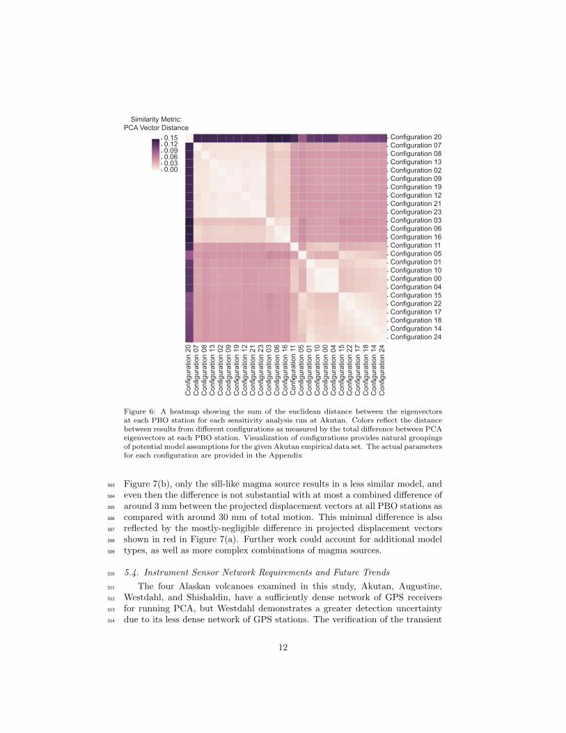

Sill
Const
ant
Open P
ipe
Clo
sed P
ipe
Mogi
Fin
ite S
phere
Finite Sphere
Mogi
Closed Pipe
Constant
Open Pipe
Sill
(a) (b)
000612182430
Similarity Metric
Summed Mogi
Vector Distance [mm]
20
AV07
AV08 AV14
AV10
AV06
AV15
AV12
1661
degW
166degW
1659
degW
1658
degW
1657
degW
54degN
541degN
542degN
543degN
Model Displacement
PCA Displacement
Figure 7 Comparison of 5 different source model inversions ndash Mogi finite sphere closedpipe constant (width) open pipe and sill ndash for the motion described by the eigenvectorsfor Akutan displayed on (a) a geographical plot with the eigenvectors in blue the differentinversion displacements in red (the solid color is the mean) and the different magma sourcelocations in green (the solid color shows the average location) The 20 arrow indicates thescaling of the vectors relative to the respective first horizontal PCA componentrsquos amplitude(b)A heatmap that compares the summed Euclidean distance [mm] between model displacementvectors at each GPS station for different model sources
event in Figure 4(c) is less distinct and the error ellipses in Figure 5(b) are315
larger than those in Figure 3 for Akutan and Figure 5(a) for Shishaldin This316
higher uncertainty in the case of Westdahl or the inability to conduct further317
analysis as in the case of other Alaskan volcanoes listed by the AVO is often due318
to the reduced number of available GPS stations after removing stations with319
corrupted data This data loss which results from the accumulation of snow320
and ice on the GPS antenna could be mitigated by using an improved filter321
that better corrects for the corrupted data or by more accurately removing only322
the corrupted sections of data instead of the current approach of rejecting the323
station entirely As an example in the case of Westdahl two additional GPS324
stations which were excluded from this study when examining the combined325
PBO and NSIDC data might become useable326
Consequently our approach is limited by the amount of available data at327
any given location requiring volcanoes or other points of interest to be in-328
strumented with a sufficiently dense network of sensors However this work329
looks forward towards the decreasing cost of sensors and the trend of increasing330
density of GPS stations and the resulting increase in volume of data As larger331
and higher resolution sensor networks are deployed across the entire planet tra-332
ditionally manual approaches become inefficient making Big Data analysis a333
13
key bottleneck in the scientific discovery process This work demonstrates that334
our approach can enable scientists to study more difficult problems by better335
utilizing large amounts of data336
A key capability of an automated assisted system is the ability to aid in337
downloading parsing and analyzing increasingly large data sets Given a broad338
range of scientific applications using GPS data we downloaded the data set for339
all PBO GPS stations (sim1GB) From that larger data set when we focus on340
exploring events associated with volcanic activity our pipeline automatically341
narrows down the relevant GPS stations based on the provided coordinates of342
interest Furthermore as different types of instruments cover the same geo-343
graphical region of interest this pipeline framework also helps integrate addi-344
tional sources of data Here the pipeline preprocesses and integrates the snow345
cover NSIDC data (an additional 150 GB data set) And as more GPS stations346
are established and additional data sources such as InSAR are integrated into347
a cohesive analysis the computational footprint for data analysis will continue348
to increase349
The flexibility of our framework allows it to be adapted to data sets as350
they become available Although the transient inflation events discussed here351
have been on the order of months to years with higher time resolution data of352
the same precision shorter events could also be detected Furthermore while353
the motion that characterizes transient events only becomes detectable after a354
period of time real-time or near real-time monitoring can be implemented to355
aid in providing early warning of volcanic activity356
6 Conclusion357
This article introduces a computer-aided discovery approach that develops358
a framework for studying transient events at volcanoes using configurable data359
processing pipelines We demonstrate its applicability and utility by detecting360
and analyzing transient inflation events at 3 Alaskan volcanoes Akutan on Aku-361
tan Island and Westdahl and Shishaldin on Unimak Island Our results include362
the discovery of two inflation events that have not been previously reported in363
the literature364
The study of transient events at Alaskan volcanoes exemplifies how volcanic365
data exploration can be a considerable challenge for scientists due to the large366
search space of potential events and event features hidden within large amounts367
of data Computer assistance and automation expedites the analysis of multi-368
scale transient deformation events at a large number of sites of interest our369
system is assembled from easily reusable modular analysis stages providing an370
extensible structure that can be used to explore multiple deformation hypothe-371
ses efficiently In the future we envision that such techniques will become a key372
component in processing the data collected from ever growing sensor networks373
that produce increasingly large amounts of data In addition these computa-374
tional pipelines can be expanded to take advantage of data fusion from other375
data sources such as InSAR to aid in the detection and analysis of earth surface376
deformation and volcanic events377
14
While our overall computer-aided discovery framework is still under con-378
tinued revision and development we have released our Python package for ac-379
cessing various scientific datasets online as the SciKit Data Access (skdaccess)380
package This package can be easily installed through the Python Package In-381
dex (httpspypipythonorgpypiskdaccess) and the source code is available382
on GitHub (httpsgithubcomskdaccessskdaccess) We plan to release the383
analysis package incrementally in a similar fashion To promote the importance384
of open code and open science usage of our framework and code will be covered385
under the MIT Open License386
Acknowledgements387
We acknowledge support from NASA AIST NNX15AG84G NSF ACI 1442997388
and the Amazon Web Services Research Grant This material is based on Earth-389
Scope Plate Boundary Observatory data services provided by UNAVCO through390
the GAGE Facility with support from the National Science Foundation (NSF)391
and National Aeronautics and Space Administration (NASA) under NSF Co-392
operative Agreement No EAR-1261833393
References394
Alaska Volcano Observatory Akutan Westdahl and Shishaldin Reported Ac-395
tivity last accessed 512016 URL httpswwwavoalaskaedu396
Amazon Web Services (2015) Overview of Amazon Web Services (white paper)397
Awange J L Bae K H amp Claessens S J (2008) Procrustean solution of the398
9-parameter transformation problem Earth Planets and Space 60 529ndash537399
URL httpdxdoiorg101186BF03353115 doi101186BF03353115400
Czarnecki K amp Eisenecker U W (2000) Generative Programming Methods401
Tools and Applications Addison-Wesley402
Dong D Fang P Bock Y Webb F Prawirodirdjo L Kedar S amp403
Jamason P (2006) Spatiotemporal filtering using principal component404
analysis and Karhunen-Loeve expansion approaches for regional GPS net-405
work analysis Journal of Geophysical Research Solid Earth 111 URL406
httpdxdoiorg1010292005JB003806 doi1010292005JB003806407
Dzurisin D (2006) Volcano deformation new geodetic monitoring techniques408
Springer Science amp Business Media409
Gong W Meyer F J Lee C-W Lu Z amp Freymueller J (2015) Mea-410
surement and interpretation of subtle deformation signals at Unimak Island411
from 2003 to 2010 using weather model-assisted time series InSAR Jour-412
nal of Geophysical Research Solid Earth 120 1175ndash1194 URL http413
dxdoiorg1010022014JB011384 doi1010022014JB011384414
15
Hyvarinen A amp Oja E (2000) Independent component analysis al-415
gorithms and applications Neural Networks 13 411ndash430 URL http416
wwwsciencedirectcomsciencearticlepiiS0893608000000265417
doihttpdxdoiorg101016S0893-6080(00)00026-5418
Ji K H (2011) Transient signal detection using GPS position time series419
PhD thesis Massachusetts Institute of Technology420
Ji K H amp Herring T A (2011) Transient signal detection using GPS mea-421
surements Transient inflation at Akutan volcano Alaska during early 2008422
Geophysical Research Letters 38 doi1010292011GL046904423
Kositsky A P amp Avouac J-P (2010) Inverting geodetic time series with424
a principal component analysis-based inversion method Journal of Geo-425
physical Research Solid Earth 115 URL httpdxdoiorg101029426
2009JB006535 doi1010292009JB006535427
Langbein J (2008) Noise in GPS displacement measurements from Southern428
California and Southern Nevada Journal of Geophysical Research Solid429
Earth 113 URL httpdxdoiorg1010292007JB005247 doi10430
10292007JB005247431
Lin Y-n N Kositsky A P amp Avouac J-P (2010) PCAIM joint inver-432
sion of InSAR and ground-based geodetic time series Application to mon-433
itoring magmatic inflation beneath the Long Valley Caldera Geophysical434
Research Letters 37 URL httpdxdoiorg1010292010GL045769435
doi1010292010GL045769436
Lu Z Masterlark T Dzurisin D Rykhus R amp Wicks C (2003) Magma437
supply dynamics at Westdahl volcano Alaska modeled from satellite radar438
interferometry Journal of Geophysical Research Solid Earth 108 URL439
httpdxdoiorg1010292002JB002311 doi1010292002JB002311440
Mann D amp Freymueller J (2003) Volcanic and tectonic deforma-441
tion on Unimak Island in the Aleutian Arc Alaska Journal of Geo-442
physical Research Solid Earth 108 URL httpdxdoiorg101029443
2002JB001925 doi1010292002JB001925444
Mogi K (1958) Relations between the eruptions of vari-445
ous volcanoes and the deformations of the ground surfaces446
around them URL httprepositorydlitcu-tokyoac447
jpdspacehandle226111909$delimiter026E30F$npapers448
8461d6ef-4184-45b2-aa3d-395291ea6525Paperp3868 doi101016449
jepsl200404016450
National Ice Center (2008) IMS Daily Northern Hemisphere Snow and Ice451
Analysis at 1 km 4 km and 24 km Resolutions Version 1 URL http452
dxdoiorg107265N52R3PMC453
16
Pankratius V Li J Gowanlock M Blair D M Rude C Herring T Lind454
F Erickson P J amp Lonsdale C (JulyAugust 2016) Computer-Aided Dis-455
covery Towards Scientific Insight Generation with Machine Support IEEE456
Intelligent Systems 37(4) 3ndash10457
Appendix458
The heatmap in Figure 6 is generated from multiple executions of the pipeline459
using the configurations listed below where the filteringsmoothing stage was460
perturbed For the Kalman filter stage container the three parameters are τ461
(correlation time in days) σ2 (variance of the correlated noise) and R (mea-462
surement noise) For the median filter the one parameter is the window length463
(the number of days of the window for calculating the median) To give two464
examples from our 25 configurations Configuration 0 employs a Kalman filter465
with a τ of 120 a σ2 of 4 and an R of 1 and Configuration 2 employs a median466
filter with a window length of 79 days467
468
Configuration 0 KalmanFilter1[rsquo120rsquo rsquo4rsquo rsquo1rsquo]469
Configuration 1 KalmanFilter1[rsquo65rsquo rsquo99rsquo rsquo65rsquo]470
Configuration 2 MedianFilter[rsquo79rsquo]471
Configuration 3 MedianFilter[rsquo23rsquo]472
Configuration 4 KalmanFilter1[rsquo191rsquo rsquo46rsquo rsquo8rsquo]473
Configuration 5 KalmanFilter1[rsquo417rsquo rsquo19rsquo rsquo86rsquo]474
Configuration 6 MedianFilter[rsquo34rsquo]475
Configuration 7 MedianFilter[rsquo51rsquo]476
Configuration 8 MedianFilter[rsquo98rsquo]477
Configuration 9 MedianFilter[rsquo70rsquo]478
Configuration 10 KalmanFilter1[rsquo279rsquo rsquo76rsquo rsquo11rsquo]479
Configuration 11 KalmanFilter1[rsquo500rsquo rsquo100rsquo rsquo1rsquo]480
Configuration 12 MedianFilter[rsquo88rsquo]481
Configuration 13 MedianFilter[rsquo69rsquo]482
Configuration 14 KalmanFilter1[rsquo241rsquo rsquo86rsquo rsquo89rsquo]483
Configuration 15 KalmanFilter1[rsquo500rsquo rsquo51rsquo rsquo96rsquo]484
Configuration 16 MedianFilter[rsquo32rsquo]485
Configuration 17 KalmanFilter1[rsquo421rsquo rsquo48rsquo rsquo56rsquo]486
Configuration 18 KalmanFilter1[rsquo60rsquo rsquo5rsquo rsquo30rsquo]487
Configuration 19 MedianFilter[rsquo75rsquo]488
Configuration 20 KalmanFilter1[rsquo500rsquo rsquo1rsquo rsquo100rsquo]489
Configuration 21 MedianFilter[rsquo87rsquo]490
Configuration 22 KalmanFilter1[rsquo207rsquo rsquo26rsquo rsquo95rsquo]491
Configuration 23 MedianFilter[rsquo83rsquo]492
Configuration 24 KalmanFilter1[rsquo225rsquo rsquo52rsquo rsquo34rsquo]493
17
Recommended