Consistency of heterogeneous synchronization patterns in complex weighted networksD. Malagarriga, A. E. P. Villa, J. Garcia-Ojalvo, and A. J. Pons
Citation: Chaos 27, 031102 (2017); doi: 10.1063/1.4977972View online: http://dx.doi.org/10.1063/1.4977972View Table of Contents: http://aip.scitation.org/toc/cha/27/3Published by the American Institute of Physics
Articles you may be interested inAre continuum predictions of clustering chaotic?Chaos 27, 031101031101 (2017); 10.1063/1.4977513
Modeling the network dynamics of pulse-coupled neuronsChaos 27, 033102033102 (2017); 10.1063/1.4977514
Extremes in dynamic-stochastic systemsChaos 27, 012101012101 (2017); 10.1063/1.4973541
Nonlinear resonances and multi-stability in simple neural circuitsChaos 27, 013118013118 (2017); 10.1063/1.4974028
Levitation of heavy particles against gravity in asymptotically downward flowsChaos 27, 031103031103 (2017); 10.1063/1.4978386
Chaotic oscillator containing memcapacitor and meminductor and its dimensionality reduction analysisChaos 27, 033103033103 (2017); 10.1063/1.4975825
Consistency of heterogeneous synchronization patterns in complexweighted networks
D. Malagarriga,1,2,a) A. E. P. Villa,3 J. Garcia-Ojalvo,4 and A. J. Pons1
1Departament de F�ısica, Universitat Politecnica de Catalunya. Edifici Gaia, Rambla Sant Nebridi 22,08222 Terrassa, Spain2Centre for Genomic Regulation (CRG). Barcelona Biomedical Research Park (PRBB), Dr. Aiguader 88,08003 Barcelona, Spain3Neuroheuristic Research Group, Faculty of Business and Economics, University of Lausanne.CH-1015 Lausanne, Switzerland4Department of Experimental and Health Sciences, Universitat Pompeu Fabra, Barcelona BiomedicalResearch Park (PRBB), Dr. Aiguader 88, 08003 Barcelona, Spain
(Received 22 January 2017; accepted 20 February 2017; published online 9 March 2017)
Synchronization within the dynamical nodes of a complex network is usually considered
homogeneous through all the nodes. Here we show, in contrast, that subsets of interacting oscillators
may synchronize in different ways within a single network. This diversity of synchronization patterns
is promoted by increasing the heterogeneous distribution of coupling weights and/or asymmetries in
small networks. We also analyze consistency, defined as the persistence of coexistent synchronization
patterns regardless of the initial conditions. Our results show that complex weighted networks display
richer consistency than regular networks, suggesting why certain functional network topologies
are often constructed when experimental data are analyzed. VC 2017 Author(s). All article content,except where otherwise noted, is licensed under a Creative Commons Attribution (CC BY) license(http://creativecommons.org/licenses/by/4.0/). [http://dx.doi.org/10.1063/1.4977972]
Dynamical systems may synchronize in several ways, at
the same time, when they are coupled in a single complex
network. Examples of this diversity of synchronization
patterns may be found in research fields as diverse as
neuroscience, climate networks, or ecosystems. Here we
report the conditions required to obtain coexisting syn-
chronizations in arrangements of interacting chaotic
oscillators, and relate these conditions to the distribution
of coupling weights and asymmetries in complex net-
works. We also analyze the conditions required for a high
statistical occurrence of the same synchronization pat-
terns, regardless of the oscillators’ initial conditions. Our
results show that these persistent synchronization pat-
terns are statistically more frequent in complex weighted
networks than in regular ones, explaining why certain
functional network topologies are often retrieved from
experimental data. Besides, our results suggest that con-
sidering both the different coexisting synchronizations
and also their statistics may result in a richer under-
standing of the relations between functional and struc-
tural networks of oscillators.
I. INTRODUCTION
Certain dynamical systems, which display oscillatory
behavior in isolation, may display a wide repertoire of
dynamical evolutions due to the coupling with their neigh-
bors when embedded in networks of similar complex items.1
The relationship between network dynamics and structure in
this type of systems is therefore a fundamental question in
network science. For instance, the interaction of rhythmic
elements may entail an adjustment of their oscillatory
dynamics to finally end up in a state of (dynamical) agree-ment or synchronization.2–4 When coupling is strong, the
oscillators in a network usually synchronize in a particular
collective oscillatory behavior. However, for more moderate
coupling intensity, this relationship may also be inhomoge-
neous, i.e., certain oscillators may synchronize whereas
others may not.5–10 The specific patterns of synchronization,
thus, provide information about the underlying couplings
between the dynamical elements forming the network.
Hence, a better characterization of the system can be
achieved by analyzing all the synchronization relationships
within a network instead of analyzing a single synchroniza-
tion relationship. This type of characterization might be of
crucial importance when the details of the contacts between
the oscillators are not available.
In the past, studies of the synchronization patterns in
networks of oscillators were mainly aimed at describing the
conditions associated with the emergence of specific syn-
chronization patterns in all the nodes.11 In the particular case
of complex networks of coupled nonlinear oscillators, recent
studies have provided evidence that it is possible to identify
an appropriate interaction regime that allows to collect mea-
sured data to infer the underlying network structure based on
time-series statistical similarity analysis12 or connectivity
stability analysis.13 In real-life systems, such as ecological
networks,14 brain oscillations,15–18 or climate interactions,19
various types of complex synchronized dynamics have been
observed to coexist in a single network. Therefore, such a
diversity in dynamical relationships between the nodes
a)Author to whom correspondence should be addressed. Electronic mail:
1054-1500/2017/27(3)/031102/9 VC Author(s) 2017.27, 031102-1
CHAOS 27, 031102 (2017)
endows a network with stability, flexibility, and robustness
against perturbations.20
The present work reveals that several types of stable
synchronization patterns may coexist depending on the
topology and on the distribution of coupling strengths within
a network. Besides, the capacity of a network to display the
same heterogeneous synchronization pattern regardless of
the initial conditions, or consistency, is also investigated.
Such a property, observed in some type of networks, allows
to retrieve network structure from its dynamics in a more
reliable way than using single synchronization patterns.
II. COEXISTENCE OF SYNCHRONIZATIONS
Consider two n-dimensional dynamical systems, x and y,
whose temporal evolutions are generally defined by _xðtÞ ¼FðxðtÞÞ; _yðtÞ ¼ GðyðtÞÞ in isolation. Assuming a bidirectional
coupling scheme, the coupled system reads:
_xðtÞ ¼ FðxðtÞÞ þ CðyðtÞ � xðtÞÞ;_yðtÞ ¼ GðyðtÞÞ þ CðxðtÞ � yðtÞÞ: (1)
Here, x(t) and y(t) are the n-dimensional state vectors of the
systems, F and G are their corresponding vector fields, and C
is a n� n matrix that provides the coupling characteristics
between the sub-systems. When coupling is strong enough and
these dynamical systems are oscillators, the synchronization
relationships that can be established between them can be cate-
gorized in four types (see time traces in Fig. 1):22,23
• Phase synchronization (PS) appears if the functional rela-
tionship between the dynamics of two oscillators preserves
a bounded phase difference,24 with their amplitudes being
largely uncorrelated. This can be exemplified by the rela-
tionship jn/1 � m/2j < const, with n and m being integer
numbers which define the ratio between the phases /1;2 of
the two coupled oscillators.• Generalized synchronization (GS) is observed if a com-
plex functional relationship is established between the
oscillators,25 e.g., y(t)¼H[x(t)], where H[x(t)] can take
any form other than identity. It can be thought to be a gen-
eralization of complete synchronization (CS) for non-
identical oscillators.• Lag synchronization (LS) appears when the amplitude cor-
relation is high while at the same time there is a time shift
in the dynamics of the oscillators,26 y(t)¼ x(t – s), with sbeing a lag time.
• Complete synchronization (CS) is observed when the cou-
pled oscillators are identical or almost identical,27 and
x(t)¼ y(t) for a sufficiently large coupling strength C.
There are several analysis techniques that can be used to
assess the emergence of each of the mentioned synchronization
motifs. Here, three of them are combined: cross-correlation
(CC), Phase-Locking Value (PLV), and the Nearest-Neighbor
Method (NNM). CC computes the lagged similarity or sliding
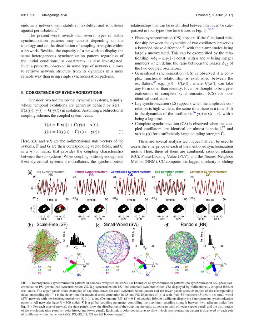
FIG. 1. Heterogeneous synchronization patterns in complex weighted networks. (a) Examples of synchronization patterns (no synchronization NS, phase syn-
chronization PS, generalized synchronization GS, lag synchronization LS, and complete synchronization CS) displayed by bidirectionally coupled R€ossler
oscillators. The upper panels show examples of xi(t) time traces for each synchronization pattern and the lower panels show examples of the corresponding
delay-embedding plot.21 s is the delay time for maximal cross-correlation in LS and PS. Examples of (b) a scale-free (SF) network (K¼ 0.4), (c) small-world
(SW) network with low rewiring probability (K¼ 0.1), and (D) random (RN) (K¼ 0.1) of coupled R€ossler oscillators displaying heterogeneous synchronization
patterns. All networks have N¼ 100 nodes. K is a global coupling parameter controlling the maximum coupling strength between two adjacent nodes (see
Eq. (3)). For each type of network the right panels show the distribution of the coupling strengths aij between pairs of nodes (upper panel) and the distribution
of the synchronization patterns (polar histogram, lower panel). Each link is color-coded so as to show which synchronization pattern is displayed by each pair
of oscillators within the network (NS, PS, GS, LS, CS see left bottom legend).
031102-2 Malagarriga et al. Chaos 27, 031102 (2017)
dot product between two signals, which provides a notion of
the amplitude resemblance over time. Therefore, it allows to
identify whether CS or LS is established between two time
traces. On the other hand, PLV makes use of the Hilbert trans-
form of a signal to retrieve a phase / and compute the time
evolution of the difference in the phases of two oscillators, i.e.,
/1ðtÞ � /2ðtÞ,28 as
PLVt ¼1
N
����XN
n¼1
heiD/12 t;nð Þit����; (2)
where D/12ðt; nÞ is the evolution of the difference between
the phases of oscillators 1 and 2, N is the number of trials,
and h…it denotes temporal average. This measure can
assess, when combined with low CC, the emergence of PS
between two oscillators. Finally, the NNM takes points in
the phase space of each oscillator and characterizes their rel-
ative evolution.27 This method allows to visualize and exem-
plify each synchronization motif as well as to identify the
emergence of generalized synchronization between two
oscillators21 (see examples in Fig. 1(a), lower panels). In
order to establish thresholds for each synchronized state we
computed an average distance d of the images uk;kn of the
nearest neighbors xk;kn of two coupled oscillators as per-
formed in Ref. 21. We took the reported values of d that indi-
cate the onset of each synchronization and compared these
values with our CC and PLV calculations in the same situa-
tion. Thanks to this, we established thresholds ni for comput-
ing each synchronization pattern in the particular case of
R€ossler oscillators: PS entails nPLV� 0.9 and nCC� 0.5 with
lag 0, GS can be identified if nPLV� 0.9 and nCC� 0.9
with lag� 1, LS is present if nPLV� 0.9 and nCC� 0.9
with 0� lag< 1, and finally CS emerges if nPLV� 0.9 and
nCC� 0.9 with lag¼ 0. With this set of analysis techniques,
here, the dynamics of networks of coupled R€ossler oscilla-
tors29 arranged in complex weighted topologies—random
(RN),30 small-world (SW),31 and scale-free (SF)32—are
studied.
The dynamics of each node i follow the 3-dimensional
R€ossler equations, which read
_xi ¼ �xiyi � zi þ KXNneigh
j¼1; j6¼i
aijðxj � xiÞ;
_yi ¼ xixi þ ayi;
_zi ¼ pþ ziðxi � cÞ; (3)
where K is a global parameter controlling the maximum cou-
pling strength between two nodes and xi is the natural fre-
quency of the node i, which is normally distributed with
average hxi ¼ 1 and standard deviation rx¼ 0.02. An isolated
node with R€ossler dynamics can display periodic, quasi-
periodic, or chaotic dynamics, and we choose a¼ 0.15,
p¼ 0.2, and c¼ 10 to set the oscillators into a chaotic regime.27
The coupling weights are set to depend on the number of
neighbors of each node, if not specified otherwise, as
aij ¼1ffiffiffiffiffiffiffiffiffiffiffiffiffiffiffiffiffiffiffiffiffiffiffiffiffiffiffiffi
deg við Þdeg vjð Þp ; (4)
for i 6¼ j, where deg(vi), deg(vj) are the degrees (number of
coupled neighbors) of two coupled nodes vi, vj.
Figures 1(b)–1(d) show the distribution of synchroniza-
tions in three prototypical networks (composed of N¼ 100
nodes), namely, SF, SW, and RN, alongside with their weight
distributions (relative frequency of aij) and the distribution of
synchronizations within each network. All three networks are
located in a region of the coupling parameter space which
allows a complex distribution of synchronizations, in between
a non-synchronized and an all-synchronized network sce-
nario. We call this type of behavior coexistence of synchroni-
zation patterns. In this sense, the SF network shows clusters
of PS, LS, and CS, and SW and RN networks show clusters
of PS, GS, and LS, allowing for functional relationships
between the oscillators. However, such distribution is very
sensitive to the coupling characteristics and the underlying
topology. Here, we show results for small and medium size
networks. Naturally, the question of how our results scale
with the network size is raised. The results shown here and
other not shown indicate that what is relevant for the presence
or absence of coexistence of synchronizations in a network is
the distribution of couplings and not so much the size of the
network. Further studies will have to explore, in detail, the
dependence of coexistence (and consistence) of synchroniza-
tion patterns with the network size. A proper characterization
of the phenomenon requires the detailed analysis of the inter-
action of the oscillators’ dynamics and the networks they are
embedded in.
III. CONSISTENCY OF SYNCHRONIZATIONS
The heterogeneous synchronization motifs that emerge
in complex networks are an excellent probe to detect the
functional connectivity between the oscillators in a network.
Besides, if these motifs are dynamically stable, synchronized
states that show up recurrently when changing initial condi-
tions might be identified, thus becoming an invariant feature
of the dynamics of the network. We are going to show that
the attractor’s basin for specific coexistent synchronization
patterns will depend on the topology of the network. So, in
this section, we explore the conditions for the consistency of
synchronization patterns which we define as the persistence
of the coexistent synchronization patterns regardless of the
initial conditions.
A first example of coexistence of synchronizations is stud-
ied in a very simple weighted network formed by two pairs of
nodes connected bidirectionally with a fifth node (see Fig. 2(a),
Eq. (3)). The oscillators only differ on the frequencies, xi,
which are the following: x1¼ 0.930, x2¼ 0.967, x3¼ 0.990,
x4¼ 0.950, and x5¼ 0.970. After fixing a12 and a34, the syn-
chronization coexistence within the network can be changed by
increasing the bidirectional coupling ac with the central node.
Notice that the synchronization states evolve without changing
a1,2 and a3,4 (the peripheral nodes’ coupling strengths).
Since non-identical oscillators are taken into account,
there is no global synchronization manifold and, therefore,
an analytical stability analysis of the whole system cannot
be performed. However, the evolution of the coexistence of
synchronized states in terms of ac may be tracked numerically
031102-3 Malagarriga et al. Chaos 27, 031102 (2017)
by considering in detail the values of the ConditionalLyapunov Exponents (CLEs, k1xi
)21,27 when ac changes (see
Fig. 2(b)), indicating the onset of a different synchronization
motifs. Lyapunov exponents are a measure that characterizes
the stability or instability of the evolution of a dynamical sys-
tem with respect to varying initial conditions or perturbations.
For two unidirectionally coupled oscillators, x(t) and u(t)of dimensions Nx and Nu, respectively, in which x(t) drives
u(t), one can consider the presence of a time-dependent func-
tional relationship
uðtÞ ¼ H xðtÞ½ �: (5)
The dynamics of this coupled drive-response system is
characterized by the Lyapunov exponent spectra kx1 � kx
2 �� � � � kx
Nxand ku
1 � ku2 � � � � � ku
Nu, with the latter being
conditional Lyapunov exponents. In this sense, the rate of
convergence or divergence of the trajectory of oscillator u
towards the trajectory defined by oscillator x is given by ku1:
if ku1 > 0 the trajectories diverge, whereas if ku
1 < 0 they
converge.
Since throughout this manuscript a mutual coupling
scheme is considered, Eq. (5) no longer holds for all time t,but rather its implicit form H[x(t), u(t)]¼ 0. However,
locally (i.e., for t*� d< t< t*þ d, with d being infinitely
small), the implicit function theorem33 allows to write
xðt�Þ ¼ H½uðt�Þ� or uðt��Þ ¼ ~H½xðt��Þ�, for other moments in
time t. Therefore, without loss of generality, the spectrum
of Lyapunov exponents can be computed in terms of the
trajectory defined by one of the mutually coupled oscillators,
either u or x, as in the unidirectional coupling case. In what
follows, the evolution of the flow of the trajectories of the
coupled R€ossler oscillators with respect to the trajectory
defined by one of the oscillators in the networks is consid-
ered for small networks. This calculation allows to estimate
whether such trajectory is attractive (i.e., neighboring oscil-
lators converge to it and therefore synchronize) or repulsive
(i.e., neighboring oscillators diverge from it and desynchron-
ize in amplitude).
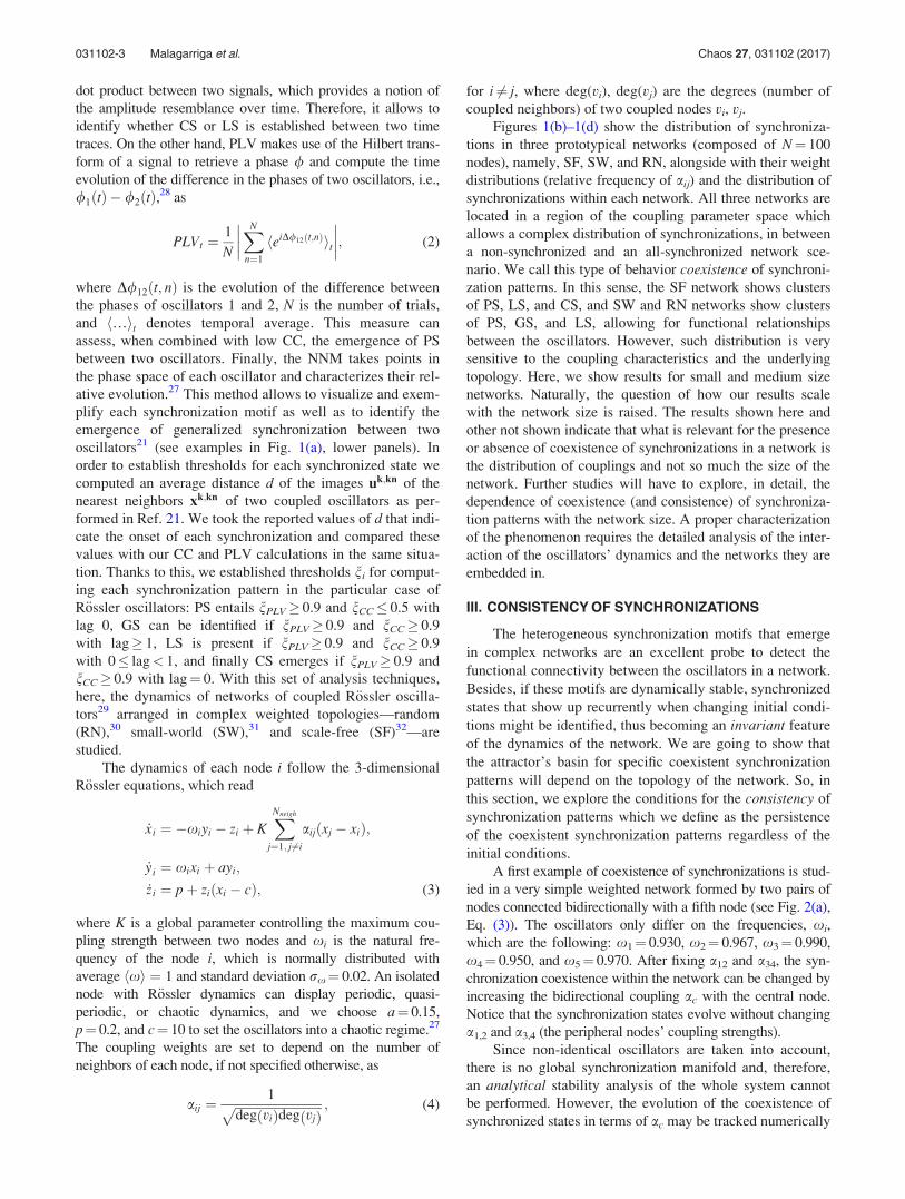
Figure 2(b) shows that, in terms of ac, three different
regions may be defined for the 5 (realization-averaged) larg-
est CLEs, k1xi:
• In the first region (0< ac� 0.06) all the largest CLEs, are
positive. The pairs 1–2 and 3–4 are mostly in PS. When
increasing ac in this region, peripheral nodes become PS
with the central node until the first 0 crossing of k1xi(light
red line), which defines the onset for LS for pair 1–2 (ver-
tical dashed line, first arrow, ac¼ 0.07).• The second region (0.07� ac< 0.23, in between dashed
lines) sets a cascade of coexistence of synchronization
regimes, i.e., successive zero-crossings of CLEs, deter-
mine the onset of GS and LS between the nodes. Notice
that the heterogenous pattern PS/LS is the most frequently
observed. Pattern PS/GS was rare and pattern GS/LS was
never observed.• In the third region, after ac¼ 0.23, there is the onset of LS
for the whole network.
FIG. 2. Dependence of the coexistence
of synchronization patterns on the
Lyapunov Exponents. (a) Simple
weighted network formed by two pairs
of peripheral nodes connected to a cen-
tral node. The couplings between
peripheral node pairs are a12¼ 0.05 and
a34¼ 0.03. (b) For each node dynamics
the curves show the mean value (com-
puted over 100 runs with random initial
conditions) of the maximum Lyapunov
exponent (k1) as a function of the
strength of coupling ac of all nodes
with the central node. The lowest thin
curve corresponds to the lowest values
of k1 for node x1 computed indepen-
dently for each value of ac. This curve
crosses the zero line at ac¼ 0.06, as
indicated by an arrow and a vertical
dotted line. The uppermost thin curve
corresponds to the largest values of k1
for node x2. This curve crosses the zero
line at ac¼ 0.23, as indicated by an
arrow and a vertical dotted line. (c)
Histogram of the occurrences of the
synchronized patterns for each periph-
eral node pair in the network (1–2 and
3–4). Notice that in the interval ac 2[0.06, 0.23] several synchronization
patterns may coexist for the same cou-
pling ac, depending only on the ran-
domly chosen initial conditions.
031102-4 Malagarriga et al. Chaos 27, 031102 (2017)
Figure 2(c) shows the histogram of the occurrence of
each pair of synchronized states between nodes 1–2 or 3–4,
computed using CC, PLV, and NNM: in the coexisting
region, there exist extended ac values for which pairs 1–2
and 3–4 are, simultaneously, in several different synchro-
nized regimes, e.g., 1–2 are in LS meanwhile nodes 3–4 are
in PS. Therefore, for this range of coupling ac, several syn-
chronized states can coexist in the network.
The cascade of zero-crossings of the CLEs, in terms of
ac can be expanded or squeezed by increasing or decreasing
the symmetries of the system, and therefore the range of ac
values for which coexistence appears. For a completely sym-
metrical system, i.e., equal governing equations for all the
nodes in a symmetric network, there are abrupt transitions to
synchrony,34 without coexistence. Symmetry can be broken
in a controlled way by means of a parameter governing the
dynamics (e.g., oscillatory frequency), a parameter responsi-
ble for the topological characteristics of the network (e.g.,
clustering), or both features. In such scenarios different
motifs of synchronized dynamics may show up, but they are
restricted to a tiny region of the parameter space and, hence,
appear to be spurious. Here, symmetry is broken by adding
mismatches between the frequencies of the oscillators and by
increasing the heterogeneity of the nodes’ degrees as well as
the coupling values aij.
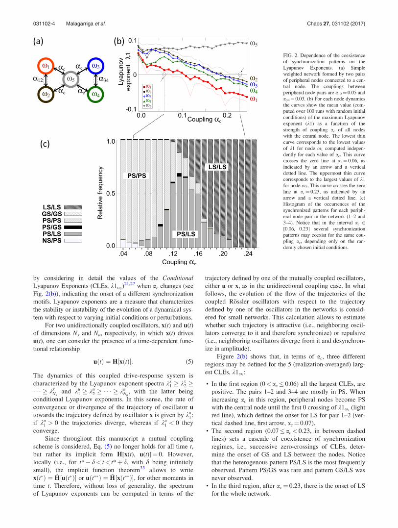
Figure 3(a) shows the motif studied previously, but with
different coupling strengths between peripheral nodes; a1,2 is
now one order of magnitude smaller than a3,4 (see caption of
Fig. 3), making this motif more asymmetrical in terms of
coupling strength. Again, the evolution of the CLEs, is
tracked for increasing ac values. First, for ac¼ 0, nodes 1–2
are in PS meanwhile nodes 3–4 are in GS—i.e., a coexis-
tence situation. As can be seen in Fig. 3(a), for different ini-
tial conditions zero-crossings of CLEs, appear along an
extended ac value region. In this case, the coexistence region
for peripheral nodes 1–2 and 3–4 spans from ac¼ 0 to
ac¼ 0.20. The right panel in Fig. 3(a) shows a plot of the rel-
ative frequency of synchronizations found for each pair of
nodes in the small motif for ac¼ 0.04 (three pointed star)
and ac¼ 0.18 (dotted circle). In the first case, ac¼ 0.04, each
pair in the network lays in the same synchronization state for
any of the imposed initial conditions, whereas in the second
case, ac¼ 0.18, many pairs display different synchroniza-
tions depending on the initial conditions. Consequently, the
first case displays more consistency than the second case
because the network shows the same coexistence pattern
regardless of the initial conditions.
Figure 3(b) shows a more symmetric network, in terms
of coupling strength ac. Such relay configuration is less prone
to synchronize for small coupling strengths and, therefore,
larger ac values are required to set synchronized states (see
inset ac¼ 0.18). Fig. 3(b) lower right panel shows the relative
frequency of synchronizations, with no large predominance of
a single synchronization motif for a given pair of nodes.
Therefore, the motif can be considered non-consistent.Figure 3(c) shows an all-to-all small network in which
all edges are weighted by the control parameter ac. In
this case the network topology and the coupling strength dis-
tribution make this network more symmetrical. Accordingly,
the ac range for which coexistence exists is narrower with
respect to the previous studied motifs. This reduction of the
area of coexistence has implications in the consistency of
synchronizations: zero-crossings of CLEs, are randomly dis-
tributed in a tiny range of ac and, so, coupled pairs in the net-
work do not consistently lay in the same synchronized state
for different initial conditions (see Fig. 3(c) right panel).
Overall, by gathering the results of the coexistence and
the consistency phenomena, we show that network symme-
tries govern the synchronization dynamics emerging from a
system of coupled dynamical units.35 In this regard, clusters
of synchronizations dynamically emerge thanks to symmetry
breaking (with respect to the topology, the system parameter
values, or both) and the statistics of the synchronization
dynamics strongly depend on the type of symmetry breaking.
IV. CONSTRUCTION OF CONSISTENT NETWORKS
Functional networks can be constructed by establishing
relationships between their (coupled) elements. One of the
most prominent dynamical features that functionally relate
two oscillators is synchronization, which may take the afore-
mentioned forms (PS, GS, LS, and CS) among others not
studied here. Therefore, synchronization is a probe for
assessing a (non) trivial relationship between two dynamical
systems. In this sense, in contrast to traditional approaches
where only one type of synchronization is considered, the
statistics of coexistence may reveal a complex functional
organization of synchronization within a network and, there-
fore, may help to construct robust functional networks.
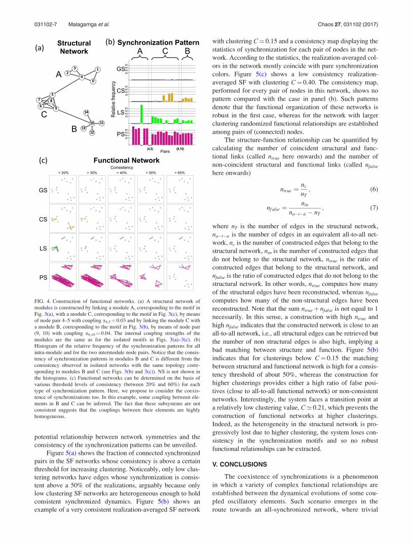
First, the motifs studied in Fig. 3 are coupled through
their hubs (or most connected nodes) to construct a larger
network of dynamical units. The resulting graph is shown in
Fig. 4(a), where each of the motifs is labeled as A, B, or C.
The intra-motif weights are the same as the selected in Figs.
3(a)–3(c), respectively, whereas the inter-hub links weights
are shown in the caption of Fig. 4. Figure 4(b) shows the sta-
tistics of synchronization occurrence in this network: cluster
A shows a very robust consistency of its synchronizations
whereas clusters B and C are much less consistent, i.e., they
display a wide repertoire of different synchronization motifs
depending on the initial conditions. However, as can be
noticed when comparing the relative-frequency plots shown
in Figs. 3(a)–3(c) and 4(b), the dynamics of synchronization
is altered when the three motifs are embedded in a larger net-
work. This fact is a signature for assessing that the dynamics
of coexistence in the large network is not just the simple jux-
taposition of the dynamics of its composite sub-network
motifs.
The construction of the functional networks arising from
the synchronization patterns in this network is performed as
follows: the statistical occurrence of each synchronization
among pairs of nodes of the system is taken into account to
better characterize the most salient synchronization motifs
between the nodes. Then, thresholds in the statistical occur-
rence of each pairwise synchronization are applied, leading
to the extraction of the links which, statistically, appear the
most and so are more consistent.
031102-5 Malagarriga et al. Chaos 27, 031102 (2017)
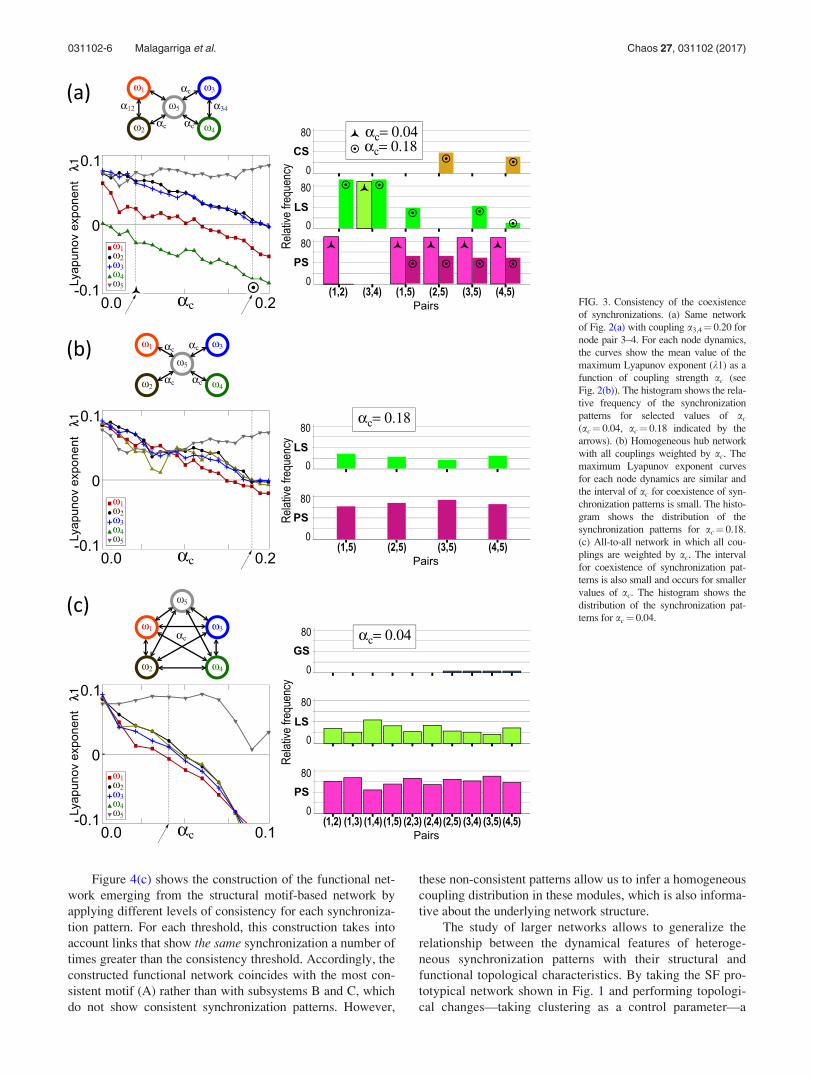
Figure 4(c) shows the construction of the functional net-
work emerging from the structural motif-based network by
applying different levels of consistency for each synchroniza-
tion pattern. For each threshold, this construction takes into
account links that show the same synchronization a number of
times greater than the consistency threshold. Accordingly, the
constructed functional network coincides with the most con-
sistent motif (A) rather than with subsystems B and C, which
do not show consistent synchronization patterns. However,
these non-consistent patterns allow us to infer a homogeneous
coupling distribution in these modules, which is also informa-
tive about the underlying network structure.
The study of larger networks allows to generalize the
relationship between the dynamical features of heteroge-
neous synchronization patterns with their structural and
functional topological characteristics. By taking the SF pro-
totypical network shown in Fig. 1 and performing topologi-
cal changes—taking clustering as a control parameter—a
FIG. 3. Consistency of the coexistence
of synchronizations. (a) Same network
of Fig. 2(a) with coupling a3,4¼ 0.20 for
node pair 3–4. For each node dynamics,
the curves show the mean value of the
maximum Lyapunov exponent (k1) as a
function of coupling strength ac (see
Fig. 2(b)). The histogram shows the rela-
tive frequency of the synchronization
patterns for selected values of ac
(ac¼ 0.04, ac¼ 0.18 indicated by the
arrows). (b) Homogeneous hub network
with all couplings weighted by ac. The
maximum Lyapunov exponent curves
for each node dynamics are similar and
the interval of ac for coexistence of syn-
chronization patterns is small. The histo-
gram shows the distribution of the
synchronization patterns for ac¼ 0.18.
(c) All-to-all network in which all cou-
plings are weighted by ac. The interval
for coexistence of synchronization pat-
terns is also small and occurs for smaller
values of ac. The histogram shows the
distribution of the synchronization pat-
terns for ac¼ 0.04.
031102-6 Malagarriga et al. Chaos 27, 031102 (2017)
potential relationship between network symmetries and the
consistency of the synchronization patterns can be unveiled.
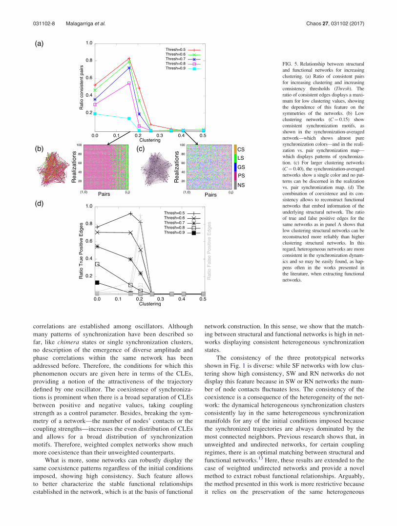
Figure 5(a) shows the fraction of connected synchronized
pairs in the SF networks whose consistency is above a certain
threshold for increasing clustering. Noticeably, only low clus-
tering networks have edges whose synchronization is consis-
tent above a 50% of the realizations, arguably because only
low clustering SF networks are heterogeneous enough to hold
consistent synchronized dynamics. Figure 5(b) shows an
example of a very consistent realization-averaged SF network
with clustering C¼ 0.15 and a consistency map displaying the
statistics of synchronization for each pair of nodes in the net-
work. According to the statistics, the realization-averaged col-
ors in the network mostly coincide with pure synchronization
colors. Figure 5(c) shows a low consistency realization-
averaged SF with clustering C¼ 0.40. The consistency map,
performed for every pair of nodes in this network, shows no
pattern compared with the case in panel (b). Such patterns
denote that the functional organization of these networks is
robust in the first case, whereas for the network with larger
clustering randomized functional relationships are established
among pairs of (connected) nodes.
The structure-function relationship can be quantified by
calculating the number of coincident structural and func-
tional links (called ntrue here onwards) and the number of
non-coincident structural and functional links (called nfalse
here onwards)
ntrue ¼nc
nT; (6)
nf alse ¼nin
na�t�a � nT; (7)
where nT is the number of edges in the structural network,
na�t�a is the number of edges in an equivalent all-to-all net-
work, nc is the number of constructed edges that belong to the
structural network, nin is the number of constructed edges that
do not belong to the structural network, ntrue is the ratio of
constructed edges that belong to the structural network, and
nfalse is the ratio of constructed edges that do not belong to the
structural network. In other words, ntrue computes how many
of the structural edges have been reconstructed, whereas nfalse
computes how many of the non-structural edges have been
reconstructed. Note that the sum ntrueþ nfalse is not equal to 1
necessarily. In this sense, a construction with high ntrue and
high nfalse indicates that the constructed network is close to an
all-to-all network, i.e., all structural edges can be retrieved but
the number of non structural edges is also high, implying a
bad matching between structure and function. Figure 5(b)
indicates that for clusterings below C¼ 0.15 the matching
between structural and functional network is high for a consis-
tency threshold of about 50%, whereas the construction for
higher clusterings provides either a high ratio of false posi-
tives (close to all-to-all functional network) or non-consistent
networks. Interestingly, the system faces a transition point at
a relatively low clustering value, C’ 0.21, which prevents the
construction of functional networks at higher clusterings.
Indeed, as the heterogeneity in the structural network is pro-
gressively lost due to higher clustering, the system loses con-
sistency in the synchronization motifs and so no robust
functional relationships can be extracted.
V. CONCLUSIONS
The coexistence of synchronizations is a phenomenon
in which a variety of complex functional relationships are
established between the dynamical evolutions of some cou-
pled oscillatory elements. Such scenario emerges in the
route towards an all-synchronized network, where trivial
FIG. 4. Construction of functional networks. (a) A structural network of
modules is constructed by linking a module A, corresponding to the motif in
Fig. 3(a), with a module C, corresponding to the motif in Fig. 3(c), by means
of node pair 4–5 with coupling a4,5¼ 0.03 and by linking the module C with
a module B, corresponding to the motif in Fig. 3(b), by means of node pair
(9, 10) with coupling a9,10¼ 0.04. The internal coupling strengths of the
modules are the same as for the isolated motifs in Figs. 3(a)–3(c). (b)
Histogram of the relative frequency of the synchronization patterns for all
intra-module and for the two intermodule node pairs. Notice that the consis-
tency of synchronization patterns in modules B and C is different from the
consistency observed in isolated networks with the same topology corre-
sponding to modules B and C (see Figs. 3(b) and 3(c)). NS is not shown in
the histograms. (c) Functional networks can be determined on the basis of
various threshold levels of consistency (between 20% and 60%) for each
type of synchronization pattern. Here, we propose to consider the coexis-
tence of synchronizations too. In this example, some coupling between ele-
ments in B and C can be inferred. The fact that these subsystems are not
consistent suggests that the couplings between their elements are highly
homogeneous.
031102-7 Malagarriga et al. Chaos 27, 031102 (2017)
correlations are established among oscillators. Although
many patterns of synchronization have been described so
far, like chimera states or single synchronization clusters,
no description of the emergence of diverse amplitude and
phase correlations within the same network has been
addressed before. Therefore, the conditions for which this
phenomenon occurs are given here in terms of the CLEs,
providing a notion of the attractiveness of the trajectory
defined by one oscillator. The coexistence of synchroniza-
tions is prominent when there is a broad separation of CLEs
between positive and negative values, taking coupling
strength as a control parameter. Besides, breaking the sym-
metry of a network—the number of nodes’ contacts or the
coupling strengths—increases the even distribution of CLEs
and allows for a broad distribution of synchronization
motifs. Therefore, weighted complex networks show much
more coexistence than their unweighted counterparts.
What is more, some networks can robustly display the
same coexistence patterns regardless of the initial conditions
imposed, showing high consistency. Such feature allows
to better characterize the stable functional relationships
established in the network, which is at the basis of functional
network construction. In this sense, we show that the match-
ing between structural and functional networks is high in net-
works displaying consistent heterogeneous synchronization
states.
The consistency of the three prototypical networks
shown in Fig. 1 is diverse: while SF networks with low clus-
tering show high consistency, SW and RN networks do not
display this feature because in SW or RN networks the num-
ber of node contacts fluctuates less. The consistency of the
coexistence is a consequence of the heterogeneity of the net-
work: the dynamical heterogeneous synchronization clusters
consistently lay in the same heterogeneous synchronization
manifolds for any of the initial conditions imposed because
the synchronized trajectories are always dominated by the
most connected neighbors. Previous research shows that, in
unweighted and undirected networks, for certain coupling
regimes, there is an optimal matching between structural and
functional networks.13 Here, these results are extended to the
case of weighted undirected networks and provide a novel
method to extract robust functional relationships. Arguably,
the method presented in this work is more restrictive because
it relies on the preservation of the same heterogeneous
FIG. 5. Relationship between structural
and functional networks for increasing
clustering. (a) Ratio of consistent pairs
for increasing clustering and increasing
consistency thresholds (Thresh). The
ratio of consistent edges displays a maxi-
mum for low clustering values, showing
the dependence of this feature on the
symmetries of the networks. (b) Low
clustering networks (C¼ 0.15) show
consistent synchronization motifs, as
shown in the synchronization-averaged
network—which shows almost pure
synchronization colors—and in the reali-
zation vs. pair synchronization map—
which displays patterns of synchroniza-
tion. (c) For larger clustering networks
(C¼ 0.40), the synchronization-averaged
networks show a single color and no pat-
terns can be discerned in the realization
vs. pair synchronization map. (d) The
combination of coexistence and its con-
sistency allows to reconstruct functional
networks that embed information of the
underlying structural network. The ratio
of true and false positive edges for the
same networks as in panel A shows that
low clustering structural networks can be
reconstructed more reliably than higher
clustering structural networks. In this
regard, heterogeneous networks are more
consistent in the synchronization dynam-
ics and so may be easily found, as hap-
pens often in the works presented in
the literature, when extracting functional
networks.
031102-8 Malagarriga et al. Chaos 27, 031102 (2017)
synchronization patterns, but it provides higher robustness to
the constructed functional networks.
The present results, though limited in their scope, also
point towards a general feature in the structure-function rela-
tionship in network science: the construction of functional
networks, for the oscillators used here, bring about heteroge-
neous (non-symmetrical) networks because they are more
consistent. More symmetric or homogeneous networks will
appear as inconsistent if coupling is small: only when cou-
pling is large enough to force global synchronization robust
symmetrical networks will show up in the constructed func-
tional networks. We believe that this structure-function rela-
tionship may also be true for other oscillators. Our result
explains some previous experimental results. For instance, in
brain dynamics, previous experimental studies have shown
that consistent dynamics result in selected network topolo-
gies that have been retrieved much more often than
others.36,37 However, further theoretical and experimental
studies, for other systems, should address this point to limit
or extend the validity of the conclusions raised here.
ACKNOWLEDGMENTS
This work was partially supported by the Spanish
Ministry of Economy and Competitiveness and FEDER
(Project No. FIS2015-66503). AEPV acknowledges support
from the Swiss National Science Foundation Project
NEURECA (CR13I1 138032). J.G.O. also acknowledges
support from the the Generalitat de Catalunya (Project No.
2014SGR0947), the ICREA Academia Programme, and
from the “Mar�ıa de Maeztu” Programme for Units of
Excellence in R&D (Spanish Ministry of Economy and
Competitiveness, MDM-2014-0370).
1A. Pikovsky, M. Rosenblum, and J. Kurths, Synchronization: A UniversalConcept in Nonlinear Sciences (Cambridge University Press, 2003), Vol. 12.
2S. Strogatz, Sync: The Emerging Science of Spontaneous Order (Hachette
Books, 2003).3S. H. Strogatz, Phys. D: Nonlinear Phenom. 143, 1 (2000).4L. Glass, Nature 410, 277 (2001).5D. Abrams and S. Strogatz, Phys. Rev. Lett. 93, 174102 (2004).6I. Omelchenko, Y. Maistrenko, P. H€ovel, and E. Sch€oll, Phys. Rev. Lett.
106, 234102 (2011).
7C. Yao, M. Yi, and J. Shuai, Chaos 23, 033140 (2013).8L. M. Pecora, F. Sorrentino, A. M. Hagerstrom, T. E. Murphy, and R. Roy,
Nat. Commun. 5, 4079 (2014).9L. Schmidt, K. Sch€onleber, K. Krischer, and V. Garc�ıa-Morales, Chaos 24,
013102 (2014).10E. Sch€oll, Eur. Phys. J. Spec. Top. 225, 891 (2016).11M. Chavez, D.-U. Hwang, A. Amann, H. G. E. Hentschel, and S.
Boccaletti, Phys. Rev. Lett. 94, 218701 (2005).12G. Tirabassi, R. Sevilla-Escoboza, J. M. Buld�u, and C. Masoller, Sci. Rep.
5, 10829 (2015).13W. Lin, Y. Wang, H. Ying, Y.-C. Lai, and X. Wang, Phys. Rev. E 92,
012912 (2015).14B. Blasius, A. Huppert, and L. Stone, Nature 399, 354 (1999).15P. A. Robinson, J. J. Wright, and C. J. Rennie, Phys. Rev. E 57, 4578
(1998).16S. Hill and A. Villa, Network: Comput. Neural Syst. 8, 165 (1997).17J. Cabessa and A. Villa, PLoS One 9, e94204 (2014).18D. Malagarriga, A. E. P. Villa, J. Garcia-Ojalvo, and A. J. Pons, PLoS
Comput. Biol. 11, e1004007 (2015).19J. I. Deza, M. Barreiro, and C. Masoller, Chaos: Interdiscip. J. Nonlinear
Sci. 25, 033105 (2015).20D. H. Zanette, Europhys. Lett. 68, 356 (2004).21O. I. Moskalenko, A. A. Koronovskii, A. E. Hramov, and S. Boccaletti,
Phys. Rev. E 86, 036216 (2012).22A. Uchida, F. Rogister, J. Garc�ıa-Ojalvo, and R. Roy, Prog. Opt. 48,
203–341 (2005).23L. Xiao-Wen and Z. Zhi-Gang, Commun. Theor. Phys. 47, 265
(2007).24M. G. Rosenblum, A. S. Pikovsky, and J. Kurths, Phys. Rev. Lett. 76,
1804 (1996).25H. Abarbanel, N. Rulkov, and M. Sushchik, Phys. Rev. E 53, 4528
(1996).26M. G. Rosenblum, A. S. Pikovsky, and J. Kurths, Phys. Rev. Lett. 78,
4193 (1997).27S. Boccaletti, J. Kurths, G. Osipov, D. Valladares, and C. Zhou, Phys.
Rep. 366, 1 (2002).28J. P. Lachaux, E. Rodriguez, J. Martinerie, and F. J. Varela, Hum. Brain
Mapp. 8, 194 (1999).29O. R€ossler, Phys. Lett. A 57, 397 (1976).30P. Erd}os and A. R�enyi, Publ. Math. (Debrecen) 6, 290 (1959).31D. J. Watts and S. H. Strogatz, Nature 393, 440 (1998).32A.-L. Barab�asi and R. Albert, Science 286, 509 (1999).33K. Jittorntrum, J. Optim. Theory Appl. 25, 575 (1978).34I. Leyva, R. Sevilla-Escoboza, J. M. Buld�u, I. Sendi~na Nadal, J. G�omez-
Garde~nes, A. Arenas, Y. Moreno, S. G�omez, R. Jaimes-Re�ategui, and S.
Boccaletti, Phys. Rev. Lett. 108, 168702 (2012).35V. Nicosia, M. Valencia, M. Chavez, A. D�ıaz-Guilera, and V. Latora,
Phys. Rev. Lett. 110, 174102 (2013).36V. M. Egu�ıluz, D. R. Chialvo, G. a. Cecchi, M. Baliki, and A. V.
Apkarian, Phys. Rev. Lett. 94, 018102 (2005).37E. Bullmore and O. Sporns, Nat. Rev. Neurosci. 10, 186 (2009).
031102-9 Malagarriga et al. Chaos 27, 031102 (2017)
Recommended