
Corporate Form and Proprietary Costs of VoluntaryDisclosure
DONALD MONK∗
January 2011
ABSTRACT
Single-segment (focused) firms have a natural disadvantage comparedto multi-segment (diversified) with respect to voluntary disclosure policy.Since aggregate disclosures by focused firms are at a finer level of detailthan those of diversified firms, the latter have greater ability to react tofocused firm information and therefore have a competitive advantage. Iprovide evidence that focused firms are less likely to provide earnings fore-casts even after controlling for typical determinants of forecast issuanceincluding various controls for proprietary costs. This result is the first toshow that corporate form is an additional determinant of voluntary disclo-sure. Tests showing that disclosure ranking is not related to excess valueare inconsistent with the alternative explanation that diversified firmsreap greater benefits of disclosure. However, tests using additional mea-sures of voluntary disclosures (forecast lead time, specificity, and error)are inconclusive.
∗Monk is a Ph.D. Candidate from Tulane University and can be reached via e-mail [email protected].
1. Introduction
When a multi-segment (“diversified”) firm discloses information to the public at the
aggregate level it is, by definition, disclosing less fine information than a single-
segment (“focused”) firm. For example, Microsoft reported five business segments
(plus one Eliminations segment) in its 2008 10-K filing with aggregate sales of $60.4
billion. Google reported just one business segment with total sales of $21.8 billion on
its 2008 10-K. Of Microsoft’s five segments, four of them operate in the same three-
digit Standard Industrial Company (SIC) code (737) as Google’s single segment. If
Microsoft voluntarily discloses a forecast of an aggregate performance measure such
as earnings per share, its competitors would have to make assumptions as to how
those earnings are allocated by segment. On the other hand, if Google voluntarily
discloses such a measure, its competitors are able to assign the forecasted perfor-
mance with more precision and adjust their competitive structure accordingly. The
example points to a potentially lower cost of disclosure for Microsoft due to its diver-
sified status. This study addresses the more general question of whether differences in
voluntary disclosure between diversified and focused firms are related to proprietary
costs after controlling for other determinants of voluntary disclosure.
Much of the voluntary disclosure literature stems from the full disclosure theories
of Milgrom (1981) and Grossman and Hart (1980). These models are based on the
premise that sellers with private information who choose not to disclose will receive
a discounted price, as buyers treat withheld information as less favorable. In this
scenario, it is in the seller’s best interest to reveal all private information in order
to get the best price. Diamond and Verrecchia (1991), Barry and Brown (1985),
and Merton (1987) extend this idea to the context of disclosure by showing that a
commitment to higher levels of disclosure provides a benefit of a lower cost of capital
by decreasing information asymmetry, reducing estimation risk, or increasing investor
following, respectively.1
Verrecchia (1983) develops a model in which concerns of revealing proprietary
information rationally limit voluntary disclosure despite its apparent benefit. In his
1Surveys by Healy and Palepu (2001) [empirical] and Verrecchia (2001) [analytical] provide athorough background of the literature with further discussion of topics too vast to cover in detailhere. Also, reviews of those surveys by Core (2001) and Dye (2001), respectively, offer usefulcounterpoints.
2

model, withheld information cannot be treated unequivocally as less favorable due
to management’s tradeoff between the benefit of a lower cost of capital and the cost
of higher competitive pressure. Unlike in the full disclosure models, traders must
consider proprietary costs as a reason for withholding the information. Thus, they
cannot discount firm value until full disclosure is optimum. Instead, a threshold level
of disclosure is obtained. A firm with higher proprietary costs will enjoy a lower
discount from withholding information. Extending this argument to diversification,
if focused firms have higher proprietary costs as indicated in the Microsoft/Google
example above, traders will react less negatively to withheld information from focused
firms than from diversified firms, all else equal. Knowing that they will not be dis-
counted as severely for withholding information, focused firms have more discretion
to limit their disclosures.
I test whether focused firms adhere to a voluntary disclosure policy that is con-
sistent with higher proprietary costs of disclosure than for diversified firms. First, I
study the determinants of the firm’s decision to issue a forecast with a focus on how
corporate form affects this decision. Specifically, I answer the question: Are focused
firms less likely to issue a guidance forecast? Although many of the aforementioned
theoretical arguments and tests could be applied in the context of mandatory disclo-
sures, I focus on voluntary disclosures because they offer a clear opportunity for a
firm to either reveal or withhold private information. According to Baginski, Conrad,
and Hassell (1993), using management forecasts “has the distinct advantage that the
level of forecast precision is not directly regulated” which provides managers with
some discretion on how they disclose their information.
Using the FirstCall Historical Database of Company Issued Guidance and neces-
sary Compustat data for fiscal years 1994–2008, I show that focused firms are less
likely than diversified firms to issue an earnings forecast, which is consistent with
higher proprietary costs of disclosure for focused firms than for diversified firms. This
result is contrary to research providing support for a negative association between
corporate diversification and disclosure, such as Bens and Monahan (2004). Further-
more, the result presented here is the first to the author’s knowledge to be derived
using FirstCall voluntary disclosure measures and diversification status.2 On average
2In analyzing R&D voluntary disclosures, Jones (2007) shows that the number of segments isnot significantly related to disclosure. Hope and Thomas (2008) also show that the number of
3

over the sample period, greater than 30% of diversified firms issue a forecast in a fiscal
year while less than 22% of focused firms do so. After controlling for other factors
known to affect voluntary disclosure (e.g., growth opportunities, fear of litigation,
earnings volatility, and recent performance), I find that diversified firms are still more
likely to issue a forecast than a focused firm.
Most studies of voluntary disclosures simply use a proxy for proprietary costs to
control for its effects, but the intuitive link between proprietary costs and diversifi-
cation provides another test mechanism. I consider numerous proxies for proprietary
costs, such as the Herfindahl Index, market-to-book ratio, the speed of adjustment to
abnormal profit, and research and development expenses, to compare my results with
those of extant literature. Additionally, I construct two measures of proprietary costs
using the distribution of sales across business segments of the firm: weighted-average
Herfindahl Index and weighted-average market share. Since diversified firms are com-
posed of pieces of different industries with different proprietary costs, these measures
are likely to be better indicators of the exposure that a firm has to competitive pres-
sures. Including proprietary cost measures with proxies for firm diversification status
provides additional understanding of the relationships between voluntary disclosure
and corporate form.
Despite using various proxies for proprietary costs, the results consistently show
that focused firms are less likely to issue guidance. The results also show that higher
proprietary costs are associated with a lower likelihood of providing guidance. In-
terestingly, most of the measures of proprietary costs are not highly correlated, and
in one case, even when a variable is just the segment sales-weighted average of an-
other. More importantly, the inclusion of typical measures of proprietary costs do not
subsume the positive relationship between diversification and voluntary disclosure.
Since voluntary disclosure is argued to lower information asymmetry, I also use
the diversification discount valuation framework to study whether firms that disclose
have higher values than those that do not. If diversified firms have higher informa-
tion asymmetry due to their more opaque form and voluntary disclosure lowers it,
diversified firms may have a greater incentive to disclose if they can reap gains from
the disclosure. In addition to using control variables for information asymmetry in
line-of-business segments does not have explanatory power using measures of voluntary geographicdisclosures as dependent variables.
4

earlier tests to control for such effects, I run additional tests to see if the valuation
impact of disclosure is consistent with the information asymmetry argument.
To test the valuation effects of disclosure, I study its relationship to excess value,
which is the relative value of a diversified firm to its imputed value using data from
focused competitors. Bens and Monahan (2004) lend some credence to the existence of
a relationship between corporate form and disclosure by showing that diversified firms
score lower than focused firms in the AIMR (Association for Investment Management
and Research) disclosure rankings, and their lower ranking is associated with a lower
value for diversified firms relative to focused firms. My data allow me to update
Bens and Monahan’s work with more recent data, new empirical methods, and with
actual disclosures rather than outsider rankings of disclosure. Tests using forecast
lead time, specificity, and absolute forecast error show that increased disclosure is
associated with higher excess value, but only the number of forecasts provided in a
fiscal year is significant when interacted with diversification status. Moreover, results
for forecast error (absolute value and level) support a negative relationship between
disclosure and excess value for diversified firms. Overall, the evidence for particular
valuation effects of disclosure for diversified firms is only weakly supported in my
tests.3
My primary tests are subject to a few econometric concerns that I address us-
ing various methods. First, instead of using the entire Compustat database as the
base sample from which to find nonforecasting matches for the FirstCall sample, I
implement coarsened exact matching. Following Coller and Yohn (1997), I match
firms based on market value of equity, two-digit SIC code, fiscal year, and primary
exchange. Results using this adapted sample fully support the finding that diversified
firms are more likely to issue a forecast.
Another econometric concern is the endogeneity that has been shown in the de-
cision to diversify. Campa and Kedia (2002) and Villalonga (2004) show that the
decision to diversify is endogenous, and this endogeneity can drastically change re-
sults using measures of corporate form. To ameliorate these concerns I use a two-stage
3This result is further complicated by the interpretation of forecast error as a measure of dis-closure. The primary issue is that it is an ex-post measure of how accurate management was inpredicting actual earnings. Increasing the time between forecast and actual earnings (forecast leadtime, which is itself a measure of disclosure) increases the likelihood that confounding factors effectforecast accuracy.
5
framework that invokes instruments for diversification in the first stage and then uses
a predicted value for diversification status in the second stage. The result that a more
diversified firm is more likely to provide guidance continues to hold in most of the
models used.
Two substantial regulatory changes affect my study. First, the regulatory change
from Financial Accounting Standards Board (1976) (hereafter SFAS No. 14) to Fi-
nancial Accounting Standards Board (1997) (hereafter SFAS No. 131) had the stated
intention to increase the transparency of diversified firms. Berger and Hann (2003,
2007) and Botosan and Stanford (2005) study mandatory disclosure differences be-
tween diversified and focused firms surrounding this rule change. Berger and Hann
(2007) report that diversified firms hid segments in ways consistent with agency cost
explanations, but Botosan and Stanford (2005) find that proprietary cost measures
were more prominent in the event. I incorporate this rule change into my analysis
by making necessary adjustments to the segment data to allow for comparison before
and after the rule.
Second, in late 2000 upon the adoption of Regulation Fair Disclosure (Securities
and Exchange Commission (2000); hereafter Reg FD), management was prohibited
from selectively providing material information to outsiders without releasing the
information to the public. Reg FD was accompanied by marked changes in forecasts
provided to the public (Ajinkya, Bhojraj, and Sengupta (2005)). To study the effects
of Reg FD I include an indicator variable to study the time period before and after
the rule was adopted separately. These results show a strong positive relationship
between the adoption of RegFD and voluntary disclosure. The previous result of a
greater propensity to disclose for diversified firms is present, but no longer significant.
A differential effect for diversified firms after RegFD is not evident, though there is
weak evidence of a positive relationship.
After analyzing the propensity to issue a forecast, I turn my attention to the tim-
ing and content of the forecasts. If focused firms have higher proprietary costs of
disclosure, they may obfuscate their forecasts by delaying them, by providing lower
forecast specificity, or by providing less accurate forecasts. Conditional on issuing a
forecast, I test whether focused firms, relative to diversified firms, provide forecasts
with less lead time, with less specificity, or with greater error from actual earnings
when announced. Results for forecast lead time, specificity, and error do not sup-
6

port the proprietary cost hypotheses associated with diversification, though there are
indications of support in summary statistics. The lack of supporting results after
conditioning on a forecast is not surprising given the induced endogeneity of the tests
and additional econometric issues, such as simultaneity of forecast characteristic de-
termination. A more rigorous study of forecast characteristics and their association
with diversification is left for future research.
The remainder of the paper proceeds as follows. Section 2 reviews relevant liter-
ature on voluntary disclosure and corporate form and provides further rationale for
my study. Section 3 continues with a description of the data used in my empirical
analysis. I present the tests and results showing differences in management guid-
ance between diversified and focused firms in Section 4, and I address some empirical
issues. Section 5 concludes.
7

2. Literature Review and Motivation
In the following section I motivate tests of voluntary disclosure differences between
single-segment (focused) firms and multi-segment (diversified) firms. Disclosure pro-
vides management with the means to reveal their private information if they so choose.
In the context of takeover bids, Grossman and Hart (1980) show that a seller with
private information about the quality of the item will reveal his information in equi-
librium, resulting in full disclosure. Similar analytical results can be found in Milgrom
(1981).
This section details how proprietary costs associated with voluntary disclosure
may inhibit full disclosure, and how such costs have been shown to limit disclosure.
With the support of the literature in conglomerate diversification and voluntary dis-
closure, I argue that focused firms have a higher proprietary cost of disclosure and
therefore disclose less than diversified firms. Also, I consider potential alternatives to
the proprietary cost hypotheses.
A. Proprietary Cost Hypothesis
Early explanations for non-disclosure hinged on the assumption in the full disclosure
models that the information could be conveyed with little or no cost. Later models
show that the benefits of lowering information asymmetry and potentially lowering
the cost of capital via disclosure could be offset by costs of the disclosure. In the
informational setting where a value maximizing manager with private information
chooses whether to reveal his information, models by Verrecchia (1983) and Bhat-
tacharya and Ritter (1983) yield the full disclosure result for low-cost information,
but their models provide for a threshold level of disclosure when such information
production is costly.4
4Diamond (1985) provides an explanation for investor demand of such information. A basicpremise of much of accounting literature and of the full disclosure literature in particular is thatmanagers possess private information and investors know this fact. In practice, this assumptionseems believable, although surely there are cases in which management knows little or no information.Myers and Majluf (1984) offers a well known example of a financial model assuming that agents havesuperior information. On the other hand, Axelson (2007) develops a security design model in whichbidders have superior information to management.
8

Verrecchia (1983) pinpoints proprietary costs as a mechanism to model the trade-
offs of disclosure. In his model, firms choose to disclose information based on an
expected reaction by traders to the disclosure or non-disclosure. If the expected detri-
ment is more than the benefits, the disclosure should not rationally occur. His model
predicts a negative association between product market competition and disclosure.
In the presence of proprietary costs, traders are unable to assess whether the lack of
disclosure is good news or bad news, and the full disclosure premise is no longer valid.
Other analytical studies addressing proprietary costs make it clear that the type of
competition could be an important factor. For example, Darrough and Stoughton
(1990) study a potential entrant as the form of competition, and their model predicts
that this sort of competition encourages disclosure, therefore predicting a positive
association between threat of entry and disclosure.5
While there is a substantial analytical literature studying the importance of the
proprietary costs of disclosure, empirical evidence is limited. In a review of the
empirical disclosure literature, Healy and Palepu (2001) state that “there is little
direct evidence on the proprietary cost hypothesis.” Verrecchia (1983) predicts that
disclosure and proprietary costs should have a negative relationship, and there seems
to be some support for this prediction. Bamber and Cheon (1998) find that higher
product market competition is related to a lower probability of a firm offering a
forecast in a venue with more “visibility.” This negative relationship extends to the
specificity of the forecast. Moreover, Brockman, Khurana, and Martin (2008) report
a negative relationship between a measure of how far management’s forecast missed
actual earnings-per-share and market-to-book (MB), with MB being their proxy for
proprietary costs (as is also the case in Bamber and Cheon (1998)).
Focused firms that voluntarily disclose private information are revealing a finer
level of detail than diversified firms that reveal aggregate information. For example,
providing a forecast of earnings per share for a focused firm will allow competitors to
assess how that particular business is performing and make adjustments to investment
accordingly. Diversified firms, on the other hand, can provide an earnings forecast for
the consolidated firm without revealing how individual components of the business
5Dye (2001) demonstrates how a market characterized by perfect competition can also lead to apartial disclosure result. He also states that perfect competition is not necessary to increase efficiencyif disclosures help to improve pricing that improves capital allocation. He dubs this the “feedback”effect of disclosure.
9
are performing. Of course, competitors of diversified firm information will be able
to use historical or contemporaneous information about the segments of the firm to
apportion aggregate earnings. However, such apportionment is at best equal to the
apportionment possible with a focused firm. To the extent that competitors are suc-
cessful in apportioning such information, proprietary cost effects will be diminished.6
The potential informational advantage for the diversified firm could raise the costs of
disclosure for a focused firm and motivate the focused firm to refrain from providing
guidance, which is formalized in the following hypothesis in alternate form:
Hypothesis 1. Focused firms are less likely to provide an earnings forecast.
Hypotheses 1 considers the relationship between diversification and voluntary dis-
closure, but an explicit treatment of the competitive environment will provide further
understanding. If the explanatory variable that measures corporate diversification is
simply a noisy proxy for proprietary costs of disclosure in tests of voluntary disclosure
propensity, the inclusion of variables that are more direct proxies for proprietary costs
should decrease the explanatory power of the diversification variable. However, the
diversification variable should still capture proprietary cost differences that are not
captured in standard measures. Specifically, diversified firms should be more likely
to disclose.
B. Evidence from Mandatory Disclosures
Public firms have been required to disclose certain segment information since the
passage of SFAS No. 14 with a considerable update to the rule adopted in 1996 as
SFAS No. 131. The latter rule explicitly addresses competitive harm that may result
from the increase in filing requirements for firms with multiple segments. Most of
the arguments taken from comments to FASB on the implementation of the rule are
concerned with the competitive harm to public diversified companies that are required
to provide segment-level information versus private firms that do not have to disclose
6Hutton, Miller, and Skinner (2003) show that firms provide supplementary statements concur-rently with earnings forecasts approximately two-thirds of the time in their sample; the distributionof statements is almost equal between “good” and “bad” news; and the market only reacts to “good”news forecasts when accompanied by supporting verifiable statements. These results are based onaggregate statements only and do not incorporate the intricacies of diversified versus focused disclo-sure.
10

such information. The Board includes some provisions intended to ameliorate the
competitive harm between public and private diversified firms, but nothing directly
addresses the competitive harm to focused firms that must disclose more than is
required of segments of diversified firms that I hypothesize. In fact, SFAS No. 131
paragraph 111 provides an indication that the competitive pressures faced by segments
of diversified firms and focused firms may be equal:
The Board concluded that it was not necessary to provide an exemption for
single-product or single-service segments because enterprises that produce
a single product or service that are required to issue general purpose
financial statements have that same exposure to competitive harm.
The evidence on the proprietary costs of mandatory disclosure and diversification
is not as limited as the voluntary disclosure side due in part to the rule change men-
tioned in the paragraph above. SFAS No. 131 has the stated intention to increase
transparency by changing the reporting basis from one of industry allocation of seg-
ments to one of operating segments, among other changes. Berger and Hann (2003)
provide evidence supporting an increase in transparency due to the rule change: the
number of reported segments increased and the newly reported information was not
previously incorporated into market expectations or analysts’ predictions. Even with
the advent of the new rule, filings for segments of diversified firms are not as revealing
as those of a firm with just one segment. Required items for segment reporting are
limited to a few items from the income statement used to create a measure of profit
or loss. Focused firms must report consolidated firm filings (via SEC forms 10-K or
10-Q) including such items as research and development and risk factors that can be
used to assess the growth potential of their singular business. Botosan and Stanford
(2005) show that in the previous regime firms hid profitable segments in less compet-
itive industries, which is consistent with competitive pressures impacting mandatory
disclosure. Finally, Berger and Hann (2007) use the same rule change and find that
agency costs rather than proprietary costs appear to influence management’s filing
disclosures.
Other research on mandatory disclosures does not utilize the rule change. Rather,
it focuses on aggregation choice in the presence of competitive pressures. Hayes and
Lundholm (1996) model the decision to aggregate business segments considering the
11
incentives of the firm to reveal or hide disclosures in the presence of a competitor.
They find that a firm faced with a rival has the incentive to aggregate segments that
have disparate results and disaggregate segments when their results are similar, lest
the rival discovers the more profitable business to cannibalize. Harris (1998) compares
SIC codes taken from filings and matches against SIC codes reported in Compustat as
a segment to show that firms tend to aggregate segments in less competitive industries,
although she admits that she finds this result in mandatory disclosures while many
of the models used to motivate her story are for voluntary disclosure.
I adjust my tests for the potential impacts that mandatory disclosures have on a
firm’s complete disclosure environment. First, I adjust the segment data before and
after the adoption of SFAS No. 131 to address pseudo-conglomeration as discussed
in Sanzhar (2006). In addition, Compustat has back-filled segment data before the
1997 to be in accordance with the new filing requirements. Second, I consider the
adoption of Regulation Fair Disclosure (Reg FD) in late 2000. Reg FD prohibited
management from selectively providing material information to outsiders without
releasing the information to the public, and it was accompanied by a marked increase
in the number of forecasts provided to the public as shown in Healy (2007).
C. Consideration of Alternatives
C.1. Cost of Capital
In the full disclosure model, managers are endowed with private information and
investors know that the manager possesses such information. If this information is
disclosed, the information asymmetry between managers and investors diminishes.
Diamond and Verrecchia (1991) show that this reduction leads to a lower price im-
pact on the firm’s securities that increases demand from large investors and in turn
decreases the cost of capital for the firm. Another line of research that produces a
negative relationship between disclosure and cost of capital centers around estimation
risk. In the models of Coles, Loewenstein, and Suay (1995) and Barry and Brown
(1985), firms that offer more information have parameters that are easier to estimate,
resulting in lower market betas and lower expected returns (i.e., lower cost of equity
capital). By modeling information as a noisy indicator of future cash flows, Lambert,
12

Leuz, and Verrecchia (2007) show that increasing the quality of disclosures creates
effects within a CAPM framework that ultimately lead to a lower cost of capital.7
The empirical literature examining the notion of a negative relationship between
disclosure and cost of capital offers mixed results. Botosan and Plumlee (2002) find
support using analysts’ ratings of disclosure of annual documents, but they find a
positive relationship using the ratings of quarterly reports. Brown and Hillegeist
(2007) find more consistent support by showing that annual, quarterly, and investor
relations ratings are negatively related to the probability of informed trade measure
(PIN), which they argue proxies for information asymmetry. Further, Lang and Lund-
holm (1996) show that many measures often used to proxy for information asymmetry,
such as analyst coverage and forecast dispersion, accuracy, and variability, are cor-
related with disclosure in ways that indicate lower information asymmetry for firms
with more disclosure, which is consistent with lower cost of capital.8 Botosan, Plum-
lee, and Xie (2004) argue that public information could either be a complement to
or a substitute for private information, and when they include public information,
the relationship between cost of equity capital and private information is positive. In
support of the price impact story of Diamond and Verrecchia (1991), Coller and Yohn
(1997) show that information asymmetry as measured by bid-ask spreads is higher
for firms providing a forecast than for non-forecasting firms in the period prior to the
forecast, but there is no difference in spreads after a forecast. Also they show that
spreads over the nine days prior to a forecast are significantly higher than the spreads
over the nine days after the management forecast.
Greater disclosure for diversified firms could be a result of an increased incentive
to lower their information asymmetry (and their cost of capital) rather than a result
of lower proprietary cost. The transparency hypothesis offered in Hadlock, Ryngaert,
and Thomas (2001) states that diversified firms have higher information asymmetry
due to lower transparency in the information available about the segments of the firm
7Shin (2006) develops a model incorporating joint determination of asset returns and disclo-sure with predictions that resemble short-term momentum and long-term reversal in returns, but areduction in cost of capital is not the driver of the model.
8While the focus here is on voluntary disclosures that lower information asymmetry, other firmactions that lower information asymmetry have also been shown to be negatively related to costof capital. For instance, Barth, Konchitchki, and Landsman (2008) find that more transparentearnings, that is, earnings that more closely relate to returns, are associated with a lower cost ofcapital.
13

relative to pure-play firm information. The empirical evidence on higher information
asymmetry in diversified firms generally finds the opposite, however. Using analysts’
forecasts as a proxy for information asymmetry, Thomas (2002) shows that diversified
firms do not have more information asymmetry than focused firms. He shows “that
greater diversification is associated with smaller forecast errors and less dispersion
among forecasts.” Moreover, he finds that diversified firms have higher earnings
response coefficients (ERC) indicating that investors impound earnings information
into stock prices to a greater extent than for focused firms. However, the results from
Thomas (2002) indicating lower information asymmetry for diversified firms flip after
controlling for return volatility. Using market microstructure measures of information
asymmetry, Clarke, Fee, and Thomas (2004) support the Thomas (2002) findings of
lower information asymmetry for diversified firms.9
Whether or not diversified firms have a lower cost of capital relative to focused
firms has yet to be fully answered. Only a few studies offer tests related to differences
in cost of capital or expected returns between diversified and focused firms. Hadlock,
Ryngaert, and Thomas (2001) show that relative to focused firms, diversified firms
suffer a less negative stock price reaction to seasoned equity offerings than focused
firms, which is inconsistent with higher levels of information asymmetry for diversified
firms. The authors attribute their result to lower adverse selection problems in issuing
securities of diversified firms due to lower measurement error from imperfectly cor-
related segments than from a bucket of focused segments. If the lower measurement
error for diversified firms that are selling securities is actually due to a commitment
to disclosure above and beyond that of focused firms, increased disclosure could be
causing this result. Lamont and Polk (2001) bring lower cost of capital for diversified
firms into question by showing that there is no difference in returns between diversi-
fied and focused firms, but they do find that discounted diversified firms have higher
realized returns than premium diversified firms.10
I address the possibility that diversified firms have a greater incentive to disclose
due to differences in information asymmetry rather than proprietary cost differences in
9Though not a study including all diversified firms, Krishnaswami and Subramaniam (1999) showthat firms that engage in a spinoff have higher information asymmetry than a matched control groupand gains associated with the spinoff are related to the decrease in information asymmetry for spinofffirms.
10Mitton and Vorkink (2008) find that diversified firms have lower skewness in their returns andthis is consistent with investors’ preference for skewness risk and with a discount for diversified firms.
14

two ways. First, in regressions of disclosure on diversification status and proprietary
costs, I include variables that control for information asymmetry. Next, I analyze
whether firms that provide voluntary disclosure have higher valuations relative to
their industry peers and whether this result is related to diversification status. If the
latter is true, it is an indication that further analysis is needed to disentangle the
determinants of disclosure and how those determinants affect value.
Bens and Monahan (2004) report that disclosure ranking measured using AIMR
ratings, which is used as an inverse proxy for information asymmetry, is positively
associated with excess value, which is measured as a log ratio of the actual value
of a firm to its value imputed from focused firm rivals, for diversified firms, but
the relationship does not exist for focused firms. The authors attribute the positive
association for diversified firms to the increased monitoring that is present for firms
with more revealing disclosure. My empirical structure allows me to update Bens
and Monahan’s work with more recent data, new empirical methods, and with actual
disclosures rather than outsider rankings of disclosure. I test the following hypothesis:
Hypothesis 2. Higher measures of voluntary disclosures are associated with higher
excess value.
Moreover, if diversified firms have higher information asymmetry and use volun-
tary disclosure to decrease it, there would be a positive interaction effect for diver-
sification status and disclosure in regressions of excess value. The hypothesis below
formalizes this argument:
Hypothesis 3. Higher levels of disclosure positively effect the excess value of diver-
sified firms more than focused firms.
C.2. Agency Costs
There is also a strand of literature addressing managers acting in their own interest
and adopting a disclosure policy accordingly. Berger and Hann (2007) provide empir-
ical support for an agency cost story that managers of diversified firms seek to mask
inefficient behavior among their segments by aggregating segments with poor perfor-
mance. Using proxies for disclosure, Aboody and Kasznik (2000) find evidence that
is consistent with firms adapting their voluntary disclosures in favor of CEO option
15

payoffs. Brockman, Martin, and Puckett (2008) lend more support to this argument
by showing that firms release information intended to increase management’s stock
option payoff by releasing positive disclosure before intended exercise of options and
by releasing negative information before intended holding of vested options. In a sim-
ilar agency cost story, insider transactions are shown to be clustered after voluntary
disclosures that result in higher payoffs for the insiders in Noe (1999). Bernhardt and
Campello (2007) provide evidence that managers “talk down” the consensus analyst
estimate of earnings. While this practice fools investors in that they treat the changes
in analysts’ estimates as unbiased, the earnings “surpise” is not substantial enough
to raise the stock price above its losses from talking down the consensus before the
earnings announcement. Finally, Brockman, Khurana, and Martin (2008) show that
managers “talk down” the price of the firm’s stock using voluntary disclosures prior
to repurchasing shares, and the bias in management forecasts is positively correlated
with management’s private incentives.11
Many studies on corporate form point to potential agency costs differences between
diversified and focused firms. At the level of the CEO, Shleifer and Vishny (1989)
model an empire building CEO who overinvests in projects to carve out more rents
for herself. Jensen (1986) details another form of overinvestment borne of greater ac-
cess to free cash flows in the diversified corporate form. Rajan, Servaes, and Zingales
(2000) develop a model in which incomplete contracting on investment choice drives
self-interested divisional managers to invest in projects that are defensive rather than
those that are most efficient for the firm. Scharfstein and Stein (2000) show how
rent-seeking managers provide another avenue for a value loss for corporate diversifi-
cation as managers take on projects that increase their bargaining power rather than
increasing firm value. Lamont (1997), Lamont and Polk (2002), and Ahn and Denis
(2004) provide empirical support for overinvestment by diversified firms. If managers
are behaving in the manner described in these studies, agency costs will be higher
in all cases for diversified firms. As such, they will be considered “lemons” in the
marketplace, and any attempt to mitigate agency costs using disclosure will be moot
11It could be that the adjustment to disclosure by diversified firms is less than for focused firmsbecause investors don’t know enough details to apportion the news to the segments that make upthe business. If this is the case, the good news/bad news studies will have more focused firms inthem, and in turn, those samples will be smaller and younger than excluded firms. Also, dividingthe sample based on ”substantial news” (>1% or <-1% move in price) amplifies the aforementionedeffect.
16

in equilibrium. Since the mechanism by which voluntary disclosures could be used to
mitigate this aspect of differences in corporate form is not evident, I do not include
agency cost considerations in my tests.
17

3. Sample and Variable Construction
The primary data that I use to test the hypotheses are derived from the intersection
of the FirstCall Company Issued Guidance (CIG) database and segment- and firm-
level data from Compustat. A download from CIG with announcement years from
1990–2009 yields 111,908 observations of management forecasts.12 There are only
67 forecasts from 1990–1993, so I remove forecasts announced in those years. Since
announcements pertaining to fiscal year 2009 have yet to be fully incorporated into
the database as of this draft, I also remove forecasts provided during firm fiscal years
after 2008. After choosing forecasts of earnings per share on common stock in U.S.
dollars that possess an eight-digit CUSIP and a FirstCall code that is necessary to
qualify the specificity of the forecasts, the database has 97,975 observations. Similar
to Anilowski, Feng, and Skinner (2007), I remove forecasts that are more than 90 days
after or more than two years and 90 days before the subject fiscal period end of the
forecast. Finally, I remove a few remaining duplicates in CIG for a resulting database
with 94,600 observations (46,184 annual forecasts and 48,416 quarterly forecasts)
spanning fiscal years as of the announcement of 1994–2008 as shown in Table 1.
To derive measures of corporate diversification and to weight variables accord-
ing to segment distribution, I use the segment-level data from Compustat. SFAS
No. 14 created the regulatory requirement for firms to file segment-level information
with implementation and data entries beginning in earnest in the fiscal year of 1978.
Restatements of segment or firm information are removed so the database contains
information that was available to investors at the time of filing rather than adjusted
numbers and filings revealed later.13 I remove financial firms and utilities from the
sample as these industries are regulated differently from others, which could affect
the interpretation of proprietary costs and diversification.
SFAS No. 131 creates the need to make an adjustment to the data on both sides of
the rule change for comparability. I perform the procedure described in Hund, Monk,
12Chuk, Matsumoto, and Miller (2009) note some problems with the CIG database. First, theyshow that hand-collected guidance from Lexis-Nexis is often not present in CIG. Though this maybias my results for the propensity to provide a management forecast, other tests and techniques areemployed to lessen this problem. Also, they show that non-EPS measures and more complicatedcalculations of guidance (e.g., 10% increase in earnings) are not as complete. I use only EPS forecasts.
13To the extent that managers knowingly provide incorrect forecasts and then manipulate filingsto meet the incorrect forecasts, using non-restated data could bias my results.
18
and Tice (2010) to account for the segment reporting changes. The new rule requires
firms to report segments based on operating structure rather than industry compo-
sition. As a result, firms reported more segments, but many of these segments are in
the same four-digit SIC code (see Sanzhar (2006) for details on these pseudoconglom-
erates.) The procedure I use aggregates sales for segments in the same 4-digit SIC
code thereby making the data after SFAS No. 131 more comparable to those before
it. I also remove segments with sales equal to zero or with missing values, since many
of these are “corporate” segments put in place to allow firms (under the new rule)
to allocate assets to the corporate entity rather than business-line segments. Finally,
Compustat has adjusted observations in the segment database before the adoption
of the rule to be in accordance.14 In addition, Compustat created “new” segments
data to backfill years prior to 1997 in their database to provide better comparability
across the regulatory regimes.
Finally I merge the forecast and segment data with Compustat firm-level data
required to perform additional screens for the segment-level data and to calculate
other variables used throughout the study as controls. I remove those firms not
reporting segment sales that sum to within 1% of reported total sales. This firm-level
screen is taken from Berger and Ofek (1995) and is in agreement with the empirical
diversification literature. Other variables will be described in the sections below as
needed. Short descriptions of all variables are in Appendix A.
A. Management Forecasts
Using the FirstCall Company Issued Guidance data described above I create manage-
ment forecast variables for my tests. To get a better sense of how often the firm offers
voluntarily disclosures, I calculate the number of forecasts provided by a firm in fiscal
year t, notated by NForecastt, including updates but not duplicating forecasts given
on the same day. Botosan and Plumlee (2002) find substantial differences between
disclosure rankings based on annual and quarterly reports. Therefore, I produce sep-
arate results for annual and quarterly data where appropriate. I also create a dummy
variable (Forecast) to indicate whether management issued a forecast. Forecast
14Due to the subjective nature of asset allocation under the new rule, I only use segment salesdata in my analysis.
19

equals 1 for each CIG observation that has a matching firm-year observation from
Compustat, and it equals zero for Compustat firm-years that do not have a matching
observation in CIG.
To allow for deeper analysis of the disclosure policy of firms, I create variables
based on more than just the sheer number of management forecasts. First, I calculate
the number of days between the announcement date and the fiscal period end, denoted
by Lead. Note that this variable is negative for those forecasts that are provided after
the fiscal period end but before the actual earnings are announced. To capture the
information available to investors at the time of the announcement and to reduce
erroneous data points, I remove announcements that are more than 90 days after
or more than 820 days (two years plus 90 days) before the subject fiscal period
end. I chose 90 days after the fiscal period end so as not to interfere with results
from the next quarter. I chose two years plus 90 days before the fiscal period end
after looking at the distribution of forecasts and noting a few outliers that were
thousands of days before the fiscal period end and are likely data entry errors. Second,
I create a variable to denote the specificity of forecasts, Spec, using the definitions
from Baginski, Conrad, and Hassell (1993) and a numbering scheme that is increasing
in specificity as indicated in Appendix B. Fig. 2 shows that the number of forecasts
per year peaked in 2004 and that the proportion of “range” forecasts has increased
over time.
The final forecast measure is the ex-post accuracy of the management forecast.
Error is calculated as the difference between the management forecast and actual
earnings normalized by the stock price at the end of the most recent quarter, mul-
tiplied by 100, and winsorized at the 1% level. I also use the absolute value of this
measure in some tests. Ajinkya, Bhojraj, and Sengupta (2005) and Brockman, Khu-
rana, and Martin (2008), among others, use a similar measure of management “bias”
in situations of monitoring and repurchasing shares, respectively. In the present con-
text the measure will be useful in determining if the bias from other research is related
to the effects of proprietary costs and diversification. However, this measure is imper-
fect because for open-interval forecasts, I simply subtract actual EPS number from
the EPS forecast. Also, for range forecasts, I use the mid-point of the range forecast
as management’s forecast following Baginski, Conrad, and Hassell (1993).
20

B. Measures of Diversification Status and Value
Using the Compustat segment data I create two measures of diversification. The
first and most commonly used is the diversification indicator variable (Multit) that
equals one if a firm reports multiple segments by four-digit SIC code in fiscal year
t. Otherwise, the indicator equals zero. To provide additional depth to the analysis,
I also create entropy (Entropyt) as described in Jacquemin and Berry (1979) as a
continuous measure of diversification. The entropy measure of diversification for firm
i is determined at fiscal year t by
Entropyi, t =n∑
s=1
Ps, i, t ln1
Ps, i, t
, (1)
where n is the number of four-digit SIC code segments and Ps, i, t is the proportion of
sales from segment s of firm i at t. Entropy equals zero for firms reporting a single
business segment, and it is greater than zero for firms reporting multiple business
segments. Importantly, entropy changes as the distribution of sales across segments
changes, even if the number of segments is held constant, which allows for an analysis
of the impact of the degree of diversification on disclosure decisions.
Table 2 shows descriptive statistics for annual forecasts split into two panels based
on diversification status. The mean number of annual forecasts per firm per year
(NForecast) has increased from about one in 1994 to above five in 2008, and mean
NForecast is greater for diversified firms in every year after 1997. Diversified firms
comprise only 19% [11, 264/(11, 264+46, 870)] of firms not providing annual guidance,
but they comprise 33% [3, 130/(3, 130+6, 480)] of firms providing an annual forecasts
and 36% [10, 461/(10, 461 + 18, 556)] of total annual forecasts. Similar results for
quarterly forecasts are available upon request.
The similarities between the full FirstCall sample and the screened sample in
unreported tests provide confidence that screening mechanisms did not introduce
substantial bias. In addition, a matching technique is employed in Section 4.B.3 to
provide further empirical support.
21

C. Proprietary Costs
Several measures are needed for reliable proxies for the proprietary costs that firms
face. As noted in early literature cited in Section 2, the type of competition can and
does have an impact on voluntary disclosure equilibrium outcomes. The difference
between product market competition and the threat of entry has been shown to be
enough to change the effect of competition on voluntary disclosures. The variability of
proxies for proprietary costs across industries, firms, and segments can be drastically
different. I separate the measures according to their variability: industry-, firm-, or
segment-level.
C.1. Industry-Level Measures
Following Botosan and Stanford (2005) and Harris (1998), for each three-digit firm-
level SIC code I construct the four-firm concentration ratio (Conc4Firm) and the
Herfindahl Index (HI). The former equals the sum of the proportion of annual sales
in a three-digit SIC code industry of the top four producers by sales, whereas the latter
is the sum of the squared proportions of sales coming from all firms in a three-digit
SIC code industry.15 As these measures increase, competition decreases.
As the last industry-level measure, I use the speed of profit adjustment. Harris
(1998) notes that this measure provides an indicator of the persistence of abnormal
profits away from the industry mean. The value for speed of adjustment, SpeedAdj,
is the coefficient β2j of Eq. 2, which is executed separately for each industry j. As
with Conc4Firm and HI, a higher value for SpeedAdj implies less competition.16
Xijt = β0j + β1j(DnXijt−1) + β2j(DpXijt−1) + εijt (2)
15Ali, Klasa, and Yeung (2009) provide evidence that industry concentration measures usingCompustat can be biased. Their study cites the lack of private firms in the Compustat database asa weakness. However, in the context of testing differences in voluntary public disclosures that areultimately verifiable due to mandatory filings, using only public firms should have less of an impacton inference.
16Berger and Hann (2007) use segment abnormal profitability to proxy for management’s desireto withhold segment information from potential entrants. As stated in their paper, such measuresfor the entire sample of segments are difficult to obtain and to verify. Their sample is limited tofirms changing corporate form around a rule change. As such, they could hand-collect the necessarydata more easily.
22
where
• X is the difference between the ROA of firm i and the mean ROA of its three-
digit SIC industry j;
• Dn is a dummy indicating negative X;
• Dp is a dummy indicating positive X.
C.2. Firm-Level Measures
The equity market-to-book ratio (MB) has been used in the disclosure literature
as a measure of growth opportunities and more loosely as a proxy for proprietary
costs. Firms with high growth opportunities may have a lower incentive to disclose as
argued in Bamber and Cheon (1998), but this relationship could be in the opposite
direction if a firm desires to deter entry by signalling that a particular industry has
lower opportunities. Perhaps this ambiguous relationship is demonstrated in their
findings that the lagged value of MB is negatively associated with the level of investor
proactivity of the release venue, but when used as an explanatory variable for forecast
specificity the ratio is no longer significant. Further, Ajinkya, Bhojraj, and Sengupta
(2005) include lagged MB in similar regressions of management forecasts issuance,
but in most cases their tests show that the coefficient for it is not significantly different
from zero. I calculate MBt as the log of the ratio of the market value of equity at
calendar year end t to the book value of equity.
Other firm-level variables offer more direct proxies for proprietary costs. Research
and development expense (RD), calculated as the yearly R&D expense over assets, is
argued to be positively related to proprietary costs in Wang (2007). In cases in which
R&D expense is missing, I set the value equal to zero. Also, I include three-digit SIC
industry percent rank of profit margin (PMargin) and market share (MShare) as
in Nichols (2009).
C.3. Firm-Level Measures Using Segment-Level Information
Since a diversified firm is composed of multiple segments from potentially multiple
industries, I construct some firm-level variables that are based on segment-level in-
formation. For each measure, I treat the segment as a separate entity within an
23

industry and calculate market share information accordingly. By treating each seg-
ment as a separate competitor in the industry market, these measures offer a more
complete picture of the level of competition that a particular industry participant is
facing. Specifically, I use segment sales and their accompanying industry designation
to create a segment-sales weighted average market share (MShareSeg) and Herfind-
ahl Index (HIwtd). To calculate the latter measure I multiply the proportion of firm
sales in a particular three-digit segment industry by the Herfindahl Index created
using sales values from all segments within a three-digit SIC code industry and then
sum over the number of segments in the firm as shown in Eq. 3 and Eq. 4.
HIsegj =m∑i=1
(siSj
)2 (3)
HIwtdf =n∑
k=1
(skSf
) ∗HIsegj, (4)
where
m = number of segments in three-digit industry j,
s = segment sales,
S = sales from all segments (in industry j or firm f),
n = number of segments in firm f .
Table 3 provides some support for separate consideration of the proprietary cost
measures. Although many of the correlation coefficients between the measures are
significantly different than zero, only four have an absolute value greater than 0.5.
SpeedAdj, MB, and PMargin have very little relationship with any of the other
measures. Since MB has been used in the disclosure literature to proxy for other
economic effects such as growth opportunities, it will remain in my analyses. Among
the remaining proprietary cost proxies, I will consider measures that include industry-
level, firm-level, and segment-based calculations where appropriate.
D. Other Variables
I address two common controls first. Firm size may have a positive or negative
association with disclosure. On one hand, larger firms will have the real resources
24

to produce the information more easily (Diamond (1985)). On the other hand, more
information is generally available publicly for larger firms, perhaps substituting for
some of the information that management would otherwise release (Brockman, Khu-
rana, and Martin (2008)). Harris (1998) argues that firm size is also a proxy for the
number of segments reported due to filing requirements based on a 10% threshold to
list a segment separately. To control for these possible effects I use the variable Size,
measured as the log of total assets. Brown and Hillegeist (2007) also note the im-
portance of recent performance on a firm’s decision to issue guidance. To capture
recent performance I use return on equity, ROE. Using excess firm returns over the
CRSP value-weighted index during the three months ending before the issuance of
the management forecast yields similar results.
Earnings volatility has been used as a measure of the potential for large move-
ments in management forecasts and susceptibility to litigation. Managers from firms
with higher earnings volatility may have a tougher time forecasting earnings and may
be more likely to get the forecast wrong. Not only is this measure applicable in
the study of voluntary disclosures, but also it has been shown to be an important
determinant in studies of corporate diversification. Diversified firms are shown in
Dimitrov and Tice (2006) and Hund, Monk, and Tice (2010) to have significantly
lower volatility in firm performance measures such as ROE, ROA, and EBIT . I
calculate earnings volatility, EarnV ol, as the standard deviation of the previous 12
quarters of earnings before the period including the forecast winsorized at 1%.
To address information asymmetry, which is one of the primary theoreti-
cal determinants of disclosures, I use a few measures taken from extant literature.
First, I use residual stock return standard deviation, V olatility, as calculated in
Krishnaswami and Subramaniam (1999). V olatility is the standard deviation of
the market-adjusted daily stock returns over the 36 months preceding the forecast
announcement. I take two other measures of information asymmetry from analyst
information as provided in FirstCall: NumEst and Dispersion. NumEst is the
number of analyst estimates of annual earnings per share preceding the date of the
management forecast, and Dispersion is the standard deviation of all active analyst
forecasts as of that same date winsorized at 1%.
There is considerable theoretical and empirical evidence in the disclosure literature
25
showing that firms disclose good news more readily than bad news.17 I construct an
indicator variable for negative earnings, NegEarn, to control for this effect. However,
there is a counterargument to the preference for good news disclosures. Management’s
legal obligation to reveal material private information can bias their disclosures to-
ward “bad news” as management attempts to prevent suits after a precipitous fall in
stock price as in Baginski, Hassell, and Kimbrough (2002) and Schrand and Walther
(1998). The legal environment, specifically the probability of litigation surround-
ing negligent guidance, has been shown to be a factor when issuing guidance, for
the frequency of the guidance, and for its specificity. Congress enacted the Private
Securities Litigation Reform Act of 1995 as a means to address this fear of litigation.
Recent results by Rogers and Stocken (2005), Kothari, Shu, and Wysocki (2009), and
Cao, Wasley, and Wu (2007) show that firms are more likely and quicker to reveal
bad news than good news.
Although there is to my knowledge no research showing a difference between
diversified and focused firms with respect to litigation risks, some research argues that
inefficient investment by diversified firms causes those firms to have worse performance
than their peers on average. Worse performance could cause more lawsuits as investors
tend to sue more often after bad information is released than after good information
is released. On the other hand, dispersed segments could allow diversified firms
to smooth performance perhaps lowering the probability of a lawsuit (and making
diversified firms more likely to issue guidance). Therefore, the impact of litigation
risks is not clear in the context of diversification and disclosure. I use the negative
earnings growth indicator variable (NegEarnG) from Bamber and Cheon (1998) and
Brockman, Khurana, and Martin (2008) to proxy for litigation exposure. NegEarnG
equals 1 if the firm has negative earnings growth over the year, and it equals 0
otherwise. Additionally, I include a broader indicator for industries prone to litigation.
Using segment-level data, I calculate LitInd as the proportion of firm total sales
coming from segments in the following four-digit SIC code industries: 2833–2836
and 8731–8734 (biotechnology); 3570–3577 and 7370–7374 (computers); 3600–3674
(electronics); and 5200–5961 (retail).
One assumption of the full disclosure model is that all investors interpret manage-
17For example, see Dye (1990), Dye and Sridhar (1995), Gennotte and Trueman (1996), and Miller(2002).
26

ment’s disclosure or non-disclosure in the same manner. Theoretical models manipu-
lating this assumption, such as in Dye (1998), result in some investors gaining more
from the information release than others. Brockman, Khurana, and Martin (2008)
address the empirical implications of the models by controlling for differences in in-
vestor sophistication. Although the focus of their paper is not different investor
groups, they find a result consistent with investor sophistication impacting voluntary
disclosure. Bamber and Cheon (1998) use a measure of non-affiliated blockholders
to proxy for litigation exposure, but the same measure could be a proxy for investor
sophistication. Evidence in Ajinkya, Bhojraj, and Sengupta (2005) showing that
greater institutional ownership increases disclosure lends support to these arguments.
However, this measure is confounded by the liquidity impacts of disclosure and how
those impacts may be favored more by one set of investors over another. Although
other variables that I incorporate into my tests may be considered proxies for investor
sophistication, I intend to include a more direct measure in my controls at a later
date.
27

4. Empirical Tests and Results
In the following section, I merge arguments taken from the Motivation section with the
data described in the previous section to implement empirical tests. All of the tests
are designed to work together to provide rigor to an analysis of whether proprietary
cost differences between diversified and focused firms impact voluntary disclosures.
A. Univariate and Bivariate Tests
On average over the sample period, a greater percentage of diversified firms provide
voluntary disclosure than do focused firms. Fig. 1 shows that this is true in every year
except 1997. Since 1998 an average of about 36% of diversified firms have provided a
forecast while only 27% of focused firms done so.
The summary statistics in Table 4 show that there are significant differences be-
tween firms that provide management forecasts and those that do not. Diversified
firms comprise 26.8% of forecasting firms, but only 19.1% of non-forecasting firms.
This relationship holds for the Entropy measure as well. All of the proprietary mea-
sures except for MB are significantly different for forecasting firms, and the direction
of the difference indicates that firms facing less competition tend to forecast. As
with extant literature on voluntary disclosures, forecasting firms tend to be larger,
less likely to have negative earnings, have better recent performance, come from in-
dustries with high litigation exposure, have greater analyst following, and have less
dispersion among the analyst forecasts of their firm.
B. Multivariate Tests
The summary statistics provide some evidence for a relationship between corporate
form and disclosure, but without more rigorous testing, arguments other than the
proprietary cost story that I offer could be used to explain this relationship. In the
section to follow, I test the hypotheses put forth in the Motivation section using a
multivariate framework.
28

B.1. Forecast Issuance
I first analyze whether diversified firms are more or less likely than focused firms
to issue a forecast as stated in Hypothesis 1 and whether the effect of diversifica-
tion changes with the competitive environment. I test the propensity of providing
a management forecast conditioned on proxies for corporate form and other factors
known to affect forecast issuance, such as growth opportunities, firm size, earnings
volatility, and litigation environment (see Rogers and Stocken (2005) and Matsumoto
(2002)). The dependent variable is the dummy variable Forecastt that equals 1 if a
firm provides a forecast in fiscal year t and is 0 otherwise. Due to the binary nature of
the dependent variable, the most appropriate empirical tests utilize binary response
models, specifically a probit or logit model. I use a logit model. The tests of forecast
issuance take the form:
Pr(Forecastt) = β0 + β1Formt + xtβ + εt, (5)
where Form is either the multi-segment dummy variable Multi or the entropy mea-
sure of diversification Entropy, and xt−1 is a vector containing control variables.
Table 5 provides results that are consistent with Hypothesis 1 for various iterations
of Equation 5 using Multi as a measure of diversification. All of the models show
that the diversified corporate form is associated with a greater propensity to issue a
forecast. In the first column of results, the positive and significant (at the 1% level)
coefficient of 0.286 for Multit−1 translates to a 7% marginal effect for a diversified
firm. The other columns present the results with various proprietary cost proxies. The
label at the top of each column indicates the proprietary cost (PC) measure used.
MB is negative and significant in all of the models except the one that includes RD
as a control. Additionally, all of the other PCs are significant at the 1% level and the
sign of the coefficient indicates that an increase in proprietary costs is correlated with
a decrease in the propensity to issue a forecast. For example, the positive coefficient
for HI in the second column of results indicates that higher industry concentration,
which proxies for lower proprietary costs, is positively related to the propensity to
issue a forecast. The negative coefficient for RD, a positively correlated proxy for
proprietary costs, indicates that higher RD is correlated with a lower propensity of
issuing a forecast. These results provide support for the proprietary cost hypothesis
29

and for Hypothesis 1.
The results in Table 5 are consistent across models with respect to the control
variables. The coefficients for Size are positive and significant at the 1% level, indi-
cating that larger firms are associated with higher odds of issuing a forecast, perhaps
because size is a proxy for diversification as in Harris (1998). The negative coefficients
for NegEarn are contrary to arguments that firms with negative earnings attempt
to avoid litigation resulting from poor performance by being more transparent via
disclosures. However, LitInd is positive and significant in almost all cases, and the
inclusion of LitInd makes the interpretation of NegEarn different with respect to lit-
igation exposure. Consistent with earlier studies, recent firm performance, as proxied
by ROE, is positive and significant at the 1% level in all models.
Table 6 shows that using Entropy as the diversification proxy produces very simi-
lar results to those found using Multi. The results for the control variables are almost
identical to the results using Multi as the diversification indicator.
B.2. Valuation Effects
The next tests that I perform are related to the potential benefits of voluntary disclo-
sure. Firms that successfully lower the level of information asymmetry surrounding
their firm should enjoy higher valuations. Moreover, diversified firms that are con-
sidered more opaque may benefit more from such disclosures than their less opaque
focused peers. Although all firms would be expected to gain value if they commit
to higher levels of disclosure and disclosure decreases the cost of capital, diversified
firms may benefit even more from disclosure if they have characteristics causing their
cost of capital to be higher relative to focused firms.
I use the excess value measure to assess valuation differences between diversified
and focused firms. Excess value (EV ) is calculated using a log ratio of reported total
capital (market value of equity plus book value of debt) to the imputed value for the
firm. The imputed value is computed by multiplying the median ratio of total capital
to sales for focused firms in a segment’s industry by the segment’s reported sales and
then summing over the number of segments in the firm.18
18I do not use the asset- or EBIT-multiplier approach for excess value. I forego the former because
30

I test Hypothesis 2 and Hypothesis 3 using the following regression:
EVt = α + β0Multit + β1Disct + β1MultiXDisct + x4tβ + εt, (6)
where Disc is a disclosure level equal to firm-level number of forecasts provided
(NForecast) or within industry percentile rank of Lead, Spec, or Error for fiscal
year t. Typical control variables for regressions involving excess value are included in
x4t.
As is evident in Table 7, the results for these tests depend on which measure of
disclosure is used. I use ordinary least squares for all of the models controlling for
year fixed effects and clustering standard errors by firm. Consistent with Hypothesis 2
the coefficients for Lead, Spec, and |Error| indicate higher excess values for those
firms with more revealing disclosure policy.19 However, there are mixed results for
Hypothesis 3. While the model including NForecast supports the hypothesis that
diversified firms reap greater benefits of disclosure, the results for Error and |Error|show the opposite. The lack of a convincing result for Hypothesis 3 lends some support
to the argument that the higher propensity of providing a forecast for diversified firms
found in earlier tests is related to the proprietary cost hypothesis.
B.3. Matched Sample
Although a number of recent academic studies use the FirstCall CIG database for
guidance forecasts, there are some sample selection concerns with the firms covered.
Lansford, Lev, and Tucker (2010) provide an appendix to their work showing that
firms providing “soft” guidance information are less likely to be covered in the CIG.
Moreover, Chuk, Matsumoto, and Miller (2009) provide evidence that firms providing
guidance with greater Lead or lower Spec, among other characteristics, tend to be
missing from the CIG database. For this to be a factor in the results presented here,
the omissions from the CIG would have to be systematically related to diversification
status or proprietary costs.
the allocation of assets to segments is problematic after the passing of SFAS No. 131, and the latterbecause EBIT is often missing in the segment data. Appendix B provides greater detail on theformula used to calculate excess value.
19A higher ranking for |Error| indicates a higher error on average versus industry peers andtherefore is an inverse measure of disclosure.
31

To allay these concerns I change how I determine the sample that did not issue
a guidance forecast. Namely, I use coarsened exact matching to construct the non-
forecasting firms from firms that are matched to those in the FirstCall CIG using a
number of criteria. I follow Coller and Yohn (1997) and match firms on market value
of equity, two-digit SIC code, fiscal year, and primary exchange. I use coarsened exact
matching to exactly match on the latter three characteristics and to match within a
range for the market value of equity.
As shown in Table 8, the results using this adapted sample fully support the finding
that diversified firms are more likely to issue a forecast. The signs and significance
levels of the coefficients are very similar to those in Table 5.
B.4. Diversification Decision
The decision to diversify has been shown to be a factor in analyzing the effects of
diversification status. Campa and Kedia (2002) and Villalonga (2004) provide evi-
dence that the results of earlier studies using diversification indicators as exogenous
measures are erased or even reversed when variables correlated with the decision to
diversify and the dependent variable in those studies are included in the empirical
framework. Although the analysis above appears to support Hypothesis 1 that di-
versified firms are more likely to issue a forecast, endogeneity of the diversification
decision could result in biased estimates and erroneous inferences.
I address this endogeneity by fitting a probit model that allows for instrumentation
of a continuous endogenous explanatory variable. Since the implementation of instru-
menting a binary endogenous explanatory variable in a binary response model has
some weaknesses, I perform tests using the continuous variable Entropy rather than
Multi as a proxy for diversification. As instruments for Entropy, I use three measures
that have been supported in the literature. Campa and Kedia (2002) note that there
are many reasons why a particular industry may be more attractive to a particular
corporate form. In particular, they mention industry regulation as a potential factor.
I use their measures to capture this potential effect. PSDIV is the fraction of sales
within an industry that come from diversified firms after omitting the sales from the
subject firm. Industry is measured at the two-digit level in Campa and Kedia (2002),
but I use the three-digit and the four-digit level to allow for comparison with other
32
measures. Also, I use a sales-weighted average of the measures, which affects the
values for multiple-segment firms. These measures are constructed to be positively
associated with industry attractiveness for diversified firms. Following Dimitrov and
Tice (2006), I also include minority interest as shown on the balance sheet (MIB)
as an instrument for the decision to diversify. MIB is a dummy variable that equals
one if the firm has non-zero minority interest on its balance sheet. This indicates that
the firm owns a majority of another firm and therefore has an interest in that firm.
Table 9 shows the second stage results of this test. Four of the six models have
coefficients for Entropy that are positive and significant in agreement with Table 6
and in support of diversified firms being more likely to provide a forecast. The models
using the industry-level proprietary cost measures of HI and SpeedAdj show positive
coefficients for instrumented Entropy, but those coefficients are not significantly dif-
ferent from zero. The lack of results for these particular models weakens my previous
findings, but perhaps some identification issue is driving these results. Perhaps one
indication of this is the fact that segment sales-weighted HIwtd is positive and sig-
nificant while the pure industry-level measure HI is not. As with previous tests, all
of the models show that PC are negatively associated with the propensity to forecast.
C. Empirical Issues and Robustness Tests
C.1. Regulatory Robustness
There are two regulatory changes that occurred over the period of this study that
have been shown to affect diversification and disclosure. For financial statements for
periods beginning after December 15, 1997, SFAS No. 131 requires public companies
to meet new segment reporting regulations. Regulation Fair Disclosure, effective
as of October 23, 2000, was accompanied by marked changes in forecasts provided
to the public (Healy (2007)). The former rule change is addressed in two ways.
First, Compustat has back-filled segment data prior to the rule change to make it
comparable to data after the rule change. Second, I remove extraneous segments
with no sales and those that were created to represent “corporate” rather than a
true business segment. I address the latter rule change using an indicator variable
to study how the rule affected voluntary disclosure policy. Brown, Hillegeist, and Lo
33

(2005) follow this technique for the implications of Reg FD on the determinants of
disclosures.
To the extent that these rule changes increased transparency, diversified firms
would be expected to lose some of their proprietary cost advantage, and the effects
of diversification and proprietary costs noted in Hypothesis 1 would be diminished.20
Table 10 shows that the previous results from Table 5 in support of Hypothesis 1
are no longer present after explicit consideration of RegFD. The indicator RegFD is
positive and significant in all of the models indicating that all firms are more likely
to disclose after the rule was adopted than before. Also, as expected, the coefficients
for the diversification indicator have been diminished in value and significance. How-
ever, all of the proprietary cost measures remain significant and indicate a negative
relationship between proprietary costs and disclosure.
C.2. Forecast Obfuscation
Firms have considerable latitude in the level of voluntary disclosure they provide even
if they have decided to definitely issue a forecast. In this section, I study the tim-
ing, specificity, and accuracy of forecasts with attention to how these attributes of a
forecast are affected by proprietary costs differences between focused and diversified
firms. Higher proprietary costs of voluntary disclosure for a focused firm may mo-
tivate the firm to refrain from providing guidance or to obfuscate it. The following
hypotheses provide testable implications for such obfuscation:
Hypothesis 4. Conditional on issuing an earnings forecast,
(a) Focused firms provide the forecast later in the forecast window than diversified
firms;
(b) Focused firms offer lower earnings forecast specificity than diversified firms;
(c) Focused firms provide forecasts with greater differences from actual earnings than
diversified firms.
Additional measures of voluntary disclosure decisions provide at best mixed results
20The Private Securities Litigation Reform Act of 1995 expanded the safe-harbor protection tofirms for disclosing forward-looking information, but the implementation of this Act did not occuruntil late in 1995 and therefore should not drastically impact the results of my sample.
34

on the question of whether focused firms obfuscate their forecasts. It appears from
Fig. 4 that for diversified firms Error is lower and Lead is higher, both indications
that diversified firms provide information more readily than focused firms. Spec seems
to almost identical between diversified and focused firms over the years. As shown
in Fig. 3, a notable increase in Lead is evident in annual and quarterly forecasts
in the earlier years of the sample indicating that firms increased the time between
their forecasts and the fiscal period end. Moreover, values for Error indicate that
management forecasts of EPS are greater than what is ultimately revealed, which is
consistent with a bias toward positive information in voluntary forecasts as shown in
Rogers and Stocken (2005). However, Error has decreased substantially since 2001.
Table 11 statistically confirms some of the appearances in the figures by showing
significant differences for annual forecasts not only between Error and Lead, but
also NForecast and |Error|. For quarterly forecasts only NForecast is significantly
different between focused and diversified firms.
I test Hypotheses 4(a)–4(c) using a similar framework to Eq. 5. I use Lead, Spec,
and Error as forecast-level dependent variables as shown respectively in the equations
below:
Leadt = α + β0Multit + x1tβ + εt (7)
Spect = α + β0Multit + x2tβ + εt (8)
abs(Errort) = α + β0Multit + x3tβ + εt (9)
where Multi is the diversification dummy variable. The control variables in the vector
x1t−1 and x3t−1 are the same as in Eq. 5. Following Ajinkya, Bhojraj, and Sengupta
(2005), I include Lead as an additional control variable for x2t−1. In each case, I also
provide test results after adjusting the dependent variable by the three-digit SIC code
median industry value.
There are differences from earlier tests with respect to the data set used and
empirical methodology as well. For these tests I use forecast-level data rather than
firm-level data, and tests are divided by periodicity (annual or quarterly). Other
studies take the approach of removing periodicity as a concern by focusing on either
annual or quarterly forecasts. This delineation is especially important when look-
ing at variables such as Lead, which is obviously different for annual and quarterly
35

forecasts. Since these dependent variables are not discrete response models, different
empirical methods are required. Ordinary least squares (OLS) is a reliable technique
for Eq. 7 and for all of the industry adjusted regressions. OLS eases the use of ad-
vanced empirical methods such as fixed effects and instrumental variables, especially
in the case of endogenous binary explanatory variables. An ordered probit is the best
methodology for Eq. 8, which has a dependent variable that equals 1, 2, 3, or 4. Since
|Error| is censored below at zero, I use a tobit model for Eq. 9.
In short, multivariate test results do not support any obfuscation of forecasts by
focused firms. In fact, many of the results shown in Tables 12–17 lack consistent
results for a particular control variable. These varying results may be caused by
weakness in the empirical method that conditioning on a forecast causes. There is
obvious evidence that firms that forecast are significantly different from those that
do not. In future research, I intend to find a more appropriate way to address the
endogeneity of the forecast decision along with the endogeneity of the diversification
decision.
36

5. Conclusion
In disclosing information to the public that is not mandatory, a diversified firm has a
choice: provide segment-level details or provide aggregate information. Focused firms
do not enjoy this option. A focused firm disclosure can be more accurately allocated
to a particular business or industry allowing competitors to react more readily. This
situation creates the potential for additional proprietary costs suffered by focused
firms that are not incurred by diversified firms. If the proprietary cost of voluntary
disclosures hypothesis posited in Verrecchia (1983) holds, focused firms could refrain
from voluntary disclosures without the fear of incurring a market discount, resulting
in a lower propensity to provide voluntary disclosure for focused firms.
Using voluntary disclosures from the FirstCall Company Issued Guidance database,
I show that focused firms are less likely than diversified firms to issue a forecast. Even
after controlling for other variables that are known to affect the issuance of a forecast
(e.g., recent performance, size, analyst coverage), a focused firm is less likely to issue
a forecast than a diversified firm. All measures of proprietary costs affect the likeli-
hood of providing guidance in the expected direction. For example, firms operating
in more concentrated industries are more likely to provide guidance, and firms with
more investment in research and development are less likely to disclose. However,
the inclusion of proprietary cost measures does not remove the significance of the
diversification status of the firm. Focused firms remain less likely to disclose.
I use regressions of excess value on disclosure measures and diversification proxies
to test whether diversified firms are more likely to disclose because they have more to
gain from lowering their increased information asymmetry relative to focused firms.
The results show that more informative disclosures do tend to be positively associated
with excess value, but there is limited evidence of a differential effect for diversified
firms. In fact, for disclosure measures constructed using management forecast error,
diversified firms with less informative disclosures have higher excess value on average.
These results generally indicate that diversified firms do not gain more from disclosure.
Additional tests of the propensity to issue a forecast yield mixed results. Using a
matched sample the results fully support a lower propensity of disclosure for focused
firms, and the proxies for proprietary cost indicate a negative relationship between
37

proprietary costs and disclosure. After considering the endogenous decision to diver-
sify, the results are not so clear. When instrumenting the continuous diversification
indicator Entropy, most of the models show that focused firms are less likely to dis-
close. Tests incorporating the adoption of RegFD in late 2000 show that all firms
were more likely to voluntarily disclose after RegFD was adopted. In these tests, the
diversification status and its interaction have the expected positive sign, but neither
is significant. Taken together, these additional tests provide more evidence that di-
versified firms are more likely to disclose, although the result does not hold in every
case.
When firms decide to provide guidance they have additional discretion over what
level of detail to provide to the public. The same proprietary cost difference that may
be driving focused firms to limit the instances of their voluntary disclosures could also
result in less informative disclosures from focused firms as a way to obfuscate their
news. In the results presented, I show that this does not seem to be the case. Tests
analyzing the time between earnings forecast and earnings announcement, the speci-
ficity of the earnings-per-share (EPS) estimate provided, and the difference between
forecasted and actual EPS do not yield a consistent result. Moreover, the sign and
significance of many of the control variables are different from the results analyzing
the issuance of a forecast.
Here again, the econometric method could be an important factor. Those firms
choosing to provide a forecast are obviously different from those that do not (as seen
in earlier tests). This endogeneity must be addressed. Additionally, after a decision
to issue a forecast is made, the characteristics of that forecast are simultaneously
determined. My tests do not control for these issues yet, which could definitely
change my results.
This study provides ample indication that further study of the voluntary (and
mandatory) disclosure environment is warranted. Regulation that is written to con-
sider the competitive disadvantage of a diversified firm disclosing segment information
should also consider the fact that focused firms are always revealing their “segment”
information in full.
38

Appendix A. Variable Descriptions
Variable Definition
Forecast Dummy variable equal to 1 if the firm offered guidance and 0otherwise
NForecast Number of forecasts provided by a firm per fiscal yearLead Average elapsed days from guidance announcement to fiscal pe-
riod endSpec The specificity of the guidance: 1 is qualitative; 2 is open-ended;
3 is range; and 4 is pointError Difference between the forecast and actual earnings per share,
normalized by the most recent end-of-quarter share price, mul-tiplied by 100, and winsorized at 1%
Multi Dummy variable equal to 1 if firm has multiple segments and 0otherwise
Entropy A measure of firm diversification based on the dispersion of salesacross segments
Conc4Firm Proportion of sales in a three-digit SIC code industry comingfrom the top four producers by sales
HI Firm-level sales-based Herfindahl Index at the 3-digit SIC codelevel
SpeedAdj Speed of abnormal profit adjustment as calculated in Eq. 2EarnV ol Standard deviation of 12 quarters of earnings measured at the
end of the fiscal period before the management forecast datewinsorized at 1%
MB Log of the equity market to book ratioMShare Firm three-digit SIC code industry sales market share as a per-
centile rankPMargin Firm three-digit SIC code industry profit margin (EBIT/Sales)
winsorized at 1% as a percentile rankRD Research and development yearly expense over total assetsHIwtd Weighted average firm Herfindahl Index using segment sales at
the 3-digit SIC code levelMShareSeg Within-firm sales-weighted three-digit segment SIC code indus-
try sales market share as a percent rank, scaled to 0–100V olatility Standard deviation of monthly market-adjusted returns over the
36 months before the management forecastSize Log of total yearly assetsNegEarn Dummy variable equal to 1 if earnings for a given period are
negative
(Continues on the next page.)
39

(Variable descriptions continued)
Variable Definition
NegEarnG Dummy variable equal to 1 if earnings growth (the difference inearnings) is negative
ROE Return on equity, calculated as earnings over book equity, win-sorized at 2%
LitInd Dummy equal to 1 if the firm is in an industry that is prone tolitigation: SIC=2833–2836, 8731–8734, 3570–3577, 7370–7374,3600–3674, and 5200–5961
NumEst Number of analyst with active estimates before the release ofthe management forecast
Dispersion Standard deviation of active estimates before the release of themanagement forecast winsorized at 1%
RegFD Dummy variable equal to 1 if the management forecast date isafter October 23, 2000
SFAS131 Dummy variable equal to 1 if the subject fiscal period end ofthe forecast is after December 15, 1998
PSDIV For each firm and three-digit SIC code industry, the sales-weighted average proportion of sales coming from diversifiedfirms excluding the subject firm
MinInt Minority interest dummy indicating whether the firm has ...
40

Appendix B. Additional Variable Definitions
Specificity Definition
Specificity Value RulePoint 4 Number estimate given with no qualifications
such as “greater than,” “less than,” “no morethan,” or “at least.”
Range 3 Provides both ends of estimate interval, usuallywith “between”
Open-interval 2 Number estimate given with some indicationthat the forecast is unbounded at one end
Qualitative 1 All remaining forecasts
Excess Value Definition
To calculate excess value (EV ) I use the following formulas (Berger and Ofek, 1995,page 60):
I(V ) =n∑
i=1
AIi ∗ (Indi(V
AI)mf )
EV = ln(V/I(V ))
where
I(V ) = imputed value,V = firm total capital (market value of equity at the end of the calendar
year t plus book value of debt at the end of the firm fiscal year t),AI = accounting item (sales at the end of the firm fiscal year t),Indi(
VAI
)mf = ratio of total capital to an accounting item for the median focused firmin the same industry as segment i,
n = the number of segments in segment i’s firm at the end of the firm fiscalyear t.
The matched segment median value comes from the finest SIC code level (2-, 3-, or4-digit) with at least five focused firms.
41

References
Aboody, David, and Ron Kasznik, 2000, CEO stock option awards and the timing of cor-porate voluntary disclosures, Journal of Accounting and Economics 29, 73–100.
Ahn, Seoungpil, and David Denis, 2004, Internal Capital Markets and Investment Policy:Evidence from Corporate Spinoffs, Journal of Financial Economics 71, 489–516.
Ajinkya, Bipin, Sanjeev Bhojraj, and Partha Sengupta, 2005, The Association betweenOutside Directors, Institutional Investors and the Properties of Management EarningsForecasts, Journal of Accounting Research 43, 343–376.
Ali, Ashiq, Sandy Klasa, and Eric Yeung, 2009, The Limitations of Industry ConcentrationMeasures Constructed with Compustat Data: Implications for Finance Research, Reviewof Financial Studies 22, 3839–3871.
Anilowski, Carol, Mei Feng, and Douglas J. Skinner, 2007, Does earnings guidance affectmarket returns? The nature and information content of aggregate earnings guidance,Journal of Accounting and Economics 44, 36–63 Conference Issue on Corporate Gover-nance: Financial Reporting, Internal Control, and Auditing.
Axelson, Ulf, 2007, Security Design with Investor Private Information, Journal of Finance62, 2587–2632.
Baginski, Stephen P., Edward J. Conrad, and John M. Hassell, 1993, The Effects of Man-agement Forecast Precision on Equity Pricing and on the Assessment of Earnings Uncer-tainty., Accounting Review 68, 913–927.
Baginski, Stephen P., John M. Hassell, and Michael D. Kimbrough, 2002, The Effect of LegalEnvironment on Voluntary Disclosure: Evidence from Management Earnings ForecastsIssued in U.S. and Canadian Markets., Accounting Review 77, 25–50.
Bamber, Linda Smith, and Youngsoon Susan Cheon, 1998, Discretionary management earn-ings forecast disclosures: Antecedents and outcomes associated with forecast venue andforecast specificity choices, Journal of Accounting Research 36, 167–190.
Barry, Christopher B., and Stephen J. Brown, 1985, Differential Information and SecurityMarket Equilibrium, Journal of Financial and Quantitative Studies 20, 407–422.
Barth, Mary E., Yaniv Konchitchki, and Wayne R. Landsman, 2008, Cost of Capital andEarnings Transparency, Working paper, Stanford Univ., Univ. of Southern California,and Univ. of North Carolina Chapel Hill.
Bens, Daniel, and Steven Monahan, 2004, Disclosure Quality and the Excess Value ofDiversification, Journal of Accounting Research 42, 691–730.
Berger, Philip, and Rebecca Hann, 2003, The Impact of SFAS No. 131 on Information andMonitoring, Journal of Accounting Research 41, 163–223.
Berger, Philip, and Rebecca Hann, 2007, Segment Profitability and the Proprietary andAgency Costs of Disclosure, Accounting Review 82, 869–906.
Berger, Philip, and Eli Ofek, 1995, Diversification’s Effect on Firm Value, Journal of Fi-nancial Economics 37, 39–65.
Bernhardt, Dan, and Murillo Campello, 2007, The Dynamics of Earnings Forecast Manage-ment, Review of Finance 11, 287–324.
42

Bhattacharya, Sudipto, and Jay R. Ritter, 1983, Innovation and Communication: Signallingwith Partial Disclosure., Review of Economic Studies 50, 331–346.
Botosan, Christine A., and Marlene A. Plumlee, 2002, A Re-Examination of DisclosureLevel and the Expected Cost of Equity Capital, Journal of Accounting Research 40,21–40.
Botosan, Christine A., Marlene A. Plumlee, and Yuan Xie, 2004, The Role of Private Infor-mation Precision In Determining Cost of Equity Capital, Review of Accounting Studies9, 000–000.
Botosan, Christine A., and Mary Stanford, 2005, Managers’ Motives to Withhold SegmentDisclosures and the Effect of SFAS No. 131 on Analysts’ Information Environment.,Accounting Review 80, 751–771.
Brockman, Paul, Inder Khurana, and Xiumin Martin, 2008, Voluntary Disclosures aroundActual Share Repurchases, Journal of Financial Economics 89, 175–191.
Brockman, Paul, Xiumin Martin, and Andy Puckett, 2008, Voluntary Disclosures and theExercise of CEO Stock Options, Working paper, Univ. of Missouri (1+3) and WashingtonUniv. (2).
Brown, Stephen, and Stephen A. Hillegeist, 2007, How Disclosure Quality Affects the levelof Information Asymmetry, Review of Accounting Studies 12, 443–477.
Brown, Stephen, Stephen A. Hillegeist, and Kin Lo, 2005, Management Forecasts andLitigation Risk, Working paper, Emory Univ., Northwestern Univ., and Univ. of BritishColumbia.
Campa, Jose Manuel, and Simi Kedia, 2002, Explaining the Diversification Discount, Jour-nal of Finance 57, 1731–1762.
Cao, Yan, Charles E. Wasley, and Joanna S. Wu, 2007, Soft-Talk Management Cash FlowForecasts: Verifiability, Credibility and Stock Price Effects, Working paper, CornerstoneResearch and University of Rochester.
Chuk, Elizabeth, Dawn Matsumoto, and Greg Miller, 2009, Assessing Methods of Identify-ing Management Forecasts: CIG vs. Hand-Collection, Working paper, Univ. of Washing-ton, Univ. of Washington, Univ. of Michigan.
Clarke, Jonathan E., C. Edward Fee, and Shawn Thomas, 2004, Corporate DiversificationAnd Asymmetric Information: Evidence From Stock Market Trading Characteristics,Journal of Corporate Finance 10, 105–129.
Coles, Jeffrey L., Uri Loewenstein, and Jose Suay, 1995, On Equilibrium Pricing underParameter Uncertainty., Journal of Financial and Quantitative Studies 30, 347–364.
Coller, Maribeth, and Teri Lombardi Yohn, 1997, Management Forecasts and InformationAsymmetry: An Examination of Bid-Ask Spreads, Journal of Accounting Research 35,181–191.
Core, John E., 2001, A Review Of The Empirical Disclosure Literature: Discussion, Journalof Accounting and Economics 31, 441–456.
Darrough, Masako N., and Neal M. Stoughton, 1990, Financial Disclosure Policy In AnEntry Game, Journal of Accounting and Economics 12, 219–243.
43

Diamond, Douglas, 1985, Optimal Release of Information By Firms, Journal of Finance 40,1071–1094.
Diamond, Douglas W., and Robert E. Verrecchia, 1991, Disclosure, Liquidity, and the Costof Capital, Journal of Finance 46, 1325–1359.
Dimitrov, Valentin, and Sheri Tice, 2006, Corporate Diversification and Credit Constraints:Real Effects across the Business Cycle, Review of Financial Studies 19, 1465–1498.
Dye, Ronald A., 1990, Mandatory Versus Voluntary Disclosures: The Cases of Financialand Real Externalities, Accounting Review 65, 1–24.
Dye, Ronald A., 1998, Investor Sophistication and Voluntary Disclosures., Review of Ac-counting Studies 3, 261–287.
Dye, Ronald A., 2001, An Evaluation of “Essays on Disclosure” and the Disclosure Litera-ture in Accounting, Journal of Accounting and Economics 32, 181–235.
Dye, Ronald A., and Sri S. Sridhar, 1995, Industry-Wide Disclosure Dynamics, Journal ofAccounting Research 33, 157–174.
Financial Accounting Standards Board, 1976, Financial Reporting for Segments of a Busi-ness. (Statement of Financial Accounting Standards No. 14, Norwalk, CT).
Financial Accounting Standards Board, 1997, Disclosures about Segments of an Enterpriseand Related Information. (Statement of Financial Accounting Standards No. 131, Nor-walk, CT) original pronouncements as amended edn.
Gennotte, G., and Brett Trueman, 1996, The Strategic Timing Of Corporate Disclosures,Review of Financial Studies 9, 665–690.
Grossman, S. J., and O. D. Hart, 1980, Disclosure Laws and Takeover Bids, Journal ofFinance 35, 323–334.
Hadlock, Charles J., Michael Ryngaert, and Shawn Thomas, 2001, Corporate Structureand Equity Offerings: Are There Benefits to Diversification?, Journal of Business 74,613–635.
Harris, Mary Stanford, 1998, The Association between Competition and Managers’ BusinessSegment Reporting Decisions, Journal of Accounting Research 36, 111–128.
Hayes, Rachel M., and Russel Lundholm, 1996, Segment Reporting to the Capital Marketin the Presence of a Competitor, Journal of Accounting Research 34, 261–279.
Healy, Paul M., 2007, How did Regulation Fair Disclosure Affect the US Capital Market?A Review of the Evidence, Working paper, Harvard Business School.
Healy, Paul M., and Krishna G. Palepu, 2001, Information Asymmetry, Corporate Disclo-sure, and the Capital Markets: A Review of the Empirical Disclosure Literature, Journalof Accounting and Economics 31, 405–440.
Hope, Ole-Kristian, and Wayne B. Thomas, 2008, Managerial Empire Building and FirmDisclosure, Journal of Accounting Research 46, 591–626.
Hund, John, Donald Monk, and Sheri Tice, 2010, Uncertainty about Average Profitabilityand the Diversification Discount, Journal of Financial Economics 96, 463–484.
44

Hutton, Amy P., Gregory S. Miller, and Douglas J. Skinner, 2003, The Role of Supplemen-tary Statements with Management Earnings Forecasts, Journal of Accounting Research41, 867–890.
Jacquemin, Alexis P., and Charles H. Berry, 1979, Entropy Measure of Diversification andCorporate Growth, Journal of Industrial Economics 27, 359–369.
Jensen, Michael C., 1986, Agency Costs of Free Cash Flow, Corporate Finance, andTakeovers, American Economic Review 76, 323–329.
Jones, Denise A., 2007, Voluntary Disclosure in R&D-Intensive Industries, ContemporaryAccounting Research 24, 489–522.
Kothari, S.P., Susan Shu, and Peter D. Wysocki, 2009, Do Managers Withhold Bad News?,Journal of Accounting Research forthcoming, 000–000.
Krishnaswami, Sudha, and Venkat Subramaniam, 1999, Information Asymmetry, Valuation,and the Corporate Spin-off Decision, Journal of Financial Economics 53, 73–112.
Lambert, Richard, Christian Leuz, and Robert E. Verrecchia, 2007, Accounting Information,Disclosure, and the Cost of Capital, Journal of Accounting Research 45, 385–420.
Lamont, Owen, 1997, Cash Flow and Investment: Evidence from Internal Capital Markets,Journal of Finance 52, 83–109.
Lamont, Owen, and Christopher Polk, 2001, The Diversification Discount: Cash FlowsVersus Returns, Journal of Finance 56, 1693–1722.
Lamont, Owen, and Christopher Polk, 2002, Does Diversification Destroy Value? Evidencefrom the Industry Shocks, Journal of Financial Economics 63, 51–77.
Lang, Mark H., and Russell J. Lundholm, 1996, Corporate Disclosure Policy and AnalystBehavior, Accounting Review 71, 467–492.
Lansford, Benjamin, Baruch I. Lev, and Jenny Tucker, 2010, Causes and Consequences ofDisaggregating Earnings Guidance, Working paper series Northwestern Univ., New YorkUniv., and Univ. of Florida.
Matsumoto, Dawn A., 2002, Management’s Incentives to Avoid Negative Earnings Sur-prises, Accounting Review 77, 483–514.
Merton, Robert C., 1987, A Simple Model of Capital Market Equilibrium with IncompleteInformation, Journal of Finance 42, 483–510.
Milgrom, Paul R., 1981, Good news and bad news: representation theorems and applica-tions, The Bell Journal of Economics 12, 380–391.
Miller, Gregory S., 2002, Earnings Performance and Discretionary Disclosure, Journal ofAccounting Research 40, 173–204.
Mitton, Todd, and Keith Vorkink, 2008, Why Do Firms With Diversification DiscountsHave Higher Expected Returns?, Working paper, Brigham Young University.
Myers, Stewart C., and Nicholas S. Majluf, 1984, Corporate Financing And Investment De-cisions When Firms Have Information That Investors Do Not Have, Journal of FinancialEconomics 13, 187–221.
45

Nichols, D. Craig, 2009, Proprietary Costs and Other Determinants of Nonfinancial Disclo-sures, Working paper series Cornell University.
Noe, Christopher F., 1999, Voluntary Disclosures and Insider Transactions, Journal of Ac-counting and Economics 27, 305–326.
Rajan, Raghuram, Henri Servaes, and Luigi Zingales, 2000, The Cost of Diversity: TheDiversification Discount and Inefficient Investment, Journal of Finance 55, 35–80.
Rogers, Jonathan L., and Phillip C. Stocken, 2005, Credibility of Management Forecasts,Accounting Review 80, 1233–1260.
Sanzhar, Sergey V., 2006, Discounted But Not Diversified: Organizational Structure andConglomerate Discount, Working paper, University of North Carolina.
Scharfstein, David, and Jeremy Stein, 2000, The Dark Side of Internal Capital Markets:Divisional Rent-seeking and Inefficient Investment, Journal of Finance 55, 2537–2564.
Schrand, Catherine M., and Beverly R. Walther, 1998, Discretionary Reporting of EarningsComponents, Working paper, Univ. of Pennsylvania and Northwestern Univ.
Securities and Exchange Commission, 2000, Selective Disclosure and Insider Trading, FinalRule, http://www.sec.gov/rules/final/33-7881.htm.
Shin, Hyun Song, 2006, Disclosure Risk and Price Drift, Journal of Accounting Research44, 351–379.
Shleifer, Andrei, and Robert W. Vishny, 1989, Management Entrenchment : The Case ofManager-specific Investments, Journal of Financial Economics 25, 123–139.
Thomas, Shawn, 2002, Firm Diversification and Asymmetric Information: Evidence fromAnalysts’ Forecasts and Earnings Announcements, Journal of Financial Economics 64,373–396.
Verrecchia, Robert E., 1983, Discretionary Disclosure, Journal of Accounting and Economics5, 179–194.
Verrecchia, Robert E., 2001, Essays on Disclosure, Journal of Accounting and Economics32, 97–180.
Villalonga, Belen, 2004, Does Diversification Cause the “Diversification Discount”?, Finan-cial Management 33, 5–27.
Wang, Isabel Yanyan, 2007, Private Earnings Guidance and Its Implications for DisclosureRegulation, Accounting Review 82, 1299–1332.
Wooldridge, Jeffrey M., 2002, Econometric Analysis of Cross Section and Panel Data. (TheMIT Press).
46
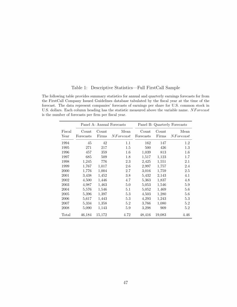
Table 1: Descriptive Statistics—Full FirstCall Sample
The following table provides summary statistics for annual and quarterly earnings forecasts for fromthe FirstCall Company Issued Guidelines database tabulated by the fiscal year at the time of theforecast. The data represent companies’ forecasts of earnings per share for U.S. common stock inU.S. dollars. Each column heading has the statistic measured above the variable name. NForecastis the number of forecasts per firm per fiscal year.
Panel A: Annual Forecasts Panel B: Quarterly Forecasts
Fiscal Count Count Mean Count Count MeanYear Forecasts Firms NForecast Forecasts Firms NForecast
1994 45 42 1.1 162 147 1.21995 271 217 1.5 500 426 1.31996 457 359 1.6 1,039 813 1.61997 685 509 1.8 1,517 1,123 1.71998 1,245 776 2.3 2,425 1,551 2.11999 1,767 1,017 2.6 2,997 1,757 2.42000 1,776 1,004 2.7 3,016 1,759 2.52001 3,438 1,452 3.8 5,432 2,143 4.12002 4,500 1,446 4.7 5,363 1,837 4.82003 4,987 1,463 5.0 5,053 1,546 5.92004 5,576 1,546 5.1 5,052 1,469 5.62005 5,396 1,397 5.3 4,503 1,280 5.62006 5,617 1,443 5.3 4,293 1,243 5.32007 5,334 1,358 5.2 3,766 1,080 5.22008 5,090 1,143 5.9 3,298 909 5.2
Total 46,184 15,172 4.72 48,416 19,083 4.46
47
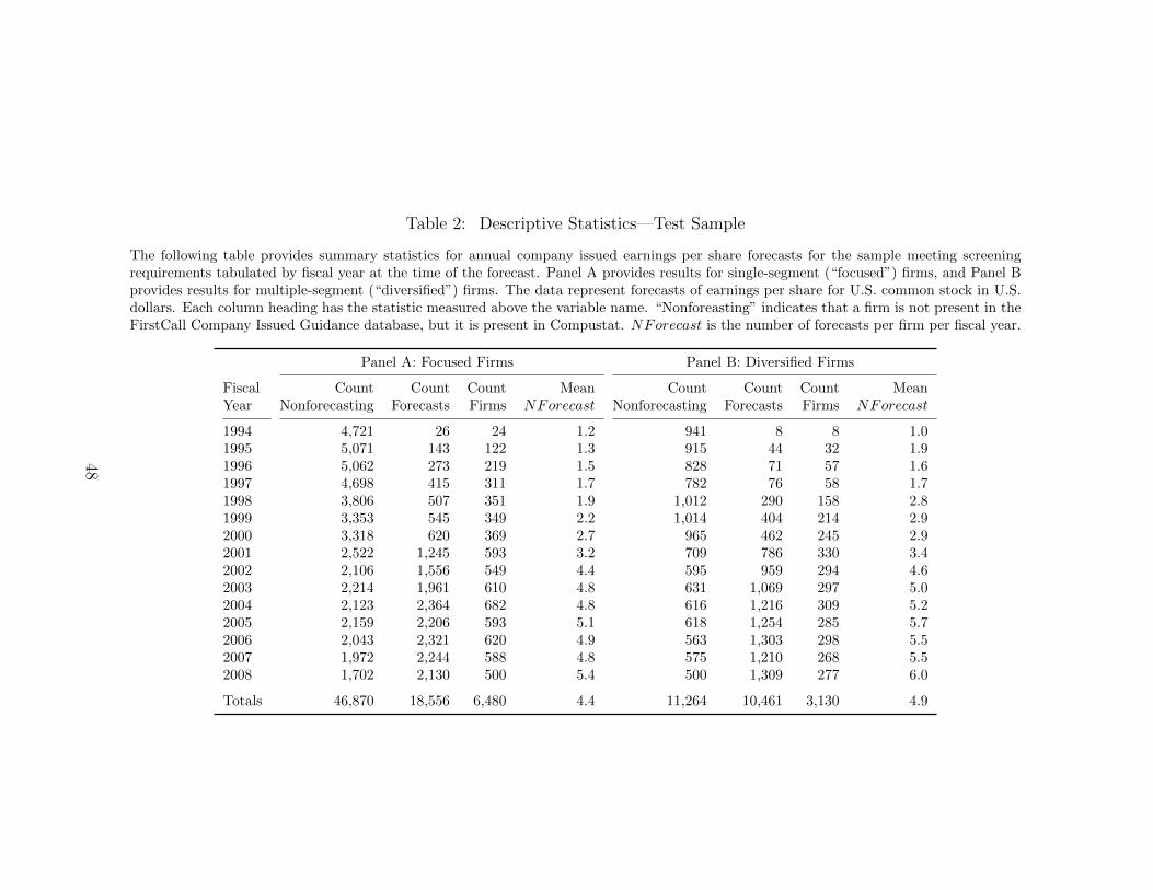
Table 2: Descriptive Statistics—Test Sample
The following table provides summary statistics for annual company issued earnings per share forecasts for the sample meeting screeningrequirements tabulated by fiscal year at the time of the forecast. Panel A provides results for single-segment (“focused”) firms, and Panel Bprovides results for multiple-segment (“diversified”) firms. The data represent forecasts of earnings per share for U.S. common stock in U.S.dollars. Each column heading has the statistic measured above the variable name. “Nonforeasting” indicates that a firm is not present in theFirstCall Company Issued Guidance database, but it is present in Compustat. NForecast is the number of forecasts per firm per fiscal year.
Panel A: Focused Firms Panel B: Diversified Firms
Fiscal Count Count Count Mean Count Count Count MeanYear Nonforecasting Forecasts Firms NForecast Nonforecasting Forecasts Firms NForecast
1994 4,721 26 24 1.2 941 8 8 1.01995 5,071 143 122 1.3 915 44 32 1.91996 5,062 273 219 1.5 828 71 57 1.61997 4,698 415 311 1.7 782 76 58 1.71998 3,806 507 351 1.9 1,012 290 158 2.81999 3,353 545 349 2.2 1,014 404 214 2.92000 3,318 620 369 2.7 965 462 245 2.92001 2,522 1,245 593 3.2 709 786 330 3.42002 2,106 1,556 549 4.4 595 959 294 4.62003 2,214 1,961 610 4.8 631 1,069 297 5.02004 2,123 2,364 682 4.8 616 1,216 309 5.22005 2,159 2,206 593 5.1 618 1,254 285 5.72006 2,043 2,321 620 4.9 563 1,303 298 5.52007 1,972 2,244 588 4.8 575 1,210 268 5.52008 1,702 2,130 500 5.4 500 1,309 277 6.0
Totals 46,870 18,556 6,480 4.4 11,264 10,461 3,130 4.9
48
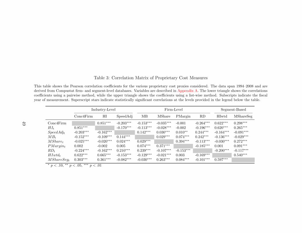
Table 3: Correlation Matrix of Proprietary Cost Measures
This table shows the Pearson correlation coefficients for the various proprietary cost proxies considered. The data span 1994–2008 and arederived from Compustat firm- and segment-level databases. Variables are described in Appendix A. The lower triangle shows the correlationscoefficients using a pairwise method, while the upper triangle shows the coefficients using a list-wise method. Subscripts indicate the fiscalyear of measurement. Superscript stars indicate statistically significant correlations at the levels provided in the legend below the table.
Industry-Level Firm-Level Segment-Based
Conc4Firm HI SpeedAdj MB MShare PMargin RD HIwtd MShareSeg
Conc4Firm 0.851∗∗∗ -0.203∗∗∗ -0.153∗∗∗ -0.035∗∗∗ -0.001 -0.264∗∗∗ 0.622∗∗∗ 0.298∗∗∗
HIt 0.851∗∗∗ -0.170∗∗∗ -0.113∗∗∗ -0.028∗∗∗ -0.002 -0.196∗∗∗ 0.620∗∗∗ 0.265∗∗∗
SpeedAdjt -0.203∗∗∗ -0.162∗∗∗ 0.142∗∗∗ 0.030∗∗∗ 0.010∗∗ 0.244∗∗∗ -0.164∗∗∗ -0.091∗∗∗
MBt -0.152∗∗∗ -0.109∗∗∗ 0.144∗∗∗ 0.029∗∗∗ 0.074∗∗∗ 0.242∗∗∗ -0.136∗∗∗ -0.029∗∗∗
MSharet -0.025∗∗∗ -0.020∗∗∗ 0.024∗∗∗ 0.029∗∗∗ 0.394∗∗∗ -0.113∗∗∗ -0.030∗∗∗ 0.272∗∗∗
PMargint 0.002 -0.002 0.005 0.074∗∗∗ 0.371∗∗∗ -0.185∗∗∗ 0.001 0.091∗∗∗
RDt -0.224∗∗∗ -0.162∗∗∗ 0.210∗∗∗ 0.239∗∗∗ -0.107∗∗∗ -0.153∗∗∗ -0.200∗∗∗ -0.117∗∗∗
HIwtdt 0.622∗∗∗ 0.665∗∗∗ -0.153∗∗∗ -0.129∗∗∗ -0.021∗∗∗ 0.003 -0.169∗∗∗ 0.540∗∗∗
MShareSegt 0.303∗∗∗ 0.361∗∗∗ -0.082∗∗∗ -0.030∗∗∗ 0.263∗∗∗ 0.084∗∗∗ -0.101∗∗∗ 0.597∗∗∗
∗ p < .10, ∗∗ p < .05, ∗∗∗ p < .01
49

Table 4: Forecasting Status Summary Statistics
This table presents statistics for variables of interest by forecasting status for the firm-level samplefor the fiscal years 1994–2008. A firm is considered “Nonforecasting” in a particular fiscal year if itis not represented in the FirstCall Company Issued Guidance database. For each of the variables inthe first column, the second and third columns contain the mean on the upper row and the standarddeviation on the lower row in parentheses. Variables are described in Appendix A. The “Diff.”column indicates the difference between Nonforecasting and Forecasting firm means, and asterisksindicate if the difference is significant at the 10% (*), 5% (**), or 1% (***) level. Subscripts indicatethe fiscal year of measurement.
Nonforecastingt Forecastingt
N N TotalMultit = 0 46,870 11,754 58,624Multit = 1 11,264 4,690 15,954
Mean/(sd) Mean/(sd) Diff. N
Multit 0.194 0.285 -0.091*** 74,578(0.395) (0.452)
Entropyt 0.120 0.179 -0.059*** 74,578(0.285) (0.334)
HIt 0.150 0.158 -0.008*** 74,578(0.137) (0.143)
SpeedAdjt 0.526 0.550 -0.024*** 74,351(0.313) (0.305)
PMargint 0.479 0.573 -0.094*** 68,345(0.306) (0.278)
RDt 0.066 0.052 0.014*** 74,555(0.193) (0.091)
HIwtdt 0.122 0.125 -0.003*** 74,578(0.132) (0.132)
MBt 0.797 0.796 0.001 65,465(1.120) (0.862)
EarnV olt 0.056 0.032 0.024*** 51,568(0.131) (0.075)
V olatilityt 0.165 0.142 0.023*** 44,666(0.107) (0.081)
Sizet 4.586 6.152 -1.565*** 74,555(2.235) (1.720)
NegEarnt 0.419 0.278 0.141*** 74,578(0.493) (0.448)
NegEarnGt 0.390 0.433 -0.043*** 74,578(0.488) (0.496)
ROEt -0.248 -0.043 -0.205*** 71,869(0.830) (0.541)
LitIndt 0.328 0.390 -0.062*** 74,578(0.461) (0.475)
NumEstt 3.469 6.212 -2.743*** 47,420(4.296) (5.723)
Dispersiont 0.108 0.066 0.042*** 33,984(0.215) (0.147)
50

Table 5: Forecast Issuance—Multi-segment
This table contains the coefficients from a logistic regression where the binary outcome is whether ornot a firm issued a management forecast in a given fiscal year. Data for management forecasts arederived from the FirstCall Company Issued Guidance database for the time period 1994–2008. Eachcolumn heading indicates the proprietary cost measure PC used in each model. Other variables aredescribed in Appendix A. The parentheses contain z-statistics adjusted for firm clustering.
HI SpeedAdj RD HIwtd MShareSeg
Multit 0.304∗∗∗ 0.283∗∗∗ 0.294∗∗∗ 0.305∗∗∗ 0.296∗∗∗ 0.306∗∗∗
(8.61) (8.19) (8.41) (8.75) (8.46) (8.52)PCt 0.977∗∗∗ 0.454∗∗∗ -1.117∗∗∗ 0.814∗∗∗ 1.130∗∗∗
(8.97) (7.96) (-2.93) (5.03) (5.18)MBt -0.104∗∗ -0.0984∗∗ -0.134∗∗∗ -0.0777 -0.0947∗∗ -0.113∗∗∗
(-2.41) (-2.25) (-3.17) (-1.57) (-2.16) (-2.64)EarnV olt 0.0439 0.0836 -0.00639 0.142 0.0819 0.0688
(0.14) (0.27) (-0.02) (0.43) (0.26) (0.22)V olatilityt 2.804∗∗ 2.980∗∗∗ 3.021∗∗∗ 2.846∗∗ 2.938∗∗ 2.934∗∗
(2.42) (2.59) (2.60) (2.43) (2.55) (2.56)Sizet 0.134∗∗∗ 0.128∗∗∗ 0.161∗∗∗ 0.118∗∗∗ 0.131∗∗∗ 0.106∗∗∗
(4.26) (4.05) (5.25) (3.68) (4.07) (3.05)NegEarnt -0.395∗∗∗ -0.379∗∗∗ -0.403∗∗∗ -0.358∗∗∗ -0.379∗∗∗ -0.388∗∗∗
(-4.83) (-4.67) (-4.90) (-4.66) (-4.73) (-4.79)NegEarnGt 0.356∗∗∗ 0.352∗∗∗ 0.351∗∗∗ 0.359∗∗∗ 0.356∗∗∗ 0.358∗∗∗
(4.36) (4.30) (4.32) (4.38) (4.35) (4.40)ROEt 0.156∗∗∗ 0.160∗∗∗ 0.163∗∗∗ 0.103∗∗∗ 0.160∗∗∗ 0.160∗∗∗
(3.38) (3.40) (3.44) (2.82) (3.42) (3.45)LitIndt 0.248∗∗∗ 0.299∗∗∗ 0.225∗∗∗ 0.310∗∗∗ 0.283∗∗∗ 0.273∗∗∗
(6.61) (6.51) (6.14) (6.13) (6.38) (6.48)NumEstt 0.0253∗∗∗ 0.0280∗∗∗ 0.0244∗∗∗ 0.0268∗∗∗ 0.0270∗∗∗ 0.0283∗∗∗
(3.71) (4.07) (3.66) (3.84) (3.84) (3.96)Dispersiont -1.511∗∗∗ -1.470∗∗∗ -1.513∗∗∗ -1.489∗∗∗ -1.486∗∗∗ -1.473∗∗∗
(-7.35) (-7.39) (-7.56) (-7.43) (-7.38) (-7.36)Constant -1.463∗∗∗ -1.640∗∗∗ -1.856∗∗∗ -1.378∗∗∗ -1.597∗∗∗ -1.394∗∗∗
(-3.34) (-3.77) (-4.32) (-3.10) (-3.68) (-3.10)
N 22694 22694 22629 22694 22694 22694Pseudo R2 0.0392 0.0421 0.0428 0.0405 0.0409 0.0423Log likelihood -15103.4 -15058.9 -15004.0 -15083.5 -15077.3 -15054.7∗ p < .10, ∗∗ p < .05, ∗∗∗ p < .01
51

Table 6: Forecast Issuance—Entropy
This table contains the coefficients from a logistic regression where the binary outcome is whether ornot a firm issued a management forecast in a given fiscal year. Data for management forecasts arederived from the FirstCall Company Issued Guidance database for the time period 1994–2008. Eachcolumn heading indicates the proprietary cost measure PC used in each model. Other variables aredescribed in Appendix A. The parentheses contain z-statistics adjusted for firm clustering.
HI SpeedAdj RD HIwtd MShareSeg
Entropyt 0.345∗∗∗ 0.310∗∗∗ 0.333∗∗∗ 0.353∗∗∗ 0.341∗∗∗ 0.354∗∗∗
(4.87) (4.37) (4.72) (5.05) (4.85) (4.96)PCt 0.979∗∗∗ 0.458∗∗∗ -1.152∗∗∗ 0.839∗∗∗ 1.141∗∗∗
(9.13) (8.00) (-3.01) (5.22) (5.25)MBt -0.109∗∗ -0.103∗∗ -0.139∗∗∗ -0.0816 -0.0990∗∗ -0.117∗∗∗
(-2.50) (-2.33) (-3.27) (-1.64) (-2.24) (-2.73)EarnV olt 0.0359 0.0768 -0.0146 0.136 0.0752 0.0607
(0.11) (0.25) (-0.05) (0.41) (0.24) (0.20)V olatilityt 2.844∗∗ 3.014∗∗∗ 3.062∗∗∗ 2.889∗∗ 2.981∗∗∗ 2.977∗∗∗
(2.46) (2.63) (2.64) (2.47) (2.60) (2.60)Sizet 0.136∗∗∗ 0.130∗∗∗ 0.162∗∗∗ 0.119∗∗∗ 0.132∗∗∗ 0.107∗∗∗
(4.08) (3.91) (5.00) (3.49) (3.88) (2.91)NegEarnt -0.399∗∗∗ -0.383∗∗∗ -0.406∗∗∗ -0.361∗∗∗ -0.382∗∗∗ -0.392∗∗∗
(-4.82) (-4.67) (-4.90) (-4.65) (-4.73) (-4.78)NegEarnGt 0.356∗∗∗ 0.352∗∗∗ 0.351∗∗∗ 0.358∗∗∗ 0.355∗∗∗ 0.358∗∗∗
(4.35) (4.28) (4.30) (4.37) (4.33) (4.39)ROEt 0.157∗∗∗ 0.160∗∗∗ 0.164∗∗∗ 0.102∗∗∗ 0.161∗∗∗ 0.161∗∗∗
(3.39) (3.42) (3.47) (2.80) (3.44) (3.47)LitIndt 0.237∗∗∗ 0.287∗∗∗ 0.214∗∗∗ 0.301∗∗∗ 0.273∗∗∗ 0.263∗∗∗
(6.03) (6.10) (5.52) (5.78) (5.93) (5.97)NumEstt 0.0252∗∗∗ 0.0278∗∗∗ 0.0243∗∗∗ 0.0268∗∗∗ 0.0270∗∗∗ 0.0283∗∗∗
(3.60) (3.94) (3.54) (3.74) (3.74) (3.85)Dispersiont -1.521∗∗∗ -1.480∗∗∗ -1.523∗∗∗ -1.498∗∗∗ -1.496∗∗∗ -1.483∗∗∗
(-7.43) (-7.46) (-7.64) (-7.51) (-7.45) (-7.43)Constant -1.445∗∗∗ -1.625∗∗∗ -1.841∗∗∗ -1.356∗∗∗ -1.582∗∗∗ -1.374∗∗∗
(-3.26) (-3.68) (-4.23) (-3.01) (-3.60) (-3.02)
N 22694 22694 22629 22694 22694 22694Pseudo R2 0.0384 0.0412 0.0420 0.0397 0.0402 0.0416Log likelihood -15116.5 -15072.0 -15016.2 -15095.4 -15088.7 -15066.6∗ p < .10, ∗∗ p < .05, ∗∗∗ p < .01
52

Table 7: Excess Value on Diversification and Disclosure Ranking
The following table presents results from an ordinary least squares regression with the dependentvariable of firm excess value as described in Appendix B. Each super-column heading indicates thedisclosure measure used in the various models. Disct indicates the percentile rank within three-digit SIC code industry of the yearly disclosure measure in the super-column. Firm fixed effects areincluded in each model. Other control variables are described in Appendix A. Data for managementforecasts are derived from the FirstCall Company Issued Guidance database over the period 1994–2008. Standard errors are clustered by firm, and resulting t-statistics are presented in parentheses.
NForecast Lead Spec Error abs(Error)
Multit -0.0750∗∗∗ -0.0326 -0.0310 -0.0571∗∗∗ -0.0654∗∗∗
(-3.52) (-1.62) (-1.39) (-2.73) (-3.04)Disct -0.00722 0.110∗∗∗ 0.107∗∗∗ -0.0206 -0.0952∗∗∗
(-0.28) (4.93) (4.26) (-0.84) (-3.84)MultiXDisct 0.126∗∗∗ 0.0298 0.0282 0.0796∗∗ 0.101∗∗∗
(2.99) (0.83) (0.67) (2.09) (2.64)Sizet 0.0457∗∗∗ 0.0440∗∗∗ 0.0467∗∗∗ 0.0429∗∗∗ 0.0414∗∗∗
(8.75) (8.45) (9.02) (7.67) (7.40)Investt 0.467∗∗∗ 0.460∗∗∗ 0.467∗∗∗ 0.501∗∗∗ 0.499∗∗∗
(9.61) (9.48) (9.58) (8.36) (8.31)EBITt -0.0244∗∗∗ -0.0242∗∗∗ -0.0244∗∗∗ -0.0155 -0.0183
(-3.11) (-3.11) (-3.11) (-1.34) (-1.60)Leveraget -0.202∗∗∗ -0.186∗∗∗ -0.197∗∗∗ -0.218∗∗∗ -0.222∗∗∗
(-4.59) (-4.26) (-4.49) (-4.63) (-4.72)Constant -0.262∗∗∗ -0.303∗∗∗ -0.317∗∗∗ -0.234∗∗∗ -0.193∗∗∗
(-8.64) (-9.91) (-10.35) (-6.78) (-5.56)
N 13674 13674 13671 11678 11678Adj. R2 0.0441 0.0473 0.0457 0.0371 0.0386∗ p < .10, ∗∗ p < .05, ∗∗∗ p < .01
53
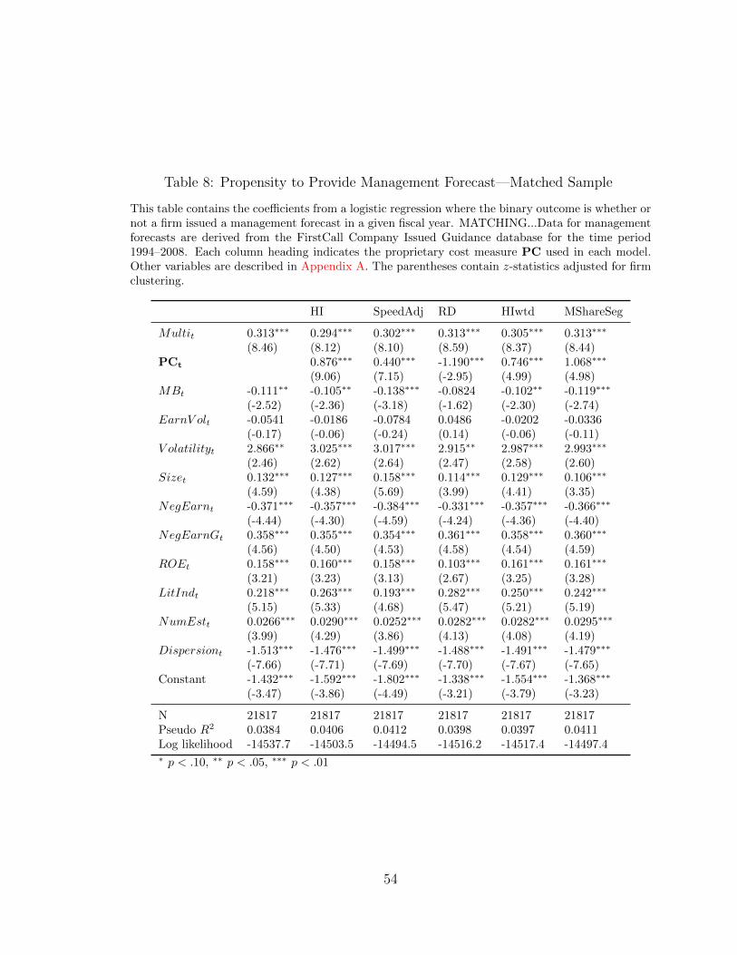
Table 8: Propensity to Provide Management Forecast—Matched Sample
This table contains the coefficients from a logistic regression where the binary outcome is whether ornot a firm issued a management forecast in a given fiscal year. MATCHING...Data for managementforecasts are derived from the FirstCall Company Issued Guidance database for the time period1994–2008. Each column heading indicates the proprietary cost measure PC used in each model.Other variables are described in Appendix A. The parentheses contain z-statistics adjusted for firmclustering.
HI SpeedAdj RD HIwtd MShareSeg
Multit 0.313∗∗∗ 0.294∗∗∗ 0.302∗∗∗ 0.313∗∗∗ 0.305∗∗∗ 0.313∗∗∗
(8.46) (8.12) (8.10) (8.59) (8.37) (8.44)PCt 0.876∗∗∗ 0.440∗∗∗ -1.190∗∗∗ 0.746∗∗∗ 1.068∗∗∗
(9.06) (7.15) (-2.95) (4.99) (4.98)MBt -0.111∗∗ -0.105∗∗ -0.138∗∗∗ -0.0824 -0.102∗∗ -0.119∗∗∗
(-2.52) (-2.36) (-3.18) (-1.62) (-2.30) (-2.74)EarnV olt -0.0541 -0.0186 -0.0784 0.0486 -0.0202 -0.0336
(-0.17) (-0.06) (-0.24) (0.14) (-0.06) (-0.11)V olatilityt 2.866∗∗ 3.025∗∗∗ 3.017∗∗∗ 2.915∗∗ 2.987∗∗∗ 2.993∗∗∗
(2.46) (2.62) (2.64) (2.47) (2.58) (2.60)Sizet 0.132∗∗∗ 0.127∗∗∗ 0.158∗∗∗ 0.114∗∗∗ 0.129∗∗∗ 0.106∗∗∗
(4.59) (4.38) (5.69) (3.99) (4.41) (3.35)NegEarnt -0.371∗∗∗ -0.357∗∗∗ -0.384∗∗∗ -0.331∗∗∗ -0.357∗∗∗ -0.366∗∗∗
(-4.44) (-4.30) (-4.59) (-4.24) (-4.36) (-4.40)NegEarnGt 0.358∗∗∗ 0.355∗∗∗ 0.354∗∗∗ 0.361∗∗∗ 0.358∗∗∗ 0.360∗∗∗
(4.56) (4.50) (4.53) (4.58) (4.54) (4.59)ROEt 0.158∗∗∗ 0.160∗∗∗ 0.158∗∗∗ 0.103∗∗∗ 0.161∗∗∗ 0.161∗∗∗
(3.21) (3.23) (3.13) (2.67) (3.25) (3.28)LitIndt 0.218∗∗∗ 0.263∗∗∗ 0.193∗∗∗ 0.282∗∗∗ 0.250∗∗∗ 0.242∗∗∗
(5.15) (5.33) (4.68) (5.47) (5.21) (5.19)NumEstt 0.0266∗∗∗ 0.0290∗∗∗ 0.0252∗∗∗ 0.0282∗∗∗ 0.0282∗∗∗ 0.0295∗∗∗
(3.99) (4.29) (3.86) (4.13) (4.08) (4.19)Dispersiont -1.513∗∗∗ -1.476∗∗∗ -1.499∗∗∗ -1.488∗∗∗ -1.491∗∗∗ -1.479∗∗∗
(-7.66) (-7.71) (-7.69) (-7.70) (-7.67) (-7.65)Constant -1.432∗∗∗ -1.592∗∗∗ -1.802∗∗∗ -1.338∗∗∗ -1.554∗∗∗ -1.368∗∗∗
(-3.47) (-3.86) (-4.49) (-3.21) (-3.79) (-3.23)
N 21817 21817 21817 21817 21817 21817Pseudo R2 0.0384 0.0406 0.0412 0.0398 0.0397 0.0411Log likelihood -14537.7 -14503.5 -14494.5 -14516.2 -14517.4 -14497.4∗ p < .10, ∗∗ p < .05, ∗∗∗ p < .01
54
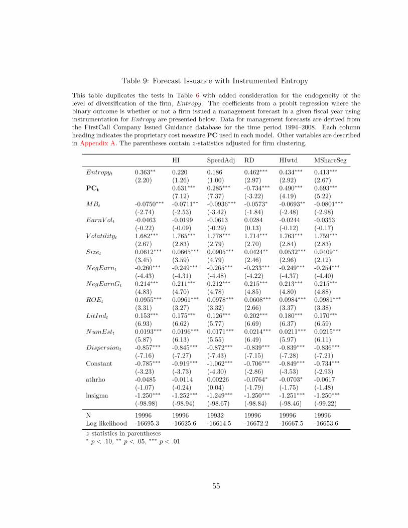
Table 9: Forecast Issuance with Instrumented Entropy
This table duplicates the tests in Table 6 with added consideration for the endogeneity of thelevel of diversification of the firm, Entropy. The coefficients from a probit regression where thebinary outcome is whether or not a firm issued a management forecast in a given fiscal year usinginstrumentation for Entropy are presented below. Data for management forecasts are derived fromthe FirstCall Company Issued Guidance database for the time period 1994–2008. Each columnheading indicates the proprietary cost measure PC used in each model. Other variables are describedin Appendix A. The parentheses contain z-statistics adjusted for firm clustering.
HI SpeedAdj RD HIwtd MShareSeg
Entropyt 0.363∗∗ 0.220 0.186 0.462∗∗∗ 0.434∗∗∗ 0.413∗∗∗
(2.20) (1.26) (1.00) (2.97) (2.92) (2.67)PCt 0.631∗∗∗ 0.285∗∗∗ -0.734∗∗∗ 0.490∗∗∗ 0.693∗∗∗
(7.12) (7.37) (-3.22) (4.19) (5.22)MBt -0.0750∗∗∗ -0.0711∗∗ -0.0936∗∗∗ -0.0573∗ -0.0693∗∗ -0.0801∗∗∗
(-2.74) (-2.53) (-3.42) (-1.84) (-2.48) (-2.98)EarnV olt -0.0463 -0.0199 -0.0613 0.0284 -0.0244 -0.0353
(-0.22) (-0.09) (-0.29) (0.13) (-0.12) (-0.17)V olatilityt 1.682∗∗∗ 1.765∗∗∗ 1.778∗∗∗ 1.714∗∗∗ 1.763∗∗∗ 1.759∗∗∗
(2.67) (2.83) (2.79) (2.70) (2.84) (2.83)Sizet 0.0612∗∗∗ 0.0665∗∗∗ 0.0905∗∗∗ 0.0424∗∗ 0.0532∗∗∗ 0.0409∗∗
(3.45) (3.59) (4.79) (2.46) (2.96) (2.12)NegEarnt -0.260∗∗∗ -0.249∗∗∗ -0.265∗∗∗ -0.233∗∗∗ -0.249∗∗∗ -0.254∗∗∗
(-4.43) (-4.31) (-4.48) (-4.22) (-4.37) (-4.40)NegEarnGt 0.214∗∗∗ 0.211∗∗∗ 0.212∗∗∗ 0.215∗∗∗ 0.213∗∗∗ 0.215∗∗∗
(4.83) (4.70) (4.78) (4.85) (4.80) (4.88)ROEt 0.0955∗∗∗ 0.0961∗∗∗ 0.0978∗∗∗ 0.0608∗∗∗ 0.0984∗∗∗ 0.0981∗∗∗
(3.31) (3.27) (3.32) (2.66) (3.37) (3.38)LitIndt 0.153∗∗∗ 0.175∗∗∗ 0.126∗∗∗ 0.202∗∗∗ 0.180∗∗∗ 0.170∗∗∗
(6.93) (6.62) (5.77) (6.69) (6.37) (6.59)NumEstt 0.0193∗∗∗ 0.0196∗∗∗ 0.0171∗∗∗ 0.0214∗∗∗ 0.0211∗∗∗ 0.0215∗∗∗
(5.87) (6.13) (5.55) (6.49) (5.97) (6.11)Dispersiont -0.857∗∗∗ -0.845∗∗∗ -0.872∗∗∗ -0.839∗∗∗ -0.839∗∗∗ -0.836∗∗∗
(-7.16) (-7.27) (-7.43) (-7.15) (-7.28) (-7.21)Constant -0.785∗∗∗ -0.919∗∗∗ -1.062∗∗∗ -0.706∗∗∗ -0.849∗∗∗ -0.734∗∗∗
(-3.23) (-3.73) (-4.30) (-2.86) (-3.53) (-2.93)athrho -0.0485 -0.0114 0.00226 -0.0764∗ -0.0703∗ -0.0617
(-1.07) (-0.24) (0.04) (-1.79) (-1.75) (-1.48)lnsigma -1.250∗∗∗ -1.252∗∗∗ -1.249∗∗∗ -1.250∗∗∗ -1.251∗∗∗ -1.250∗∗∗
(-98.98) (-98.94) (-98.67) (-98.84) (-98.46) (-99.22)
N 19996 19996 19932 19996 19996 19996Log likelihood -16695.3 -16625.6 -16614.5 -16672.2 -16667.5 -16653.6
z statistics in parentheses∗ p < .10, ∗∗ p < .05, ∗∗∗ p < .01
55

Table 10: Forecast Issuance—Regulation Fair Disclosure
This table duplicates the tests in Table 5 with an additional control for forecasts occurring afterRegFD. RegFD is a dummy variable indicating the period after Reg FD. An “X” between variablenames indicates an interaction term. The control variables from Table 5 have been included whenidentification is possible, but their coefficients are not shown for brevity.
HI SpeedAdj RD HIwtd MShareSeg
Multit 0.171 0.157 0.162 0.179 0.169 0.174(1.56) (1.43) (1.47) (1.64) (1.54) (1.56)
PCt 0.764∗∗∗ 0.385∗∗∗ -1.231∗∗∗ 0.665∗∗∗ 1.155∗∗∗
(5.70) (5.93) (-3.17) (3.61) (5.11)RegFD 0.791∗∗∗ 0.776∗∗∗ 0.779∗∗∗ 0.799∗∗∗ 0.785∗∗∗ 0.793∗∗∗
(3.09) (3.03) (3.04) (3.11) (3.06) (3.07)MultiXRegFD 0.176 0.171 0.177 0.165 0.169 0.174
(1.48) (1.43) (1.50) (1.40) (1.43) (1.44)MBt -0.0827∗ -0.0783 -0.109∗∗ -0.0532 -0.0750 -0.0908∗
(-1.68) (-1.58) (-2.18) (-0.98) (-1.51) (-1.86)EarnV olt 0.111 0.142 0.0682 0.211 0.143 0.137
(0.31) (0.40) (0.18) (0.56) (0.40) (0.38)V olatilityt 1.807∗∗∗ 1.959∗∗∗ 1.998∗∗∗ 1.845∗∗∗ 1.921∗∗∗ 1.934∗∗∗
(2.96) (3.25) (3.22) (3.00) (3.21) (3.22)Sizet 0.0992∗∗∗ 0.0949∗∗∗ 0.122∗∗∗ 0.0811∗∗∗ 0.0966∗∗∗ 0.0703∗∗∗
(5.14) (4.84) (6.83) (4.03) (4.85) (3.12)NegEarnt -0.444∗∗∗ -0.430∗∗∗ -0.448∗∗∗ -0.404∗∗∗ -0.430∗∗∗ -0.437∗∗∗
(-5.10) (-5.03) (-5.09) (-4.94) (-5.09) (-5.06)NegEarnGt 0.368∗∗∗ 0.365∗∗∗ 0.363∗∗∗ 0.370∗∗∗ 0.367∗∗∗ 0.370∗∗∗
(4.68) (4.61) (4.66) (4.70) (4.66) (4.73)ROEt 0.195∗∗∗ 0.197∗∗∗ 0.201∗∗∗ 0.134∗∗∗ 0.197∗∗∗ 0.199∗∗∗
(3.89) (3.90) (3.97) (3.20) (3.92) (3.96)LitIndt 0.237∗∗∗ 0.276∗∗∗ 0.219∗∗∗ 0.305∗∗∗ 0.265∗∗∗ 0.261∗∗∗
(6.55) (6.27) (6.31) (6.14) (6.19) (6.44)NumEstt 0.0224∗∗∗ 0.0246∗∗∗ 0.0218∗∗∗ 0.0241∗∗∗ 0.0238∗∗∗ 0.0254∗∗∗
(3.49) (3.73) (3.49) (3.63) (3.55) (3.73)Dispersiont -1.536∗∗∗ -1.502∗∗∗ -1.539∗∗∗ -1.511∗∗∗ -1.515∗∗∗ -1.496∗∗∗
(-6.28) (-6.35) (-6.50) (-6.33) (-6.32) (-6.27)Constant -1.604∗∗∗ -1.738∗∗∗ -1.935∗∗∗ -1.511∗∗∗ -1.711∗∗∗ -1.533∗∗∗
(-4.53) (-4.92) (-5.55) (-4.33) (-4.85) (-4.24)
N 22693 22693 22628 22693 22693 22693Pseudo R2 0.0651 0.0667 0.0678 0.0666 0.0661 0.0682Log likelihood -14696.4 -14670.2 -14611.1 -14673.1 -14679.6 -14648.0
z statistics in parentheses∗ p < .10, ∗∗ p < .05, ∗∗∗ p < .01
56

Table 11: Summary Statistics by Periodicity and Diversification Status
This table presents statistics for more granular measures of management forecasts using aforecast-level sample for fiscal years 1994–2008. The left panel of the table shows statistics forquarterly earnings forecasts, while the right panel shows statistics for annual earnings forecasts.Variables are described in Appendix A. Each panel is further divided by diversification status. Afirm is considered “focused” if it reports only one business segment and “diversified” if it reportsmore than one business segment. For each variable by periodicity and diversification status, themean is on the upper row and the standard deviation on the lower row in parentheses. The “Diff.”column indicates the difference between Focused and Diversified firm means, and asterisks indicateif the difference is significant at the 10% (*), 5% (**), or 1% (***) level. Subscripts indicate thefiscal year of measurement.
Quarterly Annual
Focusedt Diversifiedt Focusedt Diversifiedt
Mean/(sd) Mean/(sd) Diff. N Mean/(sd) Mean/(sd) Diff. N
NForecastt 6.725 7.961 -1.236*** 35,668 7.368 7.984 -0.616*** 29,015(5.482) (6.776) (4.875) (5.373)
Leadt 49.249 50.980 -1.731** 35,668 210.538 211.300 -0.762 29,015(64.580) (62.016) (135.078) (134.251)
Spect 2.986 2.963 0.023*** 35,661 3.052 3.045 0.006 29,013(0.779) (0.736) (0.626) (0.559)
Errort 0.354 0.270 0.084*** 31,718 1.131 1.086 0.045 26,993(2.297) (1.886) (3.253) (3.039)
|Errort| 0.751 0.637 0.114*** 31,718 1.752 1.720 0.032 26,993(2.199) (1.795) (2.966) (2.731)
HIt 0.146 0.185 -0.039*** 35,668 0.173 0.209 -0.036*** 29,015(0.133) (0.148) (0.161) (0.173)
SpeedAdjt 0.547 0.515 0.032*** 35,606 0.602 0.541 0.060*** 28,984(0.296) (0.291) (0.306) (0.304)
(Table continues on the next page.)
57
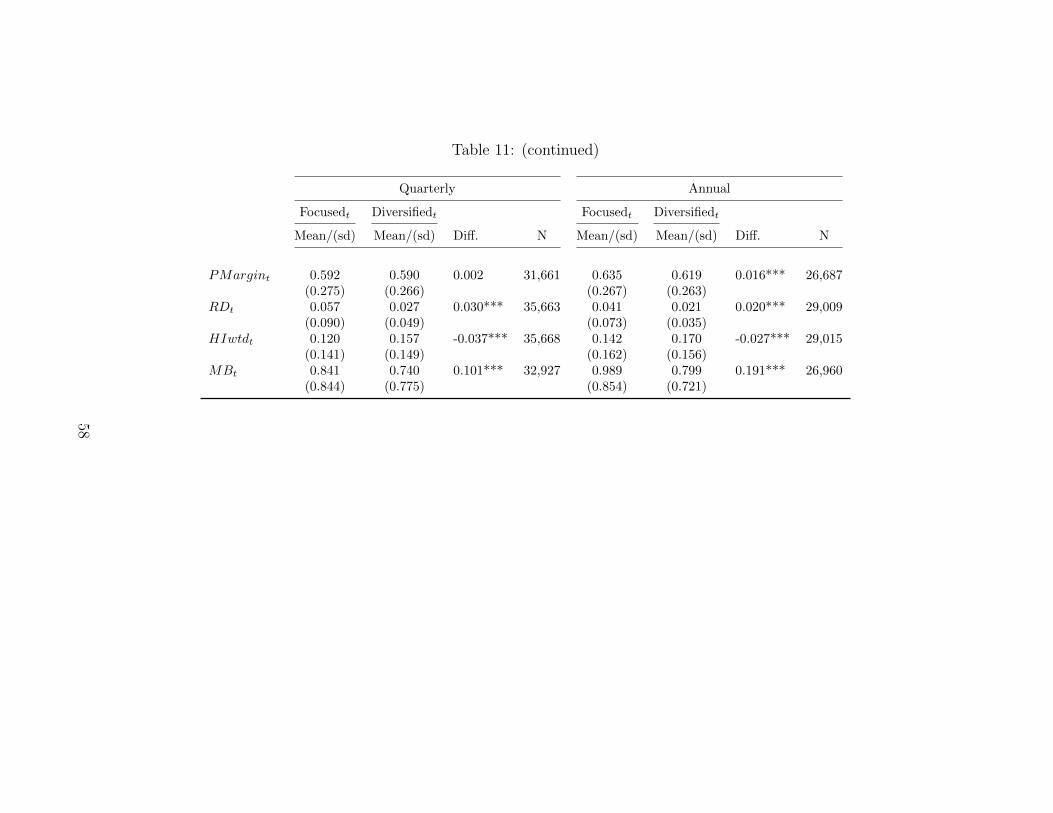
Table 11: (continued)
Quarterly Annual
Focusedt Diversifiedt Focusedt Diversifiedt
Mean/(sd) Mean/(sd) Diff. N Mean/(sd) Mean/(sd) Diff. N
PMargint 0.592 0.590 0.002 31,661 0.635 0.619 0.016*** 26,687(0.275) (0.266) (0.267) (0.263)
RDt 0.057 0.027 0.030*** 35,663 0.041 0.021 0.020*** 29,009(0.090) (0.049) (0.073) (0.035)
HIwtdt 0.120 0.157 -0.037*** 35,668 0.142 0.170 -0.027*** 29,015(0.141) (0.149) (0.162) (0.156)
MBt 0.841 0.740 0.101*** 32,927 0.989 0.799 0.191*** 26,960(0.844) (0.775) (0.854) (0.721)
58

Table 12: Forecast Lead—Multi-segment
The following table presents results from an ordinary least squares regression of the lead time of a forecast (Lead) on the multi-segment indicator (Multi) and othercontrol variables for the period 1994–2008. Other variables are described in Appendix A. Data for management forecasts are derived from the FirstCall CompanyIssued Guidance database. Each super-column heading indicates the periodicity of the forecasts and each column heading indicates the proprietary cost measure PCused in each model. All models include firm fixed effects. Standard errors are clustered by firm with t-statistics in parentheses.
Annual Forecasts Quarterly Forecasts
HI PMargin RD HIwtd MShareSeg HI PMargin RD HIwtd MShareSeg
Multit -2.841 -2.820 -2.857 -2.824 -2.809 -2.550 2.167 2.122 2.219 2.159 2.232 2.220(-0.53) (-0.53) (-0.53) (-0.53) (-0.52) (-0.47) (0.69) (0.68) (0.71) (0.69) (0.70) (0.72)
PCt -9.886 6.231 -13.42 -3.782 17.52 22.44∗ 4.190 1.519 -7.467 9.657(-0.50) (0.33) (-0.26) (-0.19) (0.80) (1.78) (0.35) (0.03) (-0.71) (0.65)
MBt 6.437∗∗ 6.350∗∗ 6.559∗∗ 6.475∗∗ 6.430∗∗ 6.397∗∗ 3.662∗∗∗ 3.710∗∗∗ 3.658∗∗∗ 3.659∗∗∗ 3.689∗∗∗ 3.622∗∗∗
(2.19) (2.15) (2.24) (2.19) (2.19) (2.18) (3.01) (3.05) (3.00) (2.96) (3.06) (2.95)EarnV olt -31.94∗ -31.97∗ -31.88∗ -31.13∗ -32.03∗ -31.70∗ -13.18 -12.90 -12.93 -13.23 -13.24 -13.15
(-1.91) (-1.90) (-1.90) (-1.86) (-1.91) (-1.89) (-1.15) (-1.12) (-1.11) (-1.17) (-1.16) (-1.15)V olatilityt 245.5∗∗∗ 245.4∗∗∗ 245.9∗∗∗ 245.0∗∗∗ 245.0∗∗∗ 247.3∗∗∗ 25.28∗ 25.25∗ 25.62∗ 25.38∗ 24.43∗ 26.06∗
(7.41) (7.42) (7.42) (7.38) (7.34) (7.46) (1.68) (1.69) (1.70) (1.68) (1.66) (1.67)Sizet 11.33∗∗ 11.50∗∗ 11.52∗∗ 11.16∗∗ 11.40∗∗ 11.08∗∗ 17.32∗∗∗ 17.06∗∗∗ 17.18∗∗∗ 17.35∗∗∗ 17.43∗∗∗ 17.22∗∗∗
(2.44) (2.48) (2.47) (2.38) (2.47) (2.40) (9.09) (8.99) (9.02) (8.52) (9.16) (9.01)NegEarnt 3.935 4.039 3.829 4.097 3.993 3.772 -4.141∗∗ -4.214∗∗ -4.262∗∗ -4.155∗∗ -4.082∗∗ -4.163∗∗
(0.83) (0.85) (0.81) (0.85) (0.85) (0.80) (-2.07) (-2.10) (-2.12) (-2.11) (-2.04) (-2.07)NegEarnGt 0.615 0.577 0.629 0.664 0.596 0.634 -0.383 -0.346 -0.280 -0.386 -0.424 -0.363
(0.30) (0.28) (0.31) (0.33) (0.29) (0.31) (-0.30) (-0.27) (-0.22) (-0.31) (-0.34) (-0.29)ROEt -1.536 -1.513 -1.696 -1.600 -1.514 -1.723 6.018∗∗∗ 6.128∗∗∗ 6.067∗∗∗ 6.038∗∗∗ 6.023∗∗∗ 5.993∗∗∗
(-0.27) (-0.26) (-0.29) (-0.28) (-0.26) (-0.30) (3.15) (3.20) (3.16) (2.96) (3.15) (3.14)LitIndt 36.23∗∗ 35.22∗∗ 36.12∗∗ 36.23∗∗ 36.05∗∗ 36.72∗∗ 14.53∗ 16.84∗∗ 14.28∗ 14.53∗ 14.34∗ 14.63∗
(2.08) (1.99) (2.08) (2.07) (2.07) (2.11) (1.72) (2.00) (1.69) (1.72) (1.70) (1.73)NumEstt -2.489∗∗∗ -2.488∗∗∗ -2.514∗∗∗ -2.484∗∗∗ -2.487∗∗∗ -2.494∗∗∗ -2.928∗∗∗ -2.933∗∗∗ -2.907∗∗∗ -2.928∗∗∗ -2.923∗∗∗ -2.932∗∗∗
(-3.96) (-3.95) (-3.98) (-3.97) (-3.95) (-3.97) (-9.77) (-9.76) (-9.69) (-9.90) (-9.76) (-9.75)Dispersiont 388.7∗∗∗ 388.9∗∗∗ 388.6∗∗∗ 388.7∗∗∗ 388.8∗∗∗ 388.5∗∗∗ 131.6∗∗∗ 131.2∗∗∗ 131.6∗∗∗ 131.6∗∗∗ 131.8∗∗∗ 131.5∗∗∗
(8.11) (8.10) (8.10) (8.10) (8.10) (8.10) (4.85) (4.86) (4.85) (4.86) (4.85) (4.85)Constant 84.12∗∗ 85.17∗∗ 79.21∗∗ 85.66∗∗ 84.31∗∗ 83.75∗∗ -58.69∗∗∗ -61.52∗∗∗ -60.07∗∗∗ -58.98∗∗∗ -58.34∗∗∗ -58.91∗∗∗
(2.51) (2.51) (2.34) (2.51) (2.50) (2.50) (-4.36) (-4.52) (-3.99) (-3.77) (-4.32) (-4.37)
N 20569 20569 20548 20569 20569 20569 23353 23353 23324 23353 23353 23353Adj. R2 0.118 0.118 0.118 0.118 0.118 0.118 0.317 0.317 0.318 0.317 0.317 0.317∗ p < .10, ∗∗ p < .05, ∗∗∗ p < .01
59
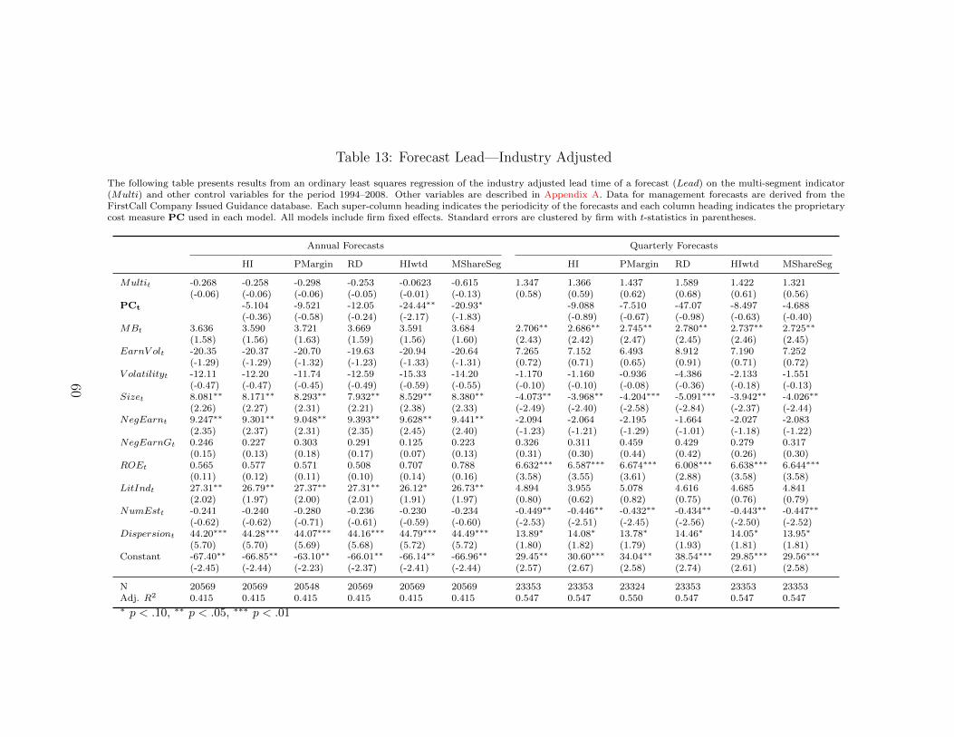
Table 13: Forecast Lead—Industry Adjusted
The following table presents results from an ordinary least squares regression of the industry adjusted lead time of a forecast (Lead) on the multi-segment indicator(Multi) and other control variables for the period 1994–2008. Other variables are described in Appendix A. Data for management forecasts are derived from theFirstCall Company Issued Guidance database. Each super-column heading indicates the periodicity of the forecasts and each column heading indicates the proprietarycost measure PC used in each model. All models include firm fixed effects. Standard errors are clustered by firm with t-statistics in parentheses.
Annual Forecasts Quarterly Forecasts
HI PMargin RD HIwtd MShareSeg HI PMargin RD HIwtd MShareSeg
Multit -0.268 -0.258 -0.298 -0.253 -0.0623 -0.615 1.347 1.366 1.437 1.589 1.422 1.321(-0.06) (-0.06) (-0.06) (-0.05) (-0.01) (-0.13) (0.58) (0.59) (0.62) (0.68) (0.61) (0.56)
PCt -5.104 -9.521 -12.05 -24.44∗∗ -20.93∗ -9.088 -7.510 -47.07 -8.497 -4.688(-0.36) (-0.58) (-0.24) (-2.17) (-1.83) (-0.89) (-0.67) (-0.98) (-0.63) (-0.40)
MBt 3.636 3.590 3.721 3.669 3.591 3.684 2.706∗∗ 2.686∗∗ 2.745∗∗ 2.780∗∗ 2.737∗∗ 2.725∗∗
(1.58) (1.56) (1.63) (1.59) (1.56) (1.60) (2.43) (2.42) (2.47) (2.45) (2.46) (2.45)EarnV olt -20.35 -20.37 -20.70 -19.63 -20.94 -20.64 7.265 7.152 6.493 8.912 7.190 7.252
(-1.29) (-1.29) (-1.32) (-1.23) (-1.33) (-1.31) (0.72) (0.71) (0.65) (0.91) (0.71) (0.72)V olatilityt -12.11 -12.20 -11.74 -12.59 -15.33 -14.20 -1.170 -1.160 -0.936 -4.386 -2.133 -1.551
(-0.47) (-0.47) (-0.45) (-0.49) (-0.59) (-0.55) (-0.10) (-0.10) (-0.08) (-0.36) (-0.18) (-0.13)Sizet 8.081∗∗ 8.171∗∗ 8.293∗∗ 7.932∗∗ 8.529∗∗ 8.380∗∗ -4.073∗∗ -3.968∗∗ -4.204∗∗∗ -5.091∗∗∗ -3.942∗∗ -4.026∗∗
(2.26) (2.27) (2.31) (2.21) (2.38) (2.33) (-2.49) (-2.40) (-2.58) (-2.84) (-2.37) (-2.44)NegEarnt 9.247∗∗ 9.301∗∗ 9.048∗∗ 9.393∗∗ 9.628∗∗ 9.441∗∗ -2.094 -2.064 -2.195 -1.664 -2.027 -2.083
(2.35) (2.37) (2.31) (2.35) (2.45) (2.40) (-1.23) (-1.21) (-1.29) (-1.01) (-1.18) (-1.22)NegEarnGt 0.246 0.227 0.303 0.291 0.125 0.223 0.326 0.311 0.459 0.429 0.279 0.317
(0.15) (0.13) (0.18) (0.17) (0.07) (0.13) (0.31) (0.30) (0.44) (0.42) (0.26) (0.30)ROEt 0.565 0.577 0.571 0.508 0.707 0.788 6.632∗∗∗ 6.587∗∗∗ 6.674∗∗∗ 6.008∗∗∗ 6.638∗∗∗ 6.644∗∗∗
(0.11) (0.12) (0.11) (0.10) (0.14) (0.16) (3.58) (3.55) (3.61) (2.88) (3.58) (3.58)LitIndt 27.31∗∗ 26.79∗∗ 27.37∗∗ 27.31∗∗ 26.12∗ 26.73∗∗ 4.894 3.955 5.078 4.616 4.685 4.841
(2.02) (1.97) (2.00) (2.01) (1.91) (1.97) (0.80) (0.62) (0.82) (0.75) (0.76) (0.79)NumEstt -0.241 -0.240 -0.280 -0.236 -0.230 -0.234 -0.449∗∗ -0.446∗∗ -0.432∗∗ -0.434∗∗ -0.443∗∗ -0.447∗∗
(-0.62) (-0.62) (-0.71) (-0.61) (-0.59) (-0.60) (-2.53) (-2.51) (-2.45) (-2.56) (-2.50) (-2.52)Dispersiont 44.20∗∗∗ 44.28∗∗∗ 44.07∗∗∗ 44.16∗∗∗ 44.79∗∗∗ 44.49∗∗∗ 13.89∗ 14.08∗ 13.78∗ 14.46∗ 14.05∗ 13.95∗
(5.70) (5.70) (5.69) (5.68) (5.72) (5.72) (1.80) (1.82) (1.79) (1.93) (1.81) (1.81)Constant -67.40∗∗ -66.85∗∗ -63.10∗∗ -66.01∗∗ -66.14∗∗ -66.96∗∗ 29.45∗∗ 30.60∗∗∗ 34.04∗∗ 38.54∗∗∗ 29.85∗∗∗ 29.56∗∗∗
(-2.45) (-2.44) (-2.23) (-2.37) (-2.41) (-2.44) (2.57) (2.67) (2.58) (2.74) (2.61) (2.58)
N 20569 20569 20548 20569 20569 20569 23353 23353 23324 23353 23353 23353Adj. R2 0.415 0.415 0.415 0.415 0.415 0.415 0.547 0.547 0.550 0.547 0.547 0.547∗ p < .10, ∗∗ p < .05, ∗∗∗ p < .01
60

Table 14: Specificity—Forecast Level
The following table presents results from an ordered probit regression of the specificity of a forecast (Spec) on the multi-segment indicator (Multi) and other controlvariables for the period 1994–2008. Other variables are described in Appendix A. Data for management forecasts are derived from the FirstCall Company IssuedGuidance database. Each super-column heading indicates the periodicity of the forecasts and each column heading indicates the proprietary cost measure PC usedin each model. The parentheses contain z-statistics.
Annual Forecasts Quarterly Forecasts
HI PMargin RD HIwtd MShareSeg HI PMargin RD HIwtd MShareSeg
Multit -0.0264 -0.0265 -0.0265 -0.0260 -0.0262 -0.0286 -0.0878∗∗ -0.0907∗∗∗ -0.0881∗∗ -0.0895∗∗ -0.0887∗∗ -0.0875∗∗
(-0.69) (-0.70) (-0.70) (-0.69) (-0.69) (-0.76) (-2.52) (-2.60) (-2.53) (-2.56) (-2.54) (-2.51)PCt 0.0123 0.00604 0.297 -0.148∗ -0.184∗∗ 0.232∗∗ 0.0346 -0.695∗∗∗ 0.0613 -0.0150
(0.12) (0.09) (0.86) (-1.70) (-2.39) (2.30) (0.63) (-2.85) (0.64) (-0.17)MBt 0.0178 0.0180 0.0174 0.0119 0.0149 0.0184 0.0418∗ 0.0433∗∗ 0.0395∗ 0.0561∗∗ 0.0427∗∗ 0.0418∗
(0.69) (0.70) (0.67) (0.44) (0.58) (0.72) (1.94) (2.02) (1.79) (2.49) (1.98) (1.94)EarnV olt 1.385∗∗∗ 1.386∗∗∗ 1.384∗∗∗ 1.357∗∗∗ 1.373∗∗∗ 1.373∗∗∗ 0.0615 0.0649 0.0636 0.0944 0.0617 0.0612
(3.59) (3.60) (3.62) (3.45) (3.57) (3.57) (0.31) (0.32) (0.32) (0.47) (0.31) (0.30)V olatilityt -0.219 -0.217 -0.209 -0.227 -0.247 -0.247 -0.568∗∗ -0.520∗∗ -0.550∗∗ -0.506∗ -0.555∗∗ -0.569∗∗
(-0.64) (-0.63) (-0.61) (-0.67) (-0.72) (-0.72) (-2.17) (-1.98) (-2.10) (-1.96) (-2.10) (-2.17)Sizet -0.0266 -0.0267 -0.0263 -0.0248 -0.0258 -0.0208 -0.0127 -0.0146 -0.0105 -0.0185 -0.0129 -0.0123
(-1.56) (-1.55) (-1.51) (-1.45) (-1.51) (-1.21) (-0.89) (-1.01) (-0.73) (-1.27) (-0.90) (-0.85)NegEarnt -0.0680 -0.0680 -0.0679 -0.0770 -0.0704 -0.0695 -0.110∗∗∗ -0.105∗∗∗ -0.109∗∗∗ -0.0881∗∗ -0.108∗∗∗ -0.110∗∗∗
(-1.25) (-1.25) (-1.25) (-1.42) (-1.29) (-1.28) (-2.85) (-2.75) (-2.83) (-2.29) (-2.81) (-2.87)NegEarnGt -0.0380 -0.0381 -0.0383 -0.0387 -0.0387 -0.0388 -0.0563∗∗ -0.0570∗∗ -0.0569∗∗ -0.0551∗∗ -0.0559∗∗ -0.0564∗∗
(-1.39) (-1.39) (-1.40) (-1.42) (-1.42) (-1.42) (-2.47) (-2.49) (-2.49) (-2.41) (-2.44) (-2.47)ROEt 0.0694 0.0692 0.0703 0.0761 0.0701 0.0710 0.0335 0.0330 0.0339 0.0151 0.0332 0.0335
(1.00) (0.99) (1.01) (1.10) (1.00) (1.02) (0.84) (0.83) (0.85) (0.37) (0.83) (0.84)LitIndt 0.0202 0.0211 0.0195 0.0116 0.0130 0.0123 0.0439 0.0539 0.0438 0.0626∗ 0.0458 0.0437
(0.48) (0.50) (0.46) (0.27) (0.31) (0.29) (1.17) (1.45) (1.16) (1.65) (1.22) (1.16)NumEstt 0.00398 0.00402 0.00398 0.00370 0.00369 0.00326 0.0104∗∗∗ 0.0110∗∗∗ 0.0102∗∗∗ 0.0108∗∗∗ 0.0105∗∗∗ 0.0103∗∗∗
(0.92) (0.92) (0.91) (0.85) (0.85) (0.75) (2.90) (3.05) (2.85) (3.04) (2.91) (2.88)Dispersiont -0.331∗∗ -0.331∗∗ -0.330∗∗ -0.343∗∗ -0.330∗∗ -0.335∗∗ -1.399∗∗∗ -1.396∗∗∗ -1.435∗∗∗ -1.373∗∗∗ -1.398∗∗∗ -1.400∗∗∗
(-2.14) (-2.14) (-2.13) (-2.22) (-2.13) (-2.16) (-5.72) (-5.76) (-5.73) (-5.60) (-5.73) (-5.72)Leadt -0.000162 -0.000162 -0.000162 -0.000161 -0.000165∗ -0.000167∗ 0.000181 0.000176 0.000186 0.000177 0.000180 0.000181
(-1.63) (-1.63) (-1.63) (-1.62) (-1.65) (-1.69) (0.48) (0.47) (0.50) (0.47) (0.48) (0.48)cut1 Constant -2.074∗∗∗ -2.072∗∗∗ -2.069∗∗∗ -2.066∗∗∗ -2.104∗∗∗ -2.066∗∗∗ -1.693∗∗∗ -1.652∗∗∗ -1.660∗∗∗ -1.725∗∗∗ -1.681∗∗∗ -1.692∗∗∗
(-15.83) (-15.84) (-14.02) (-15.73) (-15.85) (-15.74) (-15.85) (-15.63) (-14.63) (-15.89) (-15.74) (-15.85)cut2 Constant -1.719∗∗∗ -1.717∗∗∗ -1.713∗∗∗ -1.711∗∗∗ -1.749∗∗∗ -1.712∗∗∗ -1.349∗∗∗ -1.308∗∗∗ -1.317∗∗∗ -1.381∗∗∗ -1.337∗∗∗ -1.348∗∗∗
(-13.28) (-13.27) (-11.73) (-13.18) (-13.37) (-13.21) (-12.54) (-12.30) (-11.51) (-12.62) (-12.47) (-12.52)cut3 Constant 0.807∗∗∗ 0.809∗∗∗ 0.812∗∗∗ 0.815∗∗∗ 0.777∗∗∗ 0.815∗∗∗ 0.734∗∗∗ 0.775∗∗∗ 0.766∗∗∗ 0.703∗∗∗ 0.745∗∗∗ 0.734∗∗∗
(5.95) (6.01) (5.33) (6.01) (5.68) (6.01) (6.59) (7.05) (6.44) (6.20) (6.72) (6.58)
N 20569 20569 20548 20569 20569 20569 23348 23348 23319 23348 23348 23348Adj. R2
∗ p < .10, ∗∗ p < .05, ∗∗∗ p < .01
61
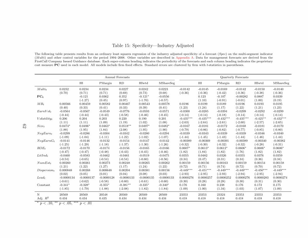
Table 15: Specificity—Industry Adjusted
The following table presents results from an ordinary least squares regression of the industry adjusted specificity of a forecast (Spec) on the multi-segment indicator(Multi) and other control variables for the period 1994–2008. Other variables are described in Appendix A. Data for management forecasts are derived from theFirstCall Company Issued Guidance database. Each super-column heading indicates the periodicity of the forecasts and each column heading indicates the proprietarycost measure PC used in each model. All models include firm fixed effects. Standard errors are clustered by firm with t-statistics in parentheses.
Annual Forecasts Quarterly Forecasts
HI PMargin RD HIwtd MShareSeg HI PMargin RD HIwtd MShareSeg
Multit 0.0232 0.0234 0.0234 0.0227 0.0242 0.0223 -0.0142 -0.0145 -0.0169 -0.0142 -0.0150 -0.0140(0.70) (0.71) (0.71) (0.69) (0.73) (0.68) (-0.36) (-0.36) (-0.42) (-0.36) (-0.38) (-0.36)
PCt -0.121 0.0362 0.352 -0.121∗ -0.0556 0.123 -0.107 -0.00282 0.0887 0.0339(-1.27) (0.45) (0.97) (-1.70) (-0.57) (1.10) (-0.91) (-0.01) (1.00) (0.19)
MBt 0.00566 0.00459 0.00582 0.00467 0.00543 0.00578 0.0196 0.0199 0.0189 0.0196 0.0193 0.0195(0.40) (0.33) (0.41) (0.33) (0.39) (0.41) (1.23) (1.24) (1.17) (1.22) (1.21) (1.23)
EarnV olt -0.0564 -0.0567 -0.0549 -0.0776 -0.0593 -0.0571 -0.0300 -0.0285 -0.0394 -0.0299 -0.0292 -0.0299(-0.44) (-0.44) (-0.43) (-0.58) (-0.46) (-0.45) (-0.14) (-0.14) (-0.18) (-0.14) (-0.14) (-0.14)
V olatilityt 0.206 0.204 0.203 0.220 0.190 0.201 -0.435∗∗∗ -0.435∗∗∗ -0.432∗∗∗ -0.435∗∗∗ -0.425∗∗ -0.432∗∗∗
(1.11) (1.11) (1.09) (1.19) (1.02) (1.08) (-2.63) (-2.64) (-2.61) (-2.60) (-2.57) (-2.65)Sizet 0.0474∗ 0.0496∗ 0.0463∗ 0.0518∗∗ 0.0497∗ 0.0482∗ -0.0167 -0.0181 -0.0172 -0.0168 -0.0181 -0.0170
(1.88) (1.95) (1.84) (2.08) (1.95) (1.90) (-0.79) (-0.86) (-0.82) (-0.77) (-0.85) (-0.80)NegEarnt -0.0299 -0.0286 -0.0304 -0.0342 -0.0280 -0.0294 -0.0339 -0.0343 -0.0339 -0.0339 -0.0346 -0.0340
(-1.09) (-1.04) (-1.11) (-1.22) (-1.02) (-1.07) (-1.44) (-1.45) (-1.43) (-1.44) (-1.46) (-1.44)NegEarnGt -0.0141 -0.0146 -0.0132 -0.0154 -0.0147 -0.0142 -0.00389 -0.00369 -0.00391 -0.00389 -0.00340 -0.00382
(-1.25) (-1.29) (-1.18) (-1.37) (-1.30) (-1.26) (-0.32) (-0.30) (-0.32) (-0.32) (-0.28) (-0.31)ROEt -0.0172 -0.0170 -0.0174 -0.0156 -0.0165 -0.0166 0.0607∗ 0.0613∗ 0.0612∗ 0.0606∗ 0.0606∗ 0.0606∗
(-0.47) (-0.47) (-0.48) (-0.43) (-0.45) (-0.46) (1.82) (1.84) (1.82) (1.76) (1.82) (1.82)LitIndt -0.0460 -0.0583 -0.0462 -0.0461 -0.0519 -0.0475 0.0355 0.0482 0.0326 0.0355 0.0376 0.0359
(-0.54) (-0.65) (-0.54) (-0.54) (-0.60) (-0.56) (0.34) (0.47) (0.31) (0.34) (0.36) (0.34)NumEstt 0.00260 0.00261 0.00273 0.00248 0.00265 0.00262 0.00159 0.00156 0.00163 0.00159 0.00154 0.00158
(1.21) (1.22) (1.27) (1.17) (1.24) (1.22) (0.72) (0.71) (0.74) (0.72) (0.70) (0.72)Dispersiont 0.000848 0.00268 0.000648 0.00204 0.00381 0.00156 -0.449∗∗∗ -0.451∗∗∗ -0.449∗∗∗ -0.449∗∗∗ -0.450∗∗∗ -0.449∗∗∗
(0.02) (0.05) (0.01) (0.04) (0.08) (0.03) (-2.93) (-2.95) (-2.93) (-2.94) (-2.95) (-2.94)Leadt -0.0000134 -0.0000137 -0.0000128 -0.0000133 -0.0000135 -0.0000133 0.0000276 0.0000257 0.0000252 0.0000276 0.0000283 0.0000274
(-0.61) (-0.62) (-0.58) (-0.60) (-0.61) (-0.60) (0.30) (0.28) (0.28) (0.30) (0.31) (0.30)Constant -0.341∗ -0.328∗ -0.355∗ -0.381∗∗ -0.335∗ -0.340∗ 0.176 0.160 0.238 0.176 0.172 0.175
(-1.85) (-1.79) (-1.88) (-2.08) (-1.82) (-1.84) (1.09) (1.00) (1.34) (1.03) (1.07) (1.09)
N 20569 20569 20548 20569 20569 20569 23353 23353 23324 23353 23353 23353Adj. R2 0.434 0.434 0.435 0.434 0.434 0.434 0.418 0.418 0.418 0.418 0.418 0.418∗ p < .10, ∗∗ p < .05, ∗∗∗ p < .01
62
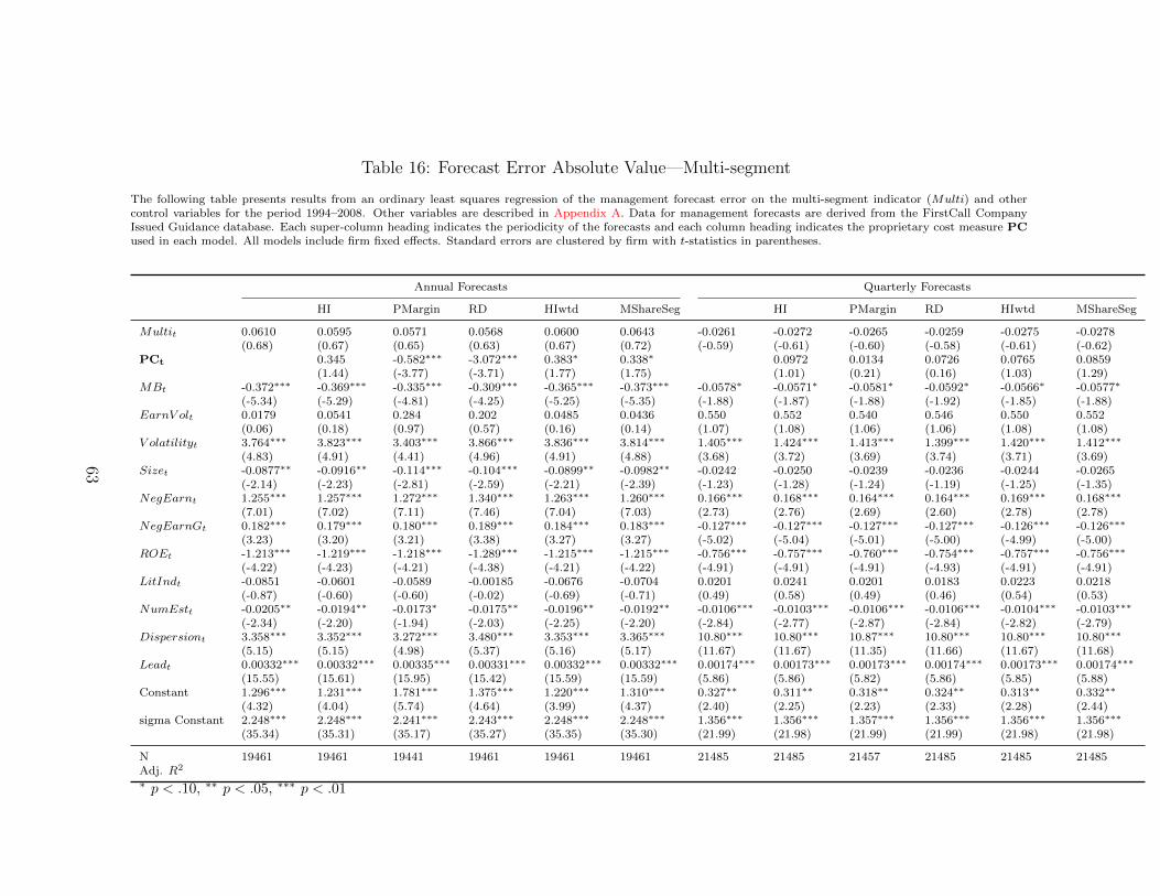
Table 16: Forecast Error Absolute Value—Multi-segment
The following table presents results from an ordinary least squares regression of the management forecast error on the multi-segment indicator (Multi) and othercontrol variables for the period 1994–2008. Other variables are described in Appendix A. Data for management forecasts are derived from the FirstCall CompanyIssued Guidance database. Each super-column heading indicates the periodicity of the forecasts and each column heading indicates the proprietary cost measure PCused in each model. All models include firm fixed effects. Standard errors are clustered by firm with t-statistics in parentheses.
Annual Forecasts Quarterly Forecasts
HI PMargin RD HIwtd MShareSeg HI PMargin RD HIwtd MShareSeg
Multit 0.0610 0.0595 0.0571 0.0568 0.0600 0.0643 -0.0261 -0.0272 -0.0265 -0.0259 -0.0275 -0.0278(0.68) (0.67) (0.65) (0.63) (0.67) (0.72) (-0.59) (-0.61) (-0.60) (-0.58) (-0.61) (-0.62)
PCt 0.345 -0.582∗∗∗ -3.072∗∗∗ 0.383∗ 0.338∗ 0.0972 0.0134 0.0726 0.0765 0.0859(1.44) (-3.77) (-3.71) (1.77) (1.75) (1.01) (0.21) (0.16) (1.03) (1.29)
MBt -0.372∗∗∗ -0.369∗∗∗ -0.335∗∗∗ -0.309∗∗∗ -0.365∗∗∗ -0.373∗∗∗ -0.0578∗ -0.0571∗ -0.0581∗ -0.0592∗ -0.0566∗ -0.0577∗
(-5.34) (-5.29) (-4.81) (-4.25) (-5.25) (-5.35) (-1.88) (-1.87) (-1.88) (-1.92) (-1.85) (-1.88)EarnV olt 0.0179 0.0541 0.284 0.202 0.0485 0.0436 0.550 0.552 0.540 0.546 0.550 0.552
(0.06) (0.18) (0.97) (0.57) (0.16) (0.14) (1.07) (1.08) (1.06) (1.06) (1.08) (1.08)V olatilityt 3.764∗∗∗ 3.823∗∗∗ 3.403∗∗∗ 3.866∗∗∗ 3.836∗∗∗ 3.814∗∗∗ 1.405∗∗∗ 1.424∗∗∗ 1.413∗∗∗ 1.399∗∗∗ 1.420∗∗∗ 1.412∗∗∗
(4.83) (4.91) (4.41) (4.96) (4.91) (4.88) (3.68) (3.72) (3.69) (3.74) (3.71) (3.69)Sizet -0.0877∗∗ -0.0916∗∗ -0.114∗∗∗ -0.104∗∗∗ -0.0899∗∗ -0.0982∗∗ -0.0242 -0.0250 -0.0239 -0.0236 -0.0244 -0.0265
(-2.14) (-2.23) (-2.81) (-2.59) (-2.21) (-2.39) (-1.23) (-1.28) (-1.24) (-1.19) (-1.25) (-1.35)NegEarnt 1.255∗∗∗ 1.257∗∗∗ 1.272∗∗∗ 1.340∗∗∗ 1.263∗∗∗ 1.260∗∗∗ 0.166∗∗∗ 0.168∗∗∗ 0.164∗∗∗ 0.164∗∗∗ 0.169∗∗∗ 0.168∗∗∗
(7.01) (7.02) (7.11) (7.46) (7.04) (7.03) (2.73) (2.76) (2.69) (2.60) (2.78) (2.78)NegEarnGt 0.182∗∗∗ 0.179∗∗∗ 0.180∗∗∗ 0.189∗∗∗ 0.184∗∗∗ 0.183∗∗∗ -0.127∗∗∗ -0.127∗∗∗ -0.127∗∗∗ -0.127∗∗∗ -0.126∗∗∗ -0.126∗∗∗
(3.23) (3.20) (3.21) (3.38) (3.27) (3.27) (-5.02) (-5.04) (-5.01) (-5.00) (-4.99) (-5.00)ROEt -1.213∗∗∗ -1.219∗∗∗ -1.218∗∗∗ -1.289∗∗∗ -1.215∗∗∗ -1.215∗∗∗ -0.756∗∗∗ -0.757∗∗∗ -0.760∗∗∗ -0.754∗∗∗ -0.757∗∗∗ -0.756∗∗∗
(-4.22) (-4.23) (-4.21) (-4.38) (-4.21) (-4.22) (-4.91) (-4.91) (-4.91) (-4.93) (-4.91) (-4.91)LitIndt -0.0851 -0.0601 -0.0589 -0.00185 -0.0676 -0.0704 0.0201 0.0241 0.0201 0.0183 0.0223 0.0218
(-0.87) (-0.60) (-0.60) (-0.02) (-0.69) (-0.71) (0.49) (0.58) (0.49) (0.46) (0.54) (0.53)NumEstt -0.0205∗∗ -0.0194∗∗ -0.0173∗ -0.0175∗∗ -0.0196∗∗ -0.0192∗∗ -0.0106∗∗∗ -0.0103∗∗∗ -0.0106∗∗∗ -0.0106∗∗∗ -0.0104∗∗∗ -0.0103∗∗∗
(-2.34) (-2.20) (-1.94) (-2.03) (-2.25) (-2.20) (-2.84) (-2.77) (-2.87) (-2.84) (-2.82) (-2.79)Dispersiont 3.358∗∗∗ 3.352∗∗∗ 3.272∗∗∗ 3.480∗∗∗ 3.353∗∗∗ 3.365∗∗∗ 10.80∗∗∗ 10.80∗∗∗ 10.87∗∗∗ 10.80∗∗∗ 10.80∗∗∗ 10.80∗∗∗
(5.15) (5.15) (4.98) (5.37) (5.16) (5.17) (11.67) (11.67) (11.35) (11.66) (11.67) (11.68)Leadt 0.00332∗∗∗ 0.00332∗∗∗ 0.00335∗∗∗ 0.00331∗∗∗ 0.00332∗∗∗ 0.00332∗∗∗ 0.00174∗∗∗ 0.00173∗∗∗ 0.00173∗∗∗ 0.00174∗∗∗ 0.00173∗∗∗ 0.00174∗∗∗
(15.55) (15.61) (15.95) (15.42) (15.59) (15.59) (5.86) (5.86) (5.82) (5.86) (5.85) (5.88)Constant 1.296∗∗∗ 1.231∗∗∗ 1.781∗∗∗ 1.375∗∗∗ 1.220∗∗∗ 1.310∗∗∗ 0.327∗∗ 0.311∗∗ 0.318∗∗ 0.324∗∗ 0.313∗∗ 0.332∗∗
(4.32) (4.04) (5.74) (4.64) (3.99) (4.37) (2.40) (2.25) (2.23) (2.33) (2.28) (2.44)sigma Constant 2.248∗∗∗ 2.248∗∗∗ 2.241∗∗∗ 2.243∗∗∗ 2.248∗∗∗ 2.248∗∗∗ 1.356∗∗∗ 1.356∗∗∗ 1.357∗∗∗ 1.356∗∗∗ 1.356∗∗∗ 1.356∗∗∗
(35.34) (35.31) (35.17) (35.27) (35.35) (35.30) (21.99) (21.98) (21.99) (21.99) (21.98) (21.98)
N 19461 19461 19441 19461 19461 19461 21485 21485 21457 21485 21485 21485Adj. R2
∗ p < .10, ∗∗ p < .05, ∗∗∗ p < .01
63
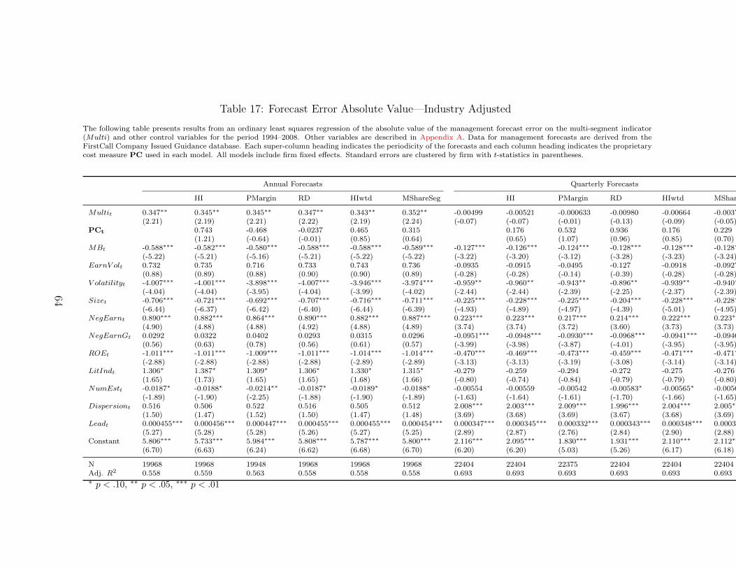
Table 17: Forecast Error Absolute Value—Industry Adjusted
The following table presents results from an ordinary least squares regression of the absolute value of the management forecast error on the multi-segment indicator(Multi) and other control variables for the period 1994–2008. Other variables are described in Appendix A. Data for management forecasts are derived from theFirstCall Company Issued Guidance database. Each super-column heading indicates the periodicity of the forecasts and each column heading indicates the proprietarycost measure PC used in each model. All models include firm fixed effects. Standard errors are clustered by firm with t-statistics in parentheses.
Annual Forecasts Quarterly Forecasts
HI PMargin RD HIwtd MShareSeg HI PMargin RD HIwtd MShareSeg
Multit 0.347∗∗ 0.345∗∗ 0.345∗∗ 0.347∗∗ 0.343∗∗ 0.352∗∗ -0.00499 -0.00521 -0.000633 -0.00980 -0.00664 -0.00374(2.21) (2.19) (2.21) (2.22) (2.19) (2.24) (-0.07) (-0.07) (-0.01) (-0.13) (-0.09) (-0.05)
PCt 0.743 -0.468 -0.0237 0.465 0.315 0.176 0.532 0.936 0.176 0.229(1.21) (-0.64) (-0.01) (0.85) (0.64) (0.65) (1.07) (0.96) (0.85) (0.70)
MBt -0.588∗∗∗ -0.582∗∗∗ -0.580∗∗∗ -0.588∗∗∗ -0.588∗∗∗ -0.589∗∗∗ -0.127∗∗∗ -0.126∗∗∗ -0.124∗∗∗ -0.128∗∗∗ -0.128∗∗∗ -0.128∗∗∗
(-5.22) (-5.21) (-5.16) (-5.21) (-5.22) (-5.22) (-3.22) (-3.20) (-3.12) (-3.28) (-3.23) (-3.24)EarnV olt 0.732 0.735 0.716 0.733 0.743 0.736 -0.0935 -0.0915 -0.0495 -0.127 -0.0918 -0.0927
(0.88) (0.89) (0.88) (0.90) (0.90) (0.89) (-0.28) (-0.28) (-0.14) (-0.39) (-0.28) (-0.28)V olatilityt -4.007∗∗∗ -4.001∗∗∗ -3.898∗∗∗ -4.007∗∗∗ -3.946∗∗∗ -3.974∗∗∗ -0.959∗∗ -0.960∗∗ -0.943∗∗ -0.896∗∗ -0.939∗∗ -0.940∗∗
(-4.04) (-4.04) (-3.95) (-4.04) (-3.99) (-4.02) (-2.44) (-2.44) (-2.39) (-2.25) (-2.37) (-2.39)Sizet -0.706∗∗∗ -0.721∗∗∗ -0.692∗∗∗ -0.707∗∗∗ -0.716∗∗∗ -0.711∗∗∗ -0.225∗∗∗ -0.228∗∗∗ -0.225∗∗∗ -0.204∗∗∗ -0.228∗∗∗ -0.228∗∗∗
(-6.44) (-6.37) (-6.42) (-6.40) (-6.44) (-6.39) (-4.93) (-4.89) (-4.97) (-4.39) (-5.01) (-4.95)NegEarnt 0.890∗∗∗ 0.882∗∗∗ 0.864∗∗∗ 0.890∗∗∗ 0.882∗∗∗ 0.887∗∗∗ 0.223∗∗∗ 0.223∗∗∗ 0.217∗∗∗ 0.214∗∗∗ 0.222∗∗∗ 0.223∗∗∗
(4.90) (4.88) (4.88) (4.92) (4.88) (4.89) (3.74) (3.74) (3.72) (3.60) (3.73) (3.73)NegEarnGt 0.0292 0.0322 0.0402 0.0293 0.0315 0.0296 -0.0951∗∗∗ -0.0948∗∗∗ -0.0930∗∗∗ -0.0968∗∗∗ -0.0941∗∗∗ -0.0946∗∗∗
(0.56) (0.63) (0.78) (0.56) (0.61) (0.57) (-3.99) (-3.98) (-3.87) (-4.01) (-3.95) (-3.95)ROEt -1.011∗∗∗ -1.011∗∗∗ -1.009∗∗∗ -1.011∗∗∗ -1.014∗∗∗ -1.014∗∗∗ -0.470∗∗∗ -0.469∗∗∗ -0.473∗∗∗ -0.459∗∗∗ -0.471∗∗∗ -0.471∗∗∗
(-2.88) (-2.88) (-2.88) (-2.88) (-2.89) (-2.89) (-3.13) (-3.13) (-3.19) (-3.08) (-3.14) (-3.14)LitIndt 1.306∗ 1.387∗ 1.309∗ 1.306∗ 1.330∗ 1.315∗ -0.279 -0.259 -0.294 -0.272 -0.275 -0.276
(1.65) (1.73) (1.65) (1.65) (1.68) (1.66) (-0.80) (-0.74) (-0.84) (-0.79) (-0.79) (-0.80)NumEstt -0.0187∗ -0.0188∗ -0.0214∗∗ -0.0187∗ -0.0189∗ -0.0188∗ -0.00554 -0.00559 -0.00542 -0.00583∗ -0.00565∗ -0.00564∗
(-1.89) (-1.90) (-2.25) (-1.88) (-1.90) (-1.89) (-1.63) (-1.64) (-1.61) (-1.70) (-1.66) (-1.65)Dispersiont 0.516 0.506 0.522 0.516 0.505 0.512 2.008∗∗∗ 2.003∗∗∗ 2.009∗∗∗ 1.996∗∗∗ 2.004∗∗∗ 2.005∗∗∗
(1.50) (1.47) (1.52) (1.50) (1.47) (1.48) (3.69) (3.68) (3.69) (3.67) (3.68) (3.69)Leadt 0.000455∗∗∗ 0.000456∗∗∗ 0.000447∗∗∗ 0.000455∗∗∗ 0.000455∗∗∗ 0.000454∗∗∗ 0.000347∗∗∗ 0.000345∗∗∗ 0.000332∗∗∗ 0.000343∗∗∗ 0.000348∗∗∗ 0.000346∗∗∗
(5.27) (5.28) (5.28) (5.26) (5.27) (5.25) (2.89) (2.87) (2.76) (2.84) (2.90) (2.88)Constant 5.806∗∗∗ 5.733∗∗∗ 5.984∗∗∗ 5.808∗∗∗ 5.787∗∗∗ 5.800∗∗∗ 2.116∗∗∗ 2.095∗∗∗ 1.830∗∗∗ 1.931∗∗∗ 2.110∗∗∗ 2.112∗∗∗
(6.70) (6.63) (6.24) (6.62) (6.68) (6.70) (6.20) (6.20) (5.03) (5.26) (6.17) (6.18)
N 19968 19968 19948 19968 19968 19968 22404 22404 22375 22404 22404 22404Adj. R2 0.558 0.559 0.563 0.558 0.558 0.558 0.693 0.693 0.693 0.693 0.693 0.693∗ p < .10, ∗∗ p < .05, ∗∗∗ p < .01
64

65
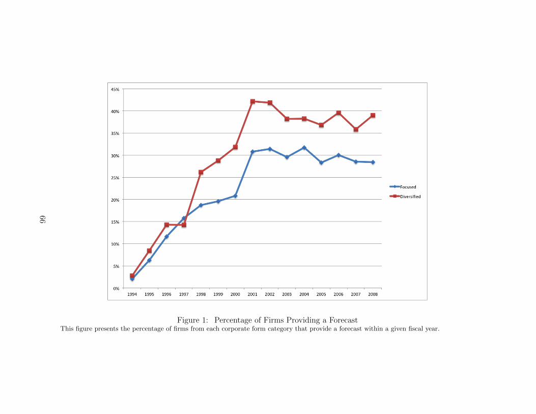
Figure 1: Percentage of Firms Providing a ForecastThis figure presents the percentage of firms from each corporate form category that provide a forecast within a given fiscal year.
66
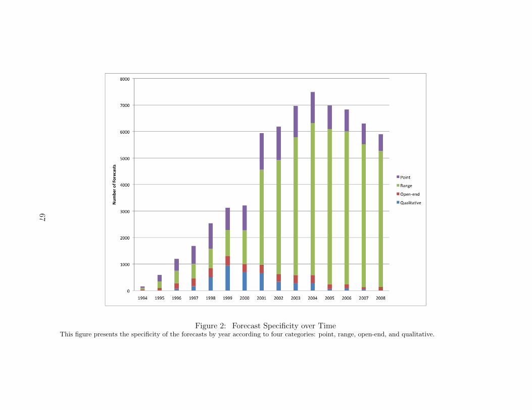
Figure 2: Forecast Specificity over TimeThis figure presents the specificity of the forecasts by year according to four categories: point, range, open-end, and qualitative.
67
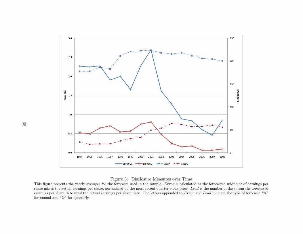
Figure 3: Disclosure Measures over TimeThis figure presents the yearly averages for the forecasts used in the sample. Error is calculated as the forecasted midpoint of earnings pershare minus the actual earnings per share, normalized by the most recent quarter stock price. Lead is the number of days from the forecastedearnings per share date until the actual earnings per share date. The letters appended to Error and Lead indicate the type of forecast: “A”for annual and “Q” for quarterly.
68
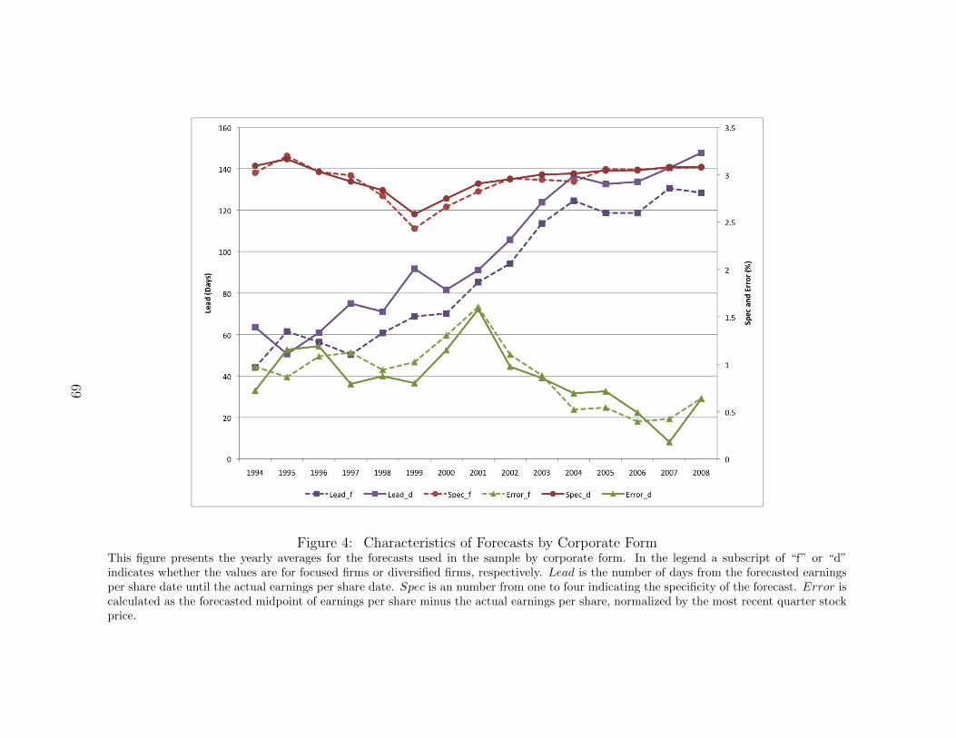
Figure 4: Characteristics of Forecasts by Corporate FormThis figure presents the yearly averages for the forecasts used in the sample by corporate form. In the legend a subscript of “f” or “d”indicates whether the values are for focused firms or diversified firms, respectively. Lead is the number of days from the forecasted earningsper share date until the actual earnings per share date. Spec is an number from one to four indicating the specificity of the forecast. Error iscalculated as the forecasted midpoint of earnings per share minus the actual earnings per share, normalized by the most recent quarter stockprice.
69
Recommended