cosin/mbsMulti-Body Systems & Vehicle Dynamics Simulation
Documentation and User’s Guide
Contents
1 General Remarks 1
1.1 Aims and Scope ofcosin/mbs . . . . . . . . . . . . . . . . . . . . . . . . . . . . . . . . . . . . . 1
1.2 Modeling Approach . . . . . . . . . . . . . . . . . . . . . . . . . . . . . . . . . . . . . . . . . . 1
1.3 Data File Formats and Notation Used in Data Tables Below . . . . . . . . . . . . . . . . . . . . 2
2 Simulation Workbench 3
2.1 Selection of Simulation and Model Data Files . . . . . . . . . . . . . . . . . . . . . . . . . . . . 4
2.2 Simulation Data . . . . . . . . . . . . . . . . . . . . . . . . . . . . . . . . . . . . . . . . . . . . 5
2.2.1 Simulation Data forcosin/mbs . . . . . . . . . . . . . . . . . . . . . . . . . . . . . . . . 5
2.2.2 External Input Signals (Sources) . . . . . . . . . . . . . . . . . . . . . . . . . . . . . . . 10
2.3 Model Data . . . . . . . . . . . . . . . . . . . . . . . . . . . . . . . . . . . . . . . . . . . . . . 11
2.4 Program Execution and Analysis of Results . . . . . . . . . . . . . . . . . . . . . . . . . . . . . 13
3 Modeling and Model Data Files 14
3.1 Model Definition . . . . . . . . . . . . . . . . . . . . . . . . . . . . . . . . . . . . . . . . . . . . 17
3.1.1 Group Definition . . . . . . . . . . . . . . . . . . . . . . . . . . . . . . . . . . . . . . . . 17
3.1.2 Element Definition . . . . . . . . . . . . . . . . . . . . . . . . . . . . . . . . . . . . . . 19
3.2 Element Catalogue . . . . . . . . . . . . . . . . . . . . . . . . . . . . . . . . . . . . . . . . . . 21
4 Interfacing to Models for Road and Wind Velocity 22
4.1 cosin/road . . . . . . . . . . . . . . . . . . . . . . . . . . . . . . . . . . . . . . . . . . . . . . . 22
4.2 cosin/wind . . . . . . . . . . . . . . . . . . . . . . . . . . . . . . . . . . . . . . . . . . . . . . . 22
4.2.1 Typecalm . . . . . . . . . . . . . . . . . . . . . . . . . . . . . . . . . . . . . . . . . . . 22
4.2.2 Typeconstant . . . . . . . . . . . . . . . . . . . . . . . . . . . . . . . . . . . . . . . . 23
4.2.3 Typefile_v_of_t . . . . . . . . . . . . . . . . . . . . . . . . . . . . . . . . . . . . . . 23
4.2.4 Typefile_v_of_x . . . . . . . . . . . . . . . . . . . . . . . . . . . . . . . . . . . . . . 23
4.2.5 Typetable_v_of_t_and_x . . . . . . . . . . . . . . . . . . . . . . . . . . . . . . . . . . 24
4.2.6 Typetable_v_of_x_and_y . . . . . . . . . . . . . . . . . . . . . . . . . . . . . . . . . . 24
4.2.7 Typefunction . . . . . . . . . . . . . . . . . . . . . . . . . . . . . . . . . . . . . . . . 24
Document Revision:2018-2-r17342i
5 ECU Interfacing 24
5.1 Standard ABS . . . . . . . . . . . . . . . . . . . . . . . . . . . . . . . . . . . . . . . . . . . . . 26
5.2 Advanced ABS . . . . . . . . . . . . . . . . . . . . . . . . . . . . . . . . . . . . . . . . . . . . . 27
5.3 ESP (Electronic Stability Program) . . . . . . . . . . . . . . . . . . . . . . . . . . . . . . . . . . 27
5.4 Automatic Four-Wheel Drive Select . . . . . . . . . . . . . . . . . . . . . . . . . . . . . . . . . 28
5.5 ATTS (Automatic Torque Transfer System) . . . . . . . . . . . . . . . . . . . . . . . . . . . . . 29
5.6 LSD (Limited Slip Differential) . . . . . . . . . . . . . . . . . . . . . . . . . . . . . . . . . . . . 30
5.7 Active LSD . . . . . . . . . . . . . . . . . . . . . . . . . . . . . . . . . . . . . . . . . . . . . . . 30
5.8 CLD (Controlled Partially Locking Differentials) . . . . . . . . . . . . . . . . . . . . . . . . . . . 31
5.9 Four-Wheel Steering . . . . . . . . . . . . . . . . . . . . . . . . . . . . . . . . . . . . . . . . . . 31
5.10 EPS (Electronic Power Steering) . . . . . . . . . . . . . . . . . . . . . . . . . . . . . . . . . . . 32
5.11 Advanced EPS . . . . . . . . . . . . . . . . . . . . . . . . . . . . . . . . . . . . . . . . . . . . . 32
5.12 General Force Actuator . . . . . . . . . . . . . . . . . . . . . . . . . . . . . . . . . . . . . . . . 33
6 Interfacing to User-Supplied Driver-Models 33
7 Command Line Invocation 35
8 Coupling to Matlab/Simulink 37
9 Element Catalogue 40
9.1 AC General Actuator with User-Written Control Code . . . . . . . . . . . . . . . . . . . . . . . . 40
9.2 AD Aerodynamic Forces and Moments . . . . . . . . . . . . . . . . . . . . . . . . . . . . . . . . 41
9.3 AS Acceleration Sensor . . . . . . . . . . . . . . . . . . . . . . . . . . . . . . . . . . . . . . . . 44
9.4 BE General Bearing . . . . . . . . . . . . . . . . . . . . . . . . . . . . . . . . . . . . . . . . . . 46
9.5 BJ Ball Joint . . . . . . . . . . . . . . . . . . . . . . . . . . . . . . . . . . . . . . . . . . . . . . 50
9.6 BF Ball Joint Friction Subsystem . . . . . . . . . . . . . . . . . . . . . . . . . . . . . . . . . . . 51
9.6.1 Simple Ball Joint Friction Model . . . . . . . . . . . . . . . . . . . . . . . . . . . . . . . 51
9.6.2 Detailed Ball Joint Friction Model . . . . . . . . . . . . . . . . . . . . . . . . . . . . . . 55
9.6.3 cosin/cb Stand-Alone Simulation Workbench . . . . . . . . . . . . . . . . . . . . . . . . 59
9.7 BO Body . . . . . . . . . . . . . . . . . . . . . . . . . . . . . . . . . . . . . . . . . . . . . . . . 59
9.8 BR Brake System . . . . . . . . . . . . . . . . . . . . . . . . . . . . . . . . . . . . . . . . . . . 59
9.9 CJ Cardan (Hooke) Joint . . . . . . . . . . . . . . . . . . . . . . . . . . . . . . . . . . . . . . . 62
9.10 CS Conceptual Suspension . . . . . . . . . . . . . . . . . . . . . . . . . . . . . . . . . . . . . . . 63
9.11 DI Distance Sensor . . . . . . . . . . . . . . . . . . . . . . . . . . . . . . . . . . . . . . . . . . 67
9.12 DS Damper Strut Assembly . . . . . . . . . . . . . . . . . . . . . . . . . . . . . . . . . . . . . . 68
9.13 DT Drive Torques . . . . . . . . . . . . . . . . . . . . . . . . . . . . . . . . . . . . . . . . . . . 71
9.14 EF External Force . . . . . . . . . . . . . . . . . . . . . . . . . . . . . . . . . . . . . . . . . . . 72
9.15 ET External Torque . . . . . . . . . . . . . . . . . . . . . . . . . . . . . . . . . . . . . . . . . . 73
9.16 FB Flexible Body . . . . . . . . . . . . . . . . . . . . . . . . . . . . . . . . . . . . . . . . . . . . 73
9.17 HM Hydro-Mount Subsystem . . . . . . . . . . . . . . . . . . . . . . . . . . . . . . . . . . . . . 75
9.18 IFInternal Force . . . . . . . . . . . . . . . . . . . . . . . . . . . . . . . . . . . . . . . . . . . . 77
9.19 KC Kinematics&Compliance Output Signals . . . . . . . . . . . . . . . . . . . . . . . . . . . . . 78
9.20 MH Measuring Hub . . . . . . . . . . . . . . . . . . . . . . . . . . . . . . . . . . . . . . . . . . . 82
9.21 PS Propulsion System . . . . . . . . . . . . . . . . . . . . . . . . . . . . . . . . . . . . . . . . . 83
9.22 PT Pushrod-Activated Torsion Bar Springs and Dampers . . . . . . . . . . . . . . . . . . . . . . 90
9.23 RB Rigid Body . . . . . . . . . . . . . . . . . . . . . . . . . . . . . . . . . . . . . . . . . . . . . 94
9.24 RJ Revolute Joint . . . . . . . . . . . . . . . . . . . . . . . . . . . . . . . . . . . . . . . . . . . 101
Document Revision:2018-2-r17342ii

9.25 RO Rod and Straight Pipe . . . . . . . . . . . . . . . . . . . . . . . . . . . . . . . . . . . . . . . 102
9.26 SC Steering Assembly for Conceptual Suspension . . . . . . . . . . . . . . . . . . . . . . . . . . 103
9.27 SD General Spring/Damper . . . . . . . . . . . . . . . . . . . . . . . . . . . . . . . . . . . . . . 105
9.28 SJ Spherical-Spherical Joint . . . . . . . . . . . . . . . . . . . . . . . . . . . . . . . . . . . . . . 109
9.29 SR Steering Assembly, Rack-and-Pinion . . . . . . . . . . . . . . . . . . . . . . . . . . . . . . . 109
9.30 ST Semi-Automatic Transmission . . . . . . . . . . . . . . . . . . . . . . . . . . . . . . . . . . . 115
9.31 TI Tire Model Interface . . . . . . . . . . . . . . . . . . . . . . . . . . . . . . . . . . . . . . . . 117
9.32 TJ Translational Joint . . . . . . . . . . . . . . . . . . . . . . . . . . . . . . . . . . . . . . . . . 122
9.33 TS Torsion-Bar Stabilizer . . . . . . . . . . . . . . . . . . . . . . . . . . . . . . . . . . . . . . . 123
9.34 WL Watt Linkage . . . . . . . . . . . . . . . . . . . . . . . . . . . . . . . . . . . . . . . . . . . . 125
Index 132
Document Revision:2018-2-r17342iii
1 General Remarks
This documentation describes the multi-body and vehicle dynamics simulation packagecosin/mbs. All product or
brand names in mentioned here are trademarks or registered trademarks of their respective holders.
1.1 Aims and Scope ofcosin/mbs
cosin/mbs is designed to be a fast and easy-to-use simulation tool for general multi-body mechanisms, especially
suspensions and vehicle models for both ride comfort and vehicle handling maneuvers. It is equipped with a general
road and tire interface, allowing the combination with several existing tire models likeFTire,FETire,HTire(Magic
Formula in several variants), and others. These tire models can be made available upon request.
By using the comfortable data file formatcosin/io,cosin/mbs is easily parameterized, and combined with other
computation software, like Matlab or Excel, to provide these parameters.
cosin/mbs comes with several sample data files, defining the most important suspension types both for front and
rear axles. If you are licensed to, these will include
• five-link suspensions
• double wishbone suspensions
• several types of McPherson suspensions
• race-car suspensions
• customer-specific axles
• a ‘generic suspension model’ using a general nonlinear force element, situated between wheel and car-body
• the ‘conceptual suspension’ approach, importing files (‘.scf-files’) that describe the full elasto-kinematic
properties of a given suspension, from other vehicle dynamics simulation software.
Likewise,cosin/mbs also enables the user to definecompletely new suspension types in terms of a list ofcos-
in/mbs elements.
cosin/mbs is available for several Linux dialects, as well as for Mac OS X and Windows (XP, Vista, 7, 8; 32 and
64 bit). Even with a detailed rendered 3D on-line animation, it runs considerably faster than real-time.
1.2 Modeling Approach
cosin/mbs is a specializedmulti-body system software, especially focussing on those multi-body elements needed
in vehicle suspension models, including
• flexible bodies
• specialized ‘elasto-kinematic’ elements
• steering assembly models
• drive-train subsystems of different complexity
• brake system element
• aerodynamics
• various road and tire model interfaces.
Document Revision:2018-2-r173421
cosin/mbs uses a tailored implicit integration routine, where only stiff subsystems are integrated implicitly. Even
though implemented in lean and efficient, ‘number-crunching’ ANSI Fortran 90, it consequently observes an
object-oriented approach.
cosin/mbs provides a mechanism to get allpre-load values of all bearings, springs, and so on, in reference position.
To this end,cosin/mbs puts out all pre-load values at the end of a simulation into an output file, and appends the
original input data file. By this, a new, compatible input file is created that carries not only all original vehicle
data, but also all pre-load values to be used in subsequent simulations.
This documentation comprises the following chapters:
• chapter9 introduces and documents the working with thecosin/mbs simulation environment
• chapter3 gives a detailed documentation ofcosin/mbs models and elements
• chapter4 describes the program interfaces to user-provided ECU software
• chapter5 describes the program interfaces to user-provided ECU software
• chapter6 documents the command-line invocation ofcosin/mbs
• chapter7 gives details about usingcosin/mbs within Matlab/Simulink models.
1.3 Data File Formats and Notation Used in Data Tables Below
All data files ofcosin/mbs (apart from imported data files like .csf-files, .tdx-files, and .fem-files) use thecosin/io
syntax that is described in the separate documentationcosin/io User’s Guide. Additional relevant documentation
sheets arecosin/ip User’s Guide (description of several plotting utilities, not yet available),cosin/road User’s Guide
(description of road models), andFTire User’s Guide (documentation of thecosin/mbs compatible tire model
FTire).
In the following chapters, several tables describing input data are included. Most of these tables comprise 4
columns: thedata names, thephysical units, thetypes, and a brief description of theirmeaning. Thereby, the
following data types are distinguished:
Document Revision:2018-2-r173422
i a single integer variablein a vector of integer variables withncomponentsf a single floating point variablefn a vector of floating point variables withn componentssig the name of acosin/ss signal, to be used as input or output signal of an elementst a text string of arbitrary length
Remark: a text string must not contain any blank spaces between the first and the lastnon-blank character
stn a text string of exact lengthnm a marker. Markers either can be defined directly by three numbers (that is, by f3 type data), or
by referring to an entry in the$markers data-block of the .cm-file, specifying the name of therespective marker in this block (cf. chapter4)
sd a spline data-block name. Spline data to be used are to be specified in a spline data- blockwith this name. All splines used incosin/mbs are 2D-splines with natural boundary conditions.That means, they approximate functionsf(x) wheref ′′(x) = 0 for the smallest andlargestx-value that appears in the data table
mo a subsystem or element data-block name. This data type specifies the data-block name of asubsystem or an element of appropriate type
t1 a 1D look-up tablet2 a 2D look-up tablefi a file name, observing the respective operating system’s naming conventionsflag boolean value only, which is true, if the data name appears in the data-block
Table 1: Data types
Mandatory data are marked with (m). If not stated otherwise, all numerical data that are neither mandatory nor
explicitly specified get the default value(s) 0.
2 Simulation Workbench
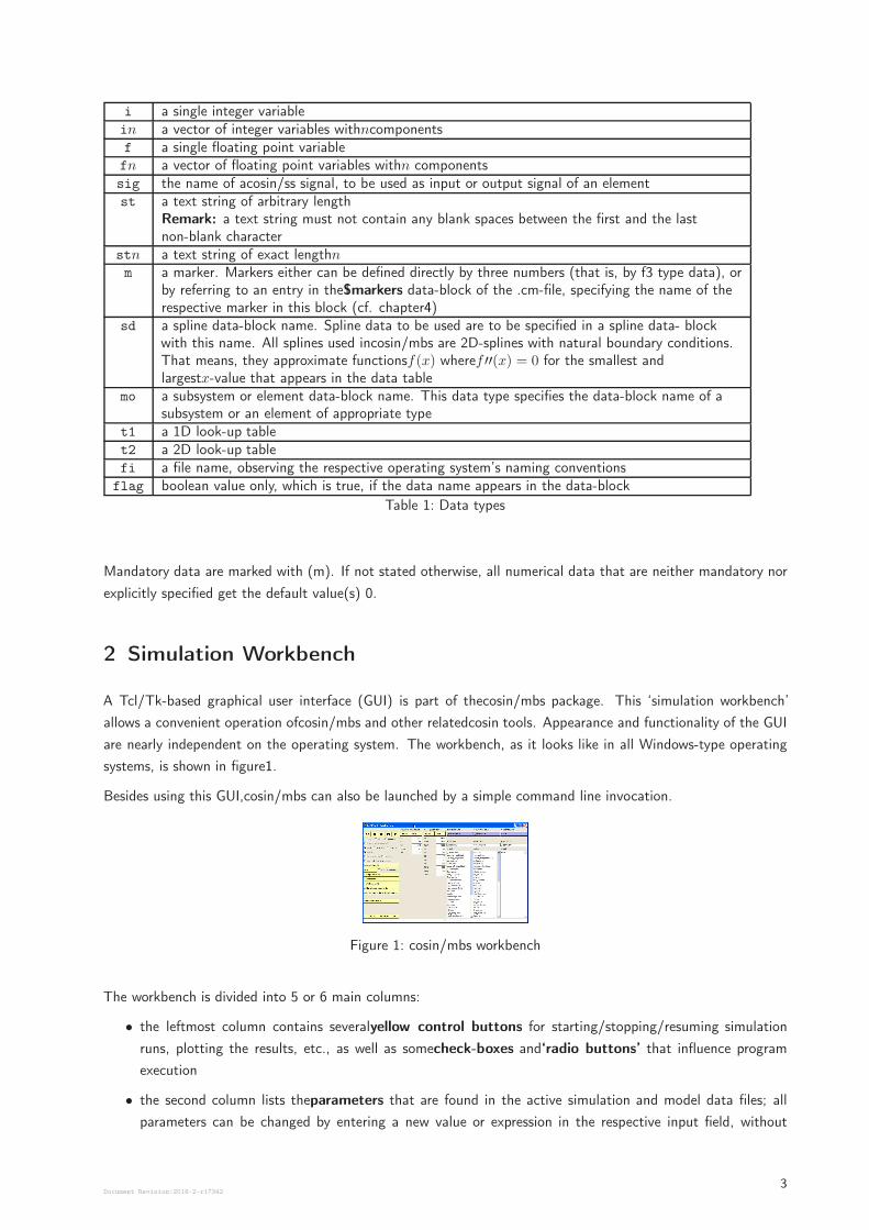
A Tcl/Tk-based graphical user interface (GUI) is part of thecosin/mbs package. This ‘simulation workbench’
allows a convenient operation ofcosin/mbs and other relatedcosin tools. Appearance and functionality of the GUI
are nearly independent on the operating system. The workbench, as it looks like in all Windows-type operating
systems, is shown in figure1.
Besides using this GUI,cosin/mbs can also be launched by a simple command line invocation.
Figure 1: cosin/mbs workbench
The workbench is divided into 5 or 6 main columns:
• the leftmost column contains severalyellow control buttons for starting/stopping/resuming simulation
runs, plotting the results, etc., as well as somecheck-boxes and‘radio buttons’ that influence program
execution
• the second column lists theparameters that are found in the active simulation and model data files; all
parameters can be changed by entering a new value or expression in the respective input field, without
Document Revision:2018-2-r173423
editing the simulation file
• the third and fourth columns show the available simulation and model data files in a respectivefile-box
(simulation and model data files are read by the simulation program after starting the simulation)
• depending on the kind of installation, an optional fifth column shows the available input files for the 3rd-party
modelIPG-Driver, which describes human vehicle control activities
• the file-box of the last column lists output files of actual and previous simulation runs
The upperblue buttons starting with column 3 are calledfunction buttons. Depending on the mouse button
used when clicking, they allow for different ways to process the displayed (‘active’) file. Below, these actions are
described in detail.
A typical simulation run is performed as follows:
• select simulation file and model data file from the respective file-box
• edit and adapt simulation and model data
• click appropriate program execution control buttons
• launch and control program execution, using the GUI’s ‘VCR’ buttons and/or functions provided by an
interactive animation window that appears when simulation starts
• analyze results, for example by using the interactive plot softwarecosin/ip
In the following, these steps are described in more detail.
2.1 Selection of Simulation and Model Data Files
Whencosin/mbs is called for the first time, the file-boxes in columns 3 and 4 of the workbench show several sample
files (cf. figure1). The number and type of these sample files depend on thecosin/mbs options available in your
installation. A specific file isselected by left-clicking the file-name. By doing so, the name of the file will appear
in the blue function button. If required, the file may then beedited by right-clicking the blue function button.
By default, the simulation and model data files are searched for in the directoriessimul andparam, respectively.
These folders themselves are located in the foldercar, a sub-folder of that directory where you installed yourcosin
products. If you keep your data or simulation files in different folders, specify these folders in thepath entry of
column 3 or 4, respectively. You can use every kind of path definition that is valid in the operating system you
are using, for example
• simul\steady_state
• ..\temp\data
• c:\own files\cosin
in Windows-type operating systems, and
• simul/steady_state
• ../temp/data
• $home/own_files/cosin
in Unix-type operating systems.
The sample files shipped withcosin/mbs may serve as a reference while creating new user specified files. In order
to leave the original files unchanged, it is recommended to generate a copy of the reference file first, which covers
Document Revision:2018-2-r173424
the type of maneuver or vehicle needed. For example, to create a vehicle model with a double wishbone front
and rear suspension forcosin/mbs, choose filedw_dw.cm. The procedure tocopy that file is executed in two steps:
first,left-click the file to be copied in the list-box, then hit thespace-bar. Now, a filetest_dw_dw.cm will appear
in the list box. The same procedure holds for creating a user defined simulation file.
Files aredeleted by left-clicking the file name in the list-box, then hitting the‘Del’ key.
2.2 Simulation Data
To adapt the simulation data like simulation time span, number of output steps, kind of on-line animation,
manoeuver to be driven, road profile, etc., to the problem at hand, the corresponding simulation data file (sim-file
for short) is to be edited. Typically, that file consists of the data-blocks
• $simulation
• $sources
• $road_type
Above that, as in allcosin data files, an optional data-block
• $parameters
may be used to parameterize the simulation file, cf.cosin/io documentation. All parameters in this block are
automatically displayed in the second column of the user interface, for convenient access.
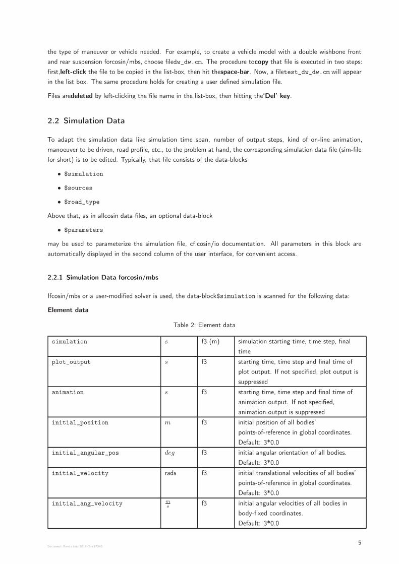
2.2.1 Simulation Data forcosin/mbs
Ifcosin/mbs or a user-modified solver is used, the data-block$simulation is scanned for the following data:
Element data
Table 2: Element data
simulation s f3 (m) simulation starting time, time step, final
time
plot_output s f3 starting time, time step and final time of
plot output. If not specified, plot output is
suppressed
animation s f3 starting time, time step and final time of
animation output. If not specified,
animation output is suppressed
initial_position m f3 initial position of all bodies’
points-of-reference in global coordinates.
Default: 3*0.0
initial_angular_pos deg f3 initial angular orientation of all bodies.
Default: 3*0.0
initial_velocity rads f3 initial translational velocities of all bodies’
points-of-reference in global coordinates.
Default: 3*0.0
initial_ang_velocity ms
f3 initial angular velocities of all bodies in
body-fixed coordinates.
Default: 3*0.0
Document Revision:2018-2-r173425
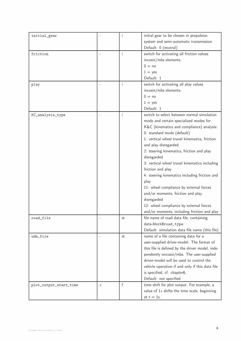
initial_gear - i initial gear to be chosen in propulsion
system and semi-automatic transmission
Default: 0 (neutral)
friction - i switch for activating all friction values
incosin/mbs elements.
0 = no
1 = yes
Default: 1
play - i switch for activating all play values
incosin/mbs elements.
0 = no
1 = yes
Default: 1
KC_analysis_type - i switch to select between normal simulation
mode and certain specialized modes for
K&C (kinematics and compliance) analysis:
0: standard mode (default)
1: vertical wheel travel kinematics, friction
and play disregarded
2: steering kinematics, friction and play
disregarded
3: vertical wheel travel kinematics including
friction and play
4: steering kinematics including friction and
play
11: wheel compliance by external forces
and/or moments, friction and play
disregarded
12: wheel compliance by external forces
and/or moments, including friction and play
road_file - st file name of road data file, containing
data-block$road_type.
Default: simulation data file name (this file)
udm_file - st name of a file containing data for a
user-supplied driver-model. The format of
this file is defined by the driver model, inde-
pendently oncosin/mbs. The user-supplied
driver-model will be used to control the
vehicle operation if and only if this data file
is specified, cf. chapter6.
Default: not specified
plot_output_start_time s f time shift for plot output. For example, a
value of 1s shifts the time scale, beginning
at t = 1s.
Document Revision:2018-2-r173426
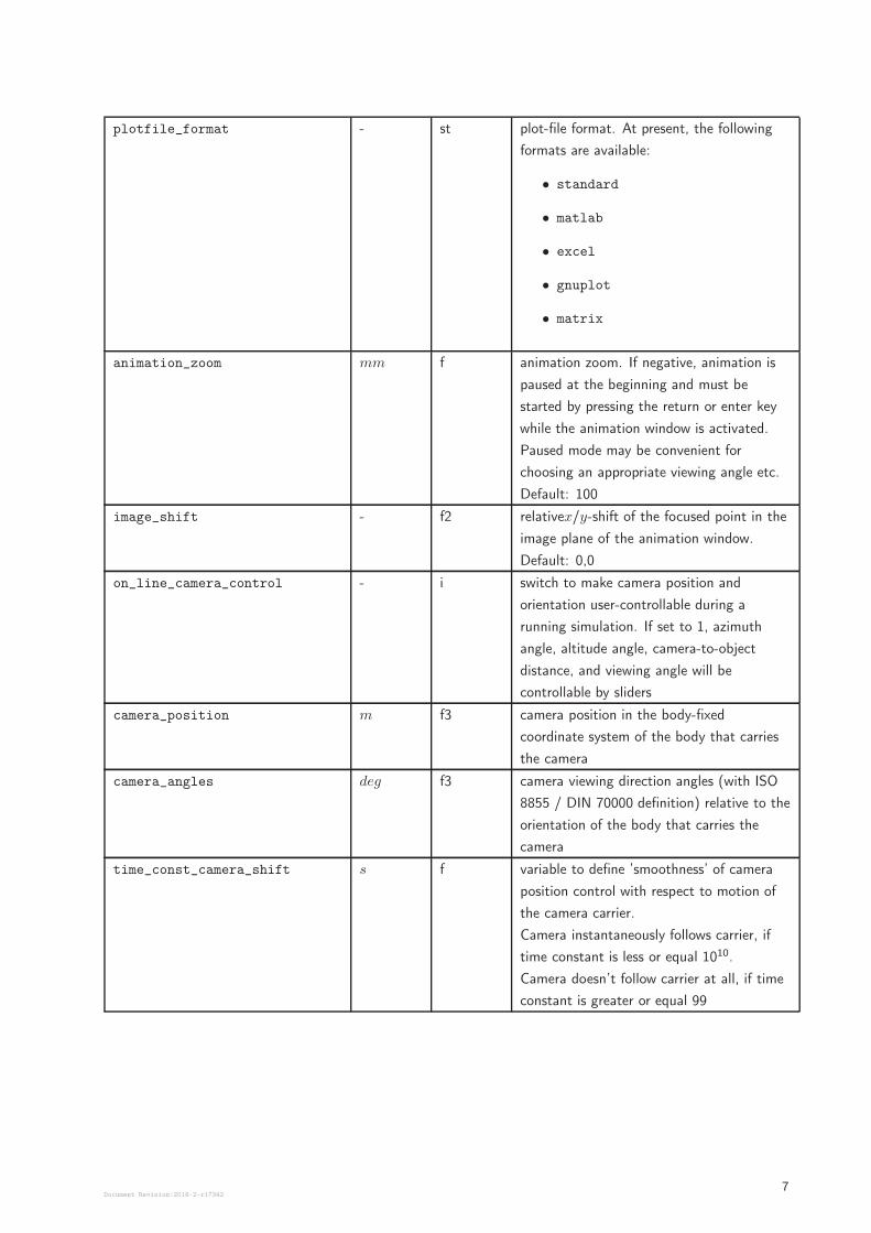
plotfile_format - st plot-file format. At present, the following
formats are available:
• standard
• matlab
• excel
• gnuplot
• matrix
animation_zoom mm f animation zoom. If negative, animation is
paused at the beginning and must be
started by pressing the return or enter key
while the animation window is activated.
Paused mode may be convenient for
choosing an appropriate viewing angle etc.
Default: 100
image_shift - f2 relativex/y-shift of the focused point in the
image plane of the animation window.
Default: 0,0
on_line_camera_control - i switch to make camera position and
orientation user-controllable during a
running simulation. If set to 1, azimuth
angle, altitude angle, camera-to-object
distance, and viewing angle will be
controllable by sliders
camera_position m f3 camera position in the body-fixed
coordinate system of the body that carries
the camera
camera_angles deg f3 camera viewing direction angles (with ISO
8855 / DIN 70000 definition) relative to the
orientation of the body that carries the
camera
time_const_camera_shift s f variable to define ’smoothness’ of camera
position control with respect to motion of
the camera carrier.
Camera instantaneously follows carrier, if
time constant is less or equal 1010.
Camera doesn’t follow carrier at all, if time
constant is greater or equal 99
Document Revision:2018-2-r173427
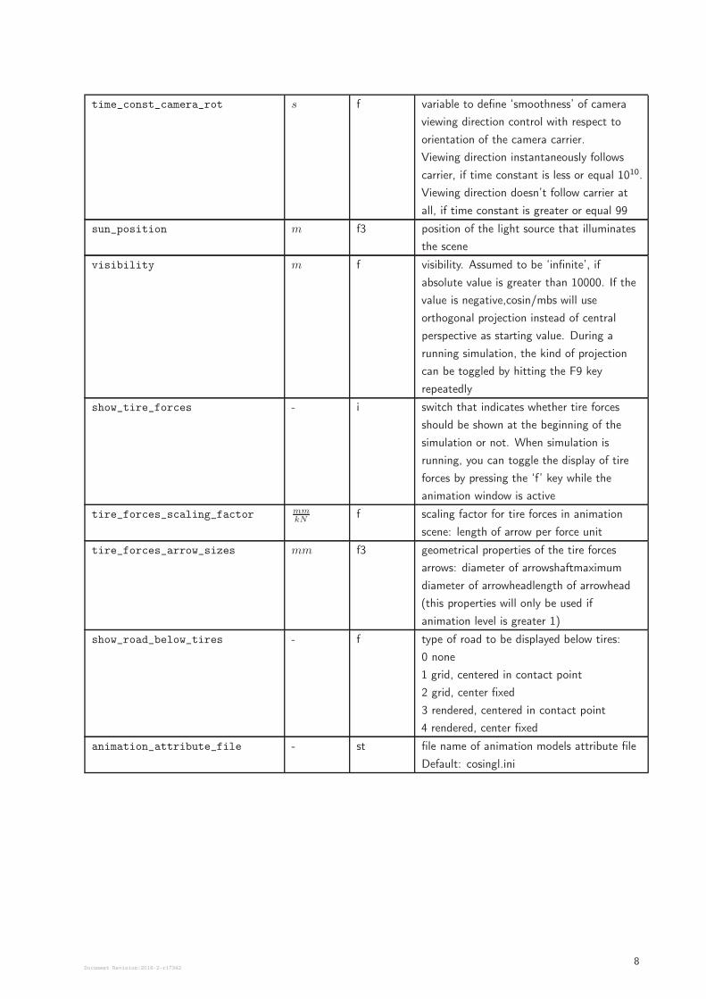
time_const_camera_rot s f variable to define ‘smoothness’ of camera
viewing direction control with respect to
orientation of the camera carrier.
Viewing direction instantaneously follows
carrier, if time constant is less or equal 1010.
Viewing direction doesn’t follow carrier at
all, if time constant is greater or equal 99
sun_position m f3 position of the light source that illuminates
the scene
visibility m f visibility. Assumed to be ‘infinite’, if
absolute value is greater than 10000. If the
value is negative,cosin/mbs will use
orthogonal projection instead of central
perspective as starting value. During a
running simulation, the kind of projection
can be toggled by hitting the F9 key
repeatedly
show_tire_forces - i switch that indicates whether tire forces
should be shown at the beginning of the
simulation or not. When simulation is
running, you can toggle the display of tire
forces by pressing the ‘f’ key while the
animation window is active
tire_forces_scaling_factor mmkN
f scaling factor for tire forces in animation
scene: length of arrow per force unit
tire_forces_arrow_sizes mm f3 geometrical properties of the tire forces
arrows: diameter of arrowshaftmaximum
diameter of arrowheadlength of arrowhead
(this properties will only be used if
animation level is greater 1)
show_road_below_tires - f type of road to be displayed below tires:
0 none
1 grid, centered in contact point
2 grid, center fixed
3 rendered, centered in contact point
4 rendered, center fixed
animation_attribute_file - st file name of animation models attribute file
Default: cosingl.ini
Document Revision:2018-2-r173428
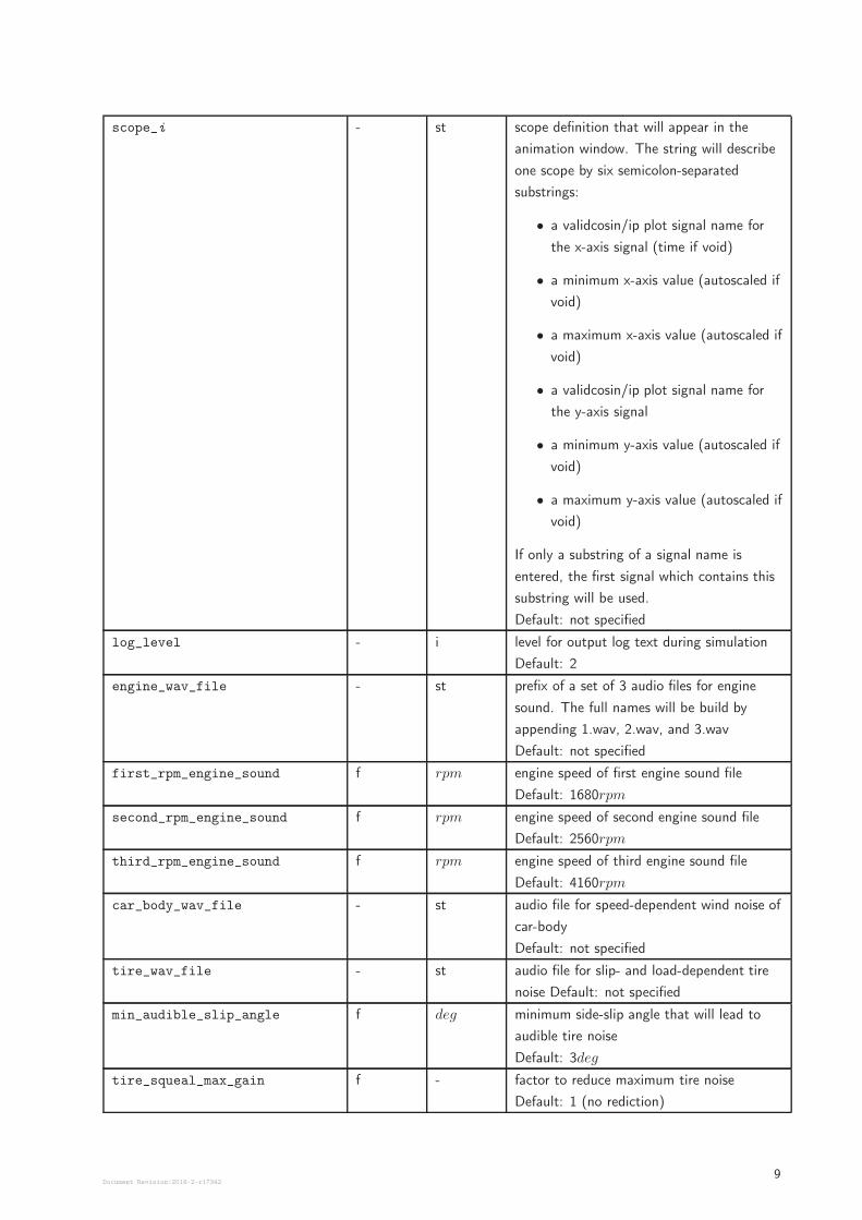
scope_i - st scope definition that will appear in the
animation window. The string will describe
one scope by six semicolon-separated
substrings:
• a validcosin/ip plot signal name for
the x-axis signal (time if void)
• a minimum x-axis value (autoscaled if
void)
• a maximum x-axis value (autoscaled if
void)
• a validcosin/ip plot signal name for
the y-axis signal
• a minimum y-axis value (autoscaled if
void)
• a maximum y-axis value (autoscaled if
void)
If only a substring of a signal name is
entered, the first signal which contains this
substring will be used.
Default: not specified
log_level - i level for output log text during simulation
Default: 2
engine_wav_file - st prefix of a set of 3 audio files for engine
sound. The full names will be build by
appending 1.wav, 2.wav, and 3.wav
Default: not specified
first_rpm_engine_sound f rpm engine speed of first engine sound file
Default: 1680rpm
second_rpm_engine_sound f rpm engine speed of second engine sound file
Default: 2560rpm
third_rpm_engine_sound f rpm engine speed of third engine sound file
Default: 4160rpm
car_body_wav_file - st audio file for speed-dependent wind noise of
car-body
Default: not specified
tire_wav_file - st audio file for slip- and load-dependent tire
noise Default: not specified
min_audible_slip_angle f deg minimum side-slip angle that will lead to
audible tire noise
Default: 3deg
tire_squeal_max_gain f - factor to reduce maximum tire noise
Default: 1 (no rediction)
Document Revision:2018-2-r173429
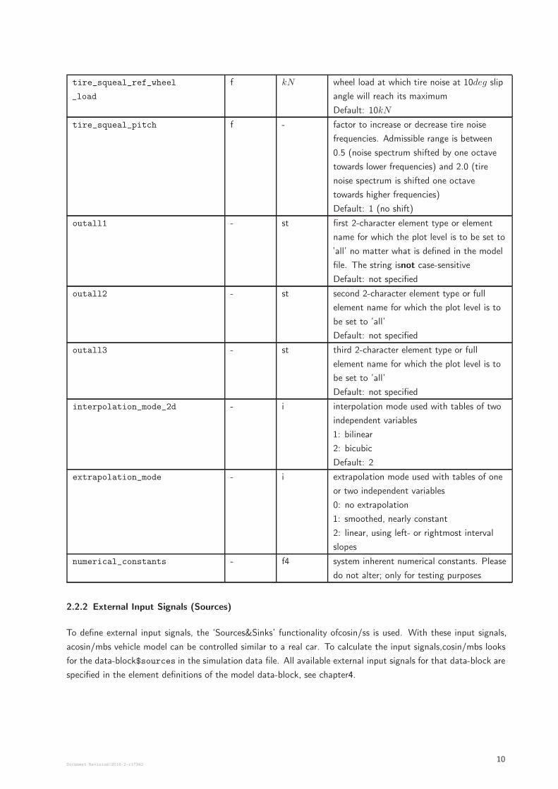
tire_squeal_ref_wheel
_load
f kN wheel load at which tire noise at 10deg slip
angle will reach its maximum
Default: 10kN
tire_squeal_pitch f - factor to increase or decrease tire noise
frequencies. Admissible range is between
0.5 (noise spectrum shifted by one octave
towards lower frequencies) and 2.0 (tire
noise spectrum is shifted one octave
towards higher frequencies)
Default: 1 (no shift)
outall1 - st first 2-character element type or element
name for which the plot level is to be set to
’all’ no matter what is defined in the model
file. The string isnot case-sensitive
Default: not specified
outall2 - st second 2-character element type or full
element name for which the plot level is to
be set to ’all’
Default: not specified
outall3 - st third 2-character element type or full
element name for which the plot level is to
be set to ’all’
Default: not specified
interpolation_mode_2d - i interpolation mode used with tables of two
independent variables
1: bilinear
2: bicubic
Default: 2
extrapolation_mode - i extrapolation mode used with tables of one
or two independent variables
0: no extrapolation
1: smoothed, nearly constant
2: linear, using left- or rightmost interval
slopes
numerical_constants - f4 system inherent numerical constants. Please
do not alter; only for testing purposes
2.2.2 External Input Signals (Sources)
To define external input signals, the ‘Sources&Sinks’ functionality ofcosin/ss is used. With these input signals,
acosin/mbs vehicle model can be controlled similar to a real car. To calculate the input signals,cosin/mbs looks
for the data-block$sources in the simulation data file. All available external input signals for that data-block are
specified in the element definitions of the model data-block, see chapter4.
Document Revision:2018-2-r1734210
2.2.3 Road Profiles, Obstacles, and Wind Velocity
To specify road and wind excitation,cosin/mbs uses the packagescosin/road andcosin/wind. These packages
read the data-blocks$road_type and$wind (either in the simulation data file or, ifroad_file orwind_file,
resp. is assigned a value, in that file). Road profile description with data-block$road_type is described in
the separatecosin/road documentation; whereas wind velocity specification with data-block$wind is presented in
chapter5 below.
2.3 Model Data
To fit the model to the problem at hand, edit the corresponding model data file. The meaning and contents of
model data files are subject of chapter4.
Effects of changes in the geometrical model data can be directly observed and validated by clicking the blue
function button of column 3 with theleft mouse button. Then, the programcosin/show is launched, which
displays the model in design position. Similar to the on-line animation when a simulation is running,cosin/show
can be interactively controlled through zooming in and out, shifting, rotating, and hard-copying. For detailed
information, press theF1-button while the graphics window is active.cosin/show is left by hitting the‘Esc’ key, or
by closing the window.
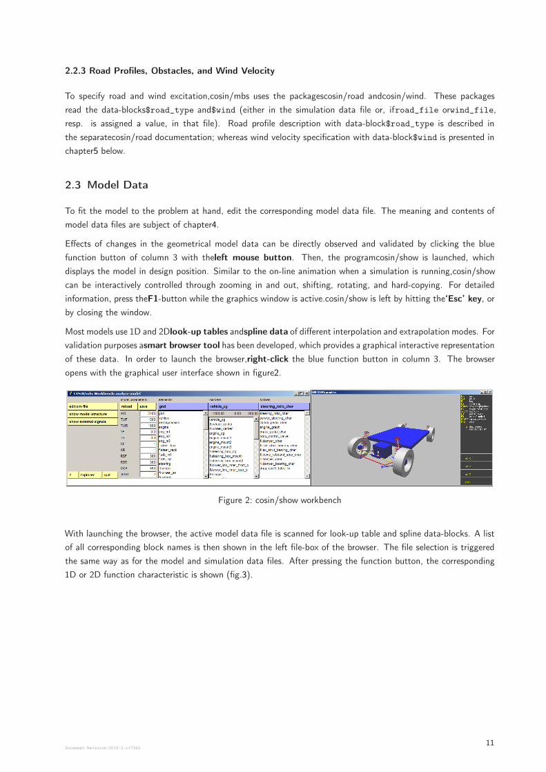
Most models use 1D and 2Dlook-up tables andspline data of different interpolation and extrapolation modes. For
validation purposes asmart browser tool has been developed, which provides a graphical interactive representation
of these data. In order to launch the browser,right-click the blue function button in column 3. The browser
opens with the graphical user interface shown in figure2.
Figure 2: cosin/show workbench
With launching the browser, the active model data file is scanned for look-up table and spline data-blocks. A list
of all corresponding block names is then shown in the left file-box of the browser. The file selection is triggered
the same way as for the model and simulation data files. After pressing the function button, the corresponding
1D or 2D function characteristic is shown (fig.3).
Document Revision:2018-2-r1734211
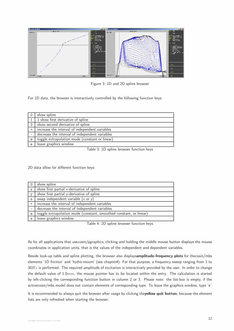
Figure 3: 1D and 2D spline browser
For 1D data, the browser is interactively controlled by the following function keys:
0 show spline1 1 show first derivative of spline2 show second derivative of spline+ increase the interval of independent variables- decrease the interval of independent variablesm toggle extrapolation mode (constant or linear)e leave graphics window
Table 3: 1D spline browser function keys
2D data allow for different function keys:
0 show splinex show first partial x-derivative of spliney show first partial y-derivative of splines swap independent variable (x or y)+ increase the interval of independent variables- decrease the interval of independent variablesm toggle extrapolation mode (constant, smoothed constant, or linear)e leave graphics window
Table 4: 2D spline browser function keys
As for all applications that usecosin/pgraphics, clicking and holding the middle mouse button displays the mouse
coordinates in application units, that is the values of the independent and dependent variables.
Beside look-up table and spline plotting, the browser also displaysamplitude-frequency plots for thecosin/mbs
elements ‘1D friction’ and ‘hydro-mount’ (see chapter4). For that purpose, a frequency sweep ranging from 1 to
30Hz is performed. The required amplitude of excitation is interactively provided by the user. In order to change
the default value of 1.0mm, the mouse pointer has to be located within the entry. The calculation is started
by left-clicking the corresponding function button in column 2 or 3. Please note: the list-box is empty, if the
activecosin/mbs model does not contain elements of corresponding type. To leave the graphics window, type ‘e’.
It is recommended to always quit the browser after usage by clicking theyellow quit button, because the element
lists are only refreshed when starting the browser.
Document Revision:2018-2-r1734212
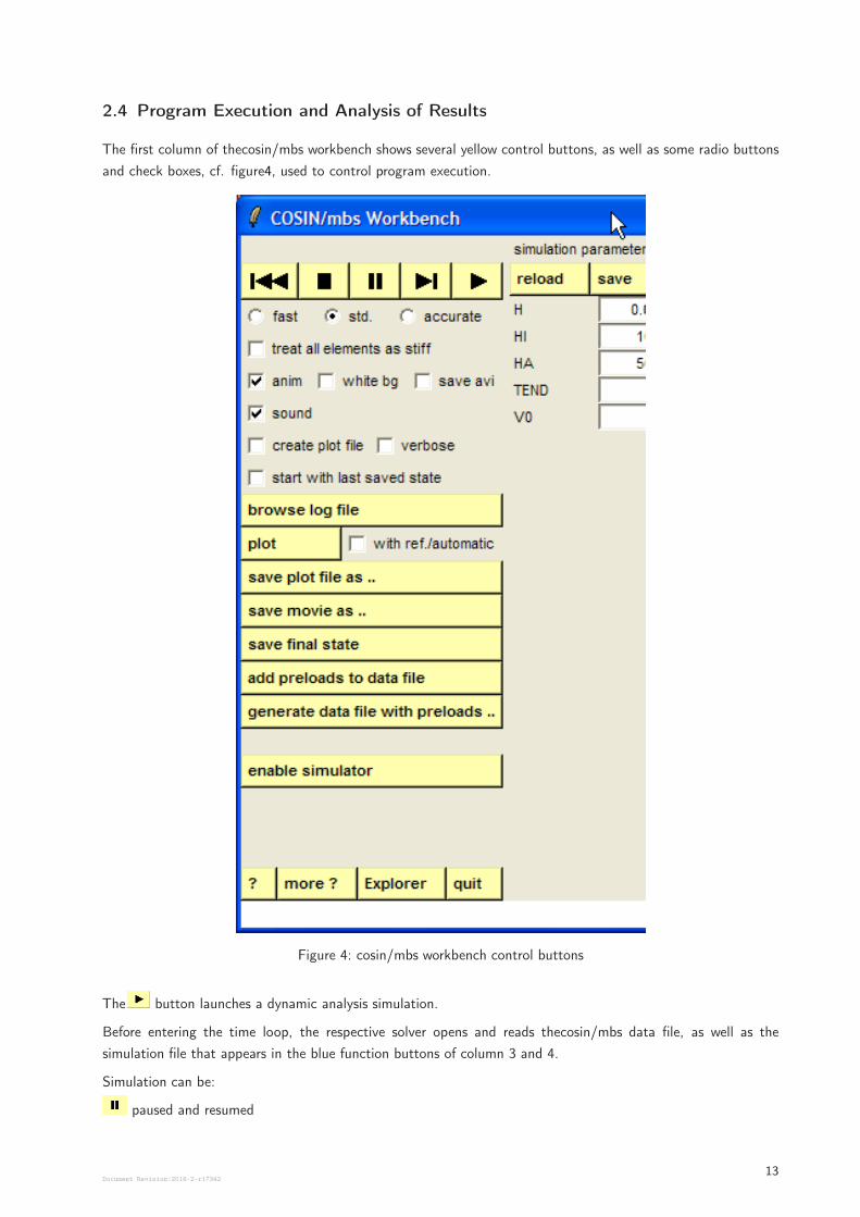
2.4 Program Execution and Analysis of Results
The first column of thecosin/mbs workbench shows several yellow control buttons, as well as some radio buttons
and check boxes, cf. figure4, used to control program execution.
Figure 4: cosin/mbs workbench control buttons
The button launches a dynamic analysis simulation.
Before entering the time loop, the respective solver opens and reads thecosin/mbs data file, as well as the
simulation file that appears in the blue function buttons of column 3 and 4.
Simulation can be:
paused and resumed
Document Revision:2018-2-r1734213
run in single steps
restarted (if not yet finished)
terminated
With the radio buttonsgroup fast,std., andaccurate, the simulation step size defined in data-block$simulation
can be modified:
• fast increases step size by 50%
• std. takes time step exactly as specified in .sim-file
• accurate decreases step size by the same amount
Some further solver parameters can be modified with additional buttons:
• animate toggles interactive on-line animation
• white bg will set background color of animation window to ’white’ instead of gray
• save avi automatically grabs every single frame of the on-line animation and merges them into an .avi-file.
The user will be queried for the name of this file. On-line animation is automatically activated, even if
‘animate’ is not checked
• sound toggles output of engine sound as well as tire and wind noise (provided an OpenAL-compatible sound
card is installed)
• create plot file toggles storage of plot-data. Please note: a plot file must have been created before
clicking the plot-button;
• start with last saved state organizes next simulation to starting with the model in the operating
condition at the time the preceding simulation was terminated. To make this mechanism work properly, the
‘save state’ button has to be clicked after every simulation run, the final states of which are to be taken
as initial conditions for the next run.
For analyzing the results, the plotting toolcosin/ip is provided, which interactively displays the output variables
of the last simulation run. It is launched via the ‘plot’ button. If not only the last output file is to be opened,
but also other ‘reference’ plot-files, check the ‘with reference’ box. In that case, a list will appear before
startingcosin/ip, where additional plot-files can be entered.
The corresponding plot files can be stored by the user, in order to compare different simulation experiments or
model data etc. After left-clicking the button ‘save plot file as..’, a file selection window opens, requesting
the user to specify a file name. Then, the plot file of the preceding simulation is copied to the specified file. The
list box in column 4 shows a list of all previously stored files. In order to opencosin/ip with one of these files
directly, left-click the respective file name first, then left-click the blue function button in column 4.
All available PDF-basedcosin/products documentation chapters can be browsed by left-clicking ’?’, and finally-
cosin/mbs workbench is closed by left-clicking ‘quit’.
3 Modeling and Model Data Files
Acosin/mbs model is described by acosin/mbs model file (‘.cm-file’). Syntactically, a .cm-file is built according
to the syntax rules ofcosin/io (cf. separate documentation). Normally, it consists of
• aparameter definition block
Document Revision:2018-2-r1734214
• amodel definition block, with data sub-blocks that are either
– group definition blocks or
– element definiton blocks
• amarker definition block
• several element data-blocks
Theparameter block is an optional means to parameterize allcosin/io input files, and not a special feature of
only .cm-files. It is described in thecosin/io documentation.
Themodel definition block$modelcontains a list of allcosin/mbs elements to be included to the model, together
with handles of those elements they are linked to. In addition, this data-block carries information specifying where
to find element data, what external input and output signals are provided, and so on. Elements that ‘belong
together’, like all elements that make up a vehicle‘s front suspension, can be grouped together. Having done so,
they can easily be given common properties like plotting or animation model level, coordinate systems, etc. These
groups are also defined in $model.
The optionalmarker definition block$marker contains geometrical data in terms of marker names, together
with their coordinates. These marker names may be used in subsequentcosin/mbs element data-blocks, instead of
numerical values. Marker names may be arbitrarily assigned by the user, to customize acosin/mbs data file. One
advantage of the use of markers is the ability to concentrate the complete geometry information of a mechanical
model in one single data-block.
Element data-blocks contain all data of the elements included in the$model data-block. Normally, to every
such element there belongs at most one element data-block. The contents of these data-blocks are described
below, in the respective element chapters.
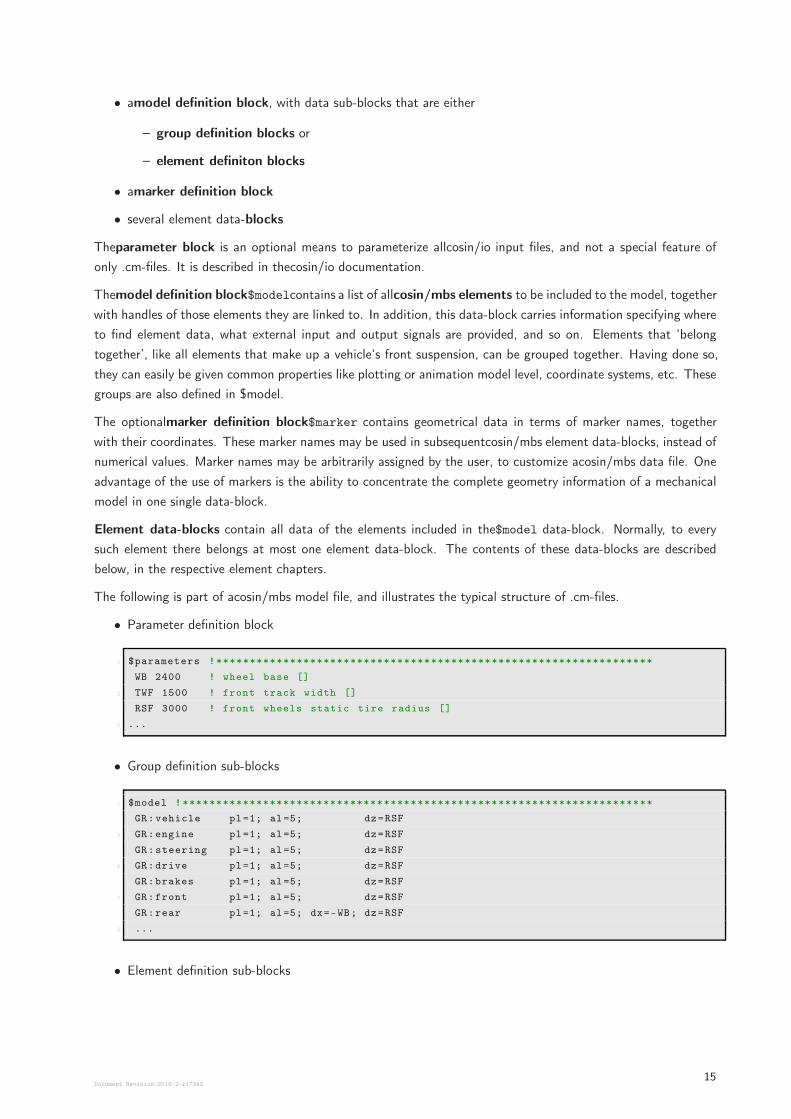
The following is part of acosin/mbs model file, and illustrates the typical structure of .cm-files.
• Parameter definition block
1 $parameters !*****************************************************************
WB 2400 ! wheel base []
3 TWF 1500 ! front track width []
RSF 3000 ! front wheels static tire radius []
5 ...
• Group definition sub-blocks
1 $model ! **********************************************************************
GR:vehicle pl=1; al=5; dz=RSF
3 GR:engine pl=1; al=5; dz=RSF
GR:steering pl=1; al=5; dz=RSF
5 GR:drive pl=1; al=5; dz=RSF
GR:brakes pl=1; al=5; dz=RSF
7 GR:front pl=1; al=5; dz=RSF
GR:rear pl=1; al=5; dx=-WB; dz=RSF
9 ...
• Element definition sub-blocks
Document Revision:2018-2-r1734215
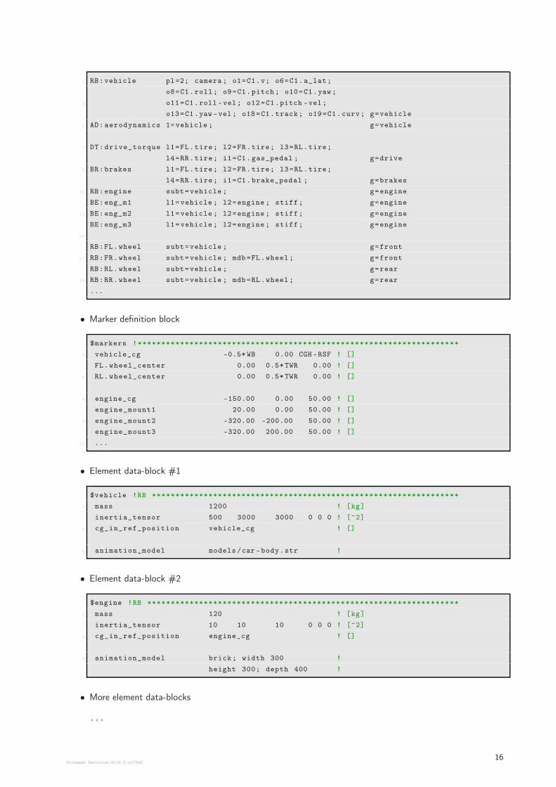
1 RB:vehicle pl=2; camera ; o1=C1.v; o6=C1.a_lat;
o8=C1.roll; o9=C1.pitch ; o10=C1.yaw ;
3 o11=C1.roll -vel; o12 =C1.pitch -vel;
o13=C1.yaw -vel ; o18=C1.track; o19=C1.curv; g=vehicle
5 AD: aerodynamics 1= vehicle ; g=vehicle
7 DT: drive_torque l1=FL.tire; l2=FR.tire; l3=RL.tire;
l4=RR.tire; i1=C1.gas_pedal ; g=drive
9 BR:brakes l1=FL.tire; l2=FR.tire; l3=RL.tire;
l4=RR.tire; i1=C1.brake_pedal ; g=brakes
11 RB:engine subt=vehicle ; g=engine
BE:eng_m1 l1=vehicle ; l2=engine ; stiff; g=engine
13 BE:eng_m2 l1=vehicle ; l2=engine ; stiff; g=engine
BE:eng_m3 l1=vehicle ; l2=engine ; stiff; g=engine
15
RB:FL.wheel subt=vehicle ; g=front
17 RB:FR.wheel subt=vehicle ; mdb =FL.wheel ; g=front
RB:RL.wheel subt=vehicle ; g=rear
19 RB:RR.wheel subt=vehicle ; mdb =RL.wheel ; g=rear
...
• Marker definition block
$markers !********************************************************************
2 vehicle_cg -0.5* WB 0.00 CGH -RSF ! []
FL.wheel_center 0.00 0.5* TWR 0.00 ! []
4 RL.wheel_center 0.00 0.5* TWR 0.00 ! []
6 engine_cg -150.00 0.00 50.00 ! []
engine_mount1 20.00 0.00 50.00 ! []
8 engine_mount2 -320.00 -200.00 50.00 ! []
engine_mount3 -320.00 200.00 50.00 ! []
10 ...
• Element data-block #1
$vehicle !RB *****************************************************************
2 mass 1200 ! [kg]
inertia_tensor 500 3000 3000 0 0 0 ! [^2]
4 cg_in_ref_position vehicle_cg ! []
6 animation_model models /car -body.str !
• Element data-block #2
$engine !RB ******************************************************************
2 mass 120 ! [kg]
inertia_tensor 10 10 10 0 0 0 ! [^2]
4 cg_in_ref_position engine_cg ! []
6 animation_model brick ; width 300 !
height 300; depth 400 !
• More element data-blocks
...
Document Revision:2018-2-r1734216
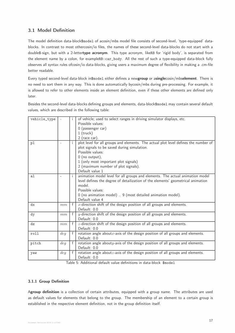
3.1 Model Definition
The model definition data-block$model of acosin/mbs model file consists of second-level, ‘type-equipped’ data-
blocks. In contrast to most othercosin/io files, the names of these second-level data-blocks do not start with a
double$-sign, but with a 2-lettertype acronym. This type acronym, likeRB for ‘rigid body’, is separated from
the element name by a colon, for exampleRB:car_body. All the rest of such a type-equipped data-block fully
observes all syntax rules ofcosin/io data-blocks, giving users a maximum degree of flexibility in making a .cm-file
better readable.
Every typed second-level data-block in$model either defines a newgroup or asinglecosin/mbselement. There is
no need to sort them in any way. This is done automatically bycosin/mbs during pre-processing. For example, it
is allowed to refer to other elements inside an element definition, even if these other elements are defined only
later.
Besides the second-level data-blocks defining groups and elements, data-block$model may contain several default
values, which are described in the following table:
vehicle_type - i of vehicle; used to select ranges in driving simulator displays, etc.Possible values:0 (passenger car)1 (truck)2 (race car).
pl - i plot level for all groups and elements. The actual plot level defines the number ofplot signals to be saved during simulation.Possible values:0 (no output),1 (only most important plot signals)2 (maximum number of plot signals).Default value 1
al - i animation model level for all groups and elements. The actual animation modellevel defines the degree of detailization of the elements’ geometrical animationmodel.Possible values:0 (no animation model) .. 9 (most detailed animation model).Default value 4
dx mm f x-direction shift of the design position of all groups and elements.Default: 0.0
dy mm f y-direction shift of the design position of all groups and elements.Default: 0.0
dz mm f z-direction shift of the design position of all groups and elements.Default: 0.0
roll deg f rotation angle aboutx-axis of the design position of all groups and elements.Default: 0.0
pitch deg f rotation angle abouty-axis of the design position of all groups and elements.Default: 0.0
yaw deg f rotation angle aboutz-axis of the design position of all groups and elements.Default: 0.0
Table 5: Additional default value definitions in data-block $model
3.1.1 Group Definition
Agroup definition is a collection of certain attributes, equipped with a group name. The attributes are used
as default values for elements that belong to the group. The membership of an element to a certain group is
established in the respective element definition, not in the group definition itself.
Document Revision:2018-2-r1734217
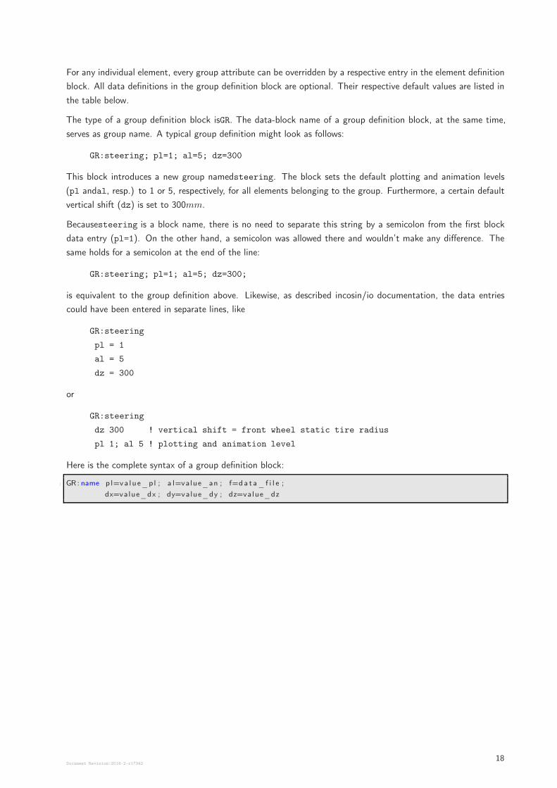
For any individual element, every group attribute can be overridden by a respective entry in the element definition
block. All data definitions in the group definition block are optional. Their respective default values are listed in
the table below.
The type of a group definition block isGR. The data-block name of a group definition block, at the same time,
serves as group name. A typical group definition might look as follows:
GR:steering; pl=1; al=5; dz=300
This block introduces a new group namedsteering. The block sets the default plotting and animation levels
(pl andal, resp.) to 1 or 5, respectively, for all elements belonging to the group. Furthermore, a certain default
vertical shift (dz) is set to 300mm.
Becausesteering is a block name, there is no need to separate this string by a semicolon from the first block
data entry (pl=1). On the other hand, a semicolon was allowed there and wouldn’t make any difference. The
same holds for a semicolon at the end of the line:
GR:steering; pl=1; al=5; dz=300;
is equivalent to the group definition above. Likewise, as described incosin/io documentation, the data entries
could have been entered in separate lines, like
GR:steering
pl = 1
al = 5
dz = 300
or
GR:steering
dz 300 ! vertical shift = front wheel static tire radius
pl 1; al 5 ! plotting and animation level
Here is the complete syntax of a group definition block:
1 GR: name p l=va lue_p l ; a l=value_an ; f=da t a_ f i l e ;
dx=value_dx ; dy=value_dy ; dz=value_dz
Document Revision:2018-2-r1734218
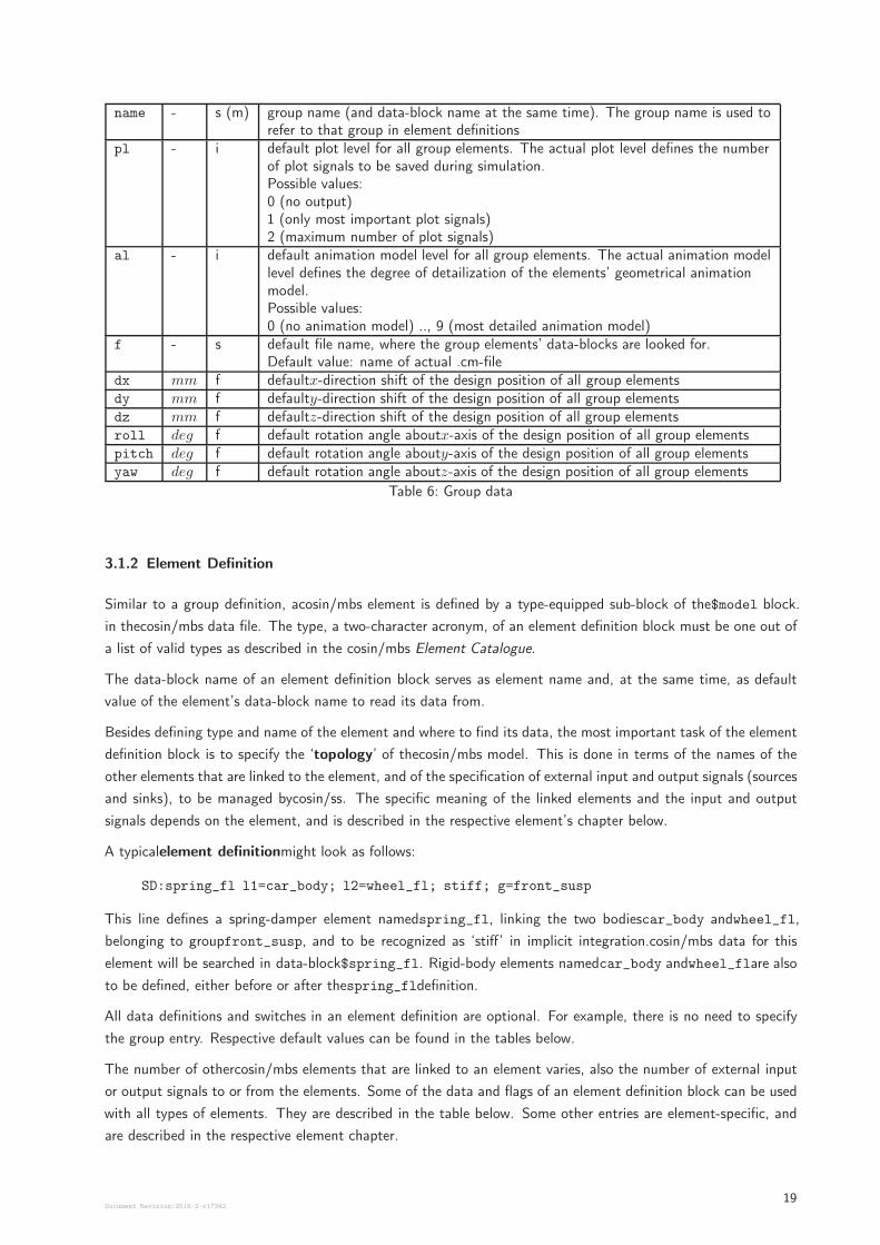
name - s (m) group name (and data-block name at the same time). The group name is used torefer to that group in element definitions
pl - i default plot level for all group elements. The actual plot level defines the numberof plot signals to be saved during simulation.Possible values:0 (no output)1 (only most important plot signals)2 (maximum number of plot signals)
al - i default animation model level for all group elements. The actual animation modellevel defines the degree of detailization of the elements’ geometrical animationmodel.Possible values:0 (no animation model) .., 9 (most detailed animation model)
f - s default file name, where the group elements’ data-blocks are looked for.Default value: name of actual .cm-file
dx mm f defaultx-direction shift of the design position of all group elementsdy mm f defaulty-direction shift of the design position of all group elementsdz mm f defaultz-direction shift of the design position of all group elementsroll deg f default rotation angle aboutx-axis of the design position of all group elementspitch deg f default rotation angle abouty-axis of the design position of all group elementsyaw deg f default rotation angle aboutz-axis of the design position of all group elements
Table 6: Group data
3.1.2 Element Definition
Similar to a group definition, acosin/mbs element is defined by a type-equipped sub-block of the$model block.
in thecosin/mbs data file. The type, a two-character acronym, of an element definition block must be one out of
a list of valid types as described in the cosin/mbs Element Catalogue.
The data-block name of an element definition block serves as element name and, at the same time, as default
value of the element’s data-block name to read its data from.
Besides defining type and name of the element and where to find its data, the most important task of the element
definition block is to specify the ‘topology’ of thecosin/mbs model. This is done in terms of the names of the
other elements that are linked to the element, and of the specification of external input and output signals (sources
and sinks), to be managed bycosin/ss. The specific meaning of the linked elements and the input and output
signals depends on the element, and is described in the respective element’s chapter below.
A typicalelement definitionmight look as follows:
SD:spring_fl l1=car_body; l2=wheel_fl; stiff; g=front_susp
This line defines a spring-damper element namedspring_fl, linking the two bodiescar_body andwheel_fl,
belonging to groupfront_susp, and to be recognized as ‘stiff’ in implicit integration.cosin/mbs data for this
element will be searched in data-block$spring_fl. Rigid-body elements namedcar_body andwheel_flare also
to be defined, either before or after thespring_fldefinition.
All data definitions and switches in an element definition are optional. For example, there is no need to specify
the group entry. Respective default values can be found in the tables below.
The number of othercosin/mbs elements that are linked to an element varies, also the number of external input
or output signals to or from the elements. Some of the data and flags of an element definition block can be used
with all types of elements. They are described in the table below. Some other entries are element-specific, and
are described in the respective element chapter.
Document Revision:2018-2-r1734219
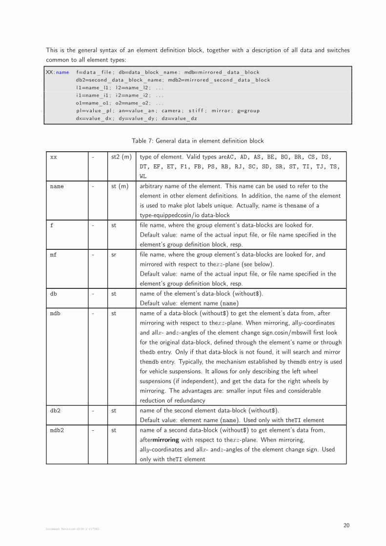
This is the general syntax of an element definition block, together with a description of all data and switches
common to all element types:
XX: name f=da t a_ f i l e ; db=data_block_name : mdb=mirrored_data_block
2 db2=second_data_block_name ; mdb2=mirrored_second_data_block
l 1=name_l1 ; l 2=name_l2 ; . . .
4 i 1=name_i1 ; i 2=name_i2 ; . . .
o1=name_o1 ; o2=name_o2 ; . . .
6 p l=va lue_p l ; an=value_an ; camera ; s t i f f ; m i r r o r ; g=group
dx=value_dx ; dy=value_dy ; dz=value_dz
Table 7: General data in element definition block
xx - st2 (m) type of element. Valid types areAC, AD, AS, BE, BO, BR, CS, DS,
DT, EF, ET, F1, FB, PS, RB, RJ, SC, SD, SR, ST, TI, TJ, TS,
WL
name - st (m) arbitrary name of the element. This name can be used to refer to the
element in other element definitions. In addition, the name of the element
is used to make plot labels unique. Actually, name is thename of a
type-equippedcosin/io data-block
f - st file name, where the group element’s data-blocks are looked for.
Default value: name of the actual input file, or file name specified in the
element’s group definition block, resp.
mf - sr file name, where the group element’s data-blocks are looked for, and
mirrored with respect to thexz-plane (see below).
Default value: name of the actual input file, or file name specified in the
element’s group definition block, resp.
db - st name of the element’s data-block (without$).
Default value: element name (name)
mdb - st name of a data-block (without$) to get the element’s data from, after
mirroring with respect to thexz-plane. When mirroring, ally-coordinates
and allx- andz-angles of the element change sign.cosin/mbswill first look
for the original data-block, defined through the element’s name or through
thedb entry. Only if that data-block is not found, it will search and mirror
themdb entry. Typically, the mechanism established by themdb entry is used
for vehicle suspensions. It allows for only describing the left wheel
suspensions (if independent), and get the data for the right wheels by
mirroring. The advantages are: smaller input files and considerable
reduction of redundancy
db2 - st name of the second element data-block (without$).
Default value: element name (name). Used only with theTI element
mdb2 - st name of a second data-block (without$) to get element’s data from,
aftermirroring with respect to thexz-plane. When mirroring,
ally-coordinates and allx- andz-angles of the element change sign. Used
only with theTI element
Document Revision:2018-2-r1734220
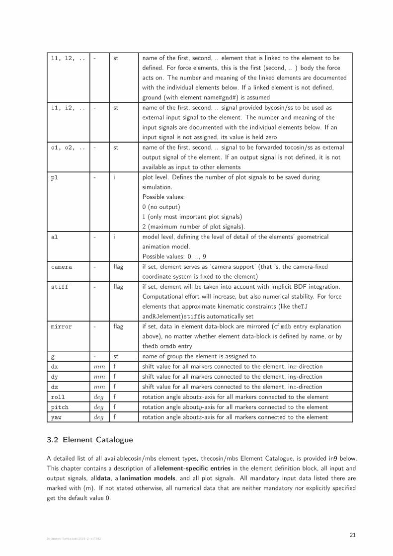
l1, l2, .. - st name of the first, second, .. element that is linked to the element to be
defined. For force elements, this is the first (second, .. ) body the force
acts on. The number and meaning of the linked elements are documented
with the individual elements below. If a linked element is not defined,
ground (with element name#gnd#) is assumed
i1, i2, .. - st name of the first, second, .. signal provided bycosin/ss to be used as
external input signal to the element. The number and meaning of the
input signals are documented with the individual elements below. If an
input signal is not assigned, its value is held zero
o1, o2, .. - st name of the first, second, .. signal to be forwarded tocosin/ss as external
output signal of the element. If an output signal is not defined, it is not
available as input to other elements
pl - i plot level. Defines the number of plot signals to be saved during
simulation.
Possible values:
0 (no output)
1 (only most important plot signals)
2 (maximum number of plot signals).
al - i model level, defining the level of detail of the elements’ geometrical
animation model.
Possible values: 0, .., 9
camera - flag if set, element serves as ‘camera support’ (that is, the camera-fixed
coordinate system is fixed to the element)
stiff - flag if set, element will be taken into account with implicit BDF integration.
Computational effort will increase, but also numerical stability. For force
elements that approximate kinematic constraints (like theTJ
andRJelement)stiffis automatically set
mirror - flag if set, data in element data-block are mirrored (cf.mdb entry explanation
above), no matter whether element data-block is defined by name, or by
thedb ormdb entry
g - st name of group the element is assigned to
dx mm f shift value for all markers connected to the element, inx-direction
dy mm f shift value for all markers connected to the element, iny-direction
dz mm f shift value for all markers connected to the element, inz-direction
roll deg f rotation angle aboutx-axis for all markers connected to the element
pitch deg f rotation angle abouty-axis for all markers connected to the element
yaw deg f rotation angle aboutz-axis for all markers connected to the element
3.2 Element Catalogue
A detailed list of all availablecosin/mbs element types, thecosin/mbs Element Catalogue, is provided in9 below.
This chapter contains a description of allelement-specific entries in the element definition block, all input and
output signals, alldata, allanimation models, and all plot signals. All mandatory input data listed there are
marked with (m). If not stated otherwise, all numerical data that are neither mandatory nor explicitly specified
get the default value 0.
Document Revision:2018-2-r1734221
4 Interfacing to Models for Road and Wind Velocity
cosin/mbs vehicle models can be coupled with models for road surface geometry and other road attributes, as
well as with models for environmental wind velocity.
4.1 cosin/road
The separate packagecosin/road (please refer to respective documentation) provides several models for determin-
istic, stochastic, or measured 2D and 3D road surface geometry and friction attributes. The package includes
models for efficient evaluation of high-resolution measured road surfaces, models for non-rigid surfaces, interfaces
to user-written road models, and more.
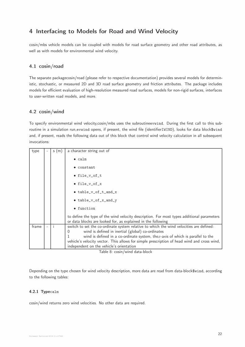
4.2 cosin/wind
To specify environmental wind velocity,cosin/mbs uses the subroutineevwind. During the first call to this sub-
routine in a simulation run,evwind opens, if present, the wind file (identifierIWIND), looks for data block$wind
and, if present, reads the following data out of this block that control wind velocity calculation in all subsequent
invocations:
type - s (m) a character string out of
• calm
• constant
• file_v_of_t
• file_v_of_x
• table_v_of_t_and_x
• table_v_of_x_and_y
• function
to define the type of the wind velocity description. For most types additional parametersor data blocks are looked for, as explained in the following
frame - i switch to set the co-ordinate system relative to which the wind velocities are defined:0 wind is defined in inertial (global) co-ordinates1 wind is defined in a co-ordinate system, thex-axis of which is parallel to thevehicle’s velocity vector. This allows for simple prescription of head wind and cross wind,independent on the vehicle’s orientation
Table 8: cosin/wind data-block
Depending on the type chosen for wind velocity description, more data are read from data-block$wind, according
to the following tables:
4.2.1 Typecalm
cosin/wind returns zero wind velocities. No other data are required.
Document Revision:2018-2-r1734222
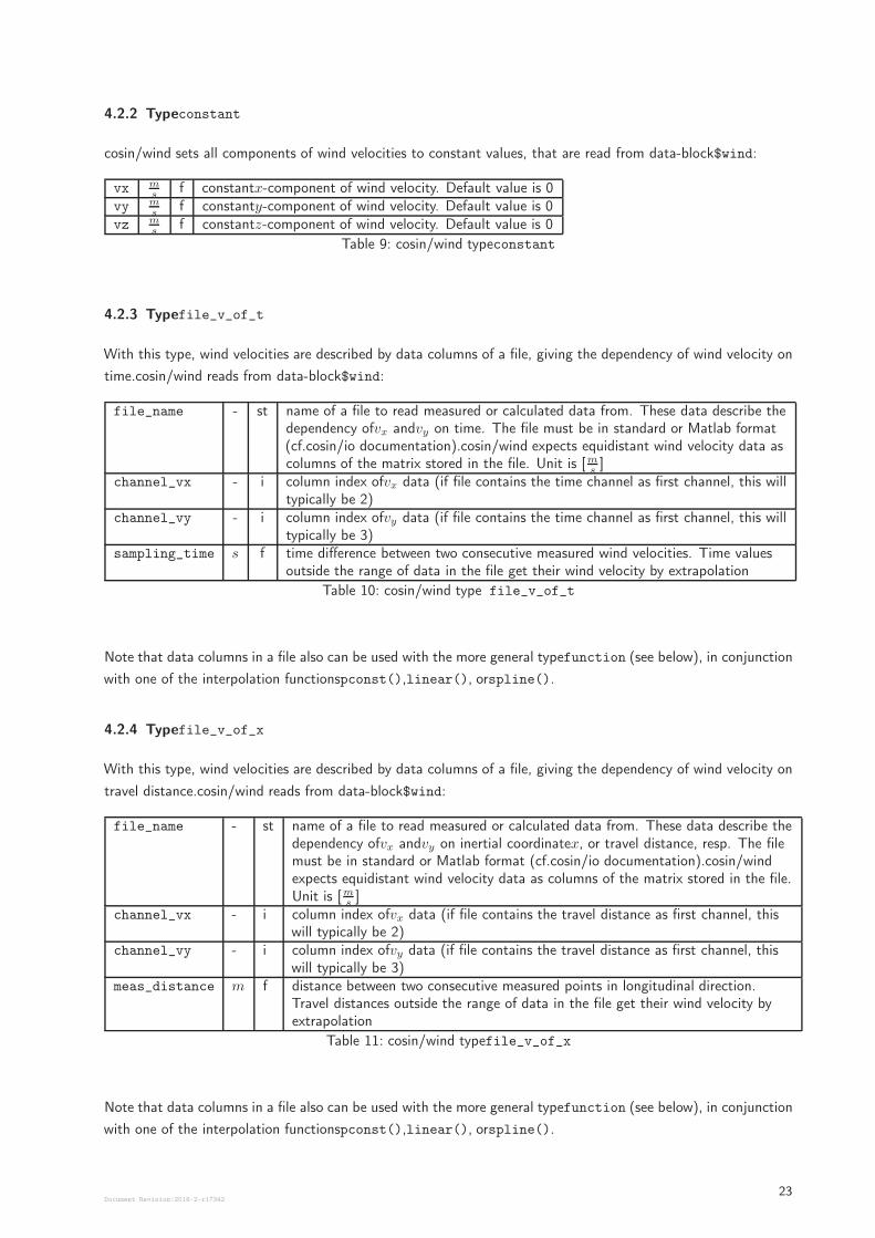
4.2.2 Typeconstant
cosin/wind sets all components of wind velocities to constant values, that are read from data-block$wind:
vx ms
f constantx-component of wind velocity. Default value is 0vy m
sf constanty-component of wind velocity. Default value is 0
vz ms
f constantz-component of wind velocity. Default value is 0
Table 9: cosin/wind typeconstant
4.2.3 Typefile_v_of_t
With this type, wind velocities are described by data columns of a file, giving the dependency of wind velocity on
time.cosin/wind reads from data-block$wind:
file_name - st name of a file to read measured or calculated data from. These data describe thedependency ofvx andvy on time. The file must be in standard or Matlab format(cf.cosin/io documentation).cosin/wind expects equidistant wind velocity data ascolumns of the matrix stored in the file. Unit is [m
s]
channel_vx - i column index ofvx data (if file contains the time channel as first channel, this willtypically be 2)
channel_vy - i column index ofvy data (if file contains the time channel as first channel, this willtypically be 3)
sampling_time s f time difference between two consecutive measured wind velocities. Time valuesoutside the range of data in the file get their wind velocity by extrapolation
Table 10: cosin/wind type file_v_of_t
Note that data columns in a file also can be used with the more general typefunction (see below), in conjunction
with one of the interpolation functionspconst(),linear(), orspline().
4.2.4 Typefile_v_of_x
With this type, wind velocities are described by data columns of a file, giving the dependency of wind velocity on
travel distance.cosin/wind reads from data-block$wind:
file_name - st name of a file to read measured or calculated data from. These data describe thedependency ofvx andvy on inertial coordinatex, or travel distance, resp. The filemust be in standard or Matlab format (cf.cosin/io documentation).cosin/windexpects equidistant wind velocity data as columns of the matrix stored in the file.Unit is [m
s]
channel_vx - i column index ofvx data (if file contains the travel distance as first channel, thiswill typically be 2)
channel_vy - i column index ofvy data (if file contains the travel distance as first channel, thiswill typically be 3)
meas_distance m f distance between two consecutive measured points in longitudinal direction.Travel distances outside the range of data in the file get their wind velocity byextrapolation
Table 11: cosin/wind typefile_v_of_x
Note that data columns in a file also can be used with the more general typefunction (see below), in conjunction
with one of the interpolation functionspconst(),linear(), orspline().
Document Revision:2018-2-r1734223
4.2.5 Typetable_v_of_t_and_x
With this type, wind velocities are described by a 2D look-up table, giving the dependency of wind veloc-
ity on time and on travel distance.cosin/wind looks for the table data in sub-data blocks$vx_of_t_and_x
and$vy_of_t_and_x. For the syntax of spline data definitions, cf.cosin/io documentation.
Note that data columns in a file also can be used with the more general typefunction (see below), in conjunction
with one of the interpolation functionsbilin() orbicub().
4.2.6 Typetable_v_of_x_and_y
With this type, wind velocities are described by a 2D look-up table, giving the dependency of wind velocity on
inertial x/y co-ordinates, or on travel distance and lateral distance to travel path, resp.cosin/wind looks for the
table data in sub-data blocks$vx_of_x_and_y and$vy_of_x_and_y. For the syntax of table data definitions,
cf.cosin/io documentation.
Note that data columns in a file also can be used with the more general typefunction (see below), in conjunction
with one of the interpolation functionsbilin() orbicub().
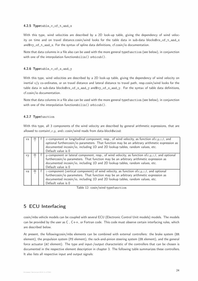
4.2.7 Typefunction
With this type, all 3 components of the wind velocity are described by general arithmetic expressions, that are
allowed to containt,x,y, andz.cosin/wind reads from data-block$wind:
vx ms
f x-component or longitudinal component, resp., of wind velocity, as function ofx,y,z,t, andoptional furthercosin/io parameters. That function may be an arbitrary arithmetic expression asdocumented incosin/io, including 1D and 2D lookup tables, random values, etc.Default value is 0
vy ms
f y-component or lateral component, resp., of wind velocity, as function ofx,y,z,t, and optionalfurthercosin/io parameters. That function may be an arbitrary arithmetic expression asdocumented incosin/io, including 1D and 2D lookup tables, random values, etc.Default value is 0
vz ms
f z-component (vertical component) of wind velocity, as function ofx,y,z,t, and optionalfurthercosin/io parameters. That function may be an arbitrary arithmetic expression asdocumented incosin/io, including 1D and 2D lookup tables, random values, etc.Default value is 0
Table 12: cosin/wind typefunction
5 ECU Interfacing
cosin/mbs vehicle models can be coupled with several ECU (Electronic Control Unit models) models. The models
can be provided by the user as C , C++, or Fortran code. This code must observe certain interfacing rules, which
are described below.
At present, the followingcosin/mbs elements can be combined with external controllers: the brake system (BR
element), the propulsion system (PS element), the rack-and-pinion steering system (SR element), and the general
force actuator (AC element). The type and input-/output characteristic of the controllers that can be chosen is
documented in the respective element description in chapter 3. The following table summarizes these controllers.
It also lists all respective input and output signals:
Document Revision:2018-2-r1734224
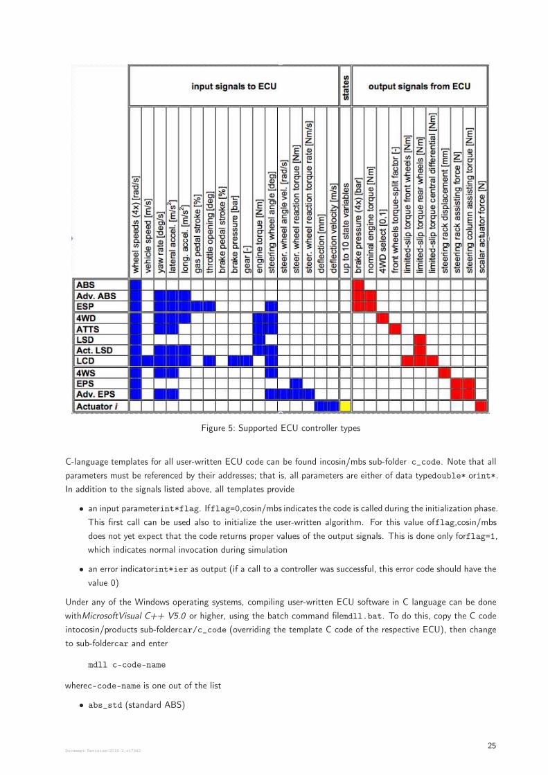
Figure 5: Supported ECU controller types
C-language templates for all user-written ECU code can be found incosin/mbs sub-folder c_code. Note that all
parameters must be referenced by their addresses; that is, all parameters are either of data typedouble* orint*.
In addition to the signals listed above, all templates provide
• an input parameterint*flag. Ifflag=0,cosin/mbs indicates the code is called during the initialization phase.
This first call can be used also to initialize the user-written algorithm. For this value offlag,cosin/mbs
does not yet expect that the code returns proper values of the output signals. This is done only forflag=1,
which indicates normal invocation during simulation
• an error indicatorint*ier as output (if a call to a controller was successful, this error code should have the
value 0)
Under any of the Windows operating systems, compiling user-written ECU software in C language can be done
withMicrosoftVisual C++ V5.0 or higher, using the batch command filemdll.bat. To do this, copy the C code
intocosin/products sub-foldercar/c_code (overriding the template C code of the respective ECU), then change
to sub-foldercar and enter
mdll c-code-name
wherec-code-name is one out of the list
• abs_std (standard ABS)
Document Revision:2018-2-r1734225
• abs_adv (advanced ABS)
• esp (ESP)
• fwd(4WD select)
• atts (front-wheel ATTS)
• lsd_std (conventional LSD)
• lsd_act (active LSD)
• cld(controlled partially locking differentials)
• fws (four-wheel steering 4WS)
• eps_std (simple EPS)
• eps_adv(advanced EPS)
• actuator_i (general force actuator, i =1,..,9)
If compiling and linking was successful, a DLL (Dynamic Link Library) will be generated and copied to thecos-
in/productsbin folder. During a subsequent simulation, if the respective ECU functionality is requested in the
.cm-file, this DLL will be used.
When implementing your code, it is very important to observe the following rule:
If the C-code is called from acosin/mbs element with thestiff property set, then yourcode should not use any
static variables. Such variables can act as ‘hidden’ state variables. Hidden state variables seriously disturb the
implicit integration algorithm, because they make it impossible to properly calculate the Jacobian of the system.
Instead of using static variables, if the callingcosin/mbs element is stiff, your code should ‘remember’ all necessary
values by using thestate array. At present, thestatearray is only available inactuator_i. On demand, all other
ECU interfaces can be extended accordingly.
The following sub-chapters give more details for any of the C-code functions.
5.1 Standard ABS
Prototype
extern void abs_std
(int*flag, double*bp,
double*ws_fl, double*ws_fr, double*ws_rl, double*ws_rr,
double*bp_fl, double*bp_fr, double*bp_rl, double*bp_rr,
int*ier);
Parameter
Document Revision:2018-2-r1734226
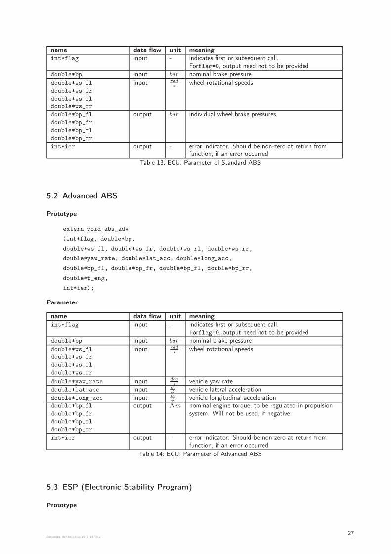
name data flow unit meaningint*flag input - indicates first or subsequent call.
Forflag=0, output need not to be provideddouble*bp input bar nominal brake pressure
double*ws_fl
double*ws_fr
double*ws_rl
double*ws_rr
input rads
wheel rotational speeds
double*bp_fl
double*bp_fr
double*bp_rl
double*bp_rr
output bar individual wheel brake pressures
int*ier output - error indicator. Should be non-zero at return fromfunction, if an error occurred
Table 13: ECU: Parameter of Standard ABS
5.2 Advanced ABS
Prototype
extern void abs_adv
(int*flag, double*bp,
double*ws_fl, double*ws_fr, double*ws_rl, double*ws_rr,
double*yaw_rate, double*lat_acc, double*long_acc,
double*bp_fl, double*bp_fr, double*bp_rl, double*bp_rr,
double*t_eng,
int*ier);
Parameter
name data flow unit meaningint*flag input - indicates first or subsequent call.
Forflag=0, output need not to be provideddouble*bp input bar nominal brake pressure
double*ws_fl
double*ws_fr
double*ws_rl
double*ws_rr
input rads
wheel rotational speeds
double*yaw_rate input degs
vehicle yaw ratedouble*lat_acc input m
s2vehicle lateral acceleration
double*long_acc input ms2
vehicle longitudinal accelerationdouble*bp_fl
double*bp_fr
double*bp_rl
double*bp_rr
output Nm nominal engine torque, to be regulated in propulsionsystem. Will not be used, if negative
int*ier output - error indicator. Should be non-zero at return fromfunction, if an error occurred
Table 14: ECU: Parameter of Advanced ABS
5.3 ESP (Electronic Stability Program)
Prototype
Document Revision:2018-2-r1734227
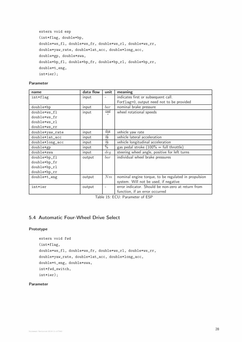
extern void esp
(int*flag, double*bp,
double*ws_fl, double*ws_fr, double*ws_rl, double*ws_rr,
double*yaw_rate, double*lat_acc, double*long_acc,
double*gp, double*swa,
double*bp_fl, double*bp_fr, double*bp_rl, double*bp_rr,
double*t_eng,
int*ier);
Parameter
name data flow unit meaningint*flag input - indicates first or subsequent call.
Forflag=0, output need not to be provideddouble*bp input bar nominal brake pressure
double*ws_fl
double*ws_fr
double*ws_rl
double*ws_rr
input rads
wheel rotational speeds
double*yaw_rate input degs
vehicle yaw ratedouble*lat_acc input m
s2vehicle lateral acceleration
double*long_acc input ms2
vehicle longitudinal accelerationdouble*gp input % gas pedal stroke (100% = full throttle)double*swa input deg steering wheel angle, positive for left turnsdouble*bp_fl
double*bp_fr
double*bp_rl
double*bp_rr
output bar individual wheel brake pressures
double*t_eng output Nm nominal engine torque, to be regulated in propulsionsystem. Will not be used, if negative
int*ier output - error indicator. Should be non-zero at return fromfunction, if an error occurred
Table 15: ECU: Parameter of ESP
5.4 Automatic Four-Wheel Drive Select
Prototype
extern void fwd
(int*flag,
double*ws_fl, double*ws_fr, double*ws_rl, double*ws_rr,
double*yaw_rate, double*lat_acc, double*long_acc,
double*t_eng, double*swa,
int*fwd_switch,
int*ier);
Parameter
Document Revision:2018-2-r1734228
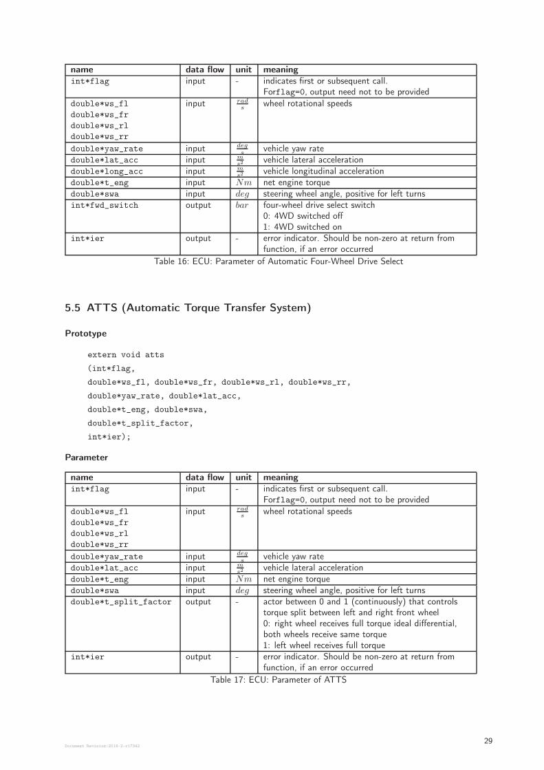
name data flow unit meaningint*flag input - indicates first or subsequent call.
Forflag=0, output need not to be provided
double*ws_fl
double*ws_fr
double*ws_rl
double*ws_rr
input rads
wheel rotational speeds
double*yaw_rate input degs
vehicle yaw ratedouble*lat_acc input m
s2vehicle lateral acceleration
double*long_acc input ms2
vehicle longitudinal accelerationdouble*t_eng input Nm net engine torquedouble*swa input deg steering wheel angle, positive for left turnsint*fwd_switch output bar four-wheel drive select switch
0: 4WD switched off1: 4WD switched on
int*ier output - error indicator. Should be non-zero at return fromfunction, if an error occurred
Table 16: ECU: Parameter of Automatic Four-Wheel Drive Select
5.5 ATTS (Automatic Torque Transfer System)
Prototype
extern void atts
(int*flag,
double*ws_fl, double*ws_fr, double*ws_rl, double*ws_rr,
double*yaw_rate, double*lat_acc,
double*t_eng, double*swa,
double*t_split_factor,
int*ier);
Parameter
name data flow unit meaningint*flag input - indicates first or subsequent call.
Forflag=0, output need not to be provided
double*ws_fl
double*ws_fr
double*ws_rl
double*ws_rr
input rads
wheel rotational speeds
double*yaw_rate input degs
vehicle yaw ratedouble*lat_acc input m
s2vehicle lateral acceleration
double*t_eng input Nm net engine torquedouble*swa input deg steering wheel angle, positive for left turnsdouble*t_split_factor output - actor between 0 and 1 (continuously) that controls
torque split between left and right front wheel0: right wheel receives full torque ideal differential,both wheels receive same torque1: left wheel receives full torque
int*ier output - error indicator. Should be non-zero at return fromfunction, if an error occurred
Table 17: ECU: Parameter of ATTS
Document Revision:2018-2-r1734229
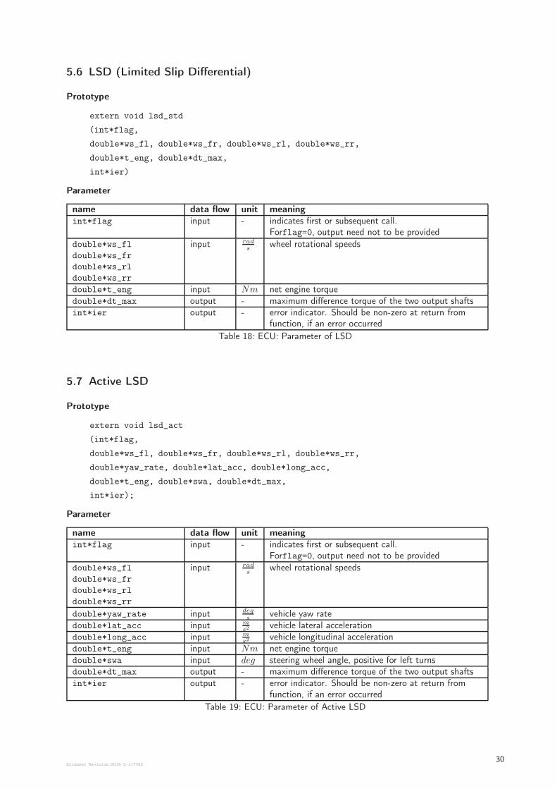
5.6 LSD (Limited Slip Differential)
Prototype
extern void lsd_std
(int*flag,
double*ws_fl, double*ws_fr, double*ws_rl, double*ws_rr,
double*t_eng, double*dt_max,
int*ier)
Parameter
name data flow unit meaningint*flag input - indicates first or subsequent call.
Forflag=0, output need not to be provided
double*ws_fl
double*ws_fr
double*ws_rl
double*ws_rr
input rads
wheel rotational speeds
double*t_eng input Nm net engine torquedouble*dt_max output - maximum difference torque of the two output shaftsint*ier output - error indicator. Should be non-zero at return from
function, if an error occurred
Table 18: ECU: Parameter of LSD
5.7 Active LSD
Prototype
extern void lsd_act
(int*flag,
double*ws_fl, double*ws_fr, double*ws_rl, double*ws_rr,
double*yaw_rate, double*lat_acc, double*long_acc,
double*t_eng, double*swa, double*dt_max,
int*ier);
Parameter
name data flow unit meaningint*flag input - indicates first or subsequent call.
Forflag=0, output need not to be provided
double*ws_fl
double*ws_fr
double*ws_rl
double*ws_rr
input rads
wheel rotational speeds
double*yaw_rate input degs
vehicle yaw ratedouble*lat_acc input m
s2vehicle lateral acceleration
double*long_acc input ms2
vehicle longitudinal accelerationdouble*t_eng input Nm net engine torquedouble*swa input deg steering wheel angle, positive for left turnsdouble*dt_max output - maximum difference torque of the two output shaftsint*ier output - error indicator. Should be non-zero at return from
function, if an error occurred
Table 19: ECU: Parameter of Active LSD
Document Revision:2018-2-r1734230
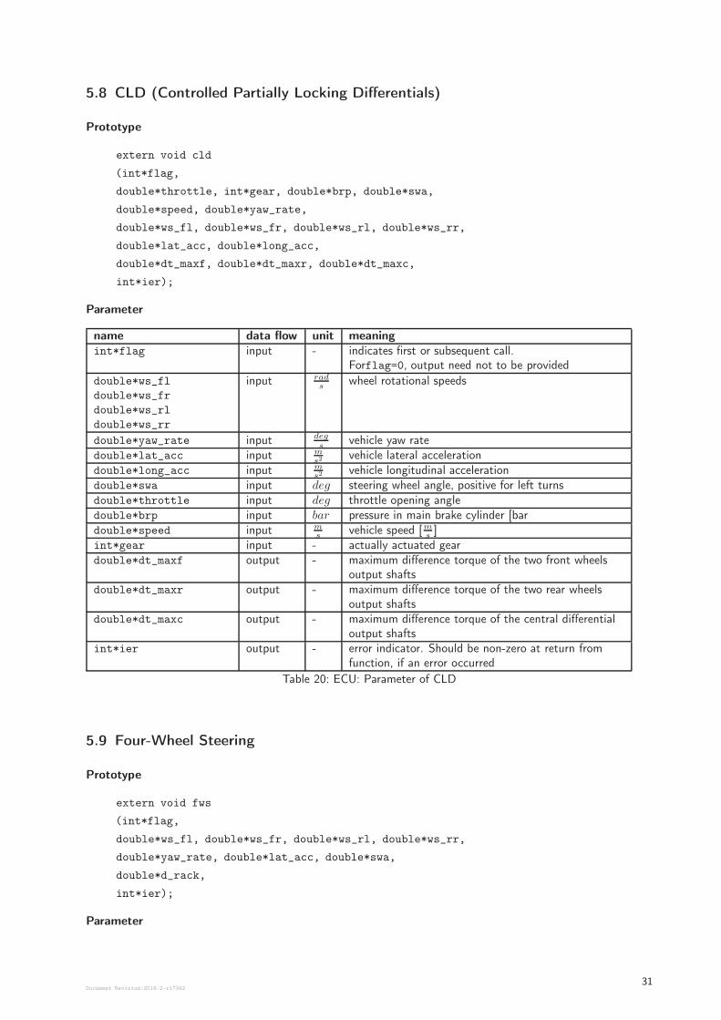
5.8 CLD (Controlled Partially Locking Differentials)
Prototype
extern void cld
(int*flag,
double*throttle, int*gear, double*brp, double*swa,
double*speed, double*yaw_rate,
double*ws_fl, double*ws_fr, double*ws_rl, double*ws_rr,
double*lat_acc, double*long_acc,
double*dt_maxf, double*dt_maxr, double*dt_maxc,
int*ier);
Parameter
name data flow unit meaningint*flag input - indicates first or subsequent call.
Forflag=0, output need not to be provided
double*ws_fl
double*ws_fr
double*ws_rl
double*ws_rr
input rads
wheel rotational speeds
double*yaw_rate input degs
vehicle yaw ratedouble*lat_acc input m
s2vehicle lateral acceleration
double*long_acc input ms2
vehicle longitudinal accelerationdouble*swa input deg steering wheel angle, positive for left turnsdouble*throttle input deg throttle opening angledouble*brp input bar pressure in main brake cylinder [bardouble*speed input m
svehicle speed [m
s]
int*gear input - actually actuated geardouble*dt_maxf output - maximum difference torque of the two front wheels
output shaftsdouble*dt_maxr output - maximum difference torque of the two rear wheels
output shaftsdouble*dt_maxc output - maximum difference torque of the central differential
output shaftsint*ier output - error indicator. Should be non-zero at return from
function, if an error occurred
Table 20: ECU: Parameter of CLD
5.9 Four-Wheel Steering
Prototype
extern void fws
(int*flag,
double*ws_fl, double*ws_fr, double*ws_rl, double*ws_rr,
double*yaw_rate, double*lat_acc, double*swa,
double*d_rack,
int*ier);
Parameter
Document Revision:2018-2-r1734231
name data flow unit meaningint*flag input - indicates first or subsequent call.
Forflag=0, output need not to be provided
double*ws_fl
double*ws_fr
double*ws_rl
double*ws_rr
input rads
wheel rotational speeds
double*yaw_rate input degs
vehicle yaw ratedouble*lat_acc input m
s2vehicle lateral acceleration
double*swa input deg steering wheel angle, positive for left turnsdouble*d_rack output mm rack displacement of rear axle steering assemblyint*ier output - error indicator. Should be non-zero at return from
function, if an error occurred
Table 21: ECU: Parameter of Four-Wheel Steering
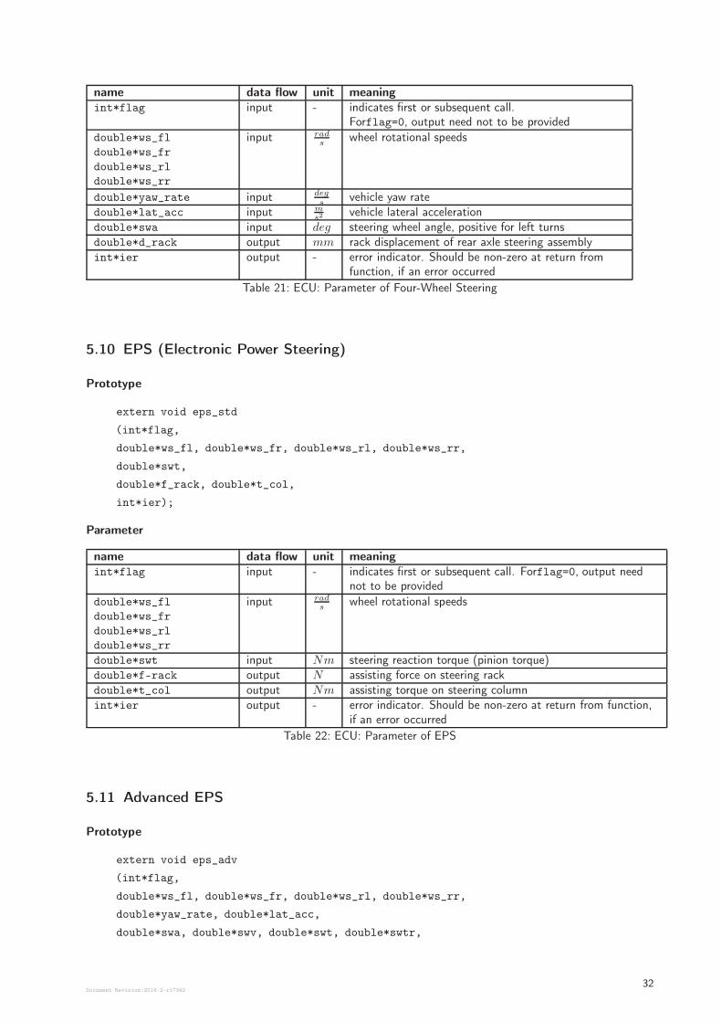
5.10 EPS (Electronic Power Steering)
Prototype
extern void eps_std
(int*flag,
double*ws_fl, double*ws_fr, double*ws_rl, double*ws_rr,
double*swt,
double*f_rack, double*t_col,
int*ier);
Parameter
name data flow unit meaningint*flag input - indicates first or subsequent call. Forflag=0, output need
not to be provided
double*ws_fl
double*ws_fr
double*ws_rl
double*ws_rr
input rads
wheel rotational speeds
double*swt input Nm steering reaction torque (pinion torque)double*f-rack output N assisting force on steering rackdouble*t_col output Nm assisting torque on steering columnint*ier output - error indicator. Should be non-zero at return from function,
if an error occurred
Table 22: ECU: Parameter of EPS
5.11 Advanced EPS
Prototype
extern void eps_adv
(int*flag,
double*ws_fl, double*ws_fr, double*ws_rl, double*ws_rr,
double*yaw_rate, double*lat_acc,
double*swa, double*swv, double*swt, double*swtr,
Document Revision:2018-2-r1734232
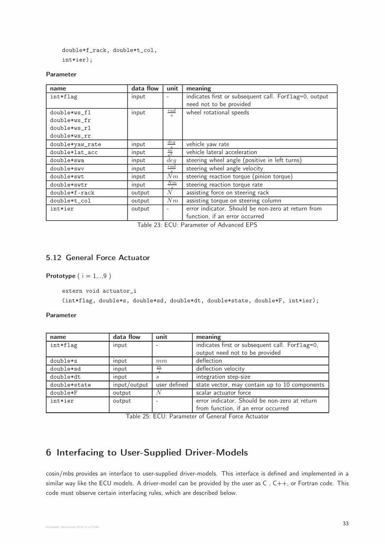
double*f_rack, double*t_col,
int*ier);
Parameter
name data flow unit meaningint*flag input - indicates first or subsequent call. Forflag=0, output
need not to be provided
double*ws_fl
double*ws_fr
double*ws_rl
double*ws_rr
input rads
wheel rotational speeds
double*yaw_rate input degs
vehicle yaw ratedouble*lat_acc input m
s2vehicle lateral acceleration
double*swa input deg steering wheel angle (positive in left turns)
double*swv input rads
steering wheel angle velocitydouble*swt input Nm steering reaction torque (pinion torque)
double*swtr input Nms
steering reaction torque ratedouble*f-rack output N assisting force on steering rackdouble*t_col output Nm assisting torque on steering columnint*ier output - error indicator. Should be non-zero at return from
function, if an error occurred
Table 23: ECU: Parameter of Advanced EPS
5.12 General Force Actuator
Prototype ( i = 1,..,9 )
extern void actuator_i
(int*flag, double*s, double*sd, double*dt, double*state, double*F, int*ier);
Parameter
name data flow unit meaningint*flag input - indicates first or subsequent call. Forflag=0,
output need not to be provideddouble*s input mm deflectiondouble*sd input m
sdeflection velocity
double*dt input s integration step-sizedouble*state input/output user defined state vector, may contain up to 10 componentsdouble*F output N scalar actuator forceint*ier output - error indicator. Should be non-zero at return
from function, if an error occurredTable 25: ECU: Parameter of General Force Actuator
6 Interfacing to User-Supplied Driver-Models
cosin/mbs provides an interface to user-supplied driver-models. This interface is defined and implemented in a
similar way like the ECU models. A driver-model can be provided by the user as C , C++, or Fortran code. This
code must observe certain interfacing rules, which are described below.
Document Revision:2018-2-r1734233
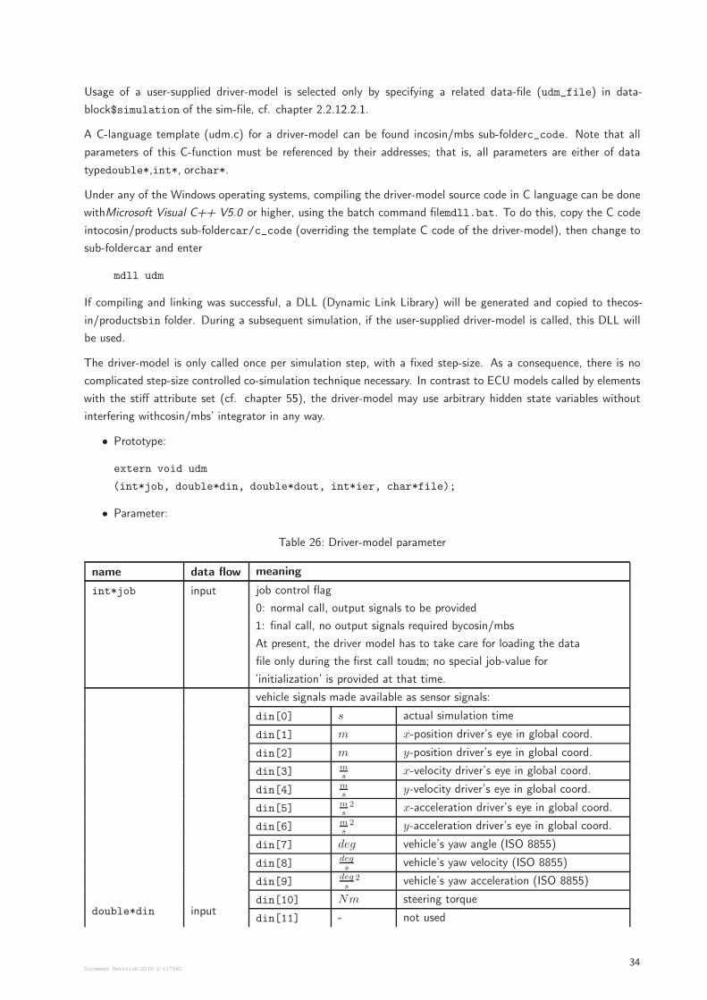
Usage of a user-supplied driver-model is selected only by specifying a related data-file (udm_file) in data-
block$simulation of the sim-file, cf. chapter 2.2.12.2.1.
A C-language template (udm.c) for a driver-model can be found incosin/mbs sub-folderc_code. Note that all
parameters of this C-function must be referenced by their addresses; that is, all parameters are either of data
typedouble*,int*, orchar*.
Under any of the Windows operating systems, compiling the driver-model source code in C language can be done
withMicrosoft Visual C++ V5.0 or higher, using the batch command filemdll.bat. To do this, copy the C code
intocosin/products sub-foldercar/c_code (overriding the template C code of the driver-model), then change to
sub-foldercar and enter
mdll udm
If compiling and linking was successful, a DLL (Dynamic Link Library) will be generated and copied to thecos-
in/productsbin folder. During a subsequent simulation, if the user-supplied driver-model is called, this DLL will
be used.
The driver-model is only called once per simulation step, with a fixed step-size. As a consequence, there is no
complicated step-size controlled co-simulation technique necessary. In contrast to ECU models called by elements
with the stiff attribute set (cf. chapter 55), the driver-model may use arbitrary hidden state variables without
interfering withcosin/mbs’ integrator in any way.
• Prototype:
extern void udm
(int*job, double*din, double*dout, int*ier, char*file);
• Parameter:
Table 26: Driver-model parameter
name data flow meaning
int*job input job control flag
0: normal call, output signals to be provided
1: final call, no output signals required bycosin/mbs
At present, the driver model has to take care for loading the data
file only during the first call toudm; no special job-value for
’initialization’ is provided at that time.
double*din input
vehicle signals made available as sensor signals:
din[0] s actual simulation time
din[1] m x-position driver’s eye in global coord.
din[2] m y-position driver’s eye in global coord.
din[3] ms
x-velocity driver’s eye in global coord.
din[4] ms
y-velocity driver’s eye in global coord.
din[5] ms2 x-acceleration driver’s eye in global coord.
din[6] ms2 y-acceleration driver’s eye in global coord.
din[7] deg vehicle’s yaw angle (ISO 8855)
din[8]degs
vehicle’s yaw velocity (ISO 8855)
din[9]degs
2 vehicle’s yaw acceleration (ISO 8855)
din[10] Nm steering torque
din[11] - not used
Document Revision:2018-2-r1734234
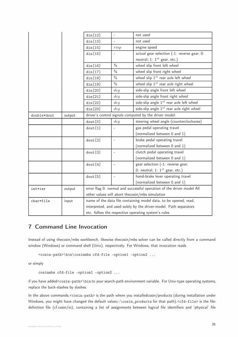
din[12] - not used
din[13] - not used
din[14] rmp engine speed
din[15] - actual gear selection (-1: reverse gear; 0:
neutral; 1: 1st gear, etc.)
din[16] % wheel slip front left wheel
din[17] % wheel slip front right wheel
din[18] % wheel slip 1st rear axle left wheel
din[19] % wheel slip 1st rear axle right wheel
din[20] deg side-slip angle front left wheel
din[21] deg side-slip angle front right wheel
din[22] deg side-slip angle 1st rear axle left wheel
din[23] deg side-slip angle 1st rear axle right wheel
double*dout output driver’s control signals computed by the driver model:
dout[0] deg steering wheel angle (counterclockwise)
dout[1] - gas pedal operating travel
(normalized between 0 and 1)
dout[2] - brake pedal operating travel
(normalized between 0 and 1)
dout[3] - clutch pedal operating travel
(normalized between 0 and 1)
dout[4] - gear selection (-1: reverse gear;
0: neutral; 1: 1st gear, etc.)
dout[5] - hand-brake lever operating travel
(normalized between 0 and 1)
int*ier output error flag 0: normal and successful operation of the driver model All
other values will abort thecosin/mbs simulation
char*file input name of the data file containing model data, to be opened, read,
interpreted, and used solely by the driver-model. Path separators
etc. follow the respective operating system’s rules
7 Command Line Invocation
Instead of using thecosin/mbs workbench, likewise thecosin/mbs solver can be called directly from a command
window (Windows) or command shell (Unix), respectively. For Windows, that invocation reads
<cosin-path>\bin\cosinmbs cfd-file -option1 -option2 ...
or simply
cosinmbs cfd-file -option1 -option2 ...
if you have added<cosin-path>\bin to your search-path environment variable. For Unix-type operating systems,
replace the back-slashes by slashes.
In the above commands,<cosin-path> is the path where you installedcosin/products (during installation under
Windows, you might have changed the default valuec:\cosin_products for that path).<cfd-file> is the file-
definition file (cf.cosin/io), containing a list of assignments between logical file identifiers and ‘physical’ file
Document Revision:2018-2-r1734235
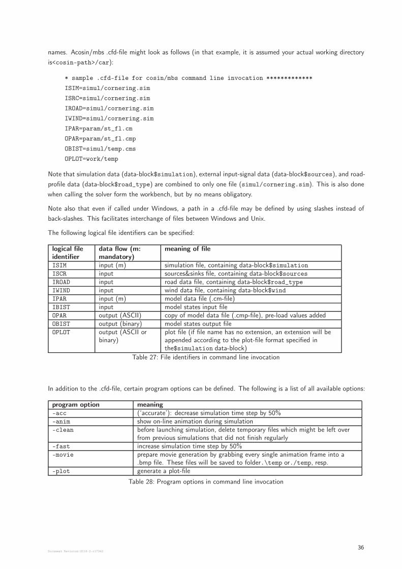
names. Acosin/mbs .cfd-file might look as follows (in that example, it is assumed your actual working directory
is<cosin-path>/car):
* sample .cfd-file for cosin/mbs command line invocation *************
ISIM=simul/cornering.sim
ISRC=simul/cornering.sim
IROAD=simul/cornering.sim
IWIND=simul/cornering.sim
IPAR=param/st_fl.cm
OPAR=param/st_fl.cmp
OBIST=simul/temp.cms
OPLOT=work/temp
Note that simulation data (data-block$simulation), external input-signal data (data-block$sources), and road-
profile data (data-block$road_type) are combined to only one file (simul/cornering.sim). This is also done
when calling the solver form the workbench, but by no means obligatory.
Note also that even if called under Windows, a path in a .cfd-file may be defined by using slashes instead of
back-slashes. This facilitates interchange of files between Windows and Unix.
The following logical file identifiers can be specified:
logical fileidentifier
data flow (m:mandatory)
meaning of file
ISIM input (m) simulation file, containing data-block$simulationISCR input sources&sinks file, containing data-block$sourcesIROAD input road data file, containing data-block$road_typeIWIND input wind data file, containing data-block$windIPAR input (m) model data file (.cm-file)IBIST input model states input fileOPAR output (ASCII) copy of model data file (.cmp-file), pre-load values addedOBIST output (binary) model states output fileOPLOT output (ASCII or
binary)plot file (if file name has no extension, an extension will beappended according to the plot-file format specified inthe$simulation data-block)
Table 27: File identifiers in command line invocation
In addition to the .cfd-file, certain program options can be defined. The following is a list of all available options:
program option meaning-acc (‘accurate’): decrease simulation time step by 50%-anim show on-line animation during simulation-clean before launching simulation, delete temporary files which might be left over
from previous simulations that did not finish regularly-fast increase simulation time step by 50%-movie prepare movie generation by grabbing every single animation frame into a
.bmp file. These files will be saved to folder.\temp or./temp, resp.-plot generate a plot-file
Table 28: Program options in command line invocation
Document Revision:2018-2-r1734236
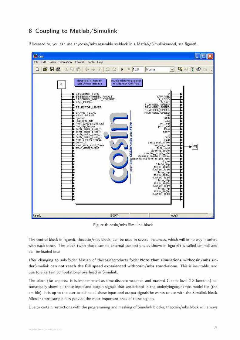
8 Coupling to Matlab/Simulink
If licensed to, you can use anycosin/mbs assembly as block in a Matlab/Simulinkmodel, see figure6.
Figure 6: cosin/mbs Simulink block
The central block in figure6, thecosin/mbs block, can be used in several instances, which will in no way interfere
with each other. The block (with those sample external connections as shown in figure6) is called cm.mdl and
can be loaded into
after changing to sub-folder Matlab of thecosin/products folder.Note that simulations withcosin/mbs un-
derSimulink can not reach the full speed experienced withcosin/mbs stand-alone. This is inevitable, and
due to a certain computational overhead in Simulink.
The block (for experts: it is implemented as time-discrete wrapped and masked C-code level-2 S-function) au-
tomatically shows all those input and output signals that are defined in the underlyingcosin/mbs model file (the
cm-file). It is up to the user to define all those input and output signals he wants to use with the Simulink block.
Allcosin/mbs sample files provide the most important ones of these signals.
Due to certain restrictions with the programming and masking of Simulink blocks, thecosin/mbs block will always
Document Revision:2018-2-r1734237
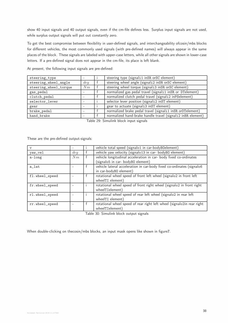
show 40 input signals and 40 output signals, even if the cm-file defines less. Surplus input signals are not used,
while surplus output signals will put out constantly zero.
To get the best compromise between flexibility in user-defined signals, and interchangeability ofcosin/mbs blocks
for different vehicles, the most commonly used signals (with pre-defined names) will always appear in the same
places of the block. These signals are labeled with upper-case letters, while all other signals are shown in lower-case
letters. If a pre-defined signal does not appear in the cm-file, its place is left blank.
At present, the following input signals are pre-defined:
steering_type - i steering type (signali1 inSR orSC element)steering_wheel_angle deg f steering wheel angle (signali2 inSR orSC element)steering_wheel_torque Nm f steering wheel torque (signali3 inSR orSC element)gas_pedal - f normalized gas pedal travel (signali1 inSR or DTelement)clutch_pedal - f normalized clutch pedal travel (signali2 inPSelement)selector_lever - i selector lever position (signali2 inST element)gear - i gear to actuate (signali3 inST element)brake_pedal - f normalized brake pedal travel (signali1 inSR orDTelement)hand_brake - f normalized hand-brake handle travel (signali2 inBR element)
Table 29: Simulink block input signals
These are the pre-defined output-signals:
v - i vehicle total speed (signalo1 in car-bodyBOelement)yaw_vel deg f vehicle yaw velocity (signalo13 in car- bodyBO element)a-long Nm f vehicle longitudinal acceleration in car- body fixed co-ordinates
(signalo5 in car- bodyBO element)a_lat - f vehicle lateral acceleration in car-body fixed co-ordinates (signalo6
in car-bodyBO element)fl.wheel_speed - f rotational wheel speed of front left wheel (signalo2 in front left
wheelTI element)fr.wheel_speed - i rotational wheel speed of front right wheel (signalo2 in front right
wheelTIelement)rl.wheel_speed - i rotational wheel speed of rear left wheel (signalo2 in rear left
wheelTI element)rr.wheel_speed - f rotational wheel speed of rear right left wheel (signalo2in rear right
wheelTIelement)
Table 30: Simulink block output signals
When double-clicking on thecosin/mbs blocks, an input mask opens like shown in figure7.
Document Revision:2018-2-r1734238
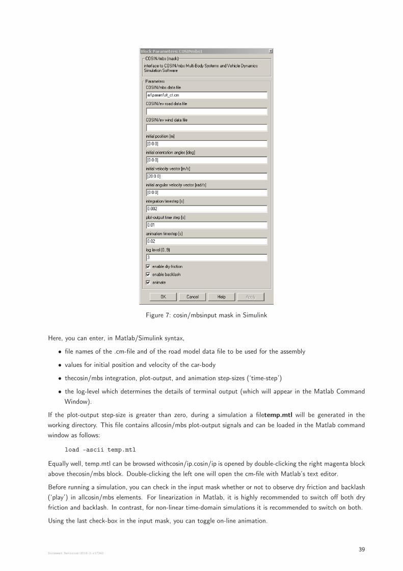
Figure 7: cosin/mbsinput mask in Simulink
Here, you can enter, in Matlab/Simulink syntax,
• file names of the .cm-file and of the road model data file to be used for the assembly
• values for initial position and velocity of the car-body
• thecosin/mbs integration, plot-output, and animation step-sizes (‘time-step’)
• the log-level which determines the details of terminal output (which will appear in the Matlab Command
Window).
If the plot-output step-size is greater than zero, during a simulation a filetemp.mtl will be generated in the
working directory. This file contains allcosin/mbs plot-output signals and can be loaded in the Matlab command
window as follows:
load –ascii temp.mtl
Equally well, temp.mtl can be browsed withcosin/ip.cosin/ip is opened by double-clicking the right magenta block
above thecosin/mbs block. Double-clicking the left one will open the cm-file with Matlab’s text editor.
Before running a simulation, you can check in the input mask whether or not to observe dry friction and backlash
(‘play’) in allcosin/mbs elements. For linearization in Matlab, it is highly recommended to switch off both dry
friction and backlash. In contrast, for non-linear time-domain simulations it is recommended to switch on both.
Using the last check-box in the input mask, you can toggle on-line animation.
Document Revision:2018-2-r1734239
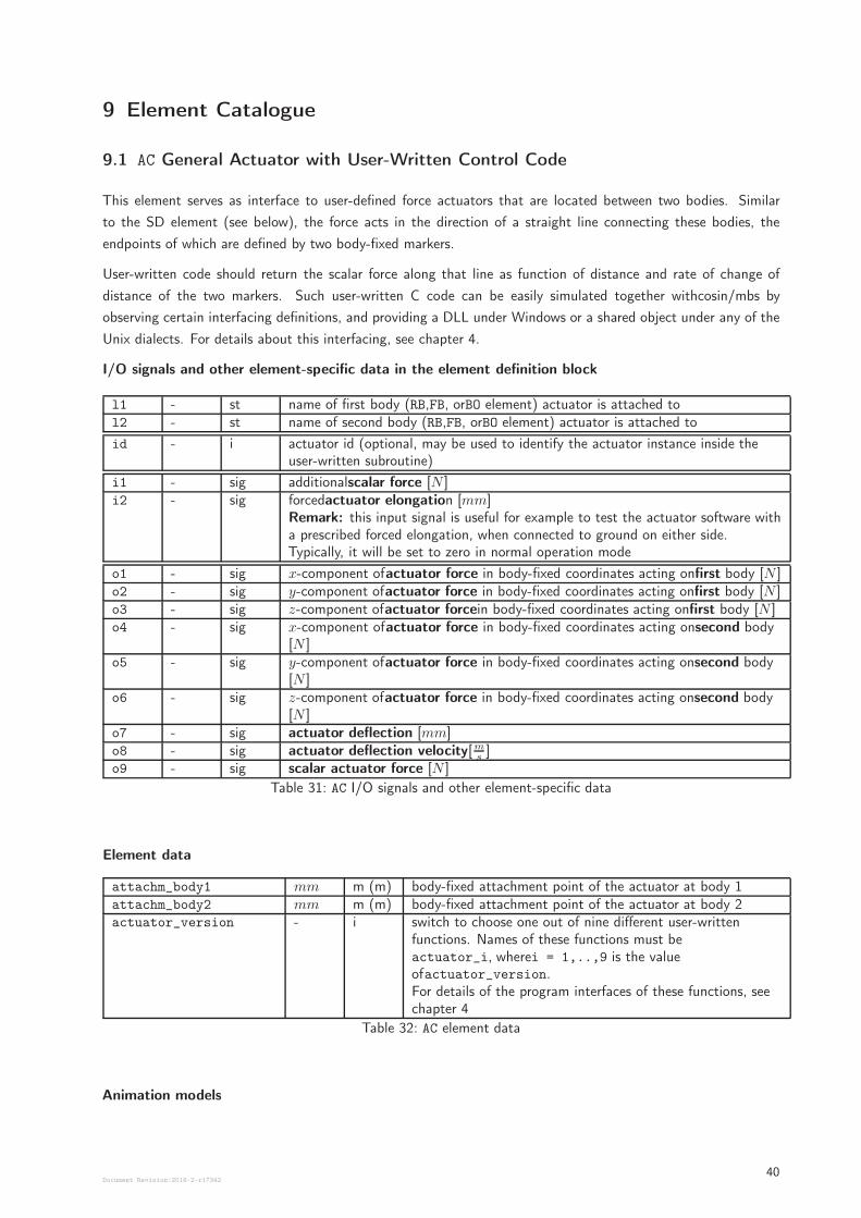
9 Element Catalogue
9.1 AC General Actuator with User-Written Control Code
This element serves as interface to user-defined force actuators that are located between two bodies. Similar
to the SD element (see below), the force acts in the direction of a straight line connecting these bodies, the
endpoints of which are defined by two body-fixed markers.
User-written code should return the scalar force along that line as function of distance and rate of change of
distance of the two markers. Such user-written C code can be easily simulated together withcosin/mbs by
observing certain interfacing definitions, and providing a DLL under Windows or a shared object under any of the
Unix dialects. For details about this interfacing, see chapter 4.
I/O signals and other element-specific data in the element definition block
l1 - st name of first body (RB,FB, orBO element) actuator is attached tol2 - st name of second body (RB,FB, orBO element) actuator is attached to
id - i actuator id (optional, may be used to identify the actuator instance inside theuser-written subroutine)
i1 - sig additionalscalar force [N ]i2 - sig forcedactuator elongation [mm]
Remark: this input signal is useful for example to test the actuator software witha prescribed forced elongation, when connected to ground on either side.Typically, it will be set to zero in normal operation mode
o1 - sig x-component ofactuator force in body-fixed coordinates acting onfirst body [N ]o2 - sig y-component ofactuator force in body-fixed coordinates acting onfirst body [N ]o3 - sig z-component ofactuator forcein body-fixed coordinates acting onfirst body [N ]o4 - sig x-component ofactuator force in body-fixed coordinates acting onsecond body
[N ]o5 - sig y-component ofactuator force in body-fixed coordinates acting onsecond body
[N ]o6 - sig z-component ofactuator force in body-fixed coordinates acting onsecond body
[N ]o7 - sig actuator deflection [mm]o8 - sig actuator deflection velocity[m
s]
o9 - sig scalar actuator force [N ]
Table 31: AC I/O signals and other element-specific data
Element data
attachm_body1 mm m (m) body-fixed attachment point of the actuator at body 1attachm_body2 mm m (m) body-fixed attachment point of the actuator at body 2actuator_version - i switch to choose one out of nine different user-written
functions. Names of these functions must beactuator_i, wherei = 1,..,9 is the valueofactuator_version.For details of the program interfaces of these functions, seechapter 4
Table 32: AC element data
Animation models
Document Revision:2018-2-r1734240
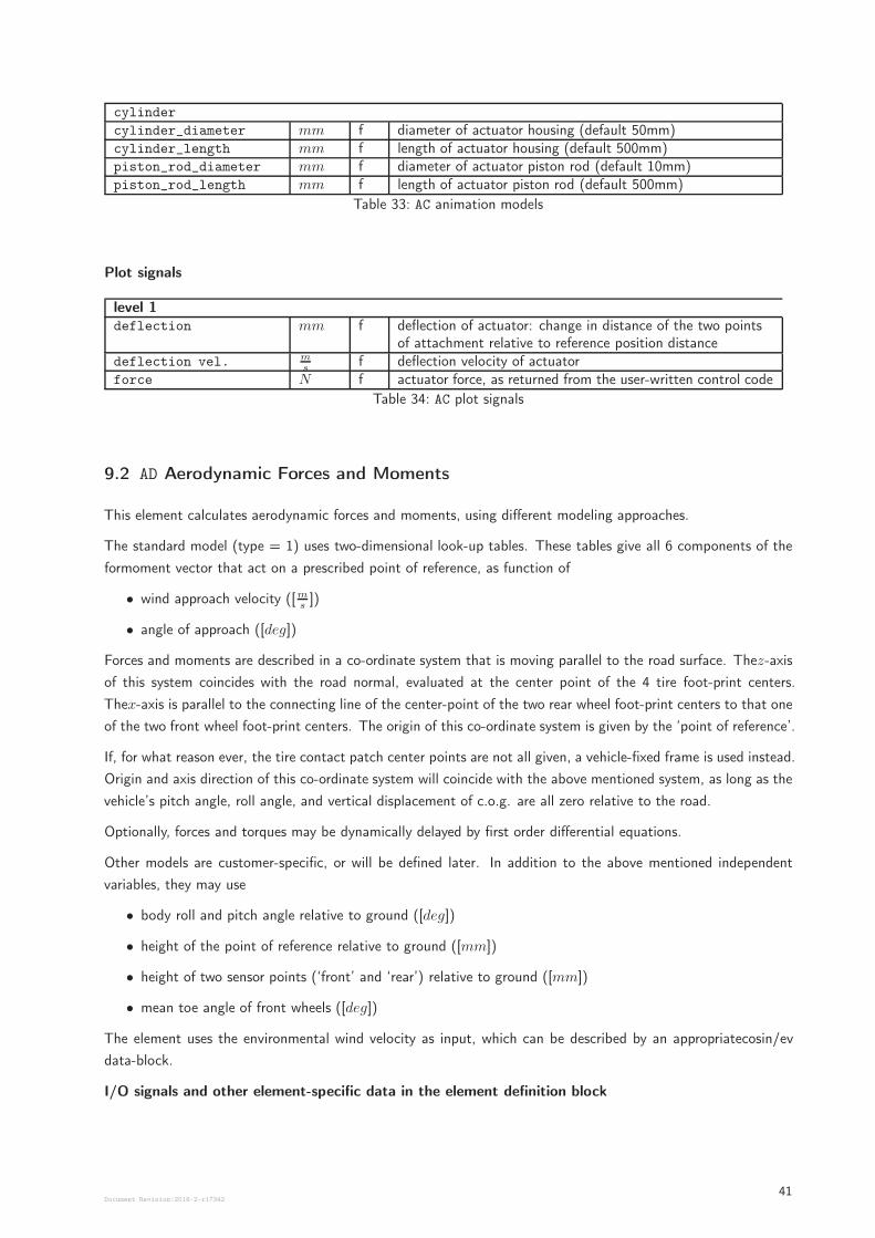
cylinder
cylinder_diameter mm f diameter of actuator housing (default 50mm)cylinder_length mm f length of actuator housing (default 500mm)piston_rod_diameter mm f diameter of actuator piston rod (default 10mm)piston_rod_length mm f length of actuator piston rod (default 500mm)
Table 33: AC animation models
Plot signals
level 1deflection mm f deflection of actuator: change in distance of the two points
of attachment relative to reference position distancedeflection vel. m
sf deflection velocity of actuator
force N f actuator force, as returned from the user-written control code
Table 34: AC plot signals
9.2 AD Aerodynamic Forces and Moments
This element calculates aerodynamic forces and moments, using different modeling approaches.
The standard model (type = 1) uses two-dimensional look-up tables. These tables give all 6 components of the
formoment vector that act on a prescribed point of reference, as function of
• wind approach velocity ([ms])
• angle of approach ([deg])
Forces and moments are described in a co-ordinate system that is moving parallel to the road surface. Thez-axis
of this system coincides with the road normal, evaluated at the center point of the 4 tire foot-print centers.
Thex-axis is parallel to the connecting line of the center-point of the two rear wheel foot-print centers to that one
of the two front wheel foot-print centers. The origin of this co-ordinate system is given by the ‘point of reference’.
If, for what reason ever, the tire contact patch center points are not all given, a vehicle-fixed frame is used instead.
Origin and axis direction of this co-ordinate system will coincide with the above mentioned system, as long as the
vehicle’s pitch angle, roll angle, and vertical displacement of c.o.g. are all zero relative to the road.
Optionally, forces and torques may be dynamically delayed by first order differential equations.
Other models are customer-specific, or will be defined later. In addition to the above mentioned independent
variables, they may use
• body roll and pitch angle relative to ground ([deg])
• height of the point of reference relative to ground ([mm])
• height of two sensor points (‘front’ and ‘rear’) relative to ground ([mm])
• mean toe angle of front wheels ([deg])
The element uses the environmental wind velocity as input, which can be described by an appropriatecosin/ev
data-block.
I/O signals and other element-specific data in the element definition block
Document Revision:2018-2-r1734241
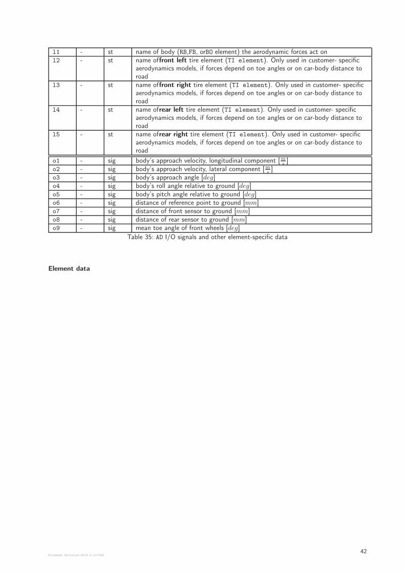
l1 - st name of body (RB,FB, orBO element) the aerodynamic forces act onl2 - st name offront left tire element (TI element). Only used in customer- specific
aerodynamics models, if forces depend on toe angles or on car-body distance toroad
l3 - st name offront right tire element (TI element). Only used in customer- specificaerodynamics models, if forces depend on toe angles or on car-body distance toroad
l4 - st name ofrear left tire element (TI element). Only used in customer- specificaerodynamics models, if forces depend on toe angles or on car-body distance toroad
l5 - st name ofrear right tire element (TI element). Only used in customer- specificaerodynamics models, if forces depend on toe angles or on car-body distance toroad
o1 - sig body’s approach velocity, longitudinal component [ms]
o2 - sig body’s approach velocity, lateral component [ms]
o3 - sig body’s approach angle [deg]o4 - sig body’s roll angle relative to ground [deg]o5 - sig body’s pitch angle relative to ground [deg]o6 - sig distance of reference point to ground [mm]o7 - sig distance of front sensor to ground [mm]o8 - sig distance of rear sensor to ground [mm]o9 - sig mean toe angle of front wheels [deg]
Table 35: AD I/O signals and other element-specific data
Element data
Document Revision:2018-2-r1734242
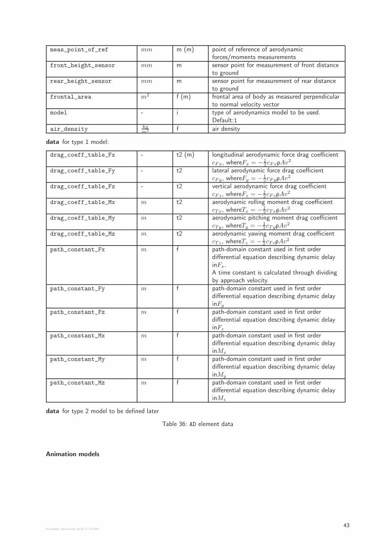
meas_point_of_ref mm m (m) point of reference of aerodynamicforces/moments measurements
front_height_sensor mm m sensor point for measurement of front distanceto ground
rear_height_sensor mm m sensor point for measurement of rear distanceto ground
frontal_area m2 f (m) frontal area of body as measured perpendicularto normal velocity vector
model - i type of aerodynamics model to be used.Default:1
air_density kgm3 f air density
data for type 1 model:
drag_coeff_table_Fx - t2 (m) longitudinal aerodynamic force drag coefficientcFx, whereFx = −
1
2cFxρAv
2
drag_coeff_table_Fy - t2 lateral aerodynamic force drag coefficientcFy, whereFy = −
1
2cFyρAv
2
drag_coeff_table_Fz - t2 vertical aerodynamic force drag coefficientcFz, whereFz = −
1
2cFzρAv
2
drag_coeff_table_Mx m t2 aerodynamic rolling moment drag coefficientcTx, whereTx = − 1
2cTxρAv
2
drag_coeff_table_My m t2 aerodynamic pitching moment drag coefficientcTy, whereTy = −
1
2cTyρAv
2
drag_coeff_table_Mz m t2 aerodynamic yawing moment drag coefficientcTz , whereTz = − 1
2cTzρAv
2
path_constant_Fx m f path-domain constant used in first orderdifferential equation describing dynamic delayinFx.A time constant is calculated through dividingby approach velocity.
path_constant_Fy m f path-domain constant used in first orderdifferential equation describing dynamic delayinFy
path_constant_Fz m f path-domain constant used in first orderdifferential equation describing dynamic delayinFz
path_constant_Mx m f path-domain constant used in first orderdifferential equation describing dynamic delayinMx
path_constant_My m f path-domain constant used in first orderdifferential equation describing dynamic delayinMy
path_constant_Mz m f path-domain constant used in first orderdifferential equation describing dynamic delayinMz
data for type 2 model to be defined later
Table 36: AD element data
Animation models
Document Revision:2018-2-r1734243
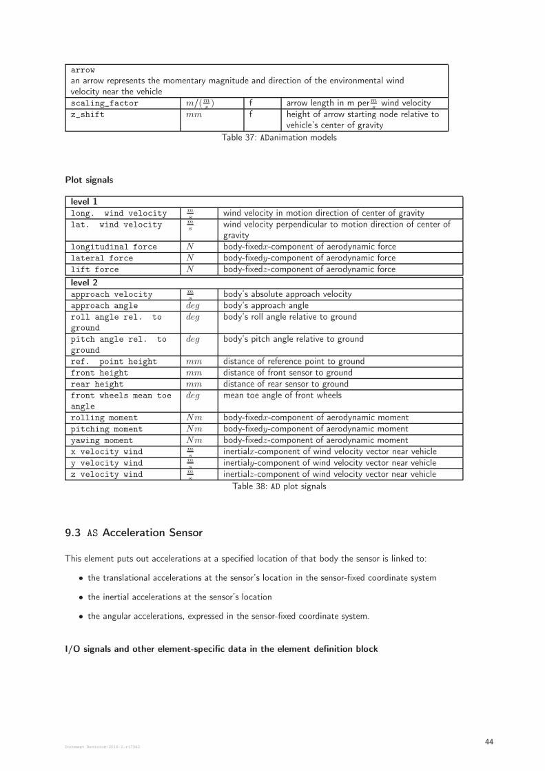
arrow
an arrow represents the momentary magnitude and direction of the environmental windvelocity near the vehiclescaling_factor m/(m
s) f arrow length in m perm
swind velocity
z_shift mm f height of arrow starting node relative tovehicle’s center of gravity
Table 37: ADanimation models
Plot signals
level 1long. wind velocity m
swind velocity in motion direction of center of gravity
lat. wind velocity ms
wind velocity perpendicular to motion direction of center ofgravity
longitudinal force N body-fixedx-component of aerodynamic forcelateral force N body-fixedy-component of aerodynamic forcelift force N body-fixedz-component of aerodynamic force
level 2approach velocity m
sbody’s absolute approach velocity
approach angle deg body’s approach angleroll angle rel. to
ground
deg body’s roll angle relative to ground
pitch angle rel. to
ground
deg body’s pitch angle relative to ground
ref. point height mm distance of reference point to groundfront height mm distance of front sensor to groundrear height mm distance of rear sensor to groundfront wheels mean toe
angle
deg mean toe angle of front wheels
rolling moment Nm body-fixedx-component of aerodynamic momentpitching moment Nm body-fixedy-component of aerodynamic momentyawing moment Nm body-fixedz-component of aerodynamic momentx velocity wind m
sinertialx-component of wind velocity vector near vehicle
y velocity wind ms
inertialy-component of wind velocity vector near vehiclez velocity wind m
sinertialz-component of wind velocity vector near vehicle
Table 38: AD plot signals
9.3 AS Acceleration Sensor
This element puts out accelerations at a specified location of that body the sensor is linked to:
• the translational accelerations at the sensor’s location in the sensor-fixed coordinate system
• the inertial accelerations at the sensor’s location
• the angular accelerations, expressed in the sensor-fixed coordinate system.
I/O signals and other element-specific data in the element definition block
Document Revision:2018-2-r1734244
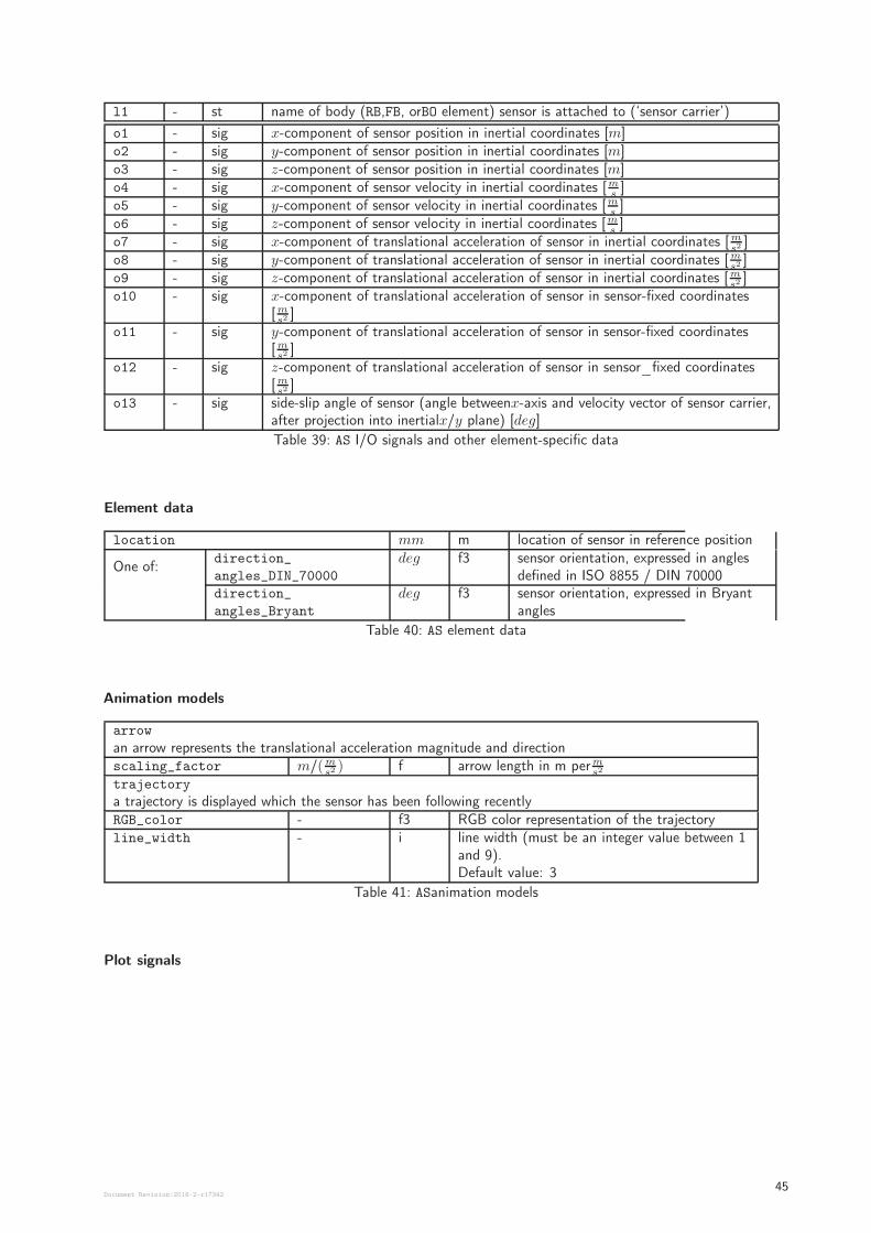
l1 - st name of body (RB,FB, orBO element) sensor is attached to (‘sensor carrier’)
o1 - sig x-component of sensor position in inertial coordinates [m]o2 - sig y-component of sensor position in inertial coordinates [m]o3 - sig z-component of sensor position in inertial coordinates [m]o4 - sig x-component of sensor velocity in inertial coordinates [m
s]
o5 - sig y-component of sensor velocity in inertial coordinates [ms]
o6 - sig z-component of sensor velocity in inertial coordinates [ms]
o7 - sig x-component of translational acceleration of sensor in inertial coordinates [ms2
]o8 - sig y-component of translational acceleration of sensor in inertial coordinates [m
s2]
o9 - sig z-component of translational acceleration of sensor in inertial coordinates [ms2
]o10 - sig x-component of translational acceleration of sensor in sensor-fixed coordinates
[ms2
]o11 - sig y-component of translational acceleration of sensor in sensor-fixed coordinates
[ms2
]o12 - sig z-component of translational acceleration of sensor in sensor_fixed coordinates
[ms2
]o13 - sig side-slip angle of sensor (angle betweenx-axis and velocity vector of sensor carrier,
after projection into inertialx/y plane) [deg]
Table 39: AS I/O signals and other element-specific data
Element data
location mm m location of sensor in reference position
One of:direction_
angles_DIN_70000
deg f3 sensor orientation, expressed in anglesdefined in ISO 8855 / DIN 70000
direction_
angles_Bryant
deg f3 sensor orientation, expressed in Bryantangles
Table 40: AS element data
Animation models
arrow
an arrow represents the translational acceleration magnitude and directionscaling_factor m/(m
s2) f arrow length in m perm
s2
trajectory
a trajectory is displayed which the sensor has been following recentlyRGB_color - f3 RGB color representation of the trajectoryline_width - i line width (must be an integer value between 1
and 9).Default value: 3
Table 41: ASanimation models
Plot signals
Document Revision:2018-2-r1734245
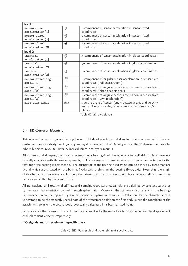
level 1sensor-fixed
acceleration[1]
ms2
x-component of sensor acceleration in sensor- fixedcoordinates
sensor-fixed
acceleration[2]
ms2
y-component of sensor acceleration in sensor- fixedcoordinates
sensor-fixed
acceleration[3]
ms2
z-component of sensor acceleration in sensor- fixedcoordinates
level 2inertial
acceleration[1]
ms2
x-component of sensor acceleration in global coordinates
inertial
acceleration[2]
ms2
y-component of sensor acceleration in global coordinates
inertial
acceleration[3]
ms2
z-component of sensor acceleration in global coordinates
sensor-fixed ang.
accel.[1]
degs2
x-component of angular sensor acceleration in sensor-fixedcoordinates (‘roll acceleration’)
sensor-fixed ang.
accel.[2]
degs2
y-component of angular sensor acceleration in sensor-fixedcoordinates (‘pitch acceleration’)
sensor-fixed ang.
accel.[3]
degs2
z-component of angular sensor acceleration in sensor-fixedcoordinates (‘yaw acceleration’)
side-slip angle deg side-slip angle of sensor (angle betweenx-axis and velocityvector of sensor carrier, after projection into inertialx/yplane)
Table 42: AS plot signals
9.4 BE General Bearing
This element serves as general description of all kinds of elasticity and damping that can assumed to be con-
centrated in one elasticity point, joining two rigid or flexible bodies. Among others, theBE element can describe
rubber bushings, revolute joints, cylindrical joints, and hydro-mounts.
All stiffness and damping data are understood in a bearing-fixed frame, where for cylindrical joints thex-axis
typically coincides with the axis of symmetry. This bearing-fixed frame is assumed to move and rotate with the
first body, the bearing is attached to. The orientation of the bearing-fixed frame can be defined by three markers,
two of which are situated on the bearing-fixedx-axis, a third on the bearing-fixedy-axis. Note that the origin
of this frame is of no relevance, but only the orientation. For this reason, nothing changes if all of these three
markers are shifted by the same vector.
All translational and rotational stiffness and damping characteristics can either be defined by constant values, or
by nonlinear characteristics, defined through spline data. Moreover, the stiffness characteristic in the bearing-
fixedx-direction can be replaced by a one-dimensional hydro-mount model. ‘Deflection’ for the characteristics is
understood to be the respective coordinate of the attachment point on the first body minus the coordinate of the
attachment point on the second body, eventually calculated in a bearing-fixed frame.
Signs are such that forces or moments normally share it with the respective translational or angular displacement
or displacement velocity, respectively.
I/O signals and other element-specific data
Table 43: BE I/O signals and other element-specific data
Document Revision:2018-2-r1734246
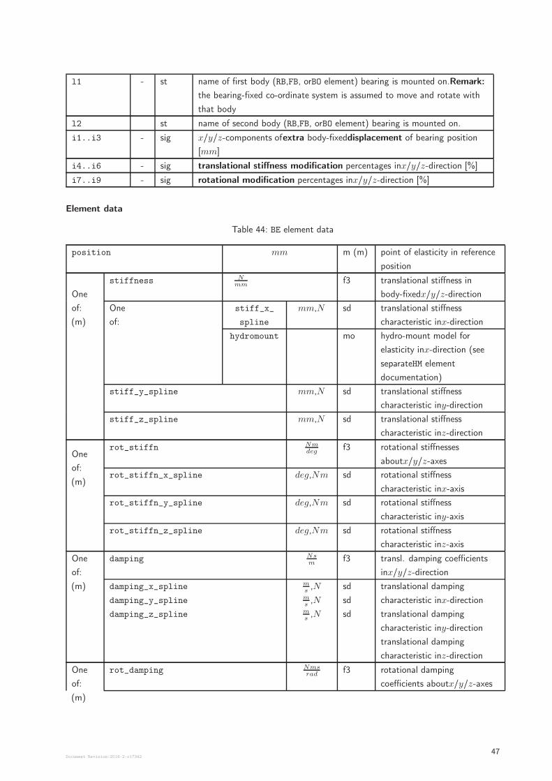
l1 - st name of first body (RB,FB, orBO element) bearing is mounted on.Remark:
the bearing-fixed co-ordinate system is assumed to move and rotate with
that body
l2 st name of second body (RB,FB, orBO element) bearing is mounted on.
i1..i3 - sig x/y/z-components ofextra body-fixeddisplacement of bearing position
[mm]
i4..i6 - sig translational stiffness modification percentages inx/y/z-direction [%]
i7..i9 - sig rotational modification percentages inx/y/z-direction [%]
Element data
Table 44: BE element data
position mm m (m) point of elasticity in reference
position
One
of:
(m)
stiffness Nmm
f3 translational stiffness in
body-fixedx/y/z-direction
One
of:
stiff_x_
spline
mm,N sd translational stiffness
characteristic inx-direction
hydromount mo hydro-mount model for
elasticity inx-direction (see
separateHM element
documentation)
stiff_y_spline mm,N sd translational stiffness
characteristic iny-direction
stiff_z_spline mm,N sd translational stiffness
characteristic inz-direction
One
of:
(m)
rot_stiffn Nmdeg
f3 rotational stiffnesses
aboutx/y/z-axes
rot_stiffn_x_spline deg,Nm sd rotational stiffness
characteristic inx-axis
rot_stiffn_y_spline deg,Nm sd rotational stiffness
characteristic iny-axis
rot_stiffn_z_spline deg,Nm sd rotational stiffness
characteristic inz-axis
One
of:
(m)
damping Nsm
f3 transl. damping coefficients
inx/y/z-direction
damping_x_spline
damping_y_spline
damping_z_spline
ms,N
ms,N
ms,N
sd
sd
sd
translational damping
characteristic inx-direction
translational damping
characteristic iny-direction
translational damping
characteristic inz-direction
One
of:
(m)
rot_damping Nmsrad
f3 rotational damping
coefficients aboutx/y/z-axes
Document Revision:2018-2-r1734247
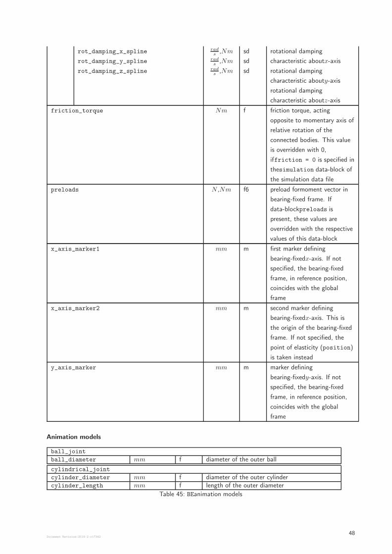
rot_damping_x_spline
rot_damping_y_spline
rot_damping_z_spline
rads
,Nmrads
,Nmrads
,Nm
sd
sd
sd
rotational damping
characteristic aboutx-axis
rotational damping
characteristic abouty-axis
rotational damping
characteristic aboutz-axis
friction_torque Nm f friction torque, acting
opposite to momentary axis of
relative rotation of the
connected bodies. This value
is overridden with 0,
iffriction = 0 is specified in
thesimulation data-block of
the simulation data file
preloads N ,Nm f6 preload formoment vector in
bearing-fixed frame. If
data-blockpreloads is
present, these values are
overridden with the respective
values of this data-block
x_axis_marker1 mm m first marker defining
bearing-fixedx-axis. If not
specified, the bearing-fixed
frame, in reference position,
coincides with the global
frame
x_axis_marker2 mm m second marker defining
bearing-fixedx-axis. This is
the origin of the bearing-fixed
frame. If not specified, the
point of elasticity (position)
is taken instead
y_axis_marker mm m marker defining
bearing-fixedy-axis. If not
specified, the bearing-fixed
frame, in reference position,
coincides with the global
frame
Animation models
ball_joint
ball_diameter mm f diameter of the outer ball
cylindrical_joint
cylinder_diameter mm f diameter of the outer cylindercylinder_length mm f length of the outer diameter
Table 45: BEanimation models
Document Revision:2018-2-r1734248
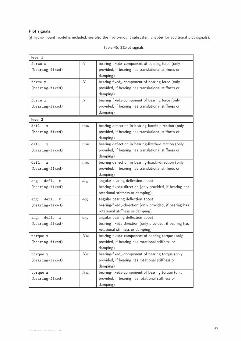
Plot signals
(if hydro-mount model is included, see also the hydro-mount subsystem chapter for additional plot signals):
Table 46: BEplot signals
level 1
force x
(bearing-fixed)
N bearing fixedx-component of bearing force (only
provided, if bearing has translational stiffness or
damping)
force y
(bearing-fixed)
N bearing fixedy-component of bearing force (only
provided, if bearing has translational stiffness or
damping)
force z
(bearing-fixed)
N bearing fixedz-component of bearing force (only
provided, if bearing has translational stiffness or
damping)
level 2
defl. x
(bearing-fixed)
mm bearing deflection in bearing-fixedx-direction (only
provided, if bearing has translational stiffness or
damping)
defl. y
(bearing-fixed)
mm bearing deflection in bearing-fixedy-direction (only
provided, if bearing has translational stiffness or
damping)
defl. z
(bearing-fixed)
mm bearing deflection in bearing-fixedz-direction (only
provided, if bearing has translational stiffness or
damping)
ang. defl. x
(bearing-fixed)
deg angular bearing deflection about
bearing-fixedx-direction (only provided, if bearing has
rotational stiffness or damping)
ang. defl. y
(bearing-fixed)
deg angular bearing deflection about
bearing-fixedy-direction (only provided, if bearing has
rotational stiffness or damping)
ang. defl. z
(bearing-fixed)
deg angular bearing deflection about
bearing-fixedz-direction (only provided, if bearing has
rotational stiffness or damping)
torque x
(bearing-fixed)
Nm bearing-fixedx-component of bearing torque (only
provided, if bearing has rotational stiffness or
damping)
torque y
(bearing-fixed)
Nm bearing-fixedy-component of bearing torque (only
provided, if bearing has rotational stiffness or
damping)
torque z
(bearing-fixed)
Nm bearing-fixedz-component of bearing torque (only
provided, if bearing has rotational stiffness or
damping)
Document Revision:2018-2-r1734249
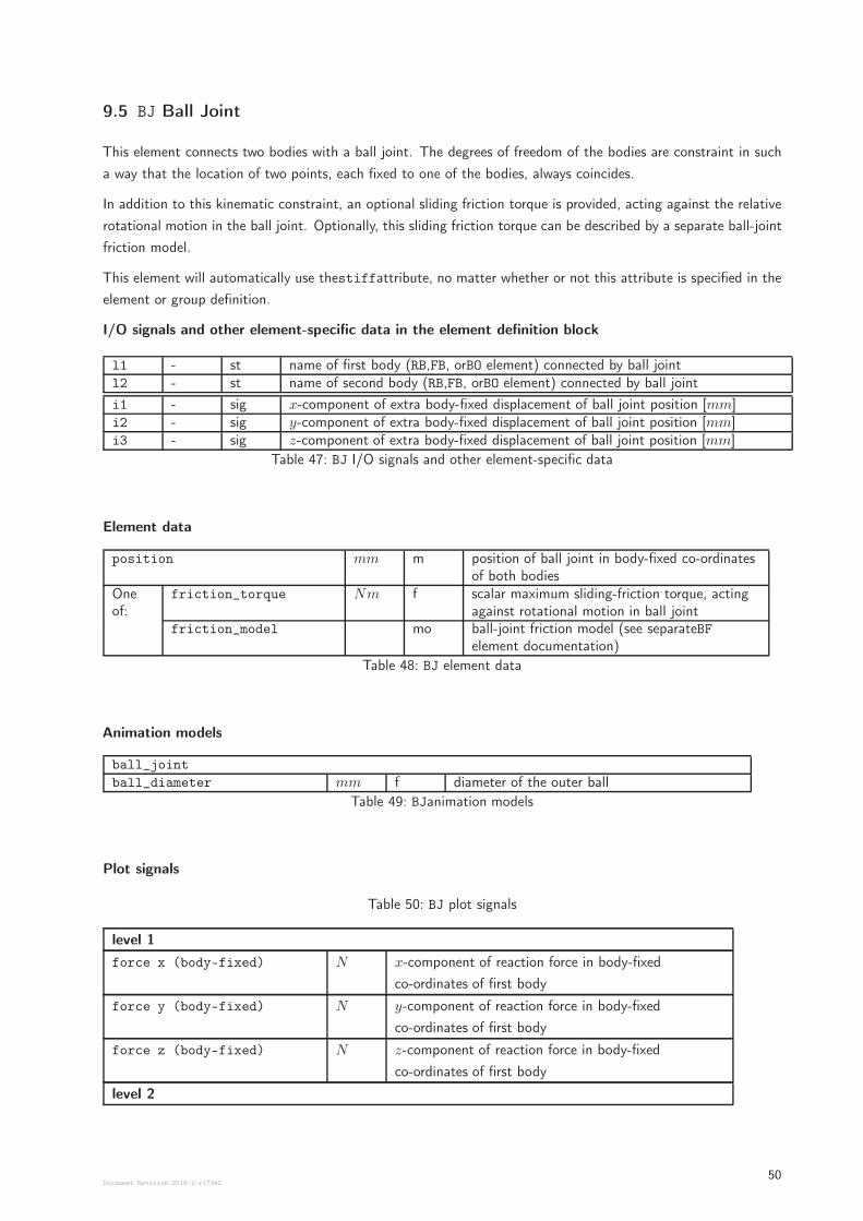
9.5 BJ Ball Joint
This element connects two bodies with a ball joint. The degrees of freedom of the bodies are constraint in such
a way that the location of two points, each fixed to one of the bodies, always coincides.
In addition to this kinematic constraint, an optional sliding friction torque is provided, acting against the relative
rotational motion in the ball joint. Optionally, this sliding friction torque can be described by a separate ball-joint
friction model.
This element will automatically use thestiffattribute, no matter whether or not this attribute is specified in the
element or group definition.
I/O signals and other element-specific data in the element definition block
l1 - st name of first body (RB,FB, orBO element) connected by ball jointl2 - st name of second body (RB,FB, orBO element) connected by ball joint
i1 - sig x-component of extra body-fixed displacement of ball joint position [mm]i2 - sig y-component of extra body-fixed displacement of ball joint position [mm]i3 - sig z-component of extra body-fixed displacement of ball joint position [mm]
Table 47: BJ I/O signals and other element-specific data
Element data
position mm m position of ball joint in body-fixed co-ordinatesof both bodies
Oneof:
friction_torque Nm f scalar maximum sliding-friction torque, actingagainst rotational motion in ball joint
friction_model mo ball-joint friction model (see separateBFelement documentation)
Table 48: BJ element data
Animation models
ball_joint
ball_diameter mm f diameter of the outer ball
Table 49: BJanimation models
Plot signals
Table 50: BJ plot signals
level 1
force x (body-fixed) N x-component of reaction force in body-fixed
co-ordinates of first body
force y (body-fixed) N y-component of reaction force in body-fixed
co-ordinates of first body
force z (body-fixed) N z-component of reaction force in body-fixed
co-ordinates of first body
level 2
Document Revision:2018-2-r1734250
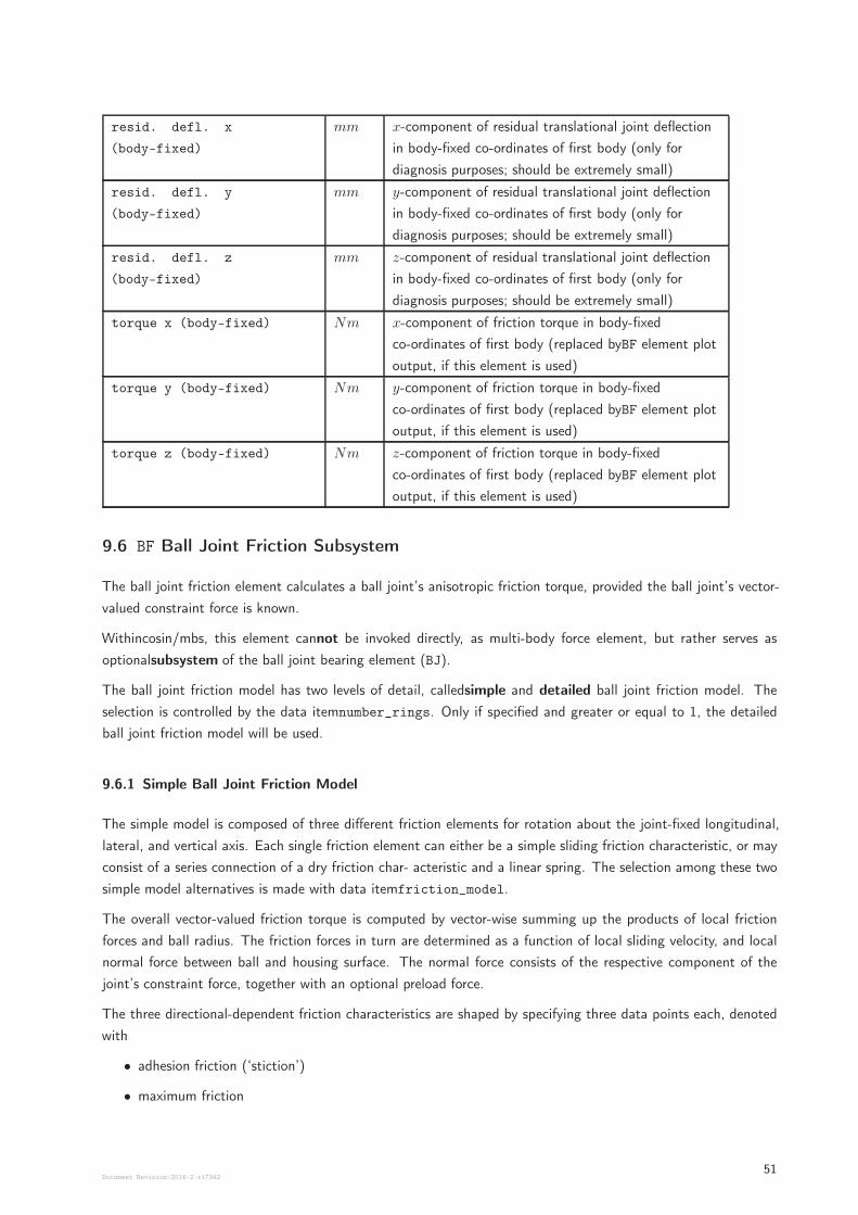
resid. defl. x
(body-fixed)
mm x-component of residual translational joint deflection
in body-fixed co-ordinates of first body (only for
diagnosis purposes; should be extremely small)
resid. defl. y
(body-fixed)
mm y-component of residual translational joint deflection
in body-fixed co-ordinates of first body (only for
diagnosis purposes; should be extremely small)
resid. defl. z
(body-fixed)
mm z-component of residual translational joint deflection
in body-fixed co-ordinates of first body (only for
diagnosis purposes; should be extremely small)
torque x (body-fixed) Nm x-component of friction torque in body-fixed
co-ordinates of first body (replaced byBF element plot
output, if this element is used)
torque y (body-fixed) Nm y-component of friction torque in body-fixed
co-ordinates of first body (replaced byBF element plot
output, if this element is used)
torque z (body-fixed) Nm z-component of friction torque in body-fixed
co-ordinates of first body (replaced byBF element plot
output, if this element is used)
9.6 BF Ball Joint Friction Subsystem
The ball joint friction element calculates a ball joint’s anisotropic friction torque, provided the ball joint’s vector-
valued constraint force is known.
Withincosin/mbs, this element cannot be invoked directly, as multi-body force element, but rather serves as
optionalsubsystem of the ball joint bearing element (BJ).
The ball joint friction model has two levels of detail, calledsimple and detailed ball joint friction model. The
selection is controlled by the data itemnumber_rings. Only if specified and greater or equal to 1, the detailed
ball joint friction model will be used.
9.6.1 Simple Ball Joint Friction Model
The simple model is composed of three different friction elements for rotation about the joint-fixed longitudinal,
lateral, and vertical axis. Each single friction element can either be a simple sliding friction characteristic, or may
consist of a series connection of a dry friction char- acteristic and a linear spring. The selection among these two
simple model alternatives is made with data itemfriction_model.
The overall vector-valued friction torque is computed by vector-wise summing up the products of local friction
forces and ball radius. The friction forces in turn are determined as a function of local sliding velocity, and local
normal force between ball and housing surface. The normal force consists of the respective component of the
joint’s constraint force, together with an optional preload force.
The three directional-dependent friction characteristics are shaped by specifying three data points each, denoted
with
• adhesion friction (‘stiction’)
• maximum friction
Document Revision:2018-2-r1734251
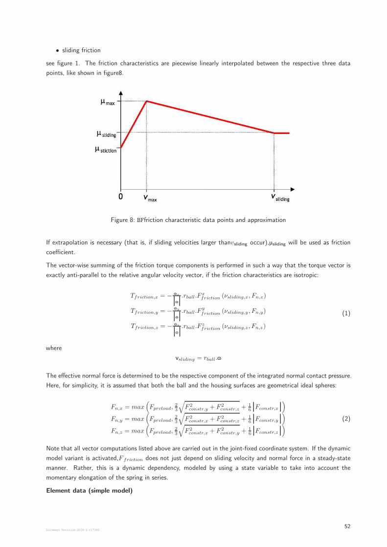
• sliding friction
see figure 1. The friction characteristics are piecewise linearly interpolated between the respective three data
points, like shown in figure8.
Figure 8: BFfriction characteristic data points and approximation
If extrapolation is necessary (that is, if sliding velocities larger thanvsliding occur),µsliding will be used as friction
coefficient.
The vector-wise summing of the friction torque components is performed in such a way that the torque vector is
exactly anti-parallel to the relative angular velocity vector, if the friction characteristics are isotropic:
Tfriction,x = −Ñx
Ñ
.rball.Fxfriction (νsliding,x, Fn,x)
Tfriction,y = −Ñy
Ñ
.rball.Fyfriction (νsliding,y , Fn,y)
Tfriction,z = −Ñz
Ñ
.rball.Fzfriction (νsliding,z , Fn,z)
(1)
where
νsliding = rball.Ñ
The effective normal force is determined to be the respective component of the integrated normal contact pressure.
Here, for simplicity, it is assumed that both the ball and the housing surfaces are geometrical ideal spheres:
Fn,x = max(
Fpreload,2
3
√
F 2constr,y + F 2
constr,z +1
6Fconstr,x
)
Fn,y = max(
Fpreload,2
3
√
F 2constr,x + F 2
constr,z +1
6Fconstr,y
)
Fn,z = max(
Fpreload,2
3
√
F 2constr,x + F 2
constr,y +1
6Fconstr,z
)
(2)
Note that all vector computations listed above are carried out in the joint-fixed coordinate system. If the dynamic
model variant is activated,F friction does not just depend on sliding velocity and normal force in a steady-state
manner. Rather, this is a dynamic dependency, modeled by using a state variable to take into account the
momentary elongation of the spring in series.
Element data (simple model)
Document Revision:2018-2-r1734252
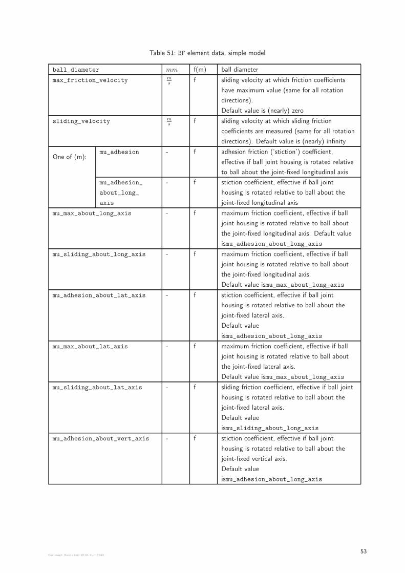
Table 51: BF element data, simple model
ball_diameter mm f(m) ball diameter
max_friction_velocity ms
f sliding velocity at which friction coefficients
have maximum value (same for all rotation
directions).
Default value is (nearly) zero
sliding_velocity ms
f sliding velocity at which sliding friction
coefficients are measured (same for all rotation
directions). Default value is (nearly) infinity
One of (m):mu_adhesion - f adhesion friction (‘stiction’) coefficient,
effective if ball joint housing is rotated relative
to ball about the joint-fixed longitudinal axis
mu_adhesion_
about_long_
axis
- f stiction coefficient, effective if ball joint
housing is rotated relative to ball about the
joint-fixed longitudinal axis
mu_max_about_long_axis - f maximum friction coefficient, effective if ball
joint housing is rotated relative to ball about
the joint-fixed longitudinal axis. Default value
ismu_adhesion_about_long_axis
mu_sliding_about_long_axis - f maximum friction coefficient, effective if ball
joint housing is rotated relative to ball about
the joint-fixed longitudinal axis.
Default value ismu_max_about_long_axis
mu_adhesion_about_lat_axis - f stiction coefficient, effective if ball joint
housing is rotated relative to ball about the
joint-fixed lateral axis.
Default value
ismu_adhesion_about_long_axis
mu_max_about_lat_axis - f maximum friction coefficient, effective if ball
joint housing is rotated relative to ball about
the joint-fixed lateral axis.
Default value ismu_max_about_long_axis
mu_sliding_about_lat_axis - f sliding friction coefficient, effective if ball joint
housing is rotated relative to ball about the
joint-fixed lateral axis.
Default value
ismu_sliding_about_long_axis
mu_adhesion_about_vert_axis - f stiction coefficient, effective if ball joint
housing is rotated relative to ball about the
joint-fixed vertical axis.
Default value
ismu_adhesion_about_long_axis
Document Revision:2018-2-r1734253
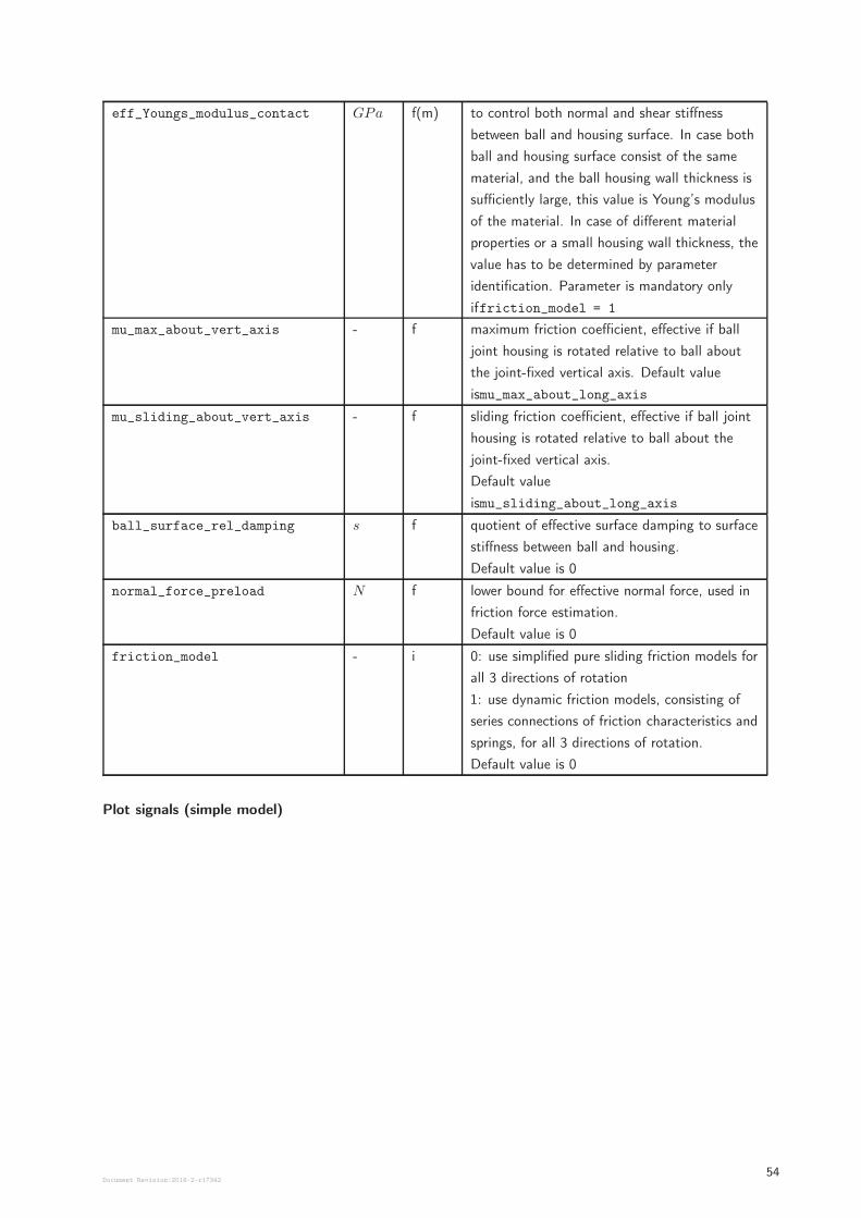
eff_Youngs_modulus_contact GPa f(m) to control both normal and shear stiffness
between ball and housing surface. In case both
ball and housing surface consist of the same
material, and the ball housing wall thickness is
sufficiently large, this value is Young’s modulus
of the material. In case of different material
properties or a small housing wall thickness, the
value has to be determined by parameter
identification. Parameter is mandatory only
iffriction_model = 1
mu_max_about_vert_axis - f maximum friction coefficient, effective if ball
joint housing is rotated relative to ball about
the joint-fixed vertical axis. Default value
ismu_max_about_long_axis
mu_sliding_about_vert_axis - f sliding friction coefficient, effective if ball joint
housing is rotated relative to ball about the
joint-fixed vertical axis.
Default value
ismu_sliding_about_long_axis
ball_surface_rel_damping s f quotient of effective surface damping to surface
stiffness between ball and housing.
Default value is 0
normal_force_preload N f lower bound for effective normal force, used in
friction force estimation.
Default value is 0
friction_model - i 0: use simplified pure sliding friction models for
all 3 directions of rotation
1: use dynamic friction models, consisting of
series connections of friction characteristics and
springs, for all 3 directions of rotation.
Default value is 0
Plot signals (simple model)
Document Revision:2018-2-r1734254
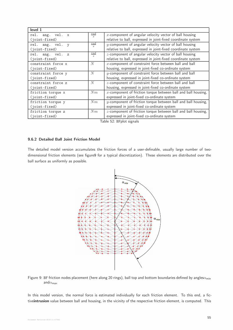
level 1
rel. ang. vel. x
(joint-fixed)
rads
x-component of angular velocity vector of ball housingrelative to ball, expressed in joint-fixed coordinate system
rel. ang. vel. y
(joint-fixed)
rads
y-component of angular velocity vector of ball housingrelative to ball, expressed in joint-fixed coordinate system
rel. ang. vel. z
(joint-fixed)
rads
z-component of angular velocity vector of ball housingrelative to ball, expressed in joint-fixed coordinate system
constraint force x
(joint-fixed)
N x-component of constraint force between ball and ballhousing, expressed in joint-fixed co-ordinate system
constraint force y
(joint-fixed)
N y-component of constraint force between ball and ballhousing, expressed in joint-fixed co-ordinate system
constraint force z
(joint-fixed)
N z-component of constraint force between ball and ballhousing, expressed in joint-fixed co-ordinate system
friction torque x
(joint-fixed)
Nm x-component of friction torque between ball and ball housing,expressed in joint-fixed co-ordinate system
friction torque y
(joint-fixed)
Nm y-component of friction torque between ball and ball housing,expressed in joint-fixed co-ordinate system
friction torque z
(joint-fixed)
Nm z-component of friction torque between ball and ball housing,expressed in joint-fixed co-ordinate system
Table 52: BFplot signals
9.6.2 Detailed Ball Joint Friction Model
The detailed model version accumulates the friction forces of a user-definable, usually large number of two-
dimensional friction elements (see figure9 for a typical discretization). These elements are distributed over the
ball surface as uniformly as possible.
Figure 9: BF friction nodes placement (here along 20 rings), ball top and bottom boundaries defined by anglesαmin
andαmax
In this model version, the normal force is estimated individually for each friction element. To this end, a fic-
tiveintrusion value between ball and housing, in the vicinity of the respective friction element, is computed. This
Document Revision:2018-2-r1734255
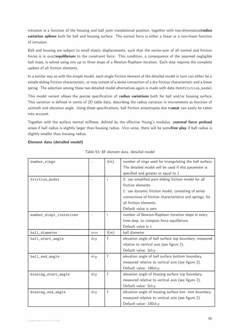
intrusion is a function of the housing and ball joint translational position, together with two-dimensionalradius
variation splines both for ball and housing surface. The normal force is either a linear or a non-linear function
of intrusion.
Ball and housing are subject to small elastic displacements, such that the vector-sum of all normal and friction
forces is in exactequilibrium to the constraint force. This condition, a consequence of the assumed negligible
ball mass, is solved using one up to three steps of a Newton-Raphson iteration. Each step requires the complete
update of all friction elements.
In a similar way as with the simple model, each single friction element of the detailed model in turn can either be a
simple sliding friction characteristic, or may consist of a series connection of a dry friction characteristic and a linear
spring. The selection among these two detailed model alternatives again is made with data itemfriction_model.
This model variant allows the precise specification of radius variations both for ball and/or housing surface.
This variation is defined in terms of 2D table data, describing the radius variation in micrometers as function of
azimuth and elevation angle. Using these specifications, ball friction anisotropies due towear can easily be taken
into account.
Together with the surface normal stiffness, defined by the effective Young’s modulus, anormal force preload
arises if ball radius is slightly larger than housing radius. Vice versa, there will be somefree play if ball radius is
slightly smaller than housing radius.
Element data (detailed model)
Table 53: BF element data, detailed model
number_rings - i(m) number of rings used for triangulating the ball surface.
The detailed model will be used if this parameter is
specified and greater or equal to 1
friction_model - i 0: use simplified pure sliding friction model for all
friction elements
1: use dynamic friction model, consisting of series
connections of friction characteristics and springs, for
all friction elements.
Default value is zero
number_displ_iterations - i number of Newton-Raphson iteration steps in every
time step, to compute force equilibrium.
Default value is 1
ball_diameter mm f(m) ball diameter
ball_start_angle deg f elevation angle of ball surface top boundary, measured
relative to vertical axis (see figure 2).
Default value: 0deg
ball_end_angle deg f elevation angle of ball surface bottom boundary,
measured relative to vertical axis (see figure 2).
Default value: 180deg
housing_start_angle deg f elevation angle of housing surface top boundary,
measured relative to vertical axis (see figure 2).
Default value: 0deg
housing_end_angle deg f elevation angle of housing surface bot- tom boundary,
measured relative to vertical axis (see figure 2).
Default value: 180deg
Document Revision:2018-2-r1734256
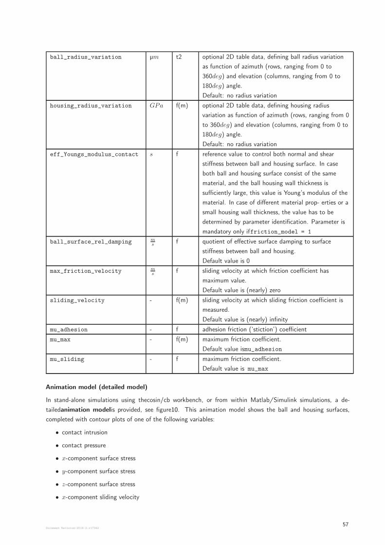
ball_radius_variation µm t2 optional 2D table data, defining ball radius variation
as function of azimuth (rows, ranging from 0 to
360deg) and elevation (columns, ranging from 0 to
180deg) angle.
Default: no radius variation
housing_radius_variation GPa f(m) optional 2D table data, defining housing radius
variation as function of azimuth (rows, ranging from 0
to 360deg) and elevation (columns, ranging from 0 to
180deg) angle.
Default: no radius variation
eff_Youngs_modulus_contact s f reference value to control both normal and shear
stiffness between ball and housing surface. In case
both ball and housing surface consist of the same
material, and the ball housing wall thickness is
sufficiently large, this value is Young’s modulus of the
material. In case of different material prop- erties or a
small housing wall thickness, the value has to be
determined by parameter identification. Parameter is
mandatory only iffriction_model = 1
ball_surface_rel_damping ms
f quotient of effective surface damping to surface
stiffness between ball and housing.
Default value is 0
max_friction_velocity ms
f sliding velocity at which friction coefficient has
maximum value.
Default value is (nearly) zero
sliding_velocity - f(m) sliding velocity at which sliding friction coefficient is
measured.
Default value is (nearly) infinity
mu_adhesion - f adhesion friction (‘stiction’) coefficient
mu_max - f(m) maximum friction coefficient.
Default value ismu_adhesion
mu_sliding - f maximum friction coefficient.
Default value is mu_max
Animation model (detailed model)
In stand-alone simulations using thecosin/cb workbench, or from within Matlab/Simulink simulations, a de-
tailedanimation modelis provided, see figure10. This animation model shows the ball and housing surfaces,
completed with contour plots of one of the following variables:
• contact intrusion
• contact pressure
• x-component surface stress
• y-component surface stress
• z-component surface stress
• x-component sliding velocity
Document Revision:2018-2-r1734257
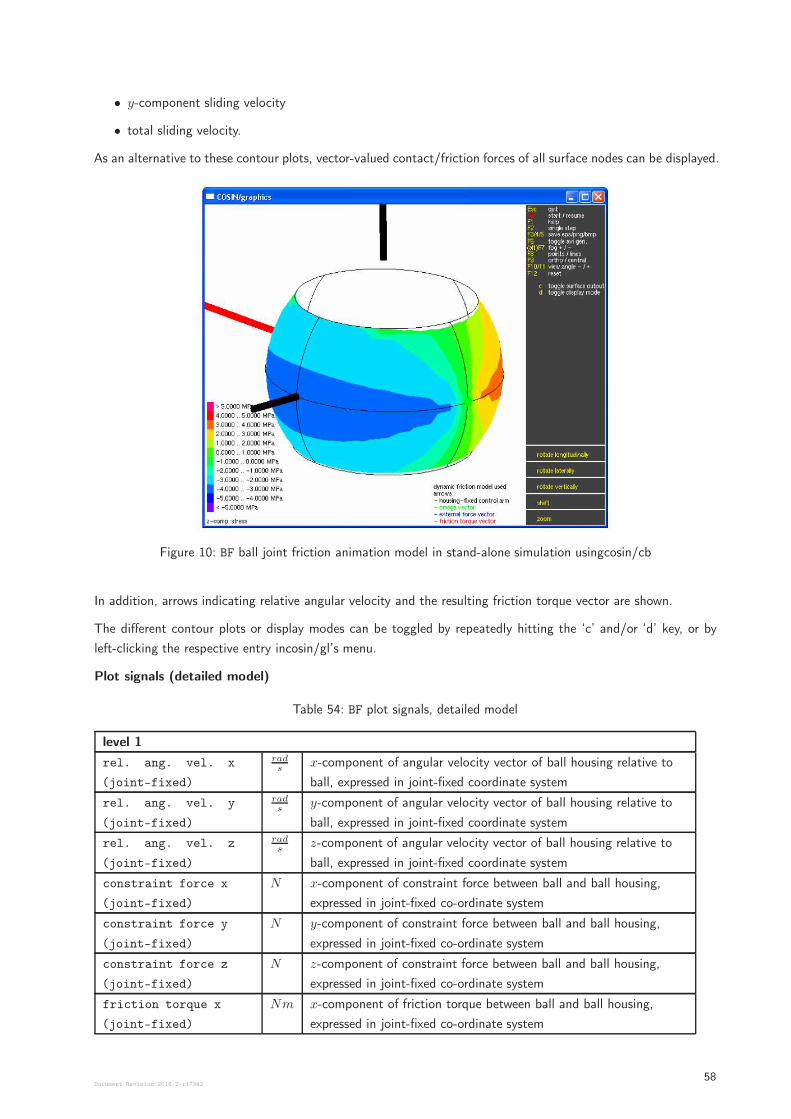
• y-component sliding velocity
• total sliding velocity.
As an alternative to these contour plots, vector-valued contact/friction forces of all surface nodes can be displayed.
Figure 10: BF ball joint friction animation model in stand-alone simulation usingcosin/cb
In addition, arrows indicating relative angular velocity and the resulting friction torque vector are shown.
The different contour plots or display modes can be toggled by repeatedly hitting the ‘c’ and/or ‘d’ key, or by
left-clicking the respective entry incosin/gl’s menu.
Plot signals (detailed model)
Table 54: BF plot signals, detailed model
level 1
rel. ang. vel. x
(joint-fixed)
rads
x-component of angular velocity vector of ball housing relative to
ball, expressed in joint-fixed coordinate system
rel. ang. vel. y
(joint-fixed)
rads
y-component of angular velocity vector of ball housing relative to
ball, expressed in joint-fixed coordinate system
rel. ang. vel. z
(joint-fixed)
rads
z-component of angular velocity vector of ball housing relative to
ball, expressed in joint-fixed coordinate system
constraint force x
(joint-fixed)
N x-component of constraint force between ball and ball housing,
expressed in joint-fixed co-ordinate system
constraint force y
(joint-fixed)
N y-component of constraint force between ball and ball housing,
expressed in joint-fixed co-ordinate system
constraint force z
(joint-fixed)
N z-component of constraint force between ball and ball housing,
expressed in joint-fixed co-ordinate system
friction torque x
(joint-fixed)
Nm x-component of friction torque between ball and ball housing,
expressed in joint-fixed co-ordinate system
Document Revision:2018-2-r1734258
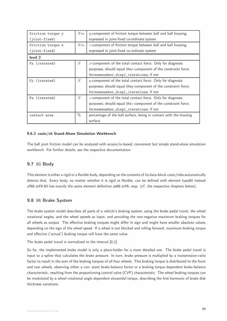
friction torque y
(joint-fixed)
Nm y-component of friction torque between ball and ball housing,
expressed in joint-fixed co-ordinate system
friction torque z
(joint-fixed)
Nm z-component of friction torque between ball and ball housing,
expressed in joint-fixed co-ordinate system
level 2
Fx (iterated) N x-component of the total contact force. Only for diagnosis
purposes; should equal thex-component of the constraint force.
Increasenumber_displ_iterations, if not
Fy (iterated) N y-component of the total contact force. Only for diagnosis
purposes; should equal they-component of the constraint force.
Increasenumber_displ_iterations, if not
Fz (iterated) N z-component of the total contact force. Only for diagnosis
purposes; should equal thez-component of the constraint force.
Increasenumber_displ_iterations, if not
contact area % percentage of the ball surface, being in contact with the housing
surface
9.6.3 cosin/cb Stand-Alone Simulation Workbench
The ball joint friction model can be analyzed with acosin/io-based, convenient but simple stand-alone simulation
workbench. For further details, see the respective documentation.
9.7 BO Body
This element is either a rigid or a flexible body, depending on the contents of its data-block.cosin/mbs automatically
detects that. Every body, no matter whether it is rigid or flexible, can be defined with element typeBO instead
ofRB orFB.BO has exactly the same element definition asRB orFB, resp. (cf. the respective chapters below).
9.8 BR Brake System
The brake system model describes all parts of a vehicle’s braking system, using the brake pedal travel, the wheel
rotational angles, and the wheel speeds as input, and providing the non-negative maximum braking torques for
all wheels as output. The effective braking torques might differ in sign and might have smaller absolute values,
depending on the sign of the wheel speed. If a wheel is not blocked and rolling forward, maximum braking torque
and effective (‘actual’) braking torque will have the same value.
The brake pedal travel is normalized to the interval [0,1].
So far, the implemented brake model is only a place-holder for a more detailed one. The brake pedal travel is
input to a spline that calculates the brake pressure. In turn, brake pressure is multiplied by a transmission-ratio
factor to result in the sum of the braking torques of all four wheels. This braking torque is distributed to the front
and rear wheels, observing either a con- stant brake-balance factor or a braking torque dependent brake-balance
characteristic, resulting from the proportioning control valve (CVP) characteristic. The wheel braking torques can
be modulated by a wheel rotational angle dependent sinusoidal torque, describing the first harmonic of brake disk
thickness variations.
Document Revision:2018-2-r1734259
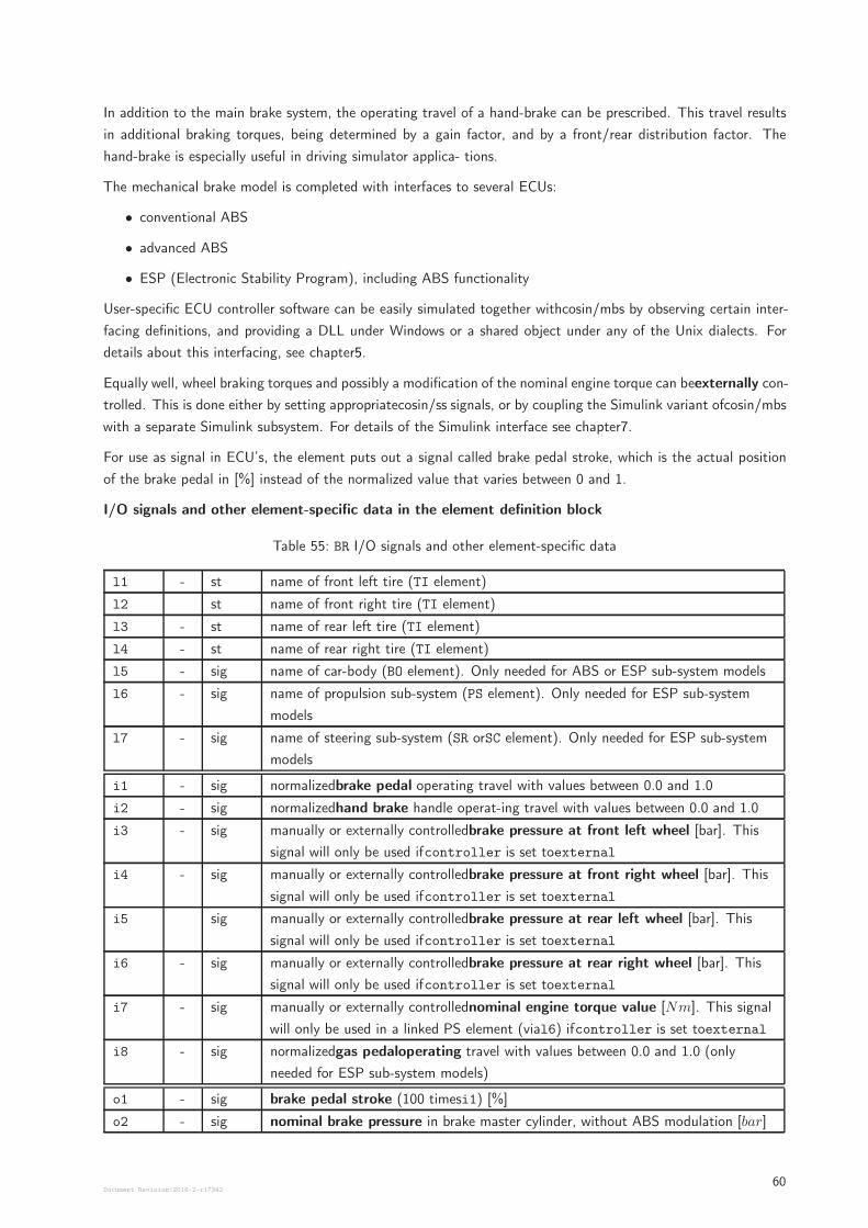
In addition to the main brake system, the operating travel of a hand-brake can be prescribed. This travel results
in additional braking torques, being determined by a gain factor, and by a front/rear distribution factor. The
hand-brake is especially useful in driving simulator applica- tions.
The mechanical brake model is completed with interfaces to several ECUs:
• conventional ABS
• advanced ABS
• ESP (Electronic Stability Program), including ABS functionality
User-specific ECU controller software can be easily simulated together withcosin/mbs by observing certain inter-
facing definitions, and providing a DLL under Windows or a shared object under any of the Unix dialects. For
details about this interfacing, see chapter5.
Equally well, wheel braking torques and possibly a modification of the nominal engine torque can beexternally con-
trolled. This is done either by setting appropriatecosin/ss signals, or by coupling the Simulink variant ofcosin/mbs
with a separate Simulink subsystem. For details of the Simulink interface see chapter7.
For use as signal in ECU’s, the element puts out a signal called brake pedal stroke, which is the actual position
of the brake pedal in [%] instead of the normalized value that varies between 0 and 1.
I/O signals and other element-specific data in the element definition block
Table 55: BR I/O signals and other element-specific data
l1 - st name of front left tire (TI element)
l2 st name of front right tire (TI element)
l3 - st name of rear left tire (TI element)
l4 - st name of rear right tire (TI element)
l5 - sig name of car-body (BO element). Only needed for ABS or ESP sub-system models
l6 - sig name of propulsion sub-system (PS element). Only needed for ESP sub-system
models
l7 - sig name of steering sub-system (SR orSC element). Only needed for ESP sub-system
models
i1 - sig normalizedbrake pedal operating travel with values between 0.0 and 1.0
i2 - sig normalizedhand brake handle operat-ing travel with values between 0.0 and 1.0
i3 - sig manually or externally controlledbrake pressure at front left wheel [bar]. This
signal will only be used ifcontroller is set toexternal
i4 - sig manually or externally controlledbrake pressure at front right wheel [bar]. This
signal will only be used ifcontroller is set toexternal
i5 sig manually or externally controlledbrake pressure at rear left wheel [bar]. This
signal will only be used ifcontroller is set toexternal
i6 - sig manually or externally controlledbrake pressure at rear right wheel [bar]. This
signal will only be used ifcontroller is set toexternal
i7 - sig manually or externally controllednominal engine torque value [Nm]. This signal
will only be used in a linked PS element (vial6) ifcontroller is set toexternal
i8 - sig normalizedgas pedaloperating travel with values between 0.0 and 1.0 (only
needed for ESP sub-system models)
o1 - sig brake pedal stroke (100 timesi1) [%]
o2 - sig nominal brake pressure in brake master cylinder, without ABS modulation [bar]
Document Revision:2018-2-r1734260
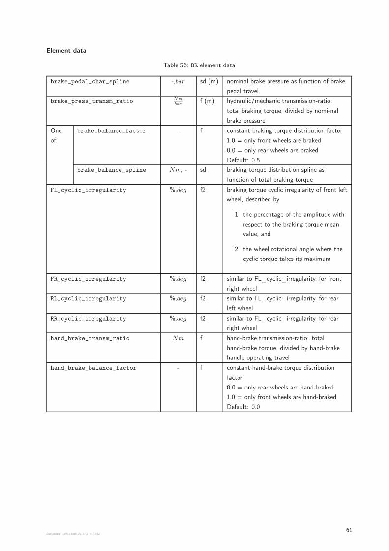
Element data
Table 56: BR element data
brake_pedal_char_spline -,bar sd (m) nominal brake pressure as function of brake
pedal travel
brake_press_transm_ratio Nmbar
f (m) hydraulic/mechanic transmission-ratio:
total braking torque, divided by nomi-nal
brake pressure
One
of:
brake_balance_factor - f constant braking torque distribution factor
1.0 = only front wheels are braked
0.0 = only rear wheels are braked
Default: 0.5
brake_balance_spline Nm, - sd braking torque distribution spline as
function of total braking torque
FL_cyclic_irregularity %,deg f2 braking torque cyclic irregularity of front left
wheel, described by
1. the percentage of the amplitude with
respect to the braking torque mean
value, and
2. the wheel rotational angle where the
cyclic torque takes its maximum
FR_cyclic_irregularity %,deg f2 similar to FL_cyclic_irregularity, for front
right wheel
RL_cyclic_irregularity %,deg f2 similar to FL_cyclic_irregularity, for rear
left wheel
RR_cyclic_irregularity %,deg f2 similar to FL_cyclic_irregularity, for rear
right wheel
hand_brake_transm_ratio Nm f hand-brake transmission-ratio: total
hand-brake torque, divided by hand-brake
handle operating travel
hand_brake_balance_factor - f constant hand-brake torque distribution
factor
0.0 = only rear wheels are hand-braked
1.0 = only front wheels are hand-braked
Default: 0.0
Document Revision:2018-2-r1734261
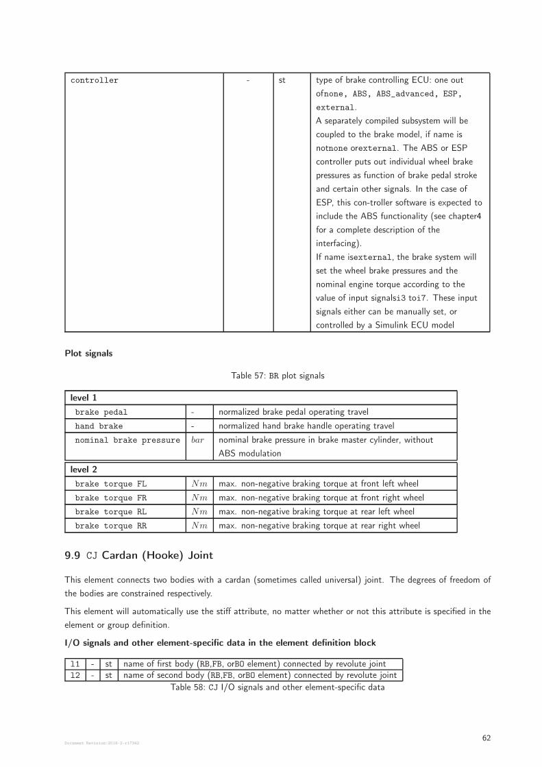
controller - st type of brake controlling ECU: one out
ofnone, ABS, ABS_advanced, ESP,
external.
A separately compiled subsystem will be
coupled to the brake model, if name is
notnone orexternal. The ABS or ESP
controller puts out individual wheel brake
pressures as function of brake pedal stroke
and certain other signals. In the case of
ESP, this con-troller software is expected to
include the ABS functionality (see chapter4
for a complete description of the
interfacing).
If name isexternal, the brake system will
set the wheel brake pressures and the
nominal engine torque according to the
value of input signalsi3 toi7. These input
signals either can be manually set, or
controlled by a Simulink ECU model
Plot signals
Table 57: BR plot signals
level 1
brake pedal - normalized brake pedal operating travel
hand brake - normalized hand brake handle operating travel
nominal brake pressure bar nominal brake pressure in brake master cylinder, without
ABS modulation
level 2
brake torque FL Nm max. non-negative braking torque at front left wheel
brake torque FR Nm max. non-negative braking torque at front right wheel
brake torque RL Nm max. non-negative braking torque at rear left wheel
brake torque RR Nm max. non-negative braking torque at rear right wheel
9.9 CJ Cardan (Hooke) Joint
This element connects two bodies with a cardan (sometimes called universal) joint. The degrees of freedom of
the bodies are constrained respectively.
This element will automatically use the stiff attribute, no matter whether or not this attribute is specified in the
element or group definition.
I/O signals and other element-specific data in the element definition block
l1 - st name of first body (RB,FB, orBO element) connected by revolute jointl2 - st name of second body (RB,FB, orBO element) connected by revolute joint
Table 58: CJ I/O signals and other element-specific data
Document Revision:2018-2-r1734262
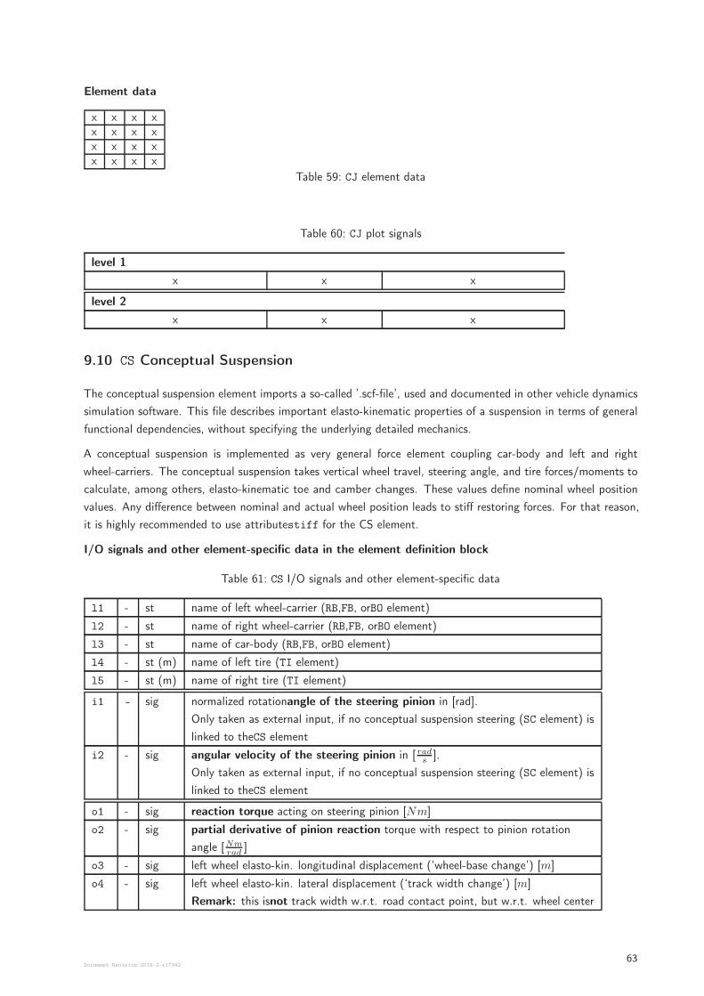
Element data
x x x xx x x xx x x xx x x x
Table 59: CJ element data
Table 60: CJ plot signals
level 1
x x x
level 2
x x x
9.10 CS Conceptual Suspension
The conceptual suspension element imports a so-called ’.scf-file’, used and documented in other vehicle dynamics
simulation software. This file describes important elasto-kinematic properties of a suspension in terms of general
functional dependencies, without specifying the underlying detailed mechanics.
A conceptual suspension is implemented as very general force element coupling car-body and left and right
wheel-carriers. The conceptual suspension takes vertical wheel travel, steering angle, and tire forces/moments to
calculate, among others, elasto-kinematic toe and camber changes. These values define nominal wheel position
values. Any difference between nominal and actual wheel position leads to stiff restoring forces. For that reason,
it is highly recommended to use attributestiff for the CS element.
I/O signals and other element-specific data in the element definition block
Table 61: CS I/O signals and other element-specific data
l1 - st name of left wheel-carrier (RB,FB, orBO element)
l2 - st name of right wheel-carrier (RB,FB, orBO element)
l3 - st name of car-body (RB,FB, orBO element)
l4 - st (m) name of left tire (TI element)
l5 - st (m) name of right tire (TI element)
i1 - sig normalized rotationangle of the steering pinion in [rad].
Only taken as external input, if no conceptual suspension steering (SC element) is
linked to theCS element
i2 - sig angular velocity of the steering pinion in [ rads
].
Only taken as external input, if no conceptual suspension steering (SC element) is
linked to theCS element
o1 - sig reaction torque acting on steering pinion [Nm]
o2 - sig partial derivative of pinion reaction torque with respect to pinion rotation
angle [Nmrad
]
o3 - sig left wheel elasto-kin. longitudinal displacement (‘wheel-base change’) [m]
o4 - sig left wheel elasto-kin. lateral displacement (‘track width change’) [m]
Remark: this isnot track width w.r.t. road contact point, but w.r.t. wheel center
Document Revision:2018-2-r1734263
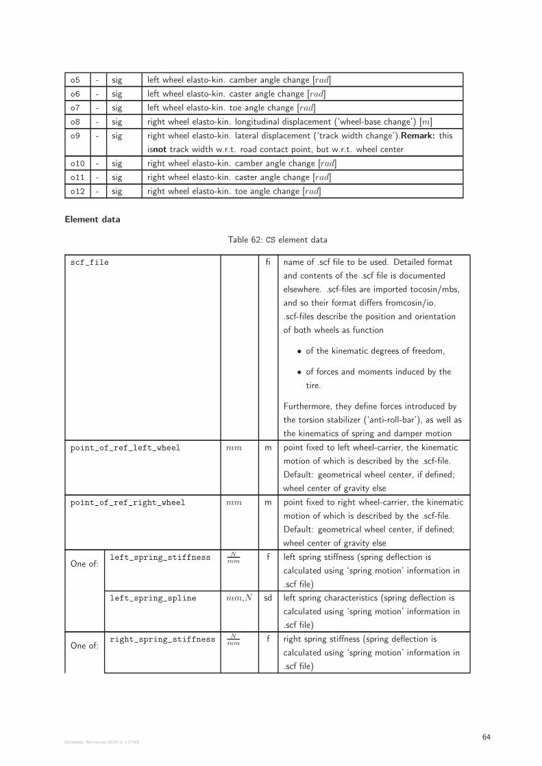
o5 - sig left wheel elasto-kin. camber angle change [rad]
o6 - sig left wheel elasto-kin. caster angle change [rad]
o7 - sig left wheel elasto-kin. toe angle change [rad]
o8 - sig right wheel elasto-kin. longitudinal displacement (‘wheel-base change’) [m]
o9 - sig right wheel elasto-kin. lateral displacement (‘track width change’).Remark: this
isnot track width w.r.t. road contact point, but w.r.t. wheel center
o10 - sig right wheel elasto-kin. camber angle change [rad]
o11 - sig right wheel elasto-kin. caster angle change [rad]
o12 - sig right wheel elasto-kin. toe angle change [rad]
Element data
Table 62: CS element data
scf_file fi name of .scf file to be used. Detailed format
and contents of the .scf file is documented
elsewhere. .scf-files are imported tocosin/mbs,
and so their format differs fromcosin/io.
.scf-files describe the position and orientation
of both wheels as function
• of the kinematic degrees of freedom,
• of forces and moments induced by the
tire.
Furthermore, they define forces introduced by
the torsion stabilizer (‘anti-roll-bar’), as well as
the kinematics of spring and damper motion
point_of_ref_left_wheel mm m point fixed to left wheel-carrier, the kinematic
motion of which is described by the .scf-file.
Default: geometrical wheel center, if defined;
wheel center of gravity else
point_of_ref_right_wheel mm m point fixed to right wheel-carrier, the kinematic
motion of which is described by the .scf-file.
Default: geometrical wheel center, if defined;
wheel center of gravity else
One of:left_spring_stiffness N
mmf left spring stiffness (spring deflection is
calculated using ‘spring motion’ information in
.scf file)
left_spring_spline mm,N sd left spring characteristics (spring deflection is
calculated using ‘spring motion’ information in
.scf file)
One of:right_spring_stiffness N
mmf right spring stiffness (spring deflection is
calculated using ‘spring motion’ information in
.scf file)
Document Revision:2018-2-r1734264
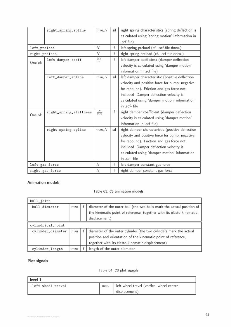
right_spring_spline mm,N sd right spring characteristics (spring deflection is
calculated using ‘spring motion’ information in
.scf file)
left_preload N f left spring preload (cf. .scf-file docu.)
right_preload N f right spring preload (cf. .scf-file docu.)
One of:left_damper_coeff Ns
mf left damper coefficient (damper deflection
velocity is calculated using ’damper motion’
information in .scf file)
left_damper_spline mm,N sd left damper characteristic (positive deflection
velocity and positive force for bump, negative
for rebound). Friction and gas force not
included .Damper deflection velocity is
calculated using ‘damper motion’ information
in .scf- file
One of:right_spring_stiffness N
mmf right damper coefficient (damper deflection
velocity is calculated using ‘damper motion’
information in .scf file)
right_spring_spline mm,N sd right damper characteristic (positive deflection
velocity and positive force for bump, negative
for rebound). Friction and gas force not
included .Damper deflection velocity is
calculated using ‘damper motion’ information
in .scf- file
left_gas_force N f left damper constant gas force
right_gas_force N f right damper constant gas force
Animation models
Table 63: CS animation models
ball_joint
ball_diameter mm f diameter of the outer ball (the two balls mark the actual position of
the kinematic point of reference, together with its elasto-kinematic
displacement)
cylindrical_joint
cylinder_diameter mm f diameter of the outer cylinder (the two cylinders mark the actual
position and orientation of the kinematic point of reference,
together with its elasto-kinematic displacement)
cylinder_length mm f length of the outer diameter
Plot signals
Table 64: CS plot signals
level 1
left wheel travel mm left wheel travel (vertical wheel center
displacement)
Document Revision:2018-2-r1734265
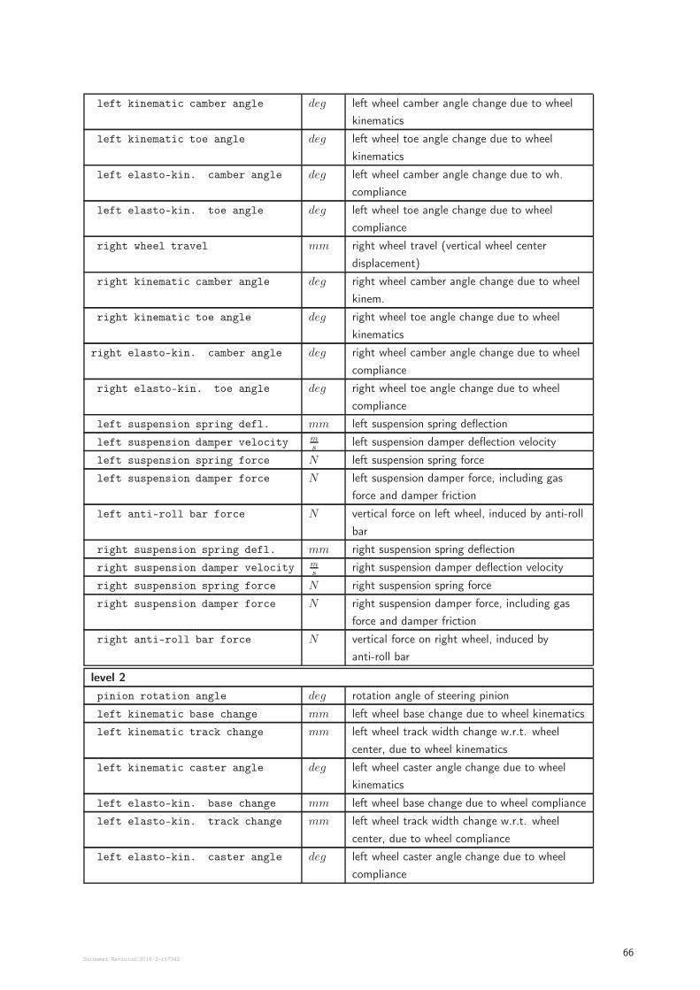
left kinematic camber angle deg left wheel camber angle change due to wheel
kinematics
left kinematic toe angle deg left wheel toe angle change due to wheel
kinematics
left elasto-kin. camber angle deg left wheel camber angle change due to wh.
compliance
left elasto-kin. toe angle deg left wheel toe angle change due to wheel
compliance
right wheel travel mm right wheel travel (vertical wheel center
displacement)
right kinematic camber angle deg right wheel camber angle change due to wheel
kinem.
right kinematic toe angle deg right wheel toe angle change due to wheel
kinematics
right elasto-kin. camber angle deg right wheel camber angle change due to wheel
compliance
right elasto-kin. toe angle deg right wheel toe angle change due to wheel
compliance
left suspension spring defl. mm left suspension spring deflection
left suspension damper velocity ms
left suspension damper deflection velocity
left suspension spring force N left suspension spring force
left suspension damper force N left suspension damper force, including gas
force and damper friction
left anti-roll bar force N vertical force on left wheel, induced by anti-roll
bar
right suspension spring defl. mm right suspension spring deflection
right suspension damper velocity ms
right suspension damper deflection velocity
right suspension spring force N right suspension spring force
right suspension damper force N right suspension damper force, including gas
force and damper friction
right anti-roll bar force N vertical force on right wheel, induced by
anti-roll bar
level 2
pinion rotation angle deg rotation angle of steering pinion
left kinematic base change mm left wheel base change due to wheel kinematics
left kinematic track change mm left wheel track width change w.r.t. wheel
center, due to wheel kinematics
left kinematic caster angle deg left wheel caster angle change due to wheel
kinematics
left elasto-kin. base change mm left wheel base change due to wheel compliance
left elasto-kin. track change mm left wheel track width change w.r.t. wheel
center, due to wheel compliance
left elasto-kin. caster angle deg left wheel caster angle change due to wheel
compliance
Document Revision:2018-2-r1734266
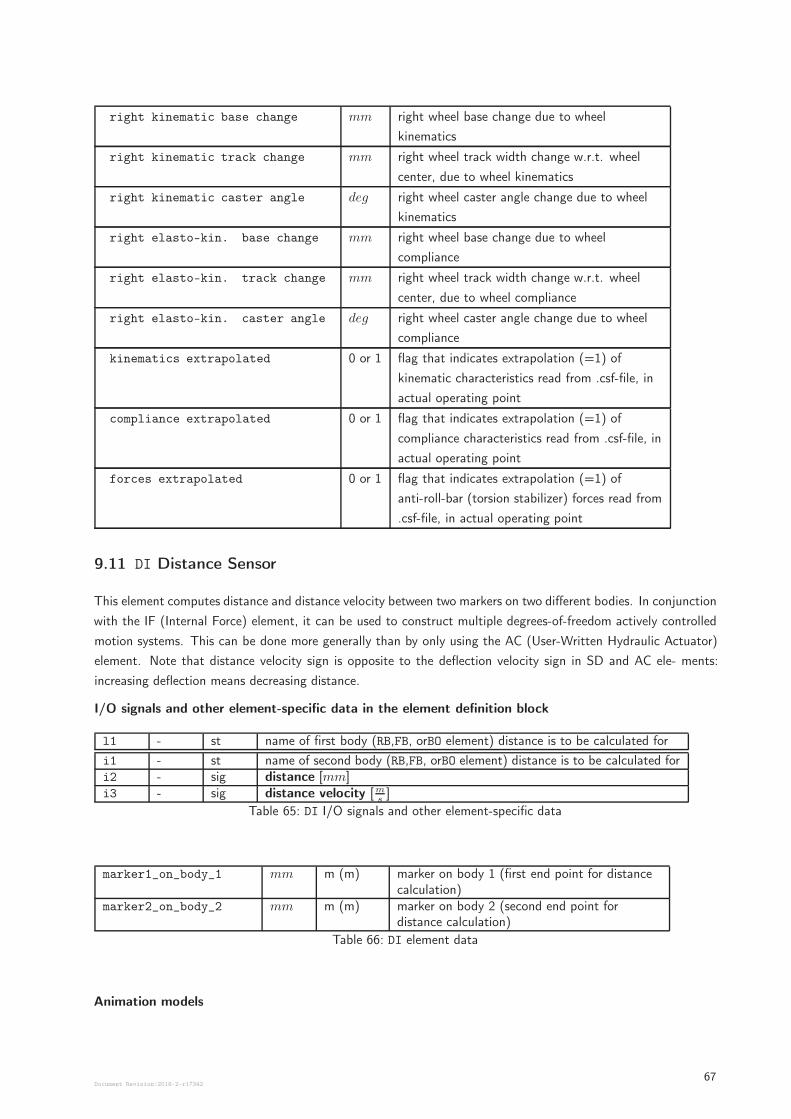
right kinematic base change mm right wheel base change due to wheel
kinematics
right kinematic track change mm right wheel track width change w.r.t. wheel
center, due to wheel kinematics
right kinematic caster angle deg right wheel caster angle change due to wheel
kinematics
right elasto-kin. base change mm right wheel base change due to wheel
compliance
right elasto-kin. track change mm right wheel track width change w.r.t. wheel
center, due to wheel compliance
right elasto-kin. caster angle deg right wheel caster angle change due to wheel
compliance
kinematics extrapolated 0 or 1 flag that indicates extrapolation (=1) of
kinematic characteristics read from .csf-file, in
actual operating point
compliance extrapolated 0 or 1 flag that indicates extrapolation (=1) of
compliance characteristics read from .csf-file, in
actual operating point
forces extrapolated 0 or 1 flag that indicates extrapolation (=1) of
anti-roll-bar (torsion stabilizer) forces read from
.csf-file, in actual operating point
9.11 DI Distance Sensor
This element computes distance and distance velocity between two markers on two different bodies. In conjunction
with the IF (Internal Force) element, it can be used to construct multiple degrees-of-freedom actively controlled
motion systems. This can be done more generally than by only using the AC (User-Written Hydraulic Actuator)
element. Note that distance velocity sign is opposite to the deflection velocity sign in SD and AC ele- ments:
increasing deflection means decreasing distance.
I/O signals and other element-specific data in the element definition block
l1 - st name of first body (RB,FB, orBO element) distance is to be calculated for
i1 - st name of second body (RB,FB, orBO element) distance is to be calculated fori2 - sig distance [mm]i3 - sig distance velocity [m
s]
Table 65: DI I/O signals and other element-specific data
marker1_on_body_1 mm m (m) marker on body 1 (first end point for distancecalculation)
marker2_on_body_2 mm m (m) marker on body 2 (second end point fordistance calculation)
Table 66: DI element data
Animation models
Document Revision:2018-2-r1734267
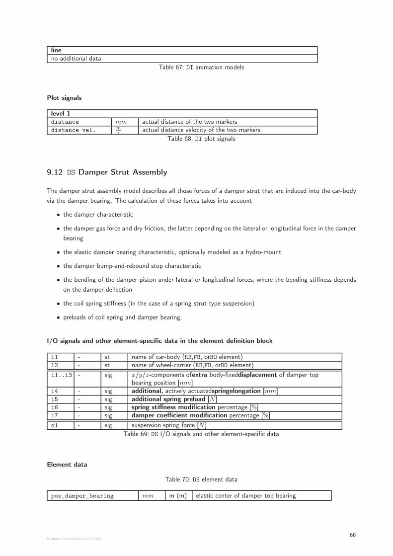
lineno additional data
Table 67: DI animation models
Plot signals
level 1distance mm actual distance of the two markersdistance vel. m
sactual distance velocity of the two markers
Table 68: DI plot signals
9.12 DS Damper Strut Assembly
The damper strut assembly model describes all those forces of a damper strut that are induced into the car-body
via the damper bearing. The calculation of these forces takes into account
• the damper characteristic
• the damper gas force and dry friction, the latter depending on the lateral or longitudinal force in the damper
bearing
• the elastic damper bearing characteristic, optionally modeled as a hydro-mount
• the damper bump-and-rebound stop characteristic
• the bending of the damper piston under lateral or longitudinal forces, where the bending stiffness depends
on the damper deflection
• the coil spring stiffness (in the case of a spring strut type suspension)
• preloads of coil spring and damper bearing.
I/O signals and other element-specific data in the element definition block
l1 - st name of car-body (RB,FB, orBO element)l2 - st name of wheel-carrier (RB,FB, orBO element)
i1..i3 - sig x/y/z-components ofextra body-fixeddisplacement of damper topbearing position [mm]
i4 - sig additional, actively actuatedspringelongation [mm]i5 - sig additional spring preload [N ]i6 - sig spring stiffness modification percentage [%]i7 - sig damper coefficient modification percentage [%]
o1 - sig suspension spring force [N ]
Table 69: DS I/O signals and other element-specific data
Element data
Table 70: DS element data
pos_damper_bearing mm m (m) elastic center of damper top bearing
Document Revision:2018-2-r1734268
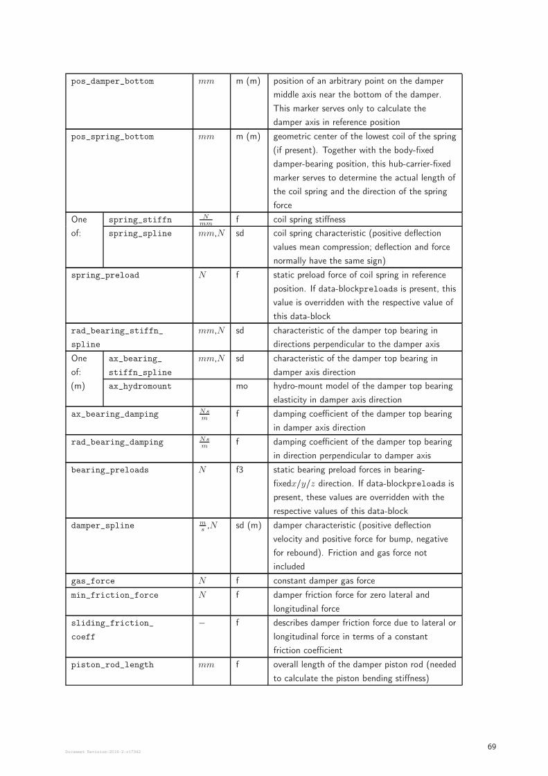
pos_damper_bottom mm m (m) position of an arbitrary point on the damper
middle axis near the bottom of the damper.
This marker serves only to calculate the
damper axis in reference position
pos_spring_bottom mm m (m) geometric center of the lowest coil of the spring
(if present). Together with the body-fixed
damper-bearing position, this hub-carrier-fixed
marker serves to determine the actual length of
the coil spring and the direction of the spring
force
One
of:
spring_stiffn Nmm
f coil spring stiffness
spring_spline mm,N sd coil spring characteristic (positive deflection
values mean compression; deflection and force
normally have the same sign)
spring_preload N f static preload force of coil spring in reference
position. If data-blockpreloads is present, this
value is overridden with the respective value of
this data-block
rad_bearing_stiffn_
spline
mm,N sd characteristic of the damper top bearing in
directions perpendicular to the damper axis
One
of:
(m)
ax_bearing_
stiffn_spline
mm,N sd characteristic of the damper top bearing in
damper axis direction
ax_hydromount mo hydro-mount model of the damper top bearing
elasticity in damper axis direction
ax_bearing_damping Nsm
f damping coefficient of the damper top bearing
in damper axis direction
rad_bearing_damping Nsm
f damping coefficient of the damper top bearing
in direction perpendicular to damper axis
bearing_preloads N f3 static bearing preload forces in bearing-
fixedx/y/z direction. If data-blockpreloads is
present, these values are overridden with the
respective values of this data-block
damper_spline ms,N sd (m) damper characteristic (positive deflection
velocity and positive force for bump, negative
for rebound). Friction and gas force not
included
gas_force N f constant damper gas force
min_friction_force N f damper friction force for zero lateral and
longitudinal force
sliding_friction_
coeff
− f describes damper friction force due to lateral or
longitudinal force in terms of a constant
friction coefficient
piston_rod_length mm f overall length of the damper piston rod (needed
to calculate the piston bending stiffness)
Document Revision:2018-2-r1734269
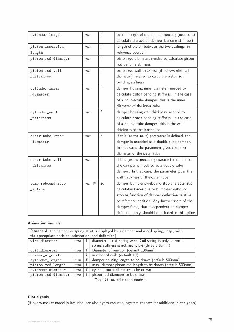
cylinder_length mm f overall length of the damper housing (needed to
calculate the overall damper bending stiffness)
piston_immersion_
length
mm f length of piston between the two sealings, in
reference position
piston_rod_diameter mm f piston rod diameter, needed to calculate piston
rod bending stiffness
piston_rod_wall
_thickness
mm f piston rod wall thickness (if hollow; else half
diameter), needed to calculate piston rod
bending stiffness
cylinder_inner
_diameter
mm f damper housing inner diameter, needed to
calculate piston bending stiffness. In the case
of a double-tube damper, this is the inner
diameter of the inner tube
cylinder_wall
_thickness
mm f damper housing wall thickness, needed to
calculate piston bending stiffness. In the case
of a double-tube damper, this is the wall
thickness of the inner tube
outer_tube_inner
_diameter
mm f if this (or the next) parameter is defined, the
damper is modeled as a double-tube damper.
In that case, the parameter gives the inner
diameter of the outer tube
outer_tube_wall
_thickness
mm f if this (or the preceding) parameter is defined,
the damper is modeled as a double-tube
damper. In that case, the parameter gives the
wall thickness of the outer tube
bump_rebound_stop
_spline
mm,N sd damper bump-and-rebound stop characteristic;
calculates forces due to bump-and-rebound
stop as function of damper deflection relative
to reference position. Any further share of the
damper force, that is dependent on damper
deflection only, should be included in this spline
Animation models
(standard: the damper or spring strut is displayed by a damper and a coil spring, resp., withthe appropriate position, orientation, and deflection)wire_diameter mm f diameter of coil spring wire. Coil spring is only shown if
spring stiffness is not negligible (default 10mm)coil_diameter mm f Diameter of one coil (default 100mm)number_of_coils − i number of coils (default 10)cylinder_length mm f damper housing length to be drawn (default 500mm)piston_rod length mm f max. damper piston rod length to be drawn (default 500mm)cylinder_diameter mm f cylinder outer diameter to be drawnpiston_rod_diameter mm f piston rod diameter to be drawn
Table 71: DS animation models
Plot signals
(if hydro-mount model is included, see also hydro-mount subsystem chapter for additional plot signals)
Document Revision:2018-2-r1734270
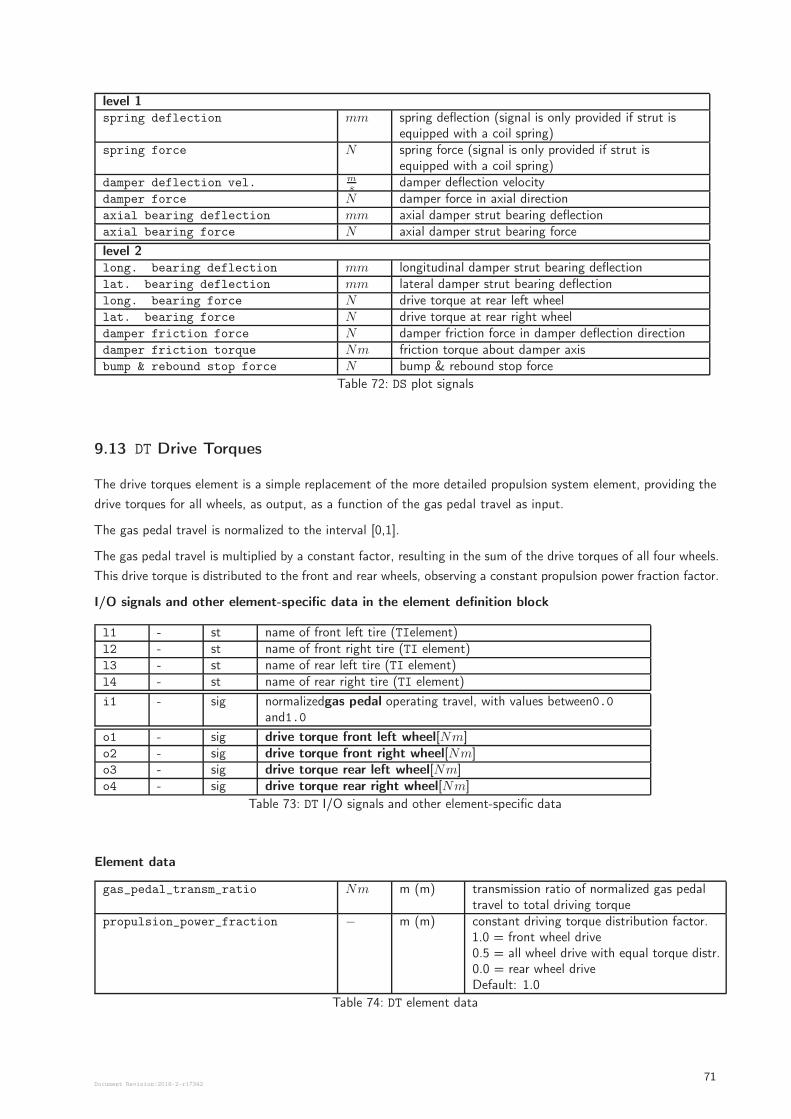
level 1spring deflection mm spring deflection (signal is only provided if strut is
equipped with a coil spring)spring force N spring force (signal is only provided if strut is
equipped with a coil spring)damper deflection vel. m
sdamper deflection velocity
damper force N damper force in axial directionaxial bearing deflection mm axial damper strut bearing deflectionaxial bearing force N axial damper strut bearing force
level 2long. bearing deflection mm longitudinal damper strut bearing deflectionlat. bearing deflection mm lateral damper strut bearing deflectionlong. bearing force N drive torque at rear left wheellat. bearing force N drive torque at rear right wheeldamper friction force N damper friction force in damper deflection directiondamper friction torque Nm friction torque about damper axisbump & rebound stop force N bump & rebound stop force
Table 72: DS plot signals
9.13 DT Drive Torques
The drive torques element is a simple replacement of the more detailed propulsion system element, providing the
drive torques for all wheels, as output, as a function of the gas pedal travel as input.
The gas pedal travel is normalized to the interval [0,1].
The gas pedal travel is multiplied by a constant factor, resulting in the sum of the drive torques of all four wheels.
This drive torque is distributed to the front and rear wheels, observing a constant propulsion power fraction factor.
I/O signals and other element-specific data in the element definition block
l1 - st name of front left tire (TIelement)l2 - st name of front right tire (TI element)l3 - st name of rear left tire (TI element)l4 - st name of rear right tire (TI element)
i1 - sig normalizedgas pedal operating travel, with values between0.0and1.0
o1 - sig drive torque front left wheel[Nm]o2 - sig drive torque front right wheel[Nm]o3 - sig drive torque rear left wheel[Nm]o4 - sig drive torque rear right wheel[Nm]
Table 73: DT I/O signals and other element-specific data
Element data
gas_pedal_transm_ratio Nm m (m) transmission ratio of normalized gas pedaltravel to total driving torque
propulsion_power_fraction − m (m) constant driving torque distribution factor.1.0 = front wheel drive0.5 = all wheel drive with equal torque distr.0.0 = rear wheel driveDefault: 1.0
Table 74: DT element data
Document Revision:2018-2-r1734271
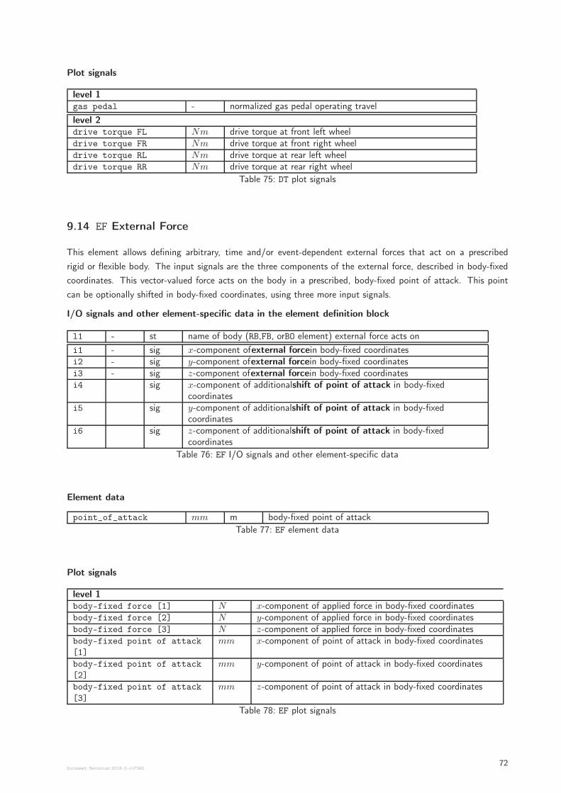
Plot signals
level 1gas pedal - normalized gas pedal operating travel
level 2drive torque FL Nm drive torque at front left wheeldrive torque FR Nm drive torque at front right wheeldrive torque RL Nm drive torque at rear left wheeldrive torque RR Nm drive torque at rear right wheel
Table 75: DT plot signals
9.14 EF External Force
This element allows defining arbitrary, time and/or event-dependent external forces that act on a prescribed
rigid or flexible body. The input signals are the three components of the external force, described in body-fixed
coordinates. This vector-valued force acts on the body in a prescribed, body-fixed point of attack. This point
can be optionally shifted in body-fixed coordinates, using three more input signals.
I/O signals and other element-specific data in the element definition block
l1 - st name of body (RB,FB, orBO element) external force acts on
i1 - sig x-component ofexternal forcein body-fixed coordinatesi2 - sig y-component ofexternal forcein body-fixed coordinatesi3 - sig z-component ofexternal forcein body-fixed coordinatesi4 sig x-component of additionalshift of point of attack in body-fixed
coordinatesi5 sig y-component of additionalshift of point of attack in body-fixed
coordinatesi6 sig z-component of additionalshift of point of attack in body-fixed
coordinates
Table 76: EF I/O signals and other element-specific data
Element data
point_of_attack mm m body-fixed point of attack
Table 77: EF element data
Plot signals
level 1body-fixed force [1] N x-component of applied force in body-fixed coordinatesbody-fixed force [2] N y-component of applied force in body-fixed coordinatesbody-fixed force [3] N z-component of applied force in body-fixed coordinatesbody-fixed point of attack
[1]
mm x-component of point of attack in body-fixed coordinates
body-fixed point of attack
[2]
mm y-component of point of attack in body-fixed coordinates
body-fixed point of attack
[3]
mm z-component of point of attack in body-fixed coordinates
Table 78: EF plot signals
Document Revision:2018-2-r1734272
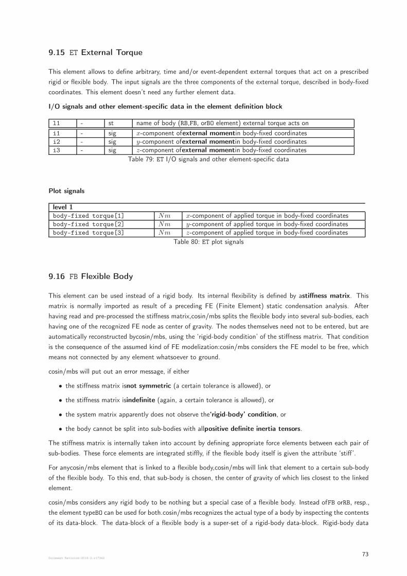
9.15 ET External Torque
This element allows to define arbitrary, time and/or event-dependent external torques that act on a prescribed
rigid or flexible body. The input signals are the three components of the external torque, described in body-fixed
coordinates. This element doesn’t need any further element data.
I/O signals and other element-specific data in the element definition block
l1 - st name of body (RB,FB, orBO element) external torque acts on
i1 - sig x-component ofexternal momentin body-fixed coordinatesi2 - sig y-component ofexternal momentin body-fixed coordinatesi3 - sig z-component ofexternal momentin body-fixed coordinates
Table 79: ET I/O signals and other element-specific data
Plot signals
level 1body-fixed torque[1] Nm x-component of applied torque in body-fixed coordinatesbody-fixed torque[2] Nm y-component of applied torque in body-fixed coordinatesbody-fixed torque[3] Nm z-component of applied torque in body-fixed coordinates
Table 80: ET plot signals
9.16 FB Flexible Body
This element can be used instead of a rigid body. Its internal flexibility is defined by astiffness matrix. This
matrix is normally imported as result of a preceding FE (Finite Element) static condensation analysis. After
having read and pre-processed the stiffness matrix,cosin/mbs splits the flexible body into several sub-bodies, each
having one of the recognized FE node as center of gravity. The nodes themselves need not to be entered, but are
automatically reconstructed bycosin/mbs, using the ‘rigid-body condition’ of the stiffness matrix. That condition
is the consequence of the assumed kind of FE modelization:cosin/mbs considers the FE model to be free, which
means not connected by any element whatsoever to ground.
cosin/mbs will put out an error message, if either
• the stiffness matrix isnot symmetric (a certain tolerance is allowed), or
• the stiffness matrix isindefinite (again, a certain tolerance is allowed), or
• the system matrix apparently does not observe the‘rigid-body’ condition, or
• the body cannot be split into sub-bodies with allpositive definite inertia tensors.
The stiffness matrix is internally taken into account by defining appropriate force elements between each pair of
sub-bodies. These force elements are integrated stiffly, if the flexible body itself is given the attribute ‘stiff’.
For anycosin/mbs element that is linked to a flexible body,cosin/mbs will link that element to a certain sub-body
of the flexible body. To this end, that sub-body is chosen, the center of gravity of which lies closest to the linked
element.
cosin/mbs considers any rigid body to be nothing but a special case of a flexible body. Instead ofFB orRB, resp.,
the element typeBO can be used for both.cosin/mbs recognizes the actual type of a body by inspecting the contents
of its data-block. The data-block of a flexible body is a super-set of a rigid-body data-block. Rigid-body data
Document Revision:2018-2-r1734273
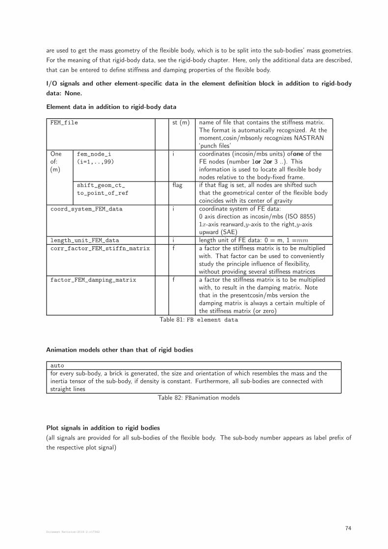
are used to get the mass geometry of the flexible body, which is to be split into the sub-bodies’ mass geometries.
For the meaning of that rigid-body data, see the rigid-body chapter. Here, only the additional data are described,
that can be entered to define stiffness and damping properties of the flexible body.
I/O signals and other element-specific data in the element definition block in addition to rigid-body
data: None.
Element data in addition to rigid-body data
FEM_file st (m) name of file that contains the stiffness matrix.The format is automatically recognized. At themoment,cosin/mbsonly recognizes NASTRAN‘punch files’
Oneof:(m)
fem_node_i
(i=1,..,99)
i coordinates (incosin/mbs units) ofone of theFE nodes (number 1or 2or 3 ..). Thisinformation is used to locate all flexible bodynodes relative to the body-fixed frame.
shift_geom_ct_
to_point_of_ref
flag if that flag is set, all nodes are shifted suchthat the geometrical center of the flexible bodycoincides with its center of gravity
coord_system_FEM_data i coordinate system of FE data:0 axis direction as incosin/mbs (ISO 8855)1x-axis rearward,y-axis to the right,y-axisupward (SAE)
length_unit_FEM_data i length unit of FE data: 0 = m, 1 =mmcorr_factor_FEM_stiffn_matrix f a factor the stiffness matrix is to be multiplied
with. That factor can be used to convenientlystudy the principle influence of flexibility,without providing several stiffness matrices
factor_FEM_damping_matrix f a factor the stiffness matrix is to be multipliedwith, to result in the damping matrix. Notethat in the presentcosin/mbs version thedamping matrix is always a certain multiple ofthe stiffness matrix (or zero)
Table 81: FB element data
Animation models other than that of rigid bodies
auto
for every sub-body, a brick is generated, the size and orientation of which resembles the mass and theinertia tensor of the sub-body, if density is constant. Furthermore, all sub-bodies are connected withstraight lines
Table 82: FBanimation models
Plot signals in addition to rigid bodies
(all signals are provided for all sub-bodies of the flexible body. The sub-body number appears as label prefix of
the respective plot signal)
Document Revision:2018-2-r1734274
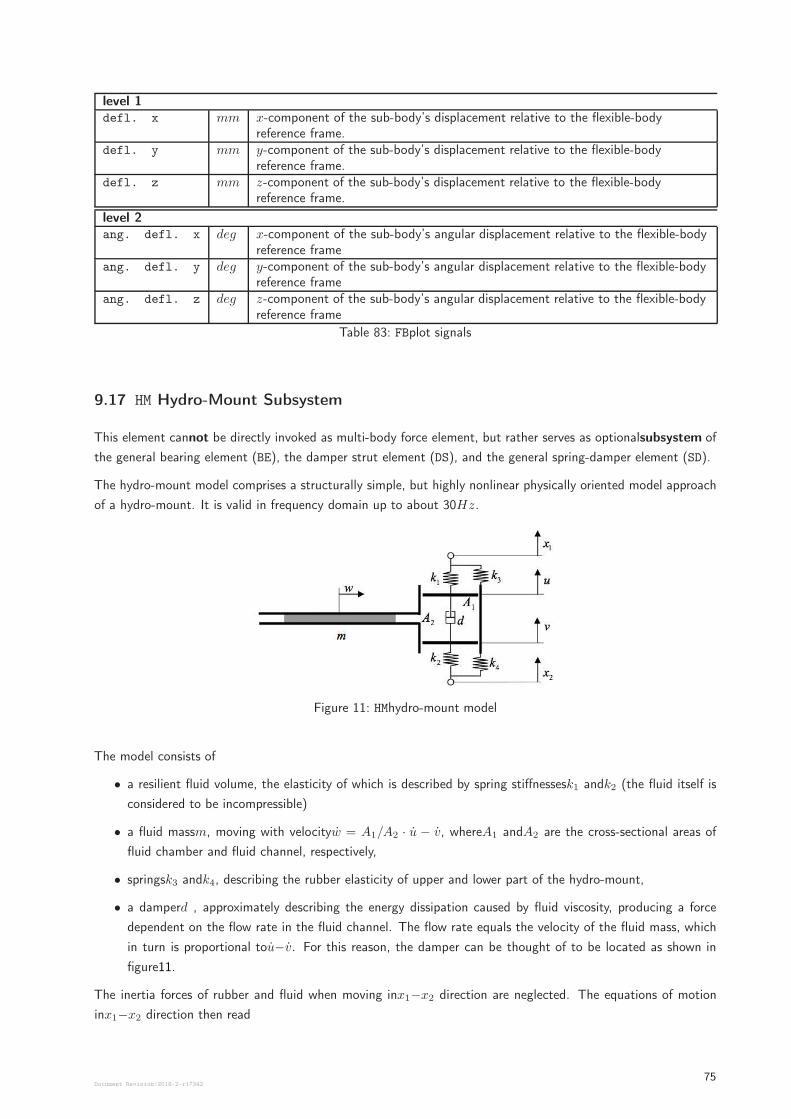
level 1defl. x mm x-component of the sub-body’s displacement relative to the flexible-body
reference frame.defl. y mm y-component of the sub-body’s displacement relative to the flexible-body
reference frame.defl. z mm z-component of the sub-body’s displacement relative to the flexible-body
reference frame.
level 2ang. defl. x deg x-component of the sub-body’s angular displacement relative to the flexible-body
reference frameang. defl. y deg y-component of the sub-body’s angular displacement relative to the flexible-body
reference frameang. defl. z deg z-component of the sub-body’s angular displacement relative to the flexible-body
reference frame
Table 83: FBplot signals
9.17 HM Hydro-Mount Subsystem
This element cannot be directly invoked as multi-body force element, but rather serves as optionalsubsystem of
the general bearing element (BE), the damper strut element (DS), and the general spring-damper element (SD).
The hydro-mount model comprises a structurally simple, but highly nonlinear physically oriented model approach
of a hydro-mount. It is valid in frequency domain up to about 30Hz.
Figure 11: HMhydro-mount model
The model consists of
• a resilient fluid volume, the elasticity of which is described by spring stiffnessesk1 andk2 (the fluid itself is
considered to be incompressible)
• a fluid massm, moving with velocityw = A1/A2 · u − v, whereA1 andA2 are the cross-sectional areas of
fluid chamber and fluid channel, respectively,
• springsk3 andk4, describing the rubber elasticity of upper and lower part of the hydro-mount,
• a damperd , approximately describing the energy dissipation caused by fluid viscosity, producing a force
dependent on the flow rate in the fluid channel. The flow rate equals the velocity of the fluid mass, which
in turn is proportional tou−v. For this reason, the damper can be thought of to be located as shown in
figure11.
The inertia forces of rubber and fluid when moving inx1−x2 direction are neglected. The equations of motion
inx1−x2 direction then read
Document Revision:2018-2-r1734275
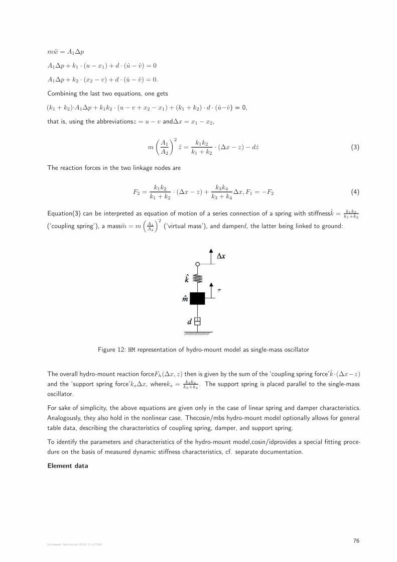
mw = A1∆p
A1∆p+ k1 · (u− x1) + d · (u− v) = 0
A1∆p+ k2 · (x2 − v) + d · (u− v) = 0.
Combining the last two equations, one gets
(k1 + k2)·A1∆p+ k1k2 · (u− v + x2 − x1) + (k1 + k2) · d · (u−v) = 0,
that is, using the abbreviationsz = u− v and∆x = x1 − x2,
m
(
A1
A2
)2
z =k1k2
k1 + k2· (∆x− z)− dz (3)
The reaction forces in the two linkage nodes are
F2 =k1k2
k1 + k2· (∆x− z) +
k3k4k3 + k4
∆x, F1 = −F2 (4)
Equation(3) can be interpreted as equation of motion of a series connection of a spring with stiffnessk = k1k2
k1+k2
(‘coupling spring’), a massm = m(
A1
A2
)2
(‘virtual mass’), and damperd, the latter being linked to ground:
Figure 12: HM representation of hydro-mount model as single-mass oscillator
The overall hydro-mount reaction forceFh(∆x, z) then is given by the sum of the ‘coupling spring force’k ·(∆x−z)
and the ‘support spring force’ks∆x, whereks = k3k4
k3+k4. The support spring is placed parallel to the single-mass
oscillator.
For sake of simplicity, the above equations are given only in the case of linear spring and damper characteristics.
Analogously, they also hold in the nonlinear case. Thecosin/mbs hydro-mount model optionally allows for general
table data, describing the characteristics of coupling spring, damper, and support spring.
To identify the parameters and characteristics of the hydro-mount model,cosin/idprovides a special fitting proce-
dure on the basis of measured dynamic stiffness characteristics, cf. separate documentation.
Element data
Document Revision:2018-2-r1734276
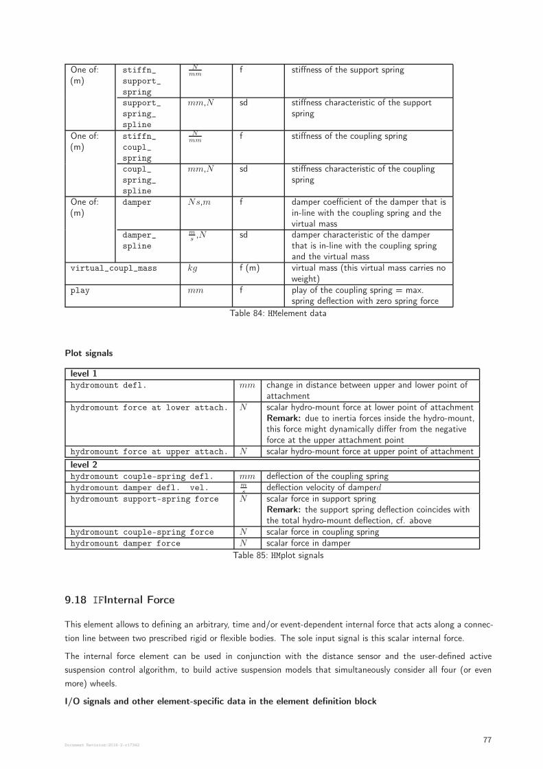
One of:(m)
stiffn_
support_
spring
Nmm
f stiffness of the support spring
support_
spring_
spline
mm,N sd stiffness characteristic of the supportspring
One of:(m)
stiffn_
coupl_
spring
Nmm
f stiffness of the coupling spring
coupl_
spring_
spline
mm,N sd stiffness characteristic of the couplingspring
One of:(m)
damper Ns,m f damper coefficient of the damper that isin-line with the coupling spring and thevirtual mass
damper_
spline
ms,N sd damper characteristic of the damper
that is in-line with the coupling springand the virtual mass
virtual_coupl_mass kg f (m) virtual mass (this virtual mass carries noweight)
play mm f play of the coupling spring = max.spring deflection with zero spring force
Table 84: HMelement data
Plot signals
level 1hydromount defl. mm change in distance between upper and lower point of
attachmenthydromount force at lower attach. N scalar hydro-mount force at lower point of attachment
Remark: due to inertia forces inside the hydro-mount,this force might dynamically differ from the negativeforce at the upper attachment point
hydromount force at upper attach. N scalar hydro-mount force at upper point of attachment
level 2hydromount couple-spring defl. mm deflection of the coupling springhydromount damper defl. vel. m
sdeflection velocity of damperd
hydromount support-spring force N scalar force in support springRemark: the support spring deflection coincides withthe total hydro-mount deflection, cf. above
hydromount couple-spring force N scalar force in coupling springhydromount damper force N scalar force in damper
Table 85: HMplot signals
9.18 IFInternal Force
This element allows to defining an arbitrary, time and/or event-dependent internal force that acts along a connec-
tion line between two prescribed rigid or flexible bodies. The sole input signal is this scalar internal force.
The internal force element can be used in conjunction with the distance sensor and the user-defined active
suspension control algorithm, to build active suspension models that simultaneously consider all four (or even
more) wheels.
I/O signals and other element-specific data in the element definition block
Document Revision:2018-2-r1734277
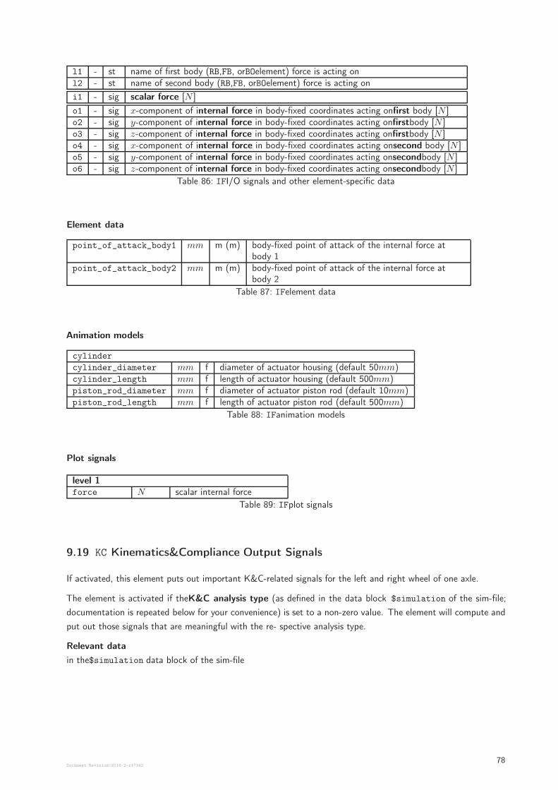
l1 - st name of first body (RB,FB, orBOelement) force is acting onl2 - st name of second body (RB,FB, orBOelement) force is acting on
i1 - sig scalar force [N ]
o1 - sig x-component of internal force in body-fixed coordinates acting onfirst body [N ]o2 - sig y-component of internal force in body-fixed coordinates acting onfirstbody [N ]o3 - sig z-component of internal force in body-fixed coordinates acting onfirstbody [N ]o4 - sig x-component of internal force in body-fixed coordinates acting onsecond body [N ]o5 - sig y-component of internal force in body-fixed coordinates acting onsecondbody [N ]o6 - sig z-component of internal force in body-fixed coordinates acting onsecondbody [N ]
Table 86: IFI/O signals and other element-specific data
Element data
point_of_attack_body1 mm m (m) body-fixed point of attack of the internal force atbody 1
point_of_attack_body2 mm m (m) body-fixed point of attack of the internal force atbody 2
Table 87: IFelement data
Animation models
cylinder
cylinder_diameter mm f diameter of actuator housing (default 50mm)cylinder_length mm f length of actuator housing (default 500mm)piston_rod_diameter mm f diameter of actuator piston rod (default 10mm)piston_rod_length mm f length of actuator piston rod (default 500mm)
Table 88: IFanimation models
Plot signals
level 1force N scalar internal force
Table 89: IFplot signals
9.19 KC Kinematics&Compliance Output Signals
If activated, this element puts out important K&C-related signals for the left and right wheel of one axle.
The element is activated if theK&C analysis type (as defined in the data block $simulation of the sim-file;
documentation is repeated below for your convenience) is set to a non-zero value. The element will compute and
put out those signals that are meaningful with the re- spective analysis type.
Relevant data
in the$simulation data block of the sim-file
Document Revision:2018-2-r1734278
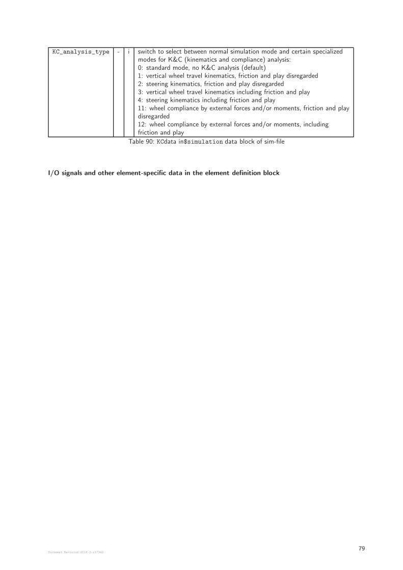
KC_analysis_type - i switch to select between normal simulation mode and certain specializedmodes for K&C (kinematics and compliance) analysis:0: standard mode, no K&C analysis (default)1: vertical wheel travel kinematics, friction and play disregarded2: steering kinematics, friction and play disregarded3: vertical wheel travel kinematics including friction and play4: steering kinematics including friction and play11: wheel compliance by external forces and/or moments, friction and playdisregarded12: wheel compliance by external forces and/or moments, includingfriction and play
Table 90: KCdata in$simulation data block of sim-file
I/O signals and other element-specific data in the element definition block
Document Revision:2018-2-r1734279
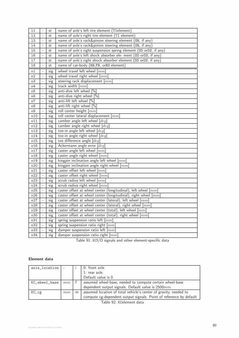
l1 - st name of axle’s left tire element (TIelement)l2 - st name of axle’s right tire element (TI element)l3 - st name of axle’s rack&pinion steering element (SR, if any)l4 - st name of axle’s rack&pinion steering element (SR, if any)l5 - st name of axle’s right suspension spring element (SD orDS, if any)l6 - st name of axle’s left shock absorber ele- ment (SD orDS, if any)l7 - st name of axle’s right shock absorber element (SD orDS, if any)l8 - st name of car-body (RB,FB, orBO element)
o1 - sig wheel travel left wheel [mm]o2 - sig wheel travel right wheel [mm]o3 - sig steering rack displacement [mm]o4 - sig track width [mm]o5 - sig anti-dive left wheel [%]o6 - sig anti-dive right wheel [%]o7 - sig anti-lift left wheel [%]o8 - sig anti-lift right wheel [%]o9 - sig roll center height [mm]o10 - sig roll center lateral displacement [mm]o11 - sig camber angle left wheel [deg]o12 - sig camber angle right wheel [deg]o13 - sig toe-in angle left wheel [deg]o14 - sig toe-in angle right wheel [deg]o15 - sig toe difference angle [deg]o16 - sig Ackermann angle error [deg]o17 - sig caster angle left wheel [mm]o18 - sig caster angle right wheel [mm]o19 - sig kingpin inclination angle left wheel [mm]o20 - sig kingpin inclination angle right wheel [mm]o21 - sig caster offset left wheel [mm]o22 - sig caster offset right wheel [mm]o23 - sig scrub radius left wheel [mm]o24 - sig scrub radius right wheel [mm]o25 - sig caster offset at wheel center (longitudinal), left wheel [mm]o26 - sig caster offset at wheel center (longitudinal), right wheel [mm]o27 - sig caster offset at wheel center (lateral), left wheel [mm]o28 - sig caster offset at wheel center (lateral), right wheel [mm]o29 - sig caster offset at wheel center (total), left wheel [mm]o30 - sig caster offset at wheel center (total), right wheel [mm]o31 - sig spring suspension ratio left [mm]o32 - sig spring suspension ratio right [mm]o33 - sig damper suspension ratio left [mm]o34 - sig damper suspension ratio right [mm]
Table 91: KCI/O signals and other element-specific data
Element data
axis_location - i 0: front axle1: rear axle.Default value is 0
KC_wheel_base mm f assumed wheel-base, needed to compute certain wheel-basedependent output signals. Default value is 2500mm
KC_cg mm m assumed location of total vehicle’s center of gravity, needed tocompute cg-dependent output signals. Point of reference by default
Table 92: KCelement data
Document Revision:2018-2-r1734280
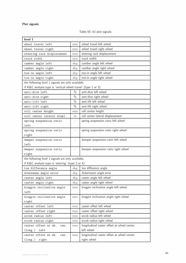
Plot signals
Table 93: KC plot signals
level 1
wheel travel left mm wheel travel left wheel
wheel travel right mm wheel travel right wheel
steering rack displacement mm steering rack displacement
track width mm track width
camber angle left deg camber angle left wheel
camber angle right deg camber angle right wheel
toe-in angle left deg toe-in angle left wheel
toe-in angle right deg toe-in angle right wheel
the following level 1 signals are only available,
if K&C analysis type is ‘vertical wheel travel’ (type 1 or 3)
anti-dive left % anti-dive left wheel
anti-dive right % anti-dive right wheel
anti-lift left % anti-lift left wheel
anti-lift right % anti-lift right wheel
roll center height mm roll center height
roll center lateral displ. m roll center lateral displacement
spring suspension ratio
left
- spring suspension ratio left wheel
spring suspension ratio
right
- spring suspension ratio right wheel
damper suspension ratio
left
- damper suspension ratio left wheel
damper suspension ratio
right
- damper suspension ratio right wheel
the following level 1 signals are only available,
if K&C analysis type is ‘steering’ (type 2 or 4)
toe difference angle deg toe difference angle
Ackermann angle error deg Ackermann angle error
caster angle left deg caster angle left wheel
caster angle right deg caster angle right wheel
kingpin inclination angle
left
mm kingpin inclination angle left wheel
kingpin inclination angle
right
mm kingpin inclination angle right wheel
caster offset left mm caster offset left wheel
caster offset right mm caster offset right wheel
scrub radius left mm scrub radius left wheel
scrub radius right mm scrub radius right wheel
caster offset at wh. cen.
(long.) left
mm longitudinal caster offset at wheel center,
left wheel
caster offset at wh. cen.
(long.) right
mm longitudinal caster offset at wheel center,
right wheel
Document Revision:2018-2-r1734281
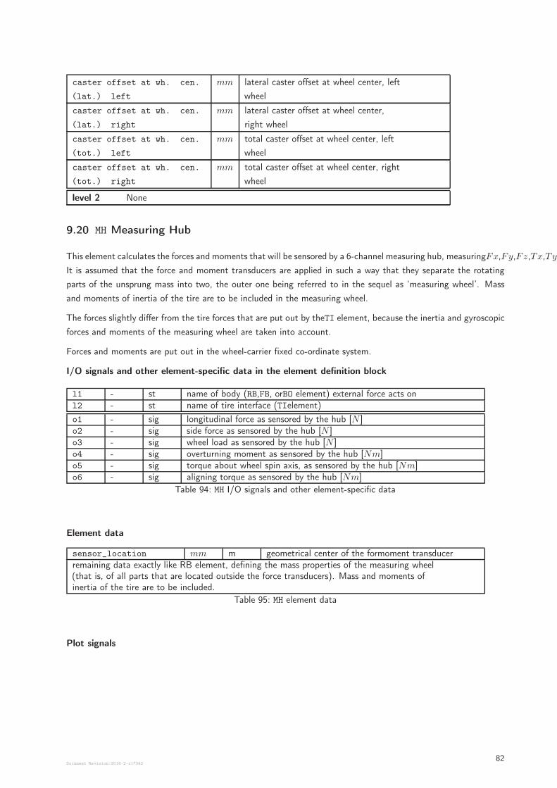
caster offset at wh. cen.
(lat.) left
mm lateral caster offset at wheel center, left
wheel
caster offset at wh. cen.
(lat.) right
mm lateral caster offset at wheel center,
right wheel
caster offset at wh. cen.
(tot.) left
mm total caster offset at wheel center, left
wheel
caster offset at wh. cen.
(tot.) right
mm total caster offset at wheel center, right
wheel
level 2 None
9.20 MH Measuring Hub
This element calculates the forces and moments that will be sensored by a 6-channel measuring hub, measuringFx,Fy,Fz,Tx,Ty,Tz.
It is assumed that the force and moment transducers are applied in such a way that they separate the rotating
parts of the unsprung mass into two, the outer one being referred to in the sequel as ‘measuring wheel’. Mass
and moments of inertia of the tire are to be included in the measuring wheel.
The forces slightly differ from the tire forces that are put out by theTI element, because the inertia and gyroscopic
forces and moments of the measuring wheel are taken into account.
Forces and moments are put out in the wheel-carrier fixed co-ordinate system.
I/O signals and other element-specific data in the element definition block
l1 - st name of body (RB,FB, orBO element) external force acts onl2 - st name of tire interface (TIelement)
o1 - sig longitudinal force as sensored by the hub [N ]o2 - sig side force as sensored by the hub [N ]o3 - sig wheel load as sensored by the hub [N ]o4 - sig overturning moment as sensored by the hub [Nm]o5 - sig torque about wheel spin axis, as sensored by the hub [Nm]o6 - sig aligning torque as sensored by the hub [Nm]
Table 94: MH I/O signals and other element-specific data
Element data
sensor_location mm m geometrical center of the formoment transducerremaining data exactly like RB element, defining the mass properties of the measuring wheel(that is, of all parts that are located outside the force transducers). Mass and moments ofinertia of the tire are to be included.
Table 95: MH element data
Plot signals
Document Revision:2018-2-r1734282
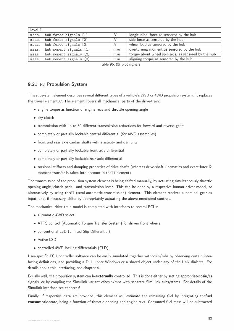
level 1meas. hub force signals [1] N longitudinal force as sensored by the hubmeas. hub force signals [2] N side force as sensored by the hubmeas. hub force signals [3] N wheel load as sensored by the hubmeas. hub moment signals [1] mm overturning moment as sensored by the hubmeas. hub moment signals [2] mm torque about wheel spin axis, as sensored by the hubmeas. hub moment signals [3] mm aligning torque as sensored by the hub
Table 96: MH plot signals
9.21 PS Propulsion System
This subsystem element describes several different types of a vehicle’s 2WD or 4WD propulsion system. It replaces
the trivial elementDT. The element covers all mechanical parts of the drive-train:
• engine torque as function of engine revs and throttle opening angle
• dry clutch
• transmission with up to 30 different transmission reductions for forward and reverse gears
• completely or partially lockable central differential (for 4WD assemblies)
• front and rear axle cardan shafts with elasticity and damping
• completely or partially lockable front axle differential
• completely or partially lockable rear axle differential
• torsional stiffness and damping properties of drive shafts (whereas drive-shaft kinematics and exact force &
moment transfer is taken into account in theTI element).
The transmission of the propulsion system element is being shifted manually, by actuating simultaneously throttle
opening angle, clutch pedal, and transmission lever. This can be done by a respective human driver model, or
alternatively by using theST (semi-automatic transmission) element. This element receives a nominal gear as
input, and, if necessary, shifts by appropriately actuating the above-mentioned controls.
The mechanical drive-train model is completed with interfaces to several ECUs:
• automatic 4WD select
• ATTS control (Automatic Torque Transfer System) for driven front wheels
• conventional LSD (Limited Slip Differential)
• Active LSD
• controlled 4WD locking differentials (CLD).
User-specific ECU controller software can be easily simulated together withcosin/mbs by observing certain inter-
facing definitions, and providing a DLL under Windows or a shared object under any of the Unix dialects. For
details about this interfacing, see chapter 4.
Equally well, the propulsion system can beexternally controlled. This is done either by setting appropriatecosin/ss
signals, or by coupling the Simulink variant ofcosin/mbs with separate Simulink subsystems. For details of the
Simulink interface see chapter 6.
Finally, if respective data are provided, this element will estimate the remaining fuel by integrating thefuel
consumptionrate, being a function of throttle opening and engine revs. Consumed fuel mass will be subtracted
Document Revision:2018-2-r1734283
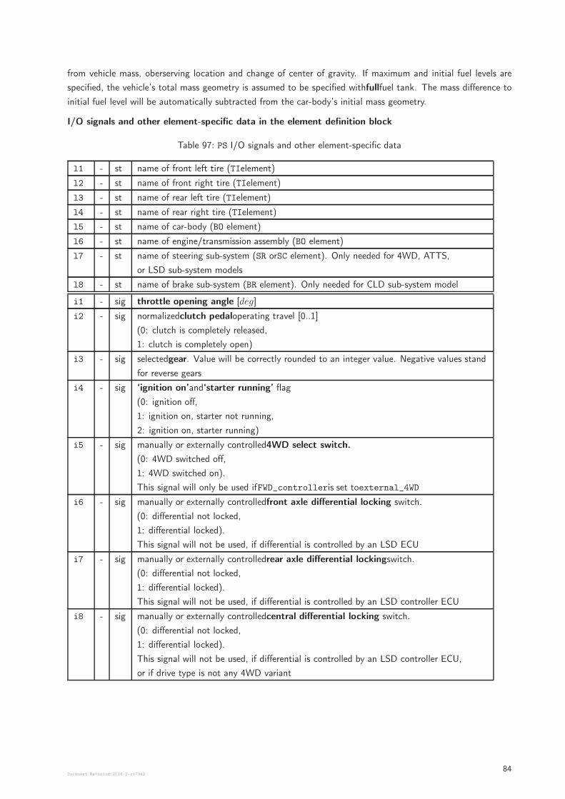
from vehicle mass, oberserving location and change of center of gravity. If maximum and initial fuel levels are
specified, the vehicle’s total mass geometry is assumed to be specified withfullfuel tank. The mass difference to
initial fuel level will be automatically subtracted from the car-body’s initial mass geometry.
I/O signals and other element-specific data in the element definition block
Table 97: PS I/O signals and other element-specific data
l1 - st name of front left tire (TIelement)
l2 - st name of front right tire (TIelement)
l3 - st name of rear left tire (TIelement)
l4 - st name of rear right tire (TIelement)
l5 - st name of car-body (BO element)
l6 - st name of engine/transmission assembly (BO element)
l7 - st name of steering sub-system (SR orSC element). Only needed for 4WD, ATTS,
or LSD sub-system models
l8 - st name of brake sub-system (BR element). Only needed for CLD sub-system model
i1 - sig throttle opening angle [deg]
i2 - sig normalizedclutch pedaloperating travel [0..1]
(0: clutch is completely released,
1: clutch is completely open)
i3 - sig selectedgear. Value will be correctly rounded to an integer value. Negative values stand
for reverse gears
i4 - sig ‘ignition on’and‘starter running’ flag
(0: ignition off,
1: ignition on, starter not running,
2: ignition on, starter running)
i5 - sig manually or externally controlled4WD select switch.
(0: 4WD switched off,
1: 4WD switched on).
This signal will only be used ifFWD_controlleris set toexternal_4WD
i6 - sig manually or externally controlledfront axle differential locking switch.
(0: differential not locked,
1: differential locked).
This signal will not be used, if differential is controlled by an LSD ECU
i7 - sig manually or externally controlledrear axle differential lockingswitch.
(0: differential not locked,
1: differential locked).
This signal will not be used, if differential is controlled by an LSD controller ECU
i8 - sig manually or externally controlledcentral differential locking switch.
(0: differential not locked,
1: differential locked).
This signal will not be used, if differential is controlled by an LSD controller ECU,
or if drive type is not any 4WD variant
Document Revision:2018-2-r1734284
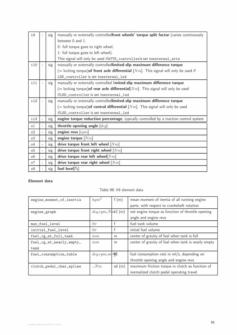
i9 - sig manually or externally controlledfront wheels’ torque split factor (varies continuously
between 0 and 1.
0: full torque goes to right wheel,
1: full torque goes to left wheel).
This signal will only be used ifATTS_controlleris set toexternal_atts
i10 - sig manually or externally controlledlimited-slip maximum difference torque
(= locking torque)of front axle differential [Nm]. This signal will only be used if
LSD_controller is set toexternal_lsd
i11 - sig manually or externally controlled limited-slip maximum difference torque
(= locking torque)of rear axle differential[Nm]. This signal will only be used
ifLSD_controller is set toexternal_lsd
i12 - sig manually or externally controlledlimited-slip maximum difference torque
(= locking torque)of central differential [Nm]. This signal will only be used
ifLSD_controller is set toexternal_lsd
i13 - sig engine torque reduction percentage, typically controlled by a traction control system
o1 - sig throttle opening angle [deg]
o2 - sig engine revs [rpm]
o3 - sig engine torque [Nm]
o4 - sig drive torque front left wheel [Nm]
o5 - sig drive torque front right wheel [Nm]
o6 - sig drive torque rear left wheel[Nm]
o7 - sig drive torque rear right wheel [Nm]
o8 - sig fuel level[%]
Element data
Table 98: PS element data
engine_moment_of_inertia kgm2 f (m) mean moment of inertia of all running engine
parts, with respect to crankshaft rotation
engine_graph deg,rpm,Nmt2 (m) net engine torque as function of throttle opening
angle and engine revs
max_fuel_level ltr f fuel tank volume
initial_fuel_level ltr f initial fuel volume
fuel_cg_at_full_tank mm m center of gravity of fuel when tank is full
fuel_cg_at_nearly_empty_
tank
mm m center of gravity of fuel when tank is nearly empty
fuel_consumption_table deg,rpm,m,mlst2 fuel consumption rate in ml/s, depending on
throttle opening angle and engine revs
clutch_pedal_char_spline -,Nm sd (m) maximum friction torque in clutch as function of
normalized clutch pedal operating travel
Document Revision:2018-2-r1734285
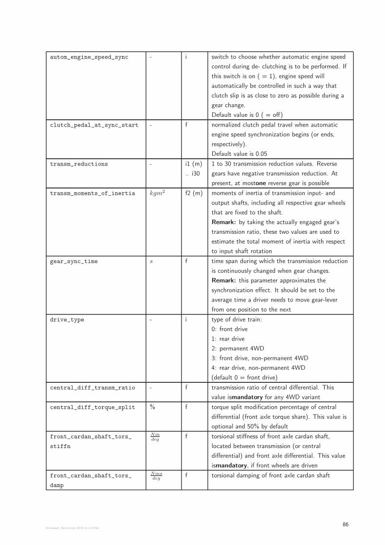
autom_engine_speed_sync - i switch to choose whether automatic engine speed
control during de- clutching is to be performed. If
this switch is on ( = 1), engine speed will
automatically be controlled in such a way that
clutch slip is as close to zero as possible during a
gear change.
Default value is 0 ( = off)
clutch_pedal_at_sync_start - f normalized clutch pedal travel when automatic
engine speed synchronization begins (or ends,
respectively).
Default value is 0.05
transm_reductions - i1 (m)
.. i30
1 to 30 transmission reduction values. Reverse
gears have negative transmission reduction. At
present, at mostone reverse gear is possible
transm_moments_of_inertia kgm2 f2 (m) moments of inertia of transmission input- and
output shafts, including all respective gear wheels
that are fixed to the shaft.
Remark: by taking the actually engaged gear’s
transmission ratio, these two values are used to
estimate the total moment of inertia with respect
to input shaft rotation
gear_sync_time s f time span during which the transmission reduction
is continuously changed when gear changes.
Remark: this parameter approximates the
synchronization effect. It should be set to the
average time a driver needs to move gear-lever
from one position to the next
drive_type - i type of drive train:
0: front drive
1: rear drive
2: permanent 4WD
3: front drive, non-permanent 4WD
4: rear drive, non-permanent 4WD
(default 0 = front drive)
central_diff_transm_ratio - f transmission ratio of central differential. This
value ismandatory for any 4WD variant
central_diff_torque_split % f torque split modification percentage of central
differential (front axle torque share). This value is
optional and 50% by default
front_cardan_shaft_tors_
stiffn
Nmdeg
f torsional stiffness of front axle cardan shaft,
located between transmission (or central
differential) and front axle differential. This value
ismandatory, if front wheels are driven
front_cardan_shaft_tors_
damp
Nmsdeg
f torsional damping of front axle cardan shaft
Document Revision:2018-2-r1734286
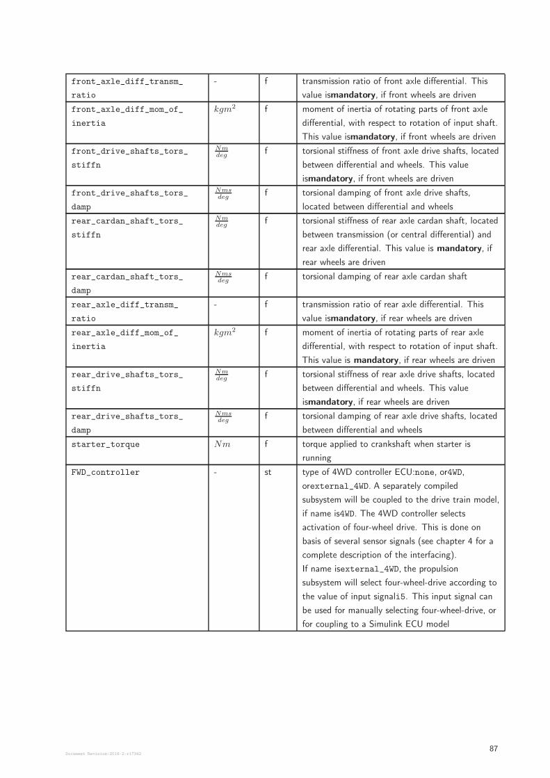
front_axle_diff_transm_
ratio
- f transmission ratio of front axle differential. This
value ismandatory, if front wheels are driven
front_axle_diff_mom_of_
inertia
kgm2 f moment of inertia of rotating parts of front axle
differential, with respect to rotation of input shaft.
This value ismandatory, if front wheels are driven
front_drive_shafts_tors_
stiffn
Nmdeg
f torsional stiffness of front axle drive shafts, located
between differential and wheels. This value
ismandatory, if front wheels are driven
front_drive_shafts_tors_
damp
Nmsdeg
f torsional damping of front axle drive shafts,
located between differential and wheels
rear_cardan_shaft_tors_
stiffn
Nmdeg
f torsional stiffness of rear axle cardan shaft, located
between transmission (or central differential) and
rear axle differential. This value is mandatory, if
rear wheels are driven
rear_cardan_shaft_tors_
damp
Nmsdeg
f torsional damping of rear axle cardan shaft
rear_axle_diff_transm_
ratio
- f transmission ratio of rear axle differential. This
value ismandatory, if rear wheels are driven
rear_axle_diff_mom_of_
inertia
kgm2 f moment of inertia of rotating parts of rear axle
differential, with respect to rotation of input shaft.
This value is mandatory, if rear wheels are driven
rear_drive_shafts_tors_
stiffn
Nmdeg
f torsional stiffness of rear axle drive shafts, located
between differential and wheels. This value
ismandatory, if rear wheels are driven
rear_drive_shafts_tors_
damp
Nmsdeg
f torsional damping of rear axle drive shafts, located
between differential and wheels
starter_torque Nm f torque applied to crankshaft when starter is
running
FWD_controller - st type of 4WD controller ECU:none, or4WD,
orexternal_4WD. A separately compiled
subsystem will be coupled to the drive train model,
if name is4WD. The 4WD controller selects
activation of four-wheel drive. This is done on
basis of several sensor signals (see chapter 4 for a
complete description of the interfacing).
If name isexternal_4WD, the propulsion
subsystem will select four-wheel-drive according to
the value of input signali5. This input signal can
be used for manually selecting four-wheel-drive, or
for coupling to a Simulink ECU model
Document Revision:2018-2-r1734287
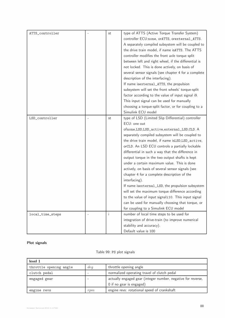
ATTS_controller - st type of ATTS (Active Torque Transfer System)
controller ECU:none, orATTS, orexternal_ATTS.
A separately compiled subsystem will be coupled to
the drive train model, if name isATTS. The ATTS
controller modifies the front axle torque split
between left and right wheel, if the differential is
not locked. This is done actively, on basis of
several sensor signals (see chapter 4 for a complete
description of the interfacing).
If name isexternal_ATTS, the propulsion
subsystem will set the front wheels’ torque-split
factor according to the value of input signal i9.
This input signal can be used for manually
choosing a torque-split factor, or for coupling to a
Simulink ECU model
LSD_controller - st type of LSD (Limited Slip Differential) controller
ECU: one out
ofnone,LSD,LSD_active,external_LSD,CLD. A
separately compiled subsystem will be coupled to
the drive train model, if name isLSD,LSD_active,
orCLD. An LSD ECU controls a partially lockable
differential in such a way that the difference in
output torque in the two output shafts is kept
under a certain maximum value. This is done
actively, on basis of several sensor signals (see
chapter 4 for a complete description of the
interfacing).
If name isexternal_LSD, the propulsion subsystem
will set the maximum torque difference according
to the value of input signali10. This input signal
can be used for manually choosing that torque, or
for coupling to a Simulink ECU model
local_time_steps - i number of local time steps to be used for
integration of drive-train (to improve numerical
stability and accuracy).
Default value is 100
Plot signals
Table 99: PS plot signals
level 1
throttle opening angle deg throttle opening angle
clutch pedal - normalized operating travel of clutch pedal
engaged gear - actually engaged gear (integer number, negative for reverse,
0 if no gear is engaged)
engine revs rpm engine revs: rotational speed of crankshaft
Document Revision:2018-2-r1734288
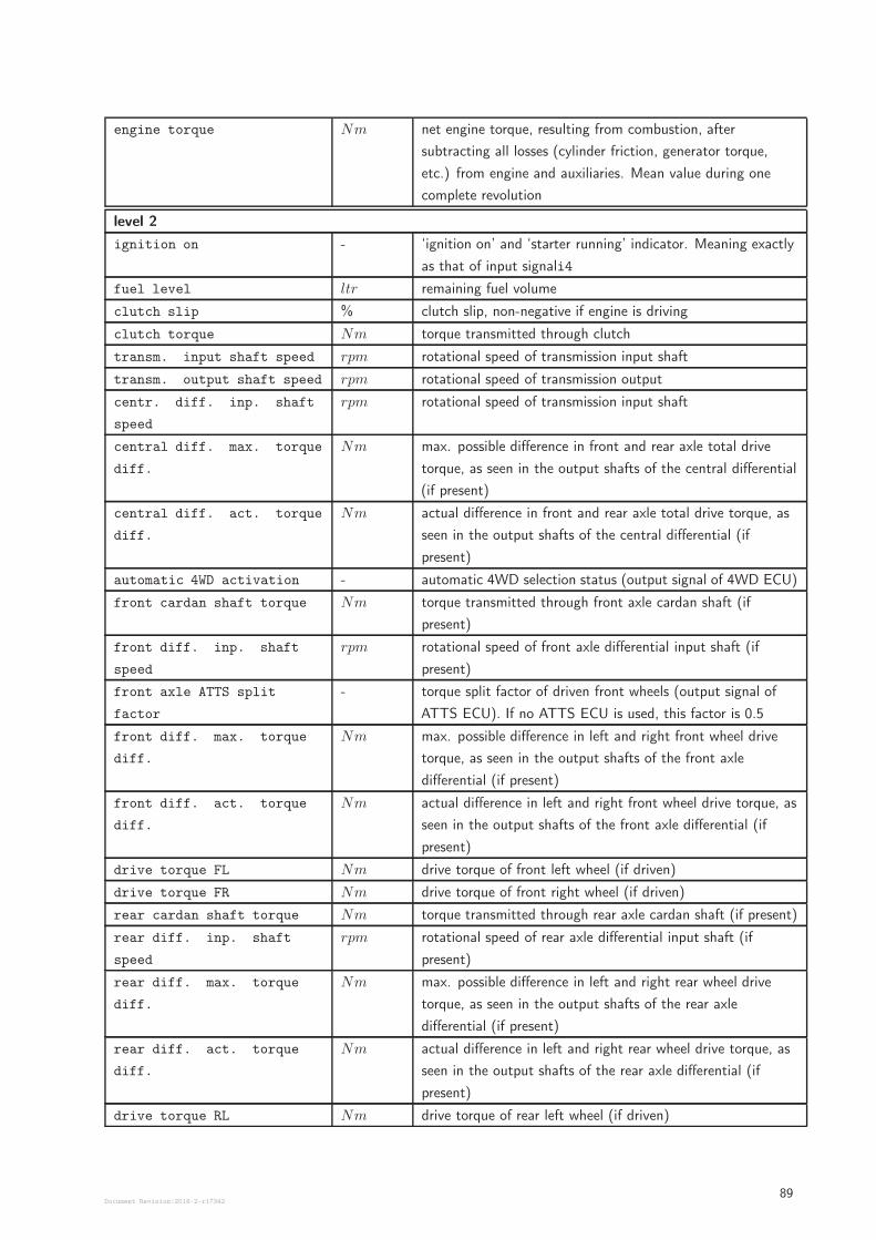
engine torque Nm net engine torque, resulting from combustion, after
subtracting all losses (cylinder friction, generator torque,
etc.) from engine and auxiliaries. Mean value during one
complete revolution
level 2
ignition on - ‘ignition on’ and ‘starter running’ indicator. Meaning exactly
as that of input signali4
fuel level ltr remaining fuel volume
clutch slip % clutch slip, non-negative if engine is driving
clutch torque Nm torque transmitted through clutch
transm. input shaft speed rpm rotational speed of transmission input shaft
transm. output shaft speed rpm rotational speed of transmission output
centr. diff. inp. shaft
speed
rpm rotational speed of transmission input shaft
central diff. max. torque
diff.
Nm max. possible difference in front and rear axle total drive
torque, as seen in the output shafts of the central differential
(if present)
central diff. act. torque
diff.
Nm actual difference in front and rear axle total drive torque, as
seen in the output shafts of the central differential (if
present)
automatic 4WD activation - automatic 4WD selection status (output signal of 4WD ECU)
front cardan shaft torque Nm torque transmitted through front axle cardan shaft (if
present)
front diff. inp. shaft
speed
rpm rotational speed of front axle differential input shaft (if
present)
front axle ATTS split
factor
- torque split factor of driven front wheels (output signal of
ATTS ECU). If no ATTS ECU is used, this factor is 0.5
front diff. max. torque
diff.
Nm max. possible difference in left and right front wheel drive
torque, as seen in the output shafts of the front axle
differential (if present)
front diff. act. torque
diff.
Nm actual difference in left and right front wheel drive torque, as
seen in the output shafts of the front axle differential (if
present)
drive torque FL Nm drive torque of front left wheel (if driven)
drive torque FR Nm drive torque of front right wheel (if driven)
rear cardan shaft torque Nm torque transmitted through rear axle cardan shaft (if present)
rear diff. inp. shaft
speed
rpm rotational speed of rear axle differential input shaft (if
present)
rear diff. max. torque
diff.
Nm max. possible difference in left and right rear wheel drive
torque, as seen in the output shafts of the rear axle
differential (if present)
rear diff. act. torque
diff.
Nm actual difference in left and right rear wheel drive torque, as
seen in the output shafts of the rear axle differential (if
present)
drive torque RL Nm drive torque of rear left wheel (if driven)
Document Revision:2018-2-r1734289
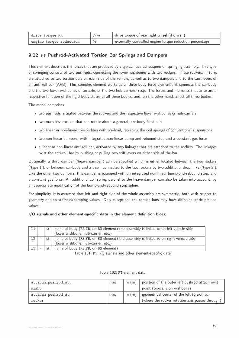
drive torque RR Nm drive torque of rear right wheel (if driven)
engine torque reduction % externally controlled engine torque reduction percentage
9.22 PT Pushrod-Activated Torsion Bar Springs and Dampers
This element describes the forces that are produced by a typical race-car suspension springing assembly. This type
of springing consists of two pushrods, connecting the lower wishbones with two rockers. These rockers, in turn,
are attached to two torsion bars on each side of the vehicle, as well as to two dampers and to the cantilevers of
an anti-roll bar (ARB). This complex element works as a ‘three-body force element’: it connects the car-body
and the two lower wishbones of an axle, or the two hub-carriers, resp. The forces and moments that arise are a
respective function of the rigid-body states of all three bodies, and, on the other hand, affect all three bodies.
The model comprises
• two pushrods, situated between the rockers and the respective lower wishbones or hub-carriers
• two mass-less rockers that can rotate about a general, car-body-fixed axis
• two linear or non-linear torsion bars with pre-load, replacing the coil springs of conventional suspensions
• two non-linear dampers, with integrated non-linear bump-and-rebound stop and a constant gas force
• a linear or non-linear anti-roll bar, activated by two linkages that are attached to the rockers. The linkages
twist the anti-roll bar by pushing or pulling two stiff levers on either side of the bar.
Optionally, a third damper (‘heave damper’) can be specified which is either located between the two rockers
(‘type 1’), or between car-body and a beam connected to the two rockers by two additional drop links (‘type 2’).
Like the other two dampers, this damper is equipped with an integrated non-linear bump-and-rebound stop, and
a constant gas force. An additional coil spring parallel to the heave damper can also be taken into account, by
an appropriate modification of the bump-and-rebound stop spline.
For simplicity, it is assumed that left and right side of the whole assembly are symmetric, both with respect to
geometry and to stiffness/damping values. Only exception: the torsion bars may have different static preload
values.
I/O signals and other element-specific data in the element definition block
l1 - st name of body (RB,FB, or BO element) the assembly is linked to on left vehicle side(lower wishbone, hub-carrier, etc.)
l2 - st name of body (RB,FB, or BO element) the assembly is linked to on right vehicle side(lower wishbone, hub-carrier, etc.)
l3 - st name of body (RB,FB, or BO element)Table 101: PT I/O signals and other element-specific data
Table 102: PT element data
attachm_pushrod_at_
wishb
mm m (m) position of the outer left pushrod attachment
point (typically on wishbone)
attachm_pushrod_at_
rocker
mm m (m) geometrical center of the left torsion bar
(where the rocker rotation axis passes through)
Document Revision:2018-2-r1734290
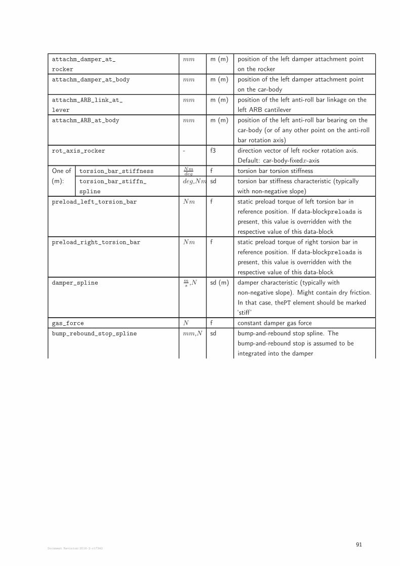
attachm_damper_at_
rocker
mm m (m) position of the left damper attachment point
on the rocker
attachm_damper_at_body mm m (m) position of the left damper attachment point
on the car-body
attachm_ARB_link_at_
lever
mm m (m) position of the left anti-roll bar linkage on the
left ARB cantilever
attachm_ARB_at_body mm m (m) position of the left anti-roll bar bearing on the
car-body (or of any other point on the anti-roll
bar rotation axis)
rot_axis_rocker - f3 direction vector of left rocker rotation axis.
Default: car-body-fixedx-axis
One of
(m):
torsion_bar_stiffness Nmdeg
f torsion bar torsion stiffness
torsion_bar_stiffn_
spline
deg,Nm sd torsion bar stiffness characteristic (typically
with non-negative slope)
preload_left_torsion_bar Nm f static preload torque of left torsion bar in
reference position. If data-blockpreloads is
present, this value is overridden with the
respective value of this data-block
preload_right_torsion_bar Nm f static preload torque of right torsion bar in
reference position. If data-blockpreloads is
present, this value is overridden with the
respective value of this data-block
damper_spline ms,N sd (m) damper characteristic (typically with
non-negative slope). Might contain dry friction.
In that case, thePT element should be marked
‘stiff’
gas_force N f constant damper gas force
bump_rebound_stop_spline mm,N sd bump-and-rebound stop spline. The
bump-and-rebound stop is assumed to be
integrated into the damper
Document Revision:2018-2-r1734291
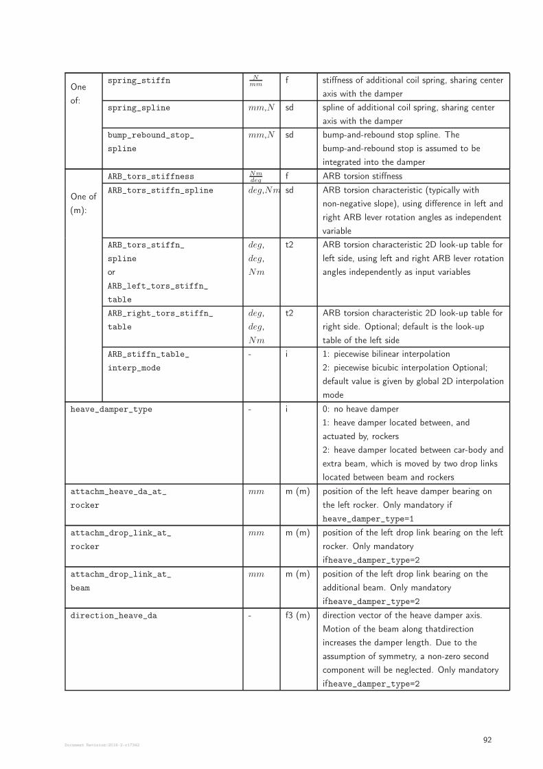
One
of:
spring_stiffn Nmm
f stiffness of additional coil spring, sharing center
axis with the damper
spring_spline mm,N sd spline of additional coil spring, sharing center
axis with the damper
bump_rebound_stop_
spline
mm,N sd bump-and-rebound stop spline. The
bump-and-rebound stop is assumed to be
integrated into the damper
One of
(m):
ARB_tors_stiffness Nmdeg
f ARB torsion stiffness
ARB_tors_stiffn_spline deg,Nm sd ARB torsion characteristic (typically with
non-negative slope), using difference in left and
right ARB lever rotation angles as independent
variable
ARB_tors_stiffn_
spline
or
ARB_left_tors_stiffn_
table
deg,
deg,
Nm
t2 ARB torsion characteristic 2D look-up table for
left side, using left and right ARB lever rotation
angles independently as input variables
ARB_right_tors_stiffn_
table
deg,
deg,
Nm
t2 ARB torsion characteristic 2D look-up table for
right side. Optional; default is the look-up
table of the left side
ARB_stiffn_table_
interp_mode
- i 1: piecewise bilinear interpolation
2: piecewise bicubic interpolation Optional;
default value is given by global 2D interpolation
mode
heave_damper_type - i 0: no heave damper
1: heave damper located between, and
actuated by, rockers
2: heave damper located between car-body and
extra beam, which is moved by two drop links
located between beam and rockers
attachm_heave_da_at_
rocker
mm m (m) position of the left heave damper bearing on
the left rocker. Only mandatory if
heave_damper_type=1
attachm_drop_link_at_
rocker
mm m (m) position of the left drop link bearing on the left
rocker. Only mandatory
ifheave_damper_type=2
attachm_drop_link_at_
beam
mm m (m) position of the left drop link bearing on the
additional beam. Only mandatory
ifheave_damper_type=2
direction_heave_da - f3 (m) direction vector of the heave damper axis.
Motion of the beam along thatdirection
increases the damper length. Due to the
assumption of symmetry, a non-zero second
component will be neglected. Only mandatory
ifheave_damper_type=2
Document Revision:2018-2-r1734292
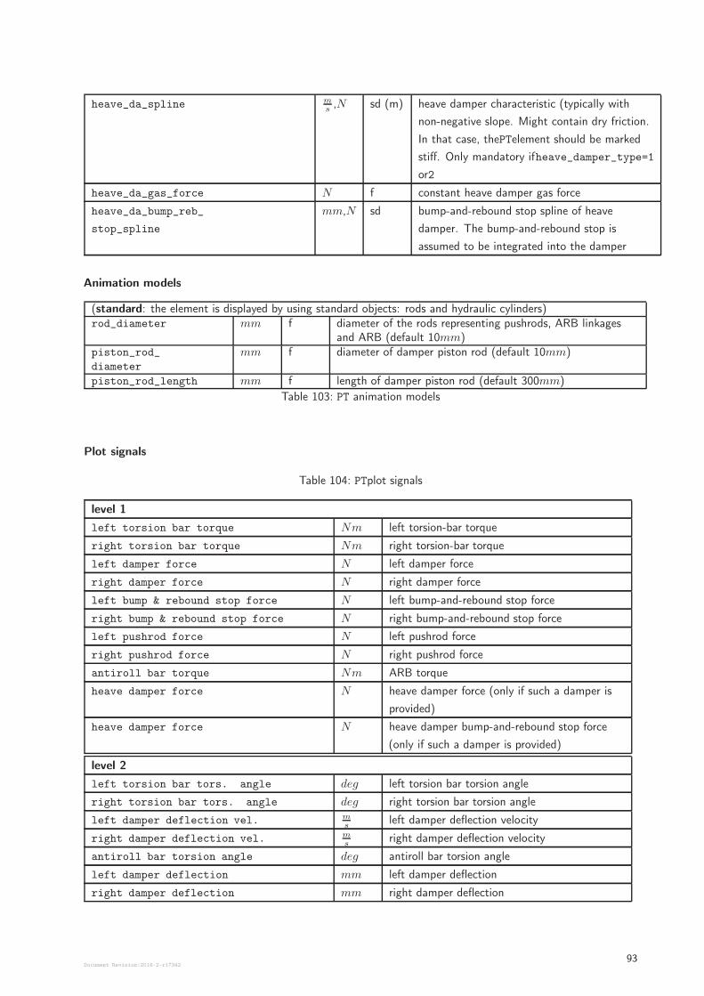
heave_da_spline ms,N sd (m) heave damper characteristic (typically with
non-negative slope. Might contain dry friction.
In that case, thePTelement should be marked
stiff. Only mandatory ifheave_damper_type=1
or2
heave_da_gas_force N f constant heave damper gas force
heave_da_bump_reb_
stop_spline
mm,N sd bump-and-rebound stop spline of heave
damper. The bump-and-rebound stop is
assumed to be integrated into the damper
Animation models
(standard: the element is displayed by using standard objects: rods and hydraulic cylinders)rod_diameter mm f diameter of the rods representing pushrods, ARB linkages
and ARB (default 10mm)piston_rod_
diameter
mm f diameter of damper piston rod (default 10mm)
piston_rod_length mm f length of damper piston rod (default 300mm)
Table 103: PT animation models
Plot signals
Table 104: PTplot signals
level 1
left torsion bar torque Nm left torsion-bar torque
right torsion bar torque Nm right torsion-bar torque
left damper force N left damper force
right damper force N right damper force
left bump & rebound stop force N left bump-and-rebound stop force
right bump & rebound stop force N right bump-and-rebound stop force
left pushrod force N left pushrod force
right pushrod force N right pushrod force
antiroll bar torque Nm ARB torque
heave damper force N heave damper force (only if such a damper is
provided)
heave damper force N heave damper bump-and-rebound stop force
(only if such a damper is provided)
level 2
left torsion bar tors. angle deg left torsion bar torsion angle
right torsion bar tors. angle deg right torsion bar torsion angle
left damper deflection vel. ms
left damper deflection velocity
right damper deflection vel. ms
right damper deflection velocity
antiroll bar torsion angle deg antiroll bar torsion angle
left damper deflection mm left damper deflection
right damper deflection mm right damper deflection
Document Revision:2018-2-r1734293
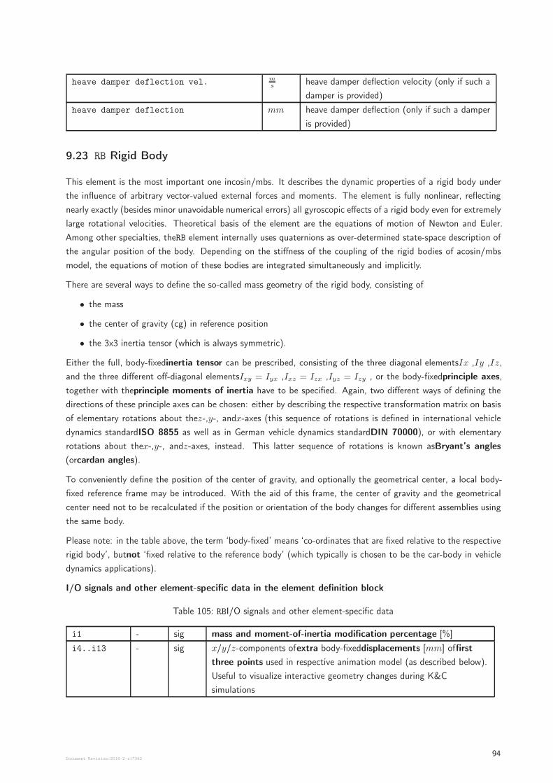
heave damper deflection vel. ms
heave damper deflection velocity (only if such a
damper is provided)
heave damper deflection mm heave damper deflection (only if such a damper
is provided)
9.23 RB Rigid Body
This element is the most important one incosin/mbs. It describes the dynamic properties of a rigid body under
the influence of arbitrary vector-valued external forces and moments. The element is fully nonlinear, reflecting
nearly exactly (besides minor unavoidable numerical errors) all gyroscopic effects of a rigid body even for extremely
large rotational velocities. Theoretical basis of the element are the equations of motion of Newton and Euler.
Among other specialties, theRB element internally uses quaternions as over-determined state-space description of
the angular position of the body. Depending on the stiffness of the coupling of the rigid bodies of acosin/mbs
model, the equations of motion of these bodies are integrated simultaneously and implicitly.
There are several ways to define the so-called mass geometry of the rigid body, consisting of
• the mass
• the center of gravity (cg) in reference position
• the 3x3 inertia tensor (which is always symmetric).
Either the full, body-fixedinertia tensor can be prescribed, consisting of the three diagonal elementsIx ,Iy ,Iz,
and the three different off-diagonal elementsIxy = Iyx ,Ixz = Izx ,Iyz = Izy , or the body-fixedprinciple axes,
together with theprinciple moments of inertia have to be specified. Again, two different ways of defining the
directions of these principle axes can be chosen: either by describing the respective transformation matrix on basis
of elementary rotations about thez-,y-, andx-axes (this sequence of rotations is defined in international vehicle
dynamics standardISO 8855 as well as in German vehicle dynamics standardDIN 70000), or with elementary
rotations about thex-,y-, andz-axes, instead. This latter sequence of rotations is known asBryant’s angles
(orcardan angles).
To conveniently define the position of the center of gravity, and optionally the geometrical center, a local body-
fixed reference frame may be introduced. With the aid of this frame, the center of gravity and the geometrical
center need not to be recalculated if the position or orientation of the body changes for different assemblies using
the same body.
Please note: in the table above, the term ‘body-fixed’ means ‘co-ordinates that are fixed relative to the respective
rigid body’, butnot ‘fixed relative to the reference body’ (which typically is chosen to be the car-body in vehicle
dynamics applications).
I/O signals and other element-specific data in the element definition block
Table 105: RBI/O signals and other element-specific data
i1 - sig mass and moment-of-inertia modification percentage [%]
i4..i13 - sig x/y/z-components ofextra body-fixeddisplacements [mm] offirst
three points used in respective animation model (as described below).
Useful to visualize interactive geometry changes during K&C
simulations
Document Revision:2018-2-r1734294
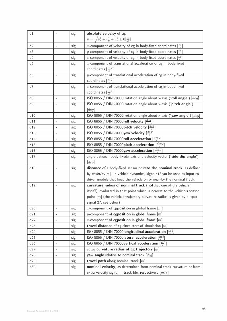
o1 - sig absolute velocity of cg:
v =√
v2x + v2y + v2z ≥ 0[ms]
o2 - sig x-component of velocity of cg in body-fixed coordinates [ms]
o3 - sig y-component of velocity of cg in body-fixed coordinates [ms]
o4 - sig z-component of velocity of cg in body-fixed coordinates [ms]
o5 - sig x-component of translational acceleration of cg in body-fixed
coordinates [ms2]
o6 - sig y-component of translational acceleration of cg in body-fixed
coordinates [ms2]
o7 - sig z-component of translational acceleration of cg in body-fixed
coordinates [ms2]
o8 - sig ISO 8855 / DIN 70000 rotation angle about x-axis (‘roll angle’) [deg]
o9 - sig ISO 8855 / DIN 70000 rotation angle about x-axis (‘pitch angle’)
[deg]
o10 - sig ISO 8855 / DIN 70000 rotation angle about x-axis (‘yaw angle’) [deg]
o11 - sig ISO 8855 / DIN 70000roll velocity [degs
]
o12 - sig ISO 8855 / DIN 70000pitch velocity [degs
]
o13 - sig ISO 8855 / DIN 70000yaw velocity [degs
]
o14 - sig ISO 8855 / DIN 70000roll acceleration [degs
2]
o15 - sig ISO 8855 / DIN 70000pitch acceleration [degs
2]
o16 - sig ISO 8855 / DIN 70000yaw acceleration [degs
2]
o17 - sig angle between body-fixedx-axis and velocity vector (‘side-slip angle’)
[deg]
o18 - sig distance of a body-fixed sensor pointto the nominal track, as defined
by cosin/ev [m]. In vehicle dynamics, signalo18can be used as input to
driver models that keep the vehicle on or near-by the nominal track.
o19 - sig curvature radius of nominal track (notthat one of the vehicle
itself!), evaluated in that point which is nearest to the vehicle’s sensor
point [m] (the vehicle’s trajectory curvature radius is given by output
signal 27, see below)
o20 - sig x-component of cgposition in global frame [m]
o21 - sig y-component of cgposition in global frame [m]
o22 - sig z-component of cgposition in global frame [m]
o23 - sig travel distance of cg since start of simulation [m]
o24 - sig ISO 8855 / DIN 70000longitudinal acceleration [ms2]
o25 - sig ISO 8855 / DIN 70000lateral acceleration [ms2]
o26 - sig ISO 8855 / DIN 70000vertical acceleration [ms2]
o27 - sig actualcurvature radius of cg trajectory [m]
o28 - sig yaw angle relative to nominal track [deg]
o29 - sig travel path along nominal track [m]
o30 - sig nominal velocity, as determined from nominal track curvature or from
extra velocity signal in track file, respectively [m/s]
Document Revision:2018-2-r1734295
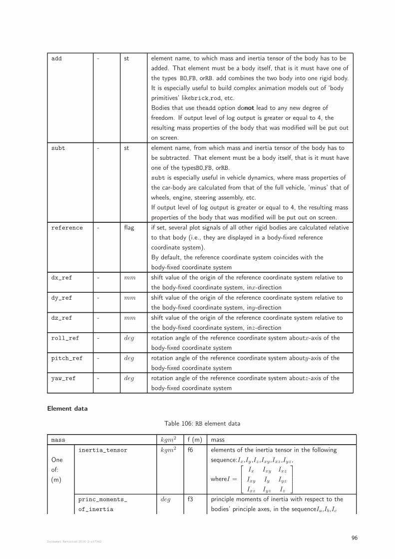
add - st element name, to which mass and inertia tensor of the body has to be
added. That element must be a body itself, that is it must have one of
the types BO,FB, orRB. add combines the two body into one rigid body.
It is especially useful to build complex animation models out of ‘body
primitives’ likebrick,rod, etc.
Bodies that use theadd option donot lead to any new degree of
freedom. If output level of log output is greater or equal to 4, the
resulting mass properties of the body that was modified will be put out
on screen.
subt - st element name, from which mass and inertia tensor of the body has to
be subtracted. That element must be a body itself, that is it must have
one of the typesBO,FB, orRB.
subt is especially useful in vehicle dynamics, where mass properties of
the car-body are calculated from that of the full vehicle, ‘minus’ that of
wheels, engine, steering assembly, etc.
If output level of log output is greater or equal to 4, the resulting mass
properties of the body that was modified will be put out on screen.
reference - flag if set, several plot signals of all other rigid bodies are calculated relative
to that body (i.e., they are displayed in a body-fixed reference
coordinate system).
By default, the reference coordinate system coincides with the
body-fixed coordinate system
dx_ref - mm shift value of the origin of the reference coordinate system relative to
the body-fixed coordinate system, inx-direction
dy_ref - mm shift value of the origin of the reference coordinate system relative to
the body-fixed coordinate system, iny-direction
dz_ref - mm shift value of the origin of the reference coordinate system relative to
the body-fixed coordinate system, inz-direction
roll_ref - deg rotation angle of the reference coordinate system aboutx-axis of the
body-fixed coordinate system
pitch_ref - deg rotation angle of the reference coordinate system abouty-axis of the
body-fixed coordinate system
yaw_ref - deg rotation angle of the reference coordinate system aboutz-axis of the
body-fixed coordinate system
Element data
Table 106: RB element data
mass kgm2 f (m) mass
One
of:
(m)
inertia_tensor kgm2 f6 elements of the inertia tensor in the following
sequence:Ix,Iy,Iz ,Ixy,Ixz ,Iyz,
whereI =
Ix Ixy Ixz
Ixy Iy Iyz
Ixz Iyz Iz
princ_moments_
of_inertia
deg f3 principle moments of inertia with respect to the
bodies’ principle axes, in the sequenceIa,Ib,Ic
Document Revision:2018-2-r1734296
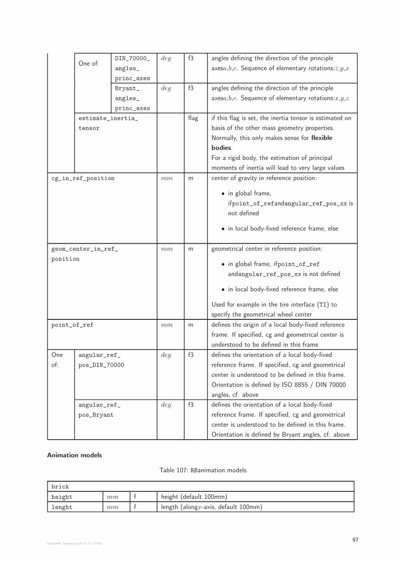
One of:DIN_70000_
angles_
princ_axes
deg f3 angles defining the direction of the principle
axesa,b,c. Sequence of elementary rotations:z,y,x
Bryant_
angles_
princ_axes
deg f3 angles defining the direction of the principle
axesa,b,c. Sequence of elementary rotations:x,y,z
estimate_inertia_
tensor
flag if this flag is set, the inertia tensor is estimated on
basis of the other mass geometry properties.
Normally, this only makes sense for flexible
bodies.
For a rigid body, the estimation of principal
moments of inertia will lead to very large values
cg_in_ref_position mm m center of gravity in reference position:
• in global frame,
ifpoint_of_refandangular_ref_pos_xx is
not defined
• in local body-fixed reference frame, else
geom_center_in_ref_
position
mm m geometrical center in reference position:
• in global frame, ifpoint_of_ref
andangular_ref_pos_xx is not defined
• in local body-fixed reference frame, else
Used for example in the tire interface (TI) to
specify the geometrical wheel center
point_of_ref mm m defines the origin of a local body-fixed reference
frame. If specified, cg and geometrical center is
understood to be defined in this frame
One
of:
angular_ref_
pos_DIN_70000
deg f3 defines the orientation of a local body-fixed
reference frame. If specified, cg and geometrical
center is understood to be defined in this frame.
Orientation is defined by ISO 8855 / DIN 70000
angles, cf. above
angular_ref_
pos_Bryant
deg f3 defines the orientation of a local body-fixed
reference frame. If specified, cg and geometrical
center is understood to be defined in this frame.
Orientation is defined by Bryant angles, cf. above
Animation models
Table 107: RBanimation models
brick
height mm f height (default 100mm)
lenght mm f length (alongx-axis, default 100mm)
Document Revision:2018-2-r1734297
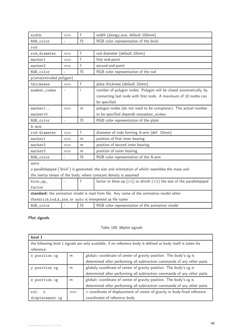
width mm f width (alongy-axis, default 100mm)
RGB_color - f3 RGB color representation of the brick
rod
rod_diameter mm f rod diameter (default 10mm)
marker1 mm f first end-point
marker2 mm f second end-point
RGB_color - f3 RGB color representation of the rod
plate(extruded polygon)
thickness mm f plate thickness (default 10mm)
number_codes - i number of polygon nodes. Polygon will be closed automatically, by
connecting last node with first node. A maximum of 10 nodes can
be specified
marker1..
marker10
mm m polygon nodes (do not need to be complanar). The actual number
to be specified depends onnumber_nodes
RGB_color - f3 RGB color representation of the plate
A-arm
rod-diameter mm f diameter of rods forming A-arm (def. 10mm)
marker1 mm m position of first inner bearing
marker2 mm m position of second inner bearing
marker3 mm m position of outer bearing
RGB_color - f3 RGB color representation of the A-arm
auto
a parallelepiped (’brick’) is generated, the size and orientation of which resembles the mass and
the inertia tensor of the body, where constant density is assumed
blow_up_
factor
- f factor to blow-up (>1) or shrink (<1) the size of the parallelepiped
standard: the animation model is read from file. Any name of the animation model other
thanbrick,rod,A_arm, or auto is interpreted as file name
RGB_color - f3 RGB color representation of the animation model
Plot signals
Table 108: RBplot signals
level 1
the following level 1 signals are only available, if no reference body is defined or body itself is taken for
reference:
x position cg m globalx coordinate of center of gravity position. The body’s cg is
determined after performing all subtraction commands of any other parts
y position cg m globaly coordinate of center of gravity position. The body’s cg is
determined after performing all subtraction commands of any other parts
z position cg m globalz coordinate of center of gravity position. The body’s cg is
determined after performing all subtraction commands of any other parts
rel. x
displacement cg
mm x coordinate of displacement of center of gravity in body-fixed reference
coordinates of reference body
Document Revision:2018-2-r1734298
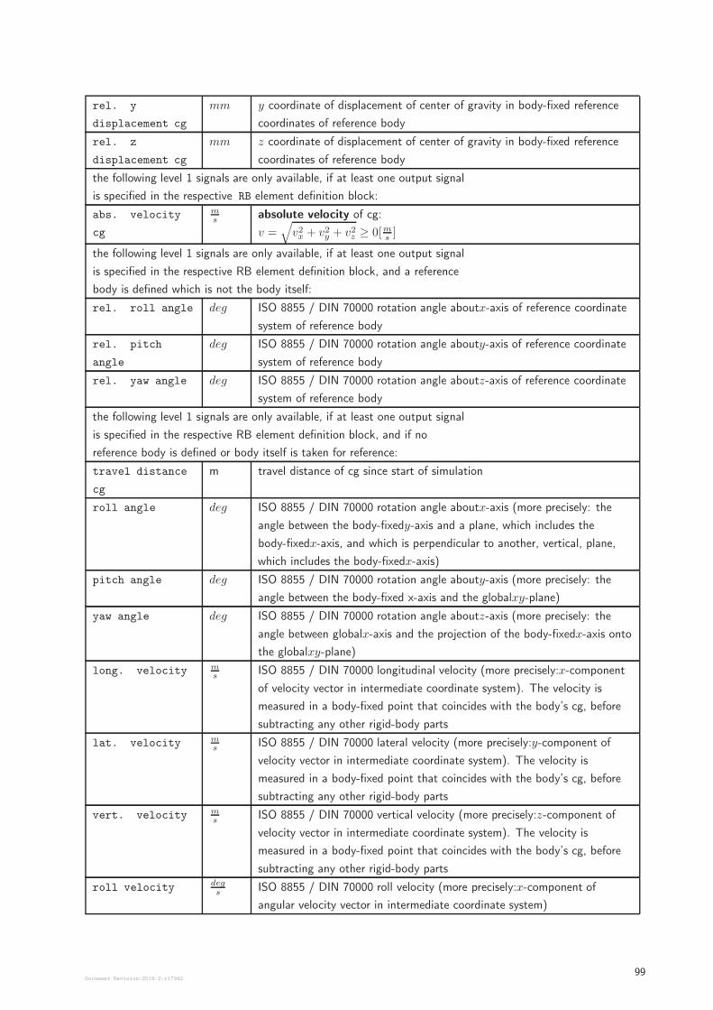
rel. y
displacement cg
mm y coordinate of displacement of center of gravity in body-fixed reference
coordinates of reference body
rel. z
displacement cg
mm z coordinate of displacement of center of gravity in body-fixed reference
coordinates of reference body
the following level 1 signals are only available, if at least one output signal
is specified in the respective RB element definition block:
abs. velocity
cg
ms
absolute velocity of cg:
v =√
v2x + v2y + v2z ≥ 0[ms]
the following level 1 signals are only available, if at least one output signal
is specified in the respective RB element definition block, and a reference
body is defined which is not the body itself:
rel. roll angle deg ISO 8855 / DIN 70000 rotation angle aboutx-axis of reference coordinate
system of reference body
rel. pitch
angle
deg ISO 8855 / DIN 70000 rotation angle abouty-axis of reference coordinate
system of reference body
rel. yaw angle deg ISO 8855 / DIN 70000 rotation angle aboutz-axis of reference coordinate
system of reference body
the following level 1 signals are only available, if at least one output signal
is specified in the respective RB element definition block, and if no
reference body is defined or body itself is taken for reference:
travel distance
cg
m travel distance of cg since start of simulation
roll angle deg ISO 8855 / DIN 70000 rotation angle aboutx-axis (more precisely: the
angle between the body-fixedy-axis and a plane, which includes the
body-fixedx-axis, and which is perpendicular to another, vertical, plane,
which includes the body-fixedx-axis)
pitch angle deg ISO 8855 / DIN 70000 rotation angle abouty-axis (more precisely: the
angle between the body-fixed x-axis and the globalxy-plane)
yaw angle deg ISO 8855 / DIN 70000 rotation angle aboutz-axis (more precisely: the
angle between globalx-axis and the projection of the body-fixedx-axis onto
the globalxy-plane)
long. velocity ms
ISO 8855 / DIN 70000 longitudinal velocity (more precisely:x-component
of velocity vector in intermediate coordinate system). The velocity is
measured in a body-fixed point that coincides with the body’s cg, before
subtracting any other rigid-body parts
lat. velocity ms
ISO 8855 / DIN 70000 lateral velocity (more precisely:y-component of
velocity vector in intermediate coordinate system). The velocity is
measured in a body-fixed point that coincides with the body’s cg, before
subtracting any other rigid-body parts
vert. velocity ms
ISO 8855 / DIN 70000 vertical velocity (more precisely:z-component of
velocity vector in intermediate coordinate system). The velocity is
measured in a body-fixed point that coincides with the body’s cg, before
subtracting any other rigid-body parts
roll velocity degs
ISO 8855 / DIN 70000 roll velocity (more precisely:x-component of
angular velocity vector in intermediate coordinate system)
Document Revision:2018-2-r1734299
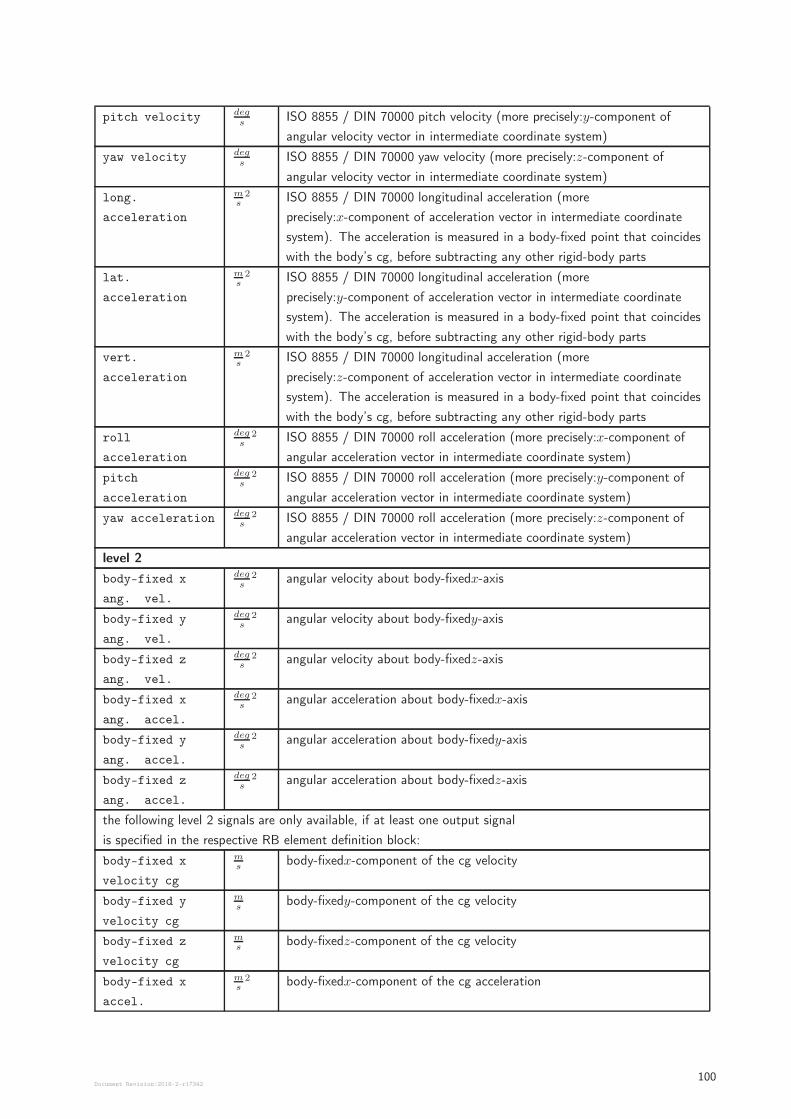
pitch velocity degs
ISO 8855 / DIN 70000 pitch velocity (more precisely:y-component of
angular velocity vector in intermediate coordinate system)
yaw velocity degs
ISO 8855 / DIN 70000 yaw velocity (more precisely:z-component of
angular velocity vector in intermediate coordinate system)
long.
acceleration
ms2 ISO 8855 / DIN 70000 longitudinal acceleration (more
precisely:x-component of acceleration vector in intermediate coordinate
system). The acceleration is measured in a body-fixed point that coincides
with the body’s cg, before subtracting any other rigid-body parts
lat.
acceleration
ms2 ISO 8855 / DIN 70000 longitudinal acceleration (more
precisely:y-component of acceleration vector in intermediate coordinate
system). The acceleration is measured in a body-fixed point that coincides
with the body’s cg, before subtracting any other rigid-body parts
vert.
acceleration
ms2 ISO 8855 / DIN 70000 longitudinal acceleration (more
precisely:z-component of acceleration vector in intermediate coordinate
system). The acceleration is measured in a body-fixed point that coincides
with the body’s cg, before subtracting any other rigid-body parts
roll
acceleration
degs
2 ISO 8855 / DIN 70000 roll acceleration (more precisely:x-component of
angular acceleration vector in intermediate coordinate system)
pitch
acceleration
degs
2 ISO 8855 / DIN 70000 roll acceleration (more precisely:y-component of
angular acceleration vector in intermediate coordinate system)
yaw acceleration degs
2 ISO 8855 / DIN 70000 roll acceleration (more precisely:z-component of
angular acceleration vector in intermediate coordinate system)
level 2
body-fixed x
ang. vel.
degs
2 angular velocity about body-fixedx-axis
body-fixed y
ang. vel.
degs
2 angular velocity about body-fixedy-axis
body-fixed z
ang. vel.
degs
2 angular velocity about body-fixedz-axis
body-fixed x
ang. accel.
degs
2 angular acceleration about body-fixedx-axis
body-fixed y
ang. accel.
degs
2 angular acceleration about body-fixedy-axis
body-fixed z
ang. accel.
degs
2 angular acceleration about body-fixedz-axis
the following level 2 signals are only available, if at least one output signal
is specified in the respective RB element definition block:
body-fixed x
velocity cg
ms
body-fixedx-component of the cg velocity
body-fixed y
velocity cg
ms
body-fixedy-component of the cg velocity
body-fixed z
velocity cg
ms
body-fixedz-component of the cg velocity
body-fixed x
accel.
ms2 body-fixedx-component of the cg acceleration
Document Revision:2018-2-r17342100
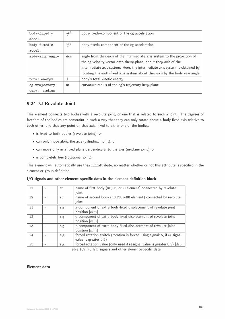
body-fixed y
accel.
ms2 body-fixedy-component of the cg acceleration
body-fixed z
accel.
ms2 body-fixedz-component of the cg acceleration
side-slip angle deg angle from thex-axis of the intermediate axis system to the projection of
the cg velocity vector onto thexy-plane, about they-axis of the
intermediate axis system. Here, the intermediate axis system is obtained by
rotating the earth-fixed axis system about thez-axis by the body yaw angle
total energy J body’s total kinetic energy
cg trajectory
curv. radius
m curvature radius of the cg’s trajectory inxy-plane
9.24 RJ Revolute Joint
This element connects two bodies with a revolute joint, or one that is related to such a joint. The degrees of
freedom of the bodies are constraint in such a way that they can only rotate about a body-fixed axis relative to
each other, and that any point on that axis, fixed to either one of the bodies,
• is fixed to both bodies (revolute joint), or
• can only move along the axis (cylindrical joint), or
• can move only in a fixed plane perpendicular to the axis (in-plane joint), or
• is completely free (rotational joint).
This element will automatically use thestiffattribute, no matter whether or not this attribute is specified in the
element or group definition.
I/O signals and other element-specific data in the element definition block
l1 - st name of first body (RB,FB, orBO element) connected by revolutejoint
l2 - st name of second body (RB,FB, orBO element) connected by revolutejoint
i1 - sig x-component of extra body-fixed displacement of revolute jointposition [mm]
i2 - sig y-component of extra body-fixed displacement of revolute jointposition [mm]
i3 - sig z-component of extra body-fixed displacement of revolute jointposition [mm]
i4 - sig forced rotation switch (rotation is forced using signali5, ifi4 signalvalue is greater 0.5)
i5 - sig forced rotation value (only used ifi4signal value is greater 0.5) [deg]
Table 109: RJ I/O signals and other element-specific data
Element data
Document Revision:2018-2-r17342101
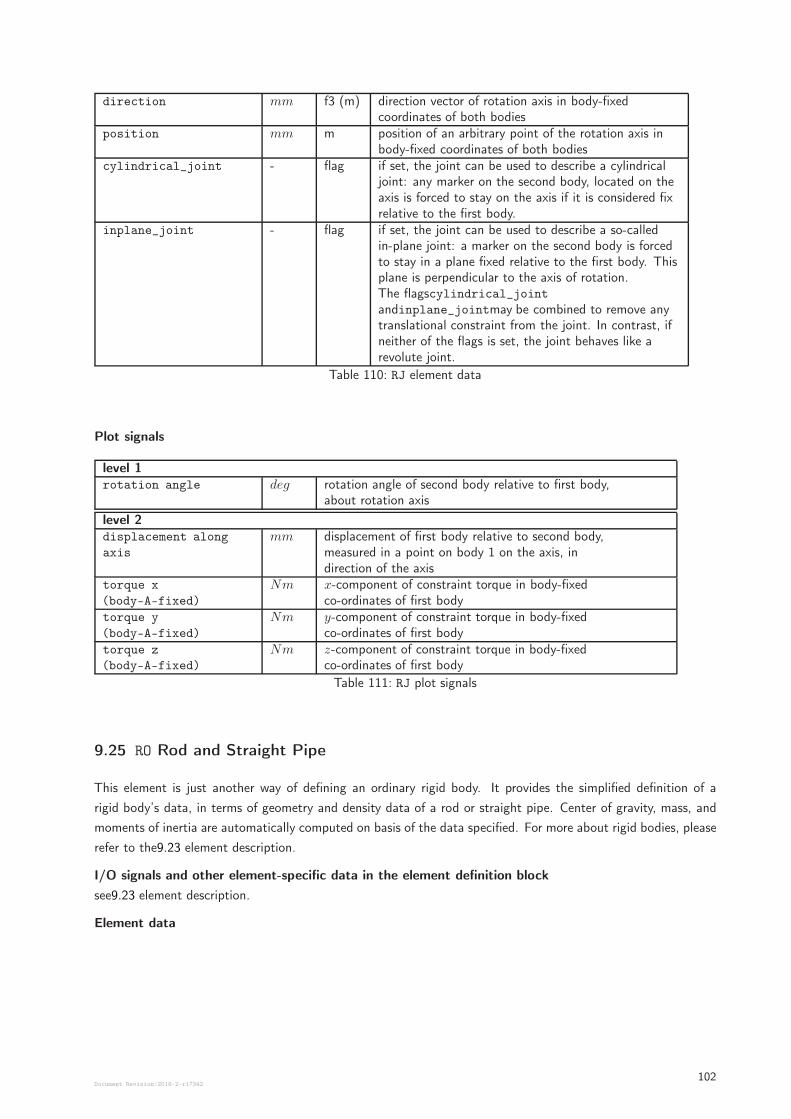
direction mm f3 (m) direction vector of rotation axis in body-fixedcoordinates of both bodies
position mm m position of an arbitrary point of the rotation axis inbody-fixed coordinates of both bodies
cylindrical_joint - flag if set, the joint can be used to describe a cylindricaljoint: any marker on the second body, located on theaxis is forced to stay on the axis if it is considered fixrelative to the first body.
inplane_joint - flag if set, the joint can be used to describe a so-calledin-plane joint: a marker on the second body is forcedto stay in a plane fixed relative to the first body. Thisplane is perpendicular to the axis of rotation.The flagscylindrical_jointandinplane_jointmay be combined to remove anytranslational constraint from the joint. In contrast, ifneither of the flags is set, the joint behaves like arevolute joint.
Table 110: RJ element data
Plot signals
level 1rotation angle deg rotation angle of second body relative to first body,
about rotation axis
level 2displacement along
axis
mm displacement of first body relative to second body,measured in a point on body 1 on the axis, indirection of the axis
torque x
(body-A-fixed)
Nm x-component of constraint torque in body-fixedco-ordinates of first body
torque y
(body-A-fixed)
Nm y-component of constraint torque in body-fixedco-ordinates of first body
torque z
(body-A-fixed)
Nm z-component of constraint torque in body-fixedco-ordinates of first body
Table 111: RJ plot signals
9.25 RO Rod and Straight Pipe
This element is just another way of defining an ordinary rigid body. It provides the simplified definition of a
rigid body’s data, in terms of geometry and density data of a rod or straight pipe. Center of gravity, mass, and
moments of inertia are automatically computed on basis of the data specified. For more about rigid bodies, please
refer to the9.23 element description.
I/O signals and other element-specific data in the element definition block
see9.23 element description.
Element data
Document Revision:2018-2-r17342102
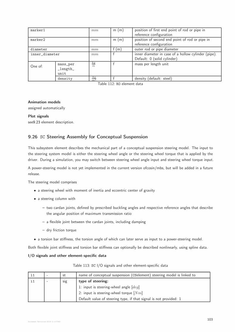
marker1 mm m (m) position of first end point of rod or pipe inreference configuration
marker2 mm m (m) position of second end point of rod or pipe inreference configuration
diameter mm f (m) outer rod or pipe diameterinner_diameter mm f inner diameter in case of a hollow cylinder (pipe).
Default: 0 (solid cylinder)
One of:mass_per
_length_
unit
kgm
f mass per length unit
density kgm3 f density (default: steel)
Table 112: RO element data
Animation models
assigned automatically
Plot signals
see9.23 element description.
9.26 SC Steering Assembly for Conceptual Suspension
This subsystem element describes the mechanical part of a conceptual suspension steering model. The input to
the steering system model is either the steering wheel angle or the steering wheel torque that is applied by the
driver. During a simulation, you may switch between steering wheel angle input and steering wheel torque input.
A power-steering model is not yet implemented in the current version ofcosin/mbs, but will be added in a future
release.
The steering model comprises
• a steering wheel with moment of inertia and eccentric center of gravity
• a steering column with
– two cardan joints, defined by prescribed buckling angles and respective reference angles that describe
the angular position of maximum transmission ratio
– a flexible joint between the cardan joints, including damping
– dry friction torque
• a torsion bar stiffness, the torsion angle of which can later serve as input to a power-steering model.
Both flexible joint stiffness and torsion bar stiffness can optionally be described nonlinearly, using spline data.
I/O signals and other element-specific data
Table 113: SC I/O signals and other element-specific data
l1 - st name of conceptual suspension (CSelement) steering model is linked to
i1 - sig type of steering:
1: input is steering-wheel angle [deg]
2: input is steering-wheel torque [Nm]
Default value of steering type, if that signal is not provided: 1
Document Revision:2018-2-r17342103
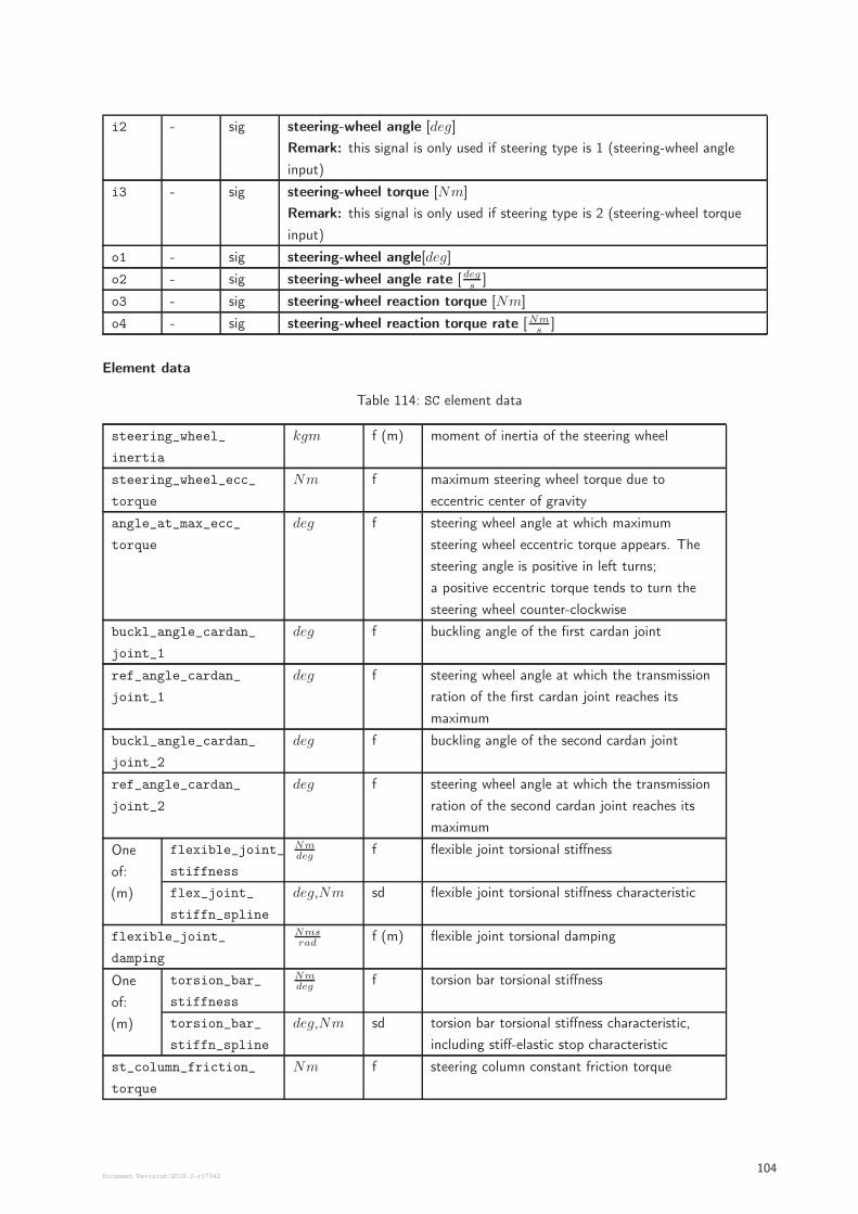
i2 - sig steering-wheel angle [deg]
Remark: this signal is only used if steering type is 1 (steering-wheel angle
input)
i3 - sig steering-wheel torque [Nm]
Remark: this signal is only used if steering type is 2 (steering-wheel torque
input)
o1 - sig steering-wheel angle[deg]
o2 - sig steering-wheel angle rate [degs
]
o3 - sig steering-wheel reaction torque [Nm]
o4 - sig steering-wheel reaction torque rate [Nms
]
Element data
Table 114: SC element data
steering_wheel_
inertia
kgm f (m) moment of inertia of the steering wheel
steering_wheel_ecc_
torque
Nm f maximum steering wheel torque due to
eccentric center of gravity
angle_at_max_ecc_
torque
deg f steering wheel angle at which maximum
steering wheel eccentric torque appears. The
steering angle is positive in left turns;
a positive eccentric torque tends to turn the
steering wheel counter-clockwise
buckl_angle_cardan_
joint_1
deg f buckling angle of the first cardan joint
ref_angle_cardan_
joint_1
deg f steering wheel angle at which the transmission
ration of the first cardan joint reaches its
maximum
buckl_angle_cardan_
joint_2
deg f buckling angle of the second cardan joint
ref_angle_cardan_
joint_2
deg f steering wheel angle at which the transmission
ration of the second cardan joint reaches its
maximum
One
of:
(m)
flexible_joint_
stiffness
Nmdeg
f flexible joint torsional stiffness
flex_joint_
stiffn_spline
deg,Nm sd flexible joint torsional stiffness characteristic
flexible_joint_
damping
Nmsrad
f (m) flexible joint torsional damping
One
of:
(m)
torsion_bar_
stiffness
Nmdeg
f torsion bar torsional stiffness
torsion_bar_
stiffn_spline
deg,Nm sd torsion bar torsional stiffness characteristic,
including stiff-elastic stop characteristic
st_column_friction_
torque
Nm f steering column constant friction torque
Document Revision:2018-2-r17342104
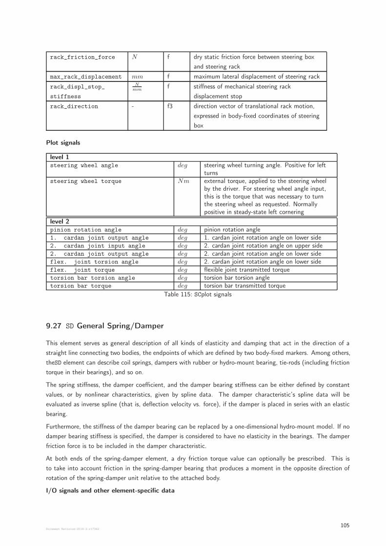
rack_friction_force N f dry static friction force between steering box
and steering rack
max_rack_displacement mm f maximum lateral displacement of steering rack
rack_displ_stop_
stiffness
Nmm
f stiffness of mechanical steering rack
displacement stop
rack_direction - f3 direction vector of translational rack motion,
expressed in body-fixed coordinates of steering
box
Plot signals
level 1steering wheel angle deg steering wheel turning angle. Positive for left
turnssteering wheel torque Nm external torque, applied to the steering wheel
by the driver. For steering wheel angle input,this is the torque that was necessary to turnthe steering wheel as requested. Normallypositive in steady-state left cornering
level 2pinion rotation angle deg pinion rotation angle1. cardan joint output angle deg 1. cardan joint rotation angle on lower side2. cardan joint input angle deg 2. cardan joint rotation angle on upper side2. cardan joint output angle deg 2. cardan joint rotation angle on lower sideflex. joint torsion angle deg 2. cardan joint rotation angle on lower sideflex. joint torque deg flexible joint transmitted torquetorsion bar torsion angle deg torsion bar torsion angletorsion bar torque deg torsion bar transmitted torque
Table 115: SCplot signals
9.27 SD General Spring/Damper
This element serves as general description of all kinds of elasticity and damping that act in the direction of a
straight line connecting two bodies, the endpoints of which are defined by two body-fixed markers. Among others,
theSD element can describe coil springs, dampers with rubber or hydro-mount bearing, tie-rods (including friction
torque in their bearings), and so on.
The spring stiffness, the damper coefficient, and the damper bearing stiffness can be either defined by constant
values, or by nonlinear characteristics, given by spline data. The damper characteristic’s spline data will be
evaluated as inverse spline (that is, deflection velocity vs. force), if the damper is placed in series with an elastic
bearing.
Furthermore, the stiffness of the damper bearing can be replaced by a one-dimensional hydro-mount model. If no
damper bearing stiffness is specified, the damper is considered to have no elasticity in the bearings. The damper
friction force is to be included in the damper characteristic.
At both ends of the spring-damper element, a dry friction torque value can optionally be prescribed. This is
to take into account friction in the spring-damper bearing that produces a moment in the opposite direction of
rotation of the spring-damper unit relative to the attached body.
I/O signals and other element-specific data
Document Revision:2018-2-r17342105
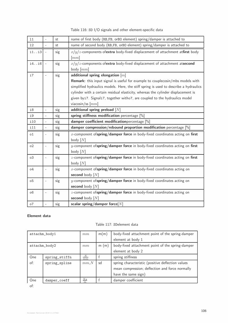
Table 116: SD I/O signals and other element-specific data
l1 - st name of first body (RB,FB, orBO element) spring/damper is attached to
l2 - st name of second body (RB,FB, orBO element) spring/damper is attached to
i1..i3 - sig x/y/z-components ofextra body-fixed displacement of attachment atfirst body
[mm]
i4..i6 - sig x/y/z-components ofextra body-fixed displacement of attachment atsecond
body [mm]
i7 - sig additional spring elongation [m]
Remark: this input signal is useful for example to couplecosin/mbs models with
simplified hydraulics models. Here, the stiff spring is used to describe a hydraulics
cylinder with a certain residual elasticity, whereas the cylinder displacement is
given byi7. Signali7, together witho7, are coupled to the hydraulics model
viacosin/ss [mm]
i8 - sig additional spring preload [N ]
i9 - sig spring stiffness modification percentage [%]
i10 - sig damper coefficient modificationpercentage [%]
i11 - sig damper compression/rebound proportion modification percentage [%]
o1 - sig x-component ofspring/damper force in body-fixed coordinates acting on first
body [N ]
o2 - sig y-component ofspring/damper force in body-fixed coordinates acting on first
body [N ]
o3 - sig z-component ofspring/damper force in body-fixed coordinates acting on first
body [N ]
o4 - sig x-component ofspring/damper force in body-fixed coordinates acting on
second body [N ]
o5 - sig y-component ofspring/damper force in body-fixed coordinates acting on
second body [N ]
o6 - sig z-component ofspring/damper force in body-fixed coordinates acting on
second body [N ]
o7 - sig scalar spring/damper force[N ]
Element data
Table 117: SDelement data
attachm_body1 mm m(m) body-fixed attachment point of the spring-damper
element at body 1
attachm_body2 mm m (m) body-fixed attachment point of the spring-damper
element at body 2
One
of:
spring_stiffn Nmm
f spring stiffness
spring_spline mm,N sd spring characteristic (positive deflection values
mean compression; deflection and force normally
have the same sign)
One
of:
damper_coeff Nsm
f damper coefficient
Document Revision:2018-2-r17342106
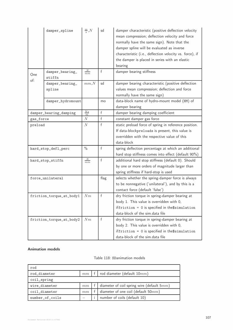
damper_spline ms,N sd damper characteristic (positive deflection velocity
mean compression; deflection velocity and force
normally have the same sign). Note that the
damper spline will be evaluated as inverse
characteristic (i.e., deflection velocity vs. force), if
the damper is placed in series with an elastic
bearing
One
of:
damper_bearing_
stiffn
Nmm
f damper bearing stiffness
damper_bearing_
spline
mm,N sd damper bearing characteristic (positive deflection
values mean compression; deflection and force
normally have the same sign)
damper_hydromount mo data-block name of hydro-mount model (HM) of
damper bearing
damper_bearing_damping Nsm
f damper bearing damping coefficient
gas_force N f constant damper gas force
preload N f static preload force of spring in reference position.
If data-blockpreloads is present, this value is
overridden with the respective value of this
data-block
hard_stop_defl_perc % f spring deflection percentage at which an additional
hard stop stiffness comes into effect (default 90%)
hard_stop_stiffn Nmm
f additional hard stop stiffness (default 0). Should
by one or more orders of magnitude larger than
spring stiffness if hard-stop is used
force_unilateral flag selects whether the spring-damper force is always
to be nonnegative (‘unilateral’), and by this is a
contact force (default ‘false’)
friction_torque_at_body1 Nm f dry friction torque in spring-damper bearing at
body 1. This value is overridden with 0,
iffriction = 0 is specified in the$simulation
data-block of the sim.data file
friction_torque_at_body2 Nm f dry friction torque in spring-damper bearing at
body 2. This value is overridden with 0,
iffriction = 0 is specified in the$simulation
data-block of the sim.data file
Animation models
Table 118: SDanimation models
rod
rod_diameter mm f rod diameter (default 10mm)
coil_spring
wire_diameter mm f diameter of coil spring wire (default 5mm)
coil_diameter mm f diameter of one coil (default 50mm)
number_of_coils − i number of coils (default 10)
Document Revision:2018-2-r17342107
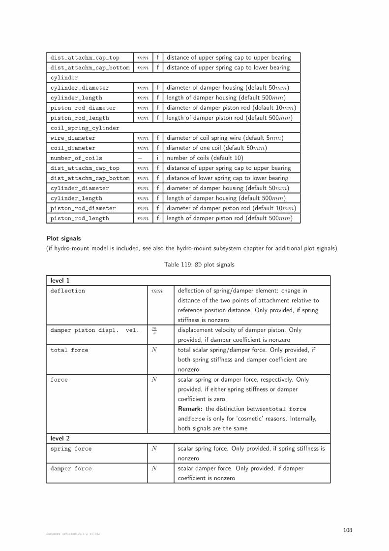
dist_attachm_cap_top mm f distance of upper spring cap to upper bearing
dist_attachm_cap_bottom mm f distance of upper spring cap to lower bearing
cylinder
cylinder_diameter mm f diameter of damper housing (default 50mm)
cylinder_length mm f length of damper housing (default 500mm)
piston_rod_diameter mm f diameter of damper piston rod (default 10mm)
piston_rod_length mm f length of damper piston rod (default 500mm)
coil_spring_cylinder
wire_diameter mm f diameter of coil spring wire (default 5mm)
coil_diameter mm f diameter of one coil (default 50mm)
number_of_coils − i number of coils (default 10)
dist_attachm_cap_top mm f distance of upper spring cap to upper bearing
dist_attachm_cap_bottom mm f distance of lower spring cap to lower bearing
cylinder_diameter mm f diameter of damper housing (default 50mm)
cylinder_length mm f length of damper housing (default 500mm)
piston_rod_diameter mm f diameter of damper piston rod (default 10mm)
piston_rod_length mm f length of damper piston rod (default 500mm)
Plot signals
(if hydro-mount model is included, see also the hydro-mount subsystem chapter for additional plot signals)
Table 119: SD plot signals
level 1
deflection mm deflection of spring/damper element: change in
distance of the two points of attachment relative to
reference position distance. Only provided, if spring
stiffness is nonzero
damper piston displ. vel. ms
displacement velocity of damper piston. Only
provided, if damper coefficient is nonzero
total force N total scalar spring/damper force. Only provided, if
both spring stiffness and damper coefficient are
nonzero
force N scalar spring or damper force, respectively. Only
provided, if either spring stiffness or damper
coefficient is zero.
Remark: the distinction betweentotal force
andforce is only for ‘cosmetic’ reasons. Internally,
both signals are the same
level 2
spring force N scalar spring force. Only provided, if spring stiffness is
nonzero
damper force N scalar damper force. Only provided, if damper
coefficient is nonzero
Document Revision:2018-2-r17342108
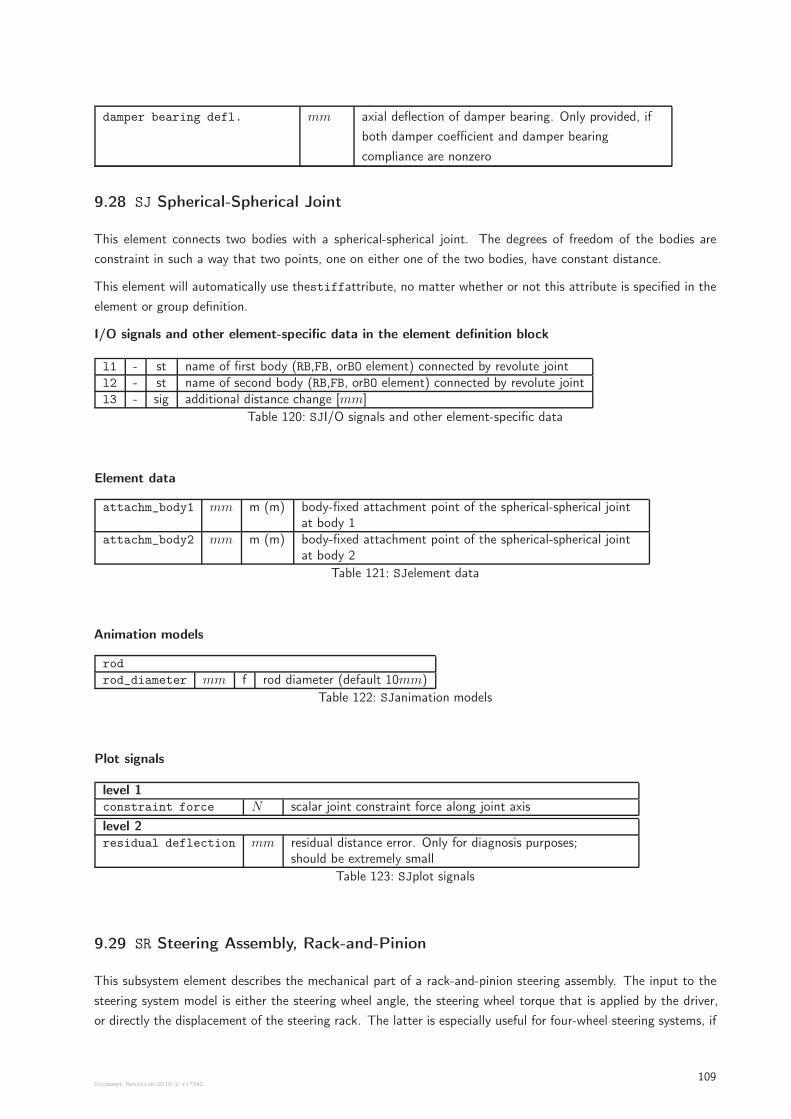
damper bearing defl. mm axial deflection of damper bearing. Only provided, if
both damper coefficient and damper bearing
compliance are nonzero
9.28 SJ Spherical-Spherical Joint
This element connects two bodies with a spherical-spherical joint. The degrees of freedom of the bodies are
constraint in such a way that two points, one on either one of the two bodies, have constant distance.
This element will automatically use thestiffattribute, no matter whether or not this attribute is specified in the
element or group definition.
I/O signals and other element-specific data in the element definition block
l1 - st name of first body (RB,FB, orBO element) connected by revolute jointl2 - st name of second body (RB,FB, orBO element) connected by revolute jointl3 - sig additional distance change [mm]
Table 120: SJI/O signals and other element-specific data
Element data
attachm_body1 mm m (m) body-fixed attachment point of the spherical-spherical jointat body 1
attachm_body2 mm m (m) body-fixed attachment point of the spherical-spherical jointat body 2
Table 121: SJelement data
Animation models
rod
rod_diameter mm f rod diameter (default 10mm)
Table 122: SJanimation models
Plot signals
level 1constraint force N scalar joint constraint force along joint axis
level 2residual deflection mm residual distance error. Only for diagnosis purposes;
should be extremely small
Table 123: SJplot signals
9.29 SR Steering Assembly, Rack-and-Pinion
This subsystem element describes the mechanical part of a rack-and-pinion steering assembly. The input to the
steering system model is either the steering wheel angle, the steering wheel torque that is applied by the driver,
or directly the displacement of the steering rack. The latter is especially useful for four-wheel steering systems, if
Document Revision:2018-2-r17342109
the rack displacement of the rear steering-box is controlled by wire. During a simulation, you may switch between
the different input types.
At present, no dynamic hydraulic power-steering model is implemented yet, but only a steady-state torque/force
amplification characteristic. A more detailed hydraulic power-steering model will be added in a future release
ofcosin/mbs.
The steering model comprises
• a steering wheel with moment of inertia and eccentric center of gravity
• a steering column with
– two cardan joints, defined by prescribed buckling angles and respective reference angles that describe
the angular position of maximum transmission ratio
– a flexible joint between the cardan joints, including damping
– dry friction torque
• a torsion bar stiffness and damping, the torque of which serves as input to the power-steering characteristic
• a rack-and-pinion contact stiffness, damping, and play
• a steering gear-box with
– constant or variable transmission ratio
– stiff-elastic steering-rack stop
• a steering damper, located between rack and steering gear-box
• a dry friction element, located between rack and steering gear-box
• an optional quasi-static hydraulic power steering model
• an optional dynamic electric power steering (EPS) model.
Both flexible joint stiffness and torsion bar stiffness can optionally be described nonlinearly, using spline data.
The steering model can be viewed to be a (very sophisticated) force element, acting between the steering box
(which might be fixed to car-body, or modeled as a free mass), and the steering rack. This general force consists
of a constraint force that is defining a translational joint between steering box and steering rack, a friction force,
a highly nonlinear spring force describing a mechanical stop, and the contact force between rack and pinion. The
latter itself is a result of the steering column model, outlined above.
It is recommended to use thestiffattribute for this element, due to the constraint forces that are modeled as
extremely stiff elasticities.
Typically, the steering model will be completed by two rigid bodies: steering box and steering rack. The latter
will typically be connected to the front or rear wheel-carriers by two very stiff spring-damper elements, describing
the tie-rods.
The mechanical steering model is completed with interfaces to several ECU’s:
• four-wheel steering (4WS) ECU, controlling the rack displacement of a rear axle steering
• standard EPS (Electronic Power Steering), providing an additional torque acting on the steering column, as
well as an additional force acting on the steering rack
• advanced EPS, using several additional input signals as compared to standard EPS.
Document Revision:2018-2-r17342110
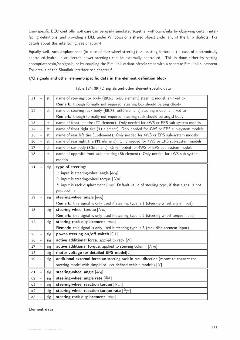
User-specific ECU controller software can be easily simulated together withcosin/mbs by observing certain inter-
facing definitions, and providing a DLL under Windows or a shared object under any of the Unix dialects. For
details about this interfacing, see chapter 4.
Equally well, rack displacement (in case of four-wheel steering) or assisting fortorque (in case of electronically
controlled hydraulic or electric power steering) can be externally controlled. This is done either by setting
appropriatecosin/ss signals, or by coupling the Simulink variant ofcosin/mbs with a separate Simulink subsystem.
For details of the Simulink interface see chapter 6.
I/O signals and other element-specific data in the element definition block
Table 124: SRI/O signals and other element-specific data
l1 - st name of steering box body (RB,FB, orBO element) steering model is linked to
Remark: though formally not required, steering box should be arigidbody
l2 - st name of steering rack body (RB,FB, orBO element) steering model is linked to
Remark: though formally not required, steering rack should be arigid body
l3 - st name of front left tire (TI element). Only needed for 4WS or EPS sub-system models
l4 - st name of front right tire (TI element). Only needed for 4WS or EPS sub-system models
l5 - st name of rear left tire (TIelement). Only needed for 4WS or EPS sub-system models
l6 - st name of rear right tire (TI element). Only needed for 4WS or EPS sub-system models
l7 - st name of car-body (BOelement). Only needed for 4WS or EPS sub-system models
l8 - st name of opposite front axle steering (SR element). Only needed for 4WS sub-system
models
i1 - sig type of steering:
1: input is steering-wheel angle [deg]
2: input is steering-wheel torque [Nm]
3: input is rack displacement [mm] Default value of steering type, if that signal is not
provided: 1
i2 - sig steering-wheel angle [deg]
Remark: this signal is only used if steering type is 1 (steering-wheel angle input)
i3 - sig steering-wheel torque [Nm]
Remark: this signal is only used if steering type is 2 (steering-wheel torque input)
i4 - sig steering-rack displacement [mm]
Remark: this signal is only used if steering type is 3 (rack displacement input)
i5 - sig power-steering on/off switch [0,1]
i6 - sig active additional force, applied to rack [N ]
i7 - sig active additional torque, applied to steering column [Nm]
i8 - sig motor voltage for detailed EPS model[V ]
i9 - sig additional external force on steering rack in rack direction (meant to connect the
steering model with simplified user-defined vehicle models) [N ]
o1 - sig steering-wheel angle [deg]
o2 - sig steering-wheel angle rate [degs
]
o3 - sig steering-wheel reaction torque [Nm]
o4 - sig steering-wheel reaction torque rate [Nms
]
o5 - sig steering rack displacement [mm]
Element data
Document Revision:2018-2-r17342111
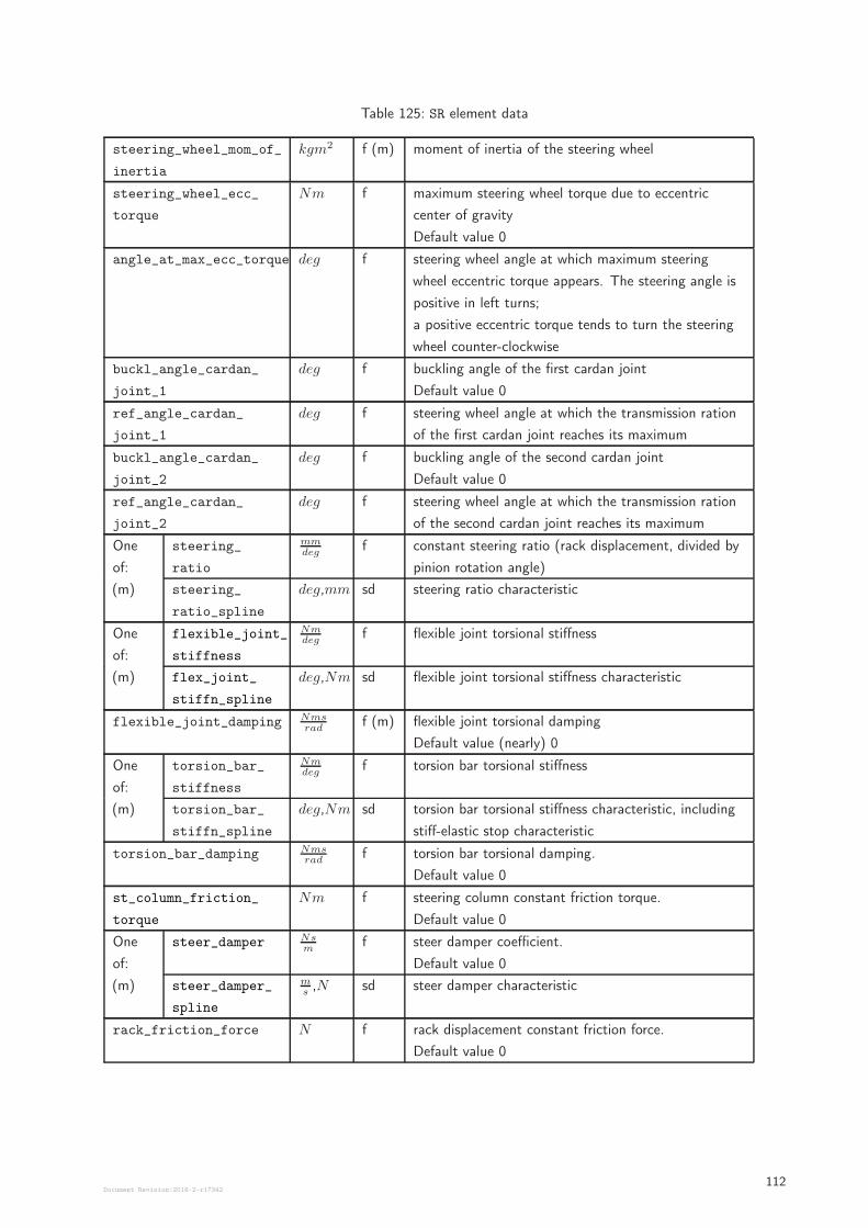
Table 125: SR element data
steering_wheel_mom_of_
inertia
kgm2 f (m) moment of inertia of the steering wheel
steering_wheel_ecc_
torque
Nm f maximum steering wheel torque due to eccentric
center of gravity
Default value 0
angle_at_max_ecc_torque deg f steering wheel angle at which maximum steering
wheel eccentric torque appears. The steering angle is
positive in left turns;
a positive eccentric torque tends to turn the steering
wheel counter-clockwise
buckl_angle_cardan_
joint_1
deg f buckling angle of the first cardan joint
Default value 0
ref_angle_cardan_
joint_1
deg f steering wheel angle at which the transmission ration
of the first cardan joint reaches its maximum
buckl_angle_cardan_
joint_2
deg f buckling angle of the second cardan joint
Default value 0
ref_angle_cardan_
joint_2
deg f steering wheel angle at which the transmission ration
of the second cardan joint reaches its maximum
One
of:
(m)
steering_
ratio
mmdeg
f constant steering ratio (rack displacement, divided by
pinion rotation angle)
steering_
ratio_spline
deg,mm sd steering ratio characteristic
One
of:
(m)
flexible_joint_
stiffness
Nmdeg
f flexible joint torsional stiffness
flex_joint_
stiffn_spline
deg,Nm sd flexible joint torsional stiffness characteristic
flexible_joint_damping Nmsrad
f (m) flexible joint torsional damping
Default value (nearly) 0
One
of:
(m)
torsion_bar_
stiffness
Nmdeg
f torsion bar torsional stiffness
torsion_bar_
stiffn_spline
deg,Nm sd torsion bar torsional stiffness characteristic, including
stiff-elastic stop characteristic
torsion_bar_damping Nmsrad
f torsion bar torsional damping.
Default value 0
st_column_friction_
torque
Nm f steering column constant friction torque.
Default value 0
One
of:
(m)
steer_damper Nsm
f steer damper coefficient.
Default value 0
steer_damper_
spline
ms,N sd steer damper characteristic
rack_friction_force N f rack displacement constant friction force.
Default value 0
Document Revision:2018-2-r17342112
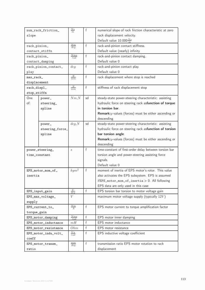
num_rack_friction_
slope
Nsm
f numerical slope of rack friction characteristic at zero
rack displacement velocity.
Default value 10.000Nsm
rack_pinion_
contact_stiffn
Nmdeg
f rack-and-pinion contact stiffness.
Default value (nearly) infinity
rack_pinion_
contact_damping
Nmsrad
f rack-and-pinion contact damping.
Default value 0
rack_pinion_contact_
play
deg f rack-and-pinion contact play.
Default value 0
max_rack_
displacement
Nmm
f rack displacement where stop is reached
rack_displ_
stop_stiffn
Nmm
f stiffness of rack displacement stop
One
of:
power_
steering_
spline
Nm,N sd steady-state power-steering characteristic: assisting
hydraulic force on steering rack asfunction of torque
in torsion bar.
Remark:y-values (forces) must be either ascending or
descending
power_
steering_force_
spline
deg,N sd steady-state power-steering characteristic: assisting
hydraulic force on steering rack asfunction of torsion
bar torsion angle.
Remark:y-values (forces) must be either ascending or
descending
power_steering_
time_constant
s f time-constant of first-order delay between torsion bar
torsion angle and power-steering assisting force
signals.
Default value 0
EPS_motor_mom_of_
inertia
kgm2 f moment of inertia of EPS motor’s rotor. This value
also activates the EPS subsystem. EPS is assumed
ifEPS_motor_mom_of_inertia > 0. All following
EPS data are only used in this case
EPS_input_gain Vdeg
f EPS torsion bar torsion to motor voltage gain
EPS_max_voltage_
supply
V maximum motor voltage supply (typically 12V )
EPS_current_to_
torque_gain
NmA
f EPS motor current to torque amplification factor
EPS_motor_damping Nmsrad
f EPS motor inner damping
EPS_motor_inductance mH f EPS motor inductance
EPS_motor_resistance Ohm f EPS motor resistance
EPS_motor_indu_volt_
coeff
V srad
f EPS inductive voltage coefficient
EPS_motor_transm_
ratio
mmdeg
f transmission ratio EPS motor rotation to rack
displacement
Document Revision:2018-2-r17342113
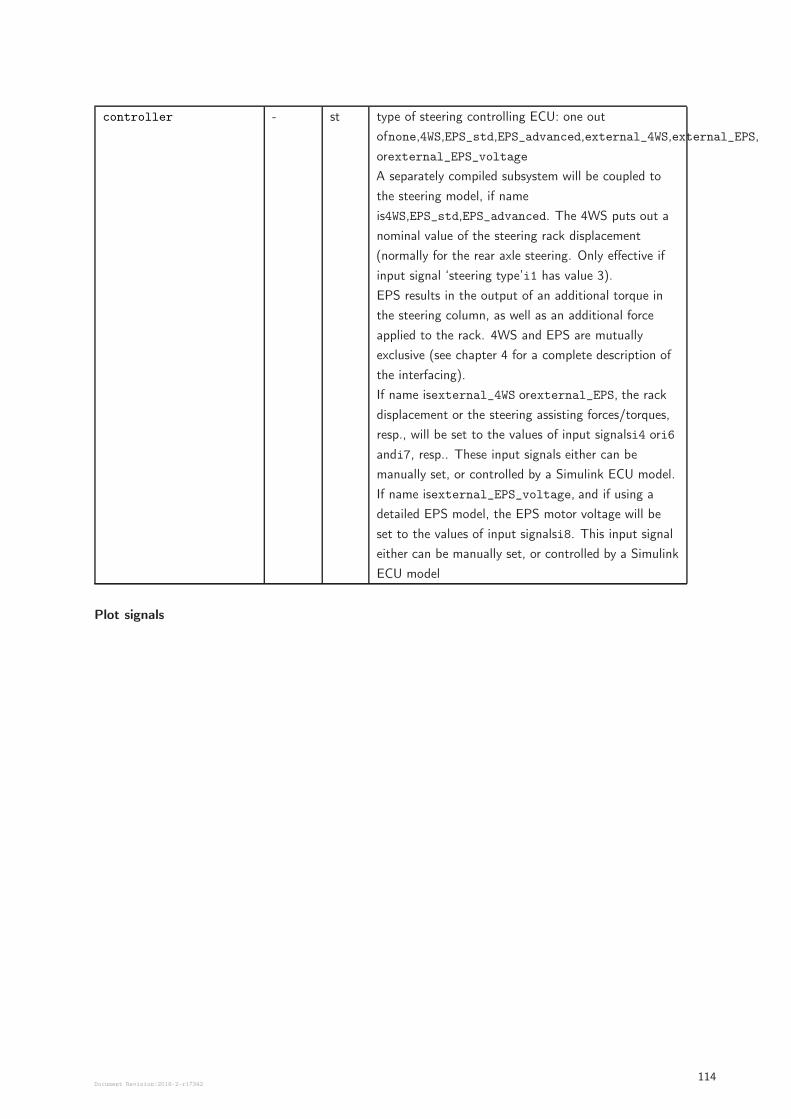
controller - st type of steering controlling ECU: one out
ofnone,4WS,EPS_std,EPS_advanced,external_4WS,external_EPS,
orexternal_EPS_voltage
A separately compiled subsystem will be coupled to
the steering model, if name
is4WS,EPS_std,EPS_advanced. The 4WS puts out a
nominal value of the steering rack displacement
(normally for the rear axle steering. Only effective if
input signal ‘steering type’i1 has value 3).
EPS results in the output of an additional torque in
the steering column, as well as an additional force
applied to the rack. 4WS and EPS are mutually
exclusive (see chapter 4 for a complete description of
the interfacing).
If name isexternal_4WS orexternal_EPS, the rack
displacement or the steering assisting forces/torques,
resp., will be set to the values of input signalsi4 ori6
andi7, resp.. These input signals either can be
manually set, or controlled by a Simulink ECU model.
If name isexternal_EPS_voltage, and if using a
detailed EPS model, the EPS motor voltage will be
set to the values of input signalsi8. This input signal
either can be manually set, or controlled by a Simulink
ECU model
Plot signals
Document Revision:2018-2-r17342114
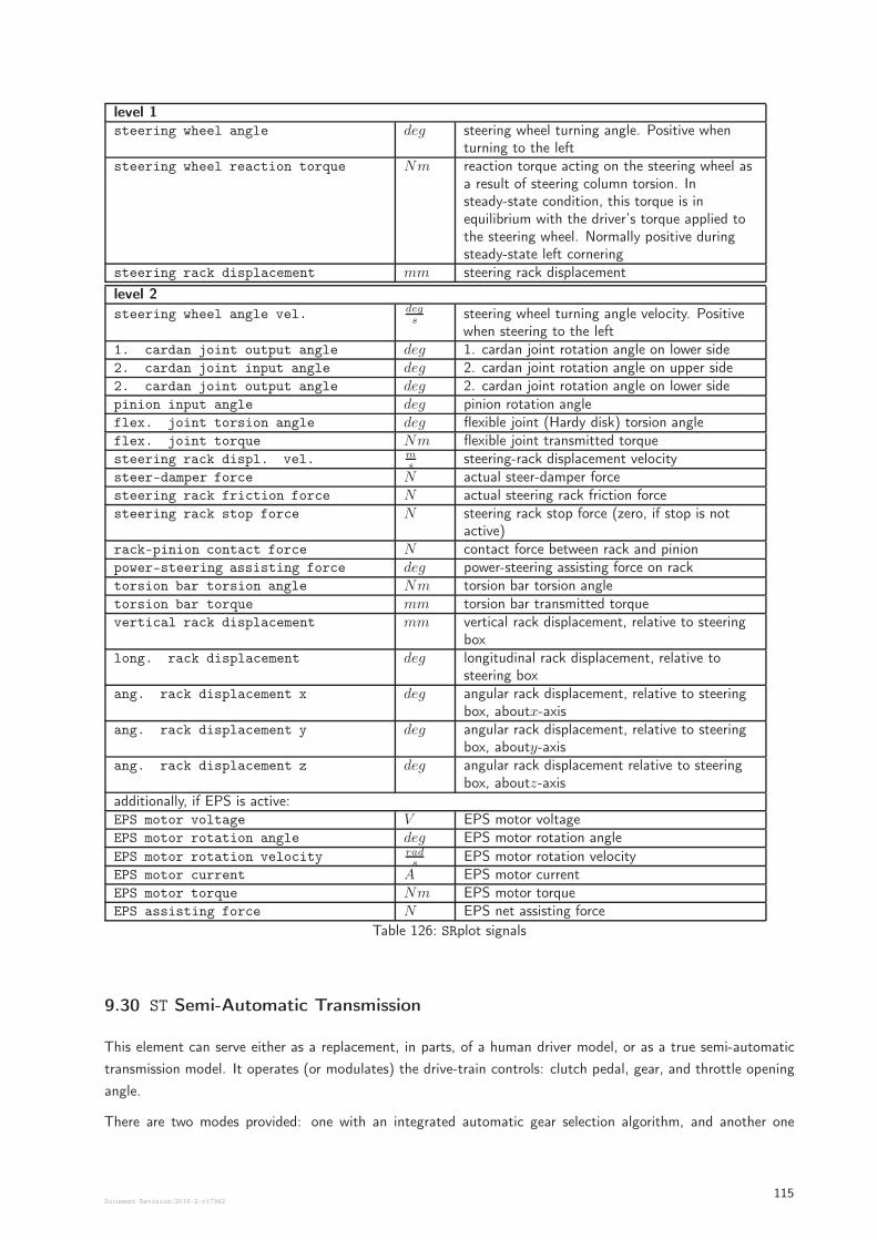
level 1steering wheel angle deg steering wheel turning angle. Positive when
turning to the leftsteering wheel reaction torque Nm reaction torque acting on the steering wheel as
a result of steering column torsion. Insteady-state condition, this torque is inequilibrium with the driver’s torque applied tothe steering wheel. Normally positive duringsteady-state left cornering
steering rack displacement mm steering rack displacement
level 2
steering wheel angle vel. degs
steering wheel turning angle velocity. Positivewhen steering to the left
1. cardan joint output angle deg 1. cardan joint rotation angle on lower side2. cardan joint input angle deg 2. cardan joint rotation angle on upper side2. cardan joint output angle deg 2. cardan joint rotation angle on lower sidepinion input angle deg pinion rotation angleflex. joint torsion angle deg flexible joint (Hardy disk) torsion angleflex. joint torque Nm flexible joint transmitted torquesteering rack displ. vel. m
ssteering-rack displacement velocity
steer-damper force N actual steer-damper forcesteering rack friction force N actual steering rack friction forcesteering rack stop force N steering rack stop force (zero, if stop is not
active)rack-pinion contact force N contact force between rack and pinionpower-steering assisting force deg power-steering assisting force on racktorsion bar torsion angle Nm torsion bar torsion angletorsion bar torque mm torsion bar transmitted torquevertical rack displacement mm vertical rack displacement, relative to steering
boxlong. rack displacement deg longitudinal rack displacement, relative to
steering boxang. rack displacement x deg angular rack displacement, relative to steering
box, aboutx-axisang. rack displacement y deg angular rack displacement, relative to steering
box, abouty-axisang. rack displacement z deg angular rack displacement relative to steering
box, aboutz-axisadditionally, if EPS is active:EPS motor voltage V EPS motor voltageEPS motor rotation angle deg EPS motor rotation angle
EPS motor rotation velocity rads
EPS motor rotation velocityEPS motor current A EPS motor currentEPS motor torque Nm EPS motor torqueEPS assisting force N EPS net assisting force
Table 126: SRplot signals
9.30 ST Semi-Automatic Transmission
This element can serve either as a replacement, in parts, of a human driver model, or as a true semi-automatic
transmission model. It operates (or modulates) the drive-train controls: clutch pedal, gear, and throttle opening
angle.
There are two modes provided: one with an integrated automatic gear selection algorithm, and another one
Document Revision:2018-2-r17342115
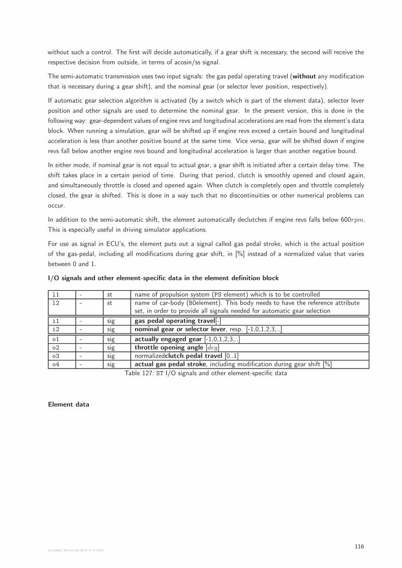
without such a control. The first will decide automatically, if a gear shift is necessary, the second will receive the
respective decision from outside, in terms of acosin/ss signal.
The semi-automatic transmission uses two input signals: the gas pedal operating travel (without any modification
that is necessary during a gear shift), and the nominal gear (or selector lever position, respectively).
If automatic gear selection algorithm is activated (by a switch which is part of the element data), selector lever
position and other signals are used to determine the nominal gear. In the present version, this is done in the
following way: gear-dependent values of engine revs and longitudinal accelerations are read from the element’s data
block. When running a simulation, gear will be shifted up if engine revs exceed a certain bound and longitudinal
acceleration is less than another positive bound at the same time. Vice versa, gear will be shifted down if engine
revs fall below another engine revs bound and longitudinal acceleration is larger than another negative bound.
In either mode, if nominal gear is not equal to actual gear, a gear shift is initiated after a certain delay time. The
shift takes place in a certain period of time. During that period, clutch is smoothly opened and closed again,
and simultaneously throttle is closed and opened again. When clutch is completely open and throttle completely
closed, the gear is shifted. This is done in a way such that no discontinuities or other numerical problems can
occur.
In addition to the semi-automatic shift, the element automatically declutches if engine revs falls below 600rpm.
This is especially useful in driving simulator applications.
For use as signal in ECU’s, the element puts out a signal called gas pedal stroke, which is the actual position
of the gas-pedal, including all modifications during gear shift, in [%] instead of a normalized value that varies
between 0 and 1.
I/O signals and other element-specific data in the element definition block
l1 - st name of propulsion system (PS element) which is to be controlledl2 - st name of car-body (BOelement). This body needs to have the reference attribute
set, in order to provide all signals needed for automatic gear selection
i1 - sig gas pedal operating travel[-]i2 - sig nominal gear or selector lever, resp. [-1,0,1,2,3,..]
o1 - sig actually engaged gear [-1,0,1,2,3,..]o2 - sig throttle opening angle [deg]o3 - sig normalizedclutch pedal travel [0..1]o4 - sig actual gas pedal stroke, including modification during gear shift [%]
Table 127: ST I/O signals and other element-specific data
Element data
Document Revision:2018-2-r17342116
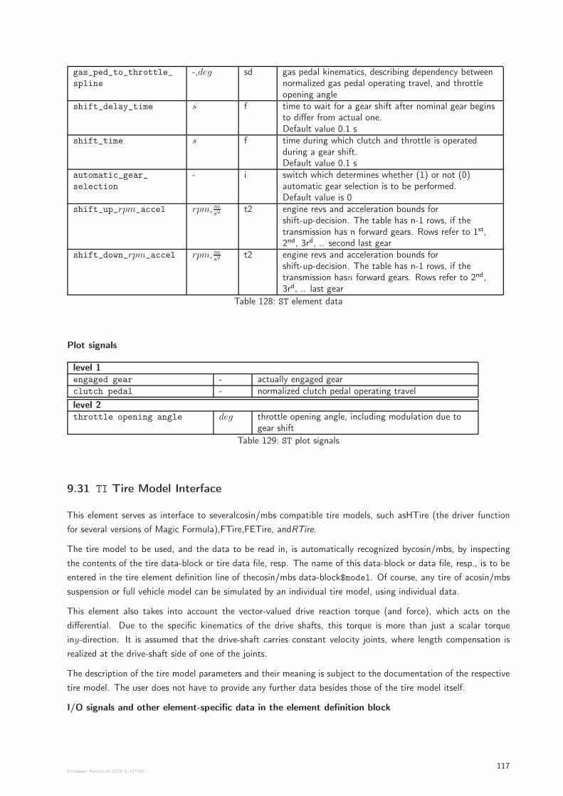
gas_ped_to_throttle_
spline
-,deg sd gas pedal kinematics, describing dependency betweennormalized gas pedal operating travel, and throttleopening angle
shift_delay_time s f time to wait for a gear shift after nominal gear beginsto differ from actual one.Default value 0.1 s
shift_time s f time during which clutch and throttle is operatedduring a gear shift.Default value 0.1 s
automatic_gear_
selection
- i switch which determines whether (1) or not (0)automatic gear selection is to be performed.Default value is 0
shift_up_rpm_accel rpm,ms2
t2 engine revs and acceleration bounds forshift-up-decision. The table has n-1 rows, if thetransmission has n forward gears. Rows refer to 1st,2nd, 3rd, .. second last gear
shift_down_rpm_accel rpm,ms2
t2 engine revs and acceleration bounds forshift-up-decision. The table has n-1 rows, if thetransmission hasn forward gears. Rows refer to 2nd,3rd, .. last gear
Table 128: ST element data
Plot signals
level 1engaged gear - actually engaged gearclutch pedal - normalized clutch pedal operating travel
level 2throttle opening angle deg throttle opening angle, including modulation due to
gear shift
Table 129: ST plot signals
9.31 TI Tire Model Interface
This element serves as interface to severalcosin/mbs compatible tire models, such asHTire (the driver function
for several versions of Magic Formula),FTire,FETire, andRTire.
The tire model to be used, and the data to be read in, is automatically recognized bycosin/mbs, by inspecting
the contents of the tire data-block or tire data file, resp. The name of this data-block or data file, resp., is to be
entered in the tire element definition line of thecosin/mbs data-block$model. Of course, any tire of acosin/mbs
suspension or full vehicle model can be simulated by an individual tire model, using individual data.
This element also takes into account the vector-valued drive reaction torque (and force), which acts on the
differential. Due to the specific kinematics of the drive shafts, this torque is more than just a scalar torque
iny-direction. It is assumed that the drive-shaft carries constant velocity joints, where length compensation is
realized at the drive-shaft side of one of the joints.
The description of the tire model parameters and their meaning is subject to the documentation of the respective
tire model. The user does not have to provide any further data besides those of the tire model itself.
I/O signals and other element-specific data in the element definition block
Document Revision:2018-2-r17342117
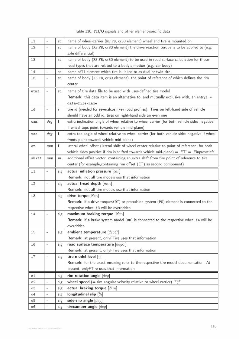
Table 130: TII/O signals and other element-specific data
l1 - st name of wheel-carrier (RB,FB, orBO element) wheel and tire is mounted on
l2 - st name of body (RB,FB, orBO element) the drive reaction torque is to be applied to (e.g.
axle differential)
l3 - st name of body (RB,FB, orBO element) to be used in road surface calculation for those
road types that are related to a body’s motion (e.g. car-body)
l4 - st name ofTI element which tire is linked to as dual or twin tire
l5 - st name of body (RB,FB, orBO element), the point of reference of which defines the rim
center
utmf - st name of tire data file to be used with user-defined tire model
Remark: this data item is an alternative to, and mutually exclusive with, an entryf =
data-file-name
id - i tire id (needed for severalcosin/ev road profiles). Tires on left-hand side of vehicle
should have an odd id, tires on right-hand side an even one
cam deg f extra inclination angle of wheel relative to wheel carrier (for both vehicle sides negative
if wheel tops point towards vehicle mid-plane)
toe deg f extra toe angle of wheel relative to wheel carrier (for both vehicle sides negative if wheel
fronts point towards vehicle mid-plane)
et mm f lateral wheel offset (lateral shift of wheel center relative to point of reference; for both
vehicle sides positive if rim is shifted towards vehicle mid-plane) = ’ET’ = ’Einpresstiefe’
shift mm m additional offset vector, containing an extra shift from tire point of reference to tire
center (for example,containing rim offset (ET) as second component)
i1 - sig actual inflation pressure [bar]
Remark: not all tire models use that information
i2 - sig actual tread depth [mm]
Remark: not all tire models use that information
i3 - sig drive torque[Nm]
Remark: if a drive torques(DT) or propulsion system (PS) element is connected to the
respective wheel,i3 will be overridden
i4 - sig maximum braking torque [Nm]
Remark: if a brake system model (BR) is connected to the respective wheel,i4 will be
overridden
i5 - sig ambient temperature [degC]
Remark: at present, onlyFTire uses that information
i6 - sig road surface temperature [degC]
Remark: at present, onlyFTire uses that information
i7 - sig tire model level [-]
Remark: for the exact meaning refer to the respective tire model documentation. At
present, onlyFTire uses that information
o1 - sig rim rotation angle [deg]
o2 - sig wheel speed (= rim angular velocity relative to wheel carrier) [ rads
]
o3 - sig actual braking torque [Nm]
o4 - sig longitudinal slip [%]
o5 - sig side-slip angle [deg]
o6 - sig tirecamber angle [deg]
Document Revision:2018-2-r17342118
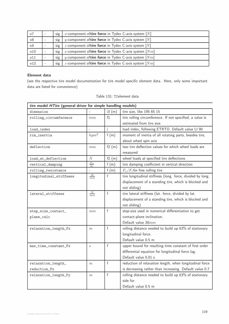
o7 - sig x-component oftire force in Tydex C-axis system [N ]
o8 - sig y-component oftire force in Tydex C-axis system [N ]
o9 - sig z-component oftire force in Tydex C-axis system [N ]
o10 - sig x-component oftire force in Tydex C-axis system [Nm]
o11 - sig y-component oftire force in Tydex C-axis system [Nm]
o12 - sig z-component oftire force in Tydex C-axis system [Nm]
Element data
(see the respective tire model documentation for tire model specific element data. Here, only some important
data are listed for convenience)
Table 131: TIelement data
tire model HTire (general driver for simple handling models)
dimension - i3 (m) tire size, like 195 65 15
rolling_circumference mm f1 tire rolling circumference. If not specified, a value is
estimated from tire size
load_index - i load index, following ETRTO. Default value LI 90
rim_inertia kgm2 f (m) moment of inertia of all rotating parts, besides tire,
about wheel spin axis
deflection mm f2 (m) two tire deflection values for which wheel loads are
measured
load_at_deflection N f2 (m) wheel loads at specified tire deflections
vertical_damping Nsm
f (m) tire damping coefficient in vertical direction
rolling_resistance - f (m) Fx/Fzfor free rolling tire
longitudinal_stiffness Nmm
f tire longitudinal stiffness (long. force, divided by long.
displacement of a standing tire, which is blocked and
not sliding)
lateral_stiffness Nmm
f tire lateral stiffness (lat. force, divided by lat.
displacement of a standing tire, which is blocked and
not sliding)
step_size_contact_
plane_calc
mm f step-size used in numerical differentiation to get
contact-plane inclination.
Default value 30mm
relaxation_length_Fx m f rolling distance needed to build up 63% of stationary
longitudinal force.
Default value 0.5 m
max_time_constant_Fx s f upper bound for resulting time constant of first order
differential equation for longitudinal force lag.
Default value 0.01 s
relaxation_length_
reduction_Fx
m f reduction of relaxation length, when longitudinal force
is decreasing rather than increasing. Default value 0.7
relaxation_length_Fy m f rolling distance needed to build up 63% of stationary
side for.
Default value 0.5 m
Document Revision:2018-2-r17342119
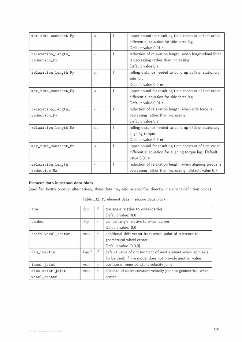
max_time_constant_Fy s f upper bound for resulting time constant of first order
differential equation for side force lag.
Default value 0.01 s
relaxation_length_
reduction_Fx
- f reduction of relaxation length, when longitudinal force
is decreasing rather than increasing.
Default value 0.7
relaxation_length_Fy m f rolling distance needed to build up 63% of stationary
side for.
Default value 0.5 m
max_time_constant_Fy s f upper bound for resulting time constant of first order
differential equation for side force lag.
Default value 0.01 s
relaxation_length_
reduction_Fy
- f reduction of relaxation length, when side force is
decreasing rather than increasing.
Default value 0.7
relaxation_length_Mz m f rolling distance needed to build up 63% of stationary
aligning torque.
Default value 0.5 m
max_time_constant_Mz s f upper bound for resulting time constant of first order
differential equation for aligning torque lag. Default
value 0.01 s
relaxation_length_
reduction_Mz
- f reduction of relaxation length, when aligning torque is
decreasing rather than increasing. Default value 0.7
Element data in second data block
(specified bydb2 ormdb2; alternatively, these data may also be specified directly in element definition block)
Table 132: TI element data in second data block
toe deg f toe angle relative to wheel-carrier.
Default value: 0.0
camber deg f camber angle relative to wheel-carrier.
Default value: 0.0
shift_wheel_center mm f additional shift vector from wheel point of reference to
geometrical wheel center.
Default value [0,0,0]
rim_inertia kgm2 f default value of rim moment of inertia about wheel spin axis.
To be used, if tire model does not provide another value
inner_joint mm m position of inner constant velocity joint
dist_outer_joint_
wheel_center
mm f distance of outer constant velocity joint to geometrical wheel
center
Document Revision:2018-2-r17342120
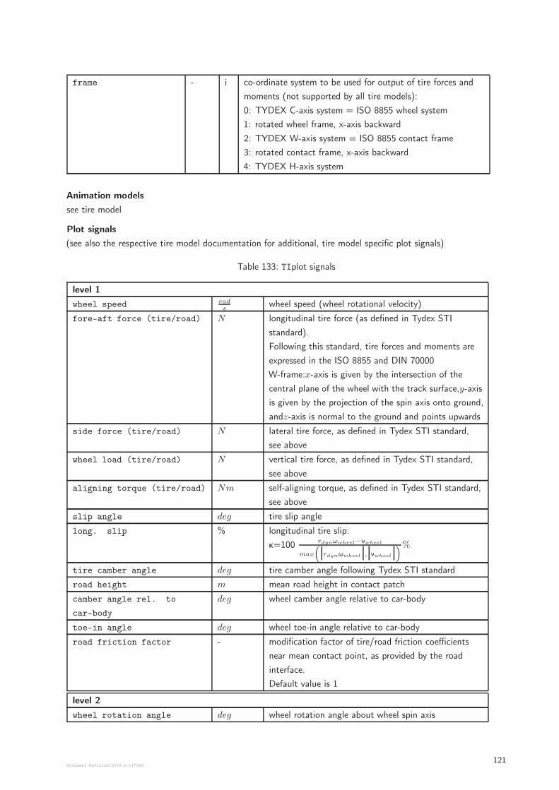
frame - i co-ordinate system to be used for output of tire forces and
moments (not supported by all tire models):
0: TYDEX C-axis system = ISO 8855 wheel system
1: rotated wheel frame, x-axis backward
2: TYDEX W-axis system = ISO 8855 contact frame
3: rotated contact frame, x-axis backward
4: TYDEX H-axis system
Animation models
see tire model
Plot signals
(see also the respective tire model documentation for additional, tire model specific plot signals)
Table 133: TIplot signals
level 1
wheel speed rads
wheel speed (wheel rotational velocity)
fore-aft force (tire/road) N longitudinal tire force (as defined in Tydex STI
standard).
Following this standard, tire forces and moments are
expressed in the ISO 8855 and DIN 70000
W-frame:x-axis is given by the intersection of the
central plane of the wheel with the track surface,y-axis
is given by the projection of the spin axis onto ground,
andz-axis is normal to the ground and points upwards
side force (tire/road) N lateral tire force, as defined in Tydex STI standard,
see above
wheel load (tire/road) N vertical tire force, as defined in Tydex STI standard,
see above
aligning torque (tire/road) Nm self-aligning torque, as defined in Tydex STI standard,
see above
slip angle deg tire slip angle
long. slip % longitudinal tire slip:
κ=100rdynωwheel−νwheel
max
(
rdynωwheel , νwheel
)%
tire camber angle deg tire camber angle following Tydex STI standard
road height m mean road height in contact patch
camber angle rel. to
car-body
deg wheel camber angle relative to car-body
toe-in angle deg wheel toe-in angle relative to car-body
road friction factor - modification factor of tire/road friction coefficients
near mean contact point, as provided by the road
interface.
Default value is 1
level 2
wheel rotation angle deg wheel rotation angle about wheel spin axis
Document Revision:2018-2-r17342121
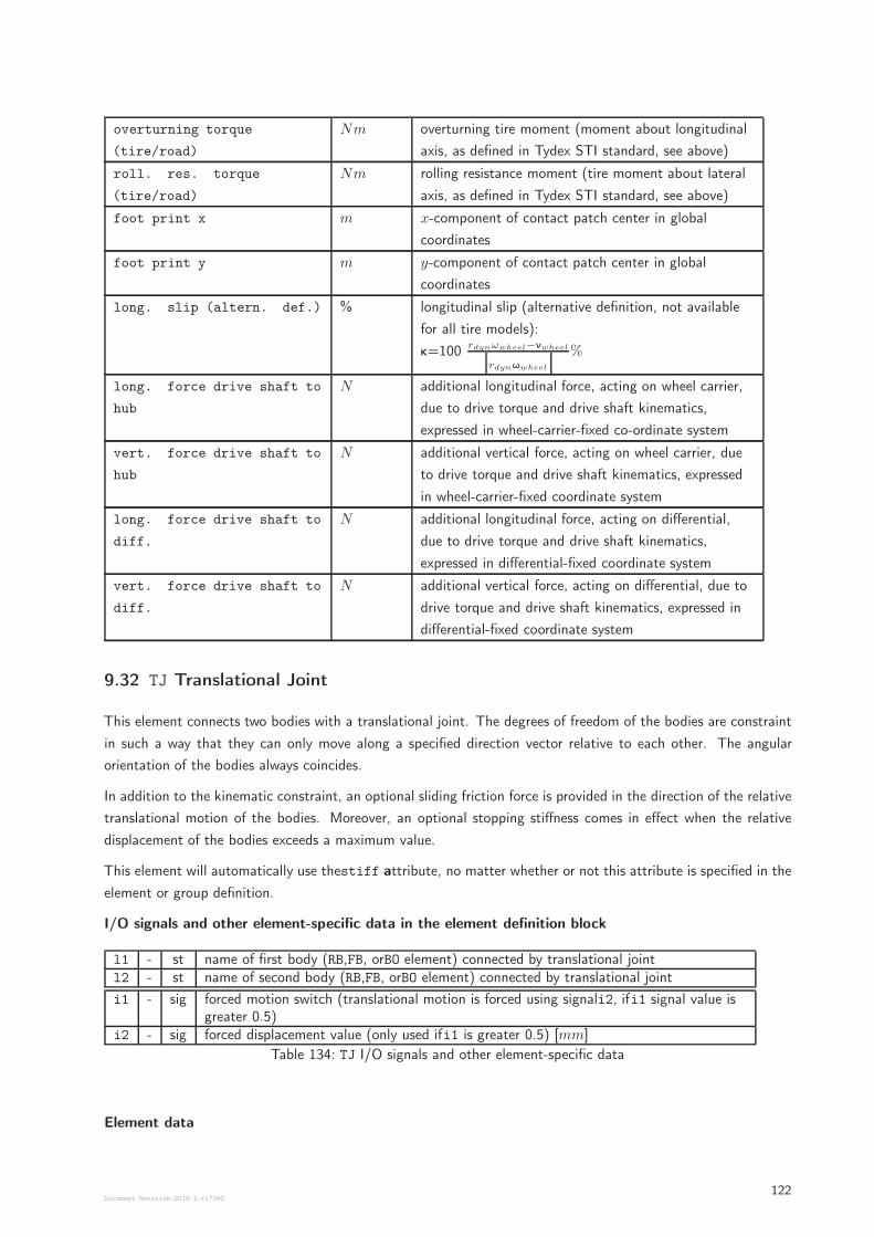
overturning torque
(tire/road)
Nm overturning tire moment (moment about longitudinal
axis, as defined in Tydex STI standard, see above)
roll. res. torque
(tire/road)
Nm rolling resistance moment (tire moment about lateral
axis, as defined in Tydex STI standard, see above)
foot print x m x-component of contact patch center in global
coordinates
foot print y m y-component of contact patch center in global
coordinates
long. slip (altern. def.) % longitudinal slip (alternative definition, not available
for all tire models):
κ=100rdynωwheel−νwheel
rdynωwheel
%
long. force drive shaft to
hub
N additional longitudinal force, acting on wheel carrier,
due to drive torque and drive shaft kinematics,
expressed in wheel-carrier-fixed co-ordinate system
vert. force drive shaft to
hub
N additional vertical force, acting on wheel carrier, due
to drive torque and drive shaft kinematics, expressed
in wheel-carrier-fixed coordinate system
long. force drive shaft to
diff.
N additional longitudinal force, acting on differential,
due to drive torque and drive shaft kinematics,
expressed in differential-fixed coordinate system
vert. force drive shaft to
diff.
N additional vertical force, acting on differential, due to
drive torque and drive shaft kinematics, expressed in
differential-fixed coordinate system
9.32 TJ Translational Joint
This element connects two bodies with a translational joint. The degrees of freedom of the bodies are constraint
in such a way that they can only move along a specified direction vector relative to each other. The angular
orientation of the bodies always coincides.
In addition to the kinematic constraint, an optional sliding friction force is provided in the direction of the relative
translational motion of the bodies. Moreover, an optional stopping stiffness comes in effect when the relative
displacement of the bodies exceeds a maximum value.
This element will automatically use thestiff attribute, no matter whether or not this attribute is specified in the
element or group definition.
I/O signals and other element-specific data in the element definition block
l1 - st name of first body (RB,FB, orBO element) connected by translational jointl2 - st name of second body (RB,FB, orBO element) connected by translational joint
i1 - sig forced motion switch (translational motion is forced using signali2, ifi1 signal value isgreater 0.5)
i2 - sig forced displacement value (only used ifi1 is greater 0.5) [mm]
Table 134: TJ I/O signals and other element-specific data
Element data
Document Revision:2018-2-r17342122
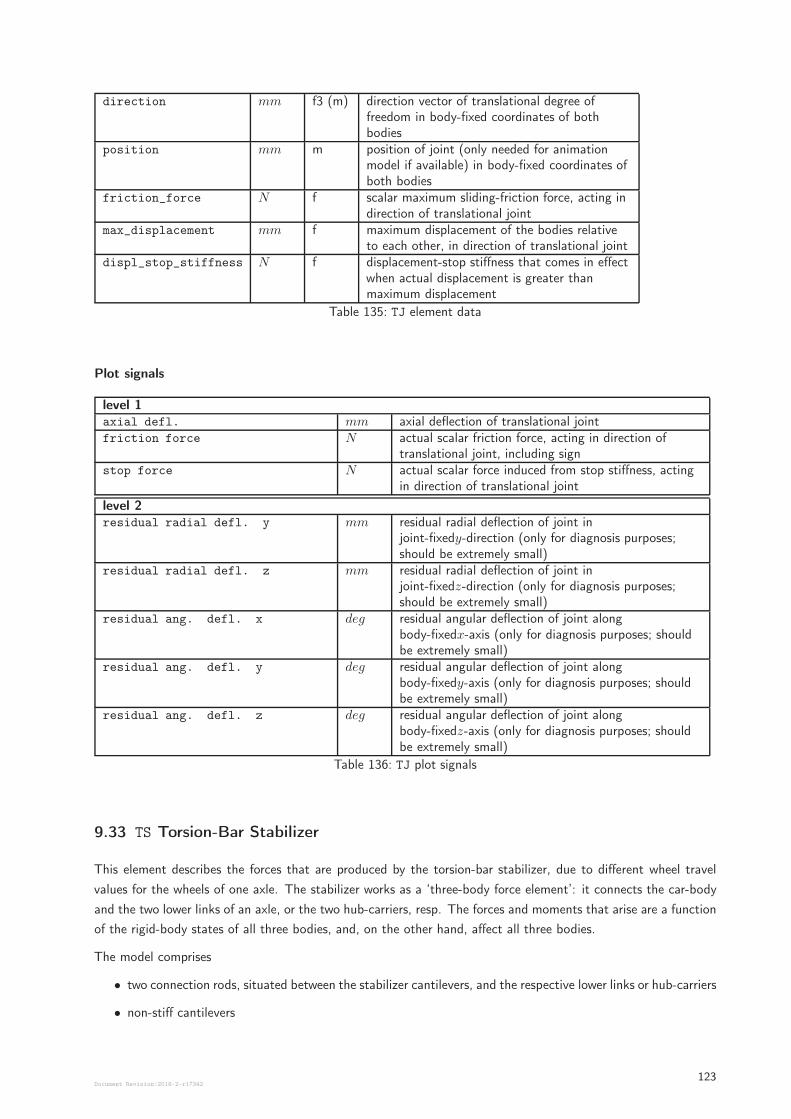
direction mm f3 (m) direction vector of translational degree offreedom in body-fixed coordinates of bothbodies
position mm m position of joint (only needed for animationmodel if available) in body-fixed coordinates ofboth bodies
friction_force N f scalar maximum sliding-friction force, acting indirection of translational joint
max_displacement mm f maximum displacement of the bodies relativeto each other, in direction of translational joint
displ_stop_stiffness N f displacement-stop stiffness that comes in effectwhen actual displacement is greater thanmaximum displacement
Table 135: TJ element data
Plot signals
level 1axial defl. mm axial deflection of translational jointfriction force N actual scalar friction force, acting in direction of
translational joint, including signstop force N actual scalar force induced from stop stiffness, acting
in direction of translational joint
level 2residual radial defl. y mm residual radial deflection of joint in
joint-fixedy-direction (only for diagnosis purposes;should be extremely small)
residual radial defl. z mm residual radial deflection of joint injoint-fixedz-direction (only for diagnosis purposes;should be extremely small)
residual ang. defl. x deg residual angular deflection of joint alongbody-fixedx-axis (only for diagnosis purposes; shouldbe extremely small)
residual ang. defl. y deg residual angular deflection of joint alongbody-fixedy-axis (only for diagnosis purposes; shouldbe extremely small)
residual ang. defl. z deg residual angular deflection of joint alongbody-fixedz-axis (only for diagnosis purposes; shouldbe extremely small)
Table 136: TJ plot signals
9.33 TS Torsion-Bar Stabilizer
This element describes the forces that are produced by the torsion-bar stabilizer, due to different wheel travel
values for the wheels of one axle. The stabilizer works as a ‘three-body force element’: it connects the car-body
and the two lower links of an axle, or the two hub-carriers, resp. The forces and moments that arise are a function
of the rigid-body states of all three bodies, and, on the other hand, affect all three bodies.
The model comprises
• two connection rods, situated between the stabilizer cantilevers, and the respective lower links or hub-carriers
• non-stiff cantilevers
Document Revision:2018-2-r17342123
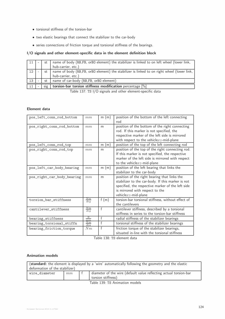
• torsional stiffness of the torsion-bar
• two elastic bearings that connect the stabilizer to the car-body
• series connections of friction torque and torsional stiffness of the bearings.
I/O signals and other element-specific data in the element definition block
l1 - st name of body (RB,FB, orBO element) the stabilizer is linked to on left wheel (lower link,hub-carrier, etc.)
l2 - st name of body (RB,FB, orBO element) the stabilizer is linked to on right wheel (lower link,hub-carrier, etc.)
l3 - st name of car-body (RB,FB, orBO element)
i1 - sig torsion-bar torsion stiffness modification percentage [%]
Table 137: TS I/O signals and other element-specific data
Element data
pos_left_conn_rod_bottom mm m (m) position of the bottom of the left connectingrod
pos_right_conn_rod_bottom mm m position of the bottom of the right connectingrod. If this marker is not specified, therespective marker of the left side is mirroredwith respect to the vehiclexz-mid-plane
pos_left_conn_rod_top mm m (m) position of the top of the left connecting rodpos_right_conn_rod_top mm m position of the top of the right connecting rod.
If this marker is not specified, the respectivemarker of the left side is mirrored with respectto the vehiclexz-mid-plane
pos_left_car_body_bearing mm m (m) position of the left bearing that links thestabilizer to the car-body
pos_right_car_body_bearing mm m position of the right bearing that links thestabilizer to the car-body. If this marker is notspecified, the respective marker of the left sideis mirrored with respect to thevehiclexz-mid-plane
torsion_bar_stiffness Nmdeg
f (m) torsion-bar torsional stiffness, without effect ofthe cantilevers
cantilever_stiffness Nmdeg
f cantilever stiffness, described by a torsionalstiffness in series to the torsion-bar stiffness
bearing_stiffness Nmm
f radial stiffness of the stabilizer bearings
bearing_torsional_stiffn Nmdeg
f torsional stiffness of the stabilizer bearings
bearing_friction_torque Nm f friction torque of the stabilizer bearings,situated in-line with the torsional stiffness
Table 138: TS element data
Animation models
(standard: the element is displayed by a ‘wire’ automatically following the geometry and the elasticdeformation of the stabilizer)wire_diameter mm f diameter of the wire (default value reflecting actual torsion-bar
torsion stiffness)
Table 139: TS Animation models
Document Revision:2018-2-r17342124
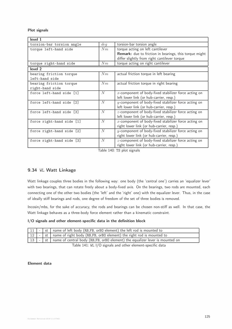
Plot signals
level 1torsion-bar torsion angle deg torsion-bar torsion angletorque left-hand side Nm torque acting on left cantilever
Remark: due to friction in bearings, this torque mightdiffer slightly from right cantilever torque
torque right-hand side Nm torque acting on right cantilever
level 2bearing friction torque
left-hand side
Nm actual friction torque in left bearing
bearing friction torque
right-hand side
Nm actual friction torque in right bearing
force left-hand side [1] N x-component of body-fixed stabilizer force acting onleft lower link (or hub-carrier, resp.)
force left-hand side [2] N y-component of body-fixed stabilizer force acting onleft lower link (or hub-carrier, resp.)
force left-hand side [3] N z-component of body-fixed stabilizer force acting onleft lower link (or hub-carrier, resp.)
force right-hand side [1] N x-component of body-fixed stabilizer force acting onright lower link (or hub-carrier, resp.)
force right-hand side [2] N y-component of body-fixed stabilizer force acting onright lower link (or hub-carrier, resp.)
force right-hand side [3] N z-component of body-fixed stabilizer force acting onright lower link (or hub-carrier, resp.)
Table 140: TS plot signals
9.34 WL Watt Linkage
Watt linkage couples three bodies in the following way: one body (the ‘central one’) carries an ‘equalizer lever’
with two bearings, that can rotate freely about a body-fixed axis. On the bearings, two rods are mounted, each
connecting one of the other two bodies (the ‘left’ and the ‘right’ one) with the equalizer lever. Thus, in the case
of ideally stiff bearings and rods, one degree of freedom of the set of three bodies is removed.
Incosin/mbs, for the sake of accuracy, the rods and bearings can be chosen non-stiff as well. In that case, the
Watt linkage behaves as a three-body force element rather than a kinematic constraint.
I/O signals and other element-specific data in the definition block
l1 - st name of left body (RB,FB, orBO element) the left rod is mounted tol2 - st name of right body (RB,FB, orBO element) the right rod is mounted tol3 - st name of central body (RB,FB, orBO element) the equalizer lever is mounted on
Table 141: WL I/O signals and other element-specific data
Element data
Document Revision:2018-2-r17342125
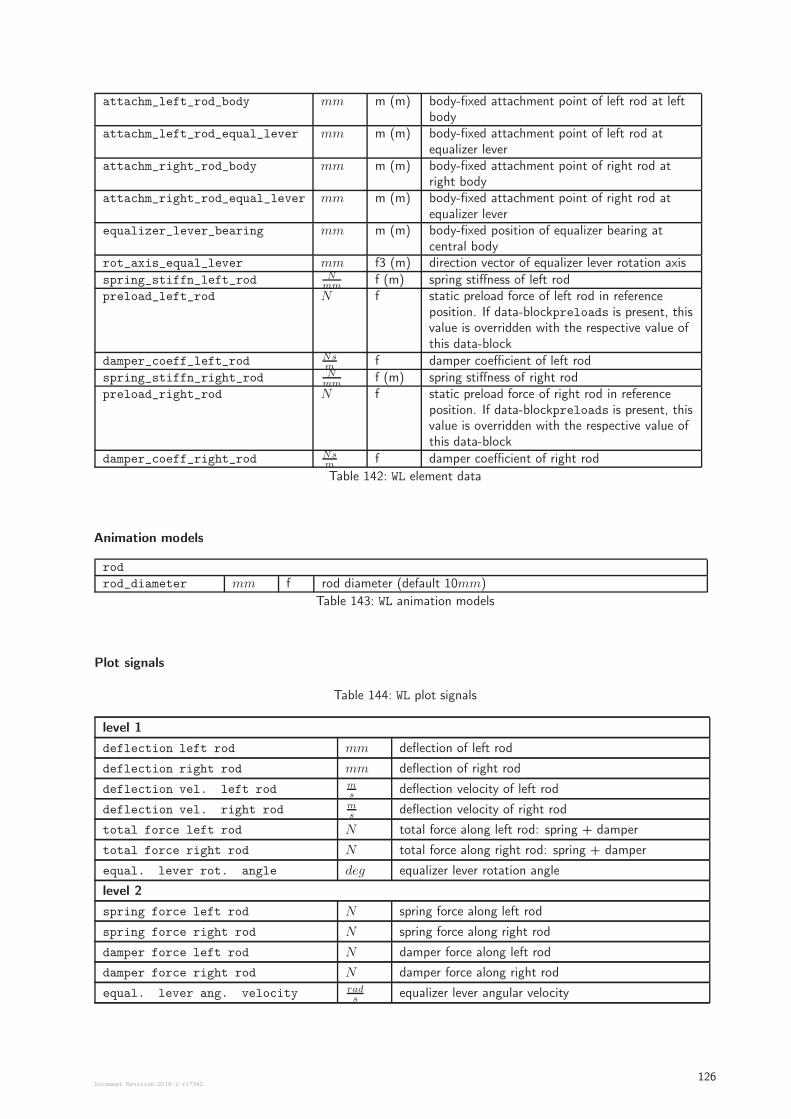
attachm_left_rod_body mm m (m) body-fixed attachment point of left rod at leftbody
attachm_left_rod_equal_lever mm m (m) body-fixed attachment point of left rod atequalizer lever
attachm_right_rod_body mm m (m) body-fixed attachment point of right rod atright body
attachm_right_rod_equal_lever mm m (m) body-fixed attachment point of right rod atequalizer lever
equalizer_lever_bearing mm m (m) body-fixed position of equalizer bearing atcentral body
rot_axis_equal_lever mm f3 (m) direction vector of equalizer lever rotation axis
spring_stiffn_left_rod Nmm
f (m) spring stiffness of left rodpreload_left_rod N f static preload force of left rod in reference
position. If data-blockpreloads is present, thisvalue is overridden with the respective value ofthis data-block
damper_coeff_left_rod Nsm
f damper coefficient of left rod
spring_stiffn_right_rod Nmm
f (m) spring stiffness of right rodpreload_right_rod N f static preload force of right rod in reference
position. If data-blockpreloads is present, thisvalue is overridden with the respective value ofthis data-block
damper_coeff_right_rod Nsm
f damper coefficient of right rod
Table 142: WL element data
Animation models
rod
rod_diameter mm f rod diameter (default 10mm)
Table 143: WL animation models
Plot signals
Table 144: WL plot signals
level 1
deflection left rod mm deflection of left rod
deflection right rod mm deflection of right rod
deflection vel. left rod ms
deflection velocity of left rod
deflection vel. right rod ms
deflection velocity of right rod
total force left rod N total force along left rod: spring + damper
total force right rod N total force along right rod: spring + damper
equal. lever rot. angle deg equalizer lever rotation angle
level 2
spring force left rod N spring force along left rod
spring force right rod N spring force along right rod
damper force left rod N damper force along left rod
damper force right rod N damper force along right rod
equal. lever ang. velocity rads
equalizer lever angular velocity
Document Revision:2018-2-r17342126
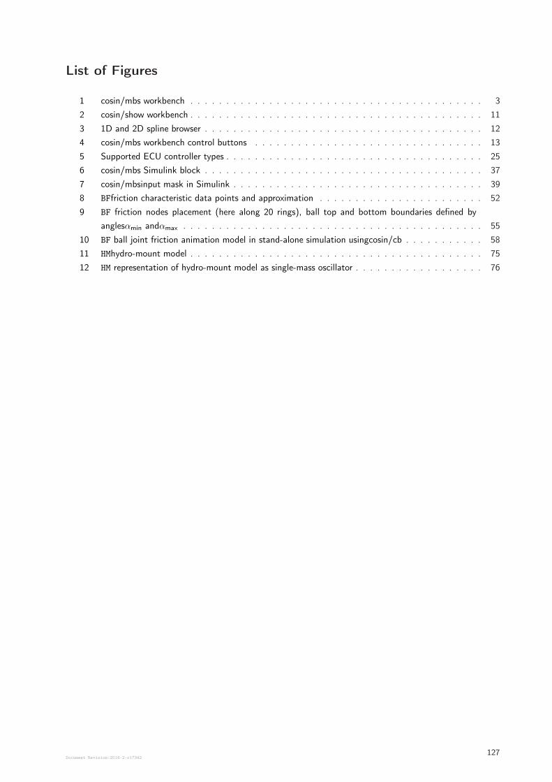
List of Figures
1 cosin/mbs workbench . . . . . . . . . . . . . . . . . . . . . . . . . . . . . . . . . . . . . . . . . 3
2 cosin/show workbench . . . . . . . . . . . . . . . . . . . . . . . . . . . . . . . . . . . . . . . . . 11
3 1D and 2D spline browser . . . . . . . . . . . . . . . . . . . . . . . . . . . . . . . . . . . . . . . 12
4 cosin/mbs workbench control buttons . . . . . . . . . . . . . . . . . . . . . . . . . . . . . . . . 13
5 Supported ECU controller types . . . . . . . . . . . . . . . . . . . . . . . . . . . . . . . . . . . . 25
6 cosin/mbs Simulink block . . . . . . . . . . . . . . . . . . . . . . . . . . . . . . . . . . . . . . . 37
7 cosin/mbsinput mask in Simulink . . . . . . . . . . . . . . . . . . . . . . . . . . . . . . . . . . . 39
8 BFfriction characteristic data points and approximation . . . . . . . . . . . . . . . . . . . . . . . 52
9 BF friction nodes placement (here along 20 rings), ball top and bottom boundaries defined by
anglesαmin andαmax . . . . . . . . . . . . . . . . . . . . . . . . . . . . . . . . . . . . . . . . . . 55
10 BF ball joint friction animation model in stand-alone simulation usingcosin/cb . . . . . . . . . . . 58
11 HMhydro-mount model . . . . . . . . . . . . . . . . . . . . . . . . . . . . . . . . . . . . . . . . . 75
12 HM representation of hydro-mount model as single-mass oscillator . . . . . . . . . . . . . . . . . . 76
Document Revision:2018-2-r17342127
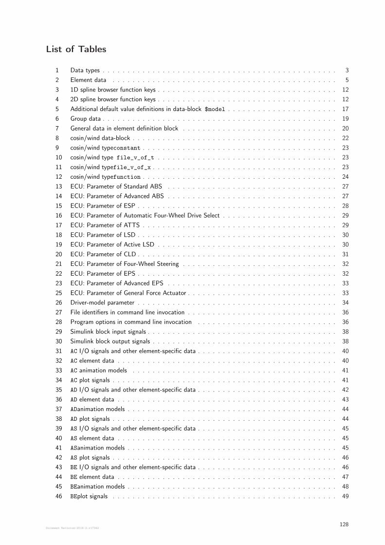
List of Tables
1 Data types . . . . . . . . . . . . . . . . . . . . . . . . . . . . . . . . . . . . . . . . . . . . . . . 3
2 Element data . . . . . . . . . . . . . . . . . . . . . . . . . . . . . . . . . . . . . . . . . . . . . 5
3 1D spline browser function keys . . . . . . . . . . . . . . . . . . . . . . . . . . . . . . . . . . . . 12
4 2D spline browser function keys . . . . . . . . . . . . . . . . . . . . . . . . . . . . . . . . . . . . 12
5 Additional default value definitions in data-block $model . . . . . . . . . . . . . . . . . . . . . . 17
6 Group data . . . . . . . . . . . . . . . . . . . . . . . . . . . . . . . . . . . . . . . . . . . . . . . 19
7 General data in element definition block . . . . . . . . . . . . . . . . . . . . . . . . . . . . . . . 20
8 cosin/wind data-block . . . . . . . . . . . . . . . . . . . . . . . . . . . . . . . . . . . . . . . . . 22
9 cosin/wind typeconstant . . . . . . . . . . . . . . . . . . . . . . . . . . . . . . . . . . . . . . . 23
10 cosin/wind type file_v_of_t . . . . . . . . . . . . . . . . . . . . . . . . . . . . . . . . . . . . 23
11 cosin/wind typefile_v_of_x . . . . . . . . . . . . . . . . . . . . . . . . . . . . . . . . . . . . . 23
12 cosin/wind typefunction . . . . . . . . . . . . . . . . . . . . . . . . . . . . . . . . . . . . . . . 24
13 ECU: Parameter of Standard ABS . . . . . . . . . . . . . . . . . . . . . . . . . . . . . . . . . . 27
14 ECU: Parameter of Advanced ABS . . . . . . . . . . . . . . . . . . . . . . . . . . . . . . . . . . 27
15 ECU: Parameter of ESP . . . . . . . . . . . . . . . . . . . . . . . . . . . . . . . . . . . . . . . . 28
16 ECU: Parameter of Automatic Four-Wheel Drive Select . . . . . . . . . . . . . . . . . . . . . . . 29
17 ECU: Parameter of ATTS . . . . . . . . . . . . . . . . . . . . . . . . . . . . . . . . . . . . . . . 29
18 ECU: Parameter of LSD . . . . . . . . . . . . . . . . . . . . . . . . . . . . . . . . . . . . . . . . 30
19 ECU: Parameter of Active LSD . . . . . . . . . . . . . . . . . . . . . . . . . . . . . . . . . . . . 30
20 ECU: Parameter of CLD . . . . . . . . . . . . . . . . . . . . . . . . . . . . . . . . . . . . . . . . 31
21 ECU: Parameter of Four-Wheel Steering . . . . . . . . . . . . . . . . . . . . . . . . . . . . . . . 32
22 ECU: Parameter of EPS . . . . . . . . . . . . . . . . . . . . . . . . . . . . . . . . . . . . . . . . 32
23 ECU: Parameter of Advanced EPS . . . . . . . . . . . . . . . . . . . . . . . . . . . . . . . . . . 33
25 ECU: Parameter of General Force Actuator . . . . . . . . . . . . . . . . . . . . . . . . . . . . . . 33
26 Driver-model parameter . . . . . . . . . . . . . . . . . . . . . . . . . . . . . . . . . . . . . . . . 34
27 File identifiers in command line invocation . . . . . . . . . . . . . . . . . . . . . . . . . . . . . . 36
28 Program options in command line invocation . . . . . . . . . . . . . . . . . . . . . . . . . . . . 36
29 Simulink block input signals . . . . . . . . . . . . . . . . . . . . . . . . . . . . . . . . . . . . . . 38
30 Simulink block output signals . . . . . . . . . . . . . . . . . . . . . . . . . . . . . . . . . . . . . 38
31 AC I/O signals and other element-specific data . . . . . . . . . . . . . . . . . . . . . . . . . . . . 40
32 AC element data . . . . . . . . . . . . . . . . . . . . . . . . . . . . . . . . . . . . . . . . . . . . 40
33 AC animation models . . . . . . . . . . . . . . . . . . . . . . . . . . . . . . . . . . . . . . . . . 41
34 AC plot signals . . . . . . . . . . . . . . . . . . . . . . . . . . . . . . . . . . . . . . . . . . . . . 41
35 AD I/O signals and other element-specific data . . . . . . . . . . . . . . . . . . . . . . . . . . . . 42
36 AD element data . . . . . . . . . . . . . . . . . . . . . . . . . . . . . . . . . . . . . . . . . . . . 43
37 ADanimation models . . . . . . . . . . . . . . . . . . . . . . . . . . . . . . . . . . . . . . . . . . 44
38 AD plot signals . . . . . . . . . . . . . . . . . . . . . . . . . . . . . . . . . . . . . . . . . . . . . 44
39 AS I/O signals and other element-specific data . . . . . . . . . . . . . . . . . . . . . . . . . . . . 45
40 AS element data . . . . . . . . . . . . . . . . . . . . . . . . . . . . . . . . . . . . . . . . . . . . 45
41 ASanimation models . . . . . . . . . . . . . . . . . . . . . . . . . . . . . . . . . . . . . . . . . . 45
42 AS plot signals . . . . . . . . . . . . . . . . . . . . . . . . . . . . . . . . . . . . . . . . . . . . . 46
43 BE I/O signals and other element-specific data . . . . . . . . . . . . . . . . . . . . . . . . . . . . 46
44 BE element data . . . . . . . . . . . . . . . . . . . . . . . . . . . . . . . . . . . . . . . . . . . . 47
45 BEanimation models . . . . . . . . . . . . . . . . . . . . . . . . . . . . . . . . . . . . . . . . . . 48
46 BEplot signals . . . . . . . . . . . . . . . . . . . . . . . . . . . . . . . . . . . . . . . . . . . . . 49
Document Revision:2018-2-r17342128
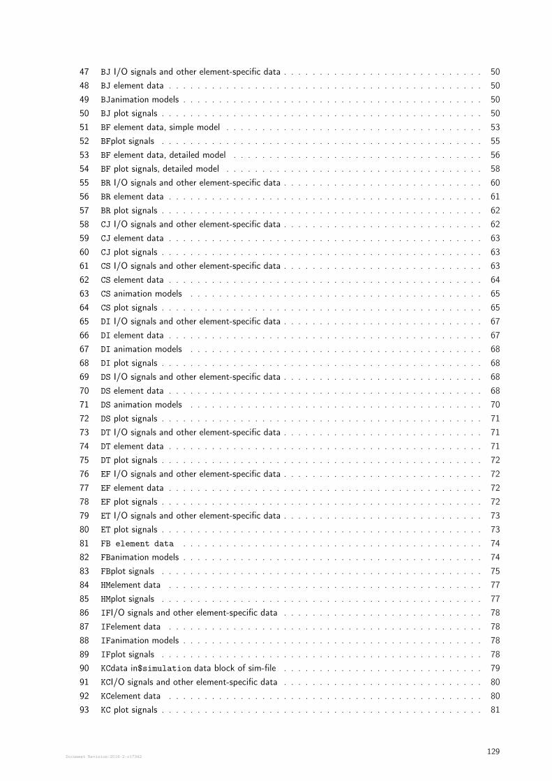
47 BJ I/O signals and other element-specific data . . . . . . . . . . . . . . . . . . . . . . . . . . . . 50
48 BJ element data . . . . . . . . . . . . . . . . . . . . . . . . . . . . . . . . . . . . . . . . . . . . 50
49 BJanimation models . . . . . . . . . . . . . . . . . . . . . . . . . . . . . . . . . . . . . . . . . . 50
50 BJ plot signals . . . . . . . . . . . . . . . . . . . . . . . . . . . . . . . . . . . . . . . . . . . . . 50
51 BF element data, simple model . . . . . . . . . . . . . . . . . . . . . . . . . . . . . . . . . . . . 53
52 BFplot signals . . . . . . . . . . . . . . . . . . . . . . . . . . . . . . . . . . . . . . . . . . . . . 55
53 BF element data, detailed model . . . . . . . . . . . . . . . . . . . . . . . . . . . . . . . . . . . 56
54 BF plot signals, detailed model . . . . . . . . . . . . . . . . . . . . . . . . . . . . . . . . . . . . 58
55 BR I/O signals and other element-specific data . . . . . . . . . . . . . . . . . . . . . . . . . . . . 60
56 BR element data . . . . . . . . . . . . . . . . . . . . . . . . . . . . . . . . . . . . . . . . . . . . 61
57 BR plot signals . . . . . . . . . . . . . . . . . . . . . . . . . . . . . . . . . . . . . . . . . . . . . 62
58 CJ I/O signals and other element-specific data . . . . . . . . . . . . . . . . . . . . . . . . . . . . 62
59 CJ element data . . . . . . . . . . . . . . . . . . . . . . . . . . . . . . . . . . . . . . . . . . . . 63
60 CJ plot signals . . . . . . . . . . . . . . . . . . . . . . . . . . . . . . . . . . . . . . . . . . . . . 63
61 CS I/O signals and other element-specific data . . . . . . . . . . . . . . . . . . . . . . . . . . . . 63
62 CS element data . . . . . . . . . . . . . . . . . . . . . . . . . . . . . . . . . . . . . . . . . . . . 64
63 CS animation models . . . . . . . . . . . . . . . . . . . . . . . . . . . . . . . . . . . . . . . . . 65
64 CS plot signals . . . . . . . . . . . . . . . . . . . . . . . . . . . . . . . . . . . . . . . . . . . . . 65
65 DI I/O signals and other element-specific data . . . . . . . . . . . . . . . . . . . . . . . . . . . . 67
66 DI element data . . . . . . . . . . . . . . . . . . . . . . . . . . . . . . . . . . . . . . . . . . . . 67
67 DI animation models . . . . . . . . . . . . . . . . . . . . . . . . . . . . . . . . . . . . . . . . . 68
68 DI plot signals . . . . . . . . . . . . . . . . . . . . . . . . . . . . . . . . . . . . . . . . . . . . . 68
69 DS I/O signals and other element-specific data . . . . . . . . . . . . . . . . . . . . . . . . . . . . 68
70 DS element data . . . . . . . . . . . . . . . . . . . . . . . . . . . . . . . . . . . . . . . . . . . . 68
71 DS animation models . . . . . . . . . . . . . . . . . . . . . . . . . . . . . . . . . . . . . . . . . 70
72 DS plot signals . . . . . . . . . . . . . . . . . . . . . . . . . . . . . . . . . . . . . . . . . . . . . 71
73 DT I/O signals and other element-specific data . . . . . . . . . . . . . . . . . . . . . . . . . . . . 71
74 DT element data . . . . . . . . . . . . . . . . . . . . . . . . . . . . . . . . . . . . . . . . . . . . 71
75 DT plot signals . . . . . . . . . . . . . . . . . . . . . . . . . . . . . . . . . . . . . . . . . . . . . 72
76 EF I/O signals and other element-specific data . . . . . . . . . . . . . . . . . . . . . . . . . . . . 72
77 EF element data . . . . . . . . . . . . . . . . . . . . . . . . . . . . . . . . . . . . . . . . . . . . 72
78 EF plot signals . . . . . . . . . . . . . . . . . . . . . . . . . . . . . . . . . . . . . . . . . . . . . 72
79 ET I/O signals and other element-specific data . . . . . . . . . . . . . . . . . . . . . . . . . . . . 73
80 ET plot signals . . . . . . . . . . . . . . . . . . . . . . . . . . . . . . . . . . . . . . . . . . . . . 73
81 FB element data . . . . . . . . . . . . . . . . . . . . . . . . . . . . . . . . . . . . . . . . . . 74
82 FBanimation models . . . . . . . . . . . . . . . . . . . . . . . . . . . . . . . . . . . . . . . . . . 74
83 FBplot signals . . . . . . . . . . . . . . . . . . . . . . . . . . . . . . . . . . . . . . . . . . . . . 75
84 HMelement data . . . . . . . . . . . . . . . . . . . . . . . . . . . . . . . . . . . . . . . . . . . . 77
85 HMplot signals . . . . . . . . . . . . . . . . . . . . . . . . . . . . . . . . . . . . . . . . . . . . . 77
86 IFI/O signals and other element-specific data . . . . . . . . . . . . . . . . . . . . . . . . . . . . 78
87 IFelement data . . . . . . . . . . . . . . . . . . . . . . . . . . . . . . . . . . . . . . . . . . . . 78
88 IFanimation models . . . . . . . . . . . . . . . . . . . . . . . . . . . . . . . . . . . . . . . . . . 78
89 IFplot signals . . . . . . . . . . . . . . . . . . . . . . . . . . . . . . . . . . . . . . . . . . . . . 78
90 KCdata in$simulation data block of sim-file . . . . . . . . . . . . . . . . . . . . . . . . . . . . 79
91 KCI/O signals and other element-specific data . . . . . . . . . . . . . . . . . . . . . . . . . . . . 80
92 KCelement data . . . . . . . . . . . . . . . . . . . . . . . . . . . . . . . . . . . . . . . . . . . . 80
93 KC plot signals . . . . . . . . . . . . . . . . . . . . . . . . . . . . . . . . . . . . . . . . . . . . . 81
Document Revision:2018-2-r17342129
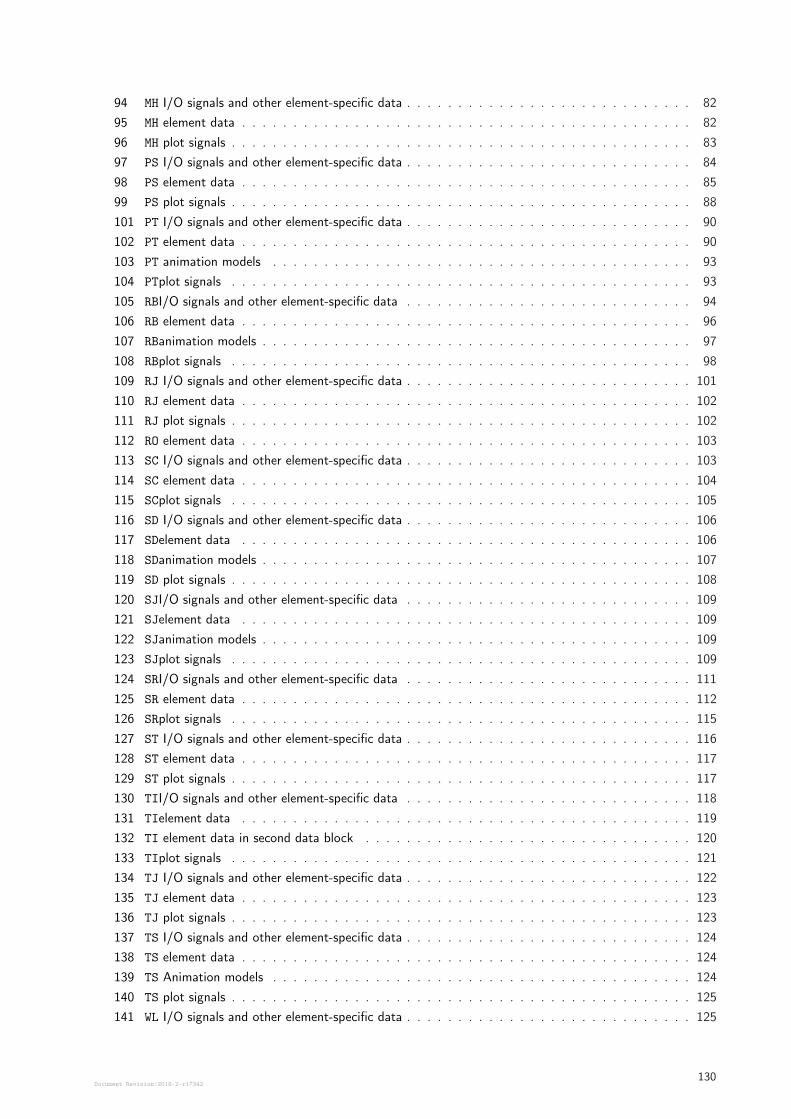
94 MH I/O signals and other element-specific data . . . . . . . . . . . . . . . . . . . . . . . . . . . . 82
95 MH element data . . . . . . . . . . . . . . . . . . . . . . . . . . . . . . . . . . . . . . . . . . . . 82
96 MH plot signals . . . . . . . . . . . . . . . . . . . . . . . . . . . . . . . . . . . . . . . . . . . . . 83
97 PS I/O signals and other element-specific data . . . . . . . . . . . . . . . . . . . . . . . . . . . . 84
98 PS element data . . . . . . . . . . . . . . . . . . . . . . . . . . . . . . . . . . . . . . . . . . . . 85
99 PS plot signals . . . . . . . . . . . . . . . . . . . . . . . . . . . . . . . . . . . . . . . . . . . . . 88
101 PT I/O signals and other element-specific data . . . . . . . . . . . . . . . . . . . . . . . . . . . . 90
102 PT element data . . . . . . . . . . . . . . . . . . . . . . . . . . . . . . . . . . . . . . . . . . . . 90
103 PT animation models . . . . . . . . . . . . . . . . . . . . . . . . . . . . . . . . . . . . . . . . . 93
104 PTplot signals . . . . . . . . . . . . . . . . . . . . . . . . . . . . . . . . . . . . . . . . . . . . . 93
105 RBI/O signals and other element-specific data . . . . . . . . . . . . . . . . . . . . . . . . . . . . 94
106 RB element data . . . . . . . . . . . . . . . . . . . . . . . . . . . . . . . . . . . . . . . . . . . . 96
107 RBanimation models . . . . . . . . . . . . . . . . . . . . . . . . . . . . . . . . . . . . . . . . . . 97
108 RBplot signals . . . . . . . . . . . . . . . . . . . . . . . . . . . . . . . . . . . . . . . . . . . . . 98
109 RJ I/O signals and other element-specific data . . . . . . . . . . . . . . . . . . . . . . . . . . . . 101
110 RJ element data . . . . . . . . . . . . . . . . . . . . . . . . . . . . . . . . . . . . . . . . . . . . 102
111 RJ plot signals . . . . . . . . . . . . . . . . . . . . . . . . . . . . . . . . . . . . . . . . . . . . . 102
112 RO element data . . . . . . . . . . . . . . . . . . . . . . . . . . . . . . . . . . . . . . . . . . . . 103
113 SC I/O signals and other element-specific data . . . . . . . . . . . . . . . . . . . . . . . . . . . . 103
114 SC element data . . . . . . . . . . . . . . . . . . . . . . . . . . . . . . . . . . . . . . . . . . . . 104
115 SCplot signals . . . . . . . . . . . . . . . . . . . . . . . . . . . . . . . . . . . . . . . . . . . . . 105
116 SD I/O signals and other element-specific data . . . . . . . . . . . . . . . . . . . . . . . . . . . . 106
117 SDelement data . . . . . . . . . . . . . . . . . . . . . . . . . . . . . . . . . . . . . . . . . . . . 106
118 SDanimation models . . . . . . . . . . . . . . . . . . . . . . . . . . . . . . . . . . . . . . . . . . 107
119 SD plot signals . . . . . . . . . . . . . . . . . . . . . . . . . . . . . . . . . . . . . . . . . . . . . 108
120 SJI/O signals and other element-specific data . . . . . . . . . . . . . . . . . . . . . . . . . . . . 109
121 SJelement data . . . . . . . . . . . . . . . . . . . . . . . . . . . . . . . . . . . . . . . . . . . . 109
122 SJanimation models . . . . . . . . . . . . . . . . . . . . . . . . . . . . . . . . . . . . . . . . . . 109
123 SJplot signals . . . . . . . . . . . . . . . . . . . . . . . . . . . . . . . . . . . . . . . . . . . . . 109
124 SRI/O signals and other element-specific data . . . . . . . . . . . . . . . . . . . . . . . . . . . . 111
125 SR element data . . . . . . . . . . . . . . . . . . . . . . . . . . . . . . . . . . . . . . . . . . . . 112
126 SRplot signals . . . . . . . . . . . . . . . . . . . . . . . . . . . . . . . . . . . . . . . . . . . . . 115
127 ST I/O signals and other element-specific data . . . . . . . . . . . . . . . . . . . . . . . . . . . . 116
128 ST element data . . . . . . . . . . . . . . . . . . . . . . . . . . . . . . . . . . . . . . . . . . . . 117
129 ST plot signals . . . . . . . . . . . . . . . . . . . . . . . . . . . . . . . . . . . . . . . . . . . . . 117
130 TII/O signals and other element-specific data . . . . . . . . . . . . . . . . . . . . . . . . . . . . 118
131 TIelement data . . . . . . . . . . . . . . . . . . . . . . . . . . . . . . . . . . . . . . . . . . . . 119
132 TI element data in second data block . . . . . . . . . . . . . . . . . . . . . . . . . . . . . . . . 120
133 TIplot signals . . . . . . . . . . . . . . . . . . . . . . . . . . . . . . . . . . . . . . . . . . . . . 121
134 TJ I/O signals and other element-specific data . . . . . . . . . . . . . . . . . . . . . . . . . . . . 122
135 TJ element data . . . . . . . . . . . . . . . . . . . . . . . . . . . . . . . . . . . . . . . . . . . . 123
136 TJ plot signals . . . . . . . . . . . . . . . . . . . . . . . . . . . . . . . . . . . . . . . . . . . . . 123
137 TS I/O signals and other element-specific data . . . . . . . . . . . . . . . . . . . . . . . . . . . . 124
138 TS element data . . . . . . . . . . . . . . . . . . . . . . . . . . . . . . . . . . . . . . . . . . . . 124
139 TS Animation models . . . . . . . . . . . . . . . . . . . . . . . . . . . . . . . . . . . . . . . . . 124
140 TS plot signals . . . . . . . . . . . . . . . . . . . . . . . . . . . . . . . . . . . . . . . . . . . . . 125
141 WL I/O signals and other element-specific data . . . . . . . . . . . . . . . . . . . . . . . . . . . . 125
Document Revision:2018-2-r17342130

142 WL element data . . . . . . . . . . . . . . . . . . . . . . . . . . . . . . . . . . . . . . . . . . . . 126
143 WL animation models . . . . . . . . . . . . . . . . . . . . . . . . . . . . . . . . . . . . . . . . . 126
144 WL plot signals . . . . . . . . . . . . . . . . . . . . . . . . . . . . . . . . . . . . . . . . . . . . . 126
Document Revision:2018-2-r17342131
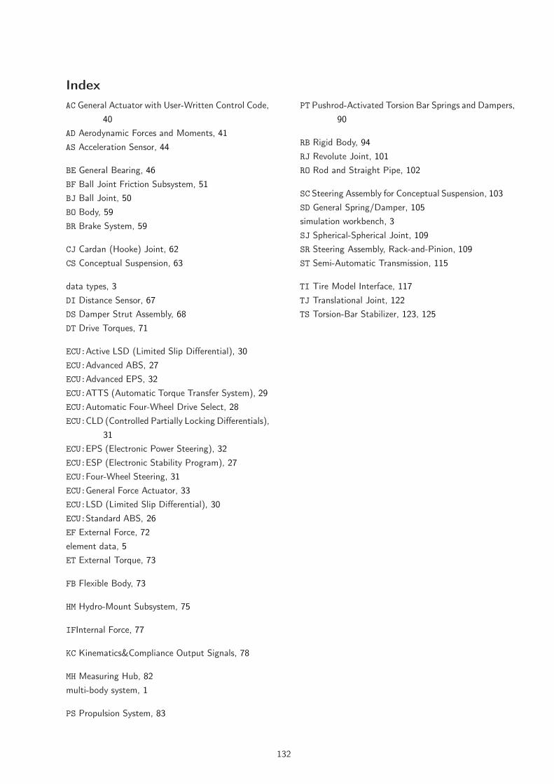
Index
AC General Actuator with User-Written Control Code,
40
AD Aerodynamic Forces and Moments, 41
AS Acceleration Sensor, 44
BE General Bearing, 46
BF Ball Joint Friction Subsystem, 51
BJ Ball Joint, 50
BO Body, 59
BR Brake System, 59
CJ Cardan (Hooke) Joint, 62
CS Conceptual Suspension, 63
data types, 3
DI Distance Sensor, 67
DS Damper Strut Assembly, 68
DT Drive Torques, 71
ECU:Active LSD (Limited Slip Differential), 30
ECU:Advanced ABS, 27
ECU:Advanced EPS, 32
ECU:ATTS (Automatic Torque Transfer System), 29
ECU:Automatic Four-Wheel Drive Select, 28
ECU:CLD (Controlled Partially Locking Differentials),
31
ECU:EPS (Electronic Power Steering), 32
ECU:ESP (Electronic Stability Program), 27
ECU:Four-Wheel Steering, 31
ECU:General Force Actuator, 33
ECU:LSD (Limited Slip Differential), 30
ECU:Standard ABS, 26
EF External Force, 72
element data, 5
ET External Torque, 73
FB Flexible Body, 73
HM Hydro-Mount Subsystem, 75
IFInternal Force, 77
KC Kinematics&Compliance Output Signals, 78
MH Measuring Hub, 82
multi-body system, 1
PS Propulsion System, 83
PT Pushrod-Activated Torsion Bar Springs and Dampers,
90
RB Rigid Body, 94
RJ Revolute Joint, 101
RO Rod and Straight Pipe, 102
SC Steering Assembly for Conceptual Suspension, 103
SD General Spring/Damper, 105
simulation workbench, 3
SJ Spherical-Spherical Joint, 109
SR Steering Assembly, Rack-and-Pinion, 109
ST Semi-Automatic Transmission, 115
TI Tire Model Interface, 117
TJ Translational Joint, 122
TS Torsion-Bar Stabilizer, 123, 125
132
Recommended