CODEN:LUTMDN/(TMMV-5270)/1-32/2015
CostAnalysisforCrushingandScreening–PartII
Developmentofacostmodelfordeterminationoftheproductioncostforproductfractions
Johan Fägerlind
Division of Production and Materials Engineering,
Lund University
2015
I
PrefaceThis Master thesis was performed during the spring of 2015 at Sandvik SRP AB in
Svedala as the end of the candidates’ education in Master of Science in Industrial
Engineering and Management.
Special thanks go to Per Hedvall as a supervisor at Sandvik SRP how has been a
great help throw‐out the entire process with this Master Thesis. I will also thank
all other supervisors Per Svedensten, Hamid Manouchehri and Fredrik Schultheiss.
Thanks to all other colleges at Sandvik SRP AB that have been helpful or just made
my day a little bit better.
I will of course like to thank Jan‐Eric Ståhl for his help, ideas and knowledge who
helpt me out during this study.
Finally I would like to send a grateful tank to my family and friends that have
supported me through my studies, without you it would not be possible.
Supervisors:
Hamid Manouchehri, Principal Advisor Sandvik SRP Per Svedensten, Manager Crushing Chambers and Material Development, Sandvik SRP Fredrik Schultheiss, Institution for Industrial Production Faculty of Engineering Lund University Per Hedvall, Senior Advisor, Sandvik SRP AB Examiner: Jan‐Eric Ståhl, Institution for Industrial Production Faculty of Engineering Svedala, June 29, 2015 Johan Fägerlind
II
AbstractSandvik SRP has earlier studied a new way of calculating the cost in crushing and
screening the results was a satisfactory, Sandvik SRP is now ready to go further in
this study.
The purpose of this study is further develop of the earlier adopted generic cost
model earlier developed by Heyman and Lindström in order to calculate the cost
per metric ton within the world of crushing and screening. By implementing the
cost calculation in Microsoft excel it would be more user friendly and applicable
when calculating the cost in crushing and screening.
The model by Hayman and Lindstöm is based on the macroeconomic generic cost‐
model, developed and published by Ståhl. Heyman and Lindstöm developed a
new model to fit the crushing and screening operations better. This model had
some issues according to the payroll cost and the deprecation cost which the
author now have solved in this study.
By implement the cost model in Microsoft Excel by using VBA (Visual Basic for
Application) the calculations and simulations can be easy to use when most of the
employees are well familiar with Microsoft Excel. To implement the model and to
programming all macros that is used is very time consuming and this is the largest
part of this study.
The results through this study were very accurate according to the results from
previous study but the validation was an issue. To validate this study the
comparison has been made with Heyman and Lindström results from the previous
study. They had such good results and a more quantitative study was not made
according to lack of time.
The recommendation from the results according to this study is to validate the
model even further and not at least for a construction site before further
implementation in for example Plant Designer etc.
III
TableofContentsPreface ....................................................................................................................... I
Abstract ..................................................................................................................... II
List of Figures ............................................................................................................ V
List of Tables ............................................................................................................. V
List of Equations ........................................................................................................ V
1. Introduction .......................................................................................................... 1
1.1 Company presentation.................................................................................... 1
1.1.1 Sandvik AB ................................................................................................ 1
1.1.2 Sandvik SRP AB Svedala ........................................................................... 2
1.1.3 Process ..................................................................................................... 2
1.2 Background ..................................................................................................... 3
1.3 Purpose and Goals .......................................................................................... 3
1.4 Delimitations ................................................................................................... 3
1.5 Report Structure ............................................................................................. 3
2. Methodology ......................................................................................................... 5
2.1 Approach ......................................................................................................... 5
2.2.1 Formulate the Problem ............................................................................ 6
2.2.2 Collect information/Data ......................................................................... 6
2.2.3 Concept and building the model .............................................................. 6
2.2.4 Result and Analysis of the Output ........................................................... 7
2.2.5 Finalizing .................................................................................................. 7
3. Theory ................................................................................................................... 8
3.1 The Generic Production Cost Model ............................................................... 8
3.1.1 Generic Production Cost Model ............................................................... 8
3.1.2 Earlier Adopted Production Cost Model .................................................. 8
3.1.3 New Adopted Production Cost Model ..................................................... 9
3.2 Building of the new Adopted Production Cost Model in Excel ..................... 12

IV
3.2.1 Visual Basic for Applications .................................................................. 12
3.2.2 Interface ................................................................................................. 12
3.2.3 Output .................................................................................................... 13
3.2.5 User Manual ........................................................................................... 13
3.2.4 Assumptions ........................................................................................... 16
3.3 Mont‐Carlo Simulation .................................................................................. 17
4 Results .................................................................................................................. 18
4.1 ....................................................................................................................... 19
4.1.1 Raw material cost ................................................................................... 19
4.1.2 Payroll cost ............................................................................................. 19
4.1.3 Machine cost during uptime .................................................................. 19
4.1.4 Machine cost during downtime ............................................................. 20
4.1.5 Total production cost per metric ton ..................................................... 21
4.2 Result analysis ............................................................................................... 21
4.2.1 Total production cost ............................................................................. 21
4.2.2 Differences between calculations .......................................................... 22
5 Conclusions .......................................................................................................... 24
6 Further studies ..................................................................................................... 25
6 References ........................................................................................................... 26
Literature ............................................................................................................ 26
Articles ................................................................................................................ 26
Electronic resources ............................................................................................ 27
Interviews ............................................................................................................ 27
Appendix ................................................................................................................. 28
Appendix A ...................................................................................................... 28
Appendix B (Heyman and Lindström index) ....................................................... 29

V
ListofFigures
Figure 1: Sandvik business areas ............................................................................................ 1
Figure 2: Laws model .............................................................................................................. 5
Figure 3: The interface of the developed program ...............................................................14
Figure 4: Second part of the interface ..................................................................................15
Figure 5: Flow sheet over the production .............................................................................18
Figure 6: The results from the production cost calculations.................................................18
Figure 7: Payroll distribution function according to Heyman and Lindström .......................19
Figure 8: Distribution function over production cost during up‐time according to Heyman
and Lindström ......................................................................................................................20
Figure 9: Distribution function over production cost during down‐time according to
Heyman and Lindström ........................................................................................................20
Figure 10: Split over mining costs .........................................................................................22
Figure 8: Split over production cost when producing construction aggregates ...................22
ListofTables
Table 1: Total cost for production at the company according to this study .........................19
ListofEquations
Equation 1: Generic Production cost model ........................................................................... 8
Equation 2: Earlier adopted production cost model ............................................................... 9
Equation 3: New adopted production cost model ................................................................10
Equation 4: Production cost during up‐time .........................................................................11
Equation 5: Spare part caluclation .......................................................................................11
Equation 6: Production during down‐time ...........................................................................11
Equation 7: Balancing loss calculation .................................................................................11
1.Introduction
This chapter will present Sandvik Rock Processing (SRP) Ab different business
areas, give a short introduction as well as the background of this master thesis.
1.1Companypresentation
1.1.1SandvikAB12Sandvik AB was founded in 1862 by Göran Fredrik Göransson who was the first in
the world to use the Bessermermethod in the production of steel. The major
strategy at Sandvik since start is to be to top class in research and development.
Sandvik production is divided into five different business areas: Sandvik Mining,
Sandvik Machining Solutions, Sandvik materials Technology, Sandvik Construction
and Sandvik Venture. This study has been made on behalf of Sandvik Mining.
Figure 1: Sandvik business areas3
Sandvik is represented in over 130 countries and had a turnover in 2014 85.9
billion SEK.4
1 Sandvik.se 2 Sandvik Mining and Construction intranät Sverige 3 Sandvik Mining and Construction intranät Sverige 4 Sandvik årsredovisning, 2014

2
1.1.2SandvikSRPABSvedala5Sandvik SRP AB in Svedala was founded in 1882 by the name Åbjörn Andersson &
Co. Åbjörn Andersson himself was a blacksmith and in the beginning of Åbjörn
Andersson & Co. the production was mainly agricultural machinery and brickyard
equipment. Until the Russian revolution 1917 the brickyard equipment was the
largest cash‐cow for Åbjörn Andersson & Co. but when the Russian revolution
occurred the export to Russia died. Around 1900 Åbjörn Andersson & Co. has
started to produce a simple and transportable jaw‐crusher for farmers to produce
gravel for the earlier dirt roads. Paved roads became more and more important
when the people started using cars instead of horses for traveling therefore
Åbjörn Andersson & Co equipment became more popular. Åbjörn Andersson &
Co. developed even more equipment for road maintenance such as graders. The
road equipment developed during the early 1900 century and after the Second
World War Åbjörn Andersson & Co. begins to produce a cone crusher on contract
for Allis Chalmers. This was the start of what SRP is today. Åbjörn Andersson & Co.
has been in many company fusions and has also been bought by other companies,
but from 2001 Sandvik AB is the owner of the site in Svedala.
1.1.3Process
1.1.3.1ProductsSRP produce most of the equipment for the crushing and screening process jaw
crushers, cone crushers, gyratory crushers, HIS (High Speed Impact) and VSI
(Vertical Shaft Impact) crushers and screening equipment. In Svedala the
production is concentrated to jaw crushers and cone crushers.
1.1.3.2ProcessFlowThe process flow described in figure.. is a typical process flow built up by a
primary crushing stage, secondary crushing stage. The primary stage usually has a
jaw or a gyratory crusher and screening equipment. The secondary have a single
or several cone, VSI, HSI crushers and screening equipment. In a mining industry
the main idea is to reduce particle size until the mineral can be extracted out of
the ore. In construction the particle size is a lot more important when different
aggregates are used as several different construction materials.
5 ”Gjuteriet” 125 år, 2007
3
1.2BackgroundAs an attempt to develop a production cost model to forecast the costs for different crushed products in comminution plant a master project has been defined in collaboration between the division of Production and Materials Engineering of Lund University (LTH) and Sandvik Rock Processing (Sandvik SRP, Svedala). The first part of the project which has been completed during the spring 2014 resulted in developing of a primary model to be used to estimate/predict the cost for a single crushed product within a simple crushing/comminution circuit. However, there are needs to further develop the primary model to deal with more complicated crushing circuit in which more than one product is produced.
The main objective for the project is to develop a user‐friendly model for Sandvik Rock Processing (SRP) which will be used by sales engineers as a tool for predicting the cost(s) for the crushing projects to satisfy customers.
So far, the achieved results from the first part of the project have been satisfactory, encouraging Sandvik SRP to proceed further. This means the model must be developed in a way to enable us to estimate/predict the costs for different/multiple crushed products within a designed crushing circuit.
1.3PurposeandGoalsThe purpose of this master thesis will be further development of the Cost Analysis
for Crushing and Screening Model. The base of this project will be Cost Analysis
for Crushing and screening – Part I.
The final outcome will be to present a comprehensive users‐friendly model which can be implemented in the Microsoft Excel. This project will aim to get a result with <85% accuracy.
1.4DelimitationsFor this project there will be some delimitations:
‐ The costs before the crushing and screening stage are fixed (which
includes drilling, blasting and hauling).
‐ The costs after the crushing and screening stage are not included
(transportation out of the pit/mine etc.).
1.5ReportStructure
Chapter1–IntroductionThis first chapter will include a short presentation of the company, background,
purpose, goals and delimitations of this Master Thesis.

4
Chapter2–MethodologyIn the second chapter the methodology for this project is described.
Chapter3–TheoryIn the third chapter the theoretical models that have been used during the project
is described. The background according to the Generic Cost Model by Ståhl and
the Monte‐Carlo simulation models6 will be presented in this chapter.
Chapter4–CalculationmodelIn the fourth chapter the adopted Generic Cost Model that has been used within
the Excel program will be presented in detail.
Chapter5–ResultsIn the fifth chapter the result from this project will be presented together with the
validation of the program.
Chapter6–ConclusionsandRecommendationIn the sixth chapter the conclusions out of this project will be presented and also a
recommendation for further work to get an even more precise model.
Chapter7‐References
Chapter8‐Appendix
6 Development of manufacturing Systems, 2013
5
2.MethodologyThis chapter will present the different techniques and methods that have been
used for this project. The main point of this study is further development of The
Generic Production Cost Model by Ståhl to fit the crushing and screening process
even better than earlier studies.
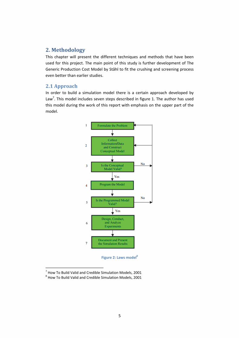
2.1ApproachIn order to build a simulation model there is a certain approach developed by
Law7. This model includes seven steps described in figure 1. The author has used
this model during the work of this report with emphasis on the upper part of the
model.
Figure 2: Laws model8
7 How To Build Valid and Credible Simulation Models, 2001 8 How To Build Valid and Credible Simulation Models, 2001
6
2.2.1FormulatetheProblemThe purpose and goals where defined and a project plan was made. All involved
parties had to approve the project plan9.
2.2.2Collectinformation/DataThere are two types of data, primary and secondary10. The primary data is the one
that the author himself collects and the secondary is the one already existing such
as earlier thesis etc. During the work with this thesis data collection has been
made throughout the whole process.
2.2.2.1LiteraturestudiesThe literature studies were mainly done by reading books, articles and other
master’s thesis.
2.2.2.2LecturesTo start off this project a lecture during three days were held. The purpose of the
lecture was to get a good view of the company and also a basic education in
process technology and Plant Designer.
2.2.2.3InterviewsThroughout the work with this project interviews were held. The interviews where
mostly dialog around areas where real data were impossible to get hold of. The
interviews were held at the Sandvik SRP AB site in Svedala.
2.2.3ConceptandbuildingthemodelThe concept of modeling is a simplification of reality to make it possible to analyze
a real case. The model makes it easy to look at several different scenarios. To
make the model three different parameters has to be taken in to account.11
‐ Delimitations – If the model is too large then it will be to complex and if
the model is too small then it the model might lose some important
aspects.
‐ Input/Output – The input that will affect the most should be prioritized.
The input is the varying variable and the output is the parameter that will
be analyzed.
9 Att genomföra examensarbete, 2006 10 Information för marknadsföringsbeslut, 2001 11 Att genomföra examensarbete, 2006
7
‐ Level of abstractness – If the model is very detailed the model it will catch
all the different aspects but it will also make the model to complex and
there is a risk that some of the input variables doesn’t affect the output.
Building the model and collection of data is the most time consuming part of the
project.
2.2.4ResultandAnalysisoftheOutputThe result will mostly be analyzed from the authors own thoughts and
experiences, so if the reader shall be able to make own conclusions the material
has to be well documented.12
2.2.5FinalizingThe ending of this Master Thesis means that the final touches are made and it will
be presented for Sandvik AB and the institution.
12 Seminarieboken – att skriva, presentera och opponera, 2003
8
3.Theory
3.1TheGenericProductionCostModelThe following models will include plenty of formulas which the reader will find in
appendix.
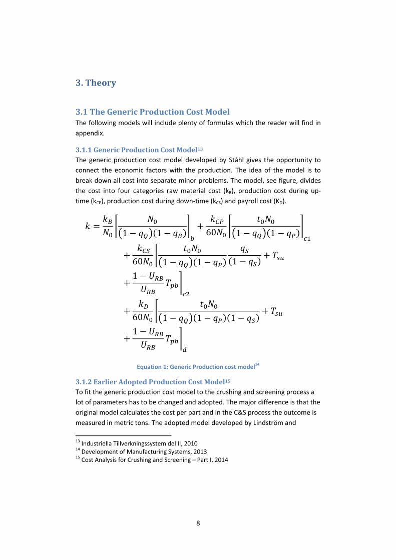
3.1.1GenericProductionCostModel13The generic production cost model developed by Ståhl gives the opportunity to
connect the economic factors with the production. The idea of the model is to
break down all cost into separate minor problems. The model, see figure, divides
the cost into four categories raw material cost (kB), production cost during up‐
time (kCP), production cost during down‐time (kCS) and payroll cost (KD).
1 1
60 1 1
60 1 1 1
1
60 1 1 11
Equation 1: Generic Production cost model14
3.1.2EarlierAdoptedProductionCostModel15To fit the generic production cost model to the crushing and screening process a
lot of parameters has to be changed and adopted. The major difference is that the
original model calculates the cost per part and in the C&S process the outcome is
measured in metric tons. The adopted model developed by Lindström and
13 Industriella Tillverkningssystem del II, 2010 14 Development of Manufacturing Systems, 2013 15 Cost Analysis for Crushing and Screening – Part I, 2014

9
Heyman is presented below. This model was the base of the new adopted
production cost model which will be presented in the next chapter in detail.
1
∙
∙ ∙1 1
∙ ∙
1 1 1
1 ∙ ∙1 1 1
∙ ∙1 1 1
1 ∙ ∙1 1 1
Equation 2: Earlier adopted production cost model16
3.1.3NewAdoptedProductionCostModelThe major goal of this study is to make a user‐friendly program that can be used
by many of the company’s employees and applicable for all different kind of sites.
This will cause that the new model to be a little bit less detailed. If all details in the
previous model shall be included the level of user‐friendliness would decrease
that much that the model might not be used in the extend Sandvik would like.
The major differences:
1. Tsu = 0, this is done due to the fact that the setup time is included in the
wear part cost and in the deprecation cost.
2. The material flow is replaced with a better calculated balancing loss.
16 Cost Analysis for Crushing and Screening – Part I, 2014

10
∙
1 1
1 1 1
11 1 1
1 1 1
11 1 1
Equation 3: New adopted production cost model
3.1.3.1Costpermetrictonkj17In earlier studies the generic cost model has to be changed to calculate the cost
per metric ton instead of the production cost per part. The same method is used
during this study.
3.1.3.2Costofrawmaterialkb18The cost of raw material was supposed to be calculated but in the beginning of
this project a decision was taken that the cost of raw material could be calculated
as in previous study.
3.1.3.3YieldofproductPFjThe Yield of different products is set out of known data regarding the out‐put at
each site. The yield is set to a percentage of the out‐put.
17 Cost Analysis for Crushing and Screening – Part I, 2014 18 Cost Analysis for Crushing and Screening – Part I, 2014
11
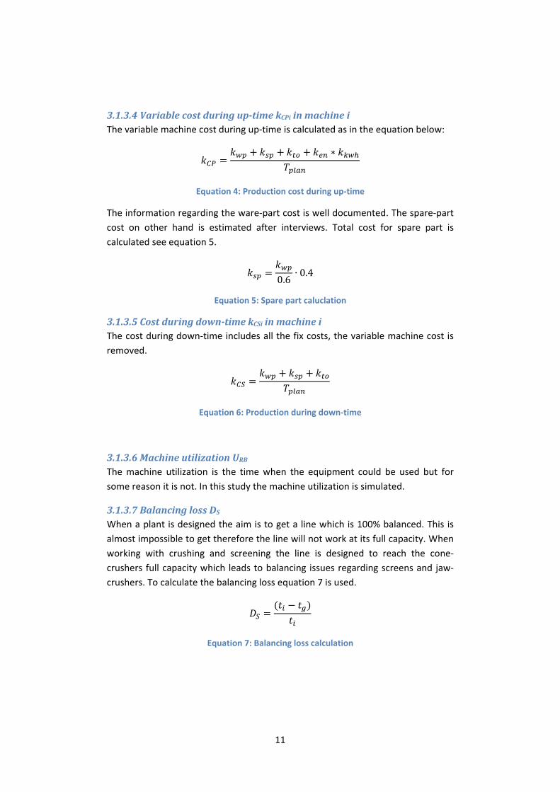
3.1.3.4Variablecostduringup‐timekCPiinmachineiThe variable machine cost during up‐time is calculated as in the equation below:
∗
Equation 4: Production cost during up‐time
The information regarding the ware‐part cost is well documented. The spare‐part
cost on other hand is estimated after interviews. Total cost for spare part is
calculated see equation 5.
0.6∙ 0.4
Equation 5: Spare part caluclation
3.1.3.5Costduringdown‐timekCSiinmachineiThe cost during down‐time includes all the fix costs, the variable machine cost is
removed.
Equation 6: Production during down‐time
3.1.3.6MachineutilizationURBThe machine utilization is the time when the equipment could be used but for
some reason it is not. In this study the machine utilization is simulated.
3.1.3.7BalancinglossDSWhen a plant is designed the aim is to get a line which is 100% balanced. This is
almost impossible to get therefore the line will not work at its full capacity. When
working with crushing and screening the line is designed to reach the cone‐
crushers full capacity which leads to balancing issues regarding screens and jaw‐
crushers. To calculate the balancing loss equation 7 is used.
Equation 7: Balancing loss calculation
12
3.1.3.8Production‐ratelossqpThe production‐rate loss occurs when the cycle time has to be increased, for
example if the production has quality problems. This variable is simulated
throughout this study.
3.1.3.9Down‐timerateqSThe true production time tp is longer than the nominal cycle time t0 because of
disturbances that result in downtime. In the crushing and screening process this
can be caused of the raw material distribution which will differ a lot at the
beginning to the end. By adding a downtime rate will deal with this problem.
3.1.3.10PayrollcostKDThe payroll cost is the total cost for the payroll during one year and then it is
divided by the metric ton produced.
3.2BuildingofthenewAdoptedProductionCostModelinExcelThe most time consuming part of this study was to implement the model in excel.
Programing has to be tried out during the study, a lot of try and error testing has
been made. One of the major advantages with the program is that it can easily be
changed if the validation points in any direction.
3.2.1VisualBasicforApplicationsVisual Basic for Applications (VBA) is a programming language in Microsoft Excel.
It is often used for writing macros in Excel. The author has used VBA for building
the calculation program. This was the easiest way of making a user friendly
interface in Microsoft Excel, which was one of the main tasks during this study.
3.2.2InterfaceThe main goal of the interface is to give the user a good idea of what to fill in in
order to make the calculations. The simplicity of the worksheet and the knowhow
of Excel was the main reason for developing the program instead of using
MathCad. There is a certain way of filling in the form in order to make the
calculations which is presented in the user manual in appendix. This manual will
also describe how the simulations are made.
13
3.2.3OutputThe Out‐put shall be easy to overview and give the most relevant results at the
top. This is done by putting the major cost groups at the top and then adding
these up to get the final production cost. This will give the user a good view of
what is included and what is the major cost driver that causes the production
cost. If the user has a good idea of what the production cost shall be then the
output worksheet can visualize if the user have done something wrong through
the calculations. There is also a script written to get the top ten cost drivers which
could be very efficient when using the program on a very large site.
3.2.5UserManualThe user manual is supposed to make the calculations easy to make when using
the program.
First of all the macro has to be enabling in Microsoft excel.
3.2.5.1InputVariablesPartIThe first step is to fill in the input variables in part – I.

14
Figure 3: The interface of the developed program
1. The turquoise cells are costs which the user has to fill in in order to make
the calculations.
2. The green cells will sum up when the turquoise once are correct filled in.
3. The dark blue overhead cost is optional if the cost is known.
4. The pink cell is used when the deprecation cost is calculated linier.
5. The dark pink cells are used when the deprecation cost takes the annuity
in to account.
6. The Yield is the fraction in percent of each produced product at the end.
3.2.5.2InputVariablesPartIIThe second part is to fill in the input variables in part II. If all the costs are known
the calculations are rather easy. For simulation read 3.2.5.3 Simulation Part III.
15
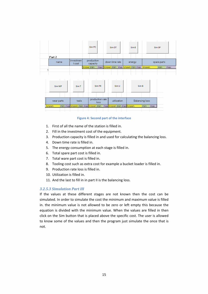
Figure 4: Second part of the interface
1. First of all the name of the station is filled in.
2. Fill in the investment cost of the equipment.
3. Production capacity is filled in and used for calculating the balancing loss.
4. Down time rate is filled in.
5. The energy consumption at each stage is filled in.
6. Total spare part cost is filled in.
7. Total ware part cost is filled in.
8. Tooling cost such as extra cost for example a bucket loader is filled in.
9. Production rate loss is filled in.
10. Utilization is filled in.
11. And the last to fill in in part II is the balancing loss.
3.2.5.3SimulationPartIIIIf the values at these different stages are not known then the cost can be
simulated. In order to simulate the cost the minimum and maximum value is filled
in. the minimum value is not allowed to be zero or left empty this because the
equation is divided with the minimum value. When the values are filled in then
click on the Sim button that is placed above the specific cost. The user is allowed
to know some of the values and then the program just simulate the once that is
not.
16
3.2.5.4RunFunctionWhen the entire chart is filled in the calculations can be made by clicking the Run
button.
3.2.5.5OutputVariablesPartIThe first part of the output shows the total cost per product where six different
costs are displayed.
1. Raw material
2. Labor cost fixed (over‐head cost)
3. Conveyor cost
4. Rental cost (land)
5. Total production cost
6. Total cost per product
3.2.5.6OutputVariablesPartIIThe second part of the output variables display how the production cost is
calculated and where the production costs occur. These costs are divided into four
different groups and when these are added up the total production cost is
displayed in the down right corner.
1. Deprecation
2. Production cost
3. Down time cost
4. Direct wages (payroll)
3.2.5.7Top‐TenCostDriversIn order to get the top ten cost drivers the user push the “Top Ten Cost” button
which then will pick out the ten major cost throughout the entire calculation
chart.
3.2.5.8EraseFunctionTo erase all values the user can either push the “Erase” button or just erase the
values manually.
3.2.4AssumptionsThere have been done some assumptions for this study:

17
1. The conveyor cost only depend on the deprecation cost this because of
the negligible cost for energy and maintenance cost.19
2. The spare part cost is calculated. The wear part cost is well known and
after interviews the common way of calculation the spare part cost is
shown in equation 5.
3. The simulated values are down time rate, production rate loss and
utilization.
4. The cost for setup is set to zero. The setup cost is in this study included in
the wear part cost because there is not any specific setup time when
producing the aggregate.
3.3Mont‐CarloSimulation20Monte‐Carlo Simulation (MCS) is most famous when it was used during the
Manhattan Project. It is often used when regular solving tools cannot be used21.
Ståhl describes how MCS can be used when there is a lack of historical data and
series, qualified assumptions need to serve as the basis for describing the
parameters in question in statistical terms. The most common distributions used
are Normal distribution or Weibull distribution. To get the right distributions
function at least two out of the five following questions has to be answered.
A – Is the frequency function symmetric or asymmetric?
B – What value does the most frequency occurring result for the parameter in
question have?
C – What is the lowest value for the parameter in question which is found to occur
have?
D – What is the highest value for the parameter in question which is found to
occur?
E – What is the average value obtained for the parameter in question?
The easiness of answering question C and D made Weibull distribution most
applicable for the program.
19 Interview: Manouchehri, Hamid, 2015 20 Development of Manufacturing Systems, 2013 21 Introduction of Monte Carlo simulation, 2010

18
4Results
This chapter will present the results from the calculations during this study. It will
also compare the results to the earlier study made by Lindström and Heyman.
Figure 6: The results from the production cost calculations
nameDeprecication production cost
Down time
cost
Direct
wages
sikt SW1252H 0,124772826 1,506399466 0,247678 0,57256502
käftkross CJ412 0,47719391 0,834388786 0,150046157 0,7491339
sikt SS1223H 0,110150152 1,030694371 0,169463895 0,34584353
Konkross CS440 0,391597969 3,337636494 0,630193859 1,29099418
sikt MSO2060D 0,166675696 1,546041557 0,254195842 0,78497909
Konkross CH666 0,517782611 2,881264468 0,463907412 1,48345675
Konkross Vibro 1,427683977 1,605087968 0,29055997 2,24128272
Sikt MSO2160S 0,127379464 0,837439177 0,137689415 0,3249506
Sikt MSO 2160S 0,127379464 0,966275973 0,158872401 0,374943
3,470616069 14,54522826 2,50260695 8,16814879 28,6866
Primary crushing
Secondary crushing
Tertiary crushing
Stockpile
Figure 5: Flow sheet over the production
19
Table 1: Total cost for production at the company according to this study
4.1
4.1.1RawmaterialcostThe raw material is taken from the early study made by Heyman and Lindström,it
is set to 15.25 SEK/ton
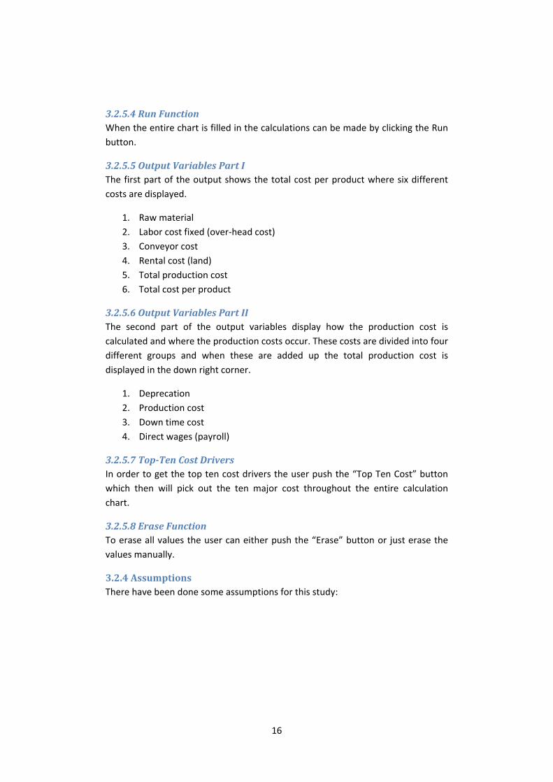
4.1.2PayrollcostThe payroll cost generated in this study is 8.27 SEK/ton and the previous result is
5.22 SEK/ton
Figure 7: Payroll distribution function according to Heyman and Lindström22
The payroll cost is one of the factors that has been changed to more accurate way
therefor the one and old results differ.
4.1.3MachinecostduringuptimeThe machine cost during uptime is 14.55 SEK/ton and the previous result is 24.16
SEK/ton
22 Cost Analysis for Crushing and Screening – Part I, 2014
raw material Labour cost fixed Conveyor Cost Rental Cost
Total
productio
n Cost
Total Cost
15,248 0 0,533333333 3,33333333 28,6866 47,801267
2 3.5 5 6.5 80
0.2
0.4
0.6
0.8
1S[-]
kDmean
[SEK/ton]
20
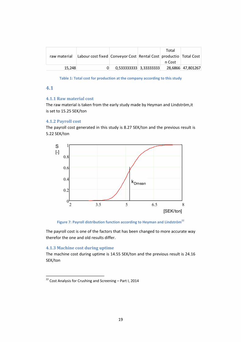
Figure 8: Distribution function over production cost during up‐time according to Heyman and Lindström23
This result is not so surprising since the deprecation cost is not included in the
production cost in the new calculation. When adding the deprecation cost to the
production cost the result is 18.00 SEK/ton with liner deprecation. In previous
study the deprecation cost is calculated with annuity and by using a residual value
this affect the total machine cost during uptime.
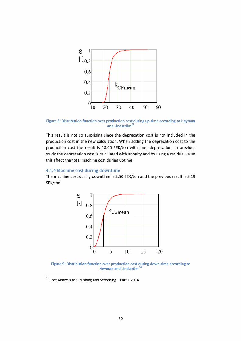
4.1.4MachinecostduringdowntimeThe machine cost during downtime is 2.50 SEK/ton and the previous result is 3.19
SEK/ton
Figure 9: Distribution function over production cost during down‐time according to Heyman and Lindström 24
23 Cost Analysis for Crushing and Screening – Part I, 2014
10 20 30 40 50 600
0.2
0.4
0.6
0.8
1S[-]
kCPmean
0 5 10 15 200
0.2
0.4
0.6
0.8
1S[-]
kCSmean

21
In this case the new calculation is placed well in the distribution function. The
difference in this case can once again depend on the fact that the deprecation
cost not is included in the sum of the production cost.
4.1.5TotalproductioncostpermetrictonThe total cost is hard to compare when they differences between them is rather
large when it comes to payroll cost and deprecation cost. There is also a rather
large difference in the rental cost according to new input. When comparing the
production costs, without payroll and deprecation cost. This study gave the result
of 36.16 SEK/ton and the previous study gave the result of 31.93 SEK/ton. This
study has a rental cost that is 3.33 SEK/ton and the previous one only calculated
with 0.2 SEK/ton. With that removed the cost would have been 32.82 SEK/ton
compared to 31.73 SEK/ton. This is well in the 85% accuracy that this study aimed
for.
4.2Resultanalysis
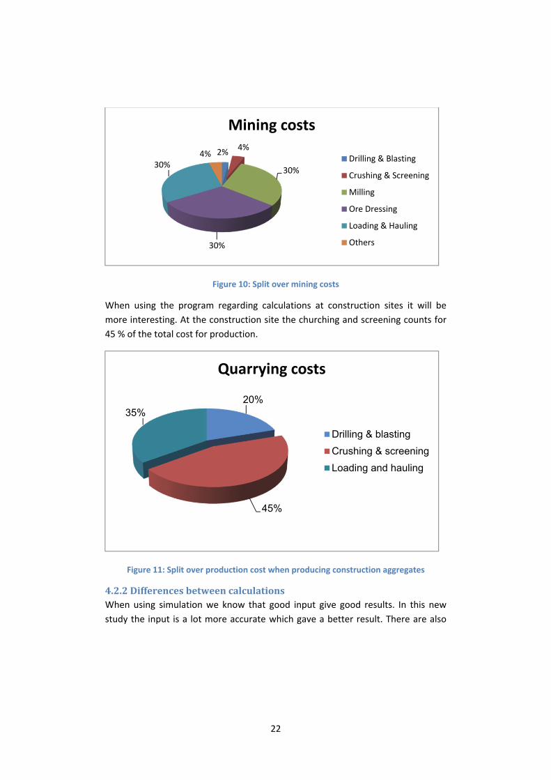
4.2.1TotalproductioncostThe total production cost does not differ substantially. In this study less
parameters has been simulated then in the previous study and instead the
parameters were estimated by persons with good insight in the crushing and
screening process. This result is in line with the Mining Cost in diagram25.. The cost
of crushing and screening is 2/3 and the raw material is 1/3. This study gave the
result of 47.80 SEK/ton where raw material is 15.25 SEK/ton.
24 Cost Analysis for Crushing and Screening – Part I, 2014 25 Sandvik Rock Processing Manual, 2011
22
Figure 10: Split over mining costs
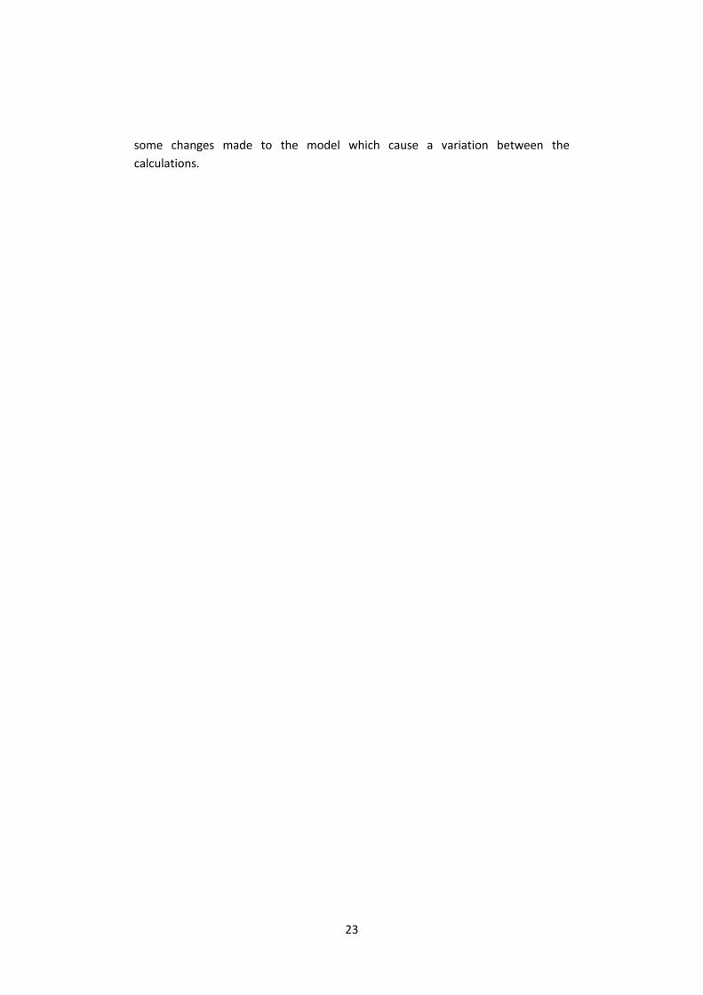
When using the program regarding calculations at construction sites it will be
more interesting. At the construction site the churching and screening counts for
45 % of the total cost for production.
Figure 11: Split over production cost when producing construction aggregates
4.2.2DifferencesbetweencalculationsWhen using simulation we know that good input give good results. In this new
study the input is a lot more accurate which gave a better result. There are also
2%4%
30%
30%
30%4%
Mining costs
Drilling & Blasting
Crushing & Screening
Milling
Ore Dressing
Loading & Hauling
Others
20%
45%
35%
Quarrying costs
Drilling & blasting
Crushing & screening
Loading and hauling
23
some changes made to the model which cause a variation between the
calculations.

24
5ConclusionsThe program seems to give a rather precise value of the total production cost. The
differences between this study and Heyman and Lindstöms result are due to fact
that payroll cost and deprecation cost are calculated in a different way. The major
problem is that the validation of the calculation could not be done because lack of
sites willing to investigate their production cost.
In this study the ware part cost was well known which made the study more
accurate than the previous one. This also caused the production cost to decrease
but the payroll cost increased which made the total production cost to be at the
same level.
The aim of reaching 85 % accuracy was even better than expected but without
further validations this result cannot be seen as significant a quantitative study
would prove this.
This result might show that a higher level of atomization could be preferred in a
county as Sweden when the payroll cost has such a high impact on the result.
In this study there have still been many input variables which cause the
calculations to be a little bit time consuming.
25
6FurtherstudiesThe most important study that can be done is to validate the program by a
quantitative study. This might show that a beta parameter have to be added to
the calculation. The beta parameter is a value which can reduce volatility if there
is cost that is not included in the program for example the small amount of dust
which disappears when crushing. It would be interesting to see if the assumptions
throughout this study are right. If so then the study could be done by just knowing
very few input variables.
It would be interesting to study the connection between work index or abrasion
index and the wear part cost, than the simulations could be done by greater
accuracy.
Building a simulation program is an ongoing process which can always be
improved. When the validation is made there could be some adjustments to the
program which might give a more detailed result.

26
6References
LiteratureBergman, Kjell. (2007). ”Gjuteritet 125 år – En Kulturhistoria”. Wallin & Dalholm
Boktryckeri AB, Lund.
Höst, Martin, Regnell, Björn och Runesson, Per. (2006). Att genomföra
examensarbete. Studentlitteratur, Lund.
Ståhl, Jan‐Eric. (2010). Industriella Tillverkningssystem del II – Länken mellan
teknink och ekonomi. 2 uppl. Industriell produktion LTH, Lunds Universitet.
Ståhl, Jan‐Eric. (2013). Development of Manufacturing Systems – The link
between technology and economics. 1 uppl. Industriell produktion LTH, Lunds
Universitet.
Sandvik Årsredovisning 2014.
Lekwall, Per, Wahlbin, Clas. (2001). Information för marknadsföringsbeslut. 4
uppl. IHM Publishing, Göteborg.
Björklund, Maria, Paulsson. (2003). Seminarieboken – att skriva, presentera och
opponera. Studedentlitteratur, Lund
Lindström, Alexander, Heyman R, Erik. (2014). Cost Analysis for Crushing and
Screening – Part I. Division of Production and Materials Engineering, Lund
University.
Sandvik Rock Processing Manual. Svedala, Sandvik. (2013).
ArticlesLaw, Averill M, McComas, Michael G. (2001). How to bulid and credible simulation
models. Proceedings of the 2001 Winter Simulation Conference, B. A. Peters, J.S.
Smith, D. J. Medeiros, and M. W. Rohrer, eds.
Harrison, Robert L. (2010). Introduction To Monte Carlo Simulation. AIP Conf Proc.
27
ElectronicresourcesSandvik.se
Sandvik Mining and Construction intranät Sverige.
InterviewsHedvall, Per. Senior Advisor (continously).
Paravac, Marijan. Market & Sales Manager (continously).
Svedensten, Per. Manager Crushing Chambers and Material Development
(continuously)
Manouchehri, Hamid. Principal Advisor Sandvik SRP (continuously)
Hanny, Steven.

28
Appendix
AppendixAAl Abression Index kg/kWh
C&S Crushing and Screening ‐
D Balancing loss for station ‐
HIS High Speed Impact ‐
K Production cost of prduct SEK/ton
K0 Original investment of equipment SEK
kB Cost of raw material SEK/ton
kCP Machine cost during up‐time SEK/ton
kCS Machine cost during down‐time SEK/ton
KD Payroll cost SEK/ton
ken Energy consumption kW/h
kkwh Cost per kWh SEK/kWh
ksp Spare part cost SEK/year
kto Tooling cost SEK/year
kwp Wear part cost SEK/year
PD Plant Designer ‐
PF Production factor at end of process %
qP Production rate loss ‐
qS Downtime rate ‐
Tplan Planned production time per year hours
TSU Set‐up time hours

29
URP Machine utilization ‐
VSI Vertical Shaft Impact ‐
Y Yield %
AppendixB(HeymanandLindströmindex)
af Annuity ‐
AI Abrasion Index kg/kWh
C&S Crushing & Screening ‐
CSS Close Side Setting mm
D Balancing loss for station ‐
F80 The 80 % passing size of the feed µm
HIS High Speed Impact ‐
hUH Number of hours of operation per hour maintenance ‐
hy Number of hours per shift per year hours/year
k Production cost of product SEK/part
K0 Original investment of equipment SEK
kB Cost of raw material per ton SEK/ton
kCP Hourly cost of machine during production SEK/hour
kCS Hourly cost of machine during downtime and setup times
SEK/hour
kD Payroll costs SEK/hour
kph Variable machine time cost SEK/hour
kren Average renovation cost SEK
krenk Renovation cost SEK
kUHh Maintenance cost per hour SEK/hour
ky Cost per square meter SEK/m2
lön Average salary SEK/year
30
M Tons of raw material used for 1 ton of main product tons
M0 1 ton of main product at end of process ton
mf Material flow ton/hour
MIT Massachusetts Institute of Technology ‐
MLOC Machine Lifetime Operating Cost ‐
n Expected length of time in use year
N0 Batch size number
nop Number personnel connected to the production line
number
Nren Number of renovations during lifetime ‐
Nren Number of renovations number
nren Year of renovation, from present time years
nsyren Number of shift‐yeas between renovations years
OFAT One Factor At Time ‐
p Internal rate ‐
P80 The 80 % passing size of the ground product µm
PD PlantDesigner ‐
PF Product factor at end of process ‐
pf Product factor for station and product ‐
PPM Production Performance Matrix ‐
PTC Parametric Technology Company ‐
qB Rejection rate ‐
qP Production‐rate loss ‐
qS Downtime rate ‐
r% Residual value ‐
ra Residual value factor ‐
socavg Social security costs ‐
SPS Swedish Production Symposium ‐
t0 Cycle time min/part
Tfree Free capacity hours

31
tmf Time to process 1 ton of material hour/ton
Tplan Planned production time per year hours
Tsu Setup time for machine hours
URP Machine utilization ‐
VSI Vertical Shaft Impact ‐
W Work Impact Index kWh/ton
Wi Bond work index kWh/ton
Yky Cost for the C&S plant or facility in terms of rent or depreciations
m2
Recommended