CPU Scheduling
Properties of Processes
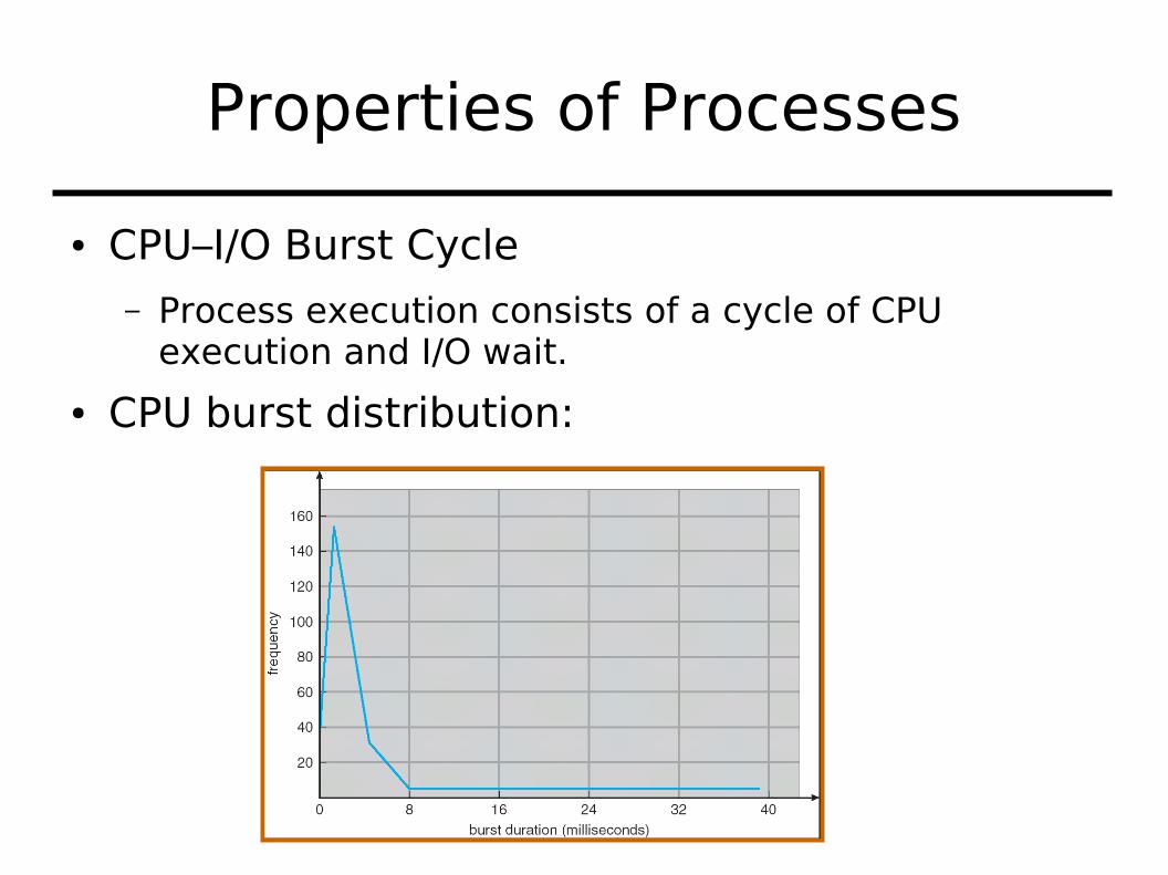
● CPU–I/O Burst Cycle– Process execution consists of a cycle of CPU
execution and I/O wait.
● CPU burst distribution:
CPU Scheduler
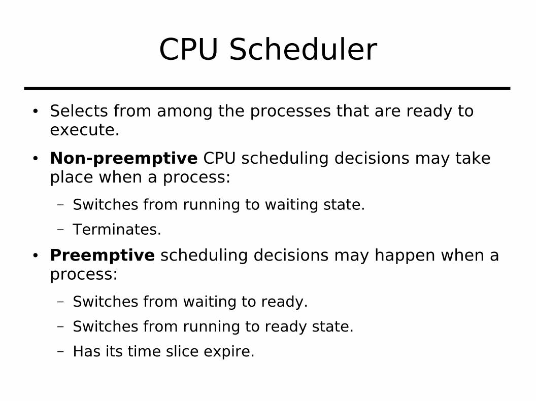
● Selects from among the processes that are ready to execute.
● Non-preemptive CPU scheduling decisions may take place when a process:
– Switches from running to waiting state.
– Terminates.
● Preemptive scheduling decisions may happen when a process:
– Switches from waiting to ready.
– Switches from running to ready state.
– Has its time slice expire.
Dispatcher
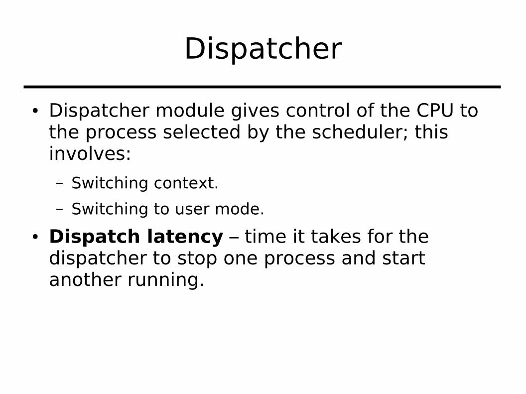
● Dispatcher module gives control of the CPU to the process selected by the scheduler; this involves:– Switching context.
– Switching to user mode.
● Dispatch latency – time it takes for the dispatcher to stop one process and start another running.
Scheduling Criteria
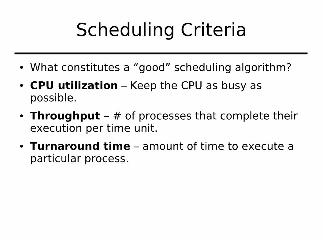
● What constitutes a “good” scheduling algorithm?
● CPU utilization – Keep the CPU as busy as possible.
● Throughput – # of processes that complete their execution per time unit.
● Turnaround time – amount of time to execute a particular process.
Scheduling Criteria
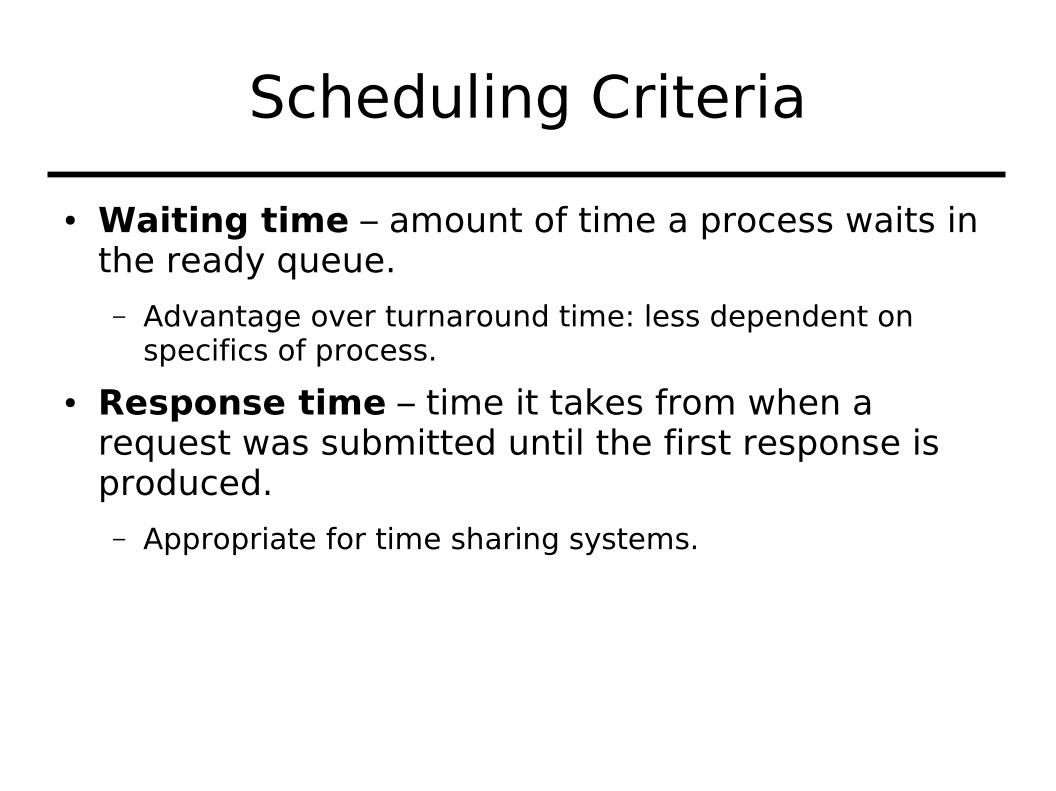
● Waiting time – amount of time a process waits in the ready queue.
– Advantage over turnaround time: less dependent on specifics of process.
● Response time – time it takes from when a request was submitted until the first response is produced.
– Appropriate for time sharing systems.
First Come First Serve Scheduling (FCFS)
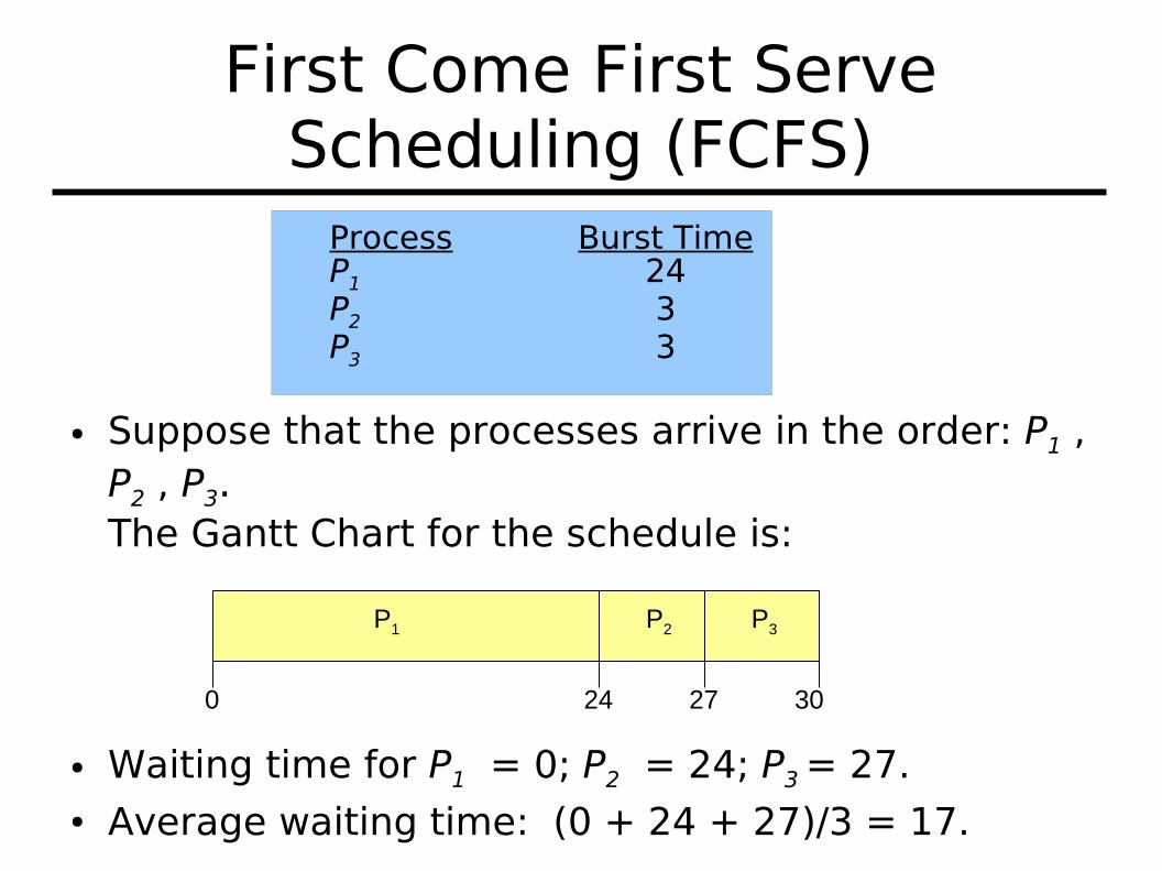
● Suppose that the processes arrive in the order: P1 , P2 , P3. The Gantt Chart for the schedule is:
● Waiting time for P1 = 0; P2 = 24; P3 = 27.● Average waiting time: (0 + 24 + 27)/3 = 17.
P1 P2 P3
24 27 300
Process Burst TimeP1 24P2 3P3 3
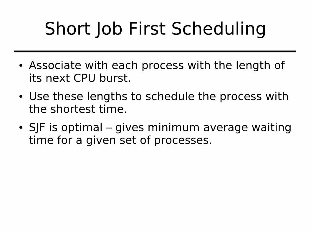
Short Job First Scheduling
● Associate with each process with the length of its next CPU burst.
● Use these lengths to schedule the process with the shortest time.
● SJF is optimal – gives minimum average waiting time for a given set of processes.
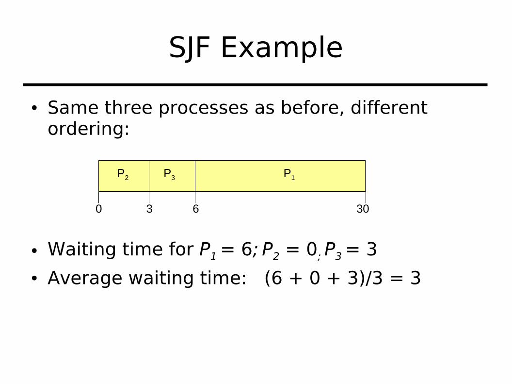
SJF Example
● Same three processes as before, different ordering:
● Waiting time for P1 = 6; P2 = 0; P3 = 3● Average waiting time: (6 + 0 + 3)/3 = 3
P1P3P2
63 300
SJF Variants
● Non-preemptive – once CPU given to the process it cannot be preempted until completes its CPU burst
● Preemptive – if a new process arrives with CPU burst length less than remaining time of current executing process, preempt. This scheme is know as the Shortest-Remaining-Time-First (SRTF)
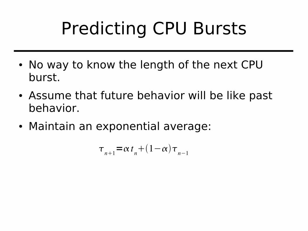
Predicting CPU Bursts
● No way to know the length of the next CPU burst.
● Assume that future behavior will be like past behavior.
● Maintain an exponential average:
n1
= tn1−
n−1
Priority Scheduling
● A priority number (integer) is associated with each process.
● The CPU is allocated to the process with the highest priority (smallest integer = highest priority.)– Preemptive.
– Non-preemptive.
● Problem: starvation – low priority processes may never execute.
● Solution: aging – as time progresses increase the priority of the process.
Round Robin
● Each process gets a small quantum, usually 10-100 milliseconds.
● After this time has elapsed, the process is preempted and added to the end of the ready queue.
● If there are n processes in the ready queue and the time quantum is q, then each process gets 1/n of the CPU time in chunks of at most q time units at once.
● No process waits more than (n-1)q time units.
Round Robin Performance
● q large ->FIFO
● q small -> q must be large with respect to context switch, otherwise overhead is too high
● In general, RR has higher turnaround time than SJF, but better response time.
Multi-level Queue
● Ready queue is partitioned into separate queues. For example:– foreground (interactive)
– background (batch)
● Each queue has its own scheduling algorithm– foreground – RR
– background – FCFS
● Can maintain responsiveness in the face of CPU bound tasks.
Multi-level Queue
● Scheduling must be done between the queues
● Fixed priority scheduling; (i.e., serve all from foreground then from background). – Possibility of starvation.
● Time slice – each queue gets a certain amount of CPU time which it can schedule amongst its processes, e.g.:– 80% to foreground in RR
– 20% to background in FCFS
Multi-level Feedback Queue
● A process can move between the various queues.– Aging can be implemented this way.
– Processes can be organized according to their CPU burstiness.
– I/O bound processes will end up in higher level queues.
● (Some of the same goals can be met with dynamic priority based schemes. – Processes get priority boosts based on being I/O
bound.)
Multi-level Feedback Queue
● Multilevel-feedback-queue scheduler defined by the following parameters:– Number of queues.
– Scheduling algorithms for each queue.
– Method used to determine when to upgrade a process.
– Method used to determine when to demote a process.
– Method used to determine which queue a process will enter when that process needs service.
Multi-processor Scheduling
● Some new issues arise:– Processor affinity.
– Load balancing.● Push vs. Pull migration.
– Hyperthreading aware scheduling.
Real Time Scheduling
● Hard real-time systems – required to complete a critical task within a guaranteed amount of time.– Challenging to implement.
● Soft real-time systems – requires that critical processes receive priority over less fortunate ones.– Just requires a mechanism for very high priority
processes.
Thread Scheduling
● Process contention scope (PCS):– Library scheduling of threads within a process.
● System contention scope (SCS):– Scheduling of kernel threads.
Algorithm Evaluation
● Develop some model of the computer system and scheduler.– “Model” may be a complete implementation.
– “Model” may be an abstract description of the scheduling algorithm: “RR”.
● See how the model performs on sample input.– Simple description of a set of jobs.
– Trace information from a running system.
– Data generated from probability distributions.
Acknowledgments
● Portions of these slides are taken from Power Point presentations made available along with:– Silberschatz, Galvin, and Gagne. Operating System
Concepts, Seventh Edition.
● Original versions of those presentations can be found at:– http://os-book.com/
Recommended