D – 1
Operations ManagementOperations ManagementModule D – Waiting-Line ModelsModule D – Waiting-Line Models
© 2006 Prentice Hall, Inc.
PowerPoint presentation to accompanyPowerPoint presentation to accompany Heizer/Render Heizer/Render Principles of Operations Management, 6ePrinciples of Operations Management, 6eOperations Management, 8e Operations Management, 8e
D – 2
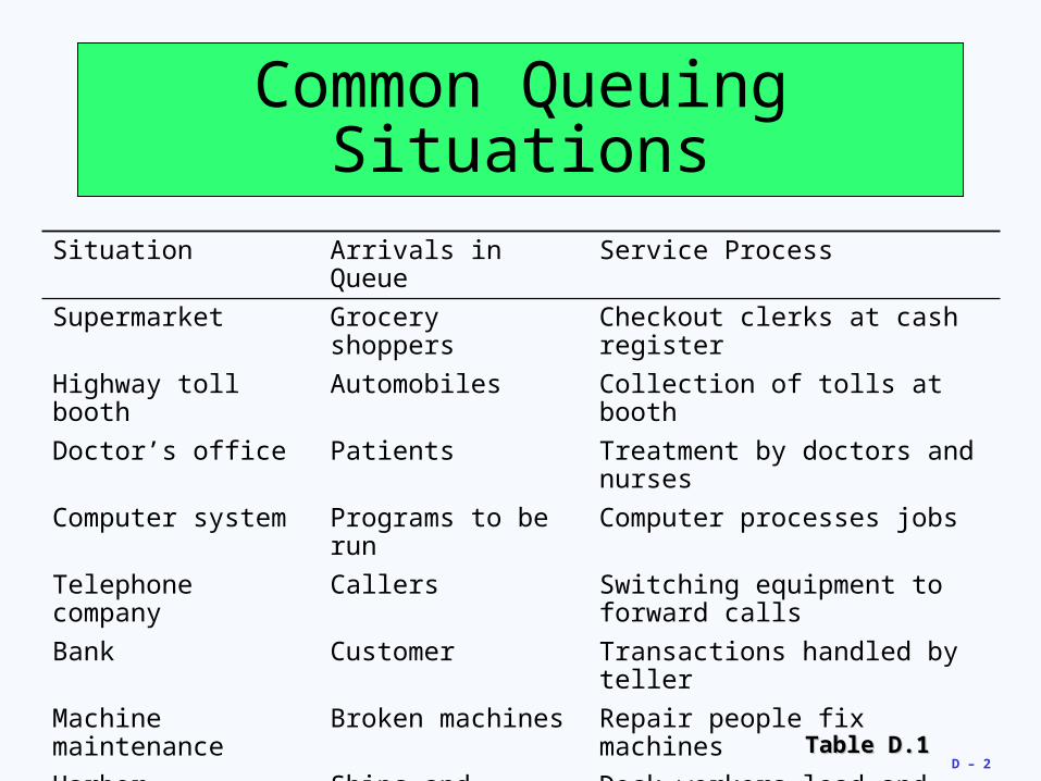
Common Queuing Situations
Situation Arrivals in Queue Service Process
Supermarket Grocery shoppers Checkout clerks at cash register
Highway toll booth Automobiles Collection of tolls at booth
Doctor’s office Patients Treatment by doctors and nurses
Computer system Programs to be run Computer processes jobs
Telephone company Callers Switching equipment to forward calls
Bank Customer Transactions handled by teller
Machine maintenance Broken machines Repair people fix machines
Harbor Ships and barges Dock workers load and unload
Table D.1Table D.1
D – 3
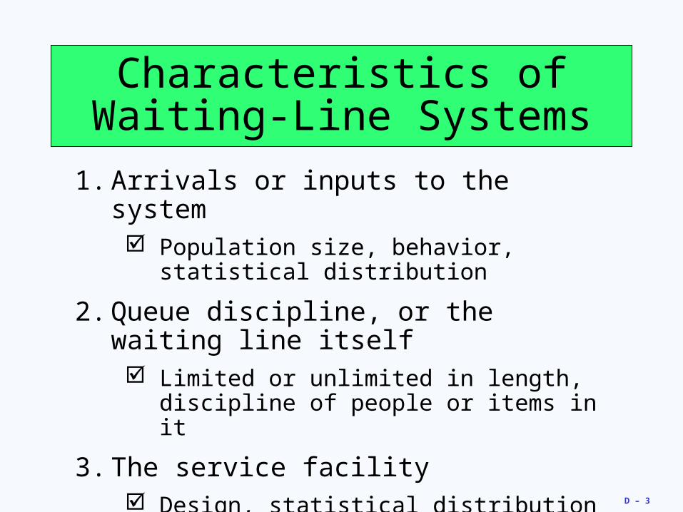
Characteristics of Waiting-Line Systems
1. Arrivals or inputs to the system Population size, behavior, statistical
distribution
2. Queue discipline, or the waiting line itself Limited or unlimited in length, discipline of
people or items in it
3. The service facility Design, statistical distribution of service
times
D – 4
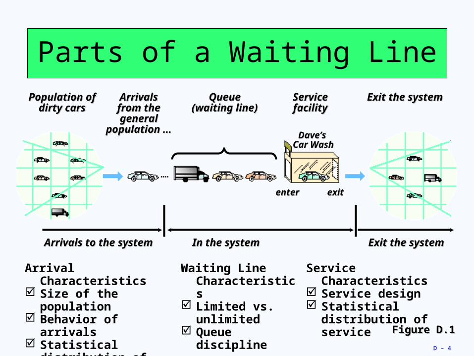
Parts of a Waiting Line
Figure D.1Figure D.1
Dave’s Dave’s Car WashCar Wash
enterenter exitexit
Population ofPopulation ofdirty carsdirty cars
ArrivalsArrivalsfrom thefrom thegeneralgeneral
population …population …
QueueQueue(waiting line)(waiting line)
ServiceServicefacilityfacility
Exit the systemExit the system
Arrivals to the systemArrivals to the system Exit the systemExit the systemIn the systemIn the system
Arrival Characteristics Size of the population Behavior of arrivals Statistical distribution
of arrivals
Waiting Line Characteristics
Limited vs. unlimited
Queue discipline
Service Characteristics Service design Statistical distribution
of service
D – 5
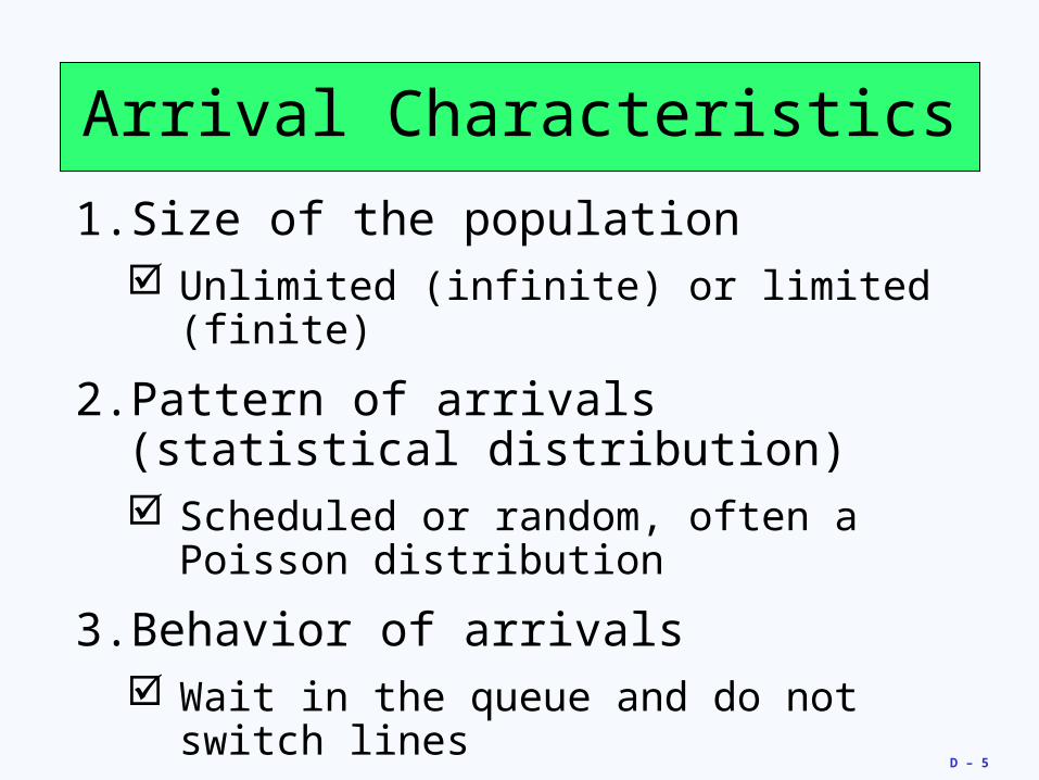
Arrival Characteristics
1. Size of the population Unlimited (infinite) or limited (finite)
2. Pattern of arrivals (statistical distribution) Scheduled or random, often a Poisson
distribution
3. Behavior of arrivals Wait in the queue and do not switch lines
Balking or reneging
D – 6
Poisson Distribution
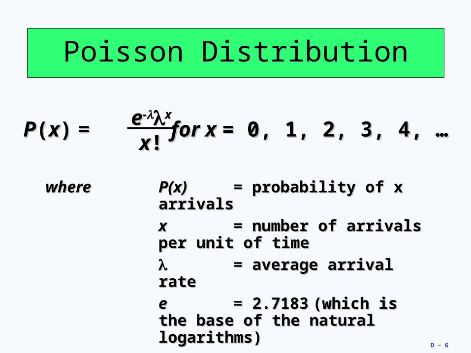
PP((xx)) = for x = for x = 0, 1, 2, 3, 4, …= 0, 1, 2, 3, 4, …ee--xx
xx!!
wherewhere P(x)P(x) == probability of x arrivalsprobability of x arrivals
xx == number of arrivals per number of arrivals per unit of timeunit of time
== average arrival rateaverage arrival rate
ee == 2.71832.7183 (which is the (which is the base of the natural logarithms)base of the natural logarithms)
D – 7
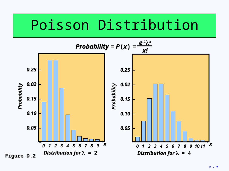
Poisson DistributionProbability = PProbability = P((xx)) = =
ee--xx
x!x!
0.25 0.25 –
0.02 0.02 –
0.15 0.15 –
0.10 0.10 –
0.05 0.05 –
–
Pro
bab
ility
Pro
bab
ility
00 11 22 33 44 55 66 77 88 99
Distribution for Distribution for = 2 = 2
xx
0.25 0.25 –
0.02 0.02 –
0.15 0.15 –
0.10 0.10 –
0.05 0.05 –
–
Pro
bab
ility
Pro
bab
ility
00 11 22 33 44 55 66 77 88 99
Distribution for Distribution for = 4 = 4
xx1010 1111
Figure D.2Figure D.2
D – 8
Waiting-Line Characteristics
Limited or unlimited queue length
Queue discipline: first-in, first-out is most common
Other priority rules may be used in special circumstances
D – 9
Service Characteristics
Queuing system designs Single-channel system, multiple-channel
system
Single-phase system, multiphase system
Service time distribution Constant service time
Random service times, usually a negative exponential distribution
D – 10
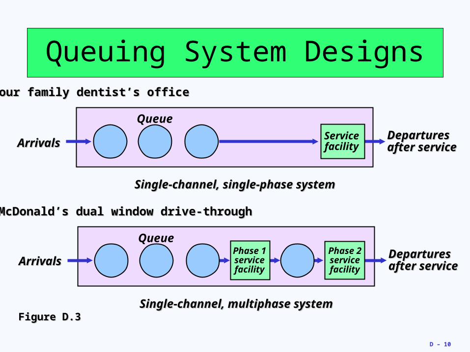
Queuing System Designs
Figure D.3Figure D.3
DeparturesDeparturesafter serviceafter service
Single-channel, single-phase systemSingle-channel, single-phase system
Queue
ArrivalsArrivals
Single-channel, multiphase systemSingle-channel, multiphase system
ArrivalsArrivalsDeparturesDeparturesafter serviceafter service
Phase 1 service facility
Phase 2 service facility
Service facility
Queue
Your family dentist’s officeYour family dentist’s office
McDonald’s dual window drive-throughMcDonald’s dual window drive-through
D – 11
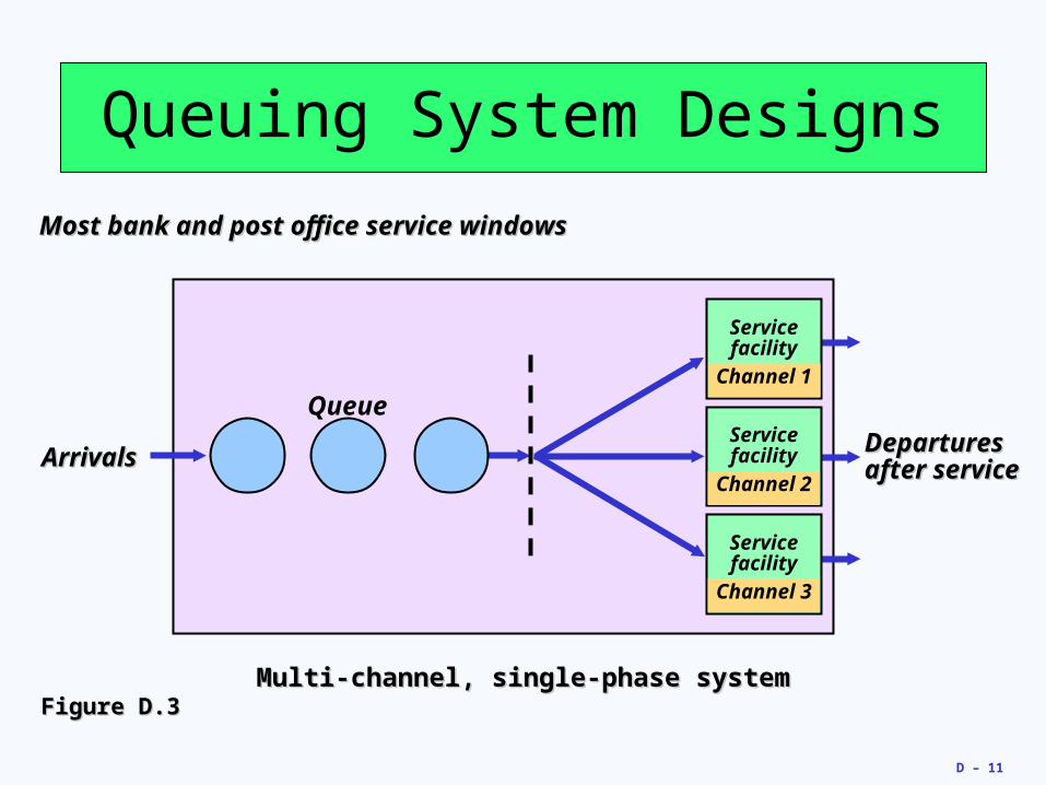
Queuing System Designs
Figure D.3Figure D.3Multi-channel, single-phase systemMulti-channel, single-phase system
ArrivalsArrivals
Queue
Most bank and post office service windowsMost bank and post office service windows
DeparturesDeparturesafter serviceafter service
Service facility
Channel 1
Service facility
Channel 2
Service facility
Channel 3
D – 12
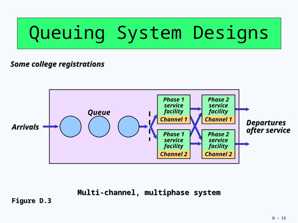
Queuing System Designs
Figure D.3Figure D.3Multi-channel, multiphase systemMulti-channel, multiphase system
ArrivalsArrivals
Queue
Some college registrationsSome college registrations
DeparturesDeparturesafter serviceafter service
Phase 2 service facility
Channel 1
Phase 2 service facility
Channel 2
Phase 1 service facility
Channel 1
Phase 1 service facility
Channel 2
D – 13
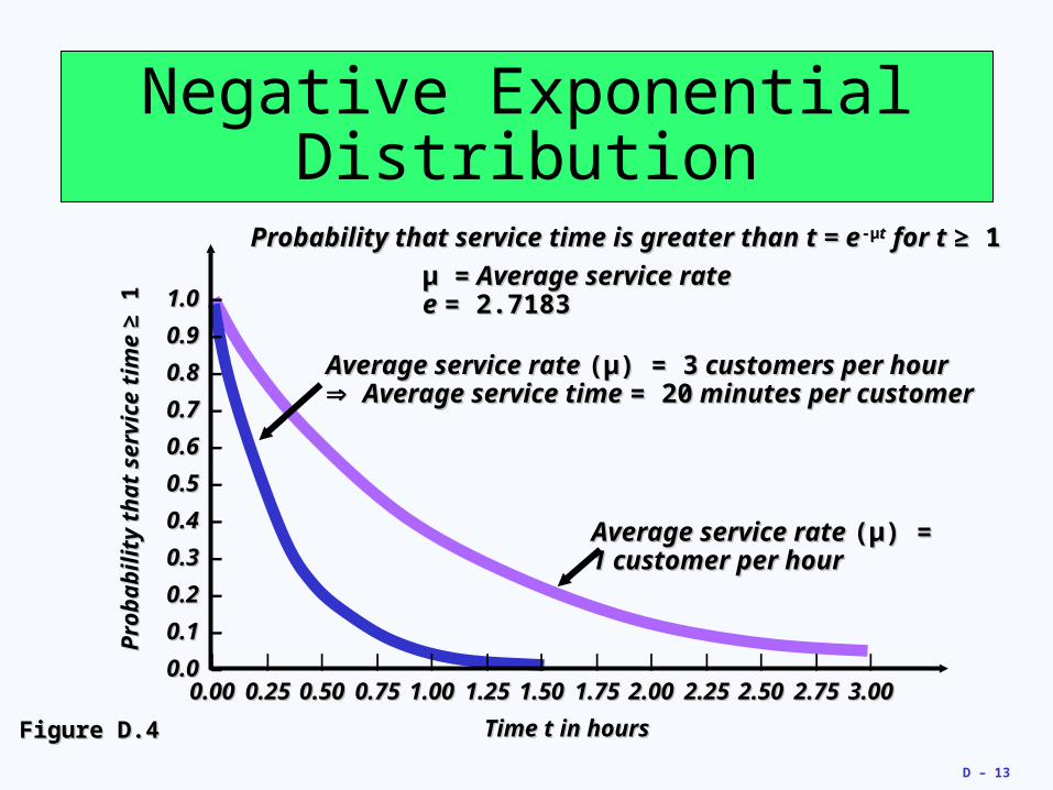
Negative Exponential Distribution
Figure D.4Figure D.4
1.0 1.0 –
0.9 0.9 –
0.8 0.8 –
0.7 0.7 –
0.6 0.6 –
0.5 0.5 –
0.4 0.4 –
0.3 0.3 –
0.2 0.2 –
0.1 0.1 –
0.0 0.0 –
Pro
bab
ility
th
at s
ervi
ce t
ime
Pro
bab
ility
th
at s
ervi
ce t
ime
≥ 1
≥ 1
| | | | | | | | | | | | |
0.000.00 0.250.25 0.500.50 0.750.75 1.001.00 1.251.25 1.501.50 1.751.75 2.002.00 2.252.25 2.502.50 2.752.75 3.003.00
Time t in hoursTime t in hours
Probability that service time is greater than t = eProbability that service time is greater than t = e-µ-µtt for t for t ≥ 1≥ 1
µ =µ = Average service rate Average service ratee e = 2.7183= 2.7183
Average service rate Average service rate (µ) = (µ) = 1 customer per hour1 customer per hour
Average service rate Average service rate (µ) = 3(µ) = 3 customers per hour customers per hour Average service time Average service time = 20= 20 minutes per customer minutes per customer

D – 14
Measuring Queue Performance
1. Average time that each customer or object spends in the queue
2. Average queue length
3. Average time in the system
4. Average number of customers in the system
5. Probability the service facility will be idle
6. Utilization factor for the system
7. Probability of a specified number of customers in the system
D – 15
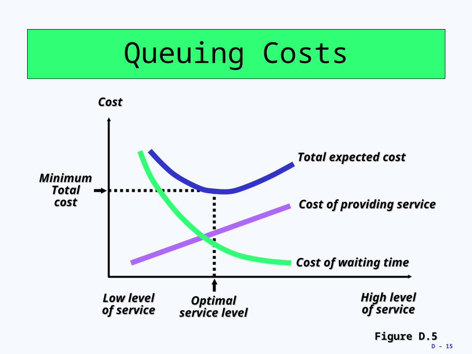
Queuing Costs
Figure D.5Figure D.5
Total expected costTotal expected cost
Cost of providing serviceCost of providing service
CostCost
Low levelLow levelof serviceof service
High levelHigh levelof serviceof service
Cost of waiting timeCost of waiting time
MinimumMinimumTotalTotalcostcost
OptimalOptimalservice levelservice level
D – 16
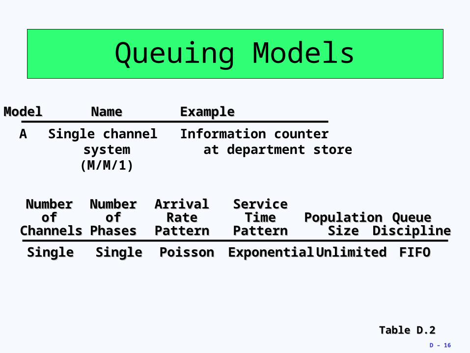
Queuing Models
Table D.2Table D.2
ModelModel NameName ExampleExample
A Single channel Information counter system at department store(M/M/1)
NumberNumber NumberNumber ArrivalArrival ServiceServiceofof ofof RateRate TimeTime PopulationPopulation QueueQueue
ChannelsChannels PhasesPhases PatternPattern PatternPattern SizeSize DisciplineDiscipline
SingleSingle SingleSingle PoissonPoisson ExponentialExponential UnlimitedUnlimited FIFOFIFO
D – 17
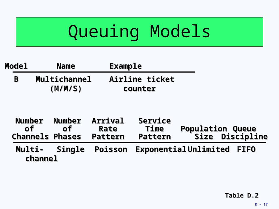
Queuing Models
Table D.2Table D.2
ModelModel NameName ExampleExample
BB Multichannel Multichannel Airline ticketAirline ticket (M/M/S) (M/M/S) counter counter
NumberNumber NumberNumber ArrivalArrival ServiceServiceofof ofof RateRate TimeTime PopulationPopulation QueueQueue
ChannelsChannels PhasesPhases PatternPattern PatternPattern SizeSize DisciplineDiscipline
Multi-Multi- SingleSingle PoissonPoisson ExponentialExponential UnlimitedUnlimited FIFOFIFO channelchannel

D – 18
Queuing Models
Table D.2Table D.2
ModelModel NameName ExampleExample
CC Constant Constant Automated car Automated car service service wash wash(M/D/1)(M/D/1)
NumberNumber NumberNumber ArrivalArrival ServiceServiceofof ofof RateRate TimeTime PopulationPopulation QueueQueue
ChannelsChannels PhasesPhases PatternPattern PatternPattern SizeSize DisciplineDiscipline
SingleSingle SingleSingle PoissonPoisson ConstantConstant UnlimitedUnlimited FIFOFIFO
D – 19
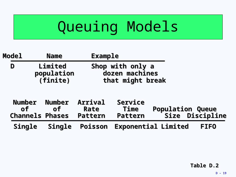
Queuing Models
Table D.2Table D.2
ModelModel NameName ExampleExample
DD Limited Limited Shop with only a Shop with only a population population dozen machines dozen machines
(finite)(finite) that might break that might break
NumberNumber NumberNumber ArrivalArrival ServiceServiceofof ofof RateRate TimeTime PopulationPopulation QueueQueue
ChannelsChannels PhasesPhases PatternPattern PatternPattern SizeSize DisciplineDiscipline
SingleSingle SingleSingle PoissonPoisson ExponentialExponential LimitedLimited FIFOFIFO
D – 20
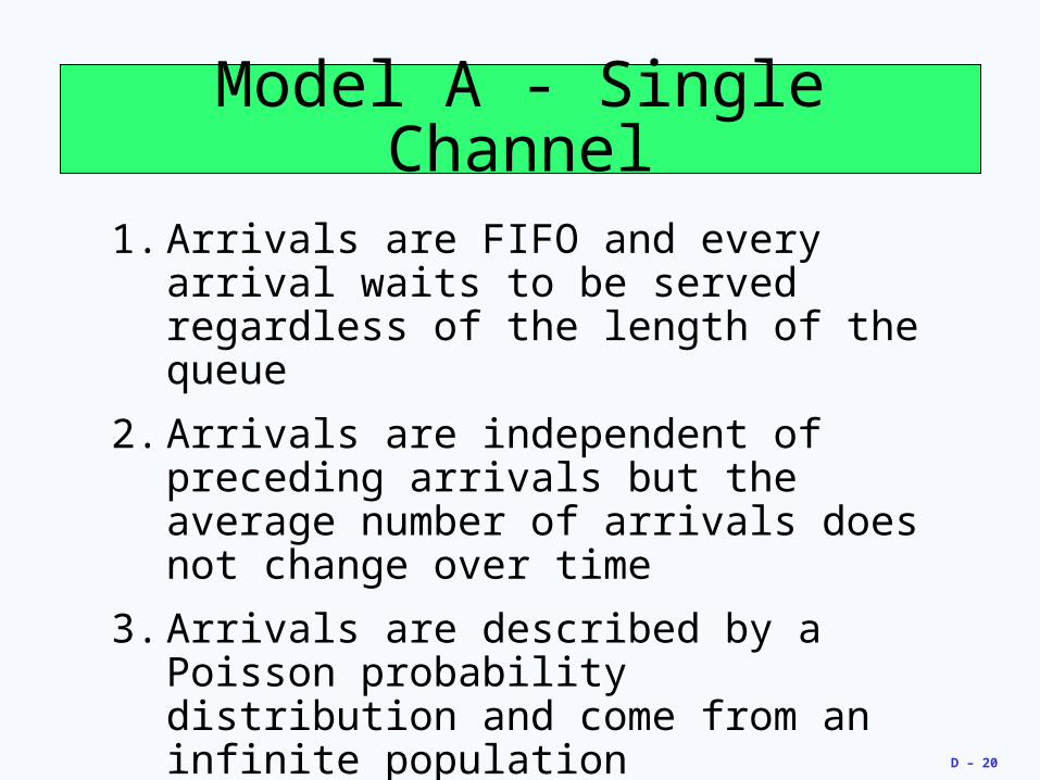
Model A - Single Channel
1. Arrivals are FIFO and every arrival waits to be served regardless of the length of the queue
2. Arrivals are independent of preceding arrivals but the average number of arrivals does not change over time
3. Arrivals are described by a Poisson probability distribution and come from an infinite population
D – 21
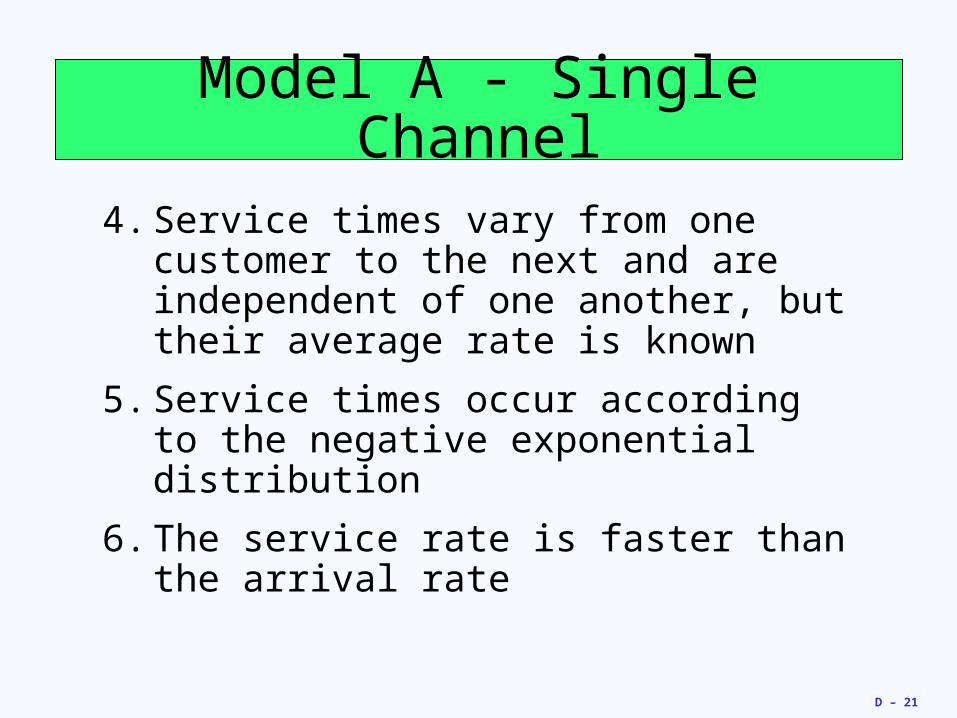
Model A - Single Channel
4. Service times vary from one customer to the next and are independent of one another, but their average rate is known
5. Service times occur according to the negative exponential distribution
6. The service rate is faster than the arrival rate
D – 22
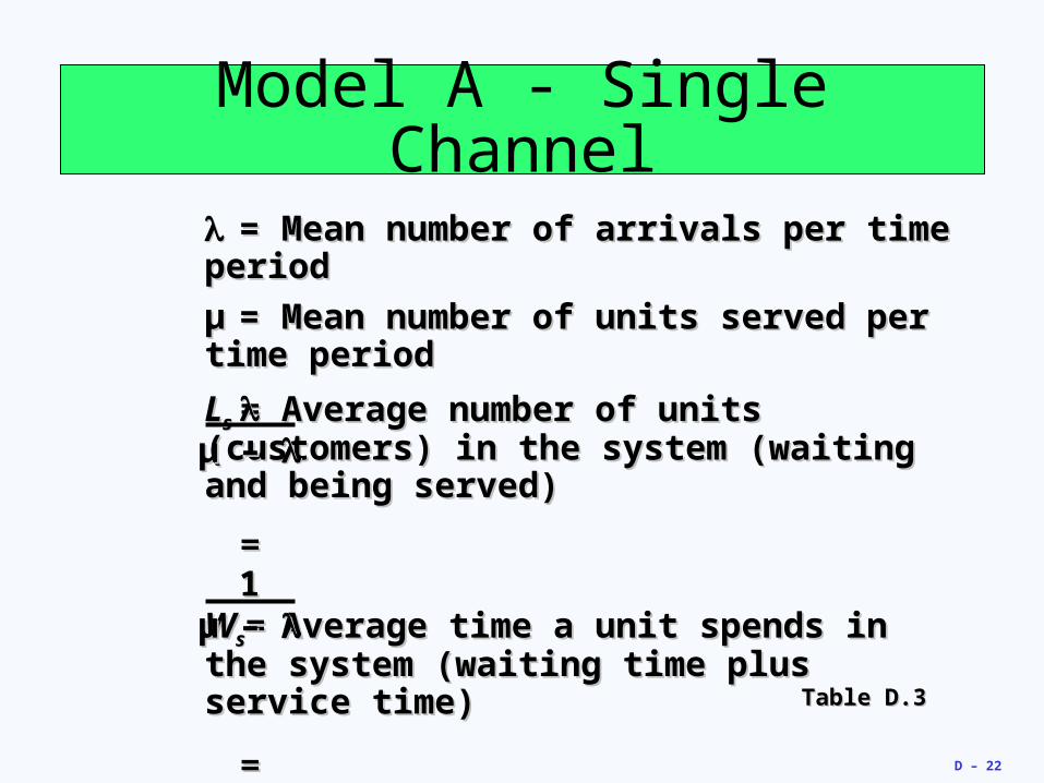
Model A - Single Channel
== Mean number of arrivals per time periodMean number of arrivals per time period
µµ == Mean number of units served per time Mean number of units served per time periodperiod
LLss == Average number of units (customers) in Average number of units (customers) in the system (waiting and being served)the system (waiting and being served)
==
WWss== Average time a unit spends in the Average time a unit spends in the system (waiting time plus service time)system (waiting time plus service time)
==
µ – µ –
11µ – µ –
Table D.3Table D.3
D – 23
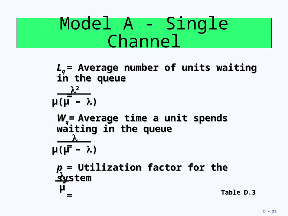
Model A - Single Channel
LLqq== Average number of units waiting in the Average number of units waiting in the queuequeue
==
WWqq== Average time a unit spends waiting in Average time a unit spends waiting in the queuethe queue
==
pp == Utilization factor for the systemUtilization factor for the system
==
22
µ(µ – µ(µ – ))
µ(µ – µ(µ – ))
µµ
Table D.3Table D.3
D – 24
Model A - Single Channel
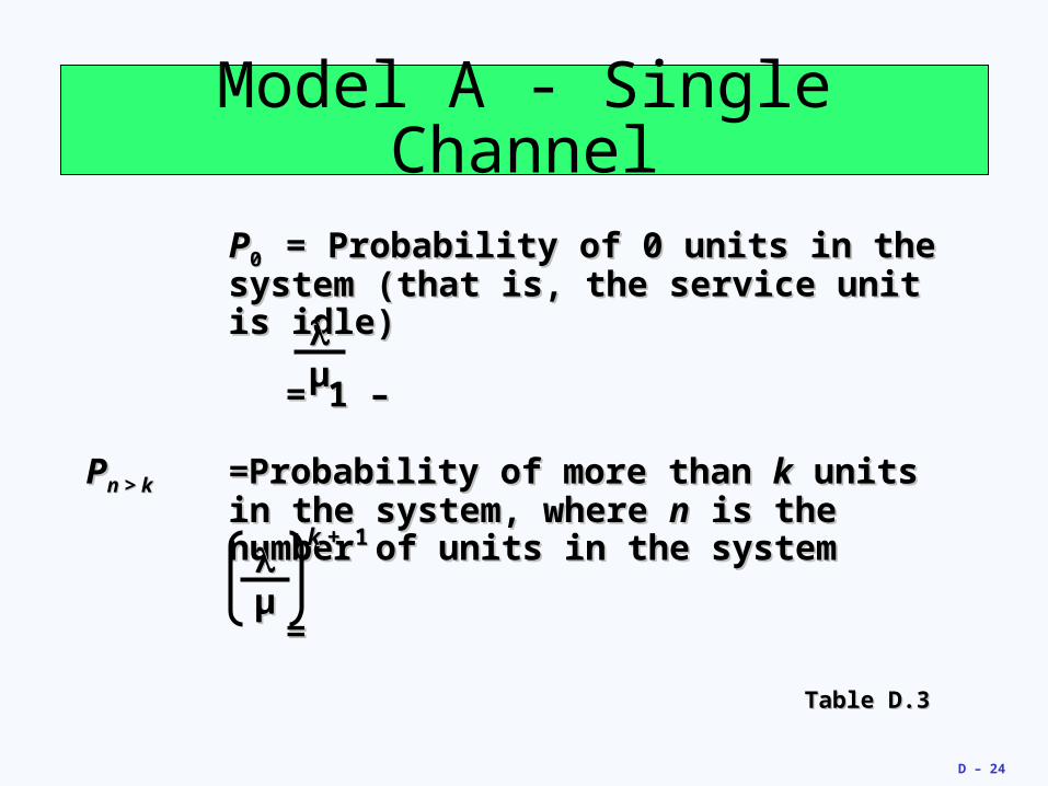
PP00 == Probability of 0 units in the system Probability of 0 units in the system (that is, the service unit is idle)(that is, the service unit is idle)
== 1 –1 –
PPn > kn > k ==Probability of more than Probability of more than kk units in the units in the system, where system, where nn is the number of units in is the number of units in the systemthe system
==
µµ
µµ
k k + 1+ 1
Table D.3Table D.3
D – 25
Single Channel Example
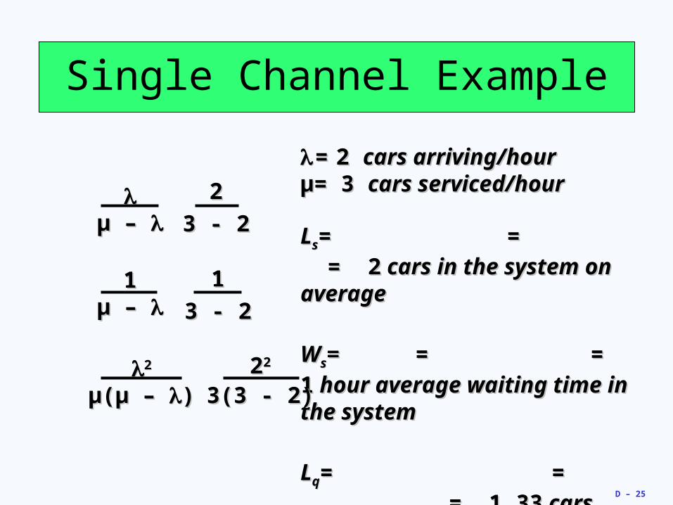
== 2 2 cars arriving/hourcars arriving/hourµµ= 3 = 3 cars serviced/hourcars serviced/hour
LLss= = = 2= = = 2 cars in cars in
the system on averagethe system on average
WWss = = = = 1= = 1 hour hour
average waiting time in the average waiting time in the systemsystem
LLqq== = = 1.33 = = 1.33
cars waiting in linecars waiting in line
22
µ(µ – µ(µ – ))
µ – µ –
11µ – µ –
22
3 - 23 - 2
11
3 - 23 - 2
2222
3(3 - 2)3(3 - 2)
D – 26
Single Channel Example
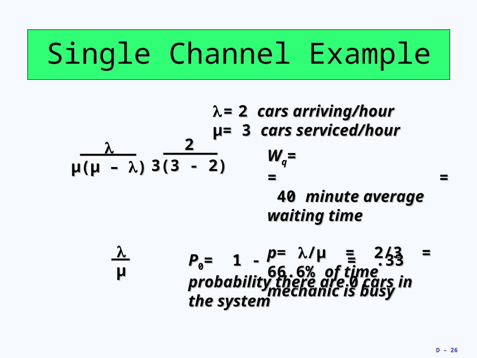
WWqq= = = =
= 40 = 40 minute average minute average waiting timewaiting time
pp= = /µ = 2/3 = 66.6% /µ = 2/3 = 66.6% of time mechanic is of time mechanic is busybusy
µ(µ – µ(µ – ))
223(3 - 2)3(3 - 2)
µµ
PP00= 1 - = .33= 1 - = .33 probability probability
there are there are 00 cars in the system cars in the system
== 2 2 cars arriving/hourcars arriving/hourµµ= 3 = 3 cars serviced/hourcars serviced/hour
D – 27
Single Channel Example
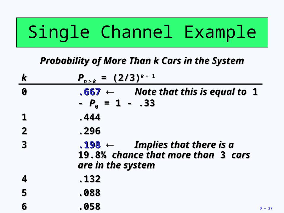
Probability of More Than k Cars in the SystemProbability of More Than k Cars in the System
kk PPn > kn > k = (2/3)= (2/3)k k + 1+ 1
00 .667.667 Note that this is equal toNote that this is equal to 1 - 1 - PP00 = 1 - .33 = 1 - .33
11 .444.444
22 .296.296
33 .198.198 Implies that there is aImplies that there is a 19.8% 19.8% chance that more thanchance that more than 3 3 cars are in the cars are in the systemsystem
44 .132.132
55 .088.088
66 .058.058
77 .039.039
D – 28
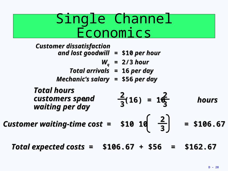
Single Channel EconomicsCustomer dissatisfactionCustomer dissatisfaction
and lost goodwill and lost goodwill = $10= $10 per hour per hour
WWqq = 2/3= 2/3 hour hour
Total arrivalsTotal arrivals = 16= 16 per day per dayMechanic’s salaryMechanic’s salary = $56= $56 per day per day
Total hours Total hours customers spend customers spend waiting per daywaiting per day
= (16) = 10 = (16) = 10 hourshours2233
2233
Customer waiting-time cost Customer waiting-time cost = $10 10 = $106.67= $10 10 = $106.672233
Total expected costs Total expected costs = $106.67 + $56 = $162.67= $106.67 + $56 = $162.67
D – 29
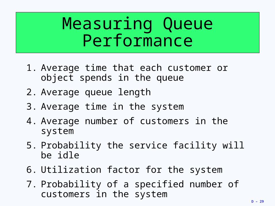
Measuring Queue Performance
1. Average time that each customer or object spends in the queue
2. Average queue length
3. Average time in the system
4. Average number of customers in the system
5. Probability the service facility will be idle
6. Utilization factor for the system
7. Probability of a specified number of customers in the system

D – 30
Queuing Models
Table D.2Table D.2
ModelModel NameName ExampleExample
BB Multichannel Multichannel Airline ticketAirline ticket (M/M/S) (M/M/S) counter counter
NumberNumber NumberNumber ArrivalArrival ServiceServiceofof ofof RateRate TimeTime PopulationPopulation QueueQueue
ChannelsChannels PhasesPhases PatternPattern PatternPattern SizeSize DisciplineDiscipline
Multi-Multi- SingleSingle PoissonPoisson ExponentialExponential UnlimitedUnlimited FIFOFIFO channelchannel
D – 31
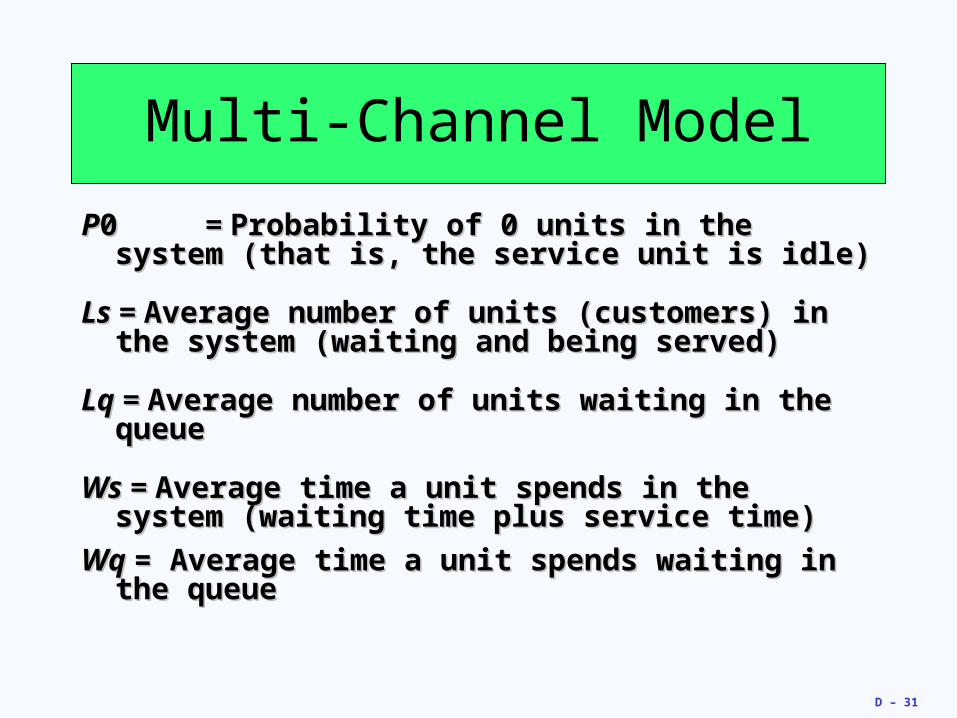
PP00 = = Probability of 0 units in the system (that Probability of 0 units in the system (that is, the service unit is idle)is, the service unit is idle)
Ls = Ls = Average number of units (customers) in the Average number of units (customers) in the system (waiting and being served)system (waiting and being served)
Lq = Lq = Average number of units waiting in the queueAverage number of units waiting in the queue
Ws = Ws = Average time a unit spends in the system Average time a unit spends in the system (waiting time plus service time)(waiting time plus service time)
Wq Wq = Average time a unit spends waiting in the = Average time a unit spends waiting in the queuequeue
Multi-Channel Model
D – 32
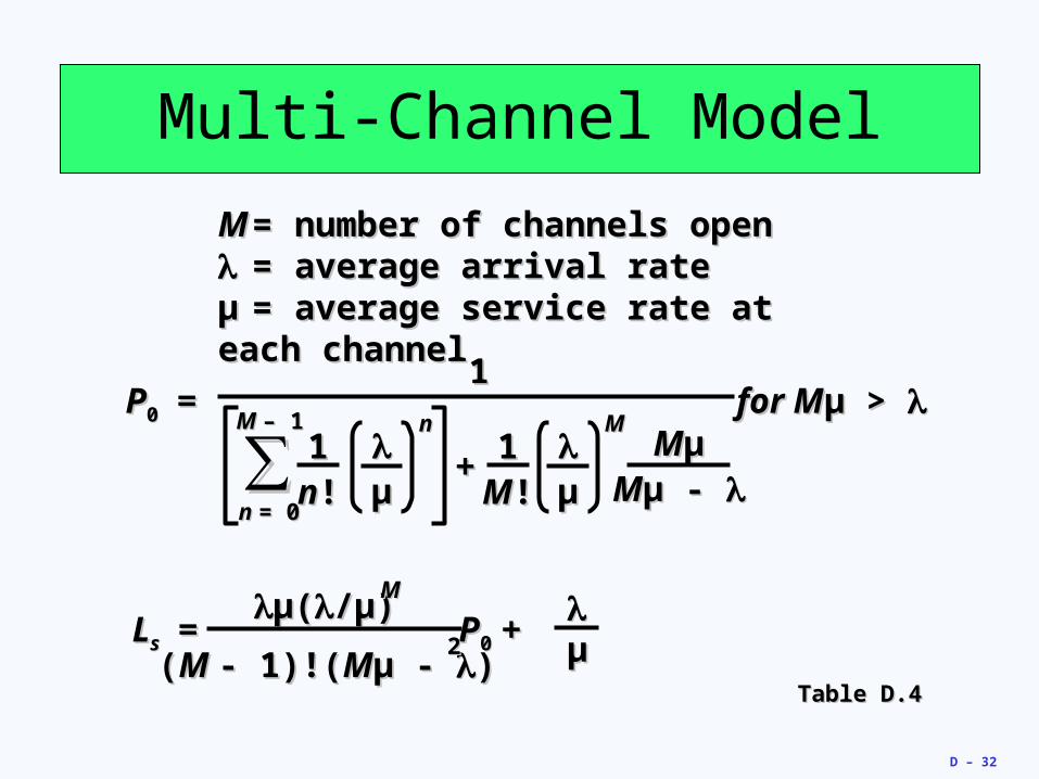
Multi-Channel Model
MM == number of channels opennumber of channels open == average arrival rateaverage arrival rateµµ == average service rate at each average service rate at each channelchannel
PP00 = for M = for Mµ > µ > 11
11MM!!
11nn!!
MMµµMMµ - µ -
M M – 1– 1
n n = 0= 0
µµ
nnµµ
MM
++∑∑
LLss = P = P00 + +µ(µ(/µ)/µ)MM
((M M - 1)!(- 1)!(MMµ - µ - ))22
µµ
Table D.4Table D.4
D – 33
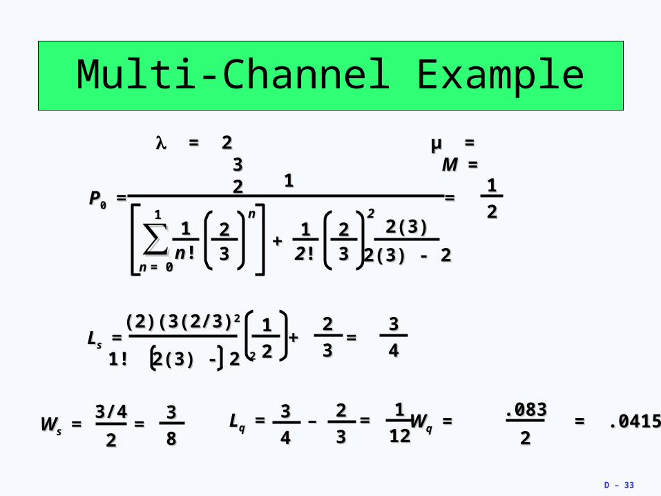
Multi-Channel Example
= 2 µ = 3 = 2 µ = 3 M M = 2= 2
PP00 = = = = 11
1122!!
11nn!!
2(3)2(3)
2(3) - 22(3) - 2
11
n n = 0= 0
2233
nn
2233
22
++∑∑
11
22
LLss = + = = + =(2)(3(2/3)(2)(3(2/3)22 22
331! 2(3) - 21! 2(3) - 2 22
11
22
33
44
WWqq = = .0415= = .0415.083.083
22WWss = = = =
3/43/4
22
33
88LLqq = – = = – =22
3333
44
11
1212
D – 34
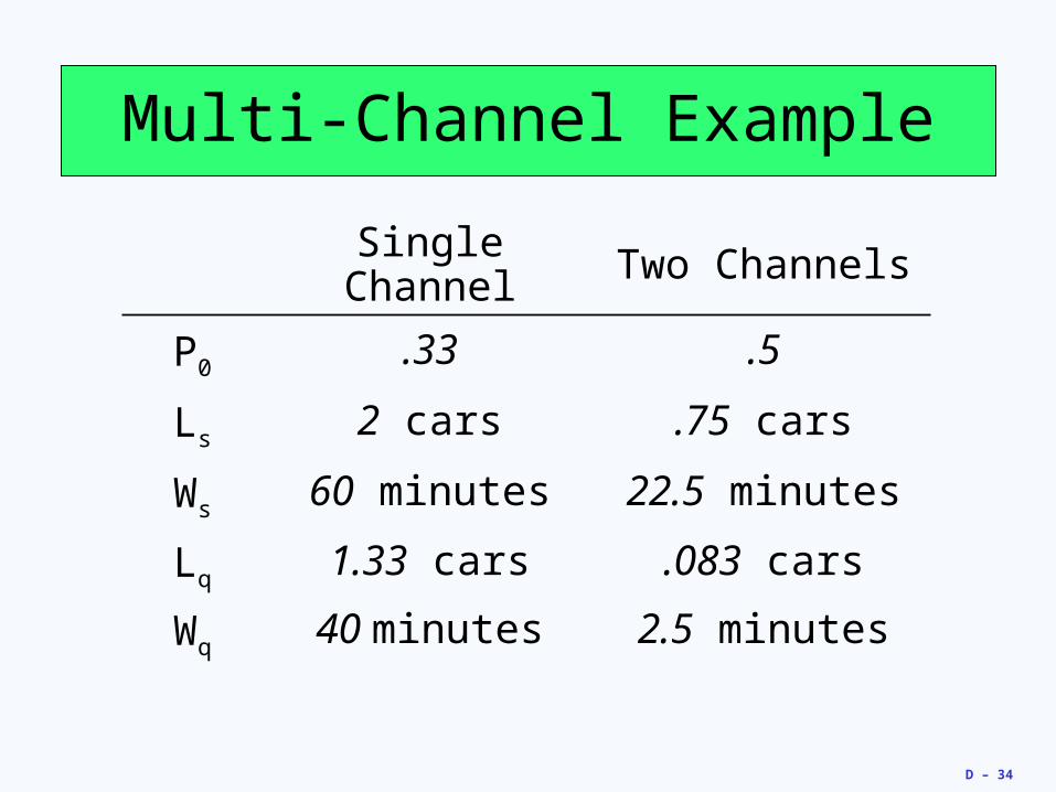
Multi-Channel Example
Single Channel Two Channels
P0 .33 .5
Ls 2 cars .75 cars
Ws 60 minutes 22.5 minutes
Lq 1.33 cars .083 cars
Wq 40 minutes 2.5 minutes
D – 35
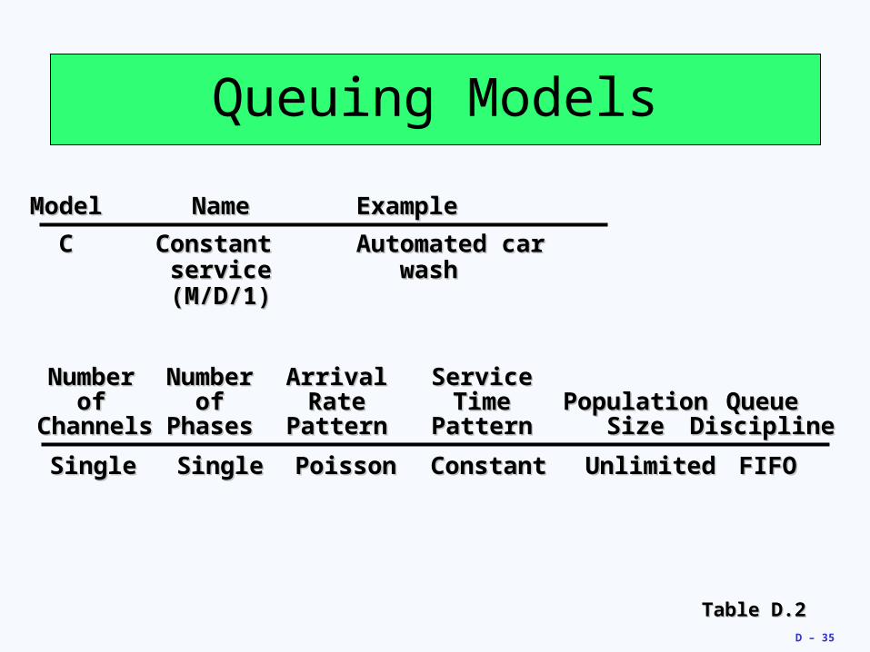
Queuing Models
Table D.2Table D.2
ModelModel NameName ExampleExample
CC Constant Constant Automated car Automated car service service wash wash(M/D/1)(M/D/1)
NumberNumber NumberNumber ArrivalArrival ServiceServiceofof ofof RateRate TimeTime PopulationPopulation QueueQueue
ChannelsChannels PhasesPhases PatternPattern PatternPattern SizeSize DisciplineDiscipline
SingleSingle SingleSingle PoissonPoisson ConstantConstant UnlimitedUnlimited FIFOFIFO
D – 36
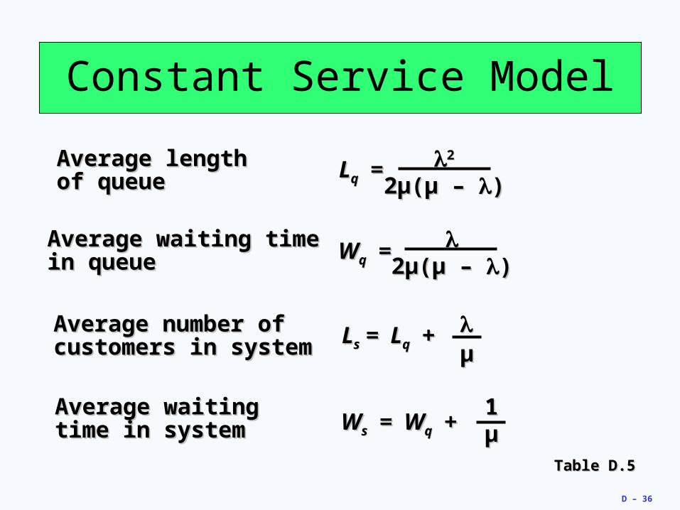
Constant Service Model
Table D.5Table D.5
LLqq = = 22
2µ(µ – 2µ(µ – ))Average lengthAverage lengthof queueof queue
WWqq = = 2µ(µ – 2µ(µ – ))
Average waiting timeAverage waiting timein queuein queue
µµ
LLss = L = Lqq + + Average number ofAverage number ofcustomers in systemcustomers in system
WWss = W = Wqq + + 11µµ
Average waitingAverage waitingtime in systemtime in system
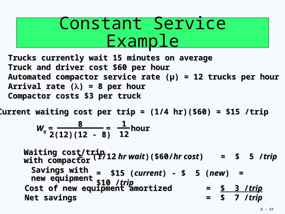
D – 37
Net savingsNet savings = $ 7 /= $ 7 /triptrip
Constant Service ExampleTrucks currently wait 15 minutes on averageTrucks currently wait 15 minutes on averageTruck and driver cost $60 per hourTruck and driver cost $60 per hourAutomated compactor service rate (µ) = 12 trucks per hourAutomated compactor service rate (µ) = 12 trucks per hourArrival rate (Arrival rate () = 8 per hour) = 8 per hourCompactor costs $3 per truckCompactor costs $3 per truck
Current waiting cost per trip = (1/4 hr)($60) = $15 /tripCurrent waiting cost per trip = (1/4 hr)($60) = $15 /trip
WWqq = = = = hourhour882(12)(12 - 8)2(12)(12 - 8)
111212
Waiting cost/tripWaiting cost/tripwith compactorwith compactor = (1/12= (1/12 hr wait hr wait)($60/)($60/hr costhr cost)) = $ 5 /= $ 5 /triptrip
Savings withSavings withnew equipmentnew equipment
= $15 (= $15 (currentcurrent) - $ 5 () - $ 5 (newnew)) = $10 = $10 //triptrip
Cost of new equipment amortizedCost of new equipment amortized = = $ 3 /$ 3 /triptrip
Recommended


![Heizer 9 ch8 f.ppt [Read-Only] - · PDF file© 2008 Prentice Hall, Inc. 8 – 1 Operations Management Chapter 8 – Location Strategies PowerPoint presentation to accompany Heizer/Render](https://img.pdfslide.net/doc/110x75/5a9dd7dd7f8b9a85318d5053/heizer-9-ch8-fppt-read-only-2008-prentice-hall-inc-8-1-operations.jpg)