Decentralized Robust Control of Robot Manipulators with Harmonic
Drive Transmission and Application to Modular and Reconfigurable
Serial Arms
Abstract
In this paper, we propose a decentralized robust control algorithm for modular and
reconfigurable robots (MRRs) based on Lyapunov’s stability analysis and backstepping
techniques. In using decentralized control schemes with robot manipulators, each joint is
considered as an independent subsystem, and the dynamical effects from the other links
and joints are treated as disturbance. However, there exist many uncertainties due to
unmodeled dynamics, varying payloads, harmonic drive (HD) compliance, HD complex
gear meshing mechanisms, etc. Also, while the reconfigurability of MRRs is
advantageous, modifying the configuration will result in changes to the robot dynamics
parameters, thereby making it challenging to tune the control system. All the above
mentioned disturbances in addition to reconfigurability present a challenge in controlling
MRRs. The proposed controller is well-suited for MRR applications because of its simple
structure that does not require the exact knowledge of the dynamic parameters of the
configurations. Desired tracking performance can be achieved via tuning a limited set of
parameters of the robust controller. If the numbers of degrees of freedom are held
constant, these parameters are shown to be relatively independent of the configuration,
and can be held constant between changes in configuration. This strategy is novel
compared to existing MRR control methods. In order to validate the controller
performance, experimental setup and results are also presented.
Index Terms
Modular and Reconfigurable Robot, robust, decentralized, Lyapunov,
backstepping.
Z. Li and W. W. Melek: University of Waterloo, 200 University Avenue West, Waterloo,
Ontario, Canada N2L 3G1
Email: [email protected] ; [email protected]
C. Clark: California Polytechnic State University, San Luis Obispo, CA 93407
Email: [email protected]

I. INTRODUCTION
Robot manipulators have served the manufacturing industry for many years. But due to
the fast growth of the economy, the conventional fixed-anatomy robots will not satisfy
the requirements of a transition from mass to customer-oriented production. To respond
to rapid changes of product design, manufacturers need a more flexible fabrication
system. A commonly used method is to use programmable robots that are expensive, and
limited by hardware constraints. In recent years, modular and reconfigurable robots
(MRRs) [1][2] were proposed to fulfill the requirements for the flexible production
system. The majority of the associated research is geared towards self-reconfigurable
robots [3][4]. At present, the application of reconfigurable robots in manufacturing is
quite limited. However recent technology and research advances are very promising. As
an extension of the concept of a modular robot system, the MRR system is referred to the
entire manipulator system that includes not only the modular mechanical hardware, but
also modular electrical hardware, control algorithms and software [2]. In [5], an MRR
system is defined as a collection of individual link and joint components that can be
easily assembled into a variety of configurations and different geometries. In [6], the
author states that in the near future the MRR system will mostly replace current fixed
configuration industrial robots.
Except for reconfigurability requirements, lighter manipulators that can handle heavier
payloads have brought more attention to both robot designers and industrial
manufacturers. To achieve this, harmonic drives (HD) have been widely used in robotic
system design due to its compact size, zero back-lash, light weight, high torque
transmission [1][2][7]. Unfortunately they exhibit drawbacks including the flexspline
elasticity, and complex meshing mechanisms between the flexspline and circular spline.

MRRs with HDs have more uncertainties in the mechanical system. Therefore, to control
such a system is more challenging. The selection of the control law not only depends on
the robot mechanical design, i.e. rotary joint robot and Cartesian manipulator, but also
relies on the model used. Based on the assumption made on the manipulator's joints,
links, and the control signal, six manipulator models are commonly encountered in the
literature: 1) torque level rigid link rigid joint (TLRLRJ) [8][9][10]; 2) electrically driven
rigid link rigid joint (EDRLRJ) [11]; 3) torque level rigid link flexible joint (TLRLFJ)
[12][13][14]; 4) electrically driven rigid link flexible joint (EDRLFJ) [15]; and 5) flexible
manipulator (FM) [16]. A considerable number of control techniques and methodologies
have been created and applied to the control of manipulators. In this paper, the controller
development for MRR systems is based on TLRLFJ.
Joint flexibility is a major source of oscillatory behaviour of the manipulator, and
considerably affects a robot's performance. A widely acceptable TLRLFJ model was
introduced in [17], where the robot was modeled as two second order differential
equations under the assumption of 1) the joints are purely rotary; and 2) the rotor/gear
inertia is symmetric about the rotation axis. This dynamic model was shown to be
globally linearizable and a nonlinear control was provided based on a singular
perturbation formulation of the equations of motion and the concept of integral manifold,
but the author did not prove the stability of the system. Based on the same theories, a
composite control algorithm with detailed stability analysis was proposed in [14], which
consists of a fast control and a slow control. In [18], a fuzzy supervisor was added to
decrease the fast controller bandwidth at critical occasions, i.e. near saturation point
which could cause instable.
Robust control is a commonly used strategy to control complex systems, especially for
robot manipulators. [19] presents a summary of robust control method before 1997 in the
categories of linear, passivity-based, Lyapunov-based, sliding mode, nonlinear and robust
adaptive control schemes. [20] provides detailed design procedure of centralized
Lyapunov-based robust control for an n-dof manipulator under joint flexibility. [21]
standardizes some robust controller, such as saturation type controller, passivity
controller, etc. For decoupled joint controller, each joint is considered as a single input
single output (SISO) subsystem. A general form of decentralized sliding mode robust
control law is proposed in [23] for any mechanical system described by Euler-Lagrange
equation and involving high-order interconnections. In [24], another simple decentralized
nonlinear control algorithm was developed. This controller had three integral terms in the
tracking error, and a systematic method for controller parameters selection is also
provided. But those controllers [23][24] were designed for TLRLRJ. In [22] a linear
PD/PID compensator has been designed by considering actuator saturation and
transmission flexibility. Other controllers, such as PD/PID with gravitational
compensation, intelligent fuzzy controller, etc., can be found in [25][26][27][28][29].
To the best of our knowledge, there exists very limited research dedicated to control of
MRRs. This is most likely because a new configuration of the robot results in a new set
of robot dynamic parameters. In [30], an MRR control approach is proposed that focuses
on the “high-level” analysis of the feasibility of a decentralized strategy that handles
serial arms as a group of 1 DOF defective joints. Unlike the approach in [30], this paper
presents a decentralized robust controller for MRRs with HD that uses Lyapunov-based
method and backstepping techniques. Furthermore, unlike the control software presented
in [31] which requires configuration dependent parameters, our proposed controller is
configuration independent. Therefore, the proposed controller will enable fast
reconfigurability of the manipulator as well the control strategy to achieve precise
position tracking in the task space of the manipulator.
The organization of the paper is follows: Section II introduces the dynamic model.
Section III describes the controller design. Section IV provides the experiments setup and
results. The conclusions are documented in Section V.
II. MRR SINGLE JOINT MODEL
A commonly used model for an n-dof of torque level rigid link flexible joint (TLRLFJ)
model is introduced in [17] in the form of:
0)(),()( 211111 qqkqqCqqD (1)

uqqkqJ )( 212 (2)
Where, )( 1qD is a nn symmetric, positive definite inertial matrix. The vector
),(11 qqC contains coriolis, centripetal, friction and gravitational forces and torques. k
and J are the nn diagonal stiffness coefficients and motor inertial matrix, respectively.
For the development of the decentralized control scheme, most papers [12][25] are based
on the above two equations and consider the inertial coupling term, the Coriolis,
centrifugal, friction and gravity terms in (1) as a disturbance torque. In this paper, a
decentralized controller is designed based on single joint dynamics including friction,
gravity and compliance.
A single joint with harmonic drive (HD) can be modeled as a mass-spring system with
three subsystems: 1) motor and wave generator (input) subsystem; 2) flexspline
(transmission) subsystem; 3) link and load (output) subsystem.
By applying Euler-Lagrange theorem, three equations can be derived for each subsystem
(see Appendix):
fmsmdmw NqsignFqFqJ )( 222 (3)
fss qNqKqNqK 3
122121 )()( (4)
0))(()( 1111 fdlsldl qsignFqFqsignmglqJ (5)
In this model, the HD flexspline compliance is modeled as a nonlinear cubic function
[32][33] as shown in (4). Substituting (4) into (3) and (5) yields two equations
representing the single joint dynamics:
3
122121222)()( qNqNKqNqNKqsignFqFqJ ssmsmdmw (6)
dsslsldl qNqKqNqKqsignFqFqmglqJ 3
1221211111)()()()sin(0 (7)
Notations used in (6) and (7) are:
mwJ - motor rotor and HD wave-generator inertial
msmd FF , - input dynamic and static friction coefficients

21, ss KK - flexspline stiffness coefficients
222 ,, qqq - motor position, velocity and acceleration
N - HD gear reduction ratio
- motor input torque
lJ - output side inertia (link, load)
m - link mass
l - link length
lsld FF , - output side dynamic and static friction coefficients
111 ,, qqq - link position, velocity and acceleration
d - disturbance torque
III. CONTROLLER DESIGN
We can use two cascaded subsystems representing motor dynamics (6) and robot
dynamics (7), respectively, as shown in Fig. 1. The first subsystem of motor dynamics
has the input , the motor control torque, and outputs, 22 ,qq and 2q , the motor states.
The motor position 2q is considered as the input to the second subsystem of robot
dynamics which outputs 11,qq and 1q , the link states. The robot control signal 2q is not
the control signal that is sent to the system. In this situation, the backstepping [34]
method is to be used, and the robot input signal 2q is called the fictitious control signal
[20]. The motor or system input signal is called the system control signal. In order to
design the system control signal , the fictitious control signal needs to be selected first,
then stepped back to the system control signal. Both fictitious control and system control
signal are designed based on the Lyapunov direct method. The proposed control law
consists two terms: 1) a linear PD control, and 2) a nonlinear term to compensate for
disturbances to the system.
To develop the controller, we introduce the following preliminary definitions [20] made
on parameters in equations (6) and (7).

~
0: JJInertia (8)
qFFqFqFFriction ds 21)(: (9)
ii KKyFlexibilit~
0: (10)
~
0:eDisturbanc (11)
Where ~
J and iK~
present the largest motor/link inertia and the largest stiffness
coefficients of the MRR, respectively and ~
is the maximum disturbance.
A. Fictitious Control Law Selection
Suppose that the manipulator joint is required to track a desired joint angle dq1 which has
at least third order differentiability so that the desired velocity d
q1 and desired
acceleration d
q1 exist and can be derived from the derivative of dq1 .The link error
dynamics are calculated by adding d
l qJ1 on both sides of (7), and after some
manipulation, the link error dynamics can be formed as:
])()sin()([)( 21
3
12211111
1
111 NqKqNqKqKqmglqsignFqFJqe sdsslsld
d
(12)
Let
dsslsld qNqKqKqmglqsignFqFqqqf 3
12211111211)()sin()(),,(
(13)
So equation (12) can be simplified as:
]),,([)( 21211
1
111 NqKqqqfJqe s
d (14)
The function ),,( 211qqqf includes all the uncertainties of the link dynamics, i.e. friction,
stiffness and load disturbance. Based on assumptions made in equation (9)-(11), the
bounded uncertainty can be calculated:

f
qNqKqKqKK
qNqKqFqKmglF
qNqKqFqKqmglqsignFqqqf
sldsdls
sldsdls
3
121311211110
3
122111
3
12211111211
)(
)(
)()sin()(),,(
(15)
3
121311211110 )( qNqKqKqKKf (16)
The fictitious control signal 2q in (14) can be chosen in the following form [20]:
r
s
d
s
l uNK
eKeKqNK
Jq
1
12111
1
2
1)( (17)
Where 0,0 11 KKs and 02K are linear PD control gains, and ru is an additional
term designed to compensate the nonlinear uncertainties. Substitute (17) into (14), and
the closed loop link error dynamics are:
)),,(()( 211
1
112111 ruqqqfJeKeKe (18)
To find the nonlinear term ru , the following Lyapunov function candidate is considered
[20]:
2
12
11
'1
2
1
2
1eeKV (19)
Clearly, it is positive definite, and 1K is the same PD control gain as shown in (17). Take
the derivative on both sides and substitute (18) into it, we can have:
)()(
)()(
))()((
11
1
2
12
11
1
2
12
1
112111111
11111
'1
r
r
r
ufeJeK
ufeJeK
ufJeKeKeeeK
eeeeKV
(20)
If we select fur , then 0'
1V is guaranteed. Therefore, the fictitious control law is:

fNK
eKeKqNK
Jq
s
d
s
l
1
12111
1
2
1)( (21)
Equation (21) represents the fictitious control law, which is a saturation type control [21]
because the nonlinear term f is bounded.
B. Backstepping
The fictitious control law has been selected, but it needs to be backstepped to the side of
the motor dynamics subsystem. To do so, we can add and subtract NKJ sl 1
1)( to the
right side of (14), where denotes the fictitious control variable:
)()()()( 21
1
11
1
111 qNKJNKfJqe ss
d (22)
Equations (22) and (6) form the new dynamics of the single joint. If 02q , then
equation (22) is stable since is a robust controller, as shown above. Therefore, our goal
is to design robust control law in equation (6) such that 2q either converges to zero
or at least is bounded by a small constant. The following Lyapunov candidate for the
overall system is used [20]:
2
2
22
2
23
21
2
11
321
)(2
1])(
2
1
2
1[])(
2
1
2
1[ qeeKeeK
VVVV
(23)
Where, 03K is another PD controller gain which will be defined later. Replacing 1e by
new error dynamics (22) and substituting the fictitious control yields:

)()(
)()()()()(
)()(
)]}1
)(([)({
))()(][)((
211
1
2
12
211
11
112111111
211
1
1
12111
1
1
1
111111
21
1
1
1
11111
111111
qeNKJeK
qeNKJffeJeKeKeeeK
qeNKJ
fNK
eKeKqNK
JNKfJqeeeK
qNKJNKfJqeeeK
eeeeKV
sl
sll
sl
s
d
s
ls
d
slsl
d
(24)
In order to calculate the derivative of 2V , the motor error dynamics need to be formed.
Add d
mw qJ 2 to both sides of (6) and perform some simple manipulation, we have:
3
12212122222 )()()()( qNqNKqNqNKqsignFqFqJqqJ ssmsmd
d
mw
d
mw
]),,([ 122
1
22 qqqgJqe mw
d
(25)
Similar to ),,( 211qqqf in (16), ),,( 122
qqqg contains all the uncertainties of the motor
dynamic subsystem, i.e. motor rotor friction, flexspline compliance, and the upper
bounded function is defined as:
3
12212122122)()()(),,( qNqNKqNqNKqsignFqFqqqg ssmsmd (26)
3
1223122222120122)()(),,( qNqKqNqKqKKqqqg
(27)
Similar to the fictitious control law in (17), the control signal can be chosen as [20]:
124232 )( ueKeKqJd
mw (28)
Where 03K and 04K are the linear PD gains, and 1u is a nonlinear term to
guarantee 0V while not 02V itself. Take the derivative of 2V and substitute (25),
(26) and (28), we have:
)(
)()(
]})([{
))((
121
2
24
121
24232223
124232
1
22223
1
22223
222232
ueJeK
ueJeKeKeeeK
ueKeKqJgJqeeeK
gJqeeeK
eeeeKV
mw
mw
d
mwmw
d
mw
d
(29)
Finding 3V is not a straightforward task because 3V in (23) is a function of the fictitious
control law . As shown in (21), is a function of desired link acceleration, link
position error, link velocity error and bounded function . Therefore, the derivative of 3V
introduces link acceleration error which can be very difficult to measure. The following
calculation is targeted at eliminating the link acceleration error term.
We can consider the simple form of 3V
))((223 qqV (30)
V can be formed by combining (29), (30) and (24), that is:
121
21
11
1
22
2
24
2
12
121
21
11
1
22
2
24
2
12
22121
2
24211
1
2
12
))((
))()((
))(()()()(
ueJeJeNKJqqeKeK
ueJeJeNKJqqeKeK
qqueJeKqeNKJeKV
mwmwsl
mwmwsl
mwsl
(31)
To find 1u , needs to be calculated first from (21)
fNK
eKeKqNK
J
s
d
s
l
1
1211
)3(
1
1)(
1 (32)
From (15) we can calculate f
)()(312
2
1213112111 qqNqNqKqKqKf (33)
Substitute (33) into (32)

1122
1
1111
1
12
2
1213
1
111
1
112
1
)3(
1
12
2
1213
1
112
1
112
1
111
1
111
1
1211
)3(
1
12
2
1213
1
112
1
111
1
1211
)3(
1
12
2
1213112111
1
1211
)3(
1
)(1
)(1
)()(311
)()(3
1111)(
)()(3
11)(
)]()(3[1
)(
1
1
1
1
eKKJNK
eKKJNK
qqNqNqKNK
qKNK
qKNK
qNK
J
qqNqNqKNK
eKNK
qKNK
eKNK
qKNK
eKeKqNK
J
qqNqNqKNK
qKNK
qKNK
eKeKqNK
J
qqNqNqKqKqKNK
eKeKqNK
J
l
s
l
s
s
d
s
d
s
d
s
l
s
s
d
ss
d
s
d
s
l
s
ss
d
s
l
s
d
s
l
(34)
Therefore,
1122
1
1111
1
12
2
1213
1
10
11
1
10
12
1
)3(
01
1122
1
1111
1
12
2
1213
1
111112
1
)3(
1
11
)(3
sup1
sup1
sup
11
)(3
][1
1
1
eKKJNK
eKKJNK
qqNqNqKNK
qKNK
qKNK
qNK
J
eKKJNK
eKKJNK
qqNqNqKNK
qKqKNK
qNK
J
l
s
l
s
s
d
ts
d
ts
d
ts
l
l
s
l
s
s
dd
s
d
s
l
(35)
The following observations can be made:
If 0122 KKJ l is satisfied by choosinglJ
KK 12
2 , 1e can be eliminated.
Because the flexspline elastic displacement is very small (e.g. in 410 rad range),
and can be determined by experiments, we can therefore assume

12
2
1213
1
)(3
qqNqNqKNK s
is small and bounded. Let
12
2
1213
1
10
1110
12
)3(
01
30 )(3
]supsupsup[1
1qqNqNqK
NKqKqKqJ
NKK
s
d
t
d
t
d
tl
s
Let
111
1
31
1KKJ
NKK l
s
By applying the above observations to (35), we have:
1
3130 eKK (36)
Substitute (36) into (31), and consider 222 eqq d , we have:
}))(()(sup{
})({
211
1
313020
2
121
21
2
24
2
12
11
113130222
121
21
2
24
2
12
eeNKJKKqq
ueJeJeKeK
eNKJeKKeqq
ueJeJeKeKV
sl
d
t
mwmw
sl
d
mwmw
(37)
Ideally, 21 eNe , therefore we can find a '
31K to satisfy
}))({( 211
1
312'
31 eeNKJKJeK slmw (38)
Let
)(sup 3020
'
30KqJK d
tmw (39)
Equation (37) can be simplified to:

121
21
22
'
31
1
2
'
30
1
2
24
2
12
121
21
2
'
31
'
302
1
2
24
2
12 )(
ueJeJeqKJqKJeKeK
ueJeJeKKqJeKeKV
mwmwmwmw
mwmwmw
(40)
We can choose nonlinear term 1u in the form of
)( 2
'
312
'
30
322
233
1 qKqK
Ke
eKu (41)
Substitute (41) into (40), the final V is
))((
)1(
2
'
31
322
2
233
21
322
2
233
2
'
30
1
2
24
2
12
qK
Ke
eK
eJ
Ke
eK
qKJeKeKV
mw
mw
In order to satisfy the above inequity, let 033K and 232 eK . And
))((
)(
2
'
31
322
2
233232
2
2
1
322
2
233322
2
'
30
1
2
24
2
12
qK
Ke
eKeKe
J
Ke
eKKe
qKJeKeKV
mw
mw
(42)
Because 32K and 33K are control parameters, we can choose suitable values to ensure

232
2
2
2
233
322
2
233
eKeeK
KeeK
Therefore, we can achieve 0V . This implies uniformly ultimate bounded stability
given the fact that 33K increases as 2e decreases. Substitute (41) into (28), the final
control torque is:
)()( 2
'
312
'
30
322
23324232 qKqK
Ke
eKeKeKqJ d
mw (43)
For MRR, the configuration change presents a new set of robot dynamic parameters.
Hence, decentralized control is a suitable strategy to handle motion tracking of MRR. In
decentralized control, every joint is treated as a single input single output (SISO) system
plus a disturbance torque representing all uncertainties of the robot. In equation (43), 33K
and 32K are control parameters; '
30K , 31K and are determined based on the upper
bound on the link/motor dynamics. Therefore, (43) does not directly depends on the link
parameters and will require minimal (or no) change of control parameters when robot is
reconfigured. The proposed control law is a saturation type controller because of the
bounded nonlinear term 1u .
IV. EXPERIMENT
The performance of the proposed robust controller was evaluated using a three degree of
freedom (DOF) modular and reconfigurable robot (MRR) controlled by a MSK2812 DSP
kit. For every DOF, joint parameter identification was performed according to the
procedure described in [35]. Two different configurations with and without load were set
up. For each case, the MRR was controlled to follow sinusoidal trajectories in joint space
using the same set of control parameters. The experimental setup and results are
presented in this section.

I. MRR System
The MRR system block diagram is shown in Fig. 2. Block diagram of MRRFig. 2. All
three joints are connected with DSP via controller area network (CAN) communication
bus, and the DSP is connected with a PC through RS232. Each joint accepts the torque
command transmitted on the CAN based on its own ID, and sends the motor and link
position/velocity signals back to DSP for both closed loop control and data collection.
This data can be uploaded to a PC offline. Because of the limit of CAN bus, the control
frequency is less than standard 500Hz. The desired trajectory for each joint is in the form
of:
))(*2
sin(f
j
TATraj (44)
Where, deg90A is the trajectory amplitude, sT 7 is the trajectory period, Hzf 50
is the control frequency, and ,...1,0j is the control signal index. Fig. 3 and Fig.
4Error! Reference source not found. show the desired trajectories of both
configurations in the task space. These trajectories map to sinusoidal trajectories for each
joint in joint space. Fig. 5 and Fig. 6 show two different MRR configurations. For each
configuration, two tasks were tested under load and no load conditions. The load is in the
form of a wrist assembly that weighs 20lb as shown in Fig. 5 and Fig. 6.
II. Experiment Results
Parameters of the proposed controller were tuned to reduce the trajectory tracking error
based on the first configuration without load, while satisfying the constraints described in
Section III. We first tuned PD gains, 3K and 4K in equation (43), to achieve a desirable
tracking performance. Then the nonlinear term was added to compensate disturbances
and tuned to achieve the desired trajectory tracking performance. These same set of
parameters were then applied to all other experiments, i.e. with load and for the second
configuration. The parameters are listed in Table. I. 2,1, ikij and 4,3,2,1j , were
not shown in this table, because they were calculated from equation (16) and (17),
respectively. The mean squared error (MSE) shown in equation (45) was used to evaluate
the MRR trajectory tracking performance. Equation (46) was used to calculate the

improvement of the proposed robust controller compared to PID controller. The results
are summarized in Tables II and III for both configurations.
N
MqMSE
ijij aa
N
j
i
2
1 )( (45)
Where N is the number of sampled data, 3,2,1i refers thi joint, and ijaq and
ijaM are
the measured position errors and mean of those errors of each joint, respectively.
%100)(
)()(
MSEPID
MSERobustMSEPIDtimprovemen (46)
From Table II, it can be shown that for configuration 1 the proposed robust controller
outperformed the well-tuned linear controller for all three degrees of freedom. For the
given trajectory in Fig. 3 and Fig. 4Error! Reference source not found., the
improvement in performance at no load is 38.92%, 8.93% and 27.20% for joints 1, 2, and
3 respectively. For a payload of 20Lb in the form of an end point wrist assembly, the
improvement in performance using the robust controller is 16.35%, 14.92%, and 5.04%
for joints 1, 2, and 3 respectively. Under reconfiguration, all control parameters in Table I
were kept unchanged. The robust control still outperformed the industrial linear control
for the configuration 2 shown in Fig. 6. For the trajectory shown in Fig. 3 and Fig.
4Error! Reference source not found., the robust control showed an improvement in
tracking performance of 12.17% for joint 1, 16.24% for joint 2 and 45.53% for joint 3 at
no load. With a 20Lb end point load, the improvement in tracking performance is 6.91%
for joint 1, 11.79% for joint 2 and 26.26% for joint 3. The percentage improvements in
workspace tracking using the proposed controller compared to PID controller for a 20 Ib
end point load are summarized in Table 4.
During experiments it was observed that the first joint is the most rigid compared to
others, and the third joint generated more vibrations because of dynamic interactions with
other degrees of freedom joints. Fig. 7 - Fig. 18 show the torque signals of each joint of
both configurations under different tasks.
V. CONCLUSION

In this paper, a decentralized robust controller is presented for a modular and
reconfigurable robot (MRR) that uses a harmonic drive transmission system. The
uncertainty compensation and good position tracking performance is achieved by fusing a
linear PD controller with a saturated type robust control law. In order to precisely control
the MRR, the nonlinear property of HD flexspline compliance was introduced into the
joint dynamics (6) (7). The important features of the controller are the simplicity in
computation compared with a centralized controller, and greater disturbance tolerance
which can be observed from the successful position tracking during experimental
analysis.
APPENDIX
SINGLE JOINT DYNAMIC
The detailed derivations of the single joint dynamic equations of (3) (4) and (5) are
shown in this appendix. The single joint with HD can be modeled as a mass-spring
system as shown in Fig. 7, and it is considered as three subsystems: 1) input subsystem;
2) transmission subsystem; and 3) output subsystem. All the notations can be found in
Section II.
A. Input subsystem
The input subsystem consists of motor and HD wave-generator, based on Euler-Lagrange
equation, we have:
Kinetic energy: 2
22
1qJK mw
Potential energy: 0P
Lagrangian: 2
22
1qJPKL mw
Therefore the resulting torque can be calculated as:

2
22
qJq
L
q
L
dt
dmwm (47)
This resulting torque m is also related to motor input torque , friction torque and
flexspline stiffness torque exerted on the input side. The following equation is satisfied:
fmsmdm NqsignFqF ))(( 22 (48)
Therefore, the input subsystem dynamic equation is:
fmsmdmw NqsignFqFqJ )( 222 (49)
B. Transmission subsystem
The transmission subsystem refers to the flexible HD flexspline which is usually run at
low speed, and its mass can be ignored. Two types of flexspline models are widely used,
piece-wise linear [37] and nonlinear [36]. We have setup experiments to calibrate the
flexspline stiffness coefficients, and found that a nonlinear model better represents the
flexspline dynamics. The experiments and results are out of the scope of this paper. The
flexspline dynamics is in the following form:
3
122121 )()( qNqKqNqK ssf (50)
C. Output subsystem
The link and load together form the output subsystem. The link generates great effects on
the robot dynamics. In comparison with the unexpected load which is exerted at the end
of the link, the link mass is very small. Therefore, we assume the link mass m is centered
at the end of the link as shown in Fig. 7. Based on the Euler-Lagrange equation:
Kinetic energy: 2
12
1qJK l
Potential energy: )cos( 1qmglP
Lagrangian: )cos(2
11
2
1 qmglqJPKL l

The resulting torque is:
)sin( 11
11
qmagqJq
L
q
L
dt
dll (51)
The resulting torque l comes from the torsional torque applied by the flexspline, friction
torque and disturbance, which can be expressed as:
dlsldfl qsignFqF ))(( 11 (52)
So the output dynamics is
0))(()( 1111 fdlsldl qsignFqFqmglsignqJ (53)
Finally, we can rearrange (49), (50), (53) into two equation representing single joint
dynamics in (6) and (7).

Table 1
ROBUST CONTROLLER PARAMETERS
Linear parameters Nonlinear parameters
Joint 3K 4K 30K 31K 32K 33K
#1 0.25 0.025 0.1 0.2 1 0.12
#2 0.15 0.005 0.1 0.1 1 0.8
#3 0.35 0.025 0.1 0.2 0.01 0.3
Table 2
CONFIG 1: PID vs ROBUST
Joint No load (position MSE) Load 20lb (position MSE)
PID
(deg2)
Robust
(deg2)
Improve
(%)
PID
(deg2)
Robust
(deg2)
Improve
(%)
#1 1.4445 0.8823 38.92 1.1562 0.9672 16.35
#2 1.8327 1.3025 28.93 2.7272 2.3202 14.92
#3 1.0856 0.7903 27.20 1.9009 1.8052 5.04
Table 3
CONFIG 2: PID vs ROBUST
Joint No load (position MSE) Load 20lb (position MSE)
PID
(deg2)
Robust
(deg2)
Improve
(%)
PID
(deg2)
Robust
(deg2)
Improve
(%)
#1 0.9900 0.8695 12.17 1.6999 1.5825 6.91
#2 1.9590 1.6409 16.24 3.8442 3.3910 11.79
#3 2.3647 1.2880 45.53 4.6938 3.4610 26.26
Table 4
Percentage Improvement of tracking In Workspace coordinates
Config. Load Position
(X) %
Position
(Y) %
Position
(Z) %
Rotation
(X) %
Rotation
(Y) %
Rotation
(Z) %
20 Ib 25.97 15.57 12.28 -5.62 28.19 6.50
20 Ib 35.66 21.01 47.14 27.75 22.44 30.38

Fig. 1. System block diagram
Fig. 2. Block diagram of MRR

Fig. 3 Configuration 1 end effector trajectory in workspace

Fig. 4 Configuration 2 end effector trajectory in work space

Fig. 5. Configuration 1: with load
Fig. 6. Configuration 2: with load

Fig. 7. joint 1 torque (config 1 no load)

Fig. 8. joint 2 torque (config 1 no load)

Fig. 9. joint 3 torque (config 1 no load)

Fig. 10. joint 1 torque (config 1 with load)

Fig. 11. joint 2 torque (config 1 with load)
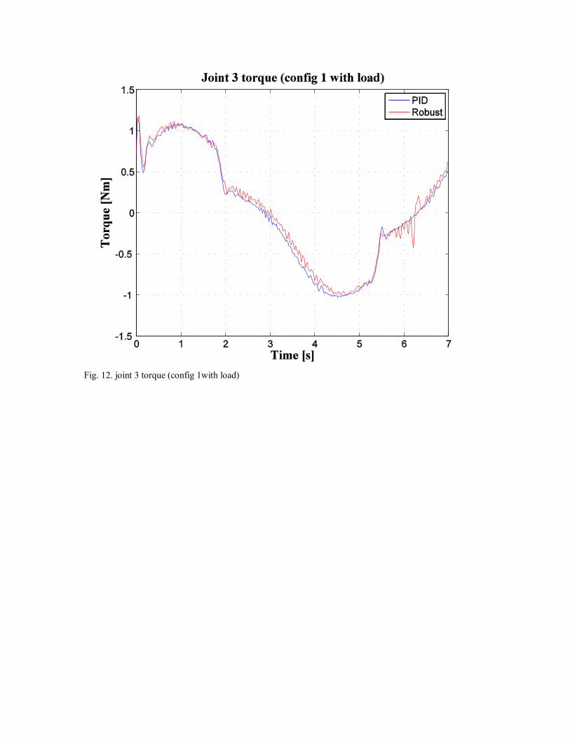
Fig. 12. joint 3 torque (config 1with load)

Fig. 13. joint 1 torque (config 2 no load)

Fig. 14. joint 2 torque (config 2 no load)

Fig. 15. joint 3 torque (config 2 no load)
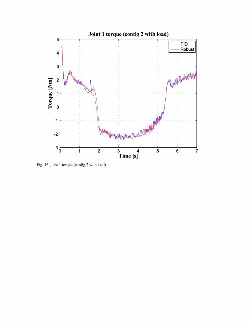
Fig. 16. joint 1 torque (config 2 with load)

Fig. 17. joint 2 torque (config 2 with load)

Fig. 18. joint 3 torque (config 2 with load)

Fig. 19. Joint model
References
[1] I-M. Chen and G. Yang,"Configuration independent kinematics for modular robots".
IEEE Int. Conf. Robotics and Automation,Minneapolis, MN, 1440-1445, 1996.
[2] D. Schmitz, P. Khosla and T. Kanade, "The CMU reconfigurable modular
manipulator system". Carnegie Mellon Univ., CMU-RI-TR-88-7, 1998.
[3] S. Murata, H. Kurokawa, E. Yoshida, K. Tomita and S. Kokaji, “A 3-D self-
reconfigurable structure”. Proceeding of the IEEE International Conference on
Robotics & Automation, p432-439, 1998.
[4] M. Yim, D. G. Duff and K. D. Roufas, “Polybot: a modular reconfigurable robot”.
Proceeding of the IEEE International Conference on Robotics & Automation, p514-
520, 2000.
[5] I.-M. Chen, "Theory and applications of modular reconfigurable robotic system".
Ph.D thesis, California Institute of Technology, CA, 1994.
[6] N. A. Aspragathos, "Reconfigurable robots towards the manufacturing of the future".
Virtual conference in Reconfigurable Manufacturing Systems, IPROM, 2005
[7] G. Hirzinger, A. Albu-Schaffer, M. Hahnle, I. Schaefer, N. Sporer, "On a new
generation of torque controlled light-weight robots". Proceedings of IEEE int. Conf.
on Robotics and Automation, Seoul, Korea, 3356-3363, 2001.

[8] H. Seraji, "Adaptive independent joint control of manipulators: theory and
experiment". Proceeding of IEEE international conference on Robotics and
Automation, vol.2, p854-61, 1998.
[9] Y. Tang, M. Tomizuka, G. Guerrero, and G. Montemayor, "Decentralized robust
control of mechanical systems". IEEE Trans. Automat. Contr., vol. 26, pp. 1139-
1144, 1981.
[10] M. Erlic and W. S. Lu, "A reduced-order adaptive velocity observer for
manipulator control". IEEE Trans. Robotics and Automation, vol 11, NO. 2, 1995.
[11] T. C. S. Hsia, A. Lasky, and Zhengyu Guo, "Robust independent joint controller
design for industrial robot manipulators". IEEE Trans. On Industrial Electronics, vol.
38, NO. 1, 1991.
[12] D. Luca, R. Farina, P. Lucibello, "On the control of robots with visco-elastic
joints". Proceeding of IEEE International Conference on Robotics and Automation,
Barcelona, Spain, 2005.
[13] A. Rodrguez. Angeles and H. Nijmeijer, "Synchronizing tracking control for
flexible joint robots via estimated state feedback". Transactions of the ASME, vol.
126, pp. 162-172, 2004.
[14] H. D. Taghirad and M. A. Khosravi, "Stability analysis and robust composite
controller synthesis for flexible joint robots". Advanced Robotics, vol. 20, NO. 2,
pp. 181-211, 2006.
[15] D. M. Dawson, Z. Qu, M. Bridges, and J. Carroll, "Robust tracking of rigid-link
flexible-joint electrically-driven robots". Proceedings of IEEE conference on
Decision and Control, Brighton, England, pp. 1409-1412, 1991.
[16] V. Etxebarria, A. Sanz and I. Lizarraga, "Control of a lightweight flexible robotic
arm using sliding modes". International Journal of Advanced robotic Systems, vol.
2, pp. 103-110, 2005.
[17] M. W. Spong, "Modeling and control of elastic joint robots". Journal of Dynamic
Systems, Measurements, and Control, vol. 109, pp. 310-319, 1987.
[18] H. D. Taghirad and S. Ozgoli, "Robust controller with a supervisor implemented
on a flexible joint robot". Proceeding of IEEE Conference on Control Applications,
pp. 1188-1193, 2005.
[19] H. G. Sage, M. F. DE Mathelin and E. Ostertag, "Robust control of robot
manipulators: a survey". International Journal of Control,72 (16), 1498-1522, 1999.
[20] Z. Qu and D. M. Dawson, Robust tracking control of robot manipulators. NJ: The
Institute of Electrical and Electronics Engineers, Inc., 1996, pp.120-126.
[21] F. L. Lewis, C. T. Abdallah and D. M. Dawson, Control of robot manipulators. NY:
Macmillan, 1993, pp. 189-255.
[22] M. W. Spong, Seth Hutchinson and M. Vidyasagar, Robot modeling and control.
NJ: John Wiley and Sons, Inc., 2006, pp. 348-357.
[23] Y. Tang, M. Tomizuka, G. Guerrero, and G. Montemayor, "Decentralized robust
control of mechanical systems". IEEE Transactions on Automatic control, vol. 45,
NO. 4, pp. 771-776, 2000.
[24] M. Tarokh, "Decoupled nonlinear three-term controllers for robot trajectory
tracking". IEEE Transactions on Robotics and Automation, vol. 15, NO. 2, pp. 369-
380, 1999.

[25] M. M. Bridges and D. M. Dawson, "Redesign of robust controllers for rigid-link
flexible-joint robotic manipulators actuated with harmonic drive gearing". IEE
Proc. Control theory Appl., 142(5), 508-514, 1995.
[26] A. D Luca, B. Siciliano and L. Zollo, "PD control with on-line gravity
compensation for robots with elastic joints: Theory and experiments". Automatica,
41, 1809-1819, 2005.
[27] C. J. B. Macnab, G. M. T. D'Eleuterio and M. Meng, "CMAC adaptive control of
flexible-joint robots using backstepping with tuning functions". IEEE Proc.
international Conference on Robotics and Automation, 2679-2686, 2004.
[28] C. J. B. Macnab, Z. Qu and R. Johnson, "Robust fuzzy control for robot
manipulators". IEE Proc. Control Theory Appl., 147(2), 212-216, 2000.
[29] S. Y. Lim, D. M. Dawson, J. Hu and M. S. de Queiroz, "An adaptive link position
tracking controller for rigid-link flexible-joint robots without velocity
measurements". IEEE Transactions on Systems, MAN, and Cybernetics - part B:
Cybernetics, 27(3), pp. 412-427, 1997.
[30] G. Casalino, A. Turetta, “A computationally distributed self-organizing algorithm
for the control of manipulators in the operational space, IEEE Intl. Conf. on
Robotics and Automation, vol 18, NO. 22, p4050-4055, April 2005.
[31] C. J.J. Paredis, H. G. Brown and P. K. Khosla, “A rapidly deployable manipulator
system”. Proceeding of IEEE International Conference on Robotics and
Automation. P1434-1439, 1996.
[32] N. M. Kircanski and A. A. Goldenberg, "An experimental study of nonlinear
stiffness, hysteresis, and friction effects in robot joints with harmonic drives and
torque sensors". International Journal of Robotics Research, 16(2), pp. 214-239,
1997.
[33] T. D. Tuttle and W. P. Seering, "A nonlinear model of a harmonic drive gear
transmission. IEEE Transaction on Robotics and Automation", 12(3), pp. 368-374,
1996.
[34] H. K. Khall, Nonlinear systems. NJ:Prentice-Hall, Inc., 2002, pp589-603.
[35] Z. Li, W. Melek, C. M. Clark, “Development and characterization of a modular and
reconfigurable robot, in the 2nd
International Conference on Changeable, Agile,
Reconfigurable and Virtual Production (CARV 2007), Toronto, Canada, July 22-24,
2007.
[36] T. d. Tuttle and W. Seering, "Modeling a harmonic drive gear transmission". IEEE
International conference on Robotics and Automation, vol. 2, pp. 624-629, 1993.
[37] H. D. Taghirad and P. R. Belanger, Modeling and parameter identification of
harmonic drive systems, Journal of Dynamic Systems, Measurements, and Control.
vol.120, No.4, pp.439-444, Dec. 1998.
Recommended