
Glasgow Theses Service http://theses.gla.ac.uk/
Degasperi, Andrea (2011) Multi-scale modelling of biological systems in process algebra. PhD thesis. http://theses.gla.ac.uk/2946/ Copyright and moral rights for this thesis are retained by the author A copy can be downloaded for personal non-commercial research or study, without prior permission or charge This thesis cannot be reproduced or quoted extensively from without first obtaining permission in writing from the Author The content must not be changed in any way or sold commercially in any format or medium without the formal permission of the Author When referring to this work, full bibliographic details including the author, title, awarding institution and date of the thesis must be given
Multi-Scale Modellingof Biological Systemsin Process Algebra
Andrea Degasperi
Submitted in fulfilment of the requirements for the Degree of
Doctor of Philosophy
School of Computing Science
College of Science and Engineering
University of Glasgow
July 2011
Abstract
There is a growing interest in combining different levels of detail of biological
phenomena into unique multi-scale models that represent both biochemical details
and higher order structures such as cells, tissues or organs.
The state of the art of multi-scale models presents a variety of approaches often
tailored around specific problems and composed of a combination of mathematical
techniques. As a result, these models are difficult to build, compose, compare and
analyse.
In this thesis we identify process algebra as an ideal formalism to multi-scale
modelling of biological systems.
Building on an investigation of existing process algebras, we define process
algebra with hooks (PAH), designed to be a middle-out approach to multi-scale
modelling. The distinctive features of PAH are: the presence of two synchro-
nisation operators, distinguishing interactions within and between scales, and
composed actions, representing events that occur at multiple scales. A stochastic
semantics is provided, based on functional rates derived from kinetic laws. A
parametric version of the algebra ensures that a model description is compact.
This new formalism allows for: unambiguous definition of scales as processes
and interactions within and between scales as actions, compositionality between
scales using a novel vertical cooperation operator and compositionality within
scales using a traditional cooperation operator, and relating models and their
behaviour using equivalence relations that can focus on specified scales.
Finally, we apply PAH to define, compose and relate models of pattern for-
mation and tissue growth, highlighting the benefits of the approach.
To my parents Giancarlo and Marisa and to my brother Matteo.
To Melita, Daniela, Pietro, Cristina, Chiara, Anna, Andrea,
Luca, Stefano, Maurizio, Martin, Karin,
Rosetta, Giorgio, Ida, Mariano,
Rosetta, Silvio, Silvana, Willy,
Rina, Livio, Lina, Giovanni.
Always in my heart wherever I am.

Acknowledgements
I would like to thank Prof. Muffy Calder for the guidance and support she
has given me throughout these years. It has been great to have her always on my
side to help me improve my research skills and to encourage me to pursue all my
ideas.
I would like to thank also Dr. Federica Ciocchetta, a talented researcher and
a friend, for the fun we had working together.
Finally I would like to thank Oberdan and Michele, who made me feel that
Italy and Trentino were not that far away from Glasgow, and my family, in
particular my parents, who always supported me and my decisions, making me
feel that I could accomplish anything I wanted.
Declaration
A preliminary version of the process algebra introduced in Section 5.2 has been
published (Degasperi and Calder, 2010) under the supervision of Prof. Muffy
Calder.
The process algebra introduced in Section 5.2, the definition of isomorphism
and related properties in Section 6.2.1 and the case study in Section 7.3 have been
published (Degasperi and Calder, 2011) under the supervision of Prof. Muffy
Calder.
All the work reported in this thesis has been performed by myself, unless
specifically stated otherwise.
Andrea Degasperi
July 2011
Abbreviations
SBML - systems biology markup language
ODE - ordinary differential equation
PDE - partial differential equation
CME - chemical master equation
SSA - stochastic simulation algorithm
CTMC - continuous time Markov chain
CA - cellular automata
CCS - calculus of communicating systems
CSP - communicating sequential processes
PEPA - performance evaluation process algebra
EMPA - extended Markovian process algebra
SPA - simple process algebra
sSPA - stochastic simple process algebra
pSPA - parametric simple process algebra
PAwP - process algebra with priorities
sPAwP - stochastic process algebra with priorities
PAH - process algebra with hooks
sPAH - stochastic process algebra with hooks
psPAH - parametric stochastic process algebra with hooks
Contents
1 Introduction 1
1.1 Thesis Statement . . . . . . . . . . . . . . . . . . . . . . . . . . . 4
1.2 The Choice of Multi-Way Synchronisation . . . . . . . . . . . . . 4
1.3 Contributions . . . . . . . . . . . . . . . . . . . . . . . . . . . . . 4
1.4 Publications . . . . . . . . . . . . . . . . . . . . . . . . . . . . . . 5
1.5 Thesis Outline . . . . . . . . . . . . . . . . . . . . . . . . . . . . . 6
2 Background 9
2.1 Biological Concepts . . . . . . . . . . . . . . . . . . . . . . . . . . 9
2.1.1 The Complexity of Organisms . . . . . . . . . . . . . . . . 9
2.1.2 Proteins . . . . . . . . . . . . . . . . . . . . . . . . . . . . 10
2.1.3 Metabolic and Signalling Pathways . . . . . . . . . . . . . 10
2.1.4 Biological Mechanisms of Cell Differentiation and Decision
Making . . . . . . . . . . . . . . . . . . . . . . . . . . . . 11
2.2 Traditional Modelling Methods . . . . . . . . . . . . . . . . . . . 12
2.2.1 ODE: The Law of Mass Action . . . . . . . . . . . . . . . 12
2.2.2 Generalised Mass Action . . . . . . . . . . . . . . . . . . . 13
2.2.3 Michaelis-Menten kinetics . . . . . . . . . . . . . . . . . . 14
2.2.4 Chemical Master Equation . . . . . . . . . . . . . . . . . . 15
2.2.5 Stochastic Simulation Algorithm . . . . . . . . . . . . . . . 17
2.2.6 Deterministic and Stochastic Approaches . . . . . . . . . . 18
2.2.7 Continuous Time Markov Chain . . . . . . . . . . . . . . . 19
2.2.8 CTMC with Levels of Concentration . . . . . . . . . . . . 21
2.2.9 Compartments . . . . . . . . . . . . . . . . . . . . . . . . 22
2.2.10 Reaction-Diffusion Equations . . . . . . . . . . . . . . . . 23
2.2.11 Modelling Cells and Tissues . . . . . . . . . . . . . . . . . 25
2.2.12 Cellular Automata . . . . . . . . . . . . . . . . . . . . . . 25
2.2.13 Multi-Scale Models . . . . . . . . . . . . . . . . . . . . . . 25
2.3 Formal Modelling Methods . . . . . . . . . . . . . . . . . . . . . . 26
vi
CONTENTS
2.3.1 Multi-Sets . . . . . . . . . . . . . . . . . . . . . . . . . . . 26
2.3.2 Labelled Transition System . . . . . . . . . . . . . . . . . 27
2.3.3 An Introduction to Process Algebra . . . . . . . . . . . . . 29
2.3.4 Process Algebras for Biology . . . . . . . . . . . . . . . . . 31
2.3.5 Related formalisms . . . . . . . . . . . . . . . . . . . . . . 35
2.3.6 Strong and Markovian Bisimulations . . . . . . . . . . . . 36
2.4 Summary . . . . . . . . . . . . . . . . . . . . . . . . . . . . . . . 37
3 Single-Scale Modelling with Process Algebra with Multi-waySynchronisation 38
3.1 Simple Process Algebra . . . . . . . . . . . . . . . . . . . . . . . . 38
3.1.1 Simple Process Algebra and Biochemistry . . . . . . . . . 40
3.1.2 Simple Process Algebra and Tissue Growth . . . . . . . . . 43
3.2 Stochastic Semantics for Simple Process Algebra . . . . . . . . . . 49
3.2.1 Stochastic Simple Process Algebra . . . . . . . . . . . . . 52
3.2.2 Formalisation of Functional Rates . . . . . . . . . . . . . . 55
3.2.3 Normalisation . . . . . . . . . . . . . . . . . . . . . . . . . 56
3.2.4 The Rating Routines . . . . . . . . . . . . . . . . . . . . . 63
3.2.5 Stochastic Simple Process Algebra and Tissue Growth . . 66
3.3 Parametric Simple Process Algebra . . . . . . . . . . . . . . . . . 68
3.3.1 Parametric Simple Process Algebra and Biochemistry . . . 71
3.3.2 Parametric Simple Process Algebra and Tissue Growth . . 73
3.4 Summary . . . . . . . . . . . . . . . . . . . . . . . . . . . . . . . 73
4 Multi-Scale Modelling with Process Algebra with Priorities 75
4.1 Mechanisms of Interaction Between Scales . . . . . . . . . . . . . 75
4.1.1 Modelling Thresholds with Simple Process Algebra . . . . 77
4.2 Process Algebra with Priorities . . . . . . . . . . . . . . . . . . . 81
4.2.1 Modelling Thresholds with Process Algebra with Priorities 82
4.2.2 Process Algebra with Priorities and a Three Layers Example 84
4.2.3 Process Algebra with Priorities and Tissue Growth with
Biochemistry . . . . . . . . . . . . . . . . . . . . . . . . . 86
4.2.4 Drawbacks of the Action Priorities Approach . . . . . . . . 89
4.3 Summary . . . . . . . . . . . . . . . . . . . . . . . . . . . . . . . 91
vii
CONTENTS
5 Multi-Scale Modelling with Process Algebra with Hooks 92
5.1 Process Algebra with Hooks . . . . . . . . . . . . . . . . . . . . . 92
5.1.1 Process Algebra with Hooks: Basic Examples . . . . . . . 96
5.1.2 Process Algebra with Hooks and a Three Layers Example . 101
5.1.3 Process Algebra with Hooks and Tissue Growth with Bio-
chemistry . . . . . . . . . . . . . . . . . . . . . . . . . . . 103
5.1.4 Comparison of Process Algebra with Hooks and Process
Algebra with Priorities . . . . . . . . . . . . . . . . . . . . 105
5.2 Stochastic Semantics for Process Algebra with Hooks . . . . . . . 107
5.2.1 Stochastic Process Algebra with Hooks . . . . . . . . . . . 108
5.2.2 Rating sPAH models . . . . . . . . . . . . . . . . . . . . . 112
5.2.3 Stochastic Process Algebra with Hooks and a Three Layers
Example . . . . . . . . . . . . . . . . . . . . . . . . . . . . 118
5.2.4 Stochastic Process Algebra with Hooks and Tissue Growth
with Biochemistry . . . . . . . . . . . . . . . . . . . . . . 120
5.3 Summary . . . . . . . . . . . . . . . . . . . . . . . . . . . . . . . 123
6 Relations for Stochastic Process Algebra with Hooks 124
6.1 Relating Biological Systems at Specified Scales . . . . . . . . . . . 124
6.2 Three Fundamental Relations . . . . . . . . . . . . . . . . . . . . 128
6.2.1 Isomorphism and (T,Γ)-isomorphism . . . . . . . . . . . . 130
6.2.2 Markovian (T,Γ)-bisimulation . . . . . . . . . . . . . . . . 140
6.2.3 Practical Use of the Relations . . . . . . . . . . . . . . . . 149
6.3 Summary . . . . . . . . . . . . . . . . . . . . . . . . . . . . . . . 150
7 Case Study 151
7.1 Parametric Stochastic Process Algebra with Hooks . . . . . . . . 151
7.2 Multi-Scale Model of Pattern Formation . . . . . . . . . . . . . . 153
7.2.1 Analysis . . . . . . . . . . . . . . . . . . . . . . . . . . . . 159
7.2.2 Example of Use of Congruence . . . . . . . . . . . . . . . . 160
7.3 Multi-Scale Model of Tissue Growth . . . . . . . . . . . . . . . . 164
7.3.1 Analysis . . . . . . . . . . . . . . . . . . . . . . . . . . . . 166
7.4 Discussion . . . . . . . . . . . . . . . . . . . . . . . . . . . . . . . 167
7.5 Summary . . . . . . . . . . . . . . . . . . . . . . . . . . . . . . . 170
viii

CONTENTS
8 Conclusions 171
8.1 Future Directions . . . . . . . . . . . . . . . . . . . . . . . . . . . 173
8.2 Summary . . . . . . . . . . . . . . . . . . . . . . . . . . . . . . . 174
A Stochastic Process Algebra with Priorities 175
A.1 Stochastic Process Algebra with Priorities . . . . . . . . . . . . . 178
B Case Study Complete Model Definitions 184
B.1 Detailed Definition of the Multi-Scale Model of Tissue Growth . . 184
References 190
Index 196
ix
List of Figures
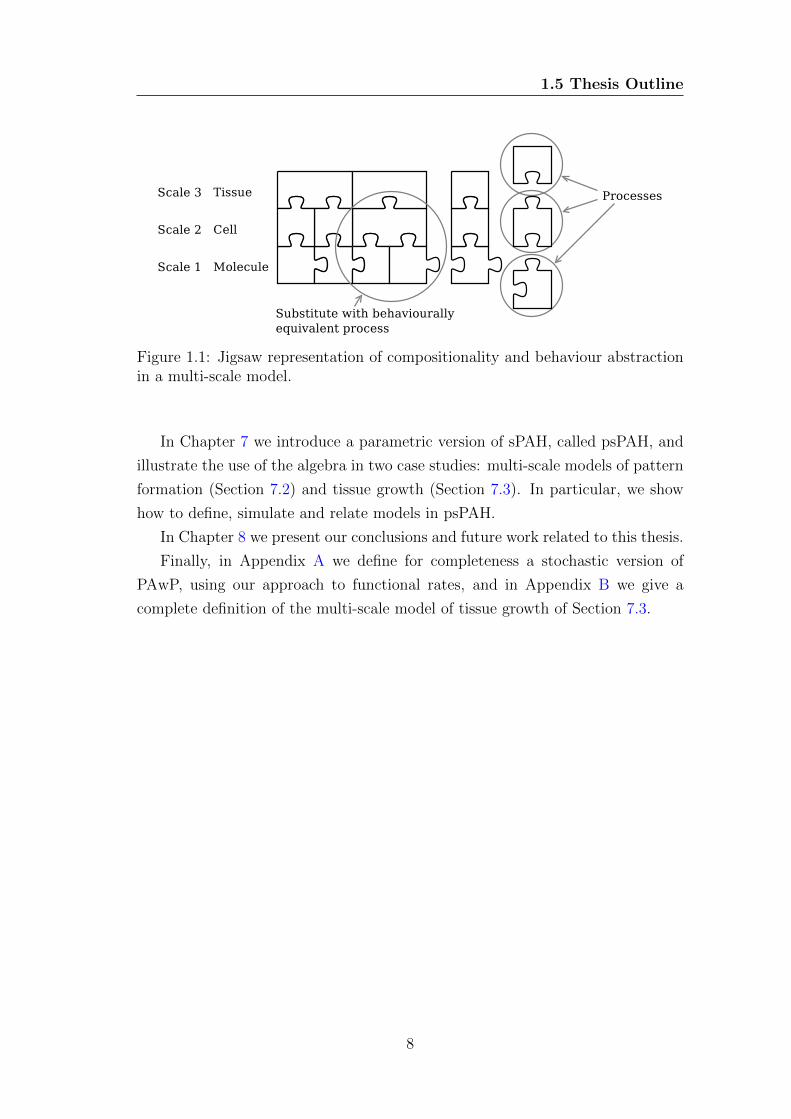
1.1 Jigsaw representation of compositionality and behaviour abstrac-
tion in a multi-scale model. . . . . . . . . . . . . . . . . . . . . . 8
2.1 Example of a CTMC. Numbers on the transitions are exponential
rates. . . . . . . . . . . . . . . . . . . . . . . . . . . . . . . . . . . 20
2.2 Illustration of the concept of levels of concentration. . . . . . . . . 21
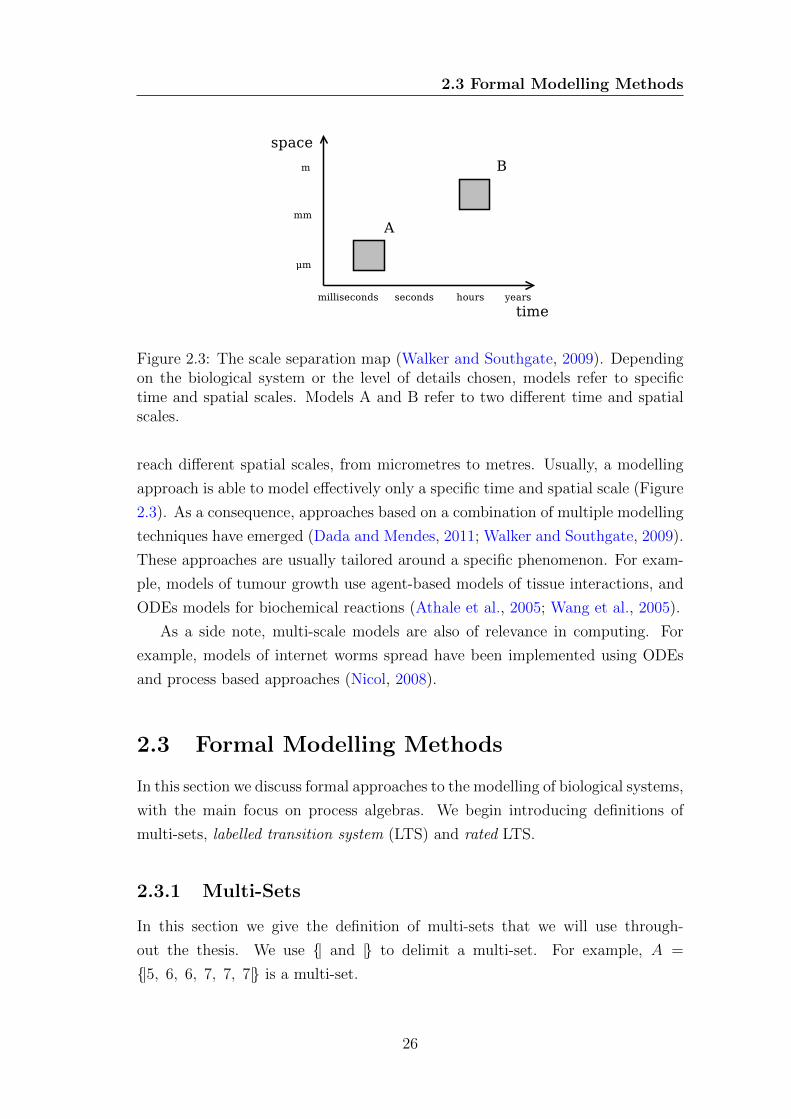
2.3 The scale separation map (Walker and Southgate, 2009). Depend-
ing on the biological system or the level of details chosen, models
refer to specific time and spatial scales. Models A and B refer to
two different time and spatial scales. . . . . . . . . . . . . . . . . 26
2.4 a) Example of a labelled transition system. b) Example of a rated
labelled transition system. . . . . . . . . . . . . . . . . . . . . . . 28
3.1 Semantics of a simple process algebra with multi-way synchronisa-
tion. . . . . . . . . . . . . . . . . . . . . . . . . . . . . . . . . . . 39
3.2 Biochemical reactions and transport between three regions in space. 40
3.3 Explicit modelling of empty space. Every region in space has its
associated process, even if it is empty space. . . . . . . . . . . . . 44
3.4 Graphical representation of process Empty1. . . . . . . . . . . . . 45
3.5 Implicit modelling of empty space on a line. Each region has a
position identified by a natural number. . . . . . . . . . . . . . . . 47
3.6 Stochastic semantics of a simple process algebra. . . . . . . . . . . 53
3.7 Semantics for the evaluation of functional rates. . . . . . . . . . . 56
3.8 Example of a derivation for a valid evaluation of a functional rate. 57
3.9 Semantics of parametric simple process algebra, part one of two. . 69
3.10 Semantics of parametric simple process algebra, part two of two.
Operations on the right hand side of rules are evaluated. . . . . . 70
x
LIST OF FIGURES
4.1 Tissue infection at different abstraction levels: on the left, cellular
scale; centre: molecular scale; on the right: tissue scale. . . . . . . 76
4.2 Interactions between scales. Only if the concentration of a cer-
tain molecule (molecular scale) is high, then a cell can duplicate
(cellular scale). . . . . . . . . . . . . . . . . . . . . . . . . . . . . 77
4.3 Dependencies between scales. Cellular events such as death and
duplication (cellular scale), imply changes in concentration of molecules
(molecular scale) inside the cells. . . . . . . . . . . . . . . . . . . 77
4.4 Example of a threshold definition problem in simple process alge-
bra. . . . . . . . . . . . . . . . . . . . . . . . . . . . . . . . . . . 78
4.5 Reachable states and transitions generated by the example in Sec-
tion 4.2.2. Squares are intermediate states, i.e. states that precede
transitions labelled by actions with priority higher than 1. Auto
transitions (actions move or absorb in states from 1 to 9) are not
shown. . . . . . . . . . . . . . . . . . . . . . . . . . . . . . . . . . 86
4.6 Graphical representation of processes Empty1 and NA1. . . . . . 89
5.1 Semantics of process algebra with hooks. Union of multi-sets is
denoted by ∪ and sum of multi-sets is denoted by ]. . . . . . . . 95
5.2 Reachable states and transitions generated by the example in Sec-
tion 5.1.2. . . . . . . . . . . . . . . . . . . . . . . . . . . . . . . . 103
5.3 Graphical representation of processes NA1 and Empty1. . . . . . . 105
5.4 Two approaches to the use of actions in process algebra in a multi-
scale setting. . . . . . . . . . . . . . . . . . . . . . . . . . . . . . 106
5.5 Stochastic semantics of process algebra with hooks. Union of
multi-sets is denoted by ∪, while sum of multi-sets is denoted by ]. 110
5.6 Rated derivation graph generated by the example in Section 5.2.3. 119
6.1 Two biological systems, if observed at different scales, can present
distinct or analogous behaviour. . . . . . . . . . . . . . . . . . . . 125
6.2 Filtered derivation graphs of the example in this section. a) if ra =
rd, the transition systems are T-isomorphic. b) if rd = ra + re = r
the transition systems are Markovian T-bisimilar. . . . . . . . . . 129
7.1 Semantics of parametric stochastic process algebra with hooks.
Other inference rules are as in Figure 5.5. . . . . . . . . . . . . . . 153
xi
LIST OF FIGURES
7.2 The French Flag Model implemented with partial differential equa-
tions. In the picture, two concentration thresholds divide the space
into three regions. . . . . . . . . . . . . . . . . . . . . . . . . . . . 154
7.3 Discretisation of the space of the French Flag Model into 20 re-
gions. The variable M(i) indicates the concentration of M at
region 1. . . . . . . . . . . . . . . . . . . . . . . . . . . . . . . . . 155
7.4 Agent definitions of processesM(i, w), T (i, z, w), TA(i) and TB(i),
from the multi-scale model of pattern formation. . . . . . . . . . . 156
7.5 Example of simulations of the process algebra with hooks French
Flag Model. On the left: commitments of regions to cell speciali-
sations after 6 seconds. On the right: concentration levels after 6
seconds of the same simulation runs. Top row is the initial condition.159
7.6 Two extensions of the psPAH French Flag Model. In the first
extension, top, two species A and B are added. In the second
extension, bottom, species C is added. . . . . . . . . . . . . . . . 160
7.7 Rated derivation graphs of model processes A0(n)BC∅B0(n) and
C0(n), with n ∈ R. Parameter n is omitted. . . . . . . . . . . . . 161
7.8 Agent definitions of processes C(i, j, w) and T (i, j), from the multi-
scale model of tissue growth. . . . . . . . . . . . . . . . . . . . . . 166
7.9 Three sample runs with k3 equal to 4, 5 and 6 Molar/s. Black
squares represent regions containing tissue. . . . . . . . . . . . . . 167
7.10 Number of tissue regions with parameter k3 equal to 4, 5 and 6
Molar/s, with 100 simulations for each configuration. In the top
row, all 100 simulations are shown, while in the bottom row average
and standard deviation of the same runs. . . . . . . . . . . . . . . 168
xii

List of Tables
7.1 In this table we illustrate the commitments of the 20 regions of
the French Flag Model over 100 simulations and at different time
points. For each region, counts over the simulations of commit-
ments (A, B or none, i.e. not committed) are given. . . . . . . . . 158
xiii
Chapter 1
Introduction
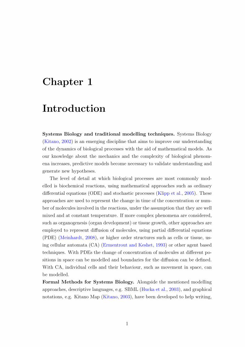
Systems Biology and traditional modelling techniques. Systems Biology
(Kitano, 2002) is an emerging discipline that aims to improve our understanding
of the dynamics of biological processes with the aid of mathematical models. As
our knowledge about the mechanics and the complexity of biological phenom-
ena increases, predictive models become necessary to validate understanding and
generate new hypotheses.
The level of detail at which biological processes are most commonly mod-
elled is biochemical reactions, using mathematical approaches such as ordinary
differential equations (ODE) and stochastic processes (Klipp et al., 2005). These
approaches are used to represent the change in time of the concentration or num-
ber of molecules involved in the reactions, under the assumption that they are well
mixed and at constant temperature. If more complex phenomena are considered,
such as organogenesis (organ development) or tissue growth, other approaches are
employed to represent diffusion of molecules, using partial differential equations
(PDE) (Meinhardt, 2008), or higher order structures such as cells or tissue, us-
ing cellular automata (CA) (Ermentrout and Keshet, 1993) or other agent based
techniques. With PDEs the change of concentration of molecules at different po-
sitions in space can be modelled and boundaries for the diffusion can be defined.
With CA, individual cells and their behaviour, such as movement in space, can
be modelled.
Formal Methods for Systems Biology. Alongside the mentioned modelling
approaches, descriptive languages, e.g. SBML (Hucka et al., 2003), and graphical
notations, e.g. Kitano Map (Kitano, 2003), have been developed to help writing,
1
maintaining and sharing models. This is achieved with unambiguous and de-
scriptive definitions of components and interactions within a model. In addition,
formalisms from the field of computer science have been proposed not only to pro-
vide an unambiguous definition of biological phenomena, but also to improve the
overall modelling approach. They are characterised by being executable, i.e. they
can produce behaviour according to one or more associated semantics. Most im-
portantly, both the syntax and semantics of these formalisms are mathematically
well defined, creating a mathematical framework where formal reasoning between
syntax and semantics is possible. Some of the most successful formalisms are pro-
cess algebras and other calculi (Bortolussi, 2006; Ciocchetta and Hillston, 2009;
Hillston, 1996; Priami and Quaglia, 2005), rewriting rules (Blinov et al., 2004;
Danos et al., 2007) or programming languages (Calzone et al., 2006; Pedersen
and Plotkin, 2008).
Process Algebra for Systems Biology. Process algebras are a family of calculi
developed to represent and analyse formally the behaviour of concurrent systems,
such as programs on a computer or computers in a network (Hoare, 1985; Milner,
1989). They have been shown to be one of the most promising approaches to
the formalisation of biological systems, because of the deep analogies that exist
between concurrent agent interactions and biochemical reactions (Regev et al.,
2001). In particular, process algebra provides:
• a formalisation of biological systems, where biological entities are repre-
sented by processes and biological events are represented by actions that
the processes can perform asynchronously or synchronously. Synchronisa-
tion can be binary, where exactly two processes participate to an action, or
multi-way, where two or more processes participate to an action;
• compositionality, i.e. the possibility of constructing a system as the sum of
its constituent components. This is represented as a cooperation or parallel
composition of processes;
• well established techniques to reason about behaviour. In particular, a
theory of relations based on behaviour, that allows systems to be compared
or part of a system to be abstracted with other parts that are behaviourally
equivalent;
2
• multiple semantics can be derived automatically from a model definition,
which allow for complementary analysis techniques such as ordinary differ-
ential equations, stochastic simulation or continuous time Markov chains.
The development and application of process algebra for biology has usually
been aimed at modelling biochemical reactions and compartments. Specifically, it
has involved the modelling of a single level of detail, whether this is biochemistry
(Calder et al., 2006a; Ciocchetta and Hillston, 2009; Priami and Quaglia, 2005;
Priami et al., 2001) or membrane (Cardelli, 2005). In an exception, multiple
levels of detail are modelled with a single process algebra in Bioambients (Regev
et al., 2004), where biochemistry and modifications of membranes, and so spatial
organisation, are considered.
Multi-scale modelling. More recently there has been a growing interest in
combining different levels of detail of biological phenomena into single multi-
scale models that represent both biochemical details and higher order structures.
This is a necessary step to achieve a complete understanding of the emerging be-
haviour in a complex biological phenomenon. Model construction follows mainly
two approaches: bottom-up and top-down. The former begins from identifying
elementary parts, such as molecules, and aims at explaining more complex phe-
nomena as the emergent behaviour of its components. The latter begins instead
from reproducing observed phenomena and then adds internal details, attempt-
ing to recreate governing mechanisms. Different mathematical approaches are
often considered for different scales and integrated into a multi-scale model tai-
lored around a specific biological problem (Dada and Mendes, 2011; Walker and
Southgate, 2009; Walker et al., 2008). As a consequence, composition and com-
parison of two multi-scale models is often very difficult.
It has been proposed (Noble, 2006) that new, more flexible modelling tech-
niques should allow for a middle-out approach. This means that one begins
studying, and so modelling, a biological phenomenon from any level of detail or
spatial scale and, in a second stage, extending its study and so its model ei-
ther up scale, integrating with other components, or down scale, adding more
internal details. To our knowledge, no formal approach has been proposed that
specifically addresses the problem of integrating multiple scales under the same
mathematical framework and that has the flexibility of treating different scales
as the same formal objects.
3
1.1 Thesis Statement
Process algebra as ‘middle-out’ approach. In this thesis we propose that
process algebra is a perfect candidate as a middle-out approach for multi-scale
modelling. In particular, its natural support of compositionality and its abstrac-
tion mechanisms can provide the required flexibility that writing and composing
multi-scale models require. This leads us to our thesis statement.
1.1 Thesis Statement
There is currently a need for a flexible and compositional modelling approach that
supports the integration of multiple scales, to aid the understanding of complex
biological phenomena such as organogenesis and tumour growth.
We propose that process algebra is a perfect candidate, because of its natural
support of compositionality and its abstraction mechanisms.
We demonstrate this by developing and applying a process algebra dedicated
to the multi-scale modelling of biological systems, after having explored the lim-
itations of current process algebraic approaches.
1.2 The Choice of Multi-Way Synchronisation
In this thesis we consider mainly process algebras with multi-way synchronisation.
Our choice of multi-way over binary synchronisation is motivated as follows:
• it allows one to model biochemical reactions with any number of reactants
and products with a single action, and so atomically (Calder and Hillston,
2009). Moreover, a rate based on one of a variety of kinetic laws (Segel,
1993) can be associated to that action. In general, kinetic laws approximate
sequences of reactions and are employed when it is difficult to measure rates
of some of those reactions in biological experiments;
• it is more amenable for a multi-scale scenario, where multiple scales can be
affected by the same event at the same time.
1.3 Contributions
The main contributions of this thesis are:
4
1.4 Publications
• the definition of process algebra with hooks, a novel process algebra designed
for multi-scale modelling of biological systems. Its main features are: ex-
plicit modelling of scales and interactions within and between scales; use
of composed actions in a multi-way synchronisation setting; a vertical co-
operation operator in addition to the standard cooperation operator for
composition of processes; a stochastic semantics based on functional rates;
• the definition of a functional rate semantics for process algebras based on
biological principles, where actions can be rated only if closed, i.e. only if
all the expected participants to that action synchronise;
• an investigation of the use of a simple process algebra and a process al-
gebra with action priorities in the multi-scale scenario. This investigation
highlights drawbacks that are addressed by process algebra with hooks;
• the definition of three congruence relations to relate and substitute pro-
cess algebra with hooks processes. They relate processes by their structure
(isomorphism), by their structure with focus on a specified scale ((T,Γ)-
isomorphism) and by their spatial and temporal behaviour at a specified
scale (Markovian (T,Γ)-bisimulation). The proof of congruence for (T,Γ)-
isomorphism and Markovian (T,Γ)-bisimulation is possible because of the
concept of closed actions introduced with our definition of functional rates;
• the illustration of use of process algebra with hooks to model, simulate and
relate multi-scale models of pattern formation and tissue growth.
1.4 Publications
Investigation of the thesis and related topics led to the following publications:
• A. Degasperi and M. Calder. Multi-Scale Modelling of Biological Systems in
Process Algebra with Multi-Way Synchronisation. CMSB 2011, to appear
in ACM Digital Library, 2011;
• A. Degasperi and M. Calder. Process Algebra with Hooks for Models of
Pattern Formation. CS2Bio2010, ENTCS 268, pages 31-47, Elsevier, 2010;
5
1.5 Thesis Outline
• A. Degasperi and M. Calder. Relating PDEs in Cylindrical Coordinates and
CTMCs with Levels of Concentration. CS2Bio2010, ENTCS 268, pages 49-
59, Elsevier, 2010;
• A. Degasperi and M. Calder. On the Formalisation of Gradient Diffusion
Models of Biological Systems. PASTA Workshop 2009, unreviewed, 2009;
• F. Ciocchetta, A. Degasperi, J. Hillston, M. Calder. Some investigations
concerning the CTMC and the ODE model derived from Bio-PEPA. FBTC
2008, ENTCS 229(1), pages 145-163, Elsevier, 2009.
1.5 Thesis Outline
The thesis is organised as follows. After discussing background material in Chap-
ter 2, we investigate the use of a simple process algebra with multi-way synchro-
nisation (SPA) to model a single spatial scale in Chapter 3. In Chapter 4 we move
the focus on to multi-scale modelling showing how SPA is not suited to model
desired inter-scale interactions and how a process algebra with priorities (PAwP)
can be used as well as the drawbacks of this approach. Building on the previ-
ous chapters, we propose process algebra with hooks (PAH) in Chapter 5 which
presents the advantages of PAwP with respect to SPA, without its drawbacks. In
Chapter 6 we continue the characterisation of PAH introducing three equivalence
relations, while in Chapter 7 we apply a parametric stochastic version of PAH to
the modelling of two case studies. Conclusions and future work are in Chapter 8.
We now present a more detailed overview of the thesis.
In Chapter 2 we cover background material, from useful biological concepts
in Section 2.1, to a survey of traditional modelling approaches in Section 2.2, and
a discussion of formal methods for systems biology with focus on process algebra
in Section 2.3.
In Chapter 3 we show how a simple process algebra with multi-way synchro-
nisation (SPA) can be used to model a single spatial scale. First, we introduce
a non stochastic version of the semantics (Section 3.1) and propose examples of
modelling biochemistry and tissue growth (Sections 3.1.1 and 3.1.2). Second,
we consider a stochastic semantics for simple process algebra (sSPA) based on
functional rates (Section 3.2). An example of the application of stochastic sim-
ple process algebra is in Sections 3.2.5. To conclude the chapter on modelling a
6
1.5 Thesis Outline
single scale, we propose a parametric process algebra (pSPA) that makes model
definition more compact (Section 3.3). Examples are given in Sections 3.3.1 and
3.3.2.
In Chapter 4 we introduce the concept of interactions between scales (Section
4.1) and discuss how SPA is not ideal to model such interactions (Section 4.1.1).
Then, we introduce a process algebra with priority of actions (PAwP, in Section
4.2). Actions with low priority are considered local and represent the behaviour
of a single scale. Actions with high priority are considered inter-scale interrupts,
i.e. signals operating between scales. We illustrate how this algebra can be
employed successfully to the multi scale modelling of biological systems with
examples (Sections 4.2.3 and 4.2.2). Finally, we highlight some drawbacks of
the use of action priorities: the creation of additional, intermediate, biologically
meaningless states; the lack of control by the modeller when multiple inter-scale
signals happen at the same time; the lack of explicit syntactic elements that could
unambiguously represent scales and actions operating within and between scales
and that could improve the overall compositionality of the algebra.
In Chapter 5 we introduce process algebra with hooks (PAH, in Section 5.1),
which is designed for multi scale modelling of biological systems and which ad-
dresses the drawbacks identified in PAwP. In particular, instead of using separate
actions for intra and inter-scale interactions, composed actions are used. This
means that a single composed action can perform both interactions within and
between scales. Examples are presented in Sections 5.1.3 and 5.1.2. A compari-
son between PAwP and PAH is given in Section 5.1.4. Stochastic process algebra
with hooks (sPAH) is introduced in Section 5.2 with examples in Sections 5.2.4
and 5.2.3.
In Chapter 6 we continue the characterisation of sPAH, defining congruences
on processes, which can relate processes with equivalent behaviour at a specified
scale, abstracting away as much as possible from other scales. Although at a
certain scale the behaviour of biological systems can be different, e.g. different
biochemical networks are present, at a higher or lower scale behaviour could be
analogous under a certain notion of equivalence, e.g. in both cases cells prolifer-
ate and die at the same rate. Equivalence relations can also be used to substitute
parts within a model with equivalent and possibly less complex alternatives (Fig-
ure 1.1).
7
1.5 Thesis Outline
Figure 1.1: Jigsaw representation of compositionality and behaviour abstractionin a multi-scale model.
In Chapter 7 we introduce a parametric version of sPAH, called psPAH, and
illustrate the use of the algebra in two case studies: multi-scale models of pattern
formation (Section 7.2) and tissue growth (Section 7.3). In particular, we show
how to define, simulate and relate models in psPAH.
In Chapter 8 we present our conclusions and future work related to this thesis.
Finally, in Appendix A we define for completeness a stochastic version of
PAwP, using our approach to functional rates, and in Appendix B we give a
complete definition of the multi-scale model of tissue growth of Section 7.3.
8
Chapter 2
Background
In this chapter we survey useful biological concepts in Section 2.1, traditional
modelling approaches in Section 2.2 and discuss formal methods for systems bi-
ology with focus on process algebra in Section 2.3.
2.1 Biological Concepts
In this section we cover concepts useful to the understanding of the biology in
the thesis. Our references for this section are (Nelson and Cox, 2004) and (Klipp
et al., 2005).
2.1.1 The Complexity of Organisms
Every organism, whether it is an animal, a plant or a bacterium, consists of
biochemical molecules, which participate in complex interactions and collective
behaviour. These molecules have highly specific functions and can be organised
in higher order structures, such as membranes, cells, tissues or organs. Physical
forces and chemical reactions allow organisms to function as dynamic entities,
able to sense the environment they are in and respond accordingly. In this in-
troduction, we discuss some of the principles that allow cells to make decisions,
with focus on pattern formation in the development of organisms.
We begin by explaining what proteins are and how they can interact to cre-
ate metabolic and signalling networks. Then we overview mechanisms of cell
differentiation and memory.
9
2.1 Biological Concepts
2.1.2 Proteins
In order to explain what proteins are, we briefly introduce the central dogma of
molecular biology. DNA (deoxyribonucleic acid) is the molecule, in every cell,
that contains information about how to construct (synthesise) proteins. This
information is coded as a sequence of bases: adenine, thymine, guanine and
cytosine. When a protein needs to be built, a process called transcription copies
the necessary sequence of bases from the DNA to a strand of RNA (ribonucleic
acid). Then, during translation, the RNA binds to a molecule called ribosome
and the information present in the RNA is used to construct a chain of amino
acids. After a chain of amino acids is formed, this chain folds, thanks to bonds
and forces acting on it, leading to the final shape of the protein.
A gene is a sequence of DNA which encodes one or more proteins or a strand
of RNA that has a function in the cell or organism. A gene is said to be expressed
if its sequence of DNA is transcribed and, possibly, translated into a protein.
Proteins fulfil numerous functions in the cell, from being just part of the
cellular structure to having roles in the metabolism of the cell or in the delivery
of signals. The main characteristic of proteins that enables them to have so
many different functions is their ability to bind to other molecules specifically
and tightly. The regions in the protein where other molecules may bind are
called binding sites. These regions are defined by their shape and by the chemical
properties that surround them, allowing only very specific molecules to bind.
Proteins can also bind to other proteins or be integrated into membranes. When
a protein binds to another molecule, it can also change some of its properties and
abilities to bind.
Enzymes. An enzyme is a protein whose role is to catalyse, i.e. to accelerate,
a biochemical reaction. Enzymes allow reactions that are normally unfavourable
in nature to take place, lowering their activation energy. We will call reactants
the molecules that take part in catalysed reactions and products the molecules
that are generated. Usually enzymes only catalyse very specific reactions.
2.1.3 Metabolic and Signalling Pathways
The metabolism of a cell is a highly organised process, that involves thousands
of reactions that are catalysed by enzymes and whose ultimate goal is to pro-
vide everything the cell needs to survive and reproduce. Metabolism provides
10
2.1 Biological Concepts
energy and material for building and maintaining the cell. Metabolic pathways
are networks of biochemical interactions that involve mainly mass and energy
transfer.
On the other hand, a signalling pathway is a sequence of biochemical inter-
actions that leads to the transmission of external signals from outside to inside
the cell and to the movement of information inside the cell. Examples of signals
are hormones, pheromones, heat, cold, light or even the appearance or concen-
tration change of substances such as glucose or potassium or calcium ions. The
interpretation of these external signals triggers the cell response.
2.1.4 Biological Mechanisms of Cell Differentiation and
Decision Making
The genome, i.e. the set of all genes of an organism, is normally identical in every
cell. Cell differentiation, and so specialisation of function, is achieved by selecting
different genes to be expressed in individual cells, while the genetic information
contained in all of them is mostly identical. Gene selection controls four essential
processes of a cell: cell proliferation, cell specialisation, cell interactions and cell
movements.
Many biological processes are transient, i.e. changes in gene expression are
temporary. For example, a response to an external signal can activate genes as a
response. When the signal is gone, the response ceases.
A stable choice of gene expressions is possible because of cell memory. Which
genes are expressed depends on the past, along with the present environment.
Memory is essential for the creation of organised tissues and for the stable main-
tenance of cell specialisation.
Although other mechanisms are possible, cell differentiation is mainly achieved
by sensing concentration levels of specific proteins. Even a single protein, present
in high concentration, can activate entire pathways and transcription circuits,
deciding irreversibly the fate of the cell it is in. Multiple thresholds (for example
high, medium and low concentration) are not uncommon.
Thus, if the concentration of a protein in a cell can determine its differen-
tiation, two originally identical cells with different fates must have reached a
different concentration level for that protein at a key moment in time, when the
selection took place. How this different concentration level arises is probably the
11
2.2 Traditional Modelling Methods
most important question addressed by the field of Developmental Biology. In
general, this phenomenon involves a notion of spatial location.
Using memory, cells can remember their position, referred to as positional
value. During organism development, the memorisation of position is often an
intermediate step between non-specialised and specialised cells.
A group of cells can be influenced by a signal coming from neighbouring cells,
called an inductive signal, driving one or more of the members of the group into
a different developmental pathway. This process is called inductive interaction
and it consists of a signal limited in time and space. An inductive signal can
be long range, e.g. highly diffusible molecules, or short range, e.g. cell-to-cell
interactions. Inductive signal molecules are often referred to as morphogens.
2.2 Traditional Modelling Methods
Biological interactions can be modelled and studied at different levels of detail.
It is possible to concentrate on the properties of individual reactions as well as
studying the system as a whole. In this section, we consider models of biochemical
reactions, as this is the most popular level of detail.
The main mathematical approaches to quantitative analysis we discuss in
this section are: Ordinary Differential Equations (ODEs), Stochastic Simulation
Algorithm (SSA) based on the Chemical Master Equation (CME), Continuous
Markov Chain with levels (CTMCs with levels) and Reaction-Diffusion Equations
(RDE).
2.2.1 ODE: The Law of Mass Action
ODEs are the most common way of modelling chemical or biochemical inter-
actions. They express the rate of change in time of the concentration of the
participants of a biochemical reaction in an environment where molecules are
well-mixed. Each biochemical reaction is associated with a rate of change, called
the velocity of the reaction. Velocities are usually dependent on the concentration
of the molecules that are involved in the modelled reaction. Often, a velocity is
expressed in terms of a kinetic law, i.e. an equation that expresses the dynam-
ics of multiple biochemical interactions at a time. A kinetic law may take into
12
2.2 Traditional Modelling Methods
account which molecules can be measured in a biological experiment in order to
determine the value of constant parameters (Segel, 1993).
The key characteristic of the ODE approach is the fact that it shows the
most likely behaviour of the system, assuming continuous concentrations, i.e. an
infinite number of interacting molecules.
A common kinetic law is the law of mass action, introduced in the 19th century
(Guldberg and Waage, 1879). It states that the rate at which a species is produced
or consumed by a reaction is proportional to the amount of reactants and the
stoichiometry, i.e. how many copies of a reactant are involved in the reaction.
For example, the velocity of the reaction
S1 + S2 � 2P
can be formulated as
v = v+ − v− = k+ · [S1] · [S2]− k− · [P]2
where S1, S2 and P are molecular species, v is the velocity, v+ is the velocity of
only the forward reaction, v− is the velocity of the backward reaction and k+ and
k− are the proportionality factors, called kinetics or rate constants. The symbol
[·] denotes the concentration of the species, usually expressed in moles per litre
(mol/L) or molar (M). We use bold-capital font for molecules. The dynamics
of the concentrations of the species can be described by Ordinary Differential
Equations (ODEs) for example the equations for the reactions above are given
by:
d[S1]
dt=d[S2]
dt= −v
d[P]
dt= 2v
The value of the concentrations of S1, S2 and P through time are obtained
by integration of these ODEs.
2.2.2 Generalised Mass Action
In this section we generalise and formalise the concepts we introduced in the
previous section.
13
2.2 Traditional Modelling Methods
Modelling intracellular dynamics in a quantitative way is concerned with
the estimation through time of the number of molecules of n different species
S1, . . . ,Sn, which can interact according to m biochemical reactions Rj. In gen-
eral, a biochemical reaction Rj can be formalised as follows:
Rj : κj1Sp(j,1) + κj2Sp(j,2) + ...+ κjLjSp(j,Lj)kj−→ κjLj+1Sp(j,Lj+1) + ...+ κjTjSp(j,Tj)
where Lj is the number of reactants and Tj is the number of reactants and prod-
ucts in Rj, κjz is the stoichiometric coefficient of the reactant species Sp(j,z),
Kj=∑Lj
z=1 κjz denotes the molecularity of the reaction Rj and the index p(j, z)
selects those Si participating in Rj. The stoichiometric coefficient indicates how
many copies of a species participate to a reaction.
Assuming a constant temperature and that diffusion in the cell is fast, so that
we can assume a homogeneously distributed mixture in a fixed volume V , the
General Mass Action (GMA) model of the system can be defined by n ordinary
differential equations (ODEs) as follows:
d[Si]
dt=
m∑j=1
djikj
Lj∏z=1
[Sp(j,z)]κjz i = 1, 2, ..., n (2.1)
where the kjs are rate constants, dji denotes the change in molecules of Si resulting
from a single Rj reaction and m is the number of reactions. Symbol [Si] is the
concentration of the species Si.
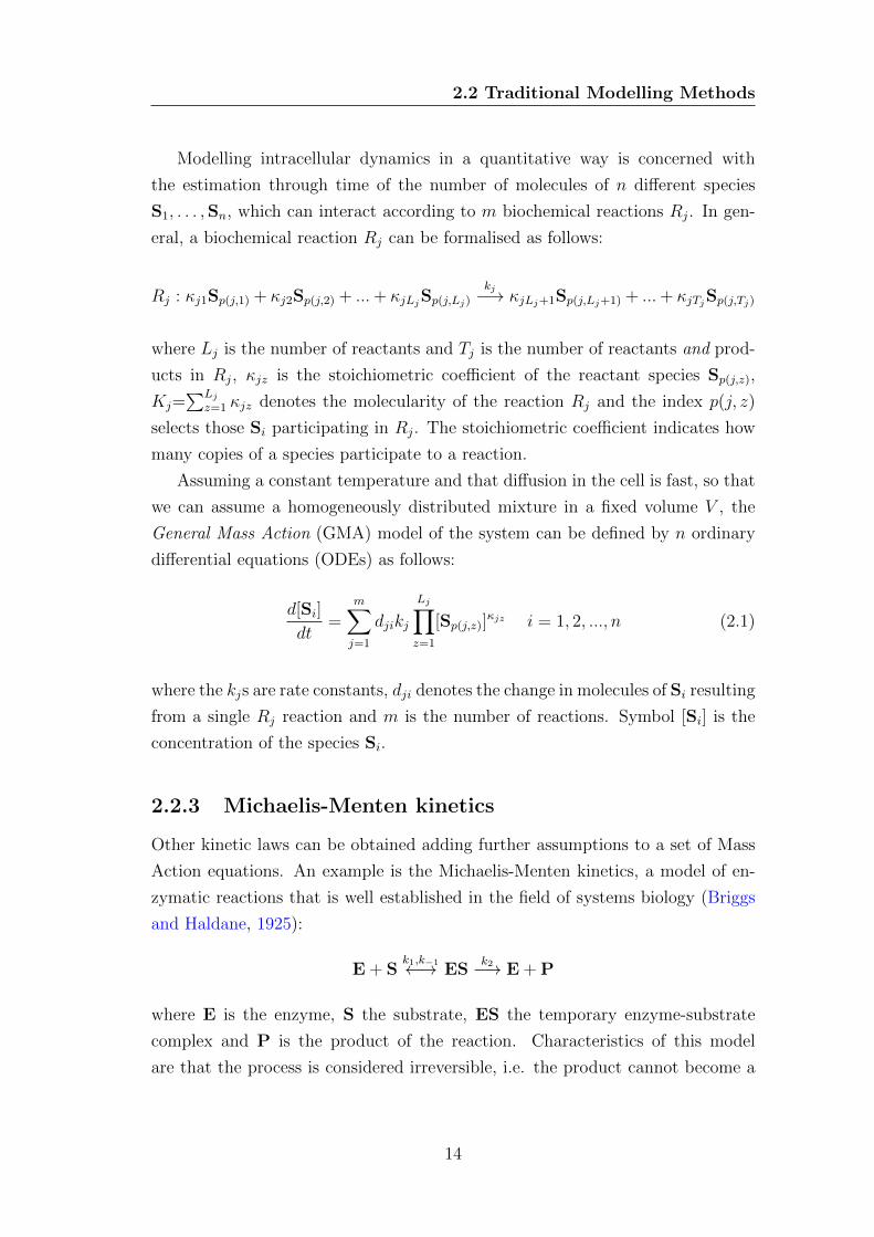
2.2.3 Michaelis-Menten kinetics
Other kinetic laws can be obtained adding further assumptions to a set of Mass
Action equations. An example is the Michaelis-Menten kinetics, a model of en-
zymatic reactions that is well established in the field of systems biology (Briggs
and Haldane, 1925):
E + Sk1,k−1←→ ES
k2−→ E + P
where E is the enzyme, S the substrate, ES the temporary enzyme-substrate
complex and P is the product of the reaction. Characteristics of this model
are that the process is considered irreversible, i.e. the product cannot become a
14
2.2 Traditional Modelling Methods
substrate, and the enzyme is not affected by the reactions and can be used again
after it leaves the substrate or the product.
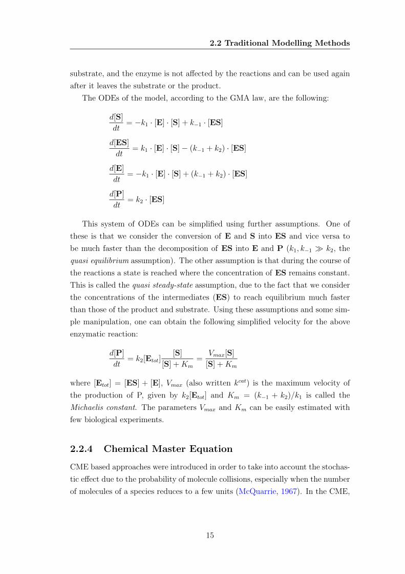
The ODEs of the model, according to the GMA law, are the following:
d[S]
dt= −k1 · [E] · [S] + k−1 · [ES]
d[ES]
dt= k1 · [E] · [S]− (k−1 + k2) · [ES]
d[E]
dt= −k1 · [E] · [S] + (k−1 + k2) · [ES]
d[P]
dt= k2 · [ES]
This system of ODEs can be simplified using further assumptions. One of
these is that we consider the conversion of E and S into ES and vice versa to
be much faster than the decomposition of ES into E and P (k1, k−1 � k2, the
quasi equilibrium assumption). The other assumption is that during the course of
the reactions a state is reached where the concentration of ES remains constant.
This is called the quasi steady-state assumption, due to the fact that we consider
the concentrations of the intermediates (ES) to reach equilibrium much faster
than those of the product and substrate. Using these assumptions and some sim-
ple manipulation, one can obtain the following simplified velocity for the above
enzymatic reaction:
d[P]
dt= k2[Etot]
[S]
[S] +Km
=Vmax[S]
[S] +Km
where [Etot] = [ES] + [E], Vmax (also written kcat) is the maximum velocity of
the production of P, given by k2[Etot] and Km = (k−1 + k2)/k1 is called the
Michaelis constant. The parameters Vmax and Km can be easily estimated with
few biological experiments.
2.2.4 Chemical Master Equation
CME based approaches were introduced in order to take into account the stochas-
tic effect due to the probability of molecule collisions, especially when the number
of molecules of a species reduces to a few units (McQuarrie, 1967). In the CME,
15
2.2 Traditional Modelling Methods
each molecule of the system is modelled and has a probability to react, thus al-
lowing modelling of likelihood of states of the system. A state is a snapshot of
the number of molecules for each species at a given time. This is at the price of
a sometimes problematic computational complexity.
In CME based approaches we wish to determine for each molecular species Si
the probability P (#Si(t) = si) that at time t there are si molecules (with #Si
denoting the number of molecules of the species Si). For n molecular species, let
s ∈ Nn denote the n dimensional state vector. The vectors dj ∈ Zn are the step
changes occurring for elementary reactions indexed by j. If S is an n dimensional
variable, we write P (#S = s) as Ps(t). In order to describe the changes in random
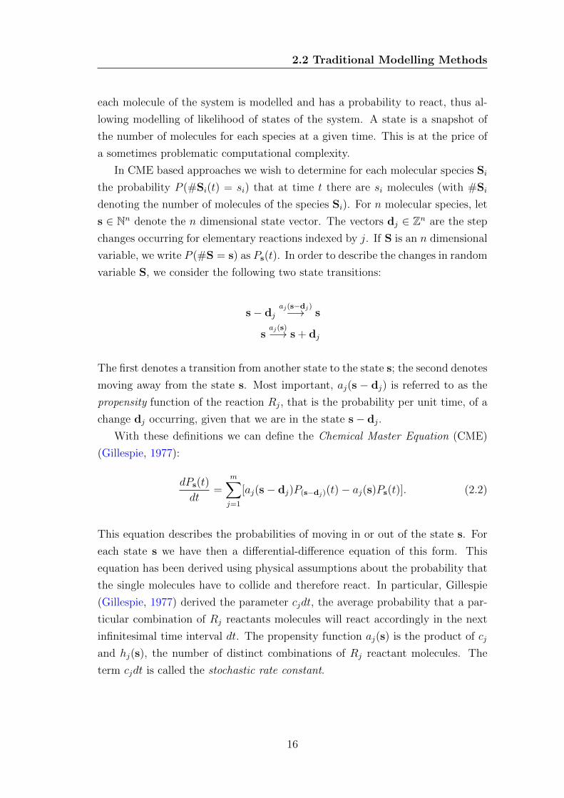
variable S, we consider the following two state transitions:
s− djaj(s−dj)−→ s
saj(s)−→ s + dj
The first denotes a transition from another state to the state s; the second denotes
moving away from the state s. Most important, aj(s − dj) is referred to as the
propensity function of the reaction Rj, that is the probability per unit time, of a
change dj occurring, given that we are in the state s− dj.
With these definitions we can define the Chemical Master Equation (CME)
(Gillespie, 1977):
dPs(t)
dt=
m∑j=1
[aj(s− dj)P(s−dj)(t)− aj(s)Ps(t)]. (2.2)
This equation describes the probabilities of moving in or out of the state s. For
each state s we have then a differential-difference equation of this form. This
equation has been derived using physical assumptions about the probability that
the single molecules have to collide and therefore react. In particular, Gillespie
(Gillespie, 1977) derived the parameter cjdt, the average probability that a par-
ticular combination of Rj reactants molecules will react accordingly in the next
infinitesimal time interval dt. The propensity function aj(s) is the product of cj
and hj(s), the number of distinct combinations of Rj reactant molecules. The
term cjdt is called the stochastic rate constant.
16
2.2 Traditional Modelling Methods
It is interesting to remark that it has been proved there is a correspondence
between cj and the GMA rate constant kj (Wolkenhauer et al., 2004):
cj =
(kj
(NAV )Kj−1
)·Lj∏z=1
(κjz!) (2.3)
where NA is the Avogadro number and V is the cell volume. This allows one to
pass from one method to the other as soon as either cj or kj has been identified
from experimental data.
2.2.5 Stochastic Simulation Algorithm
A major difficulty with the CME is that its analytical solution is usually in-
tractable. For this reason, Gillespie (Gillespie, 1977) developed the Stochastic
Simulation Algorithm (SSA), a Monte Carlo simulation of the CME. A single
simulation represents one exact possible evolution of the system, while a set of
thousands of these simulations can be used to identify a probability function that
is an approximation of the CME.
This algorithm proceeds with a loop in which, at every iteration, two param-
eters are randomly taken from previously defined probability distributions: the
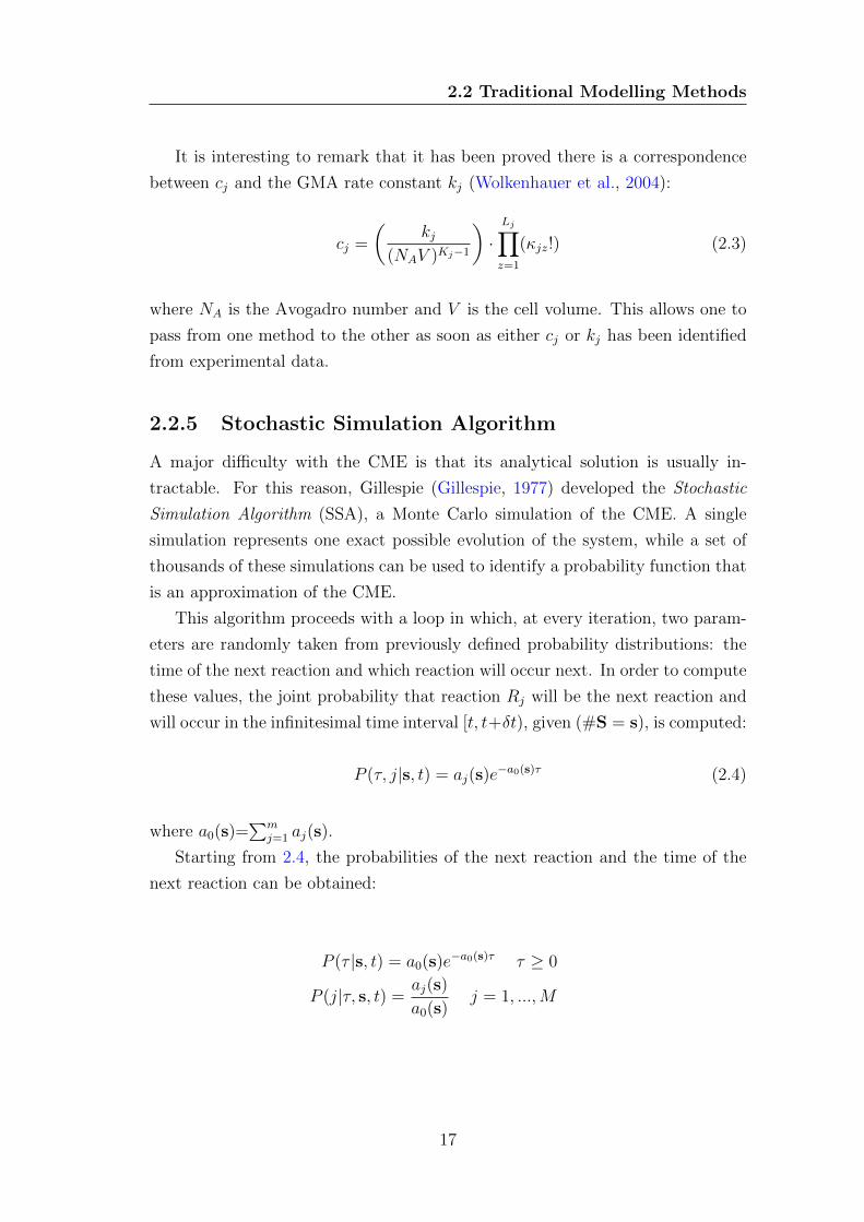
time of the next reaction and which reaction will occur next. In order to compute
these values, the joint probability that reaction Rj will be the next reaction and
will occur in the infinitesimal time interval [t, t+δt), given (#S = s), is computed:
P (τ, j|s, t) = aj(s)e−a0(s)τ (2.4)
where a0(s)=∑m
j=1 aj(s).
Starting from 2.4, the probabilities of the next reaction and the time of the
next reaction can be obtained:
P (τ |s, t) = a0(s)e−a0(s)τ τ ≥ 0
P (j|τ, s, t) =aj(s)
a0(s)j = 1, ...,M
17
2.2 Traditional Modelling Methods
From these distributions, random Monte Carlo samples can be taken using two
uniform random numbers r1 and r2 from [0, 1]. Time delay τ is given by:
τ =1
a0(s)ln
(1
r1
)(2.5)
The index j of the selected reaction is the smallest integer in [1,m] such that
j∑j′=1
aj′(s) > r2a0(s) (2.6)
Once these two values are computed, the system is updated adding the selected
dj to s and τ summed to t.
CME and SSA are very specific to the biochemical context. We now turn our
attention to a more general type of stochastic model: continuous time Markov
chains (CTMCs).
2.2.6 Deterministic and Stochastic Approaches
A deterministic approach to the modelling of biochemical reactions is charac-
terised by producing the most likely behaviour of the system and expressing its
output as the continuous concentration of the biochemical species. In contrast,
a stochastic approach considers the likelihood of alternative behaviours and ex-
presses its output as discrete quantities, such as number of molecules or levels of
concentration.
Deterministic ODE based models are widely used in modelling biochemical
interactions. They represent the most efficient approach, able to model hundreds
of reactions at the same time. However, ODE does not account for randomness or
stochasticity, which are key features of biochemical interactions (McAdams and
Arkin, 1999). When experimental evidence for the modelled systems presents
low variability or all the species in the systems are present in large quantities, we
might consider ODEs to be the most suitable representation. However, even in
systems which exhibit low variability this may be due to high resistance to noise
and some behaviour may be lost with a deterministic approach.
An example of such behaviour is the circadian clock, a biochemical system
that presents oscillations. It has been shown that only stochastic models allow
18
2.2 Traditional Modelling Methods
identification of which interactions are required for the oscillations to resist the
randomness of the interactions (Barkai and Leibler, 2000). Another example can
be found in the repressilator presented here, where experimental data highlights
weak resistance to noise (Elowitz and Leibler, 2000).
In general, a stochastic approach offers a more accurate representation of the
biological interactions under study. However, this type of approach presents the
main drawback of being computationally expensive, thus limiting the size of the
biochemical network that can be analysed.
2.2.7 Continuous Time Markov Chain
Definition 2.1 Continuous time Markov chain. A continuous time Markov
chain (CTMC)(Ross, 1983) is a pair (U,→) where:
• U is a countable set of states;
• → is a set of transitions with →⊆ (U ×R>0×U). The real number associ-
ated with each transition is the rate for the exponential time delay for the
transition to happen.
The set of transitions → can be interpreted as the infinitesimal generator
matrix Q = {qij}, i, j ∈ U , which collects the rates of the transition from state i
to j. The elements qij of the matrix Q are defined as follows:
if i 6= j then qij =
{r if ∃r ∈ R>0, (i, r, j) ∈→0 otherwise
qii = −∑
j 6=i qij
The probability Pij(t) to move from a state i to a state j within a time t is given
by an exponential distribution with rate qij, i.e.
Pij(t) = 1− e−qijt
In the presence of multiple transitions outgoing from a state i, a race condition
is employed. A race condition implies that the transitions outgoing from a state
i are in competition and that the faster transition will be triggered, determining
the next state j. Once this happens a new race starts to determine the successive
19
2.2 Traditional Modelling Methods
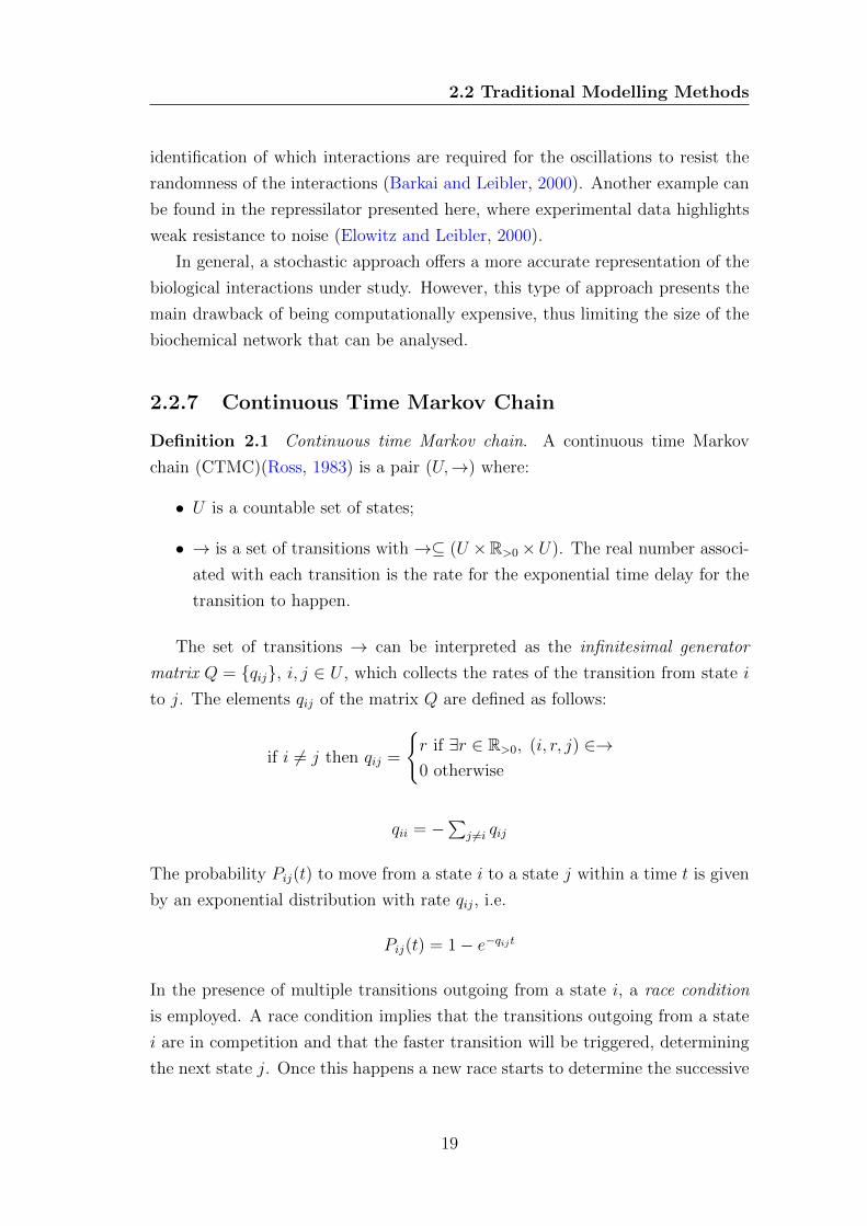
Figure 2.1: Example of a CTMC. Numbers on the transitions are exponentialrates.
state. Because each transition is associated with an exponential time delay, the
time delay to leave i will also be exponentially distributed with a rate equal to
the sum of the rates of the outgoing transitions.
An Example of a CTMC is depicted in Figure 2.1. In this example, U =
{a, b, c} while the infinitesimal generator matrix is given by:
Q =
−2.5 0.5 2
0 −1 1
0.8 0 −0.8
Sampling over a CTMC. Given the initial state u ∈ U of a CTMC, a next
state and a time delay can be sampled in analogy with SSA (Section 2.2.5).
Using qu =∑
j quj and rand1 and rand2 uniform random numbers in [0, 1],
the time delay τ is given by:
τ =1
quln
(1
rand1
)
The index j of the selected reaction is the smallest integer in [1, n] such that
j∑i=1
qui > rand2qu
The sampling can be repeated until no transitions are possible, i.e. an absorbent
state is reached, or until the sum of the time delays reaches a time threshold. A
20
2.2 Traditional Modelling Methods
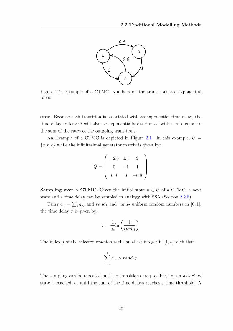
Figure 2.2: Illustration of the concept of levels of concentration.
sequence of samplings forms a trace of the form u, τ1, u1, τ2, u2, . . . , τm, um, also
called a Monte Carlo simulation of the CTMC. A collection of simulations can
be used to estimate the probability density function capturing the likelihood of
the states of the CTMC in time.
In the next section we illustrate how CTMCs can be used to model biochemical
reactions.
2.2.8 CTMC with Levels of Concentration
The CTMC with levels is a family of CTMCs that can be used to model biochemi-
cal species abstracting their concentration with discrete levels. The Markov chains
belonging to this family have a common definition and differ only in the number
of levels used for each species and the amount of concentration represented by
one level. Models of biochemical interactions written in ODEs can be converted
easily into CTMC with levels.
The original idea behind CTMC with levels was to represent signals in a cell,
in terms of high and low concentration of species involved in signalling pathways
(Calder et al., 2006b). It then became evident that an arbitrary number of
levels could be used. Moreover, Kurtz’s Theorem (Kurtz, 1971) provides a strong
theory that links CTMCs with different number of levels with one another and
that relates them to ODE models of the same modelled system.
In Figure 2.2 we illustrate the concept of levels of concentration. Initially, a
preliminary investigation is necessary, in order to identify the maximum concen-
tration M ∈ R+ for each species. Then a number N ∈ N is chosen to divide the
21
2.2 Traditional Modelling Methods
range of values into discrete levels {0, 1, ..., N}. The step size or granularity of
the model is defined as h = M/N and represents the amount of concentration
represented by one level.
A state of a CTMC with levels of concentration is defined as the vector σ =
(〈S1〉, ..., 〈Sn〉). The notation 〈Si〉 indicates the current level of concentration of
the species Si, with 0 ≤ 〈Si〉 ≤ N . An index j is assigned to each biochemical
reaction. The dynamics of the reactions are described by kinetic laws vj, such
as Mass Action or Michaelis-Menten. We consider the case in which each species
has the same step size h.
The rates of the CTMC, used to pass from one state to another, are defined
as follows. Let d[Si]/dt = vj(x,dj) be a kinetic law, Si one of the products, x
the vector of concentrations of reactants and modifiers of reaction j and dj =
(d1,j, ..., dn,j) the vector of the stoichiometric coefficients of reaction Rj. Consider
the following linear approximation:
[Si]t′ ≈ [Si]t + vj(xt,dj) · (t′ − t)
where [Si]t is the concentration of the species Si at time t and t′ − t = ∆t is the
time difference between t′ and t. We can now define the step size of the species
Si as h = [Si]t′ − [Si]t - the difference in concentration between two levels. With
h fixed we can define:
λj =1
∆t=vj(xt,dj)
h
where λj is defined as the rate, or parameter of an exponential distribution
g(t, j) = e−λjt, with mean E[g(t, j)] = 1/λj = ∆t. Since xt = σt · h, λj is
the rate of the reaction j and is a function of the current state σt. A reaction j
brings the current state from σu to σv = σu + dj.
An interesting theoretical result is derived from Kurtz’s Theorem (Kurtz,
1971). It states that, in the limit of a decreasing step size in the CTMC, the
most likely time evolution tends to the ODE simulation. For a more detailed
explanation see (Ciocchetta et al., 2009).
2.2.9 Compartments
Compartments are spatial locations that abstract cells, organelles (e.g. mito-
chondria) or other entities that can contain molecular species and that are char-
acterised by a volume.
22
2.2 Traditional Modelling Methods
Let A be a species inside a compartment Ca with volume Va that can be
transported to another compartment Cb with volume Vb, where it takes the new
name B. This can be represented by the following transport reaction Rt:
Rt : A −→ B
The ODEs for this model are:
v = k[A] Va ·d[A]
dt= −v Vb ·
d[B]
dt= v (2.7)
where v is the velocity of the transport in moles per time unit. The rates of the
corresponding CTMC with levels can be derived as follows. From Equation (2.7),
we can infer the rate λ of the exponential distribution of the time necessary to
transport one level of concentration of A from Ca to Cb.
Consider the following difference equations:
Va ·∆[A]
∆t= −v Vb ·
∆[B]
∆t= v
⇒ Va ·∆〈A〉 · ha
∆t= −v Vb ·
∆〈B〉 · hb∆t
= v
where ∆〈A〉 and ∆〈B〉 are the changes in number of levels of A and B after the
transport of one level of concentration from Ca to Cb. We assume these to be
∆〈A〉 = −1, i.e. A decreases one level and ∆〈B〉 = 1, i.e. B increases one level.
We then obtain:
λ =1
∆t=
v
Vb · hb=
v
Va · ha(2.8)
It is worth noting that Equation (2.8) implies that hb = ha · Va/Vb.
2.2.10 Reaction-Diffusion Equations
So far we have assumed that biochemical reactions happen in a well-mixed en-
vironment. This implies that diffusion of molecules is so fast that whenever
23
2.2 Traditional Modelling Methods
biochemical reactions take place, molecules are immediately rearranged to a well-
mixed solution. However, many processes in biology, such as pattern formation in
development, can be modelled only if diffusion of molecules in space is represented
explicitly.
Modelling diffusions of species S is defined at a macroscopic level by Fick’s
equation, a Partial Differential Equation (PDE) of the form:
∂[S]
∂t= DS∇2[S] (2.9)
where DS is the diffusion coefficient of species S, [S] now represents the concen-
tration density of S at a point in space and ∇2 is the Laplacian operator, which
can be interpreted in different ways, depending on the coordinate system. When
diffusion is considered along with local biochemical interactions, the following
reaction-diffusion equation (RDE) is employed (Berg, 1993; Jones and Sleeman,
1983):
∂[S]
∂t= DS∇2[S]± React (2.10)
where React represents the velocities of other reactions involving species S. In
order to compute the concentration of S in a volume, [S] has to be integrated
in that volume. An example of reaction-diffusion equation in one-dimensional
coordinates is:
∂[S](t, x)
∂t= DS
∂2[S](t, x)
∂x2− kdeg[S](t, x) (2.11)
where x indicates the position and t the time. In order to solve a RDE, initial
conditions and boundary conditions need to be specified. In particular, boundary
conditions are constraints to be applied at the edges of the spatial area considered.
Usually they specify whether the boundaries reflect or absorb the concentration
that reaches the edges. Models defined by reaction-diffusion equations can also
be approximated by a CTMC with levels. In this case, space has to be divided
into regions and the diffusion term of the equations is approximated by the mass
action kinetic law. For details about this procedure see (Erban et al., 2007).
24
2.2 Traditional Modelling Methods
2.2.11 Modelling Cells and Tissues
Until now we have discussed modelling approaches used to represent biochemical
reactions and movement of molecules. This is the most common level of detail
for models of metabolic and signalling pathways. However, when we shift our
interest to cells, tissues and organs, the complexity of the number of molecules
and the interaction involved is such that molecular models become difficult if not
prohibitive to analyse. Details are thus hidden in favour of explicit modelling of
higher order structures. Moreover, at these scales, the molecular details of entities
and interactions are often still unclear or unknown. In this scenario, agent-based
systems (Macal and North, 2010) such as cellular automata are employed.
2.2.12 Cellular Automata
Cellular automata (CA) (Ermentrout and Keshet, 1993; Packard and Wolfram,
1985), are characterised by discrete states and discrete time steps. A set of simple
rules is used to move from a state to another in a deterministic way. In detail, a
state in CA is usually represented by a grid, where each cell can assume two or
more states. At each discrete time step, rules are applied to update the state of
each cell in the grid according to the state of its neighbouring cells.
CA have the advantage of being simple yet able to adapt to many different
scenarios, such as models of diffusion, pattern formation and tumour growth.
Most importantly, rules can be applied to the cells in parallel, ensuring fast
simulations of large models that are often too complex for other approaches.
Main criticisms to this approach are that CA might be too simple to provide
significant insights to the biological phenomena modelled.
2.2.13 Multi-Scale Models
One of the most difficult problems in Biology is to understand how small simple
parts like molecules work together to form complex organisms. The modelling
of molecules and biochemical reactions in isolation is a relatively simple task,
when compared to the modelling of more complex systems and processes such
as the cardiovascular system or the morphogenesis of organs. A fundamental
challenge comes from the fact that biological phenomena appear at different time
scales, from milliseconds to years, and that levels of organisation of molecules
25
2.3 Formal Modelling Methods
Figure 2.3: The scale separation map (Walker and Southgate, 2009). Dependingon the biological system or the level of details chosen, models refer to specifictime and spatial scales. Models A and B refer to two different time and spatialscales.
reach different spatial scales, from micrometres to metres. Usually, a modelling
approach is able to model effectively only a specific time and spatial scale (Figure
2.3). As a consequence, approaches based on a combination of multiple modelling
techniques have emerged (Dada and Mendes, 2011; Walker and Southgate, 2009).
These approaches are usually tailored around a specific phenomenon. For exam-
ple, models of tumour growth use agent-based models of tissue interactions, and
ODEs models for biochemical reactions (Athale et al., 2005; Wang et al., 2005).
As a side note, multi-scale models are also of relevance in computing. For
example, models of internet worms spread have been implemented using ODEs
and process based approaches (Nicol, 2008).
2.3 Formal Modelling Methods
In this section we discuss formal approaches to the modelling of biological systems,
with the main focus on process algebras. We begin introducing definitions of
multi-sets, labelled transition system (LTS) and rated LTS.
2.3.1 Multi-Sets
In this section we give the definition of multi-sets that we will use through-
out the thesis. We use {| and |} to delimit a multi-set. For example, A =
{|5, 6, 6, 7, 7, 7|} is a multi-set.
26
2.3 Formal Modelling Methods
We define a multi-set M as the pair (M ′,mM), where M ′ is a set containing the
same elements of M with no repetitions and mM is the associated multiplicity
function, such that for all x ∈ M ′, mM(x) is equal to the number of times x
appears in M ′. For all x ∈ M ′, mM(x) is equal to zero if x does not appear in
M ′. For example, multi-set A is defined as the pair (A′,mA), where A′ ⊂ N,
A′ = {5, 6, 7}, and mA : N→ N, mA(5) = 1, mA(6) = 2 and mA(7) = 3.
Given two multi-sets A and B, defined as (A′,mA) and (B′,mB), the following
operations are defined:
• multi-set union: A ∪ B = (A′ ∪ B′,mA∪B), where for all x ∈ A′ ∪ B′,mA∪B(x) = max(mA(x),mB(x));
• multi-set sum: A]B = (A′∪B′,mA]B), where for all x ∈ A′∪B′, mA]B(x) =
mA(x) +mB(x);
• multi-set intersection: A ∩B = (A′ ∩B′,mA∩B), where for all x ∈ A′ ∩B′,mA∩B(x) = min(mA(x),mB(x));
• multi-set difference: A \ B = (A′,mA\B), where for all x ∈ A′, mA\B(x) =
min(0,mA(x)−mB(x)).
Moreover we define:
• A ⊆ B ⇔ for all x ∈ A′ ∪B′, mA(x) ≤ mB(x);
• |A| =∑x∈A′
mA(x).
2.3.2 Labelled Transition System
Definition 2.2 Labelled transition system. A labelled transition system (LTS)
is a triple (U,Lab,→) where:
• U is a countable set of states;
• Lab is the set of labels;
• → is a multi-set of transitions with →⊆ (U × Lab × U,m→) where m→ :
(U × Lab ×U)→ N>0 indicates the multiplicity of each transition in →. If
(a, x, b) ∈→, we denote this also as the labelled transition ax−→ b.
27
2.3 Formal Modelling Methods
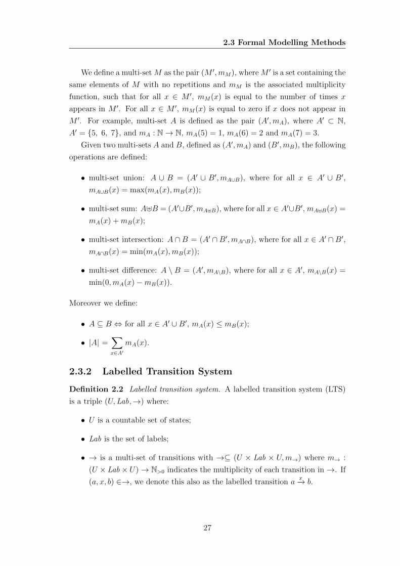
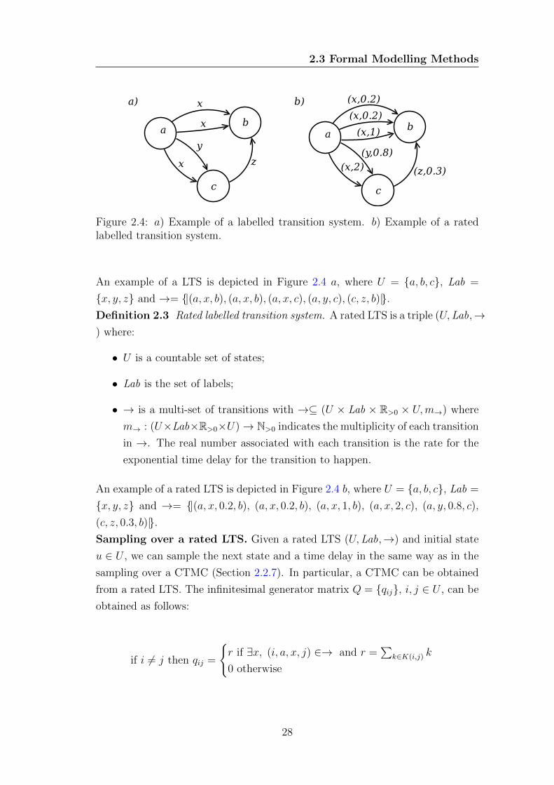
Figure 2.4: a) Example of a labelled transition system. b) Example of a ratedlabelled transition system.
An example of a LTS is depicted in Figure 2.4 a, where U = {a, b, c}, Lab =
{x, y, z} and →= {|(a, x, b), (a, x, b), (a, x, c), (a, y, c), (c, z, b)|}.Definition 2.3 Rated labelled transition system. A rated LTS is a triple (U,Lab,→) where:
• U is a countable set of states;
• Lab is the set of labels;
• → is a multi-set of transitions with →⊆ (U × Lab × R>0 × U,m→) where
m→ : (U×Lab×R>0×U)→ N>0 indicates the multiplicity of each transition
in →. The real number associated with each transition is the rate for the
exponential time delay for the transition to happen.
An example of a rated LTS is depicted in Figure 2.4 b, where U = {a, b, c}, Lab =
{x, y, z} and →= {|(a, x, 0.2, b), (a, x, 0.2, b), (a, x, 1, b), (a, x, 2, c), (a, y, 0.8, c),
(c, z, 0.3, b)|}.Sampling over a rated LTS. Given a rated LTS (U,Lab,→) and initial state
u ∈ U , we can sample the next state and a time delay in the same way as in the
sampling over a CTMC (Section 2.2.7). In particular, a CTMC can be obtained
from a rated LTS. The infinitesimal generator matrix Q = {qij}, i, j ∈ U , can be
obtained as follows:
if i 6= j then qij =
{r if ∃x, (i, a, x, j) ∈→ and r =
∑k∈K(i,j) k
0 otherwise
28
2.3 Formal Modelling Methods
qii = −∑
j 6=i qij
where K(i, j) = {|k | (i, a, k, j) ∈→ |}.
2.3.3 An Introduction to Process Algebra
Fundamental concepts. A process algebra is characterised by a syntax and by
one or more semantics. While the former defines how a process algebra model
is written, the latter defines how the behaviour of a model is determined from
its syntactic definition. The fundamental elements in a process algebra are au-
tonomous agents called processes. Each process is characterised by its behaviour,
expressed in terms of actions it can perform. For example, if a process P performs
a sequence of three a actions, we can denote it as:
P , a.a.a.nil
where “.” is the sequential operator and nil is defined as the deadlock process,
i.e. the process that cannot perform any action. A labelled transition is usually
employed to show that process can perform an action and become another process.
For example, P can perform action a and become process P ′, defined as P ′ ,
a.a.nil. This is denoted as:
Pa−→ P ′
Process P ′ is called a one-step derivative of P , while if a process can be obtained
after any number of transitions from P , this is called simply a derivative of P .
The set of derivatives of a processes and all the labelled transitions from such
derivatives form a derivation graph, which is an LTS where the set of states U is
the set of all derivatives and the set of labels Lab is the set of all actions.
It could be the case that process P can choose non deterministically between
multiple actions available. This is denoted using the choice operator “+”. For
example:
Q , a.nil + b.nil + c.d.nil
Here Q can produce the following three labelled transitions:
Qa−→ nil Q
b−→ nil Qc−→ d.nil
29
2.3 Formal Modelling Methods
Most importantly, processes can synchronise on actions. Synchronisation can be
binary between two actions with complementary names, in the style of calculus of
communicating systems (CCS) (Milner, 1989), or multi-way between any number
of actions sharing the same name, in the style of communicating sequential pro-
cesses (CSP) (Hoare, 1985) and later of performance evaluation process algebra
(PEPA) (Hillston, 1996). As we anticipated in the introduction to this thesis,
we follow the latter approach. Multi-way synchronisation is possible using the
cooperation operator BCL
. The set of actions L, or cooperation set, indicates
which actions are used for synchronisation. For example, given the processes:
R , a.nil + b.nil S , a.nil + b.nil + c.nil
and the overall model defined as R BC{a,c}
S, we have that only the following tran-
sitions are possible:
R BC{a,c}
Sa−→ nil BC
{a,c}nil R BC
{a,c}S
b−→ nil BC{a,c}
S R BC{a,c}
Sb−→ R BC
{a,c}nil
Because action a is in the cooperation set, R and S can synchronise on a, but
cannot perform a individually. On the contrary, b is not in the cooperation set,
so R and S cannot synchronise on b, though they can perform b individually.
Finally, c cannot be performed by S, because it is present in the cooperation set,
which would require that also R had the possibility of performing c.
Another key feature of process algebra is the possibility for actions to become
hidden. This is usually expressed by replacing the name of an action with the
hidden action type τ . This substitution may happen in an implicit way, as in CCS,
or in an explicit way, as in CSP. In CCS, as a result of a binary synchronisation,
the name of the two complementary actions that synchronise is replaced by τ .
As no other actions will synchronise, there is no need for the rest of the system
to know what specific action took place, information that is therefore considered
internal to the participants to the synchronisation. In contrast, in CSP there is
no way to know how many processes will synchronise, because of the multi-way
synchronisation. For this reason it is the responsibility of the modeller to place
hiding (\) operators appropriately in the system. For example, with R BC{a,c}
S \{b}we impose that if R BC
{a,c}S can perform action b, that action will be replaced with
τ upon application of \{b}. This results in the following labelled transitions:
(R BC{a,c}
S) \ {b} a−→ (nil BC{a,c}
nil) \ {b} (R BC{a,c}
S) \ {b} τ−→ (nil BC{a,c}
S) \ {b}(R BC
{a,c}S) \ {b} τ−→ (R BC
{a,c}nil) \ {b}
30
2.3 Formal Modelling Methods
Action Priorities. Action priorities have been introduced in the process algebra
theory to model interrupt mechanisms in computer systems (Baeten et al., 1986;
Cleaveland and Hennessy, 1990). In this extension, p:a indicates that action a is
performed with priority p, with p ∈ (N \ {0}). Actions with higher priority have
precedence and block actions with lower priority. Consider the following process:
Q , 1:a.nil + 2:b.nil + 3:c.1:d.nil
The only enabled labelled transition is Qc−→ 1:d.nil, because action c has the
highest priority if compared with the other available actions a and b. Moreover,
consider the following processes:
R , 1:a.nil + 2:b.nil S , 1:a.nil + 2:b.nil + 3:c.nil
In this case, the only enabled transitions are:
R BC{a,c}
Sb−→ nil BC
{a,c}S R BC
{a,c}S
b−→ R BC{a,c}
nil
Because although the action with highest priority is c, c is not available, i.e. it
cannot be performed by process R BC{a,c}
S. This is because c is in the cooperation
set of BC{a,c}
and is available in S, but not in R.
Relations. Finally, relations are usually defined between processes, to express
to which extent the behaviour of two processes can be considered the same. In
particular, fundamental to every process algebra theory are the notions of equiv-
alences, such as isomorphism or bisimulation (Milner, 1989), and whether such
equivalences are also congruences or not. In general, if an equivalence relation is
a congruence it ensures that the substitution of a process within a system with
an equivalent process will produce a system which is identical to the original one,
at least with respect to the behaviour preserved by the chosen equivalence.
2.3.4 Process Algebras for Biology
Modelling biological systems with existing formalisms, either algebras, calculi or
languages, requires an abstraction, i.e. a matching between biological entities
and the syntactic components of the chosen formalism.
In process algebra, this was first introduced with the “molecule-as-computation”
abstraction (Regev et al., 2001), using π-calculus (Milner, 1999) where each
31
2.3 Formal Modelling Methods
molecule in a system is represented by one or more concurrent processes, abstract-
ing the behaviour and/or interactions it might have. Two molecules can react
when their corresponding processes share a complementary channel, abstracting
complementary binding sites. An example is the following process definition of a
molecule M:
M , (νm)x!m.(m!a+m?a) + x?p.(p!a+ p?a)
where x!m represents the action of sending the name m into channel x and x?p
is the action of receiving from channel x a name that will replace p and all its oc-
currences in the local sequence of actions. Symbols ‘.’, ‘+’ and ‘|’ are respectively
the sequential operator, the choice operator and the parallel operator. Synchro-
nisation can happen only in a binary fashion, when a send and a receive action
that are divided by a parallel operator are executed together. Symbol νm is the
scope restriction of the name m, and it is often used to delimit the processes that
define a molecule or to restrict interactions, implementing compartmentalisation.
On the one hand, π-calculus is mathematically well understood and brings
with it many associated tools. On the other hand, it may be a too low-level
language. The language beta binders (Priami and Quaglia, 2005) tries to im-
prove this aspect by enriching the syntax inserting the processes that abstract
the behaviour of a biological entity in a box. Boxes are allowed to communicate
internally, as in π-calculus, and externally, through special channels, or interfaces.
A set of types is assigned to each channel that is used for external communica-
tions. Two boxes can then interact if they share at least one type, leading to
more flexibility and higher non-determinism. Finally, boxes can fuse or divide
using two types of function, join and split, that are essentially rewriting rules.
This is an example of the parallel instantiation of two beta binders bio-processes:
β(x : {a, b})[!xz.P1|Q1] ‖ β(y : {a, c})[?yu.P2|Q2]
where the boxes containing an extended version of π-calculus processes are de-
limited by the brackets [·] and the interfaces are declared within the β(·). In this
case x is an external channel with types a and b. The two boxes can interact via
channels x and y, because they share a common type a.
32
2.3 Formal Modelling Methods
The languages π-calculus and beta binders present similar drawbacks. They
are highly expressive languages that allow many ways to model the same system,
requiring experts to perform the modelling. Moreover, the level of detail that is
considered might be too high for the usual need of biologists. This is because
often not all the interactions are well understood and, considering quantitative
analysis, it is extremely difficult to obtain reliable stochastic rates for all the
events or a sufficient amount of measurements for all the states an entity can
assume.
A different approach is taken by PEPA (Hillston, 1996). The syntax of this
language is much simpler, without the notion of passing of information through
communication. An important characteristic is the synchronisation not only be-
tween two processes that present complementary channels, but between all pro-
cesses that share the same available action name, allowing the modelling of re-
actions that involve an arbitrary number of molecular species. Because of this,
the PEPA approach has the flexibility of abstracting more than one biological
interaction with a single action.
Although modelling each molecule as a process is possible, a population ap-
proach has been preferred in current PEPA applications. This means that a pro-
cess represents the number of molecules or the level of concentration of a species.
After an event is observed, these processes change to new processes expressing
different quantities. This approach is denoted “species-as-process” abstraction.
This is an example:
AH , (α1, r1).AL AL , (α2, r2).AH
BH , (α2, r2).BL BL , (α1, r1).BH
AH BC{α1,α2}BL
α1−→ AL BC{α1,α2}BH
Here two species A and B are modelled using processes that represent their
amount in the system, either high or low. α1 and α2 are the actions on which
the processes can synchronise, while r1 and r2 are the rates at which the actions
occur. The labelled transition shows what happens if α1 takes place from an
initial system AH BCα1,α2
BL.
Bio-PEPA (Ciocchetta and Hillston, 2009) is an extension of PEPA specifi-
cally designed to model biochemical interactions with a “species-as-process” ab-
33
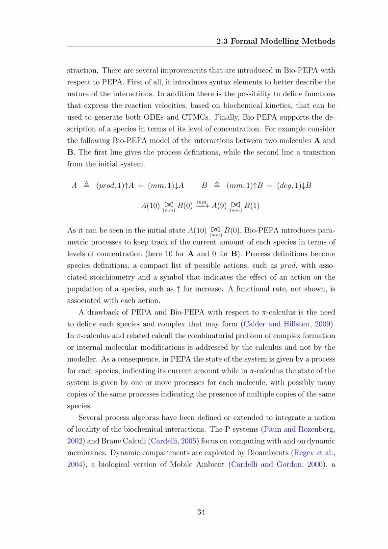
2.3 Formal Modelling Methods
straction. There are several improvements that are introduced in Bio-PEPA with
respect to PEPA. First of all, it introduces syntax elements to better describe the
nature of the interactions. In addition there is the possibility to define functions
that express the reaction velocities, based on biochemical kinetics, that can be
used to generate both ODEs and CTMCs. Finally, Bio-PEPA supports the de-
scription of a species in terms of its level of concentration. For example consider
the following Bio-PEPA model of the interactions between two molecules A and
B. The first line gives the process definitions, while the second line a transition
from the initial system.
A , (prod, 1)↑A + (mm, 1)↓A B , (mm, 1)↑B + (deg, 1)↓B
A(10) BC{mm}
B(0)mm−−→ A(9) BC
{mm}B(1)
As it can be seen in the initial state A(10) BC{mm}
B(0), Bio-PEPA introduces para-
metric processes to keep track of the current amount of each species in terms of
levels of concentration (here 10 for A and 0 for B). Process definitions become
species definitions, a compact list of possible actions, such as prod, with asso-
ciated stoichiometry and a symbol that indicates the effect of an action on the
population of a species, such as ↑ for increase. A functional rate, not shown, is
associated with each action.
A drawback of PEPA and Bio-PEPA with respect to π-calculus is the need
to define each species and complex that may form (Calder and Hillston, 2009).
In π-calculus and related calculi the combinatorial problem of complex formation
or internal molecular modifications is addressed by the calculus and not by the
modeller. As a consequence, in PEPA the state of the system is given by a process
for each species, indicating its current amount while in π-calculus the state of the
system is given by one or more processes for each molecule, with possibly many
copies of the same processes indicating the presence of multiple copies of the same
species.
Several process algebras have been defined or extended to integrate a notion
of locality of the biochemical interactions. The P-systems (Paun and Rozenberg,
2002) and Brane Calculi (Cardelli, 2005) focus on computing with and on dynamic
membranes. Dynamic compartments are exploited by Bioambients (Regev et al.,
2004), a biological version of Mobile Ambient (Cardelli and Gordon, 2000), a
34
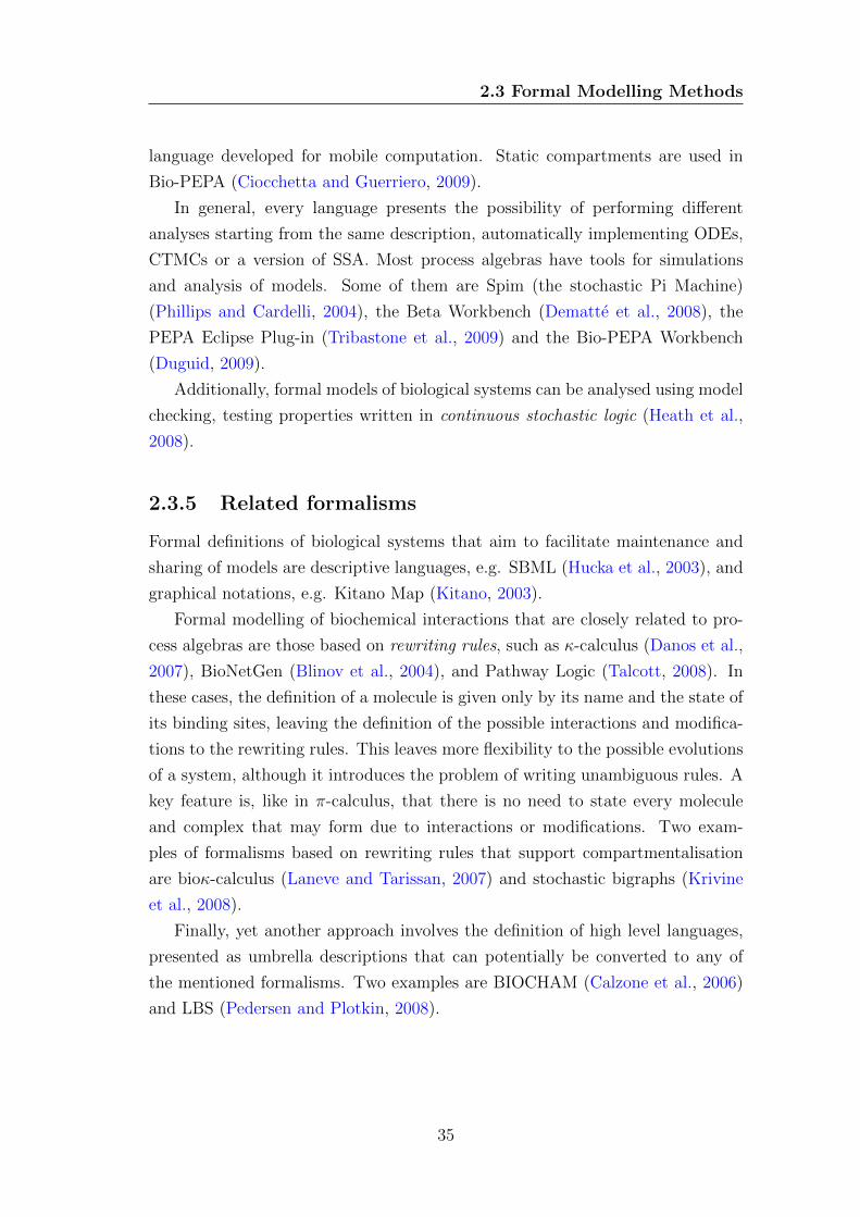
2.3 Formal Modelling Methods
language developed for mobile computation. Static compartments are used in
Bio-PEPA (Ciocchetta and Guerriero, 2009).
In general, every language presents the possibility of performing different
analyses starting from the same description, automatically implementing ODEs,
CTMCs or a version of SSA. Most process algebras have tools for simulations
and analysis of models. Some of them are Spim (the stochastic Pi Machine)
(Phillips and Cardelli, 2004), the Beta Workbench (Dematte et al., 2008), the
PEPA Eclipse Plug-in (Tribastone et al., 2009) and the Bio-PEPA Workbench
(Duguid, 2009).
Additionally, formal models of biological systems can be analysed using model
checking, testing properties written in continuous stochastic logic (Heath et al.,
2008).
2.3.5 Related formalisms
Formal definitions of biological systems that aim to facilitate maintenance and
sharing of models are descriptive languages, e.g. SBML (Hucka et al., 2003), and
graphical notations, e.g. Kitano Map (Kitano, 2003).
Formal modelling of biochemical interactions that are closely related to pro-
cess algebras are those based on rewriting rules, such as κ-calculus (Danos et al.,
2007), BioNetGen (Blinov et al., 2004), and Pathway Logic (Talcott, 2008). In
these cases, the definition of a molecule is given only by its name and the state of
its binding sites, leaving the definition of the possible interactions and modifica-
tions to the rewriting rules. This leaves more flexibility to the possible evolutions
of a system, although it introduces the problem of writing unambiguous rules. A
key feature is, like in π-calculus, that there is no need to state every molecule
and complex that may form due to interactions or modifications. Two exam-
ples of formalisms based on rewriting rules that support compartmentalisation
are bioκ-calculus (Laneve and Tarissan, 2007) and stochastic bigraphs (Krivine
et al., 2008).
Finally, yet another approach involves the definition of high level languages,
presented as umbrella descriptions that can potentially be converted to any of
the mentioned formalisms. Two examples are BIOCHAM (Calzone et al., 2006)
and LBS (Pedersen and Plotkin, 2008).
35
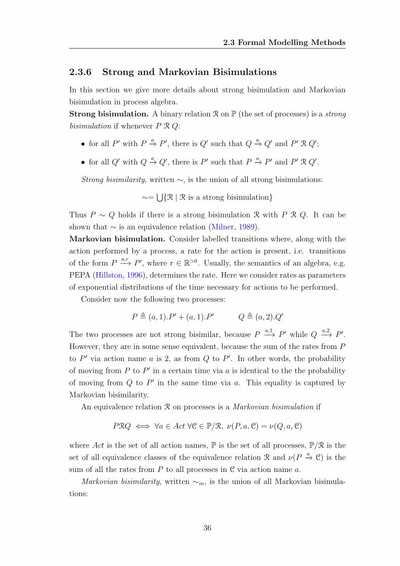
2.3 Formal Modelling Methods
2.3.6 Strong and Markovian Bisimulations
In this section we give more details about strong bisimulation and Markovian
bisimulation in process algebra.
Strong bisimulation. A binary relation R on P (the set of processes) is a strong
bisimulation if whenever P R Q:
• for all P ′ with Pa−→ P ′, there is Q′ such that Q
a−→ Q′ and P ′ R Q′;
• for all Q′ with Qa−→ Q′, there is P ′ such that P
a−→ P ′ and P ′ R Q′.
Strong bisimilarity, written ∼, is the union of all strong bisimulations:
∼=⋃{R | R is a strong bisimulation}
Thus P ∼ Q holds if there is a strong bisimulation R with P R Q. It can be
shown that ∼ is an equivalence relation (Milner, 1989).
Markovian bisimulation. Consider labelled transitions where, along with the
action performed by a process, a rate for the action is present, i.e. transitions
of the form Pa,r−→ P ′, where r ∈ R>0. Usually, the semantics of an algebra, e.g.
PEPA (Hillston, 1996), determines the rate. Here we consider rates as parameters
of exponential distributions of the time necessary for actions to be performed.
Consider now the following two processes:
P , (a, 1).P ′ + (a, 1).P ′ Q , (a, 2).Q′
The two processes are not strong bisimilar, because Pa,1−→ P ′ while Q
a,2−→ P ′.
However, they are in some sense equivalent, because the sum of the rates from P
to P ′ via action name a is 2, as from Q to P ′. In other words, the probability
of moving from P to P ′ in a certain time via a is identical to the the probability
of moving from Q to P ′ in the same time via a. This equality is captured by
Markovian bisimilarity.
An equivalence relation R on processes is a Markovian bisimulation if
PRQ ⇐⇒ ∀a ∈ Act ∀C ∈ P/R, ν(P, a,C) = ν(Q, a,C)
where Act is the set of all action names, P is the set of all processes, P/R is the
set of all equivalence classes of the equivalence relation R and ν(Pa−→ C) is the
sum of all the rates from P to all processes in C via action name a.
Markovian bisimilarity, written ∼m, is the union of all Markovian bisimula-
tions:
36
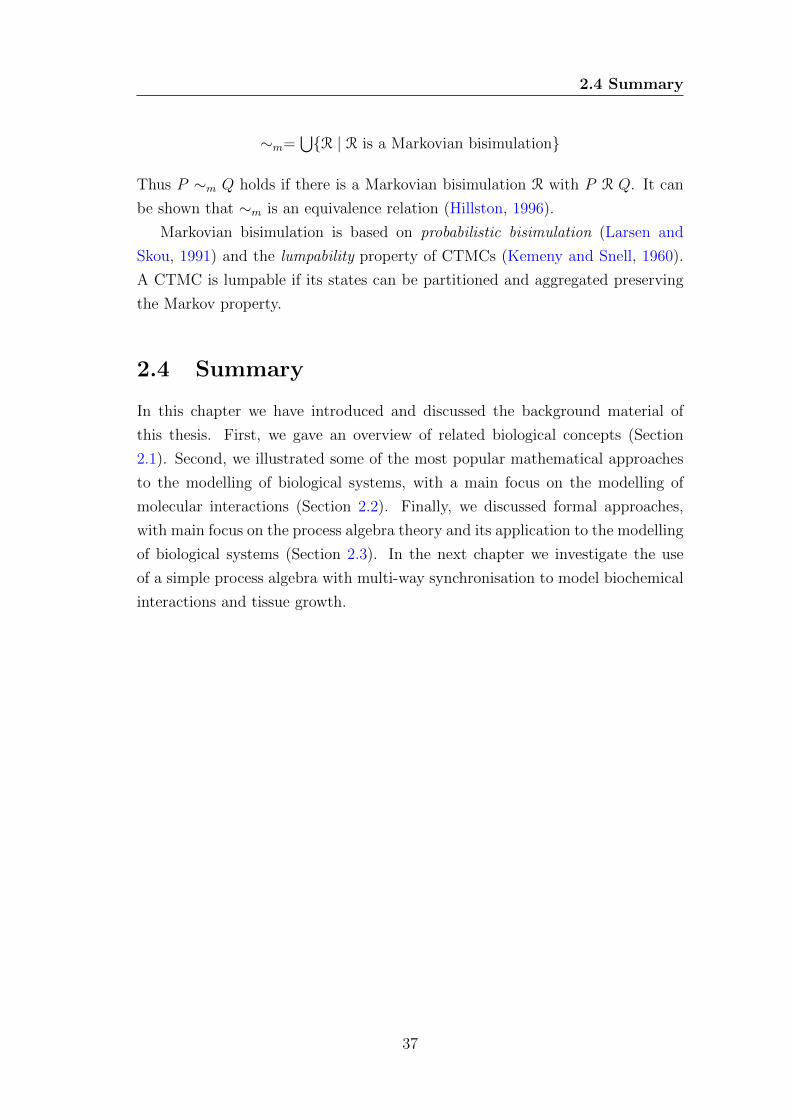
2.4 Summary
∼m=⋃{R | R is a Markovian bisimulation}
Thus P ∼m Q holds if there is a Markovian bisimulation R with P R Q. It can
be shown that ∼m is an equivalence relation (Hillston, 1996).
Markovian bisimulation is based on probabilistic bisimulation (Larsen and
Skou, 1991) and the lumpability property of CTMCs (Kemeny and Snell, 1960).
A CTMC is lumpable if its states can be partitioned and aggregated preserving
the Markov property.
2.4 Summary
In this chapter we have introduced and discussed the background material of
this thesis. First, we gave an overview of related biological concepts (Section
2.1). Second, we illustrated some of the most popular mathematical approaches
to the modelling of biological systems, with a main focus on the modelling of
molecular interactions (Section 2.2). Finally, we discussed formal approaches,
with main focus on the process algebra theory and its application to the modelling
of biological systems (Section 2.3). In the next chapter we investigate the use
of a simple process algebra with multi-way synchronisation to model biochemical
interactions and tissue growth.
37
Chapter 3
Single-Scale Modelling with
Process Algebra with Multi-way
Synchronisation
In this chapter we show how biological systems can be modelled with a process
algebra with multi-way synchronisation, focussing on a single scale. First, we dis-
cuss how to represent biological entities and events with processes and actions,
using a simple process algebra with multi-way synchronisation (Section 3.1). Sec-
ond, we augment the algebra with functional rates, obtaining a stochastic simple
process algebra (Section 3.2.1). With this augmented algebra, quantitative mod-
els can be constructed. Finally, we show how processes can be parametrised to
reduce the model definition (Section 3.3). We give example models of biochemical
reactions and tissue growth (Sections 3.1.1, 3.1.2, 3.2.5, 3.3.2).
3.1 Simple Process Algebra
A minimal syntax of a process algebra with multi-way synchronisation (SPA) is:
P ::= nil | a.P | P + P | P BCLP | A
where:
• P is a process, P ∈ P, with P the set of processes;
38
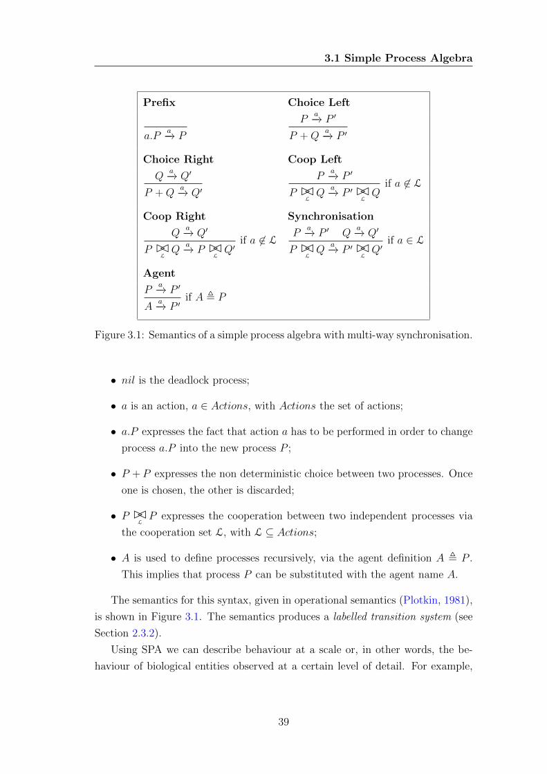
3.1 Simple Process Algebra
Prefix Choice Left
a.Pa−→ P
Pa−→ P ′
P +Qa−→ P ′
Choice Right Coop Left
Qa−→ Q′
P +Qa−→ Q′
Pa−→ P ′
P BCLQ
a−→ P ′ BCLQ
if a 6∈ L
Coop Right Synchronisation
Qa−→ Q′
P BCLQ
a−→ P BCLQ′
if a 6∈ LP
a−→ P ′ Qa−→ Q′
P BCLQ
a−→ P ′ BCLQ′
if a ∈ L
Agent
Pa−→ P ′
Aa−→ P ′
if A , P
Figure 3.1: Semantics of a simple process algebra with multi-way synchronisation.
• nil is the deadlock process;
• a is an action, a ∈ Actions, with Actions the set of actions;
• a.P expresses the fact that action a has to be performed in order to change
process a.P into the new process P ;
• P + P expresses the non deterministic choice between two processes. Once
one is chosen, the other is discarded;
• P BCLP expresses the cooperation between two independent processes via
the cooperation set L, with L ⊆ Actions;
• A is used to define processes recursively, via the agent definition A , P .
This implies that process P can be substituted with the agent name A.
The semantics for this syntax, given in operational semantics (Plotkin, 1981),
is shown in Figure 3.1. The semantics produces a labelled transition system (see
Section 2.3.2).
Using SPA we can describe behaviour at a scale or, in other words, the be-
haviour of biological entities observed at a certain level of detail. For example,
39
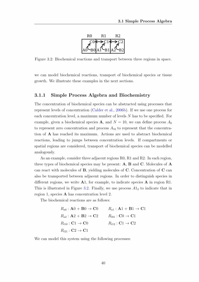
3.1 Simple Process Algebra
Figure 3.2: Biochemical reactions and transport between three regions in space.
we can model biochemical reactions, transport of biochemical species or tissue
growth. We illustrate these examples in the next sections.
3.1.1 Simple Process Algebra and Biochemistry
The concentration of biochemical species can be abstracted using processes that
represent levels of concentration (Calder et al., 2006b). If we use one process for
each concentration level, a maximum number of levels N has to be specified. For
example, given a biochemical species A, and N = 10, we can define process A0
to represent zero concentration and process A10 to represent that the concentra-
tion of A has reached its maximum. Actions are used to abstract biochemical
reactions, leading to jumps between concentration levels. If compartments or
spatial regions are considered, transport of biochemical species can be modelled
analogously.
As an example, consider three adjacent regions R0, R1 and R2. In each region,
three types of biochemical species may be present: A, B and C. Molecules of A
can react with molecules of B, yielding molecules of C. Concentration of C can
also be transported between adjacent regions. In order to distinguish species in
different regions, we write A1, for example, to indicate species A in region R1.
This is illustrated in Figure 3.2. Finally, we use process A12 to indicate that in
region 1, species A has concentration level 2.
The biochemical reactions are as follows:
Ra0 : A0 + B0 → C0 Ra1 : A1 + B1 → C1
Ra2 : A2 + B2 → C2 Rt01 : C0 → C1
Rt10 : C1 → C0 Rt12 : C1 → C2
Rt21 : C2 → C1
We can model this system using the following processes:
40
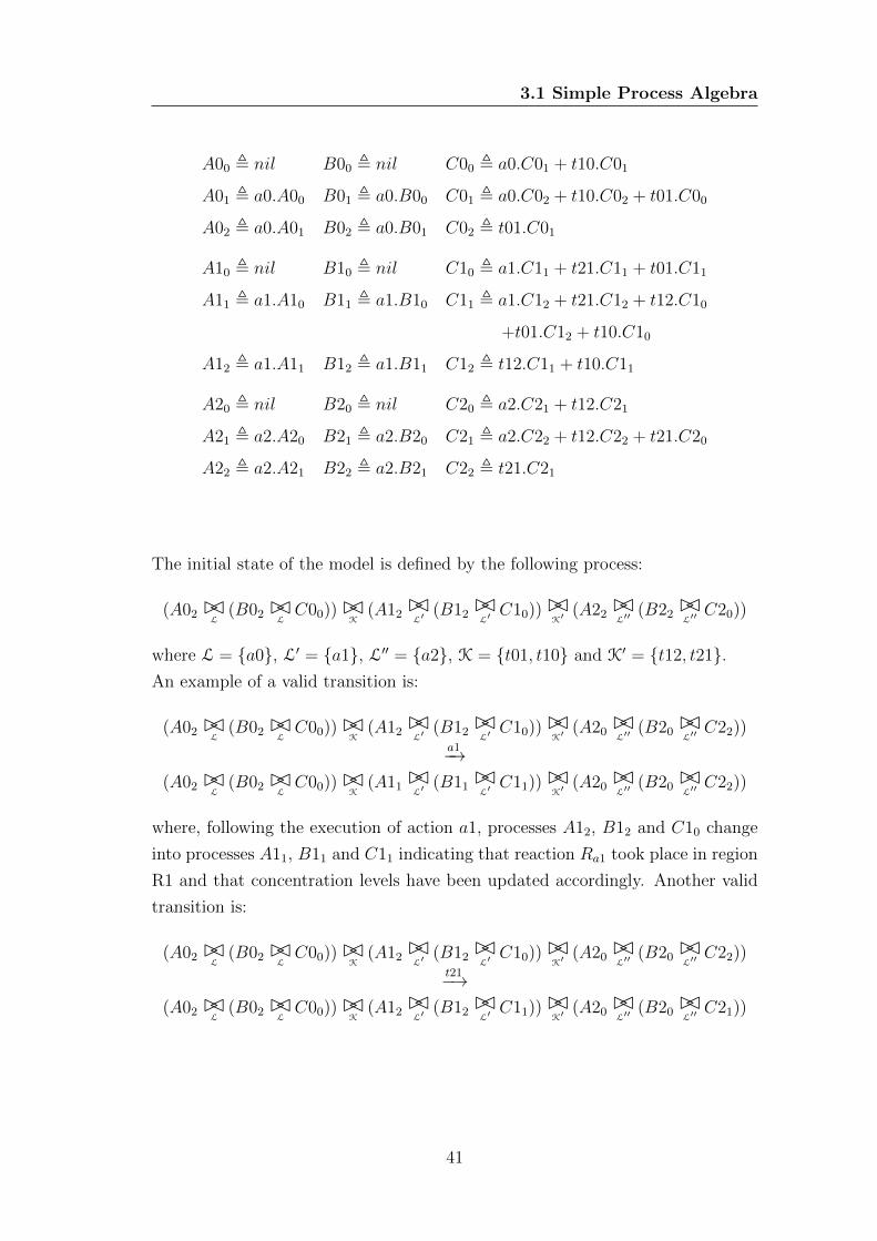
3.1 Simple Process Algebra
A00 , nil B00 , nil C00 , a0.C01 + t10.C01
A01 , a0.A00 B01 , a0.B00 C01 , a0.C02 + t10.C02 + t01.C00
A02 , a0.A01 B02 , a0.B01 C02 , t01.C01
A10 , nil B10 , nil C10 , a1.C11 + t21.C11 + t01.C11
A11 , a1.A10 B11 , a1.B10 C11 , a1.C12 + t21.C12 + t12.C10
+t01.C12 + t10.C10
A12 , a1.A11 B12 , a1.B11 C12 , t12.C11 + t10.C11
A20 , nil B20 , nil C20 , a2.C21 + t12.C21
A21 , a2.A20 B21 , a2.B20 C21 , a2.C22 + t12.C22 + t21.C20
A22 , a2.A21 B22 , a2.B21 C22 , t21.C21
The initial state of the model is defined by the following process:
(A02 BCL
(B02 BCLC00))BC
K(A12BCL′
(B12BCL′C10))BC
K′(A22BCL′′
(B22BCL′′C20))
where L = {a0}, L′ = {a1}, L′′ = {a2}, K = {t01, t10} and K′ = {t12, t21}.An example of a valid transition is:
(A02 BCL
(B02 BCLC00))BC
K(A12BCL′
(B12BCL′C10))BC
K′(A20BCL′′
(B20BCL′′C22))
a1−→(A02 BC
L(B02 BC
LC00))BC
K(A11BCL′
(B11BCL′C11))BC
K′(A20BCL′′
(B20BCL′′C22))
where, following the execution of action a1, processes A12, B12 and C10 change
into processes A11, B11 and C11 indicating that reaction Ra1 took place in region
R1 and that concentration levels have been updated accordingly. Another valid
transition is:
(A02 BCL
(B02 BCLC00))BC
K(A12BCL′
(B12BCL′C10))BC
K′(A20BCL′′
(B20BCL′′C22))
t21−→(A02 BC
L(B02 BC
LC00))BC
K(A12BCL′
(B12BCL′C11))BC
K′(A20BCL′′
(B20BCL′′C21))
41
3.1 Simple Process Algebra
where, following the execution of action t21, processes C22 and C10 change into
processes C21 and C11, indicating that transport of concentration of C took place
from region R2 to region R1.
A disadvantage of SPA is that every region requires the definition of its own
processes, yielding long and repetitive process algebra descriptions. This will be
improved with the introduction of parametric processes and actions (Section 3.3).
To give an idea of the different style of modelling of the π-calculus with respect
to SPA, we reproduce here an example of a biochemical reaction Ra : A + B →C from (Regev, 2002).
In π-calculus all molecules present in the system are modelled. In the case of
reaction Ra we need definitions of processes representing molecules A and B in
both bound and unbound states. Definitions are as follows:
A , (νx)(bind !x.BoundA(x))
BoundA(x) , x!a.A
B , bind?y.BoundB(y)
BoundB(y) , y?b.B
where (νx)(P ) means that the channel name x is private to process P , bind !x is
an send action, expressing the sending of action name x through channel bind ,
and bind?y is a receive action, expressing the receiving of name y through channel
bind . Processes BoundA(x) and BoundB(y) are parametric processes.
The initial state of the system is given by the cooperation between A and B
processes, for example:
A|B|A|B|A|B
where there are three A processes representing three A molecules and three B
processes representing three B molecules. At the execution of action bind !x by
a process A, private channel x is shared with a process B, by synchronisation
with action bind?y. Selection of exactly one process A and one process B for the
synchronisation is possible because synchronisation in π-calculus is binary and
can happen only between a send and a receive sharing the same channel name
(bind). This results in the new state:
(νx)(BoundA(x)|BoundB(x))|A|B|A|B
42
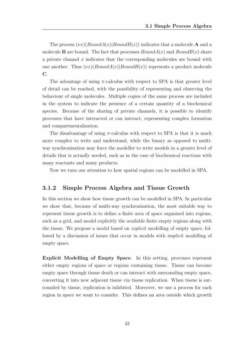
3.1 Simple Process Algebra
The process (νx)(BoundA(x)|BoundB(x)) indicates that a molecule A and a
molecule B are bound. The fact that processes BoundA(x) and BoundB(x) share
a private channel x indicates that the corresponding molecules are bound with
one another. Thus (νx)(BoundA(x)|BoundB(x)) represents a product molecule
C.
The advantage of using π-calculus with respect to SPA is that greater level
of detail can be reached, with the possibility of representing and observing the
behaviour of single molecules. Multiple copies of the same process are included
in the system to indicate the presence of a certain quantity of a biochemical
species. Because of the sharing of private channels, it is possible to identify
processes that have interacted or can interact, representing complex formation
and compartmentalisation.
The disadvantage of using π-calculus with respect to SPA is that it is much
more complex to write and understand, while the binary as opposed to multi-
way synchronisation may force the modeller to write models in a greater level of
details that is actually needed, such as in the case of biochemical reactions with
many reactants and many products.
Now we turn our attention to how spatial regions can be modelled in SPA.
3.1.2 Simple Process Algebra and Tissue Growth
In this section we show how tissue growth can be modelled in SPA. In particular
we show that, because of multi-way synchronisation, the most suitable way to
represent tissue growth is to define a finite area of space organised into regions,
such as a grid, and model explicitly the available finite empty regions along with
the tissue. We propose a model based on explicit modelling of empty space, fol-
lowed by a discussion of issues that occur in models with implicit modelling of
empty space.
Explicit Modelling of Empty Space. In this setting, processes represent
either empty regions of space or regions containing tissue. Tissue can become
empty space through tissue death or can interact with surrounding empty space,
converting it into new adjacent tissue via tissue replication. When tissue is sur-
rounded by tissue, replication is inhibited. Moreover, we use a process for each
region in space we want to consider. This defines an area outside which growth
43
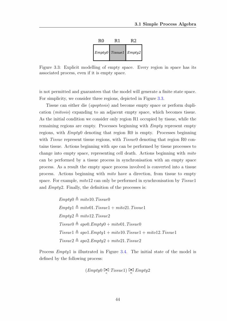
3.1 Simple Process Algebra
Figure 3.3: Explicit modelling of empty space. Every region in space has itsassociated process, even if it is empty space.
is not permitted and guarantees that the model will generate a finite state space.
For simplicity, we consider three regions, depicted in Figure 3.3.
Tissue can either die (apoptosis) and become empty space or perform dupli-
cation (mitosis) expanding to an adjacent empty space, which becomes tissue.
As the initial condition we consider only region R1 occupied by tissue, while the
remaining regions are empty. Processes beginning with Empty represent empty
regions, with Empty0 denoting that region R0 is empty. Processes beginning
with Tissue represent tissue regions, with Tissue0 denoting that region R0 con-
tains tissue. Actions beginning with apo can be performed by tissue processes to
change into empty space, representing cell death. Actions beginning with mito
can be performed by a tissue process in synchronisation with an empty space
process. As a result the empty space process involved is converted into a tissue
process. Actions beginning with mito have a direction, from tissue to empty
space. For example, mito12 can only be performed in synchronisation by Tissue1
and Empty2. Finally, the definition of the processes is:
Empty0 , mito10.Tissue0
Empty1 , mito01.Tissue1 + mito21.Tissue1
Empty2 , mito12.Tissue2
Tissue0 , apo0.Empty0 + mito01.Tissue0
Tissue1 , apo1.Empty1 + mito10.Tissue1 + mito12.Tissue1
Tissue2 , apo2.Empty2 + mito21.Tissue2
Process Empty1 is illustrated in Figure 3.4. The initial state of the model is
defined by the following process:
(Empty0BCL
Tissue1)BCK
Empty2
44
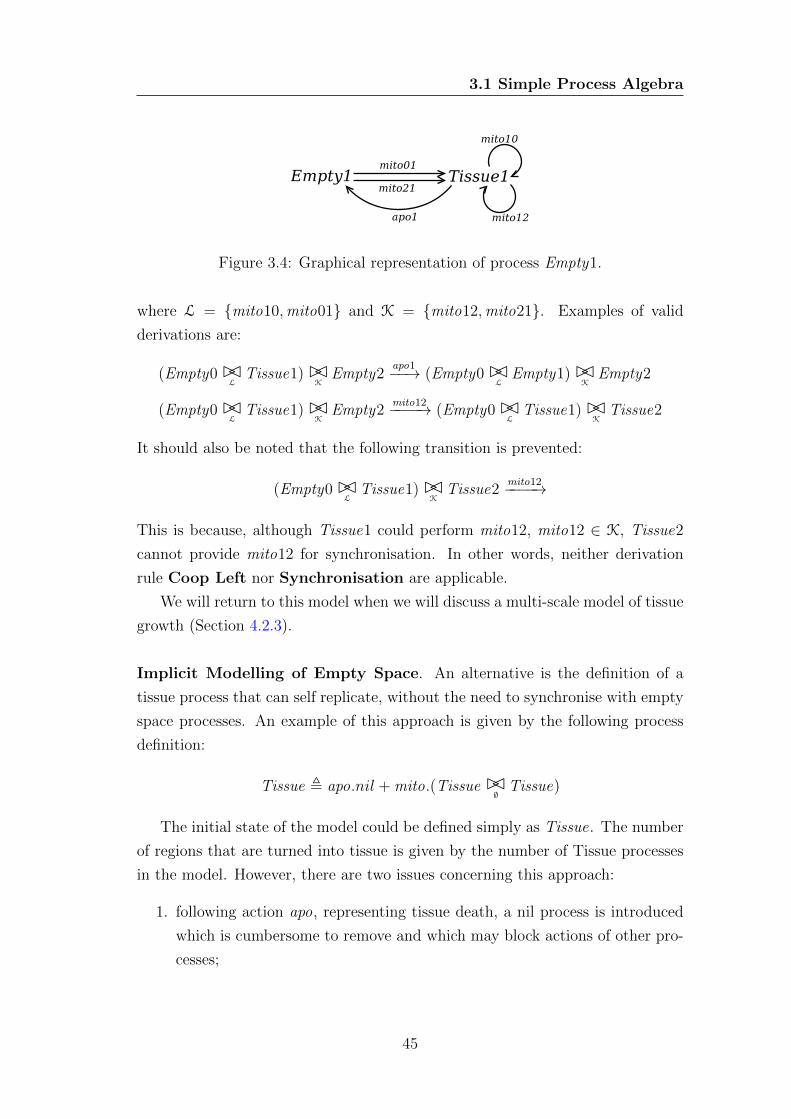
3.1 Simple Process Algebra
Figure 3.4: Graphical representation of process Empty1.
where L = {mito10,mito01} and K = {mito12,mito21}. Examples of valid
derivations are:
(Empty0BCL
Tissue1)BCK
Empty2apo1−−→ (Empty0BC
LEmpty1)BC
KEmpty2
(Empty0BCL
Tissue1)BCK
Empty2mito12−−−−→ (Empty0BC
LTissue1)BC
KTissue2
It should also be noted that the following transition is prevented:
(Empty0BCL
Tissue1)BCK
Tissue2mito12−−−−→
This is because, although Tissue1 could perform mito12, mito12 ∈ K, Tissue2
cannot provide mito12 for synchronisation. In other words, neither derivation
rule Coop Left nor Synchronisation are applicable.
We will return to this model when we will discuss a multi-scale model of tissue
growth (Section 4.2.3).
Implicit Modelling of Empty Space. An alternative is the definition of a
tissue process that can self replicate, without the need to synchronise with empty
space processes. An example of this approach is given by the following process
definition:
Tissue , apo.nil + mito.(Tissue BC∅
Tissue)
The initial state of the model could be defined simply as Tissue. The number
of regions that are turned into tissue is given by the number of Tissue processes
in the model. However, there are two issues concerning this approach:
1. following action apo, representing tissue death, a nil process is introduced
which is cumbersome to remove and which may block actions of other pro-
cesses;
45
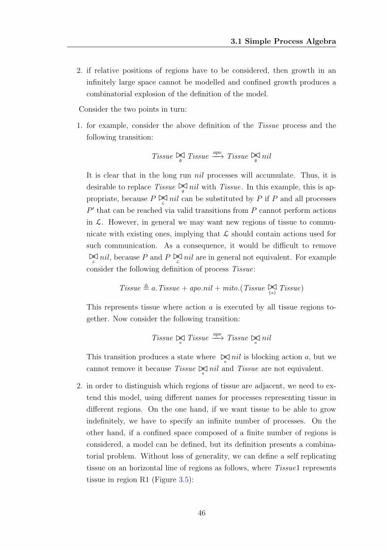
3.1 Simple Process Algebra
2. if relative positions of regions have to be considered, then growth in an
infinitely large space cannot be modelled and confined growth produces a
combinatorial explosion of the definition of the model.
Consider the two points in turn:
1. for example, consider the above definition of the Tissue process and the
following transition:
Tissue BC∅
Tissueapo−−→ Tissue BC
∅nil
It is clear that in the long run nil processes will accumulate. Thus, it is
desirable to replace Tissue BC∅nil with Tissue. In this example, this is ap-
propriate, because P BCLnil can be substituted by P if P and all processes
P ′ that can be reached via valid transitions from P cannot perform actions
in L. However, in general we may want new regions of tissue to commu-
nicate with existing ones, implying that L should contain actions used for
such communication. As a consequence, it would be difficult to remove
BCLnil, because P and P BC
Lnil are in general not equivalent. For example
consider the following definition of process Tissue:
Tissue , a.Tissue + apo.nil + mito.(Tissue BC{a}
Tissue)
This represents tissue where action a is executed by all tissue regions to-
gether. Now consider the following transition:
Tissue BCa
Tissueapo−−→ Tissue BC
anil
This transition produces a state where BCanil is blocking action a, but we
cannot remove it because Tissue BCanil and Tissue are not equivalent.
2. in order to distinguish which regions of tissue are adjacent, we need to ex-
tend this model, using different names for processes representing tissue in
different regions. On the one hand, if we want tissue to be able to grow
indefinitely, we have to specify an infinite number of processes. On the
other hand, if a confined space composed of a finite number of regions is
considered, a model can be defined, but its definition presents a combina-
torial problem. Without loss of generality, we can define a self replicating
tissue on an horizontal line of regions as follows, where Tissue1 represents
tissue in region R1 (Figure 3.5):
46
3.1 Simple Process Algebra
Figure 3.5: Implicit modelling of empty space on a line. Each region has a positionidentified by a natural number.
Tissue1 , apo1.nil + mito12.(Tissue1BC∅
Tissue2)
+mito10.(Tissue1BC∅
Tissue0))
The initial state of the model is given by the process Tissue1 alone. It is
clear that this definition is not appropriate, because it may lead to multiple
copies of process Tissue2. For example:
Tissue1mito12−−−−→ Tissue1BC
∅Tissue2
mito12−−−−→(Tissue1BC
∅Tissue2)BC
∅Tissue2
In order to overcome this problem, the definition of Tissue1 needs to encode
whether adjacent tissue is present or not. For example, if Tissue1 replicates
adding process Tissue2, Tissue1 has to be updated to avoid the addition
of another Tissue2 process. But this is not enough. If Tissue3 is present in
the model, it should be updated as well because it is adjacent to Tissue2.
Moreover, a similar neighbour update has to be performed when action
apo1 is performed.
Unfortunately, there is no trivial solution to this problem. We illustrate
why with an example. Assume we can define a Tissue1 (and analogous
definitions for Tissue2, Tissue3...) process as follows:
47
3.1 Simple Process Algebra
Tissue1 , apo1.nil + mito12.(Tissue1′ BCL
Tissue2)
+mito10.(Tissue1′′ BCK
Tissue0 + mito-10.Tissue1′′
+mito32.Tissue1′)
Tissue1′ , apo1.nil + apo2.Tissue1
+mito10.(Tissue1′′′ BCK
Tissue0) + mito-10.Tissue1′′′
Tissue1′′ , apo1.nil + apo0.Tissue1
+mito12.(Tissue1′′′ BCL
Tissue2) + mito32.Tissue1′′′
Tissue1′′′ , apo1.nil + apo2.Tissue1′′ + apo0.Tissue1′
The four Tissue1 processes represent different action capabilities of a re-
gion depending on the surrounding regions. Tissue1 expresses the actions
available when regions are empty on the left and on the right, Tissue1′
when tissue is present only on the right, Tissue1′′ when tissue is present
only on the left and Tissue1′′′ when tissue is surrounding the current region.
However, this solution is not correct. The reason is that since, for example,
Tissue1 is responsible for the addition of Tissue2, it should also be able to
determine which version of Tissue2 has to be introduced, choosing between
the four stated above and depending on whether Tissue3 is present or not.
In fact, because of this mechanism, if a model were composed of Tissue1
and Tissue100, the behaviour of Tissue1 would depend on the fact that
Tissue100 is present in the model. This implies a combinatorial explosion
of process definitions.
Another problem is the choice of cooperation sets L and K. For example,
apo(i) should be placed in both L and K, in order to communicate to
adjacent tissue that region i is empty again. However, once a Tissue process
becomes nil, there is no trivial way to remove it, blocking all the other
parametric actions in the two cooperation sets.
We can conclude that, because of the problems discussed in this section, in
the context of modelling tissue growth with multi-way synchronisation, the ex-
plicit modelling approach of empty space is preferable to the implicit modelling
approach of empty space.
48
3.2 Stochastic Semantics for Simple Process Algebra
3.2 Stochastic Semantics for Simple Process Al-
gebra
In this section we define a stochastic semantics based on functional rates for SPA.
The motivation for functional rates comes from the fact that rates of biological
events often depend on the current state of the system itself. More precisely, only
a part of a biological system contributes to the determination of the rate of an
event. In terms of process algebra, this means that an action is associated with
a set of processes and these processes are associated with variables and values
that are used to evaluate functional rates. An example is the evaluation of a
rate for a biochemical event. Processes represent the concentration of species
(the variables) and the current concentration level (the values). Functional rates
based on kinetic laws are associated with actions. When processes synchronise
via a specific action, the corresponding functional rate is evaluated according to
the information associated to the processes.
In order to obtain a stochastic semantics for SPA, with the characteristics
outlined above, we define:
• a new syntax for SPA, which should guarantee that at any time variables
and values can be associated with processes (Section 3.2.1);
• a new semantics that determines which actions are valid along with collect-
ing variables and values from the processes that participate in the actions.
In particular we use functions Var : Pm → Names and Val : Pm → R, with
Names the set of parameter names. Variables and values are stored into
an environment Γ. We define Γ as a partial function, with Γ : Names→ R.
We assume that Γ can be represented as a set of pairs of the form (n,Γ(n)) ∈Names×R. Moreover, we assume that Γ can be extended using set union.
The union Γ1 ∪ Γ2 is well defined only if for all a, b ∈ Names, if (a, x) ∈ Γ1
and (b, y) ∈ Γ2 then a 6= b. The semantics yields labelled transitions with
pairs (a,Γ) as labels, where a is an action and Γ an environment (Section
3.2.1);
• a syntax for functional rates (Section 3.2.2);
49
3.2 Stochastic Semantics for Simple Process Algebra
• a semantics for functional rates, that, given an environment determines
valid evaluations of a functional rate to an actual rate, i.e. a real number
(Section 3.2.2);
• a mechanism to decide when a functional rate can or cannot be evaluated for
a specified pair (a,Γ). This evaluation is performed on a derivation graph
generated by the semantics of the algebra and produces a rated derivation
graph, where rated labels have the form (a, r), with r ∈ R>0, while labels
that cannot be rated are unchanged (Section 3.2.4).
We illustrate some of the concepts just discussed with an example. Consider
the following biochemical reaction Ra between biochemical species A, B and C
and corresponding velocity va:
Ra :A+B→vaC, va = ka[A][B]
The velocity va expresses the amount of concentration of A and B that is con-
sumed per time unit. The symbol [·] means concentration, e.g. [A] is the con-
centration of species A, while ka is a constant. To represent the interactions of
Ra, we use the following processes:
A0 , nil B0 , nil C0 , a.C1
A1 , a.A0 B1 , a.B0 C1 , a.C2
A2 , a.A1 B2 , a.B1 C2 , nil
We use the processes as levels of concentration abstraction, in analogy with
Section 3.2. The three processes for each species represent a different concentra-
tion level, from 0 to 2. The maximum concentration is fixed to M , while N is the
maximum number of levels, here 2. The concentration represented by one level
is given by h, with h = M/N .
As explained above, we associate a variable name and a value to each of the
processes. To do so, we use functions Var(·) and Val(·). In particular we need to
provide the following information:
50
3.2 Stochastic Semantics for Simple Process Algebra
Var(A0) = levelA Var(B0) = levelB Var(C0) = levelC
Val(A0) = 0 Val(B0) = 0 Val(C0) = 0
Var(A1) = levelA Var(B1) = levelB Var(C1) = levelC
Val(A1) = 1 Val(B1) = 1 Val(C1) = 1
Var(A2) = levelA Var(B2) = levelB Var(C2) = levelC
Val(A2) = 2 Val(B2) = 2 Val(C2) = 2
The velocity va is used to produce the functional rate associated with action
a in analogy with that for CTMC with levels (Section 2.2.8):
fa = (ka · levelA · h · levelB · h)/h
This means that in order to evaluate fa we need to provide an additional environ-
ment containing values for constants h and ka. This could be Γ = {(h, 1), (ka, 1)}.Now assume that the initial state of the model is given by:
A2 BCa
(B2 BCaC0)
Intuitively, an appropriate stochastic semantics should permit the following
transition:
A2 BCa
(B2 BCaC0)
(a,ra)−−−→ A1 BCa
(B1 BCaC1)
with ra = 4, resulting from the evaluation of fa.
We propose that the aim of a stochastic semantics should be to determine
if an action a is possible and, at the same time, collect information about the
variables and values associated with the processes that synchronise on a. For
example, a valid transition is:
A2 BCa
(B2 BCaC0)
(a,Γ′)−−−→ A1 BCa
(B1 BCaC1)
with Γ′ = {(levelA, 2), (levelB, 2), (levelC, 0)}. We call the pair (a,Γ′) an activ-
ity. We can rate activity (a,Γ′) using Γ′, fa and the additional constant environ-
ment Γ containing values of variables h and ka. The result of the rating of (a,Γ′)
is the rated activity (a, ra).
51
3.2 Stochastic Semantics for Simple Process Algebra
3.2.1 Stochastic Simple Process Algebra
In order to define a suitable stochastic semantics for SPA, we first modify the
syntax. In particular, we want to make sure that variables and values can always
be associated with processes in a model. In order to do so, we associate variables
and values only with agents and restrict the model definition to cooperations of
agents. This means that agents now play a central role in the algebra. Thus,
we divide the syntax into definition processes (D) and model processes (M) as
follows:
D ::= nil | a.A | D +D
M ::= A |M BCLM
where:
• D is a definition process, D ∈ Pd, while M is a model process, M ∈ Pm.
Definition and model processes are disjoint and are both processes, i.e.
Pd ∪ Pm = P and Pd ∩ Pm = ∅;
• agent A is defined as A , D, that is we use definition processes to define
the behaviour of agents, restricting agent definitions to choices of actions;
• a model is defined by a model process M , which in turn is either an agent
A or a cooperation between model processes M BCLM ;
• action execution a.A is always followed by an agent A. This ensures that
at any time the state of a model will consist of a cooperation of agents;
• each agent A is associated with a variable and a value, that is functions
Var(A) ∈ Names, with Names the set of parameter names, and Val(A) ∈R must be defined for all agents A. This, along with the above definitions,
ensures that variables and values can always be associated with processes
in a model.
The stochastic semantics for this new syntax is shown in Figure 3.6. With
this semantics, information of variables and values is collected in the set Γ. In
the derivation rule Synchronisation, union of environments Γ1 and Γ2 is valid
only if for all a, b ∈ Names, if (a, x) ∈ Γ1 and (b, y) ∈ Γ2 then a 6= b. The
52
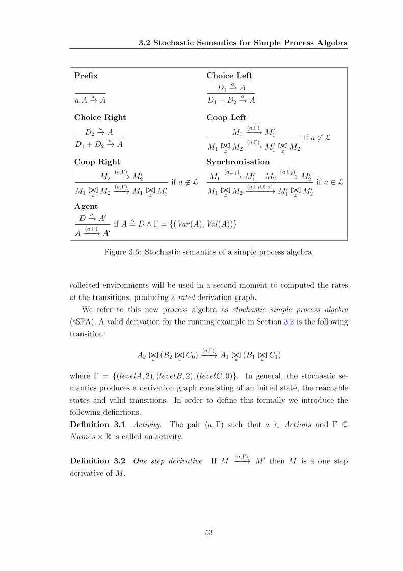
3.2 Stochastic Semantics for Simple Process Algebra
Prefix Choice Left
a.Aa−→ A
D1a−→ A
D1 +D2a−→ A
Choice Right Coop Left
D2a−→ A
D1 +D2a−→ A
M1(a,Γ)−−−→M ′
1
M1 BCLM2
(a,Γ)−−−→M ′1BCLM2
if a 6∈ L
Coop Right Synchronisation
M2(a,Γ)−−−→M ′
2
M1 BCLM2
(a,Γ)−−−→M1 BCLM ′
2
if a 6∈ LM1
(a,Γ1)−−−→M ′1 M2
(a,Γ2)−−−→M ′2
M1 BCLM2
(a,Γ1∪Γ2)−−−−−→M ′1BCLM ′
2
if a ∈ L
Agent
Da−→ A′
A(a,Γ)−−−→ A′
if A , D ∧ Γ = {(Var(A),Val(A))}
Figure 3.6: Stochastic semantics of a simple process algebra.
collected environments will be used in a second moment to computed the rates
of the transitions, producing a rated derivation graph.
We refer to this new process algebra as stochastic simple process algebra
(sSPA). A valid derivation for the running example in Section 3.2 is the following
transition:
A2 BCa
(B2 BCaC0)
(a,Γ)−−−→ A1 BCa
(B1 BCaC1)
where Γ = {(levelA, 2), (levelB, 2), (levelC, 0)}. In general, the stochastic se-
mantics produces a derivation graph consisting of an initial state, the reachable
states and valid transitions. In order to define this formally we introduce the
following definitions.
Definition 3.1 Activity. The pair (a,Γ) such that a ∈ Actions and Γ ⊆Names× R is called an activity.
Definition 3.2 One step derivative. If M(a,Γ)−−−→ M ′ then M is a one step
derivative of M .
53
3.2 Stochastic Semantics for Simple Process Algebra
Definition 3.3 Derivative. If Mi(a,Γ)−−−→ . . .
(a′,Γ′)−−−→ Mj then Mj is a derivative of
Mi.
Definition 3.4 Derivative Set. The derivative set of a model process M ∈ Pmis denoted by ds(M) and is defined as the smallest set of model processes such
that:
• M ∈ ds(M);
• if Mi ∈ ds(M) and Mi(a,Γ)−−−→Mj then Mj ∈ ds(M).
Definition 3.5 Current actions for definition processes. The set of actions that
D ∈ Pd can perform is denoted by Actions(D) and is defined as:
• Actions(nil) = {||};
• Actions(a.A) = {|a|};
• Actions(D1 +D2) = Actions(D1) ] Actions(D2).
with {||} delimiting a multi-set and ] the sum of multi-sets.
Definition 3.6 Current activities for model Processes. The set of activities that
M ∈ Pm can perform is denoted by Activities(M) and is defined as:
• Activities(A) = {|(a,Γ) | a ∈ Actions(D)∧A , D∧Γ = {(Var(A),Val(A))}|};
• Activities(M1 BCLM2) =
{|(a,Γ) | (a,Γ) ∈ Activities(M1) ∧ a 6∈ L|}] {|(a,Γ) | (a,Γ) ∈ Activities(M2) ∧ a 6∈ L|}]{|(a,Γ1∪Γ2) | (a,Γ1) ∈ Activities(M1)∧(a,Γ2) ∈ Activities(M2)∧a ∈ L|}.
Definition 3.7 Activity set. The set of all activities that a model process M ∈Pm or one of its derivatives can perform is given by:
−−−−−−→Activities(M) =
⊎Mi∈ds(M)
Activities(Mi)
54
3.2 Stochastic Semantics for Simple Process Algebra
Definition 3.8 Derivation graph. Given a model component M ∈ Pm, the
derivation graph D(M) is the labelled directed graph with:
• set of nodes ds(M);
• multi-set of transition labels−−−−−−→Activities(M);
• multi-set of labelled transitions→⊆ ds(M)×−−−−−−→Activities(M)×ds(M). Given
M ′ ∈ ds(M), (M ′, a,Γ,M ′′) ∈→ iff M ′ (a,Γ)−−−→M ′′.
The derivation graph of the running example of Section 3.2, D(A2 BCa
(B2 BCaC0))
is:
A2 BCa
(B2 BCaC0)
(a,Γ)−−−→ A1 BCa
(B1 BCaC1)
(a,Γ′)−−−→ A0 BCa
(B0 BCaC2)
with Γ = {(levelA, 2), (levelB, 2), (levelC, 0)} and Γ′ = {(levelA, 1), (levelB, 1),
(levelC, 1)}.Before we can introduce the formal definition of a rated derivation graph, we
introduce the syntax of functional rates and semantics for valid evaluations.
3.2.2 Formalisation of Functional Rates
We introduce now a formal definition of functional rates and their evaluation.
The syntax of functional rates is given by:
f ::= k | i | f op1 f | op2(f) | f f
op1 ::= + | − | ∗ | / op2 ::= exp | log | sin | cos
where:
• k ∈ R;
• i ∈ Names, i.e. i is a parameter name;
• f is a functional rate, f ∈ F, which essentially is an arithmetical expression,
with operators op1 and op2;
• op1 are unary operators, while op2 are binary operators.
55
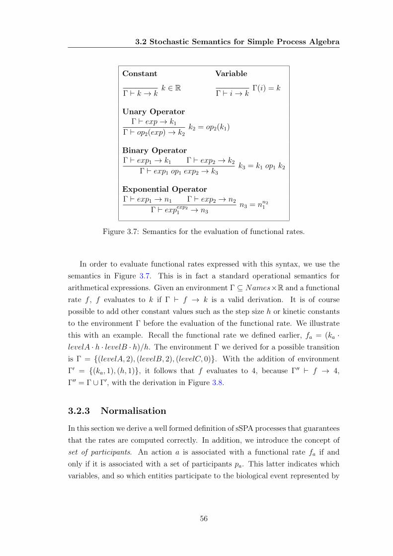
3.2 Stochastic Semantics for Simple Process Algebra
Constant Variable
Γ ` k → kk ∈ R
Γ ` i→ kΓ(i) = k
Unary OperatorΓ ` exp→ k1
Γ ` op2(exp)→ k2
k2 = op2(k1)
Binary OperatorΓ ` exp1 → k1 Γ ` exp2 → k2
Γ ` exp1 op1 exp2 → k3
k3 = k1 op1 k2
Exponential OperatorΓ ` exp1 → n1 Γ ` exp2 → n2
Γ ` expexp2
1 → n3
n3 = nn21
Figure 3.7: Semantics for the evaluation of functional rates.
In order to evaluate functional rates expressed with this syntax, we use the
semantics in Figure 3.7. This is in fact a standard operational semantics for
arithmetical expressions. Given an environment Γ ⊆ Names×R and a functional
rate f , f evaluates to k if Γ ` f → k is a valid derivation. It is of course
possible to add other constant values such as the step size h or kinetic constants
to the environment Γ before the evaluation of the functional rate. We illustrate
this with an example. Recall the functional rate we defined earlier, fa = (ka ·levelA · h · levelB · h)/h. The environment Γ we derived for a possible transition
is Γ = {(levelA, 2), (levelB, 2), (levelC, 0)}. With the addition of environment
Γ′ = {(ka, 1), (h, 1)}, it follows that f evaluates to 4, because Γ′′ ` f → 4,
Γ′′ = Γ ∪ Γ′, with the derivation in Figure 3.8.
3.2.3 Normalisation
In this section we derive a well formed definition of sSPA processes that guarantees
that the rates are computed correctly. In addition, we introduce the concept of
set of participants. An action a is associated with a functional rate fa if and
only if it is associated with a set of participants pa. This latter indicates which
variables, and so which entities participate to the biological event represented by
56
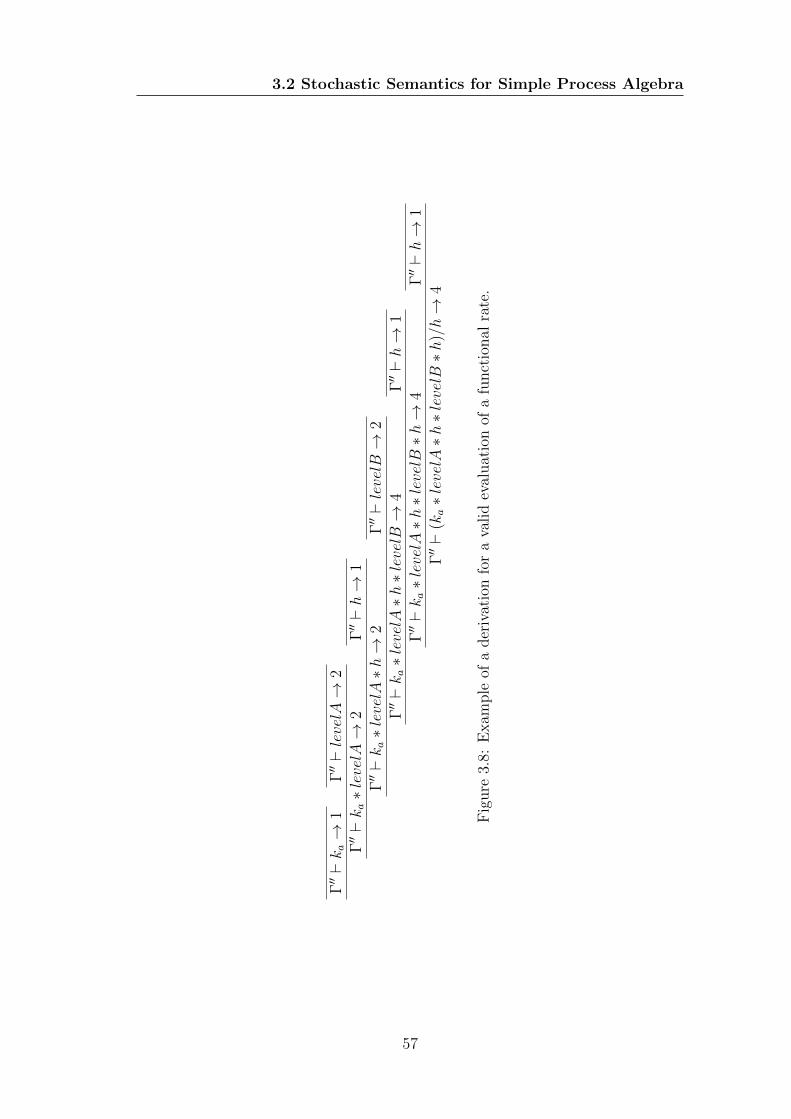
3.2 Stochastic Semantics for Simple Process Algebra
Γ′′`ka→
1Γ′′`levelA→
2Γ′′`ka∗levelA→
2Γ′′`h→
1Γ′′`ka∗levelA∗h→
2Γ′′`levelB→
2Γ′′`ka∗levelA∗h∗levelB→
4Γ′′`h→
1Γ′′`ka∗levelA∗h∗levelB∗h→
4Γ′′`h→
1
Γ′′`
(ka∗levelA∗h∗levelB∗h
)/h→
4
Fig
ure
3.8:
Exam
ple
ofa
der
ivat
ion
for
ava
lid
eval
uat
ion
ofa
funct
ional
rate
.
57
3.2 Stochastic Semantics for Simple Process Algebra
action a. These variables are also sufficient to evaluate fa, though not all of them
may be necessary. In fact, pa is not just the set of variables used to evaluate fa,
it is used to represent the scope of action a, and so to identify if all processes
associated with variables in pa that are assumed to synchronise on a have done so.
This mechanism is the key to the proof of congruence of the equivalence relations
we introduce in Chapter 6.
In some cases the rate ra computed from a functional rate fa associated with
action a is not correct and requires to be scaled. Namely, the rate computed is
divided by the number of actions a a process can perform. This procedure is
referred to as normalisation in (Bernardo, 1996), and usually needs to be applied
when a single rate is associated with multiple actions, a situation often caused
by non deterministic choices. The well formed definition ensures normalisation is
performed correctly and is sound with respect to biological assumptions.
In sSPA as defined so far, we identify two sources of non deterministic choice
that require particular attention, one generated by the + operator and the other
by the BCL
operator. The first type of non deterministic choice always requires
normalisation, while the second type requires normalisation only in some cases
and might interfere with the normalisation of the first. To illustrate this problem
and motivate the solution, consider the following four processes, recalling the
agent definitions of our running example for this section:
1. A′1 BCa (B1 BCaC1)
2. A1 BCa
(B1 BCa
(C1 BC∅ C1))
3. A1 BCa
(B1 BCa
(C1 BC∅ D1))
4. (A1 BC∅ A1)BCa
(B1 BCaC1)
Additional agent definitions and associated variables and values are:
A′1 , a.A0 + a.A2 Var(A′1) = levelA Val(A′1) = 1
D1 , a.D2 Var(D1) = levelD Val(D1) = 1
The current activities of the four processes are:
1. Activities(A′1 BCa (B1 BCaC1)) = {|(a,Γ), (a,Γ)|}
2. Activities(A1 BCa
(B1 BCa
(C1 BC∅ C1))) = {|(a,Γ), (a,Γ)|}
58
3.2 Stochastic Semantics for Simple Process Algebra
3. Activities(A1 BCa
(B1 BCa
(C1 BC∅ D1))) = {|(a,Γ), (a,Γ′)|}
4. Activities((A1 BC∅ A1)BCa
(B1 BCaC1)) = {|(a,Γ), (a,Γ)|}
where Γ = {(levelA, 1), (levelB, 1), (levelC, 1)} and Γ′ = {(levelA, 1),
(levelB, 1), (levelD, 1)}. Recall that the functional rate associated with a is:
fa = (ka · levelA · h · levelB · h)/h
The activities can then be rated using fa and the additional set Γ′′ = {(h, 1),
(ka, 1)}. We can assume (a,Γ) is rated to (a, 1), because Γ ∪ Γ′′ ` fa → 1
and (a,Γ′) is also rated to (a, 1), because Γ′ ∪ Γ′′ ` fa → 1. Thus, assuming
RatedAct(M) is the multi-set of rated activities of process M :
1. RatedAct(A′1 BCa (B1 BCaC1)) = {|(a, 1), (a, 1)|}
2. RatedAct(A1 BCa
(B1 BCa
(C1 BC∅ C1))) = {|(a, 1), (a, 1)|}
3. RatedAct(A1 BCa
(B1 BCa
(C1 BC∅ D1))) = {|(a, 1), (a, 1)|}
4. RatedAct((A1 BC∅ A1)BCa
(B1 BCaC1)) = {|(a, 1), (a, 1)|}
In the case of process 1, the two rated activities (a, 1) and (a, 1) should be
normalised, that is the actual rated activities should be divided by the multiplicity
of (a,Γ), in this case 2. This is because, under the non deterministic choice caused
by the + operator in A′1, we assume that the rate ra evaluated from the functional
rate fa, represents the total exit rate for action a. This assumption is based on the
fact that the two a actions represent two different outcomes of the same biological
event involving the same biological species. Thus, the actual multi-set of rated
activities for process 1 should be:
RatedAct(A′1 BCa (B1 BCaC1)) = {|(a, 0.5), (a, 0.5)|}
If the deterministic choice is generated by the BCL
operator, as in processes 2,
3 and 4, it becomes more complicated to determine whether normalisation should
be applied. It usually depends on what processes and actions represent, and what
functional rate is associated with the actions.
In the case of process 2, the two identical rated activities (a, 1) and (a, 1)
should also be normalised. This is because the non deterministic choice is between
two agents C1 which represent the concentration of biochemical species C, which
59
3.2 Stochastic Semantics for Simple Process Algebra
in turn does not contribute to the determination of the rate. The concentrations of
A and B determine the exit rate for action a, while the produced concentration
of C can be added non deterministically to one of the pools of concentration
represented by the two agents C1. Thus, the actual multi-set of rated activities
for process 2 should be:
RatedAct(A1 BCa
(B1 BCa
(C1 BC∅ C1))) = {|(a, 0.5), (a, 0.5)|}
In the case of process 3, the two rated activities (a, 1) and (a, 1) should also
be normalised. This should be done even if the environment of those activities
differ, as in this case, where one activity has environment Γ, while the other Γ′.
The reason is analogous to that for process 2. The total exit rate is determined
by the concentration of A and B, while the produced concentration can be the
concentration of C or of D. The actual multi-set of rated activities for process 3
should be:
RatedAct(A1 BCa
(B1 BCa
(C1 BC∅ D1))) = {|(a, 0.5), (a, 0.5)|}
In the case of process 4, the two rated activities (a, 1) and (a, 1) should not be
normalised. This is because the non deterministic choice is between two agents
A1 that represent the concentration of biochemical species A, which in turn con-
tributes to the determination of the rate. More precisely, we can observe that
the rate of action a is proportional to the concentration level represented by A1.
Each agent A1 represents a certain “pool” of concentration of species A, which
can interact independently with species B and C. The total concentration of A
present in the system is the sum of the concentration represented by the two
agents A1. Since the rate is proportional to the concentration of A, then the
total exit rate should be given by the sum of the two individual rates.
We have seen that for processes 1, 2, 3 and 4 the multi-set of rated activ-
ities is {|(a, 1), (a, 1)|} if normalisation is not applied. We have also seen that
normalisation is applied only in some cases, which might be difficult to identify.
In particular, without the knowledge of what process performed the actions and
what type of non determinism is involved, we are not able to determine whether
normalisation is necessary or not. In order to have an automatic procedure for
normalisation, we propose that the non-determinism caused by BCL
operator is
not valid. This can be enforced easily if:
60
3.2 Stochastic Semantics for Simple Process Algebra
• in every state of the system there is only one process associated with a
certain variable. This can be ensured by insisting that the initial state
has this property and that for all agents A, whenever A(a,Γ)−−−→ A′ then
Var(A) = Var(A′), conditions that can be tested on the definition of the
model;
• an action a is associated with a set of participants pa ⊆ Names, in this
case pa = {levelA, levelB, levelC}. An activity (a,Γ) can be rated only
if the variables contained in Γ are exactly the variables contained in pa.
This ensures that if there is a non deterministic choice between agents with
different associated variables, only one will be considered a valid choice for
rate evaluation.
With these constraints, it is easy to see that processes 2 and 4 are not well
formed, because they present two processes with the same associated variable,
that is levelC in the first case and levelA in the second. Moreover, in the case
of process 3, activity (a,Γ′) cannot be evaluated to (a, 1) because Γ′ does not
contain exactly the variables contained in pa.
Finally, the use of a set of participants pa raises the question of what happens
if processes associated with variables not in pa synchronise on a. This could have
the effect of turning an activity that can be rated (variables in Γ equal to pa) into
one that cannot be rated. For example, consider the following model process:
5. A1 BCa
(B1 BCa
(C1 BCaD1))
The corresponding set of current activities is:
5. Activities(A1 BCa
(B1 BCa
(C1 BCaD1))) = {|(a,Γ′′)|}
where Γ′′ = {(levelA, 1), (levelB, 1), (levelC, 1), (levelD, 1)}. Activity (a,Γ′′)
cannot be rated, because the variables in Γ′′ are not exactly the variables in
pa. To prevent this situation we add the following constraint:
• if fa is a functional rate in F then a derivative of process P can perform
action a if and only if Var(P ) is in pa.
We can now define an sSPA model and a well formed sSPA model:
Definition 3.9 sSPA model. An sSPA model is a tuple:
61
3.2 Stochastic Semantics for Simple Process Algebra
(AgentDef ,M,Actions,Names,F,Γ, Participants,Var ,Val)
where:
• AgentDef is the finite set of agent definitions {A1 , D1, A2 , D2, . . . };
• M is the initial state of the model, with M ∈ Pm;
• Actions is the finite set of actions;
• Names is the finite set of parameter names;
• F is the finite set of functional rates;
• Γ is the finite set of constant model parameters, with Γ ⊆ Names× R;
• Participants is the finite set of sets of participants;
• Var and Val are the functions associating agents with variables (i.e. pa-
rameter names) and values, with Var : Pm → Names and Val : Pm → R.
Definition 3.10 Well formed sSPA model. An sSPA model is well formed if
and only if:
1. Given a model process as a cooperation of agents, of the form
A1 BCL1A2 BC
L2. . . BC
Ln−1An
then ∀Ai, Aj if i 6= j then Var(Aj) 6= Var(Aj);
2. Given a definition process as a choice of sequential actions, of the form
A ,∑i
ai.Ai
then ∀Ai Var(A) = Var(Ai);
3. ∀a s.t. fa ∈ F
∃(a,Γ) ∈−−−−−−→Activities(P )⇔ Var(P ) ∈ pa
62
3.2 Stochastic Semantics for Simple Process Algebra
3.2.4 The Rating Routines
In the previous sections we have defined how to evaluate a functional rate f
using the environment Γ of an activity and an additional constant environment
Γ′. In this section we define a mechanism to determine when it is appropriate to
evaluate a functional rate and we determine what happens when an evaluation
is not possible. The result is a rating procedure that converts a derivation graph
(Definition 3.8) into a rated derivation graph.
Recall again our running example. If we consider a model composed only of
process A2, the following derivation is valid:
A2(a,{(levelA,2)})−−−−−−−−−→ A1
Given the above transition and the functional rate fa associated with action
a, it is clear that an evaluation of fa is not possible. In fact, environment Γ =
{(levelA, 2)} is missing variable levelB. In this case, we call the transition and
the activity (a,Γ) open.
Now consider the following transition:
A2 BCaB2
(a,Γ′)−−−→ A1 BCaB1
where Γ′ = {(levelA, 2), (levelB, 2)}. In this case, fa can be evaluated correctly,
because all the necessary variables are included in Γ′. However, we consider this
transition open as well and we do not allow the functional rate to be evaluated
just yet. This is because not all the processes that will be affected by the action
synchronise on a.
Formally, we consider the list of participants of action a, pa = {levelA, levelB,levelC}. Participants are variables required for the evaluation of the rate to be
successful. These may not only be variables whose values we need to know in
order to evaluate the rate, but also variables associated with elements that will
be affected by the reaction.
The concept of participants of an action has an important role in our ap-
proach to functional rates. Later on we will show how we exploit this concept
in compositionality (Section 6). Intuitively, we use the list of participants to
indicate exactly which processes will synchronise on a certain action. Once the
environment Γ collected from the execution of action a contains all the variables
in pa, fa can be evaluated and we assume no further processes will synchronise.
63
3.2 Stochastic Semantics for Simple Process Algebra
This is a quite strong assumption and it is based on the observation that, at least
in biology, one should always be able to identify which elements in a system are
affected by a certain event.
Finally, we know that some transitions can be turned into rated transitions,
while others cannot. This implies that the derivation graph resulting after the
rating operation will include two types of transitions, open transitions and rated
transitions.
We proceed now to the formalisation of the procedure used to rate activities
and the definition of a rated derivation graph.
Definition 3.11 Function envVar. The function envVar extracts the set of
variables in an environment Γ ⊆ Names× R:
envV ar(Γ) = ({i | (i, k) ∈ Γ})
Definition 3.12 Open activity. An open activity is an activity (a,Γ) where Γ
does not contain the exact variables present in the participant set pa, i.e. pa 6=envV ar(Γ).
Definition 3.13 Function openActivities. The function openActivities selects
open activities from a set of activities A ⊆ Actions× 2Names×R:
openActivities(A) =
({|(a,Γ) | pa 6= envV ar(Γ) ∧ (a,Γ) ∈ A |}
)
Definition 3.14 Current open activities. Given a model process M ∈ Pm, the
set of open activities that P can perform is defined as:
OpenAct(M) = openActivities(Activities(M))
Definition 3.15 Open activity set. The set of all open activities that a model
process M ∈ Pm can perform is given by:
−−−−−−→OpenAct(M) = openActivities(
−−−−−−→Activities(M))
64
3.2 Stochastic Semantics for Simple Process Algebra
Definition 3.16 Closed activity. A closed activity is an activity (a,Γ) where Γ
contains the exact variables present in the participant set pa, i.e. pa = envV ar(Γ).
Definition 3.17 Function closedActivities. The function closedActivities selects
closed activities from a set of activities A ⊆ Actions× 2Names×R:
closedActivities(A) = (A \ openActivities(A))
Definition 3.18 Current closed activities. Given a model process M ∈ Pm, the
set of closed activities that M can perform is defined as:
ClosedAct(M) = closedActivities(Activities(M))
Definition 3.19 Closed activity set. The set of all open activities that a model
process M ∈ Pm can perform is given by:
−−−−−−−→ClosedAct(M) = closedActivities(
−−−−−−→Activities(M))
Definition 3.20 Rated activity. The pair (a, r) such that a ∈ Actions and
r ∈ R>0 is called a rated activity.
Definition 3.21 Function rateActivities. Given an environment Γ, rateActivi-
ties converts a set of activities A ⊆ Actions×2Names×R into a set of rated activities
B ⊆ Actions× R:
rateActivities(Γ)(A) =
{|(a, ra) | Γ ∪ Γ′ ` fa → k ∧ ra = k/π(A, (a,Γ′)) ∧ (a,Γ′) ∈ A ∧ fa ∈ F |}
where π(A, (a,Γ′)) returns the number of occurrences of (a,Γ′) in the multi-set
A.
Definition 3.22 Current rated activities. Given a model process M ∈ Pm and
an environment Γ ⊆ Names× R, the set of rated activities that M can perform
is defined as:
RatedAct(M)Γ = rateActivities(Γ)(ClosedAct(M))
65
3.2 Stochastic Semantics for Simple Process Algebra
RatedAct(M)Γ can be written RatedAct(M) if Γ is clear from the context.
Definition 3.23 Rated activity set. Given an environment Γ ⊆ Names× R,
the set of all rated activities that a model process M ∈ Pm can perform is given
by:−−−−−−→RatedAct(M)Γ = rateActivity(Γ)(
−−−−−−−→ClosedAct(M))
−−−−−−→RatedAct(M)Γ can be written
−−−−−−→RatedAct(M) if Γ is clear from the context.
Definition 3.24 Rated derivation graph. Given a model process M ∈ Pm and an
environment Γ ⊆ Names× R, the rated derivation graph Dr(M)Γ is the labelled
directed graph with:
• set of nodes ds(M);
• multi-set of transition labels−−−−−−→RatedAct(M)Γ;
• multi-set of labelled transitions →r⊆ ds(M) ×−−−−−−→RatedAct(M)Γ × ds(M).
Given M ′ ∈ ds(M), (M ′, a, ra,M′′) ∈→r iff M ′ (a,Γ′)−−−→ M ′′, (a,Γ′) ∈
ClosedAct(M) and {|(a, k)|} = rateActivities(Γ)({|(a,Γ′)|}) and ra
= k/π(ClosedAct(M), (a,Γ′)).
• multi-set of labelled transitions→o⊆ ds(M)×−−−−−−→OpenAct(M)×ds(M). Given
M ′ ∈ ds(M), (M ′, a,Γ′,M ′′) ∈→o iffM ′ (a,Γ′)−−−→M ′′ and (a,Γ′) ∈ OpenAct(M).
Dr(M)Γ can be written Dr(M) if Γ is clear from the context.
The rated derivation graph of the running example of Section 3.2,
Dr(A2 BCa
(B2 BCaC0))Γ, with Γ = {(ka, 1), (h, 1)}, is:
A2 BCa
(B2 BCaC0)
(a,4)−−→ A1 BCa
(B1 BCaC1)
(a,1)−−→ A0 BCa
(B0 BCaC2)
3.2.5 Stochastic Simple Process Algebra and Tissue Growth
We return now to the example we introduced in Section 3.1.2, with the addition
of functional rates. In particular, we associate a constant rate kapo to apoptosis,
i.e. tissue death, and a rate kmito to mitosis, i.e. tissue replication. In order
to demonstrate that a rate can depend on the current state of the system, we
assume that kmito is the total rate of mitosis of a region containing tissue, that
66
3.2 Stochastic Semantics for Simple Process Algebra
is the sum of the rates of all mitosis actions from that region. This implies that
functional rates of mitosis actions depend on whether adjacent regions contain
tissue or not.
The definition of the processes is:
Empty0 , mito10.Tissue0 + mito12.Empty0
Empty1 , mito01.Tissue1 + mito21.Tissue1
Empty2 , mito12.Tissue2 + mito10.Empty2
Tissue0 , apo0.Empty0 + mito01.Tissue0 + mito12.Tissue0
Tissue1 , apo1.Empty1 + mito10.Tissue1 + mito12.Tissue1
Tissue2 , apo2.Empty2 + mito21.Tissue2 + mito10.Tissue2
The initial state of the model is defined by the following process:
Empty0BCL
Tissue1BCK
Empty2
where L = {mito10,mito01} and K = {mito12,mito21}. Variables and values
associated to processes are:
Var(Empty0) = Var(Tissue0) = region0 Val(Empty0) = 0 Val(Tissue0) = 1
Var(Empty1) = Var(Tissue1) = region1 Val(Empty1) = 0 Val(Tissue1) = 1
Var(Empty2) = Var(Tissue2) = region2 Val(Empty2) = 0 Val(Tissue2) = 1
Functional rates and sets of participants are defined as:
fmito01 = kmito pmito01 = {region0, region1}
fmito12 = kmito/(2− region0) pmito12 = {region0, region1, region2}
fmito21 = kmito pmito21 = {region2, region1}
fmito10 = kmito/(2− region2) pmito10 = {region0, region1, region2}
fapo0 = kapo papo0 = {region0}
fapo1 = kapo papo1 = {region1}
fapo2 = kapo papo2 = {region2}
For example, fmito12 implies that if region R0 is empty then the rate for mito12
has to be divided by 2. The case is analogous for fmito10. As a consequence
Tissue1 performs mitosis always at a total rate of kmito .
Examples of valid derivations are:
67
3.3 Parametric Simple Process Algebra
Empty0BCL
Tissue1BCK
Empty2(apo1,Γ)−−−−→ Empty0BC
LEmpty1BC
KEmpty2
Empty0BCL
Tissue1BCK
Empty2(mito12,Γ′)−−−−−−→ Empty0BC
LTissue1BC
KTissue2
where Γ = {(region1, 1)} and Γ′ = {(region0, 0), (region1, 1), (region2, 0)}. Us-
ing the additional environment Γ′′ = {(kmito , 1), (kapo , 2)}, the transitions can be
rated yielding:
Empty0BCL
Tissue1BCK
Empty2(apo1,2)−−−−→ Empty0BC
LEmpty1BC
KEmpty2
Empty0BCL
Tissue1BCK
Empty2(mito12,0.5)−−−−−−−→ Empty0BC
LTissue1BC
KTissue2
3.3 Parametric Simple Process Algebra
We have seen in several examples so far that model definitions tend to be repet-
itive when modelling levels of concentration or entities located in space. In this
section we show how the description of a model written in SPA can be reduced
by the introduction of parameters and an “if then else” construct.
The syntax of the parametric simple process algebra with multi-way synchro-
nisation (pSPA) is:
P ::= nil | a(exp, . . . , exp).P | P + P | P BCLP | [bexp]?P : P | A(exp, . . . , exp)
exp ::= k | i | exp+ exp | exp− exp | exp/k′
bexp ::= exp = exp | exp < exp | bexp ∧ bexp | bexp ∨ bexp | ¬bexp | true | false
where:
• P is a process, P ∈ P, with P the set of processes;
• nil is the deadlock process;
• a is an action, a ∈ Actions, with Actions the set of actions;
• exp1, . . . , expn is a non empty list of expressions;
• exp is an expression, which can be an real number k, k ∈ R, a sum of
two expressions, a difference between two expressions, a division between
an expression and an real number k′ ∈ (R \ {0}), the parameter name
i ∈ Names;
68
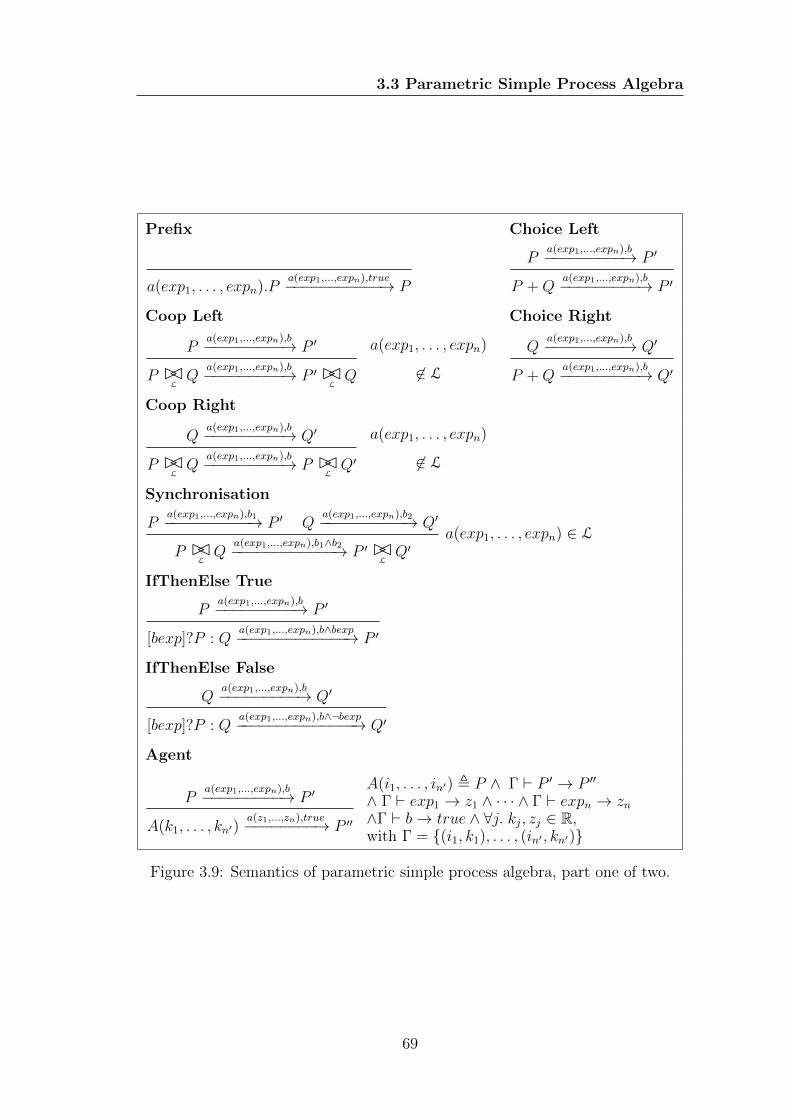
3.3 Parametric Simple Process Algebra
Prefix Choice Left
a(exp1, . . . , expn).Pa(exp1,...,expn),true−−−−−−−−−−−→ P
Pa(exp1,...,expn),b−−−−−−−−−→ P ′
P +Qa(exp1,...,expn),b−−−−−−−−−→ P ′
Coop Left Choice Right
Pa(exp1,...,expn),b−−−−−−−−−→ P ′
P BCLQ
a(exp1,...,expn),b−−−−−−−−−→ P ′ BCLQ
a(exp1, . . . , expn)
6∈ L
Qa(exp1,...,expn),b−−−−−−−−−→ Q′
P +Qa(exp1,...,expn),b−−−−−−−−−→ Q′
Coop Right
Qa(exp1,...,expn),b−−−−−−−−−→ Q′
P BCLQ
a(exp1,...,expn),b−−−−−−−−−→ P BCLQ′
a(exp1, . . . , expn)
6∈ L
Synchronisation
Pa(exp1,...,expn),b1−−−−−−−−−−→ P ′ Q
a(exp1,...,expn),b2−−−−−−−−−−→ Q′
P BCLQ
a(exp1,...,expn),b1∧b2−−−−−−−−−−−−→ P ′ BCLQ′
a(exp1, . . . , expn) ∈ L
IfThenElse True
Pa(exp1,...,expn),b−−−−−−−−−→ P ′
[bexp]?P : Qa(exp1,...,expn),b∧bexp−−−−−−−−−−−−−→ P ′
IfThenElse False
Qa(exp1,...,expn),b−−−−−−−−−→ Q′
[bexp]?P : Qa(exp1,...,expn),b∧¬bexp−−−−−−−−−−−−−−→ Q′
Agent
Pa(exp1,...,expn),b−−−−−−−−−→ P ′
A(k1, . . . , kn′)a(z1,...,zn),true−−−−−−−−→ P ′′
A(i1, . . . , in′) , P ∧ Γ ` P ′ → P ′′
∧ Γ ` exp1 → z1 ∧ · · · ∧ Γ ` expn → zn∧Γ ` b→ true ∧ ∀j. kj, zj ∈ R,with Γ = {(i1, k1), . . . , (in′ , kn′)}
Figure 3.9: Semantics of parametric simple process algebra, part one of two.
69
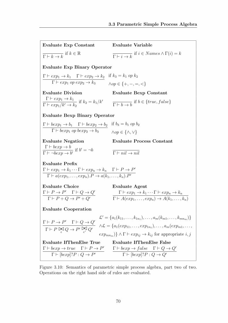
3.3 Parametric Simple Process Algebra
Evaluate Exp Constant Evaluate Variable
Γ ` k → kif k ∈ R
Γ ` i→ kif i ∈ Names ∧ Γ(i) = k
Evaluate Exp Binary Operator
Γ ` exp1 → k1 Γ ` exp2 → k2
Γ ` exp1 op exp2 → k3
if k3 = k1 op k2
∧op ∈ {+,−,=, <}
Evaluate Division Evaluate Bexp ConstantΓ ` exp1 → k1
Γ ` exp1/k′ → k2
if k2 = k1/k′
Γ ` b→ bif b ∈ {true, false}
Evaluate Bexp Binary Operator
Γ ` bexp1 → b1 Γ ` bexp2 → b2
Γ ` bexp1 op bexp2 → b3
if b3 = b1 op b2
∧op ∈ {∧,∨}
Evaluate Negation Evaluate Process ConstantΓ ` bexp→ b
Γ ` ¬bexp→ b′if b′ = ¬b
Γ ` nil→ nil
Evaluate Prefix
Γ ` exp1 → k1 · · ·Γ ` expn → kn Γ ` P → P ′
Γ ` a(exp1, . . . , expn).P → a(k1, . . . , kn).P ′
Evaluate Choice Evaluate Agent
Γ ` P → P ′ Γ ` Q→ Q′
Γ ` P +Q→ P ′ +Q′Γ ` exp1 → k1 · · ·Γ ` expn → kn
Γ ` A(exp1, . . . , expn)→ A(k1, . . . , kn)
Evaluate Cooperation
Γ ` P → P ′ Γ ` Q→ Q′
Γ ` P BCLQ→ P ′ BC
L′Q′
L′ = {a1(k11, . . . , k1n1), . . . , am(km1, . . . , kmnm)}
∧L = {a1(exp11, . . . , exp1n1), . . . , am(expm1, . . . ,
expmnm)} ∧ Γ ` expij → kij for appropriate i, j
Evaluate IfThenElse True Evaluate IfThenElse False
Γ ` bexp→ true Γ ` P → P ′
Γ ` [bexp]?P : Q→ P ′Γ ` bexp→ false Γ ` Q→ Q′
Γ ` [bexp]?P : Q→ Q′
Figure 3.10: Semantics of parametric simple process algebra, part two of two.Operations on the right hand side of rules are evaluated.
70
3.3 Parametric Simple Process Algebra
• a(exp1, . . . , expn) is a parametric action, a(exp1, . . . , expn) ∈ Pactions,
with Pactions the set of parametric actions and exp1, . . . , expn a non empty
list of expressions;
• a(exp1, . . . , expn).P expresses the fact that parametric action a(exp1, . . . , expn)
has to be performed in order to change process a(exp1, . . . , expn).P into the
new process P ;
• P + P expresses the non deterministic choice between two processes. Once
one is chosen, the other is discarded;
• P BCLP expresses the cooperation between two independent processes via
the cooperation set L, with L ⊆ Pactions;
• bexp is a boolean expression, defined as the constant true or false, the
equality test of expressions exp1 = exp2, the “less than” test exp1 < exp2,
the conjunction or disjunction of two boolean expressions or the negation
of a boolean expression;
• [bexp]?P : Q corresponds to P if the evaluation of bexp returns true or Q if
it returns false;
• A(exp1, . . . , expn) is used to recursively define processes, via the agent def-
inition A(i1, . . . , in) , P , with i1, . . . , in ∈ Names and n ∈ (N \ {0}).
The semantics of pSPA is shown in Figures 3.9 and 3.10. The use of parameters
may reduce significantly the length of the description of a process algebra model.
In following two sections we illustrate the use of parameters in two examples.
We will come back to parameters when we introduce the syntax used for the
implementation of process algebra with hooks in Section 7.
3.3.1 Parametric Simple Process Algebra and Biochem-
istry
We now rewrite process definitions for the example in Section 3.1.1 using pSPA.
In particular, we can use the notation A(1, 2) to indicate the concentration of
species A in location 1 is 2.
71
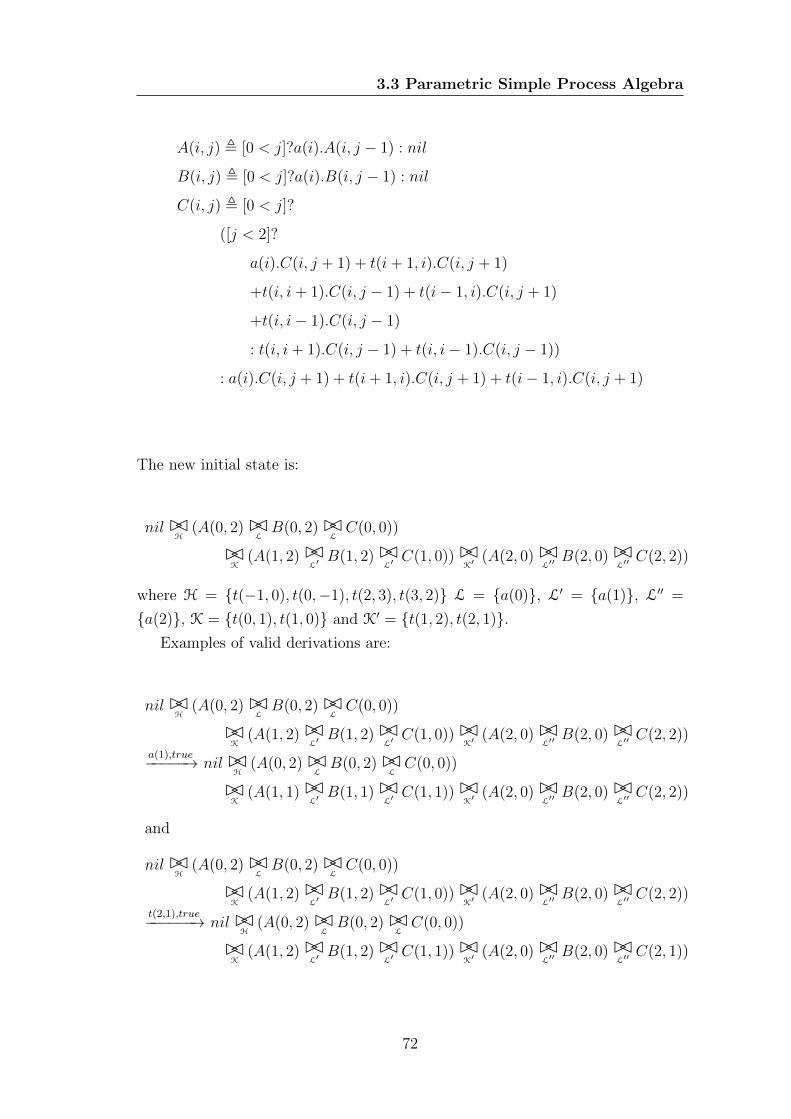
3.3 Parametric Simple Process Algebra
A(i, j) , [0 < j]?a(i).A(i, j − 1) : nil
B(i, j) , [0 < j]?a(i).B(i, j − 1) : nil
C(i, j) , [0 < j]?
([j < 2]?
a(i).C(i, j + 1) + t(i+ 1, i).C(i, j + 1)
+t(i, i+ 1).C(i, j − 1) + t(i− 1, i).C(i, j + 1)
+t(i, i− 1).C(i, j − 1)
: t(i, i+ 1).C(i, j − 1) + t(i, i− 1).C(i, j − 1))
: a(i).C(i, j + 1) + t(i+ 1, i).C(i, j + 1) + t(i− 1, i).C(i, j + 1)
The new initial state is:
nil BCH
(A(0, 2)BCLB(0, 2)BC
LC(0, 0))
BCK
(A(1, 2)BCL′B(1, 2)BC
L′C(1, 0))BC
K′(A(2, 0)BC
L′′B(2, 0)BC
L′′C(2, 2))
where H = {t(−1, 0), t(0,−1), t(2, 3), t(3, 2)} L = {a(0)}, L′ = {a(1)}, L′′ =
{a(2)}, K = {t(0, 1), t(1, 0)} and K′ = {t(1, 2), t(2, 1)}.Examples of valid derivations are:
nil BCH
(A(0, 2)BCLB(0, 2)BC
LC(0, 0))
BCK
(A(1, 2)BCL′B(1, 2)BC
L′C(1, 0))BC
K′(A(2, 0)BC
L′′B(2, 0)BC
L′′C(2, 2))
a(1),true−−−−−→ nil BCH
(A(0, 2)BCLB(0, 2)BC
LC(0, 0))
BCK
(A(1, 1)BCL′B(1, 1)BC
L′C(1, 1))BC
K′(A(2, 0)BC
L′′B(2, 0)BC
L′′C(2, 2))
and
nil BCH
(A(0, 2)BCLB(0, 2)BC
LC(0, 0))
BCK
(A(1, 2)BCL′B(1, 2)BC
L′C(1, 0))BC
K′(A(2, 0)BC
L′′B(2, 0)BC
L′′C(2, 2))
t(2,1),true−−−−−−→ nil BCH
(A(0, 2)BCLB(0, 2)BC
LC(0, 0))
BCK
(A(1, 2)BCL′B(1, 2)BC
L′C(1, 1))BC
K′(A(2, 0)BC
L′′B(2, 0)BC
L′′C(2, 1))
72
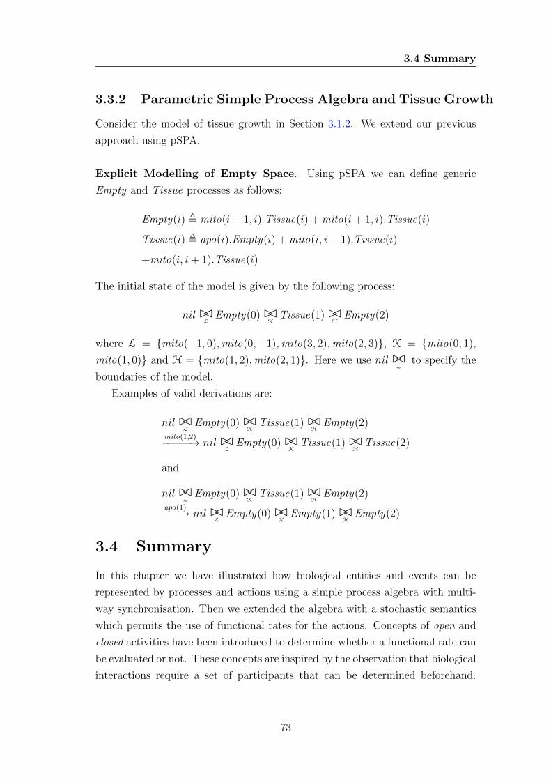
3.4 Summary
3.3.2 Parametric Simple Process Algebra and Tissue Growth
Consider the model of tissue growth in Section 3.1.2. We extend our previous
approach using pSPA.
Explicit Modelling of Empty Space. Using pSPA we can define generic
Empty and Tissue processes as follows:
Empty(i) , mito(i− 1, i).Tissue(i) + mito(i+ 1, i).Tissue(i)
Tissue(i) , apo(i).Empty(i) + mito(i, i− 1).Tissue(i)
+mito(i, i+ 1).Tissue(i)
The initial state of the model is given by the following process:
nil BCL
Empty(0)BCK
Tissue(1)BCH
Empty(2)
where L = {mito(−1, 0),mito(0,−1),mito(3, 2),mito(2, 3)}, K = {mito(0, 1),
mito(1, 0)} and H = {mito(1, 2),mito(2, 1)}. Here we use nil BCL
to specify the
boundaries of the model.
Examples of valid derivations are:
nil BCL
Empty(0)BCK
Tissue(1)BCH
Empty(2)mito(1,2)−−−−−→ nil BC
LEmpty(0)BC
KTissue(1)BC
HTissue(2)
and
nil BCL
Empty(0)BCK
Tissue(1)BCH
Empty(2)apo(1)−−−→ nil BC
LEmpty(0)BC
KEmpty(1)BC
HEmpty(2)
3.4 Summary
In this chapter we have illustrated how biological entities and events can be
represented by processes and actions using a simple process algebra with multi-
way synchronisation. Then we extended the algebra with a stochastic semantics
which permits the use of functional rates for the actions. Concepts of open and
closed activities have been introduced to determine whether a functional rate can
be evaluated or not. These concepts are inspired by the observation that biological
interactions require a set of participants that can be determined beforehand.
73

3.4 Summary
Finally, we defined a parametrised version of the simple process algebra, to reduce
the length of model definitions. Several examples using simple process algebra
and its extensions have been given throughout the chapter.
In the next chapter we address the problem of modelling multiple spatial scales
and the interactions within and between spatial scales.
74
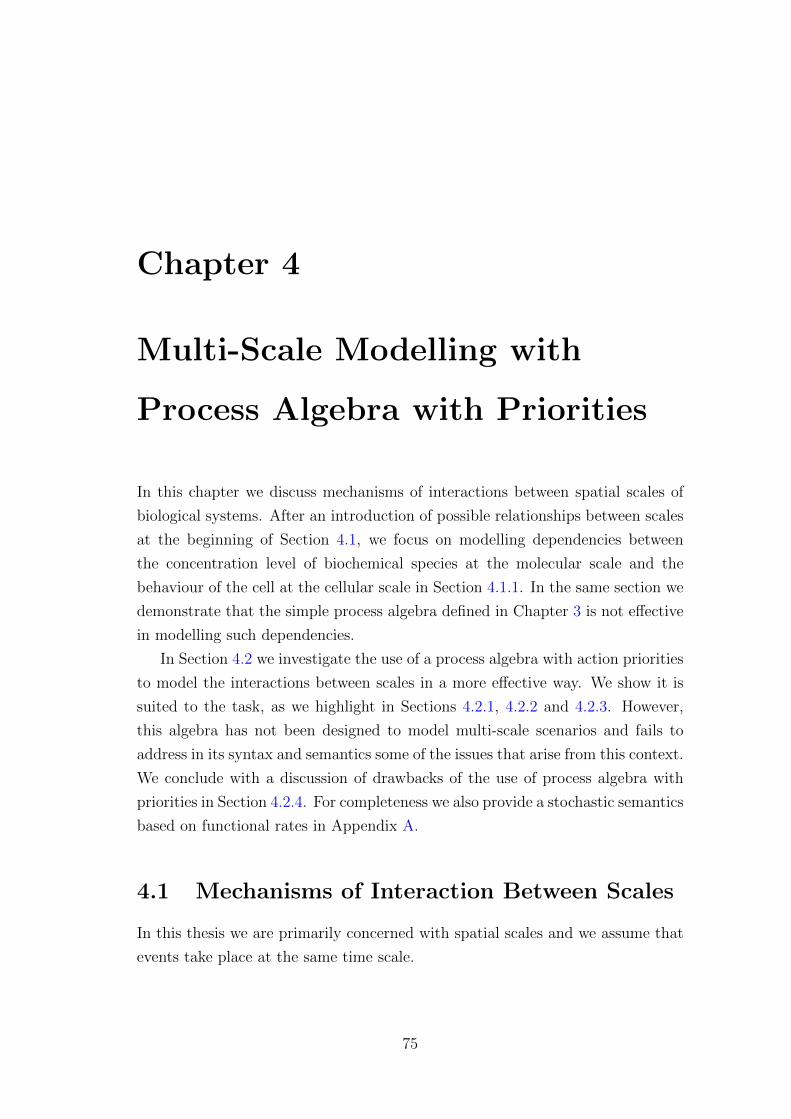
Chapter 4
Multi-Scale Modelling with
Process Algebra with Priorities
In this chapter we discuss mechanisms of interactions between spatial scales of
biological systems. After an introduction of possible relationships between scales
at the beginning of Section 4.1, we focus on modelling dependencies between
the concentration level of biochemical species at the molecular scale and the
behaviour of the cell at the cellular scale in Section 4.1.1. In the same section we
demonstrate that the simple process algebra defined in Chapter 3 is not effective
in modelling such dependencies.
In Section 4.2 we investigate the use of a process algebra with action priorities
to model the interactions between scales in a more effective way. We show it is
suited to the task, as we highlight in Sections 4.2.1, 4.2.2 and 4.2.3. However,
this algebra has not been designed to model multi-scale scenarios and fails to
address in its syntax and semantics some of the issues that arise from this context.
We conclude with a discussion of drawbacks of the use of process algebra with
priorities in Section 4.2.4. For completeness we also provide a stochastic semantics
based on functional rates in Appendix A.
4.1 Mechanisms of Interaction Between Scales
In this thesis we are primarily concerned with spatial scales and we assume that
events take place at the same time scale.
75
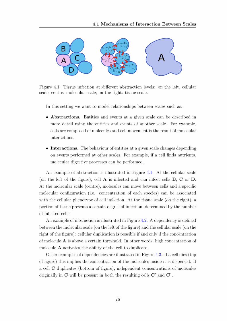
4.1 Mechanisms of Interaction Between Scales
A
BC
D
A B
CDA B
CD
A B
CD
A B
CD
A B
CD
A B
CD A
Figure 4.1: Tissue infection at different abstraction levels: on the left, cellularscale; centre: molecular scale; on the right: tissue scale.
In this setting we want to model relationships between scales such as:
• Abstractions. Entities and events at a given scale can be described in
more detail using the entities and events of another scale. For example,
cells are composed of molecules and cell movement is the result of molecular
interactions.
• Interactions. The behaviour of entities at a given scale changes depending
on events performed at other scales. For example, if a cell finds nutrients,
molecular digestive processes can be performed.
An example of abstraction is illustrated in Figure 4.1. At the cellular scale
(on the left of the figure), cell A is infected and can infect cells B, C or D.
At the molecular scale (centre), molecules can move between cells and a specific
molecular configuration (i.e. concentration of each species) can be associated
with the cellular phenotype of cell infection. At the tissue scale (on the right), a
portion of tissue presents a certain degree of infection, determined by the number
of infected cells.
An example of interaction is illustrated in Figure 4.2. A dependency is defined
between the molecular scale (on the left of the figure) and the cellular scale (on the
right of the figure): cellular duplication is possible if and only if the concentration
of molecule A is above a certain threshold. In other words, high concentration of
molecule A activates the ability of the cell to duplicate.
Other examples of dependencies are illustrated in Figure 4.3. If a cell dies (top
of figure) this implies the concentration of the molecules inside it is dispersed. If
a cell C duplicates (bottom of figure), independent concentrations of molecules
originally in C will be present in both the resulting cells C’ and C”.
76
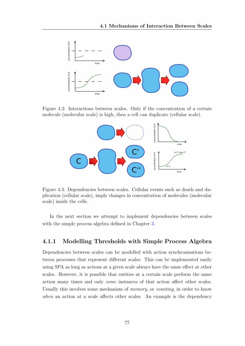
4.1 Mechanisms of Interaction Between Scales
Figure 4.2: Interactions between scales. Only if the concentration of a certainmolecule (molecular scale) is high, then a cell can duplicate (cellular scale).
CC'
C''
Figure 4.3: Dependencies between scales. Cellular events such as death and du-plication (cellular scale), imply changes in concentration of molecules (molecularscale) inside the cells.
In the next section we attempt to implement dependencies between scales
with the simple process algebra defined in Chapter 3.
4.1.1 Modelling Thresholds with Simple Process Algebra
Dependencies between scales can be modelled with action synchronisations be-
tween processes that represent different scales. This can be implemented easily
using SPA as long as actions at a given scale always have the same effect at other
scales. However, it is possible that entities at a certain scale perform the same
action many times and only some instances of that action affect other scales.
Usually this involves some mechanism of memory, or counting, in order to know
when an action at a scale affects other scales. An example is the dependency
77
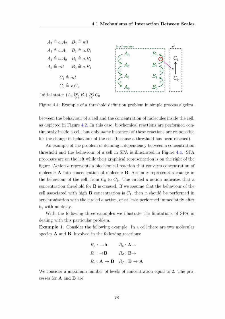
4.1 Mechanisms of Interaction Between Scales
A3 , a.A2 B3 , nil
A2 , a.A1 B2 , a.B3
A1 , a.A0 B1 , a.B2
A0 , nil B0 , a.B1
C1 , nil
C0 , x.C1
Initial state: (A3 BC{a} B0)BC{x}
C0
Figure 4.4: Example of a threshold definition problem in simple process algebra.
between the behaviour of a cell and the concentration of molecules inside the cell,
as depicted in Figure 4.2. In this case, biochemical reactions are performed con-
tinuously inside a cell, but only some instances of these reactions are responsible
for the change in behaviour of the cell (because a threshold has been reached).
An example of the problem of defining a dependency between a concentration
threshold and the behaviour of a cell in SPA is illustrated in Figure 4.4. SPA
processes are on the left while their graphical representation is on the right of the
figure. Action a represents a biochemical reaction that converts concentration of
molecule A into concentration of molecule B. Action x represents a change in
the behaviour of the cell, from C0 to C1. The circled a action indicates that a
concentration threshold for B is crossed. If we assume that the behaviour of the
cell associated with high B concentration is C1, then x should be performed in
synchronisation with the circled a action, or at least performed immediately after
it, with no delay.
With the following three examples we illustrate the limitations of SPA in
dealing with this particular problem.
Example 1. Consider the following example. In a cell there are two molecular
species A and B, involved in the following reactions:
Ra : →A Rb : A→
Rc : →B Rd : B→
Re : A → B Rf : B → A
We consider a maximum number of levels of concentration equal to 2. The pro-
cesses for A and B are:
78
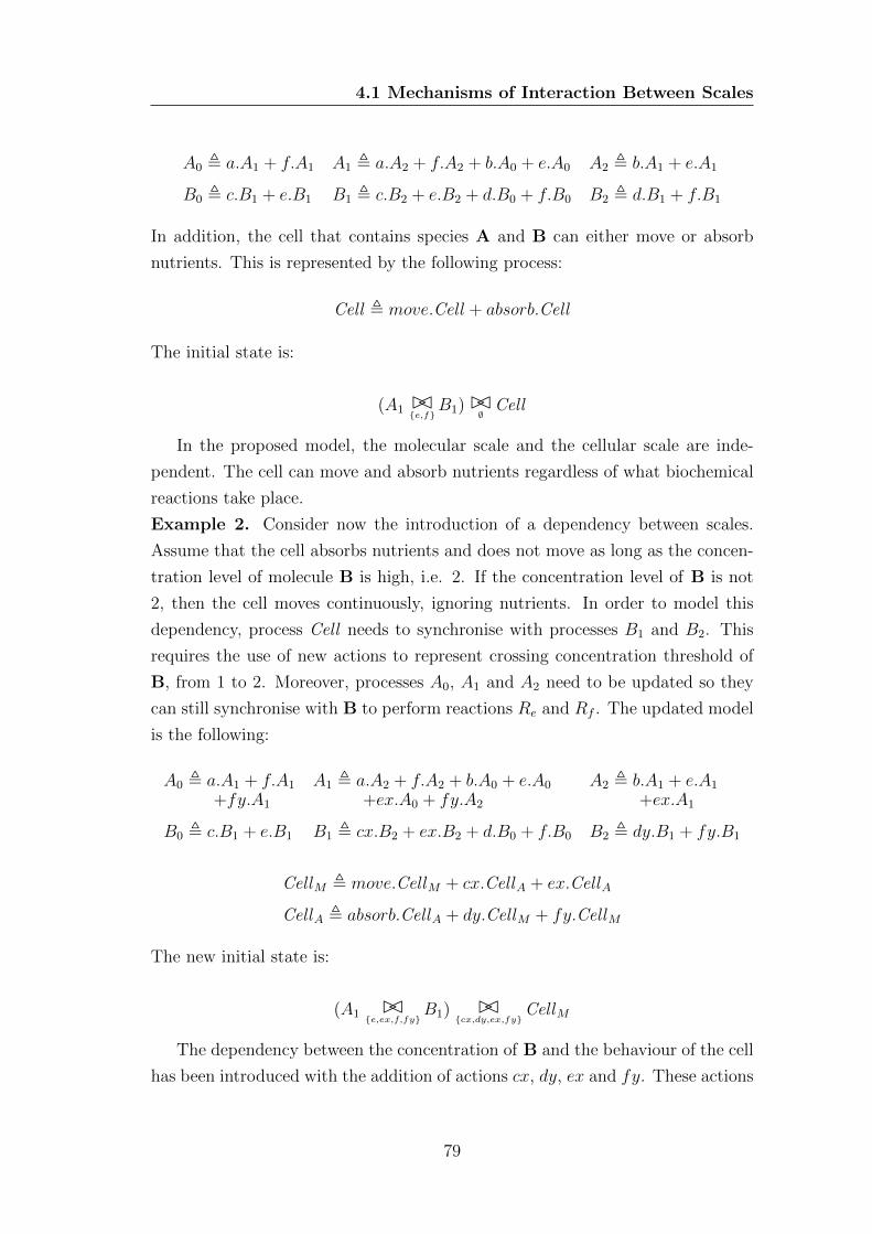
4.1 Mechanisms of Interaction Between Scales
A0 , a.A1 + f.A1 A1 , a.A2 + f.A2 + b.A0 + e.A0 A2 , b.A1 + e.A1
B0 , c.B1 + e.B1 B1 , c.B2 + e.B2 + d.B0 + f.B0 B2 , d.B1 + f.B1
In addition, the cell that contains species A and B can either move or absorb
nutrients. This is represented by the following process:
Cell , move.Cell + absorb.Cell
The initial state is:
(A1 BC{e,f}B1)BC∅
Cell
In the proposed model, the molecular scale and the cellular scale are inde-
pendent. The cell can move and absorb nutrients regardless of what biochemical
reactions take place.
Example 2. Consider now the introduction of a dependency between scales.
Assume that the cell absorbs nutrients and does not move as long as the concen-
tration level of molecule B is high, i.e. 2. If the concentration level of B is not
2, then the cell moves continuously, ignoring nutrients. In order to model this
dependency, process Cell needs to synchronise with processes B1 and B2. This
requires the use of new actions to represent crossing concentration threshold of
B, from 1 to 2. Moreover, processes A0, A1 and A2 need to be updated so they
can still synchronise with B to perform reactions Re and Rf . The updated model
is the following:
A0 , a.A1 + f.A1 A1 , a.A2 + f.A2 + b.A0 + e.A0 A2 , b.A1 + e.A1
+fy.A1 +ex.A0 + fy.A2 +ex.A1
B0 , c.B1 + e.B1 B1 , cx.B2 + ex.B2 + d.B0 + f.B0 B2 , dy.B1 + fy.B1
CellM , move.CellM + cx.CellA + ex.CellA
CellA , absorb.CellA + dy.CellM + fy.CellM
The new initial state is:
(A1 BC{e,ex,f,fy}
B1) BC{cx,dy,ex,fy}
CellM
The dependency between the concentration of B and the behaviour of the cell
has been introduced with the addition of actions cx, dy, ex and fy. These actions
79
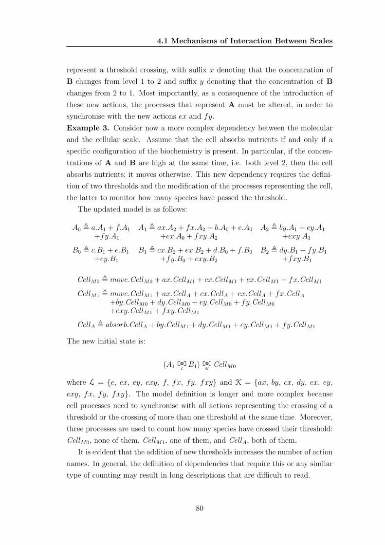
4.1 Mechanisms of Interaction Between Scales
represent a threshold crossing, with suffix x denoting that the concentration of
B changes from level 1 to 2 and suffix y denoting that the concentration of B
changes from 2 to 1. Most importantly, as a consequence of the introduction of
these new actions, the processes that represent A must be altered, in order to
synchronise with the new actions ex and fy.
Example 3. Consider now a more complex dependency between the molecular
and the cellular scale. Assume that the cell absorbs nutrients if and only if a
specific configuration of the biochemistry is present. In particular, if the concen-
trations of A and B are high at the same time, i.e. both level 2, then the cell
absorbs nutrients; it moves otherwise. This new dependency requires the defini-
tion of two thresholds and the modification of the processes representing the cell,
the latter to monitor how many species have passed the threshold.
The updated model is as follows:
A0 , a.A1 + f.A1 A1 , ax.A2 + fx.A2 + b.A0 + e.A0 A2 , by.A1 + ey.A1
+fy.A1 +ex.A0 + fxy.A2 +exy.A1
B0 , c.B1 + e.B1 B1 , cx.B2 + ex.B2 + d.B0 + f.B0 B2 , dy.B1 + fy.B1
+ey.B1 +fy.B0 + exy.B2 +fxy.B1
CellM0 , move.CellM0 + ax.CellM1 + cx.CellM1 + ex.CellM1 + fx.CellM1
CellM1 , move.CellM1 + ax.CellA + cx.CellA + ex.CellA + fx.CellA+by.CellM0 + dy.CellM0 + ey.CellM0 + fy.CellM0
+exy.CellM1 + fxy.CellM1
CellA , absorb.CellA + by.CellM1 + dy.CellM1 + ey.CellM1 + fy.CellM1
The new initial state is:
(A1 BCLB1)BC
KCellM0
where L = {e, ex, ey, exy, f, fx, fy, fxy} and K = {ax, by, cx, dy, ex, ey,exy, fx, fy, fxy}. The model definition is longer and more complex because
cell processes need to synchronise with all actions representing the crossing of a
threshold or the crossing of more than one threshold at the same time. Moreover,
three processes are used to count how many species have crossed their threshold:
CellM0, none of them, CellM1, one of them, and CellA, both of them.
It is evident that the addition of new thresholds increases the number of action
names. In general, the definition of dependencies that require this or any similar
type of counting may result in long descriptions that are difficult to read.
80

4.2 Process Algebra with Priorities
As a solution to this problem we propose to employ a process algebra with
action priorities instead of SPA. In the next section we investigate this approach.
4.2 Process Algebra with Priorities
The syntax for a process algebra with multi-way synchronisation and action pri-
orities (PAwP) is:
P ::= nil | p:a.P | P + P | P BCLP | A
The only addition with respect to SPA introduced in Section 3.1, is the asso-
ciation of a priority p ∈ (N \ {0}) to actions. We use p:a to indicate that action
a is performed with priority p. Moreover, we assume that for any two prioritised
actions p1:x1 and p2:x2, if x1 = x2 then p1 = p2.
The main difference between the semantics of PAwP and the semantics of
SPA defined in Section 3.1 is that we have to specify how priorities are handled.
In general we want to execute only the actions that have the highest priority. As
explained in (Bernardo, 1996), only if we know all the potential moves from a
state, we can correctly select the actions with the highest priority.
We now introduce a semantics for PAwP, based on the semantics of extended
Markovian process algebra (EMPA) (Bernardo, 1996). Note that EMPA has a
stochastic semantics and here we adopt only its treatment of priorities. With
{||} delimiting a multi set and ] the union of multi sets, we use the following
definitions:
• PM(P ) returns the potential moves of a process P , PM(P ) ⊆ (N \ {0})×Actions× P. PM(P ) is defined by structural induction as:
PM(nil) = ∅
PM(p:a.P ) = {|(p, a, P )|}
PM(P1 + P2) = PM(P1) ] PM(P2)
PM(P1 BCLP2) = {|(p, a, P ′1 BCL P2) | (p, a, P ′1) ∈ PM(P1) ∧ a 6∈ L}
]{(p, a, P1 BCLP ′2) | (p, a, P ′2) ∈ PM(P2) ∧ a 6∈ L|}
]{|(p, a, P ′1 BCL P ′2) | (p, a, P ′1) ∈ PM(P1) ∧ (p, a, P ′2)
∈ PM(P2) ∧ a ∈ L|}
PM(A) = PM(P ) if A , P
81
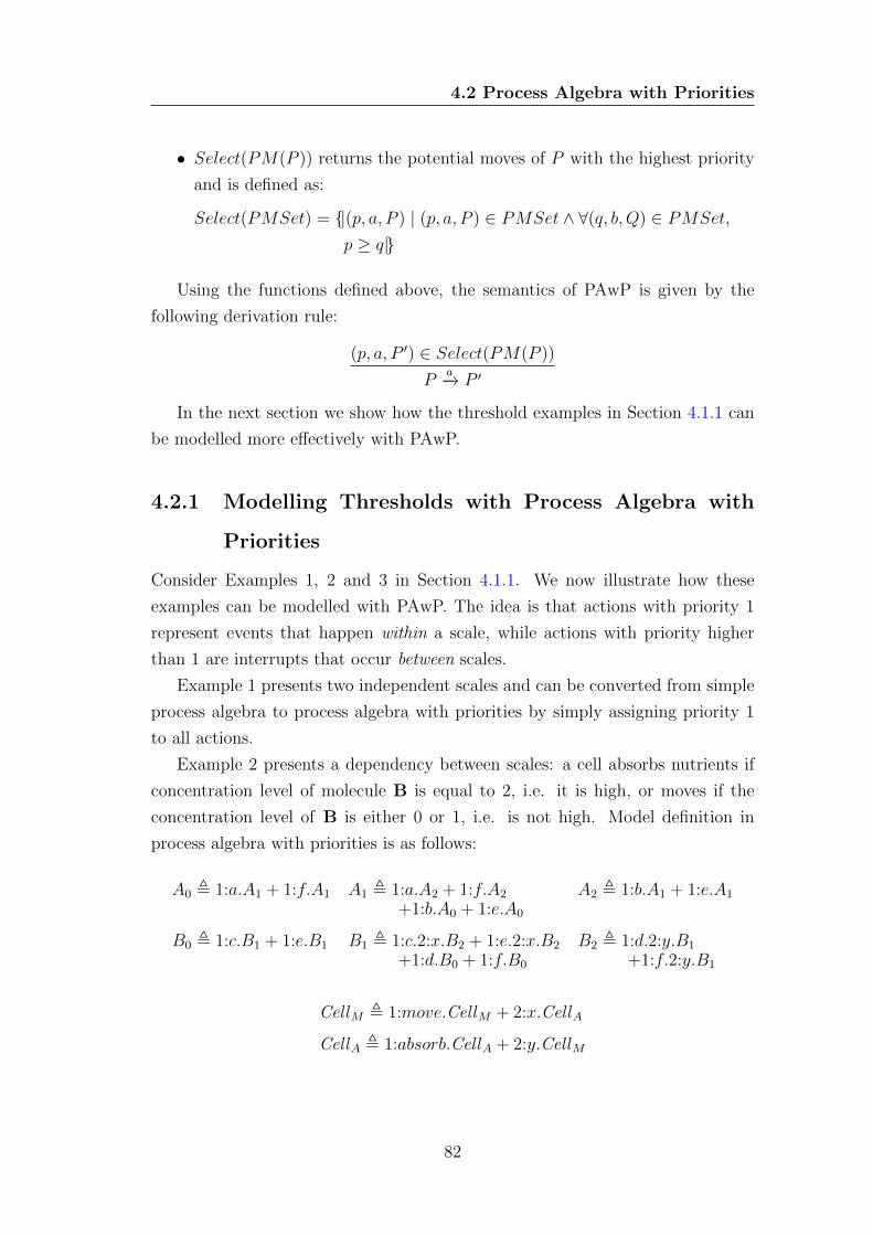
4.2 Process Algebra with Priorities
• Select(PM(P )) returns the potential moves of P with the highest priority
and is defined as:
Select(PMSet) = {|(p, a, P ) | (p, a, P ) ∈ PMSet ∧ ∀(q, b, Q) ∈ PMSet,
p ≥ q|}
Using the functions defined above, the semantics of PAwP is given by the
following derivation rule:
(p, a, P ′) ∈ Select(PM(P ))
Pa−→ P ′
In the next section we show how the threshold examples in Section 4.1.1 can
be modelled more effectively with PAwP.
4.2.1 Modelling Thresholds with Process Algebra with
Priorities
Consider Examples 1, 2 and 3 in Section 4.1.1. We now illustrate how these
examples can be modelled with PAwP. The idea is that actions with priority 1
represent events that happen within a scale, while actions with priority higher
than 1 are interrupts that occur between scales.
Example 1 presents two independent scales and can be converted from simple
process algebra to process algebra with priorities by simply assigning priority 1
to all actions.
Example 2 presents a dependency between scales: a cell absorbs nutrients if
concentration level of molecule B is equal to 2, i.e. it is high, or moves if the
concentration level of B is either 0 or 1, i.e. is not high. Model definition in
process algebra with priorities is as follows:
A0 , 1:a.A1 + 1:f.A1 A1 , 1:a.A2 + 1:f.A2 A2 , 1:b.A1 + 1:e.A1
+1:b.A0 + 1:e.A0
B0 , 1:c.B1 + 1:e.B1 B1 , 1:c.2:x.B2 + 1:e.2:x.B2 B2 , 1:d.2:y.B1
+1:d.B0 + 1:f.B0 +1:f.2:y.B1
CellM , 1:move.CellM + 2:x.CellA
CellA , 1:absorb.CellA + 2:y.CellM
82
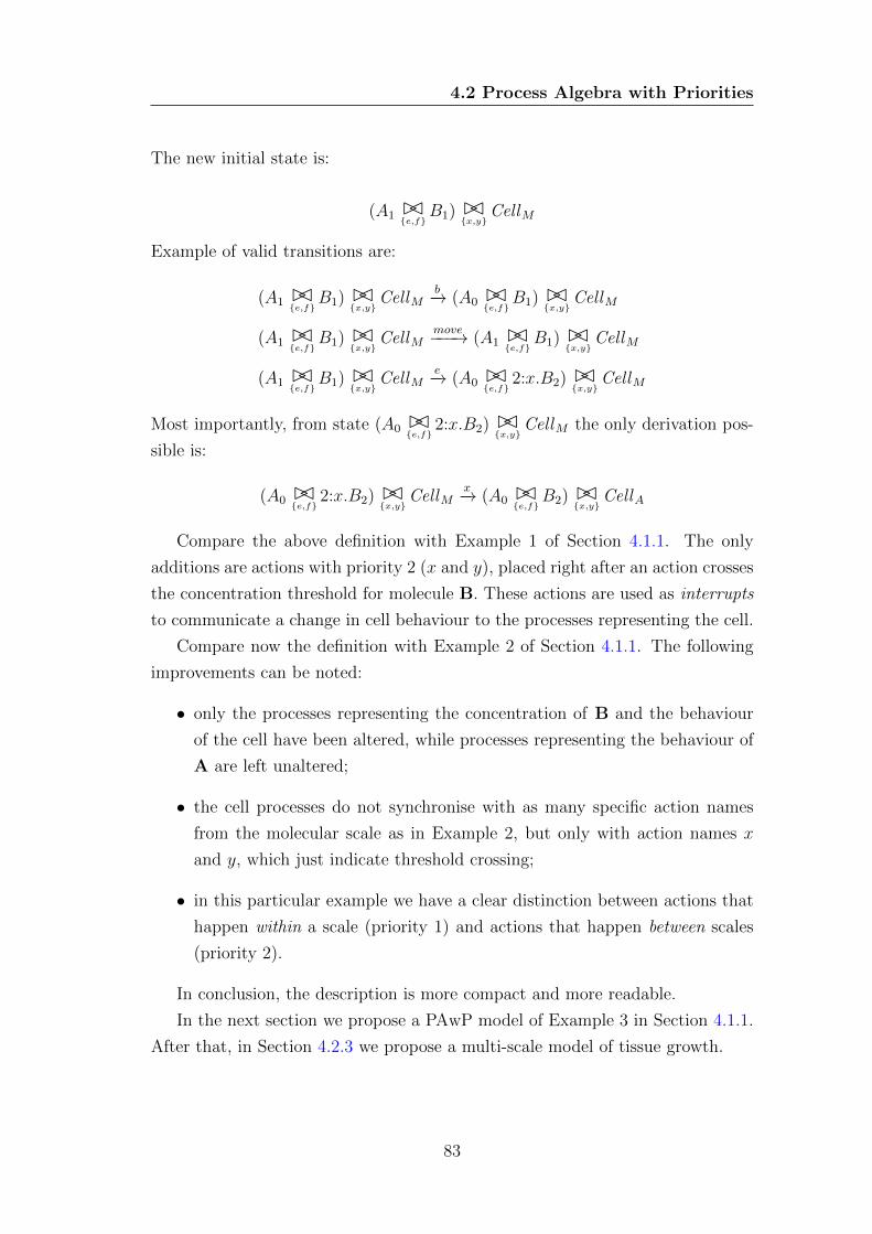
4.2 Process Algebra with Priorities
The new initial state is:
(A1 BC{e,f}B1) BC{x,y}
CellM
Example of valid transitions are:
(A1 BC{e,f}B1) BC{x,y}
CellMb−→ (A0 BC{e,f}B1) BC
{x,y}CellM
(A1 BC{e,f}B1) BC{x,y}
CellMmove−−−→ (A1 BC{e,f}B1) BC
{x,y}CellM
(A1 BC{e,f}B1) BC{x,y}
CellMe−→ (A0 BC{e,f} 2:x.B2) BC
{x,y}CellM
Most importantly, from state (A0 BC{e,f} 2:x.B2) BC{x,y}
CellM the only derivation pos-
sible is:
(A0 BC{e,f} 2:x.B2) BC{x,y}
CellMx−→ (A0 BC{e,f}B2) BC
{x,y}CellA
Compare the above definition with Example 1 of Section 4.1.1. The only
additions are actions with priority 2 (x and y), placed right after an action crosses
the concentration threshold for molecule B. These actions are used as interrupts
to communicate a change in cell behaviour to the processes representing the cell.
Compare now the definition with Example 2 of Section 4.1.1. The following
improvements can be noted:
• only the processes representing the concentration of B and the behaviour
of the cell have been altered, while processes representing the behaviour of
A are left unaltered;
• the cell processes do not synchronise with as many specific action names
from the molecular scale as in Example 2, but only with action names x
and y, which just indicate threshold crossing;
• in this particular example we have a clear distinction between actions that
happen within a scale (priority 1) and actions that happen between scales
(priority 2).
In conclusion, the description is more compact and more readable.
In the next section we propose a PAwP model of Example 3 in Section 4.1.1.
After that, in Section 4.2.3 we propose a multi-scale model of tissue growth.
83
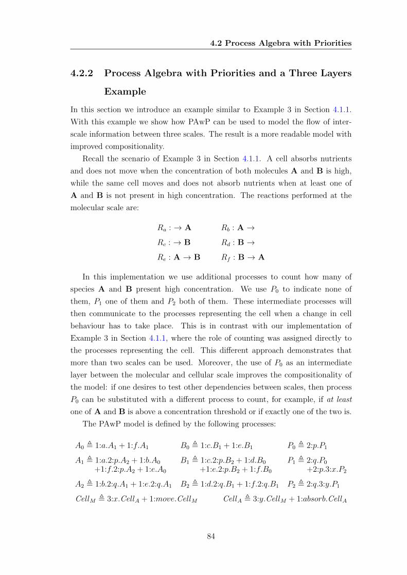
4.2 Process Algebra with Priorities
4.2.2 Process Algebra with Priorities and a Three Layers
Example
In this section we introduce an example similar to Example 3 in Section 4.1.1.
With this example we show how PAwP can be used to model the flow of inter-
scale information between three scales. The result is a more readable model with
improved compositionality.
Recall the scenario of Example 3 in Section 4.1.1. A cell absorbs nutrients
and does not move when the concentration of both molecules A and B is high,
while the same cell moves and does not absorb nutrients when at least one of
A and B is not present in high concentration. The reactions performed at the
molecular scale are:
Ra : → A Rb : A →
Rc : → B Rd : B →
Re : A → B Rf : B → A
In this implementation we use additional processes to count how many of
species A and B present high concentration. We use P0 to indicate none of
them, P1 one of them and P2 both of them. These intermediate processes will
then communicate to the processes representing the cell when a change in cell
behaviour has to take place. This is in contrast with our implementation of
Example 3 in Section 4.1.1, where the role of counting was assigned directly to
the processes representing the cell. This different approach demonstrates that
more than two scales can be used. Moreover, the use of P0 as an intermediate
layer between the molecular and cellular scale improves the compositionality of
the model: if one desires to test other dependencies between scales, then process
P0 can be substituted with a different process to count, for example, if at least
one of A and B is above a concentration threshold or if exactly one of the two is.
The PAwP model is defined by the following processes:
A0 , 1:a.A1 + 1:f.A1 B0 , 1:c.B1 + 1:e.B1 P0 , 2:p.P1
A1 , 1:a.2:p.A2 + 1:b.A0 B1 , 1:c.2:p.B2 + 1:d.B0 P1 , 2:q.P0
+1:f.2:p.A2 + 1:e.A0 +1:e.2:p.B2 + 1:f.B0 +2:p.3:x.P2
A2 , 1:b.2:q.A1 + 1:e.2:q.A1 B2 , 1:d.2:q.B1 + 1:f.2:q.B1 P2 , 2:q.3:y.P1
CellM , 3:x.CellA + 1:move.CellM CellA , 3:y.CellM + 1:absorb.CellA
84
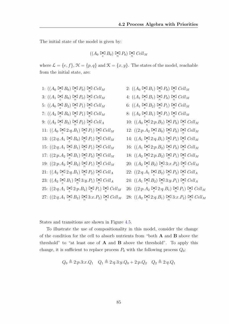
4.2 Process Algebra with Priorities
The initial state of the model is given by:
((A0 BCLB0)BC
HP0)BC
KCellM
where L = {e, f}, H = {p, q} and K = {x, y}. The states of the model, reachable
from the initial state, are:
1: ((A0 BCLB0)BC
HP0)BC
KCellM 2: ((A0 BC
LB1)BC
HP0)BC
KCellM
3: ((A1 BCLB0)BC
HP0)BC
KCellM 4: ((A1 BC
LB1)BC
HP0)BC
KCellM
5: ((A0 BCLB2)BC
HP1)BC
KCellM 6: ((A1 BC
LB2)BC
HP1)BC
KCellM
7: ((A2 BCLB0)BC
HP1)BC
KCellM 8: ((A2 BC
LB1)BC
HP1)BC
KCellM
9: ((A2 BCLB2)BC
HP2)BC
KCellA 10: ((A0 BC
L2:p.B2)BC
HP0)BC
KCellM
11: ((A0 BCL
2:q.B1)BCHP1)BC
KCellM 12: ((2:p.A2 BC
LB0)BC
HP0)BC
KCellM
13: ((2:q.A1 BCLB0)BC
HP1)BC
KCellM 14: ((A1 BC
L2:q.B1)BC
HP1)BC
KCellM
15: ((2:q.A1 BCLB1)BC
HP1)BC
KCellM 16: ((A1 BC
L2:p.B2)BC
HP0)BC
KCellM
17: ((2:p.A2 BCLB1)BC
HP0)BC
KCellM 18: ((A2 BC
L2:p.B2)BC
HP1)BC
KCellM
19: ((2:p.A2 BCLB2)BC
HP1)BC
KCellM 20: ((A2 BC
LB2)BC
H3:x.P2)BC
KCellM
21: ((A2 BCL
2:q.B1)BCHP2)BC
KCellA 22: ((2:q.A1 BC
LB2)BC
HP2)BC
KCellA
23: ((A2 BCLB1)BC
H3:y.P1)BC
KCellA 24: ((A1 BC
LB2)BC
H3:y.P1)BC
KCellA
25: ((2:q.A1 BCL
2:p.B2)BCHP1)BC
KCellM 26: ((2:p.A2 BC
L2:q.B1)BC
HP1)BC
KCellM
27: ((2:q.A1 BCLB2)BC
H3:x.P2)BC
KCellM 28: ((A2 BC
L2:q.B1)BC
H3:x.P2)BC
KCellM
States and transitions are shown in Figure 4.5.
To illustrate the use of compositionality in this model, consider the change
of the condition for the cell to absorb nutrients from “both A and B above the
threshold” to “at least one of A and B above the threshold”. To apply this
change, it is sufficient to replace process P0 with the following process Q0:
Q0 , 2:p.3:x.Q1 Q1 , 2:q.3:y.Q0 + 2:p.Q2 Q2 , 2:q.Q1
85
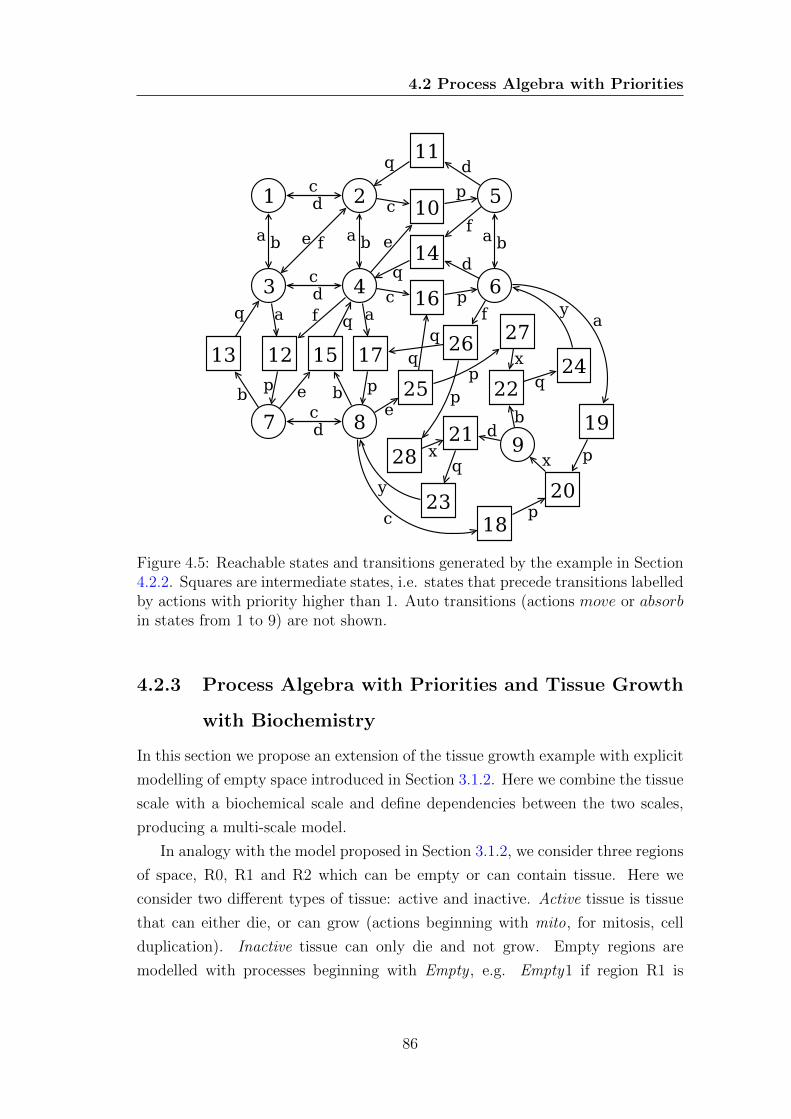
4.2 Process Algebra with Priorities
Figure 4.5: Reachable states and transitions generated by the example in Section4.2.2. Squares are intermediate states, i.e. states that precede transitions labelledby actions with priority higher than 1. Auto transitions (actions move or absorbin states from 1 to 9) are not shown.
4.2.3 Process Algebra with Priorities and Tissue Growth
with Biochemistry
In this section we propose an extension of the tissue growth example with explicit
modelling of empty space introduced in Section 3.1.2. Here we combine the tissue
scale with a biochemical scale and define dependencies between the two scales,
producing a multi-scale model.
In analogy with the model proposed in Section 3.1.2, we consider three regions
of space, R0, R1 and R2 which can be empty or can contain tissue. Here we
consider two different types of tissue: active and inactive. Active tissue is tissue
that can either die, or can grow (actions beginning with mito, for mitosis, cell
duplication). Inactive tissue can only die and not grow. Empty regions are
modelled with processes beginning with Empty , e.g. Empty1 if region R1 is
86
4.2 Process Algebra with Priorities
empty. Active tissue is modelled with processes beginning with Tissueon, e.g.
Tissueon1, that can perform actions beginning with apo, for apoptosis, or actions
beginning with mito, for mitosis, e.g. mito12 if growth happens from region R1
to region R2. Inactive tissue is modelled with processes beginning with Tissueoff ,
e.g. Tissueoff 1, that can perform actions beginning with apo.
The biochemical scale consists of molecular species A, modelled using the pro-
cesses as levels of concentration abstraction, with concentration levels from 0 to
2. Each region contains an independent concentration of A. Processes represent-
ing the concentration of A participate in biochemical reactions, here modelled
with actions a and b, that respectively increment and decrease the concentration
levels of A by one. In addition, we use processes prefixed with NA, that cannot
perform any action, when the corresponding region is empty. For example, we
use NA1 when R1 is empty and no biochemical reactions are possible.
Dependencies between the biochemical and the tissue scale are as follows:
• in a region, tissue is active if and only if the concentration level of A is 2,
while the tissue is inactive otherwise. This dependency is modelled using
the threshold system explained in Section 4.2.1. Actions beginning with
mitoon and mitooff have priority 2 and are used to communicate to the
tissue scale when a threshold has been crossed;
• no biochemical action takes place in empty space. This dependency is
modelled by imposing that whenever a tissue process performs an apoptosis
action, the process representing the concentration of A in the same region
synchronises with that action, changing to an NA process. Analogously,
an NA process changes to a concentration process whenever empty space
turns into tissue.
The model is defined as follows:
87
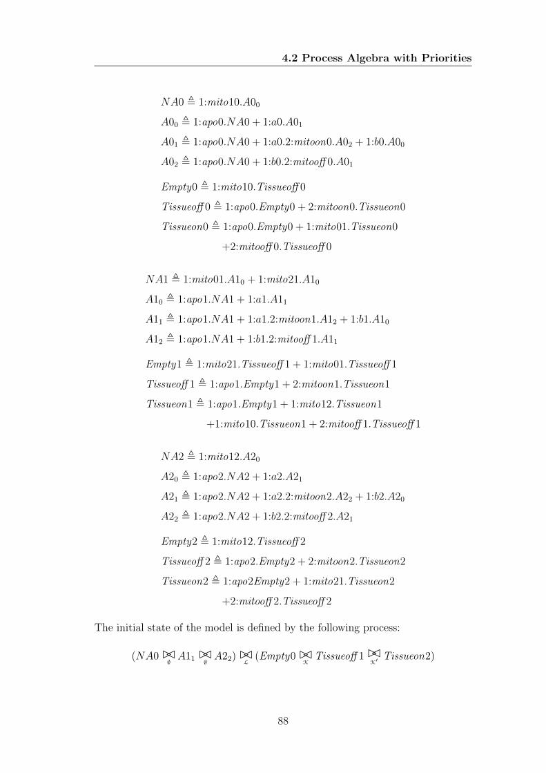
4.2 Process Algebra with Priorities
NA0 , 1:mito10.A00
A00 , 1:apo0.NA0 + 1:a0.A01
A01 , 1:apo0.NA0 + 1:a0.2:mitoon0.A02 + 1:b0.A00
A02 , 1:apo0.NA0 + 1:b0.2:mitooff 0.A01
Empty0 , 1:mito10.Tissueoff 0
Tissueoff 0 , 1:apo0.Empty0 + 2:mitoon0.Tissueon0
Tissueon0 , 1:apo0.Empty0 + 1:mito01.Tissueon0
+2:mitooff 0.Tissueoff 0
NA1 , 1:mito01.A10 + 1:mito21.A10
A10 , 1:apo1.NA1 + 1:a1.A11
A11 , 1:apo1.NA1 + 1:a1.2:mitoon1.A12 + 1:b1.A10
A12 , 1:apo1.NA1 + 1:b1.2:mitooff 1.A11
Empty1 , 1:mito21.Tissueoff 1 + 1:mito01.Tissueoff 1
Tissueoff 1 , 1:apo1.Empty1 + 2:mitoon1.Tissueon1
Tissueon1 , 1:apo1.Empty1 + 1:mito12.Tissueon1
+1:mito10.Tissueon1 + 2:mitooff 1.Tissueoff 1
NA2 , 1:mito12.A20
A20 , 1:apo2.NA2 + 1:a2.A21
A21 , 1:apo2.NA2 + 1:a2.2:mitoon2.A22 + 1:b2.A20
A22 , 1:apo2.NA2 + 1:b2.2:mitooff 2.A21
Empty2 , 1:mito12.Tissueoff 2
Tissueoff 2 , 1:apo2.Empty2 + 2:mitoon2.Tissueon2
Tissueon2 , 1:apo2Empty2 + 1:mito21.Tissueon2
+2:mitooff 2.Tissueoff 2
The initial state of the model is defined by the following process:
(NA0BC∅A11 BC∅ A22)BC
L(Empty0BC
KTissueoff 1BC
K′Tissueon2)
88
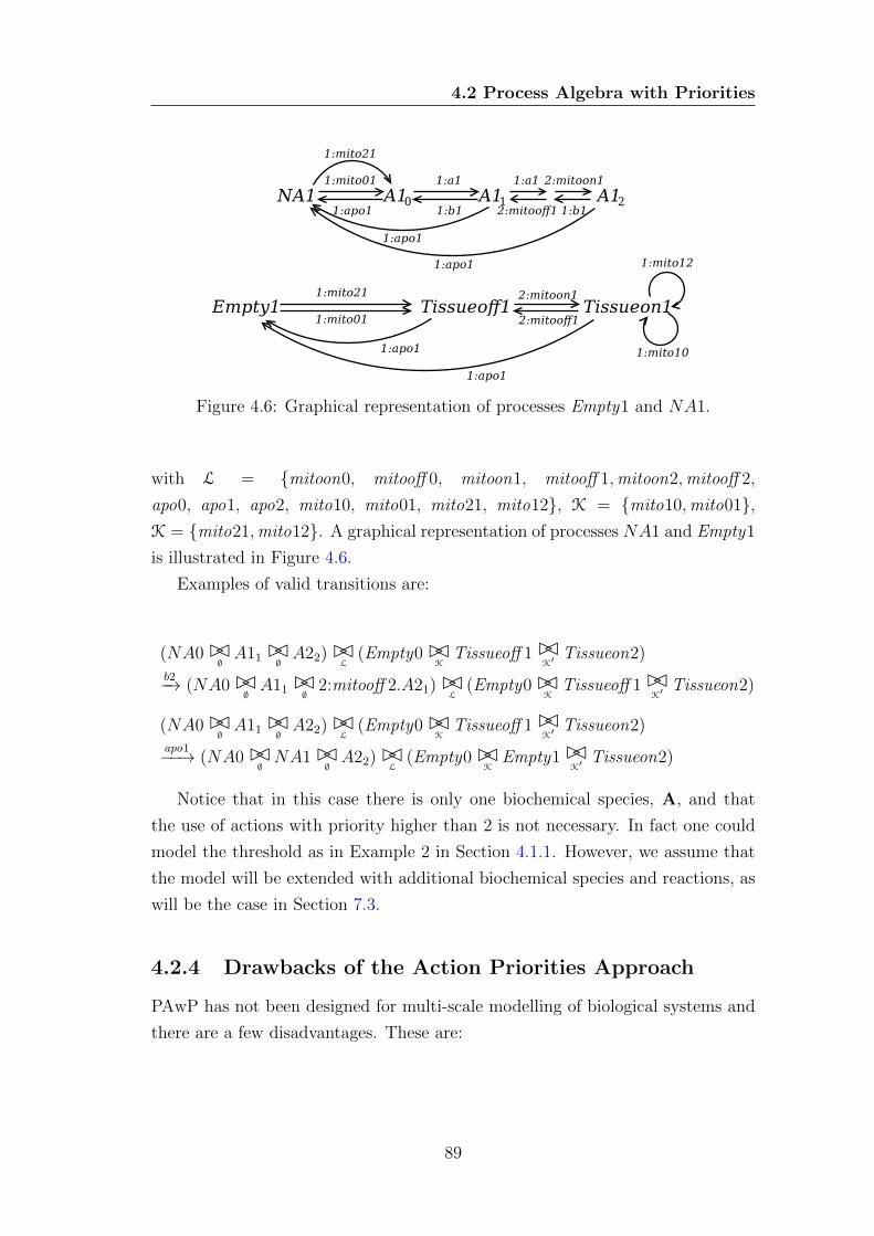
4.2 Process Algebra with Priorities
Figure 4.6: Graphical representation of processes Empty1 and NA1.
with L = {mitoon0, mitooff 0, mitoon1, mitooff 1,mitoon2,mitooff 2,
apo0, apo1, apo2, mito10, mito01, mito21, mito12}, K = {mito10,mito01},K = {mito21,mito12}. A graphical representation of processes NA1 and Empty1
is illustrated in Figure 4.6.
Examples of valid transitions are:
(NA0BC∅A11 BC∅ A22)BC
L(Empty0BC
KTissueoff 1BC
K′Tissueon2)
b2−→ (NA0BC∅A11 BC∅ 2:mitooff 2.A21)BC
L(Empty0BC
KTissueoff 1BC
K′Tissueon2)
(NA0BC∅A11 BC∅ A22)BC
L(Empty0BC
KTissueoff 1BC
K′Tissueon2)
apo1−−→ (NA0BC∅NA1BC
∅A22)BC
L(Empty0BC
KEmpty1BC
K′Tissueon2)
Notice that in this case there is only one biochemical species, A, and that
the use of actions with priority higher than 2 is not necessary. In fact one could
model the threshold as in Example 2 in Section 4.1.1. However, we assume that
the model will be extended with additional biochemical species and reactions, as
will be the case in Section 7.3.
4.2.4 Drawbacks of the Action Priorities Approach
PAwP has not been designed for multi-scale modelling of biological systems and
there are a few disadvantages. These are:
89
4.2 Process Algebra with Priorities
• the introduction of intermediate states, which could be biologically mean-
ingless, i.e. inconsistent with the description of the system modelled. These
states are characterised by outgoing transitions labelled by actions with pri-
ority higher than 1. In Section 4.2.2 states from 10 to 28 are intermediate
states. Some of these states are inconsistent with the definition of the sys-
tem. For example, state 24 present process CellA, representing the food
absorbing phenotype, but only the concentration of B is above a threshold,
instead of both A and B as required. Intermediate states can be removed
in a second moment merging states that are connected by transitions with
action priority higher than 1;
• the use of actions with priorities higher than 1 can produce paths composed
of such actions between two biologically meaningful states. If more than
one path is possible between two states, these paths could contain different
actions. This is a problem if one considers only one of these paths to be
correct. For example, consider the following two paths from Section 4.2.2:
8e−→ 25
p−→ 27x−→ 22
q−→ 24y−→ 6
8e−→ 25
q−→ 16p−→ 6
The two paths between the two biologically meaningful states 8 and 6
present different sequences of actions. In the first path cellular scale ac-
tions x and y are performed, while this is not the case in the second path.
In practice we have a non deterministic choice of behaviour at the cellular
scale. Assume now that in this case only the second sequence of actions
is the correct one. Indeed this is reasonable, because the first sequence
contains x, which should be performed only when both A and B are above
their concentration threshold, while this is not the case because action e
simply converts one level of concentration of A in one of B. The operation
of specifying which path is the correct one will have to be performed a pos-
teriori, once all the paths between two biologically meaningful states have
been computed. We note this operation could be automatic. For example
one could impose that the shortest path is the correct one.
• PAwP does not present syntactic elements that can be used to define explic-
itly and without ambiguities distinct scales and actions that work within
90
4.3 Summary
and between scales. We have discussed in Section 4.2.2 that the compo-
sitionality of a multi-scale model can be improved if actions with priority
1 are used for actions operating within a scale and actions with priority
higher than 1 for actions operating between scales. However, nothing in
the algebra forces a modeller to apply this good practice. For example, in
Section 4.2.3 tissue action apo1 synchronises directly with a biochemical
process such as A11.
The disadvantages mentioned above do not prevent a modeller from using PAwP
in a multi-scale scenario. The first two can be addressed after all transitions from
a state have been computed, while the third is a matter of style of modelling.
4.3 Summary
We began this chapter with a discussion of some of the possible relationships
between spatial scales of biological systems. We then addressed the problem
of modelling such relationships using two existing process algebras with multi-
way synchronisation: simple process algebra and process algebra with priorities.
While the limitations of the first became evident quickly, the second proved to
be fairly well suited to the task. However, process algebra with priorities has
not been designed to model multi-scale scenarios and presents some drawbacks
that have been highlighted at the end of this chapter. Although these drawbacks
do not in general compromise the use of process algebra with priorities, they
nevertheless need to be addressed outside the syntax and the semantics of the
algebra.
In the next chapter we introduce a process algebra with hooks that has been
designed for multi-scale modelling and addresses the above drawbacks. For com-
pleteness, we define a stochastic semantics for process algebra with priorities
based on functional rates, in analogy with Section 3.2.1. This can be found in
Appendix A.
91
Chapter 5
Multi-Scale Modelling with
Process Algebra with Hooks
In this chapter we introduce process algebra with hooks, a process algebra de-
signed for multi-scale modelling of biological systems. In Section 5.1 we introduce
the syntax, the main novel features are composed actions and a new vertical oper-
ator. Together, these features provide explicit modelling of scales and interactions
within and between scales. In Section 5.1.1 we give some basic examples using
process algebra with hooks and in Sections 5.1.2 and 5.1.3 we give process algebra
with hooks versions of the examples introduced in the previous chapter. A com-
parison between process algebra with hooks and process algebra with priorities
is given in Section 5.1.4. Finally, we present a stochastic version of the algebra
based on functional rates in Section 5.2, with additional examples in Sections
5.2.4 and 5.2.3.
5.1 Process Algebra with Hooks
A preliminary version of process algebra with hooks (PAH) has been published
in (Degasperi and Calder, 2010). In our previous work we followed a bottom-up
approach where the biochemical scale determines the rates and other scales are
abstractions of lower scales. Here we follow a middle-out (Noble, 2006) approach
where one can begin modelling at any scale, and then relate to higher or lower
scales.
92
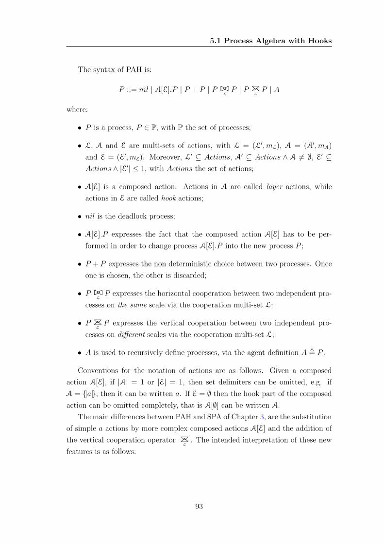
5.1 Process Algebra with Hooks
The syntax of PAH is:
P ::= nil | A[E].P | P + P | P BCLP | P BC
LP | A
where:
• P is a process, P ∈ P, with P the set of processes;
• L, A and E are multi-sets of actions, with L = (L′,mL), A = (A′,mA)
and E = (E′,mE). Moreover, L′ ⊆ Actions, A′ ⊆ Actions ∧ A 6= ∅, E′ ⊆Actions ∧ |E′| ≤ 1, with Actions the set of actions;
• A[E] is a composed action. Actions in A are called layer actions, while
actions in E are called hook actions;
• nil is the deadlock process;
• A[E].P expresses the fact that the composed action A[E] has to be per-
formed in order to change process A[E].P into the new process P ;
• P + P expresses the non deterministic choice between two processes. Once
one is chosen, the other is discarded;
• P BCLP expresses the horizontal cooperation between two independent pro-
cesses on the same scale via the cooperation multi-set L;
• P BC
LP expresses the vertical cooperation between two independent pro-
cesses on different scales via the cooperation multi-set L;
• A is used to recursively define processes, via the agent definition A , P .
Conventions for the notation of actions are as follows. Given a composed
action A[E], if |A| = 1 or |E| = 1, then set delimiters can be omitted, e.g. if
A = {|a|}, then it can be written a. If E = ∅ then the hook part of the composed
action can be omitted completely, that is A[∅] can be written A.
The main differences between PAH and SPA of Chapter 3, are the substitution
of simple a actions by more complex composed actions A[E] and the addition of
the vertical cooperation operator BC
L. The intended interpretation of these new
features is as follows:
93
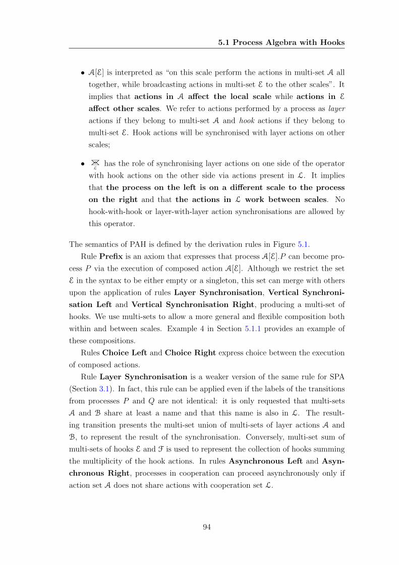
5.1 Process Algebra with Hooks
• A[E] is interpreted as “on this scale perform the actions in multi-set A all
together, while broadcasting actions in multi-set E to the other scales”. It
implies that actions in A affect the local scale while actions in E
affect other scales. We refer to actions performed by a process as layer
actions if they belong to multi-set A and hook actions if they belong to
multi-set E. Hook actions will be synchronised with layer actions on other
scales;
• BC
Lhas the role of synchronising layer actions on one side of the operator
with hook actions on the other side via actions present in L. It implies
that the process on the left is on a different scale to the process
on the right and that the actions in L work between scales. No
hook-with-hook or layer-with-layer action synchronisations are allowed by
this operator.
The semantics of PAH is defined by the derivation rules in Figure 5.1.
Rule Prefix is an axiom that expresses that process A[E].P can become pro-
cess P via the execution of composed action A[E]. Although we restrict the set
E in the syntax to be either empty or a singleton, this set can merge with others
upon the application of rules Layer Synchronisation, Vertical Synchroni-
sation Left and Vertical Synchronisation Right, producing a multi-set of
hooks. We use multi-sets to allow a more general and flexible composition both
within and between scales. Example 4 in Section 5.1.1 provides an example of
these compositions.
Rules Choice Left and Choice Right express choice between the execution
of composed actions.
Rule Layer Synchronisation is a weaker version of the same rule for SPA
(Section 3.1). In fact, this rule can be applied even if the labels of the transitions
from processes P and Q are not identical: it is only requested that multi-sets
A and B share at least a name and that this name is also in L. The result-
ing transition presents the multi-set union of multi-sets of layer actions A and
B, to represent the result of the synchronisation. Conversely, multi-set sum of
multi-sets of hooks E and F is used to represent the collection of hooks summing
the multiplicity of the hook actions. In rules Asynchronous Left and Asyn-
chronous Right, processes in cooperation can proceed asynchronously only if
action set A does not share actions with cooperation set L.
94
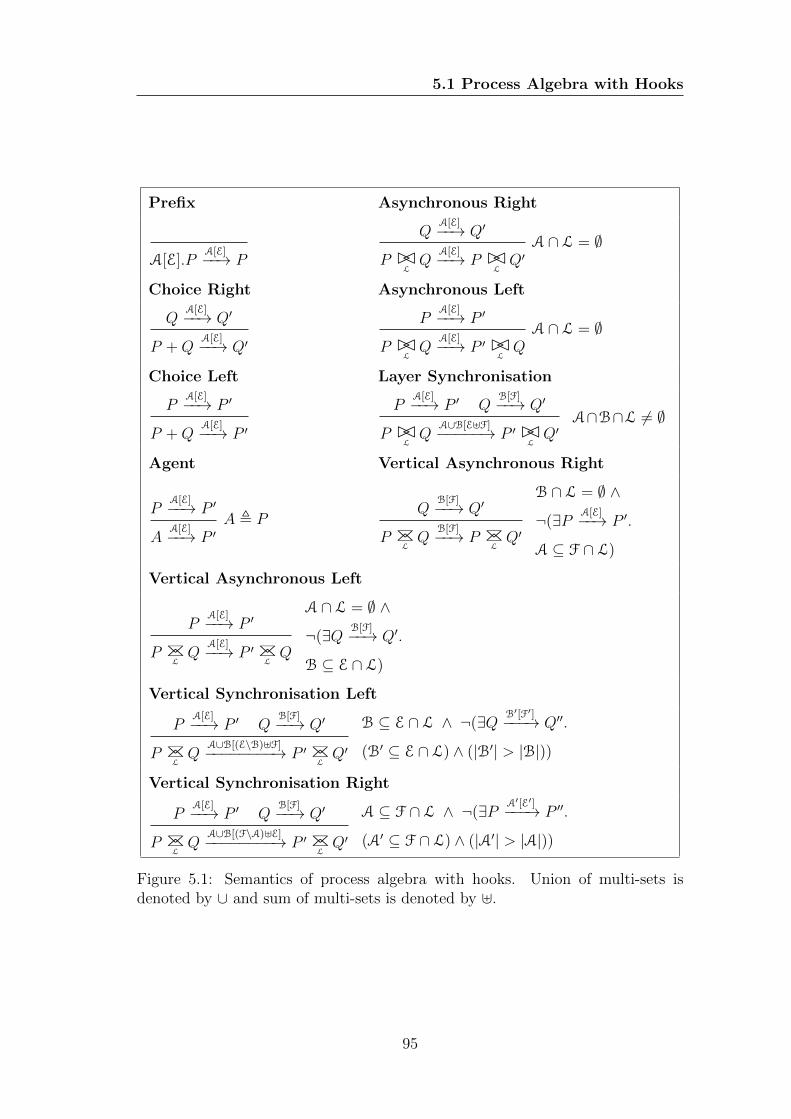
5.1 Process Algebra with Hooks
Prefix Asynchronous Right
A[E].PA[E]−−→ P
QA[E]−−→ Q′
P BCLQ
A[E]−−→ P BCLQ′
A ∩ L = ∅
Choice Right Asynchronous Left
QA[E]−−→ Q′
P +QA[E]−−→ Q′
PA[E]−−→ P ′
P BCLQ
A[E]−−→ P ′ BCLQ
A ∩ L = ∅
Choice Left Layer Synchronisation
PA[E]−−→ P ′
P +QA[E]−−→ P ′
PA[E]−−→ P ′ Q
B[F]−−→ Q′
P BCLQ
A∪B[E]F]−−−−−→ P ′ BCLQ′
A∩B∩L 6= ∅
Agent Vertical Asynchronous Right
PA[E]−−→ P ′
AA[E]−−→ P ′
A , PQ
B[F]−−→ Q′
P BC
LQ
B[F]−−→ P BC
LQ′
B ∩ L = ∅ ∧
¬(∃P A[E]−−→ P ′.
A ⊆ F ∩ L)
Vertical Asynchronous Left
PA[E]−−→ P ′
P BC
LQ
A[E]−−→ P ′ BC
LQ
A ∩ L = ∅ ∧
¬(∃Q B[F]−−→ Q′.
B ⊆ E ∩ L)
Vertical Synchronisation Left
PA[E]−−→ P ′ Q
B[F]−−→ Q′
P BC
LQ
A∪B[(E\B)]F]−−−−−−−−→ P ′ BC
LQ′
B ⊆ E ∩ L ∧ ¬(∃Q B′[F′]−−−→ Q′′.
(B′ ⊆ E ∩ L) ∧ (|B′| > |B|))
Vertical Synchronisation Right
PA[E]−−→ P ′ Q
B[F]−−→ Q′
P BC
LQ
A∪B[(F\A)]E]−−−−−−−−→ P ′ BC
LQ′
A ⊆ F ∩ L ∧ ¬(∃P A′[E′]−−−→ P ′′.
(A′ ⊆ F ∩ L) ∧ (|A′| > |A|))
Figure 5.1: Semantics of process algebra with hooks. Union of multi-sets isdenoted by ∪ and sum of multi-sets is denoted by ].
95
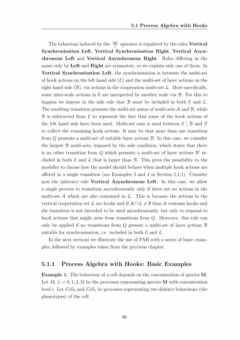
5.1 Process Algebra with Hooks
The behaviour induced by the BC
Loperator is regulated by the rules Vertical
Synchronisation Left, Vertical Synchronisation Right, Vertical Asyn-
chronous Left and Vertical Asynchronous Right. Rules differing in the
name only by Left and Right are symmetric, so we explain only one of them. In
Vertical Synchronisation Left, the synchronisation is between the multi-set
of hook actions on the left hand side (E) and the multi-set of layer actions on the
right hand side (B), via actions in the cooperation multi-set L. More specifically,
some inter-scale actions in E are interpreted by another scale via B. For this to
happen we impose in the side rule that B must be included in both E and L.
The resulting transition presents the multi-set union of multi-sets A and B, while
B is subtracted from E to represent the fact that some of the hook actions of
the left hand side have been used. Multi-set sum is used between E \ B and F
to collect the remaining hook actions. It may be that more than one transition
from Q presents a multi-set of suitable layer actions B. In this case, we consider
the largest B multi-sets, imposed by the side condition, which states that there
is no other transition from Q which presents a multi-set of layer actions B′ in-
cluded in both E and L that is larger than B. This gives the possibility to the
modeller to choose how the model should behave when multiple hook actions are
offered in a single transition (see Examples 3 and 4 in Section 5.1.1). Consider
now the inference rule Vertical Asynchronous Left. In this case, we allow
a single process to transition asynchronously only if there are no actions in the
multi-set A which are also contained in L. This is because the actions in the
vertical cooperation set L are hooks and if A∩L 6= ∅ then A contains hooks and
the transition is not intended to be used asynchronously, but only to respond to
hook actions that might arise from transitions from Q. Moreover, this rule can
only be applied if no transitions from Q present a multi-set of layer actions B
suitable for synchronisation, i.e. included in both E and L.
In the next sections we illustrate the use of PAH with a series of basic exam-
ples, followed by examples taken from the previous chapter.
5.1.1 Process Algebra with Hooks: Basic Examples
Example 1. The behaviour of a cell depends on the concentration of species M.
Let Mi (i = 0, 1, 2, 3) be the processes representing species M with concentration
level i. Let Cell0 and Cell1 be processes representing two distinct behaviours (the
phenotypes) of the cell.
96
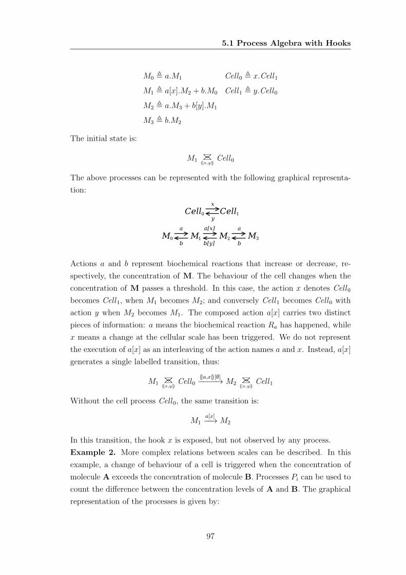
5.1 Process Algebra with Hooks
M0 , a.M1 Cell0 , x.Cell1
M1 , a[x].M2 + b.M0 Cell1 , y.Cell0
M2 , a.M3 + b[y].M1
M3 , b.M2
The initial state is:
M1 BC
{|x,y|}Cell0
The above processes can be represented with the following graphical representa-
tion:
Actions a and b represent biochemical reactions that increase or decrease, re-
spectively, the concentration of M. The behaviour of the cell changes when the
concentration of M passes a threshold. In this case, the action x denotes Cell0
becomes Cell1, when M1 becomes M2; and conversely Cell1 becomes Cell0 with
action y when M2 becomes M1. The composed action a[x] carries two distinct
pieces of information: a means the biochemical reaction Ra has happened, while
x means a change at the cellular scale has been triggered. We do not represent
the execution of a[x] as an interleaving of the action names a and x. Instead, a[x]
generates a single labelled transition, thus:
M1 BC
{|x,y|}Cell0
{|a,x|}[∅]−−−−→M2 BC
{|x,y|}Cell1
Without the cell process Cell0, the same transition is:
M1a[x]−−→M2
In this transition, the hook x is exposed, but not observed by any process.
Example 2. More complex relations between scales can be described. In this
example, a change of behaviour of a cell is triggered when the concentration of
molecule A exceeds the concentration of molecule B. Processes Pi can be used to
count the difference between the concentration levels of A and B. The graphical
representation of the processes is given by:
97
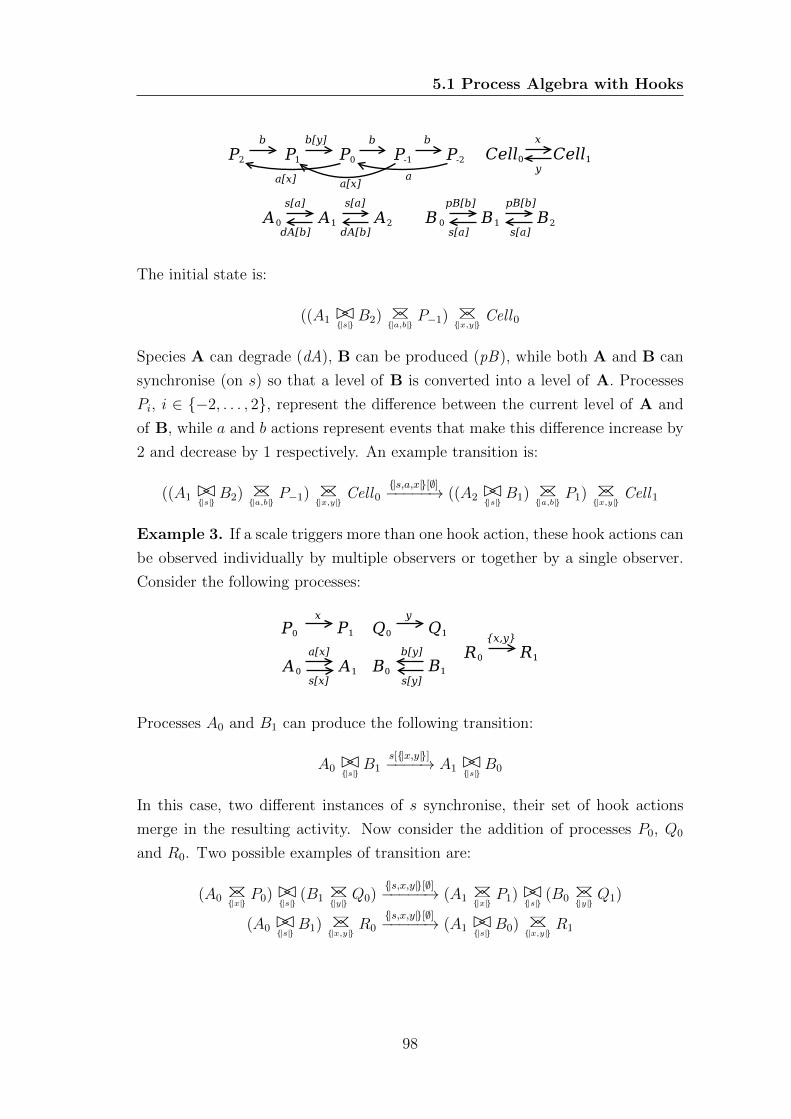
5.1 Process Algebra with Hooks
The initial state is:
((A1 BC{|s|} B2) BC
{|a,b|}P−1) BC
{|x,y|}Cell0
Species A can degrade (dA), B can be produced (pB), while both A and B can
synchronise (on s) so that a level of B is converted into a level of A. Processes
Pi, i ∈ {−2, . . . , 2}, represent the difference between the current level of A and
of B, while a and b actions represent events that make this difference increase by
2 and decrease by 1 respectively. An example transition is:
((A1 BC{|s|} B2) BC
{|a,b|}P−1) BC
{|x,y|}Cell0
{|s,a,x|}[∅]−−−−−→ ((A2 BC{|s|} B1) BC
{|a,b|}P1) BC
{|x,y|}Cell1
Example 3. If a scale triggers more than one hook action, these hook actions can
be observed individually by multiple observers or together by a single observer.
Consider the following processes:
Processes A0 and B1 can produce the following transition:
A0 BC{|s|} B1s[{|x,y|}]−−−−→ A1 BC{|s|} B0
In this case, two different instances of s synchronise, their set of hook actions
merge in the resulting activity. Now consider the addition of processes P0, Q0
and R0. Two possible examples of transition are:
(A0 BC
{|x|}P0)BC
{|s|}(B1 BC
{|y|}Q0)
{|s,x,y|}[∅]−−−−−→ (A1 BC
{|x|}P1)BC
{|s|}(B0 BC
{|y|}Q1)
(A0 BC{|s|} B1) BC
{|x,y|}R0
{|s,x,y|}[∅]−−−−−→ (A1 BC{|s|} B0) BC
{|x,y|}R1
98
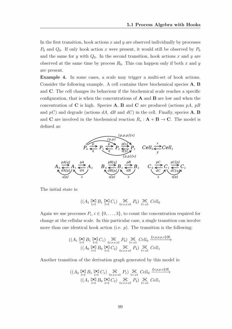
5.1 Process Algebra with Hooks
In the first transition, hook actions x and y are observed individually by processes
P0 and Q0. If only hook action x were present, it would still be observed by P0
and the same for y with Q0. In the second transition, hook actions x and y are
observed at the same time by process R0. This can happen only if both x and y
are present.
Example 4. In some cases, a scale may trigger a multi-set of hook actions.
Consider the following example. A cell contains three biochemical species A, B
and C. The cell changes its behaviour if the biochemical scale reaches a specific
configuration, that is when the concentrations of A and B are low and when the
concentration of C is high. Species A, B and C are produced (actions pA, pB
and pC ) and degrade (actions dA, dB and dC ) in the cell. Finally, species A, B
and C are involved in the biochemical reaction Rs : A + B → C. The model is
defined as:
The initial state is:
((A1 BC{|s|} B1 BC{|s|} C1) BC
{|p,p,p,q|}P0) BC
{|x,y|}Cell0
Again we use processes Pi, i ∈ {0, . . . , 3}, to count the concentration required for
change at the cellular scale. In this particular case, a single transition can involve
more than one identical hook action (i.e. p). The transition is the following:
((A1 BC{|s|} B1 BC{|s|} C1) BC
{|p,p,p,q|}P0) BC
{|x,y|}Cell0
{|s,p,p,p,x|}[∅]−−−−−−−→
((A0 BC{|s|} B0 BC{|s|} C2) BC
{|p,p,p,q|}P3) BC
{|x,y|}Cell1
Another transition of the derivation graph generated by this model is:
((A2 BC{|s|} B1 BC{|s|} C1) BC
{|p,p,p,q|}P1) BC
{|x,y|}Cell0
{|s,p,p,x|}[∅]−−−−−−→
((A1 BC{|s|} B0 BC{|s|} C2) BC
{|p,p,p,q|}P3) BC
{|x,y|}Cell1
99
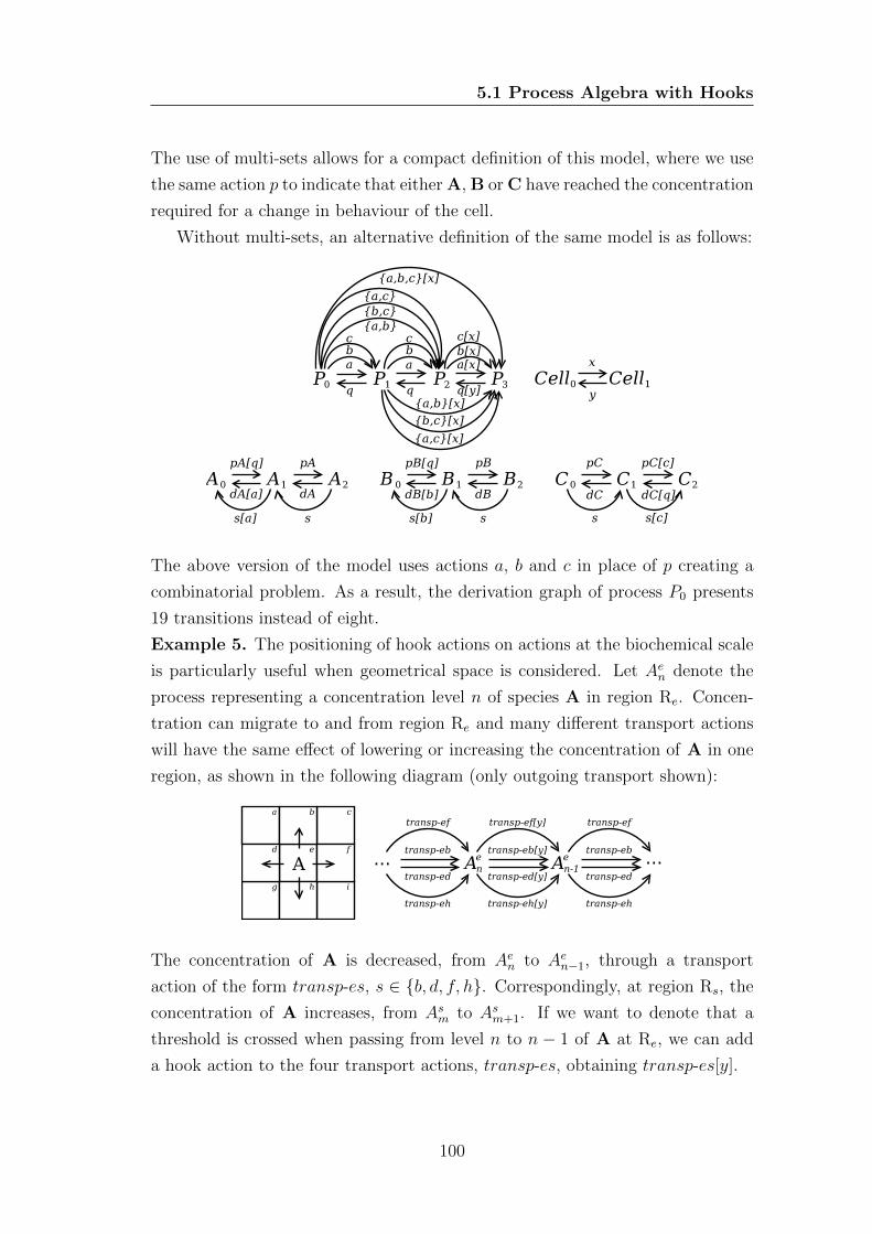
5.1 Process Algebra with Hooks
The use of multi-sets allows for a compact definition of this model, where we use
the same action p to indicate that either A, B or C have reached the concentration
required for a change in behaviour of the cell.
Without multi-sets, an alternative definition of the same model is as follows:
The above version of the model uses actions a, b and c in place of p creating a
combinatorial problem. As a result, the derivation graph of process P0 presents
19 transitions instead of eight.
Example 5. The positioning of hook actions on actions at the biochemical scale
is particularly useful when geometrical space is considered. Let Aen denote the
process representing a concentration level n of species A in region Re. Concen-
tration can migrate to and from region Re and many different transport actions
will have the same effect of lowering or increasing the concentration of A in one
region, as shown in the following diagram (only outgoing transport shown):
The concentration of A is decreased, from Aen to Aen−1, through a transport
action of the form transp-es, s ∈ {b, d, f, h}. Correspondingly, at region Rs, the
concentration of A increases, from Asm to Asm+1. If we want to denote that a
threshold is crossed when passing from level n to n − 1 of A at Re, we can add
a hook action to the four transport actions, transp-es, obtaining transp-es[y].
100
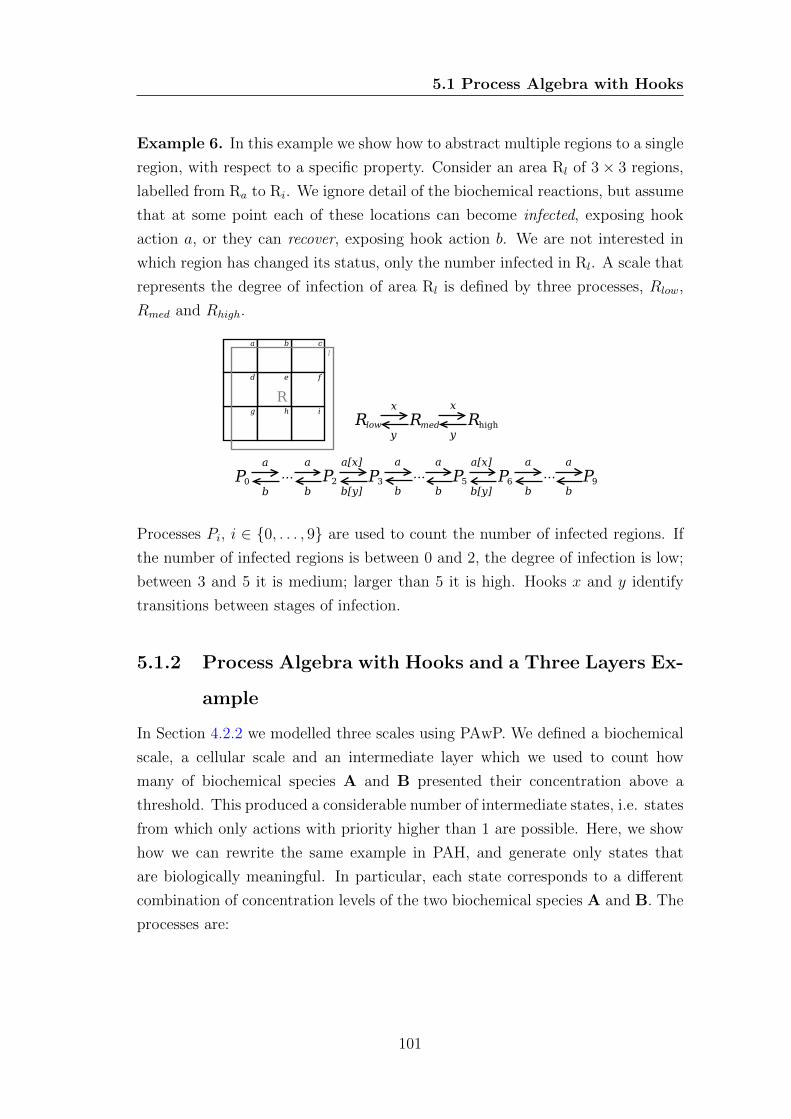
5.1 Process Algebra with Hooks
Example 6. In this example we show how to abstract multiple regions to a single
region, with respect to a specific property. Consider an area Rl of 3× 3 regions,
labelled from Ra to Ri. We ignore detail of the biochemical reactions, but assume
that at some point each of these locations can become infected, exposing hook
action a, or they can recover, exposing hook action b. We are not interested in
which region has changed its status, only the number infected in Rl. A scale that
represents the degree of infection of area Rl is defined by three processes, Rlow,
Rmed and Rhigh.
Processes Pi, i ∈ {0, . . . , 9} are used to count the number of infected regions. If
the number of infected regions is between 0 and 2, the degree of infection is low;
between 3 and 5 it is medium; larger than 5 it is high. Hooks x and y identify
transitions between stages of infection.
5.1.2 Process Algebra with Hooks and a Three Layers Ex-
ample
In Section 4.2.2 we modelled three scales using PAwP. We defined a biochemical
scale, a cellular scale and an intermediate layer which we used to count how
many of biochemical species A and B presented their concentration above a
threshold. This produced a considerable number of intermediate states, i.e. states
from which only actions with priority higher than 1 are possible. Here, we show
how we can rewrite the same example in PAH, and generate only states that
are biologically meaningful. In particular, each state corresponds to a different
combination of concentration levels of the two biochemical species A and B. The
processes are:
101
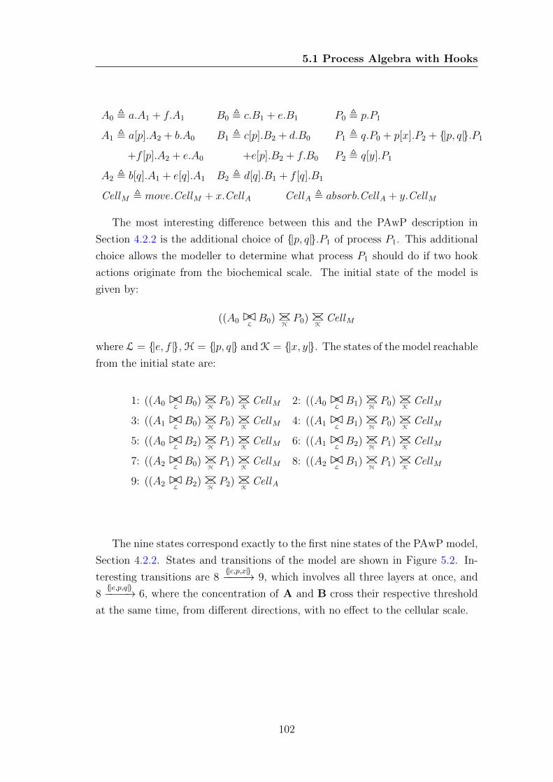
5.1 Process Algebra with Hooks
A0 , a.A1 + f.A1 B0 , c.B1 + e.B1 P0 , p.P1
A1 , a[p].A2 + b.A0 B1 , c[p].B2 + d.B0 P1 , q.P0 + p[x].P2 + {|p, q|}.P1
+f [p].A2 + e.A0 +e[p].B2 + f.B0 P2 , q[y].P1
A2 , b[q].A1 + e[q].A1 B2 , d[q].B1 + f [q].B1
CellM , move.CellM + x.CellA CellA , absorb.CellA + y.CellM
The most interesting difference between this and the PAwP description in
Section 4.2.2 is the additional choice of {|p, q|}.P1 of process P1. This additional
choice allows the modeller to determine what process P1 should do if two hook
actions originate from the biochemical scale. The initial state of the model is
given by:
((A0 BCLB0) BC
HP0) BC
KCellM
where L = {|e, f |}, H = {|p, q|} and K = {|x, y|}. The states of the model reachable
from the initial state are:
1: ((A0 BCLB0) BC
HP0) BC
KCellM 2: ((A0 BC
LB1) BC
HP0) BC
KCellM
3: ((A1 BCLB0) BC
HP0) BC
KCellM 4: ((A1 BC
LB1) BC
HP0) BC
KCellM
5: ((A0 BCLB2) BC
HP1) BC
KCellM 6: ((A1 BC
LB2) BC
HP1) BC
KCellM
7: ((A2 BCLB0) BC
HP1) BC
KCellM 8: ((A2 BC
LB1) BC
HP1) BC
KCellM
9: ((A2 BCLB2) BC
HP2) BC
KCellA
The nine states correspond exactly to the first nine states of the PAwP model,
Section 4.2.2. States and transitions of the model are shown in Figure 5.2. In-
teresting transitions are 8{|c,p,x|}−−−−→ 9, which involves all three layers at once, and
8{|e,p,q|}−−−−→ 6, where the concentration of A and B cross their respective threshold
at the same time, from different directions, with no effect to the cellular scale.
102
5.1 Process Algebra with Hooks
Figure 5.2: Reachable states and transitions generated by the example in Section5.1.2.
5.1.3 Process Algebra with Hooks and Tissue Growth with
Biochemistry
In this section we show how the example introduced in Section 4.2.3 can be
modelled using PAH. Because PAH adopts an explicit distinction between actions
operating within a scale and between scales, new actions have to be introduced.
In particular, a direct synchronisation between biochemical and tissue scales via
actions such as apo1 or mito21 would be prevented by the vertical operator BCL
.
Instead, we introduce inter-scale actions bioff 1 and bioon1 to communicate the
effects of apo1 and mito21 across scales. Processes can be rewritten as follows:
NA0 , bioon0.A00
A00 , biooff 0.NA0 + a0.A01
A01 , biooff 0.NA0 + a0[mitoon0].A02 + b0.A00
A02 , biooff 0.NA0 + b0[mitooff 0].A01
Empty0 , mito10[bioon0].Tissueoff 0
Tissueoff 0 , apo0[biooff 0].Empty0 + mitoon0.Tissueon0
Tissueon0 , apo0[biooff 0].Empty0 + [mito01].Tissueon0
+mitooff 0.Tissueoff 0
103
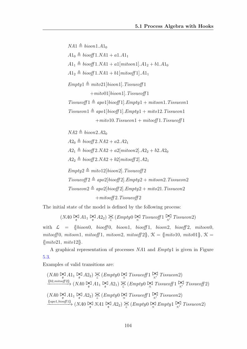
5.1 Process Algebra with Hooks
NA1 , bioon1.A10
A10 , biooff 1.NA1 + a1.A11
A11 , biooff 1.NA1 + a1[mitoon1].A12 + b1.A10
A12 , biooff 1.NA1 + b1[mitooff 1].A11
Empty1 , mito21[bioon1].Tissueoff 1
+mito01[bioon1].Tissueoff 1
Tissueoff 1 , apo1[biooff 1].Empty1 + mitoon1.Tissueon1
Tissueon1 , apo1[biooff 1].Empty1 + mito12.Tissueon1
+mito10.Tissueon1 + mitooff 1.Tissueoff 1
NA2 , bioon2.A20
A20 , biooff 2.NA2 + a2.A21
A21 , biooff 2.NA2 + a2[mitoon2].A22 + b2.A20
A22 , biooff 2.NA2 + b2[mitooff 2].A21
Empty2 , mito12[bioon2].Tissueoff 2
Tissueoff 2 , apo2[biooff 2].Empty2 + mitoon2.Tissueon2
Tissueon2 , apo2[biooff 2].Empty2 + mito21.Tissueon2
+mitooff 2.Tissueoff 2
The initial state of the model is defined by the following process:
(NA0BC∅A11 BC∅ A22) BC
L(Empty0BC
KTissueoff 1BC
K′Tissueon2)
with L = {|bioon0, biooff 0, bioon1, biooff 1, bioon2, biooff 2, mitoon0,
mitooff 0, mitoon1, mitooff 1, mitoon2, mitooff 2|}, K = {|mito10, mito01|}, K =
{|mito21, mito12|}.A graphical representation of processes NA1 and Empty1 is given in Figure
5.3.
Examples of valid transitions are:
(NA0BC∅A11 BC∅ A22) BC
L(Empty0BC
KTissueoff 1BC
K′Tissueon2)
{|b2,mitooff 2|}−−−−−−−−→ (NA0BC∅A11 BC∅ A21) BC
L(Empty0BC
KTissueoff 1BC
K′Tissueoff 2)
(NA0BC∅A11 BC∅ A22) BC
L(Empty0BC
KTissueoff 1BC
K′Tissueon2)
{|apo1,biooff 1|}−−−−−−−−→ (NA0BC∅
NA1BC∅A22) BC
L(Empty0BC
KEmpty1BC
K′Tissueon2)
104
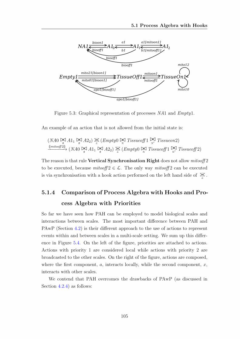
5.1 Process Algebra with Hooks
Figure 5.3: Graphical representation of processes NA1 and Empty1.
An example of an action that is not allowed from the initial state is:
(NA0BC∅A11 BC∅ A22) BC
L(Empty0BC
KTissueoff 1BC
K′Tissueon2)
{|mitooff 2|}−−−−−−→ (NA0BC∅A11 BC∅ A22) BC
L(Empty0BC
KTissueoff 1BC
K′Tissueoff 2)
The reason is that rule Vertical Synchronisation Right does not allow mitooff 2
to be executed, because mitooff 2 ∈ L. The only way mitooff 2 can be executed
is via synchronisation with a hook action performed on the left hand side of BC
L.
5.1.4 Comparison of Process Algebra with Hooks and Pro-
cess Algebra with Priorities
So far we have seen how PAH can be employed to model biological scales and
interactions between scales. The most important difference between PAH and
PAwP (Section 4.2) is their different approach to the use of actions to represent
events within and between scales in a multi-scale setting. We sum up this differ-
ence in Figure 5.4. On the left of the figure, priorities are attached to actions.
Actions with priority 1 are considered local while actions with priority 2 are
broadcasted to the other scales. On the right of the figure, actions are composed,
where the first component, a, interacts locally, while the second component, x,
interacts with other scales.
We contend that PAH overcomes the drawbacks of PAwP (as discussed in
Section 4.2.4) as follows:
105
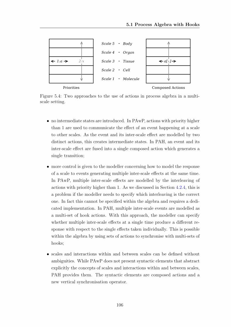
5.1 Process Algebra with Hooks
Figure 5.4: Two approaches to the use of actions in process algebra in a multi-scale setting.
• no intermediate states are introduced. In PAwP, actions with priority higher
than 1 are used to communicate the effect of an event happening at a scale
to other scales. As the event and its inter-scale effect are modelled by two
distinct actions, this creates intermediate states. In PAH, an event and its
inter-scale effect are fused into a single composed action which generates a
single transition;
• more control is given to the modeller concerning how to model the response
of a scale to events generating multiple inter-scale effects at the same time.
In PAwP, multiple inter-scale effects are modelled by the interleaving of
actions with priority higher than 1. As we discussed in Section 4.2.4, this is
a problem if the modeller needs to specify which interleaving is the correct
one. In fact this cannot be specified within the algebra and requires a dedi-
cated implementation. In PAH, multiple inter-scale events are modelled as
a multi-set of hook actions. With this approach, the modeller can specify
whether multiple inter-scale effects at a single time produce a different re-
sponse with respect to the single effects taken individually. This is possible
within the algebra by using sets of actions to synchronise with multi-sets of
hooks;
• scales and interactions within and between scales can be defined without
ambiguities. While PAwP does not present syntactic elements that abstract
explicitly the concepts of scales and interactions within and between scales,
PAH provides them. The syntactic elements are composed actions and a
new vertical synchronisation operator.
106
5.2 Stochastic Semantics for Process Algebra with Hooks
In the next section we introduce a stochastic semantics for PAH.
5.2 Stochastic Semantics for Process Algebra with
Hooks
In this section we define a stochastic semantics for PAH, in analogy with Section
3.2.1. Before we give a formal definition, we illustrate the main challenges with
an example.
Consider Example 2 of Section 4.1.1. In PAH agent definitions are as follows:
A0 , a.A1 + f.A1 A1 , a.A2 + f.A2 A2 , b.A1 + e.A1
+b.A0 + e.A0
B0 , c.B1 + e.B1 B1 , c[x].B2 + e[x].B2 B2 , d[y].B1 + f [y].B1
+d.B0 + f.B0
CellM , move.CellM + x.CellA
CellA , absorb.CellA + y.CellM
The initial state is:
(A1 BC{|e,f |}B1) BC
{|x,y|}CellM
An appropriate stochastic semantics for PAH should construct an environment
Γ to evaluate the appropriate functional rates. This should be done in analogy
with our approach for sSPA in Section 3.2.1.
We assign variables and values to agents:
Var(A0) = A Var(B0) = B Var(CellM) = cell
Val(A0) = 0 Val(B0) = 0 Val(CellM) = 1
Var(A1) = A Var(B1) = B Var(CellA) = cell
Val(A1) = 1 Val(B1) = 1 Val(CellA) = 2
Var(A2) = A Var(B2) = B
Val(A2) = 2 Val(B2) = 2
Functional rates and sets of participants for actions are:
107
5.2 Stochastic Semantics for Process Algebra with Hooks
fa = ka/h pa = {A} fd = (kd ∗B ∗ h)/h pd = {B}
fb = (kb ∗ A ∗ h)/h pb = {A} fe = (ke ∗ A ∗ h)/h pe = {A,B}
fc = kc/h pc = {B} ff = (kf ∗B ∗ h)/h pf = {A,B}
Two valid derivations for the above example should be:
(A1 BC∅ B2) BC{|x,y|}
CellM(b,Γ)−−→ (A0 BC∅ B2) BC
{|x,y|}CellM
(A1 BC∅ B2) BC{|x,y|}
CellM({|a,x|},Γ′)−−−−−−→ (A2 BC∅ B2) BC
{|x,y|}CellA
where Γ = {(A, 1)} and Γ′ = {(A, 1)}. Notice that in the second derivation Γ′
should be used to evaluate fa, while the set of actions performed is {|a, x|}. This
implies that we need a new mechanism to identify the correct functional rate
to use, in this case fa and not fx or f{|a,x|}. Using the additional environment
Γ = {(h, 1), (ka, 1), (kb, 1), (kc, 1), (kd, 1), (ke, 1), (kf , 1) }, the two examples of
rated transitions should be:
(A1 BC∅ B2) BC
{|x,y|}CellM
(b,1)−−→ (A0 BC∅ B2) BC{|x,y|}
CellM
(A1 BC∅ B2) BC
{|x,y|}CellM
({|a,x|},1)−−−−−→ (A2 BC∅ B2) BC{|x,y|}
CellA
We suggest that it should be responsibility of the modeller to ensure that
every action set A on a valid transition M(A[E],Γ)−−−−→M ′ contains one and only one
action a such that fa ∈ F. If this is not the case for a transition, then rating of
such transition should not be possible.
5.2.1 Stochastic Process Algebra with Hooks
In analogy with Sections 3.2.1 we proceed to the definition of a new syntax and
semantics for PAH. The syntax is given by:
D ::= nil | A[E].A | D +D
M ::= A |M BCLM |M BC
LM
where:
• D is a definition process, D ∈ Pd, while M is a model process, M ∈ Pm.
Definition and model processes are disjoint and are both processes, i.e.
Pd ∪ Pm = P and Pd ∩ Pm = ∅;
108
5.2 Stochastic Semantics for Process Algebra with Hooks
• Agents are defined as A , D, that is we use definition processes to define
the behaviour of agents;
• a model is defined by a model process M , which in turn is either an agent
A or a cooperation between model processes M BCLM ;
• action execution A[E].A is always followed by an agent A. This ensures
that at any time the state of a model will be constituted of cooperations of
agents;
• functions Var(A) and Val(A) must be defined for each agent A, with
Var(A) ∈ Names, Val(A) ∈ R and Names the set of parameter names.
The stochastic semantics of the new syntax is presented in Figure 5.5. We
refer to this new process algebra as stochastic process algebra with hooks (sPAH).
In analogy with sSPA, we use the semantics to construct environments that
will be used by the rating routines to derive a rated derivation graph. In Section
5.2.2 we define constraints on a sPAH model that ensure that the computation of
rates is always correct, in analogy with Section 3.2.3 for sSPA. These constraints
are effective also because in the derivation rule Vertical Synchronisation Left
we discard Γ2 (in Vertical Synchronisation Right we discard Γ1), a mechanism
that guarantees that we can use a single set of participants pa, as for sSPA.
We introduce now definitions necessary to define the derivation graph for
sPAH processes, in analogy with Sections 3.2.1. In addition, we give a semantics
of sPAH in terms of multi-set of moves. This semantics is necessary in Chapter
6, where the multiplicity of the transitions between sPAH processes is used in the
definition of equivalence relations.
Definition 5.1 Activity. The pair (A[E],Γ) such that A,E ⊆ Actions and
Γ ⊆ Names× R is called an activity.
Definition 5.2 One step derivative. If M(A[E],Γ)−−−−→ M ′ then M is a one step
derivative of M .
Definition 5.3 Derivative. If Mi(A[E],Γ)−−−−→ . . .
(A′[E′],Γ′)−−−−−→Mj then Mj is a derivative
of Mi.
109
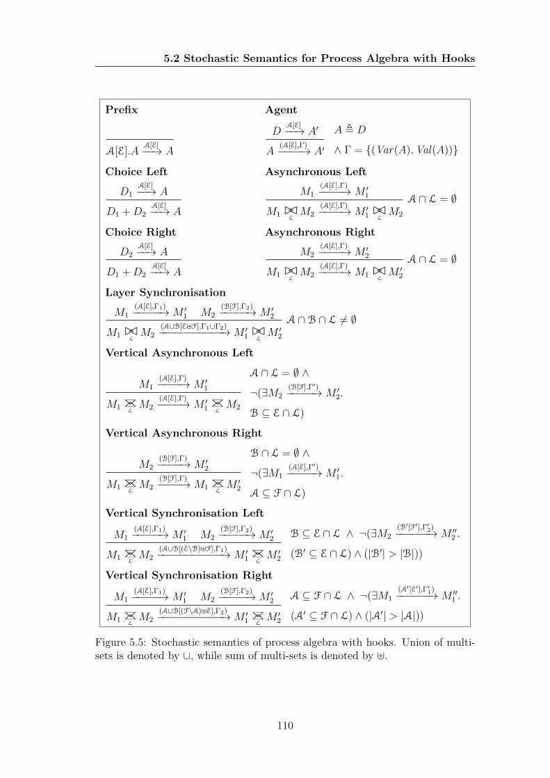
5.2 Stochastic Semantics for Process Algebra with Hooks
Prefix Agent
A[E].AA[E]−−→ A
DA[E]−−→ A′
A(A[E],Γ)−−−−→ A′
A , D
∧ Γ = {(Var(A),Val(A))}
Choice Left Asynchronous Left
D1A[E]−−→ A
D1 +D2A[E]−−→ A
M1(A[E],Γ)−−−−→M ′
1
M1 BCLM2
(A[E],Γ)−−−−→M ′1BCLM2
A ∩ L = ∅
Choice Right Asynchronous Right
D2A[E]−−→ A
D1 +D2A[E]−−→ A
M2(A[E],Γ)−−−−→M ′
2
M1 BCLM2
(A[E],Γ)−−−−→M1 BCLM ′
2
A ∩ L = ∅
Layer Synchronisation
M1(A[E],Γ1)−−−−−→M ′
1 M2(B[F],Γ2)−−−−−→M ′
2
M1 BCLM2
(A∪B[E]F],Γ1∪Γ2)−−−−−−−−−−−→M ′1BCLM ′
2
A ∩B ∩ L 6= ∅
Vertical Asynchronous Left
M1(A[E],Γ)−−−−→M ′
1
M1 BC
LM2
(A[E],Γ)−−−−→M ′1 BC
LM2
A ∩ L = ∅ ∧
¬(∃M2(B[F],Γ′)−−−−−→M ′
2.
B ⊆ E ∩ L)
Vertical Asynchronous Right
M2(B[F],Γ)−−−−→M ′
2
M1 BC
LM2
(B[F],Γ)−−−−→M1 BC
LM ′
2
B ∩ L = ∅ ∧
¬(∃M1(A[E],Γ′)−−−−−→M ′
1.
A ⊆ F ∩ L)
Vertical Synchronisation Left
M1(A[E],Γ1)−−−−−→M ′
1 M2(B[F],Γ2)−−−−−→M ′
2
M1 BC
LM2
(A∪B[(E\B)]F],Γ1)−−−−−−−−−−−→M ′1 BC
LM ′
2
B ⊆ E ∩ L ∧ ¬(∃M2
(B′[F′],Γ′2)−−−−−−→M ′′
2 .
(B′ ⊆ E ∩ L) ∧ (|B′| > |B|))
Vertical Synchronisation Right
M1(A[E],Γ1)−−−−−→M ′
1 M2(B[F],Γ2)−−−−−→M ′
2
M1 BC
LM2
(A∪B[(F\A)]E],Γ2)−−−−−−−−−−−→M ′1 BC
LM ′
2
A ⊆ F ∩ L ∧ ¬(∃M1
(A′[E′],Γ′1)−−−−−−→M ′′
1 .
(A′ ⊆ F ∩ L) ∧ (|A′| > |A|))
Figure 5.5: Stochastic semantics of process algebra with hooks. Union of multi-sets is denoted by ∪, while sum of multi-sets is denoted by ].
110
5.2 Stochastic Semantics for Process Algebra with Hooks
Definition 5.4 Derivative Set. The derivative set of a model process M ∈ Pmis denoted by ds(M) and is defined as the smallest set of model processes such
that:
• M ∈ ds(M);
• if Mi ∈ ds(M) and Mi(A[E],Γ)−−−−→Mj then Mj ∈ ds(M).
Definition 5.5 Current moves of a definition process. The multi set of moves
that D ∈ Pd can perform is denoted by Moves(D) and is defined as:
• Moves(nil) = {||};
• Moves(A[E].A) = {|(A[E], A)|};
• Moves(D1 +D2) = Moves(D1) ]Moves(D2).
with {||} delimiting a multi set and ] the sum of multi sets.
Definition 5.6 Current moves of a model process. The multi set of moves that
M ∈ Pm can perform is denoted by Moves(M) and is defined as:
((A[E],Γ),M ′) ∈ Moves(M) iff M(A[E],Γ)−−−−→ M ′, with the same multiplicity as
the number of derivation trees that can derive M(A[E],Γ)−−−−→M ′ using the derivation
rules in Figure 5.5.
Definition 5.7 Current composed actions for definition processes. The multi
set of composed actions that D ∈ Pd can perform is denoted by CompAct(D)
and is defined as:
CompAct(D) = {|A[E] | (A[E], A) ∈Moves(D)|}
Definition 5.8 Current activities for model Processes. The multi set of activities
that M ∈ Pm can perform is denoted by Activities(M) and is defined as:
Activities(M) = {|(A[E],Γ) | ((A[E],Γ),M ′) ∈Moves(M)|}
111
5.2 Stochastic Semantics for Process Algebra with Hooks
Definition 5.9 Activity set. The multi set of activities that a model process
M ∈ Pm and its derivatives can perform is given by:
−−−−−−→Activities(M) =
⊎Mi∈ds(M)
Activities(Mi)
Definition 5.10 Derivation graph. Given a model component M ∈ Pm, the
derivation graph D(M) is the labelled directed graph with:
• set of nodes ds(M);
• multi set of transition labels−−−−−−→Activities(M);
• multi set of labelled transitions→⊆ ds(M)×−−−−−−→Activities(M)×ds(M). Given
M ′ ∈ ds(M), (M ′,A[E],Γ,M ′′) ∈→ iff M ′ (A[E],Γ)−−−−→ M ′′, with the same
multiplicity of ((A[E],Γ),M ′′) in Moves(M ′).
5.2.2 Rating sPAH models
In analogy with the functional rate evaluation in sSPA (Sections 3.2.3 and 3.2.4),
we proceed now to the definition of a sPAH model, the rating routines and the
rated derivation graph for sPAH models.
Definition 5.11 sPAH model. An sPAH model is a tuple:
(AgentDef ,M,Actions,Names,F,Γ, Participants,Var ,Val)
where:
• AgentDef is the finite set of agent definitions {A1 , D1, A2 , D2, . . . };
• M is the initial state of the model, with M ∈ Pm;
• Actions is the finite set of actions;
• Names is the finite set of parameter names;
• F is the finite set of functional rates;
• Γ is the finite set of constant model parameters, with Γ ⊆ Names× R;
112
5.2 Stochastic Semantics for Process Algebra with Hooks
• Participants is the finite set of sets of participants;
• Var and Val are the functions associating agents with variables (i.e. pa-
rameter names) and values, with Var : Pm → Names and Val : Pm → R.
In order to ensure correct and unambiguous rate evaluation and to guarantee
that congruence relations (Chapter 6) can be defined on sPAH processes, we
employ the following additional constraints:
• each functional rate fa ∈ F is associated with a set of participants pa ⊆Names;
• at any time only one agent can be associated with a certain variable;
• whenever an agent A performs an action (application of derivation rule
Agent), the resulting agent A′ will be associated with the same variable A
is associated with;
• only agents associated with variables in pa can perform action a. This is
to prevent an additional synchronisation via BCL
changing a closed activity
into an open activity, due to an increase of the size of Γ.
• actions used as hook actions must not be associated with functional rates;
• an activity (A[E],Γ) can be rated only if Γ contains exactly the variables
in pa and A contains exactly one action name a such that fa ∈ F. Such
activity is called closed. An activity that is not closed is called open;
• if more than one transition from a certain state is associated with the same
functional rate, the evaluated rate has to be normalised, i.e. it has to be
divided by the number of such transitions.
The above constraints are formalised by the following definitions. With these
we can define a rated derivation graph.
Definition 5.12 Well formed sPAH model. A sPAH model is well formed if and
only if:
113
5.2 Stochastic Semantics for Process Algebra with Hooks
1. Given a model process as a cooperation of agents of the form
A1 ◦ A2 ◦ · · · ◦ An
then ∀Ai, Aj if i 6= j then Var(Aj) 6= Var(Aj), where ◦ is either a vertical
or horizontal cooperation;
2. Given a definition of an agent A as a choice of sequential actions of the form
A ,∑i
ai.Ai
then ∀Ai Var(A) = Var(Ai);
3. ∀a s.t. fa ∈ F, ∀A agents
∃(A[E],Γ) ∈−−−−−−→Activities(A) s.t. a ∈ A ∪ E⇔ Var(A) ∈ pa
Moreover, whenever M1 BCLM2 then ∀a s.t. fa ∈ F
a ∈ L⇔ ∃(A[E],Γ) ∈−−−−−−→Activities(M1),
(B[F],Γ′) ∈−−−−−−→Activities(M2) s.t. a ∈ A ∧ a ∈ B
4. hook actions are not associated with functional rates:
∀A agents, ∀(A[E],Γ) ∈−−−−−−→Activities(A), ∀a s.t. fa ∈ F, a 6∈ E
5. ∀A agents defined as
A ,∑i
Ai[Hi].Ai
∀a s.t. fa ∈ F, if a ∈ Ai then Ai = {|a|}.
Definition 5.12 ensures that whenever M(A[H],Γ)−−−−−→M ′ then either ∀a s.t. fa ∈ F
a 6∈ A or ∃!a s.t. fa ∈ F and a ∈ A. In other words, for every valid transition,
the set of layer actions contains at most one action associated with a functional
rate.
114
5.2 Stochastic Semantics for Process Algebra with Hooks
Definition 5.13 Function envVar. The function envV ar extracts the set of
variables in an environment Γ ⊆ Names× R:
envV ar(Γ) = ({i | (i, k) ∈ Γ})
Definition 5.14 Function activeActions. The function activeActions selects
actions a such that a functional rate in the set F is associated with a, i.e. fa ∈ F,
from a action set A ⊆ Actions:
activeActions(A)F = ({a | a ∈ A ∧ fa ∈ F})
Definition 5.15 Open activity. An open activity is an activity (A[E],Γ) where
at least one of the following conditions are true:
• the number of active actions in A is different from one, i.e.
|activeActions(A)F| 6= 1;
• if |activeActions(A)F| = 1 and a ∈ activeActions(A)F, Γ does not contain
the exact variables present in the participant set pa, i.e. pa 6= envV ar(Γ).
Definition 5.16 Function openActivities. The function openActivities selects
open activities from a set of activities A ⊆ 2Actions × 2Actions × 2Names×R:
openActivities(A) ={∣∣∣∣(A[E],Γ)
∣∣∣∣ (A[E],Γ) ∈ A ∧ (|activeActions(A)F| 6= 1
∨(activeActions(A)F = {a} ∧ pa 6= envV ar(Γ)))
∣∣∣∣}
Definition 5.17 Current open activities. Given a model process M ∈ Pm, the
multi set of open activities that P can perform is defined as:
OpenAct(M) = openActivities(Activities(M))
Definition 5.18 Open activity set. The multi set of all open activities that a
model process M ∈ Pm can perform is given by:
−−−−−−→OpenAct(M) = openActivities(
−−−−−−→Activities(M))
115
5.2 Stochastic Semantics for Process Algebra with Hooks
Definition 5.19 Closed activity. A closed activity is an activity (A[E],Γ) where:
• |activeActions(A)F| = 1, a ∈ activeActions(A)F and Γ contains the exact
variables present in the participant set pa, i.e. pa = envV ar(Γ).
Definition 5.20 Function closedActivities. The function closedActivities se-
lects closed activities from a set of activities A ⊆ 2Actions × 2Actions × 2Names×R:
closedActivities(A) = (A \ openActivities(A))
Definition 5.21 Current closed activities. Given a model process M ∈ Pm, the
multi set of closed activities that M can perform is defined as:
ClosedAct(M) = closedActivities(Activities(M))
Definition 5.22 Closed activity set. The multi set of all closed activities that a
model process M ∈ Pm can perform is given by:
−−−−−−−→ClosedAct(M) = closedActivities(
−−−−−−→Activities(M))
Definition 5.23 Open moves of a model process. Given a model process M ∈Pm, the multi set of open moves of M , denoted OpenMoves(M), is defined as:
OpenMoves(M) = {|(a,M ′) | (a,M ′) ∈Moves(M) ∧ a ∈ OpenAct(M))|}
Definition 5.24 Rated activity. The pair (A[E], r) such that A,E ⊆ Actions
and r ∈ R>0 is called a rated activity.
Definition 5.25 Function rateActivities. Given an environment Γ ⊆ Names×R, rateActivities converts a set of activities A ⊆ 2Actions×2Actions×2Names×R into
a set of rated activities B ⊆ 2Actions × 2Actions × R:
rateActivities(Γ)(A) ={∣∣∣∣(A[E], r)
∣∣∣∣ (A[E],Γ′) ∈ A ∧ {a} = activeActions(A)F
∧ Γ ∪ Γ′ ` fa → k ∧ ra = k/π(A, (a,Γ′)) ∧ fa ∈ F
∣∣∣∣}
116
5.2 Stochastic Semantics for Process Algebra with Hooks
where π(A, (a,Γ′)) returns the number of occurrences of (A[E],Γ′) in the multi
set A such that {a} = activeActions(A)F.
Definition 5.26 Current rated activities. Given a model process M ∈ Pm and
an environment Γ ⊆ Names× R, the multi set of rated activities that M can
perform is defined as:
RatedAct(M)Γ = rateActivities(Γ)(ClosedAct(M))
RatedAct(M)Γ can be written RatedAct(M) if Γ is clear from the context.
Definition 5.27 Rated activity set. Given an environment Γ ⊆ Names× R,
the multi set of rated activities that a model process M ∈ Pm and its derivatives
can perform is given by:
−−−−−−→RatedAct(M)Γ = rateActivities(Γ)(
−−−−−−−→ClosedAct(M))
−−−−−−→RatedAct(M)Γ can be written
−−−−−−→RatedAct(M) if Γ is clear from the context.
Definition 5.28 Rated moves of a model process. Given a model process M ∈Pm and an environment Γ ⊆ Names × R, the multi set of rated moves of M ,
denoted RatedMoves(M)Γ, is defined as:
RatedMoves(M)Γ = {|((A[E], r),M ′) | ((A[E],Γ′),M ′) ∈Moves(M ′) ∧ (A[E],Γ′)
∈ ClosedAct(M) ∧ {|((A[E], k))|} = rateActivities(Γ)({|(A[E],Γ′)|})∧
activeActions(A)F = a ∧ r = k/π(ClosedAct(M), (a,Γ′))|}
Definition 5.29 Rated transitions. Given M ∈ Pm and Γ ⊆ Names× R,
M(A[E],r)−−−−→Γ M ′ is a valid rated transition iff M
(A[E],Γ′)−−−−−→ M ′, (A[E],Γ′) ∈ClosedAct(M), {|((A[E], k))|} = rateActivities(Γ)({|(A[E],Γ′)|}),activeActions(A)F = a and r = k/π(ClosedAct(M), (a,Γ′)).
Definition 5.30 Rated derivation graph. Given a model process M ∈ Pm and an
environment Γ ⊆ Names× R, the rated derivation graph Dr(M)Γ is the labelled
117
5.2 Stochastic Semantics for Process Algebra with Hooks
directed graph with:
• set of nodes ds(M);
• multi set of transition labels−−−−−−→RatedAct(M)Γ;
• multi set of labelled transitions →r⊆ ds(M) ×−−−−−−→RatedAct(M)Γ × ds(M).
Given M ′ ∈ ds(M), (M ′,A[E], ra,M′′) ∈→r iff M ′ (A[E],ra)−−−−−→Γ M
′′, with the
same multiplicity of ((A[E], ra),M′′) in RatedMoves(M ′)Γ.
• multi set of labelled transitions→o⊆ ds(M)×−−−−−−→OpenAct(M)×ds(M). Given
M ′ ∈ ds(M), (M ′,A[E],Γ′,M ′′) ∈→o iff M ′ (A[E],Γ′)−−−−−→ M ′′ and (A[E],Γ′) ∈OpenAct(M), with the same multiplicity of ((A[E],Γ′),M ′′) in Moves(M ′).
Dr(M)Γ can be written Dr(M) if Γ is clear from the context.
In the following sections we illustrate the use of sPAH, augmenting examples
of previous sections with functional rates.
5.2.3 Stochastic Process Algebra with Hooks and a Three
Layers Example
In this section we show how the example in Section 5.1.2 can be augmented with
functional rates. The processes are:
A0 , a.A1 + f.A1 B0 , c.B1 + e.B1 P0 , p.P1
A1 , a[p].A2 + b.A0 B1 , c[p].B2 + d.B0 P1 , q.P0 + p[x].P2 + {|p, q|}.P1
+f [p].A2 + e.A0 +e[p].B2 + f.B0 P2 , q[y].P1
A2 , b[q].A1 + e[q].A1 B2 , d[q].B1 + f [q].B1
CellM , move.CellM + x.CellA CellA , absorb.CellA + y.CellM
The initial state of the model is given by:
((A0 BCLB0) BC
HP0) BC
KC1
where L = {|e, f |}, H = {|p, q|} and K = {|x, y|}. Variables and values:
118
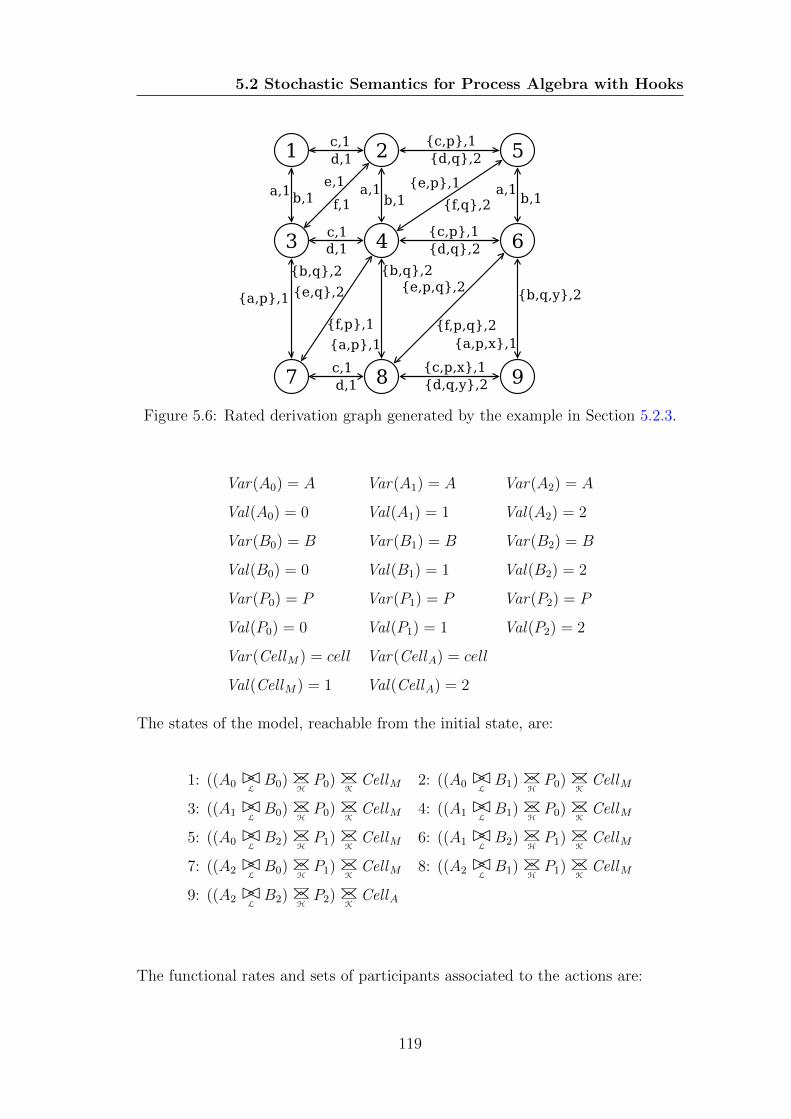
5.2 Stochastic Semantics for Process Algebra with Hooks
Figure 5.6: Rated derivation graph generated by the example in Section 5.2.3.
Var(A0) = A Var(A1) = A Var(A2) = A
Val(A0) = 0 Val(A1) = 1 Val(A2) = 2
Var(B0) = B Var(B1) = B Var(B2) = B
Val(B0) = 0 Val(B1) = 1 Val(B2) = 2
Var(P0) = P Var(P1) = P Var(P2) = P
Val(P0) = 0 Val(P1) = 1 Val(P2) = 2
Var(CellM) = cell Var(CellA) = cell
Val(CellM) = 1 Val(CellA) = 2
The states of the model, reachable from the initial state, are:
1: ((A0 BCLB0) BC
HP0) BC
KCellM 2: ((A0 BC
LB1) BC
HP0) BC
KCellM
3: ((A1 BCLB0) BC
HP0) BC
KCellM 4: ((A1 BC
LB1) BC
HP0) BC
KCellM
5: ((A0 BCLB2) BC
HP1) BC
KCellM 6: ((A1 BC
LB2) BC
HP1) BC
KCellM
7: ((A2 BCLB0) BC
HP1) BC
KCellM 8: ((A2 BC
LB1) BC
HP1) BC
KCellM
9: ((A2 BCLB2) BC
HP2) BC
KCellA
The functional rates and sets of participants associated to the actions are:
119
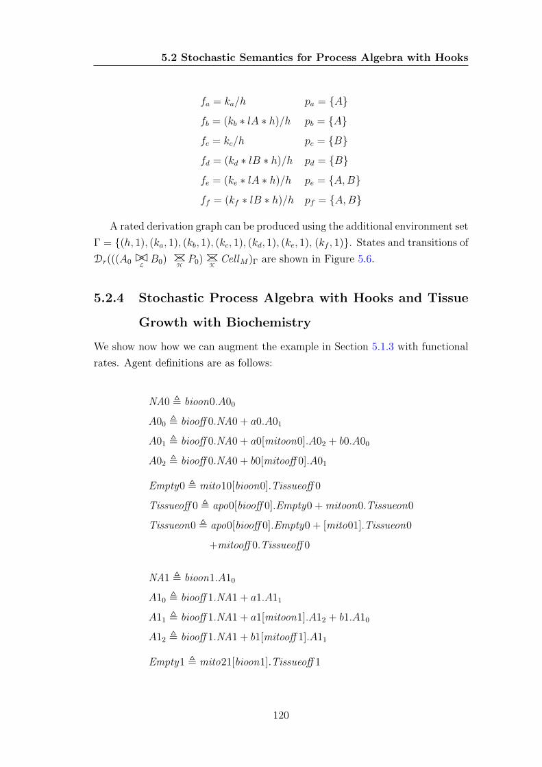
5.2 Stochastic Semantics for Process Algebra with Hooks
fa = ka/h pa = {A}
fb = (kb ∗ lA ∗ h)/h pb = {A}
fc = kc/h pc = {B}
fd = (kd ∗ lB ∗ h)/h pd = {B}
fe = (ke ∗ lA ∗ h)/h pe = {A,B}
ff = (kf ∗ lB ∗ h)/h pf = {A,B}
A rated derivation graph can be produced using the additional environment set
Γ = {(h, 1), (ka, 1), (kb, 1), (kc, 1), (kd, 1), (ke, 1), (kf , 1)}. States and transitions of
Dr(((A0 BCLB0) BC
HP0) BC
KCellM)Γ are shown in Figure 5.6.
5.2.4 Stochastic Process Algebra with Hooks and Tissue
Growth with Biochemistry
We show now how we can augment the example in Section 5.1.3 with functional
rates. Agent definitions are as follows:
NA0 , bioon0.A00
A00 , biooff 0.NA0 + a0.A01
A01 , biooff 0.NA0 + a0[mitoon0].A02 + b0.A00
A02 , biooff 0.NA0 + b0[mitooff 0].A01
Empty0 , mito10[bioon0].Tissueoff 0
Tissueoff 0 , apo0[biooff 0].Empty0 + mitoon0.Tissueon0
Tissueon0 , apo0[biooff 0].Empty0 + [mito01].Tissueon0
+mitooff 0.Tissueoff 0
NA1 , bioon1.A10
A10 , biooff 1.NA1 + a1.A11
A11 , biooff 1.NA1 + a1[mitoon1].A12 + b1.A10
A12 , biooff 1.NA1 + b1[mitooff 1].A11
Empty1 , mito21[bioon1].Tissueoff 1
120
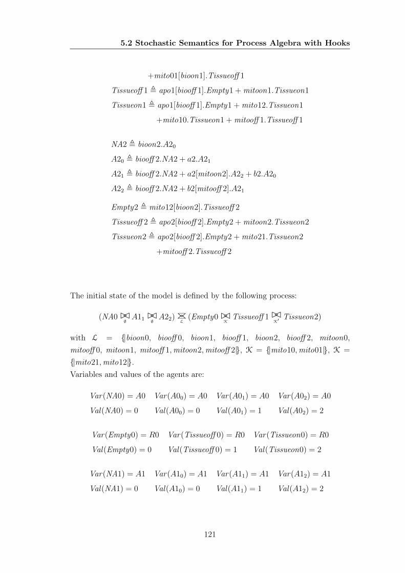
5.2 Stochastic Semantics for Process Algebra with Hooks
+mito01[bioon1].Tissueoff 1
Tissueoff 1 , apo1[biooff 1].Empty1 + mitoon1.Tissueon1
Tissueon1 , apo1[biooff 1].Empty1 + mito12.Tissueon1
+mito10.Tissueon1 + mitooff 1.Tissueoff 1
NA2 , bioon2.A20
A20 , biooff 2.NA2 + a2.A21
A21 , biooff 2.NA2 + a2[mitoon2].A22 + b2.A20
A22 , biooff 2.NA2 + b2[mitooff 2].A21
Empty2 , mito12[bioon2].Tissueoff 2
Tissueoff 2 , apo2[biooff 2].Empty2 + mitoon2.Tissueon2
Tissueon2 , apo2[biooff 2].Empty2 + mito21.Tissueon2
+mitooff 2.Tissueoff 2
The initial state of the model is defined by the following process:
(NA0BC∅A11 BC∅ A22) BC
L(Empty0BC
KTissueoff 1BC
K′Tissueon2)
with L = {|bioon0, biooff 0, bioon1, biooff 1, bioon2, biooff 2, mitoon0,
mitooff 0, mitoon1, mitooff 1,mitoon2,mitooff 2|}, K = {|mito10,mito01|}, K =
{|mito21,mito12|}.Variables and values of the agents are:
Var(NA0) = A0 Var(A00) = A0 Var(A01) = A0 Var(A02) = A0
Val(NA0) = 0 Val(A00) = 0 Val(A01) = 1 Val(A02) = 2
Var(Empty0) = R0 Var(Tissueoff 0) = R0 Var(Tissueon0) = R0
Val(Empty0) = 0 Val(Tissueoff 0) = 1 Val(Tissueon0) = 2
Var(NA1) = A1 Var(A10) = A1 Var(A11) = A1 Var(A12) = A1
Val(NA1) = 0 Val(A10) = 0 Val(A11) = 1 Val(A12) = 2
121
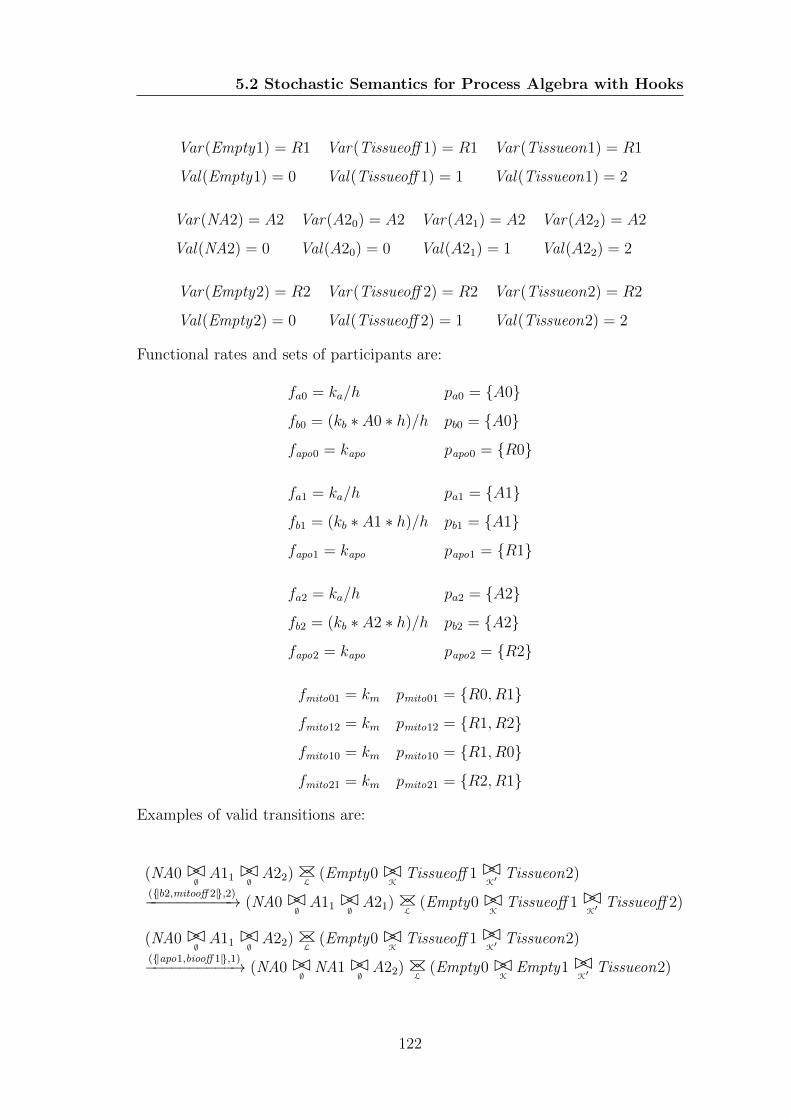
5.2 Stochastic Semantics for Process Algebra with Hooks
Var(Empty1) = R1 Var(Tissueoff 1) = R1 Var(Tissueon1) = R1
Val(Empty1) = 0 Val(Tissueoff 1) = 1 Val(Tissueon1) = 2
Var(NA2) = A2 Var(A20) = A2 Var(A21) = A2 Var(A22) = A2
Val(NA2) = 0 Val(A20) = 0 Val(A21) = 1 Val(A22) = 2
Var(Empty2) = R2 Var(Tissueoff 2) = R2 Var(Tissueon2) = R2
Val(Empty2) = 0 Val(Tissueoff 2) = 1 Val(Tissueon2) = 2
Functional rates and sets of participants are:
fa0 = ka/h pa0 = {A0}
fb0 = (kb ∗ A0 ∗ h)/h pb0 = {A0}
fapo0 = kapo papo0 = {R0}
fa1 = ka/h pa1 = {A1}
fb1 = (kb ∗ A1 ∗ h)/h pb1 = {A1}
fapo1 = kapo papo1 = {R1}
fa2 = ka/h pa2 = {A2}
fb2 = (kb ∗ A2 ∗ h)/h pb2 = {A2}
fapo2 = kapo papo2 = {R2}
fmito01 = km pmito01 = {R0, R1}
fmito12 = km pmito12 = {R1, R2}
fmito10 = km pmito10 = {R1, R0}
fmito21 = km pmito21 = {R2, R1}
Examples of valid transitions are:
(NA0BC∅A11 BC∅ A22) BC
L(Empty0BC
KTissueoff 1BC
K′Tissueon2)
({|b2,mitooff 2|},2)−−−−−−−−−−→ (NA0BC∅A11 BC∅ A21) BC
L(Empty0BC
KTissueoff 1BC
K′Tissueoff 2)
(NA0BC∅A11 BC∅ A22) BC
L(Empty0BC
KTissueoff 1BC
K′Tissueon2)
({|apo1,biooff 1|},1)−−−−−−−−−−→ (NA0BC∅
NA1BC∅A22) BC
L(Empty0BC
KEmpty1BC
K′Tissueon2)
122
5.3 Summary
5.3 Summary
In this chapter we have introduced process algebra with hooks, a novel process
algebra designed for multi-scale modelling of biological systems. The distinctive
features of the algebra are composed actions and a new vertical operator. These
new elements ensure that both the effects that an event produces at the scale
where it originates and the effects that propagate to other scales can be mod-
elled with a single transition. We illustrated the use of the algebra with several
examples and we compared it with process algebra with priorities, illustrating
how the former addresses the criticisms we highlighted in the latter. Finally, we
developed a stochastic semantics for process algebra with hooks, which supports
functional rates. This has been done following the approach to functional rates
we developed in Chapter 3.
In the next chapter we introduce three fundamental equivalence relations for
process algebra with hooks.
123
Chapter 6
Relations for Stochastic Process
Algebra with Hooks
In this chapter we introduce three equivalence relations for stochastic process
algebra with hooks: isomorphism (≡), T-isomorphism (≡T) and Markovian T-
bisimulation ('T). The last two equivalences relate processes at specified scales.
In Section 6.1 we introduce the idea behind these relations and discuss the con-
cept of the filtering of activities. In Section 6.2 we define the relations and give
fundamental results such as equational laws and proofs of congruence. Finally,
we discuss the practical use of these relations in Section 6.2.3.
6.1 Relating Biological Systems at Specified Scales
It is common practice to describe the behaviour of a biological system at a specific
scale. When we do that, details of other scales are neglected as much as possible,
only referred to when they are strictly necessary. For example, we compare the
behaviour of two distinct populations of cells and observe that they proliferate
at the same speed. The discussion is at the cellular scale, with cells as entities
and the action of proliferation, or cell duplication, as event. Then, we might
investigate further and discover that a cell duplicates in the first population only
when a chemical A is present, in a certain amount. With this new observation, we
are referring to a different scale: the molecular scale. Investigating even further,
we might find that in the second population cell duplication is possible only if
124
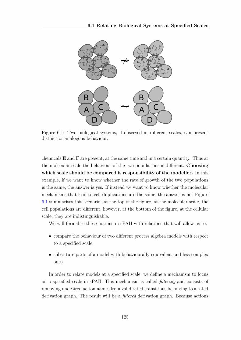
6.1 Relating Biological Systems at Specified Scales
A
BC
D
A B
CDA B
CD
A B
CD
A B
CD
A B
CD
A B
CD
A
BC
D
E
F
G
E
F
G
E
F
GE
F
G
E
F
G
E
F
G
~
~
Figure 6.1: Two biological systems, if observed at different scales, can presentdistinct or analogous behaviour.
chemicals E and F are present, at the same time and in a certain quantity. Thus at
the molecular scale the behaviour of the two populations is different. Choosing
which scale should be compared is responsibility of the modeller. In this
example, if we want to know whether the rate of growth of the two populations
is the same, the answer is yes. If instead we want to know whether the molecular
mechanisms that lead to cell duplications are the same, the answer is no. Figure
6.1 summarises this scenario: at the top of the figure, at the molecular scale, the
cell populations are different, however, at the bottom of the figure, at the cellular
scale, they are indistinguishable.
We will formalise these notions in sPAH with relations that will allow us to:
• compare the behaviour of two different process algebra models with respect
to a specified scale;
• substitute parts of a model with behaviourally equivalent and less complex
ones.
In order to relate models at a specified scale, we define a mechanism to focus
on a specified scale in sPAH. This mechanism is called filtering and consists of
removing undesired action names from valid rated transitions belonging to a rated
derivation graph. The result will be a filtered derivation graph. Because actions
125
6.1 Relating Biological Systems at Specified Scales
are associated with functional rates, removing actions interferes with rating. As
a consequence, rating of transitions should always precede filtering.
In sPAH actions from every scale are collected into a unique action multi-set
that labels valid transitions. If we want to focus on a specific scale, all we need to
do is to keep only the actions pertaining to a given scale. For example, consider
the following rated transition:
M({|a,h,x|}[{|y,z|}],r)−−−−−−−−−−→Γ M
′
From this transition it is possible to infer that actions a, h and x have been
performed, that hook actions y and z have not been used in any synchronisation
and that the rate of the transition is r. Now assume that we are interested
in only the behaviour represented by the actions in T, with T = {|x, y|}. The
corresponding filtered transition should be:
M({|x|},{|y,z|},r)−−−−−−−−→T,Γ M
′
Notice that the rate and the multi-set of hook actions is untouched. Moreover, a
filtered activity is a triple, to distinguish it from a rated activity, which is a pair.
We introduce now the formal definitions of filtered activities, filtered transitions
and filtered derivation graph.
Definition 6.1 Filtered activities. The triple (A,E, r) such that A and E are
multi-sets of actions and r ∈ R>0 is called a filtered activity.
Definition 6.2 Function filterActivities. Given a multi-set of actions T, fil-
terActivities converts a multi-set of rated activities A into a multi-set of filtered
activities:
filterActivities(T)(A) = {|(B,E, r) | (A,E, r) ∈ A ∧B = A ∩ T|}
Definition 6.3 Current filtered composed actions of a definition process. Given
a multi-set of actions T, the multi-set of filtered composed actions that D ∈ Pdcan perform is denoted by FiltCompAct(D)T and is defined as:
FiltCompAct(D)T = {|(B,E) | A[E] ∈ CompAct(D) ∧B = A ∩ T|}
126
6.1 Relating Biological Systems at Specified Scales
Definition 6.4 Current filtered activities of a model process. Given a multi-
set of actions T and an environment Γ ⊆ Names × R, the multi-set of filtered
activities that a model process M ∈ Pm can perform is denoted by FiltAct(M)T,Γ
and is defined as:
FiltAct(M)T,Γ = filterActivities(T)(RatedAct(M)Γ)
Definition 6.5 Filtered activity set. Given a multi-set of actions T and an
environment Γ ⊆ Names × R, the multi-set of filtered activities that a model
process M ∈ Pm and its derivatives can perform is denoted by−−−−−→FiltAct(M)T,Γ
and is defined as:
−−−−−→FiltAct(M)T,Γ = filterActivities(T)(
−−−−−−−−−→RatedAct(M)Γ)
Definition 6.6 Filtered moves of a definition process. Given a multi-set of
actions T, the multi-set of moves that a definition process D ∈ Pd can perform is
denoted by FiltMovesDT and is defined as:
FiltMoves(D)T = {|((B,E), A) | (A[E], A) ∈Moves(D) ∧B = A ∩ T|}
Definition 6.7 Filtered moves of a model process. Given a multi-set of actions
T and an environment Γ ⊆ Names × R, the multi-set of moves that a model
process M ∈ Pm can perform is denoted by FiltMovesMT,Γ and is defined as:
FiltMoves(M)T,Γ = {|((B,E, r), A) | ((A[E], r), A) ∈ RatedMoves(M)∧B = A∩T|}
Definition 6.8 Filtered transitions of a definition process. Given D ∈ Pd and a
multi-set of actions T, D(B,E)−−−→T A is a valid filtered transition iff D
A[E]−−→ A for
some A such that B = A ∩ T.
Definition 6.9 Filtered transitions of a model process. Given M ∈ Pm, a multi-
set of actions T and an environment Γ ⊆ Names× R, M(B,E,r)−−−−→T,Γ M
′ is a valid
filtered transition iff M(A[E],r)−−−−→Γ M
′ for some A such that B = A ∩ T.
127
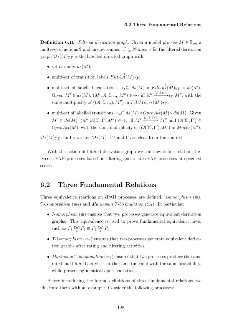
6.2 Three Fundamental Relations
Definition 6.10 Filtered derivation graph. Given a model process M ∈ Pm, a
multi-set of actions T and an environment Γ ⊆ Names× R, the filtered derivation
graph Df (M)T,Γ is the labelled directed graph with:
• set of nodes ds(M);
• multi-set of transition labels−−−−−→FiltAct(M)T,Γ;
• multi-set of labelled transitions →f⊆ ds(M) ×−−−−−→FiltAct(M)T,Γ × ds(M).
Given M ′ ∈ ds(M), (M ′,A,E, ra,M′′) ∈→f iff M ′ (A,E,ra)−−−−→T,Γ M
′′, with the
same multiplicity of ((A,E, ra),M′′) in FiltMoves(M ′)T,Γ.
• multi-set of labelled transitions→o⊆ ds(M)×−−−−−−→OpenAct(M)×ds(M). Given
M ′ ∈ ds(M), (M ′,A[E],Γ′,M ′′) ∈→o iff M ′ (A[E],Γ′)−−−−−→ M ′′ and (A[E],Γ′) ∈OpenAct(M), with the same multiplicity of ((A[E],Γ′),M ′′) in Moves(M ′).
Df (M)T,Γ can be written Df (M) if T and Γ are clear from the context.
With the notion of filtered derivation graph we can now define relations be-
tween sPAH processes based on filtering and relate sPAH processes at specified
scales.
6.2 Three Fundamental Relations
Three equivalence relations on sPAH processes are defined: isomorphism (≡),
T-isomorphism (≡T) and Markovian T-bisimulation ('T). In particular:
• Isomorphism (≡) ensures that two processes generate equivalent derivation
graphs. This equivalence is used to prove fundamental equivalence laws,
such as P1 BCLP2 ≡ P2 BC
LP1;
• T-isomorphism (≡T) ensures that two processes generate equivalent deriva-
tion graphs after rating and filtering activities;
• Markovian T-bisimulation ('T) ensures that two processes produce the same
rated and filtered activities at the same time and with the same probability,
while presenting identical open transitions.
Before introducing the formal definitions of three fundamental relations, we
illustrate them with an example. Consider the following processes:
128
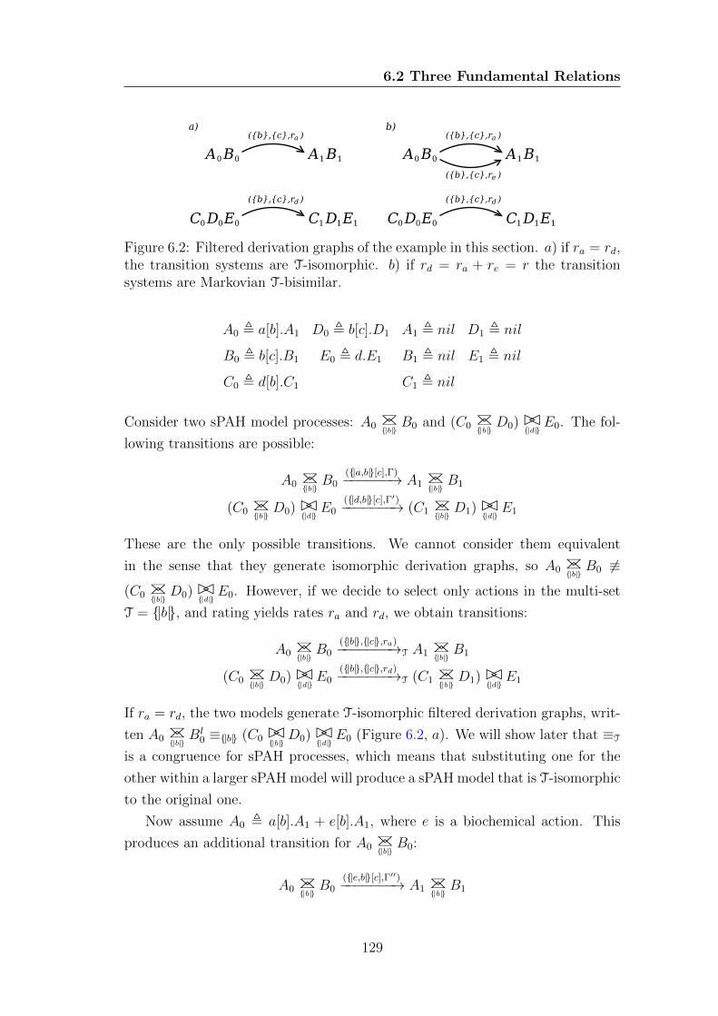
6.2 Three Fundamental Relations
Figure 6.2: Filtered derivation graphs of the example in this section. a) if ra = rd,the transition systems are T-isomorphic. b) if rd = ra + re = r the transitionsystems are Markovian T-bisimilar.
A0 , a[b].A1 D0 , b[c].D1 A1 , nil D1 , nil
B0 , b[c].B1 E0 , d.E1 B1 , nil E1 , nil
C0 , d[b].C1 C1 , nil
Consider two sPAH model processes: A0 BC
{|b|}B0 and (C0 BC
{|b|}D0)BC
{|d|}E0. The fol-
lowing transitions are possible:
A0 BC
{|b|}B0
({|a,b|}[c],Γ)−−−−−−→ A1 BC
{|b|}B1
(C0 BC
{|b|}D0)BC
{|d|}E0
({|d,b|}[c],Γ′)−−−−−−−→ (C1 BC
{|b|}D1)BC
{|d|}E1
These are the only possible transitions. We cannot consider them equivalent
in the sense that they generate isomorphic derivation graphs, so A0 BC{|b|}
B0 6≡
(C0 BC
{|b|}D0)BC
{|d|}E0. However, if we decide to select only actions in the multi-set
T = {|b|}, and rating yields rates ra and rd, we obtain transitions:
A0 BC
{|b|}B0
({|b|},{|c|},ra)−−−−−−−→T A1 BC
{|b|}B1
(C0 BC
{|b|}D0)BC
{|d|}E0
({|b|},{|c|},rd)−−−−−−−→T (C1 BC
{|b|}D1)BC
{|d|}E1
If ra = rd, the two models generate T-isomorphic filtered derivation graphs, writ-
ten A0 BC
{|b|}Bl
0 ≡{|b|} (C0 BC{|b|} D0)BC{|d|}
E0 (Figure 6.2, a). We will show later that ≡T
is a congruence for sPAH processes, which means that substituting one for the
other within a larger sPAH model will produce a sPAH model that is T-isomorphic
to the original one.
Now assume A0 , a[b].A1 + e[b].A1, where e is a biochemical action. This
produces an additional transition for A0 BC
{|b|}B0:
A0 BC
{|b|}B0
({|e,b|}[c],Γ′′)−−−−−−−→ A1 BC
{|b|}B1
129
6.2 Three Fundamental Relations
that filtered for {|b|} becomes:
A0 BC
{|b|}B0
({|b|},{|c|},re)−−−−−−−→T A1 BC
{|b|}B1
As a result the two models are no longer T-isomorphic. However, if rd = ra+re =
r, both A0 BCbB0 and (C0 BC
{|b|}D0)BC
{|d|}E0 can move to a terminal state with filtered
set of layer actions {|b|} and set of hook actions {|c|} with a total rate of r. In other
words, the pair ({|b|}, {|c|}) appears on an activity at the same time with the same
probability, implying the two model processes are Markovian T-bisimilar, written
A0 BC
{|b|}B0 '{|b|} (C0 BC
{|b|}D0)BC
{|d|}E0 (Figure 6.2, b). Again, we will demonstrate 'T
is a congruence for process algebra with hooks processes.
In the next two sections we define formally the three equivalence relations and
their fundamental properties.
6.2.1 Isomorphism and (T,Γ)-isomorphism
In this section we define formally isomorphism (≡) and (T,Γ)-isomorphism (≡T,Γ)
on sPAH processes. Two sPAH processes are considered isomorphic if their deriva-
tion graphs are equivalent, i.e. if it is possible to define a bijection F between the
states of the two derivation graphs such that the moves of the image under F of
a state are always identical to the moves of the same states where in each move
the resulting state is replaced by its image under F. A similar definition is given
for (T,Γ)-isomorphism, where a filtered derivation graph is considered instead of
a derivation graph.
In addition we prove that ≡⊂≡T,Γ (Propositions 6.18 and 6.19), we give equa-
tional laws for ≡ (Proposition 6.20) and we show that both ≡ and ≡T,Γ are
congruences (Propositions 6.22 and 6.23).
Definition 6.11 Function apply. Given a function f : P → P and a multi-set
of filtered moves MSet, function apply applies f to MSet in the following way:
apply(f)(MSet) = {|(a, f(P )) | (a, P ) ∈MSet|}
Definition 6.12 Model process isomorphism. A function F: ds(M1)→ ds(M2)
is a model process isomorphism between M1 and M2 (M1,M2 ∈ Pm), if F is
130
6.2 Three Fundamental Relations
bijective and ∀M ′1 ∈ ds(M1),
Moves(F(M ′1)) = apply(F)(Moves(M ′
1))
Definition 6.13 Isomorphic model processes. Two model processes M1,M2 ∈Pm are isomorphic, written M1 ≡M2, if there is a model process isomorphism F
between them such that D(F(M1)) = D(M2).
Definition 6.14 Model process (T,Γ)-isomorphism. Given an environment Γ ⊆Names× R and an action multi-set T, a function F: ds(M1) → ds(M2) is a
model component (T,Γ)-isomorphism between M1 and M2 (M1,M2 ∈ Pm), if F
is bijective and ∀M ′1 ∈ ds(M1),
FiltMoves(F(M ′1))T,Γ = apply(F)(FiltMoves(M ′
1)T,Γ)
and
OpenMoves(F(M ′1)) = apply(F)(OpenMoves(M ′
1))
Definition 6.15 (T,Γ)-isomorphic model processes. Given an environment Γ ⊆Names× R and an action multi-set T, two model processes M1,M2 ∈ Pm are
(T,Γ)-isomorphic, written M1 ≡T,Γ M2, if there is a model component (T,Γ)-
isomorphism F between them such that Df (F(M1))T,Γ = Df (M2)T,Γ.
If Γ is clear from the context, we write M1 ≡T M2 instead of M1 ≡T,Γ M2 and
we say M1 and M2 are T-isomorphic.
Definition 6.16 Isomorphic definition processes. Two definition processesD1, D2 ∈Pd are isomorphic (D1 ≡ D2) iff there exists an bijective function F : ds(D1) →ds(D2) such that ∀A ∈ ds(D1), A ≡ F(A) and
Moves(D2) = apply(F)(Moves(D1))
Definition 6.17 (T,Γ)-isomorphic definition processes. Given a multi-set of
actions T and an environment Γ ⊆ Names×R, two definition processes D1, D2 ∈Pd are (T,Γ)-isomorphic (D1 ≡T,Γ D2) iff there exists an bijective function F :
131
6.2 Three Fundamental Relations
ds(D1)→ ds(D2) such that ∀A ∈ ds(D1), A ≡T,Γ F(A) and
FiltMoves(D2)T = apply(F)(FiltMoves(D1)T)
Proposition 6.18 Given M1,M2 ∈ Pm,
M1 ≡M2 ⇒ ∀ multi-sets of actions T,∀Γ ⊆ Names× R, M1 ≡T,Γ M2
Proof. We just need to prove is that ∀ multi-sets of actions T, ∀Γ ⊆ Names×R,
∀M ′1 ∈ ds(M1) if Moves(F(M ′
1)) = apply(F)(Moves(M ′1)) then
FiltMoves(F(M ′1))T,Γ = apply(F)(FiltMoves(M ′
1)T,Γ)
and
OpenMoves(F(M ′1)) = apply(F)(OpenMoves(M ′
1)
which is trivially true because filtered moves and open moves are derived from
the moves of processes in the same way.
Proposition 6.19 Given D1, D2 ∈ Pd,
D1 ≡ D2 ⇒ ∀ multi-sets of actions T,∀Γ ⊆ Names× R, D1 ≡T,Γ D2
Proof. Observe that if D1 ≡ D2 then there exists an bijective function F :
ds(D1)→ ds(D2) such that ∀A ∈ ds(D1) then A ≡ F(A) and
Moves(D2) = apply(F)(Moves(D1))
This implies that ∀ multi-sets of actions T, ∀Γ ⊆ Names × R, ∀A ∈ ds(D1)
then A ≡T,Γ F(A) because of Proposition 6.18. Moreover, FiltMoves(D2)T =
apply(F)(FiltMoves(D1)T) because filtered moves are derived in the same way
from the moves of processes.
132
6.2 Three Fundamental Relations
Proposition 6.20 Equational laws for isomorphic sPAH processes. The fol-
lowing laws can be proved using the stochastic operational semantics and the
definition of model and definition process isomorphisms. These are only some
examples of equational laws that can be proved on sPAH processes.
1. D1 +D2 ≡ D2 +D1;
2. (D1 +D2) +D3 ≡ D1 + (D2 +D3);
3. M1 BCLM2 ≡M2 BC
LM1;
4. (M1 BCLM2)BC
LM3 ≡M1 BC
L(M2 BC
LM3);
5. M1 BC
LM2 ≡M2 BC
LM1;
6. (M1 BCLM2)BC
KM3 ≡ M1 BC
L(M2 BC
KM3), if ∀(A[E],Γ) ∈
−−−−−−→Activities(M1),
∀(N[H],Γ′′) ∈−−−−−−→Activities(M3), N ∩ (L \K) = ∅ ∧ A ∩ (K \ L) = ∅;
Proof. We prove each law in turn:
1. Moves(D1 + D2) = Moves(D1) ]Moves(D2) = Moves(D2 + D1) with F
the identity function id : Pm → Pm.
2. proof analogous to 1.
3. We choose model process isomorphism F as
∀M ′1BCLM ′
2 ∈ ds(M1 BCLM2), F(M ′
1BCLM ′
2) = M ′2BCLM ′
1
with M ′1 ∈ ds(M1) and M ′
2 ∈ ds(M2). Clearly, because of the symmetry of
operator BCL
,
Moves(F(M ′1BCLM ′
2)) = apply(F)(Moves(M ′1BCLM ′
2))
4. proof analogous to 3.
5. We choose model process isomorphism F as
∀M ′1 BC
LM ′
2 ∈ ds(M1 BC
LM2), F(M ′
1 BC
LM ′
2) = M ′2 BC
LM ′
1
133
6.2 Three Fundamental Relations
with M ′1 ∈ ds(M1) and M ′
2 ∈ ds(M2). Clearly, because of the symmetry of
operator BC
L,
Moves(F(M ′1 BC
LM ′
2)) = apply(F)(Moves(M ′1 BC
LM ′
2))
6. We choose model process isomorphism F as
∀(M ′1BCLM ′
2)BCKM ′
3 ∈ ds((M1 BCLM2)BC
KM3),
F((M ′1BCLM ′
2)BCKM ′
3) = M ′1BCL
(M ′2BCKM ′
3)
with M ′1 ∈ ds(M1), M ′
2 ∈ ds(M2) and M ′3 ∈ ds(M3). Using the additional
conditions of 6. we have
Moves(F((M ′1BCLM ′
2)BCKM ′
3)) = apply(F)((Moves(M ′1BCLM ′
2)BCKM ′
3))
Proposition 6.21 Equational laws for (T,Γ)-isomorphic sPAH processes. Be-
cause of Propositions 6.18 and 6.19, the equational laws for isomorphic sPAH
processes hold as equational laws for (T,Γ)-isomorphic sPAH processes.
Proposition 6.22 Isomorphism as a Congruence. If P1, P2 ∈ P such that
P1 ≡ P2, then
1. A[E].P1 ≡ A[E].P2, with P1, P2 agents
2. P1 +Q ≡ P2 +Q, with P1, P2, Q ∈ Pd
3. P1 BCLQ ≡ P2 BC
LQ, with P1, P2, Q ∈ Pm
4. P1 BC
LQ ≡ P2 BC
LQ, with P1, P2, Q ∈ Pm
Proof. We prove each case in turn:
1. A[E].P1 and A[E].P2 are definition processes. Because P1 ≡ P2 there exists
model process isomorphism F between them such that F(P1) = P2 and
134
6.2 Three Fundamental Relations
P1 ≡ F(P1). Clearly, we have
Moves(A[E].P2) = apply(F)(Moves(A[E].P1))
2. From the assumptions we know that ∃F : ds(P1) → ds(P2) bijective such
that F(P1) = P2 and ∀A ∈ ds(P1), A ≡ F(A) and
Moves(P2) = apply(F)(Moves(P1))
Thus, we need G : ds(P1 + Q) → ds(P2 + Q) bijective such that ∀A ∈ds(P1 +Q), A ≡ F(A) and
Moves(P2 +Q) = apply(G)(Moves(P1 +Q))
We define G as:
G(A) =
A, if Qa−→ A
F(A), if P1a−→ A
Both cases of G ensure that G(A) ≡ A. Finally:
Moves(P2 +Q) = Moves(P2) ]Moves(Q) =
apply(F)(Moves(P1)) ] apply(id)(Moves(Q)) = apply(G)(Moves(P1 +Q))
3. We know there is a model process isomorphism F between P1 and P2. Each
element of ds(P1 BCLQ) has the form P ′1 BCL Q′. We define a model process
isomorphism G as: ∀P ′1 BCL Q′ ∈ ds(P1 BCLQ), with P ′1 ∈ ds(P1) and Q′ ∈
ds(Q),
G(P ′1 BCL Q′) = F(P ′1)BCLQ′
G is a model process isomorphism because F is a model process isomorphism.
135
6.2 Three Fundamental Relations
In fact:
Moves(G(P ′1 BCL Q′)) = Moves(F(P ′1)BCLQ′) =
{|((A[E],Γ), R BCLQ′) | ((A[E],Γ), R) ∈Moves(F(P ′1)) ∧A ∩ L = ∅|}]
{|((A[E],Γ),F(P ′1)BCLQ′′) | ((A[E],Γ), Q′′) ∈Moves(Q′) ∧A ∩ L = ∅|}]
{|((A[E],Γ), R BCLQ′′)) | ((A1[E1],Γ1), R) ∈Moves(F(P ′1))∧
((A2[E2],Γ2), Q′′) ∈Moves(Q′) ∧A1 ∩A2 ∩ L 6= ∅∧
A = A1 ∪A2 ∧ E = E1 ] E2 ∧ Γ = Γ1 ∪ Γ2|} =
{|((A[E],Γ),F(P ′′1 )BCLQ′) | ((A[E],Γ),F(P ′′1 )) ∈ apply(F)(Moves(P ′1))∧
A ∩ L = ∅|}]
{|((A[E],Γ),F(P ′1)BCLQ′′) | ((A[E],Γ), Q′′) ∈ apply(id)(Moves(Q′))∧
A ∩ L = ∅|}]
{|((A[E],Γ),F(P ′′1 )BCLQ′′)) | ((A1[E1],Γ1),F(P ′′1 )) ∈ apply(F)(Moves(P ′1))
∧((A2[E2],Γ2), Q′′) ∈ apply(id)(Moves(Q′)) ∧A1 ∩A2 ∩ L 6= ∅∧
A = A1 ∪A2 ∧ E = E1 ] E2 ∧ Γ = Γ1 ∪ Γ2|} =
apply(G)(Moves(P ′1 BCL Q′)
4. With the same procedure used for 3, we define a model process isomorphism
G as: ∀P ′1 BC
LQ′ ∈ ds(P1 BC
LQ), with P ′1 ∈ ds(P1) and Q′ ∈ ds(Q),
G(P ′1 BC
LQ′) = F(P ′1) BC
LQ′
G is a model process isomorphism because F is a model process isomorphism
and it can be proved in analogy with point 3.
Proposition 6.23 (T,Γ)-isomorphism as a Congruence. If P1, P2 ∈ P such that
P1 ≡T,Γ P2, then
1. A[E].P1 ≡T,Γ A[E].P2, with P1, P2 agents
136
6.2 Three Fundamental Relations
2. P1 +Q ≡T,Γ P2 +Q, with P1, P2, Q ∈ Pd
3. P1 BCLQ ≡T,Γ P2 BC
LQ, with P1, P2, Q ∈ Pm
4. P1 BCLQ ≡T,Γ P2 BC
LQ, with P1, P2, Q ∈ Pm
Proof. Proof of each case:
1. Clearly ds(A[E].P1) = {P1} and ds(A[E].P2) = {P2}. Thus we construct
a bijective function G : ds(A[E].P1) → ds(A[E].P2) as G(P1) = P2, while
we already have as an assumption that P1 ≡T,Γ P2 and so P1 ≡T,Γ G(P1).
Finally, the only filtered composed action possible for both processes is
(A ∩ T)[E]. This implies that
FiltMoves(A[E].P2)T = apply(G)(FiltMoves(A[E].P1)T)
2. We know P1, P2 ∈ Pd and there exists a bijective function F : ds(P1) →ds(P2) s.t. ∀A ∈ ds(P1), A ≡T,Γ F(A) and
FiltMoves(P2)T = apply(F)(FiltMoves(P1)T)
Observe that ds(P1 +Q) = ds(P1)∪ds(Q) and ds(P2 +Q) = ds(P2)∪ds(Q).
We construct G : ds(P1 +Q)→ ds(P2 +Q) as follows:
G(A) =
F(A) if A ∈ ds(P1)
A if A ∈ ds(Q)
this implies that ∀A ∈ ds(P1 +Q), A ≡T,Γ G(A) and
FiltMoves(P2 +Q)T = FiltMoves(P2)T ] FiltMoves(Q)T =
apply(F)(FiltMoves(P1)T) ] apply(id)(FiltMoves(Q)T) =
apply(G)(FiltMoves(P1 +Q)T)
3. We know P1, P2 ∈ Pm, and there exists an bijective function F : ds(P1) →
137
6.2 Three Fundamental Relations
ds(P2) s.t. F(P1) = P2 and ∀P ′ ∈ ds(P1)
FiltMoves(F(P ′))T,Γ = apply(F)(FiltMoves(P ′)T,Γ)
We construct a (T,Γ)-isomorphism G : ds(P1 BCLQ) → ds(P2 BC
LQ) such
that ∀P ′ BCLQ′ ∈ ds(P1 BC
LQ)
FiltMoves(G(P ′ BCLQ′))T,Γ = apply(G)(FiltMoves(P ′ BC
LQ′)T,Γ)
We choose G(P ′ BCLQ′) = F(P ′)BC
LQ′. In fact:
FiltMoves(G(P ′ BCLQ′))T,Γ = FiltMoves(F(P ′)BC
LQ′)T,Γ =
{|(a,R BCLQ′) | (a,R) ∈ FiltMoves(F(P ′))T,Γ|}]
{|(a,F(P ′)BCLQ′′) | (a,Q′′) ∈ FiltMoves(Q′)T,Γ|}]
{|((A,E, r), R BCLQ′′)) | ((A1[E1],Γ1), R) ∈ OpenMoves(F(P ′))∧
((A2[E2],Γ2), Q′′) ∈ OpenMoves(Q′)A1 ∩A2 ∩ L 6= ∅∧
(A1 ∪A2[E1 ] E2],Γ1 ∪ Γ2) ∈ ClosedAct(F(P ′)BCLQ′)∧
{|(A,E, r)|} = filterActivities(T)(rateActivities(Γ)(
{|(A1 ∪A2[E1 ] E2],Γ1 ∪ Γ2)|}))|} =
apply(G)(FiltMoves(P ′ BCLQ′)T,Γ)
Notice that if an activity is filtered it will no longer synchronise via BCL
,
because it is derived from a closed activity and because of condition 3 in
Definition 5.12 (well formed process algebra with hooks models). Moreover,
new filtered moves can be obtained only from the synchronisation of two
open activities which form a single closed activity. The last = is correct
because
FiltMoves(F(P ′))T,Γ = apply(F)(FiltMoves(P ′)T,Γ)
138
6.2 Three Fundamental Relations
and because
OpenMoves(F(P ′)) = apply(F)(OpenMoves(P ′))
4. We know P1, P2 ∈ Pm, and there exists an bijective function F : ds(P1) →ds(P2) s.t. F(P1) = P2 and ∀P ′ ∈ ds(P1)
FiltMoves(F(P ′))T,Γ = apply(F)(FiltMoves(P ′)T,Γ)
We construct a (T,Γ)-isomorphism G : ds(P1 BC
LQ) → ds(P2 BC
LQ) such
that ∀P ′ BC
LQ′ ∈ ds(P1 BC
LQ)
FiltMoves(G(P ′ BC
LQ′))T,Γ = apply(G)(FiltMoves(P ′ BC
LQ′)T,Γ)
We choose G(P ′ BC
LQ′) = F(P ′) BC
LQ′. In fact:
FiltMoves(G(P ′ BC
LQ′))T,Γ = FiltMoves(F(P ′) BC
LQ′)T,Γ =
{|((A,E, r), R BC
LQ′) | ((A,E, r), R) ∈ FiltMoves(F(P ′))T,Γ ∧ ¬(∃B,E′,
Γ′, Q′′ s.t. ((B[E′],Γ′), Q′′) ∈Moves(Q′) ∧B ⊆ E ∩ L)|}]
{|((B,E′, r),F(P ′) BC
LQ′′) | ((B,E′, r), Q′′) ∈ FiltMoves(Q′)T,Γ ∧ ¬(∃A,
E,Γ′, R s.t. ((A[E],Γ′), R) ∈Moves(F(P ′)) ∧A ⊆ E′ ∩ L)|}]
{|((A ∪ (B \ T), (E \B) ] E′, r), R BC
LQ′′) | ((A,E, r), R) ∈
FiltMoves(F(P ′))T,Γ ∧ ((B[E′],Γ2), Q′′) ∈Moves(Q′) ∧B ⊆ E ∩ L∧
¬(∃B′,E′′,Γ′2, Q′′′ s.t. ((B′[E′′],Γ′2), Q′′′) ∈Moves(Q′) ∧B′ ⊆ E ∩ L∧
|B′| > |B|)|}]
139
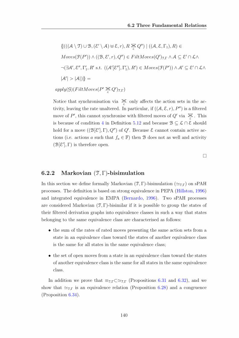
6.2 Three Fundamental Relations
{|(((A \ T) ∪B, (E′ \A) ] E, r), R BC
LQ′′) | ((A,E,Γ1), R) ∈
Moves(F(P ′)) ∧ ((B,E′, r), Q′′) ∈ FiltMoves(Q′)T,Γ ∧A ⊆ E′ ∩ L∧
¬(∃A′,E′′,Γ′1, R′ s.t. ((A′[E′′],Γ′1), R′) ∈Moves(F(P ′)) ∧A′ ⊆ E′ ∩ L∧
|A′| > |A|)|} =
apply(G)(FiltMoves(P ′ BC
LQ′)T,Γ)
Notice that synchronisation via BC
Lonly affects the action sets in the ac-
tivity, leaving the rate unaltered. In particular, if ((A,E, r), P ′′) is a filtered
move of P ′, this cannot synchronise with filtered moves of Q′ via BC
L. This
is because of condition 4 in Definition 5.12 and because B ⊆ L ∩ E should
hold for a move ((B[E′],Γ), Q′′) of Q′. Because E cannot contain active ac-
tions (i.e. actions a such that fa ∈ F) then B does not as well and activity
(B[E′],Γ) is therefore open.
6.2.2 Markovian (T,Γ)-bisimulation
In this section we define formally Markovian (T,Γ)-bisimulation ('T,Γ) on sPAH
processes. The definition is based on strong equivalence in PEPA (Hillston, 1996)
and integrated equivalence in EMPA (Bernardo, 1996). Two sPAH processes
are considered Markovian (T,Γ)-bisimilar if it is possible to group the states of
their filtered derivation graphs into equivalence classes in such a way that states
belonging to the same equivalence class are characterised as follows:
• the sum of the rates of rated moves presenting the same action sets from a
state in an equivalence class toward the states of another equivalence class
is the same for all states in the same equivalence class;
• the set of open moves from a state in an equivalence class toward the states
of another equivalence class is the same for all states in the same equivalence
class.
In addition we prove that ≡T,Γ⊂'T,Γ (Propositions 6.31 and 6.32), and we
show that 'T,Γ is an equivalence relation (Proposition 6.28) and a congruence
(Proposition 6.34).
140
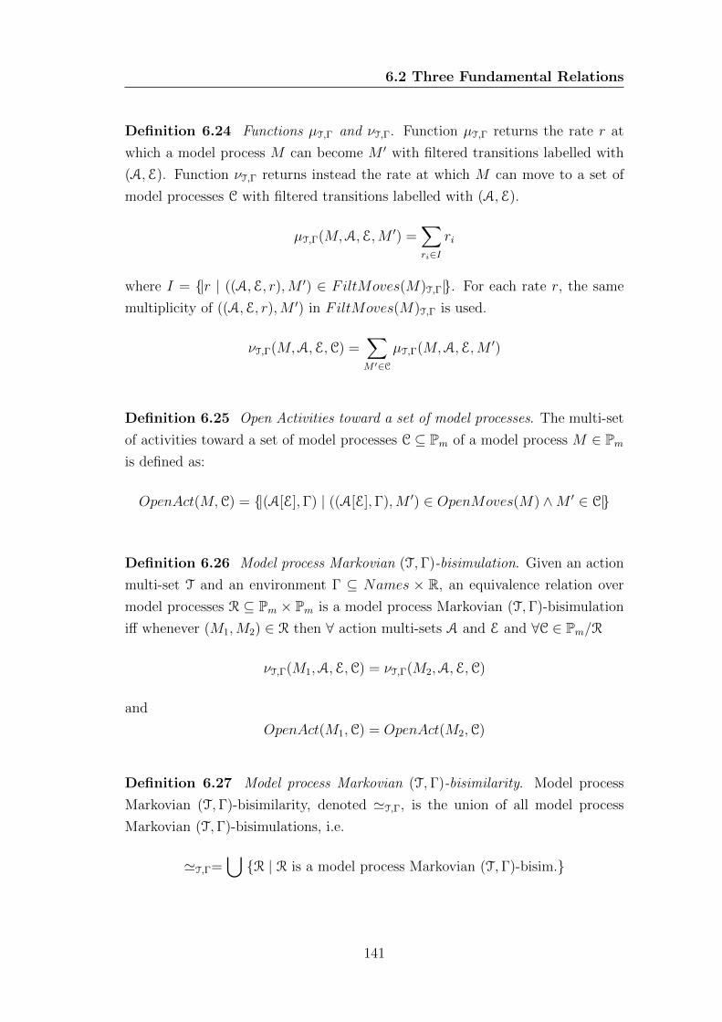
6.2 Three Fundamental Relations
Definition 6.24 Functions µT,Γ and νT,Γ. Function µT,Γ returns the rate r at
which a model process M can become M ′ with filtered transitions labelled with
(A,E). Function νT,Γ returns instead the rate at which M can move to a set of
model processes C with filtered transitions labelled with (A,E).
µT,Γ(M,A,E,M ′) =∑ri∈I
ri
where I = {|r | ((A,E, r),M ′) ∈ FiltMoves(M)T,Γ|}. For each rate r, the same
multiplicity of ((A,E, r),M ′) in FiltMoves(M)T,Γ is used.
νT,Γ(M,A,E,C) =∑M ′∈C
µT,Γ(M,A,E,M ′)
Definition 6.25 Open Activities toward a set of model processes. The multi-set
of activities toward a set of model processes C ⊆ Pm of a model process M ∈ Pmis defined as:
OpenAct(M,C) = {|(A[E],Γ) | ((A[E],Γ),M ′) ∈ OpenMoves(M) ∧M ′ ∈ C|}
Definition 6.26 Model process Markovian (T,Γ)-bisimulation. Given an action
multi-set T and an environment Γ ⊆ Names × R, an equivalence relation over
model processes R ⊆ Pm × Pm is a model process Markovian (T,Γ)-bisimulation
iff whenever (M1,M2) ∈ R then ∀ action multi-sets A and E and ∀C ∈ Pm/R
νT,Γ(M1,A,E,C) = νT,Γ(M2,A,E,C)
and
OpenAct(M1,C) = OpenAct(M2,C)
Definition 6.27 Model process Markovian (T,Γ)-bisimilarity. Model process
Markovian (T,Γ)-bisimilarity, denoted 'T,Γ, is the union of all model process
Markovian (T,Γ)-bisimulations, i.e.
'T,Γ=⋃{R | R is a model process Markovian (T,Γ)-bisim.}
141
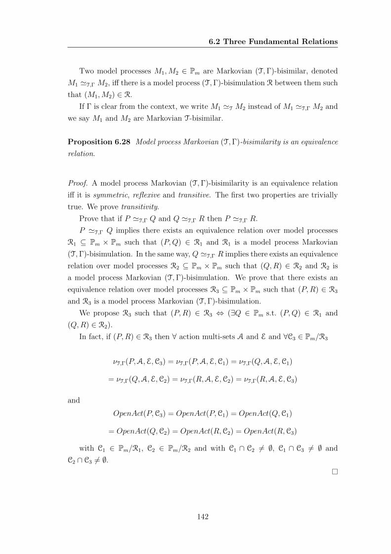
6.2 Three Fundamental Relations
Two model processes M1,M2 ∈ Pm are Markovian (T,Γ)-bisimilar, denoted
M1 'T,Γ M2, iff there is a model process (T,Γ)-bisimulation R between them such
that (M1,M2) ∈ R.
If Γ is clear from the context, we write M1 'T M2 instead of M1 'T,Γ M2 and
we say M1 and M2 are Markovian T-bisimilar.
Proposition 6.28 Model process Markovian (T,Γ)-bisimilarity is an equivalence
relation.
Proof. A model process Markovian (T,Γ)-bisimilarity is an equivalence relation
iff it is symmetric, reflexive and transitive. The first two properties are trivially
true. We prove transitivity.
Prove that if P 'T,Γ Q and Q 'T,Γ R then P 'T,Γ R.
P 'T,Γ Q implies there exists an equivalence relation over model processes
R1 ⊆ Pm × Pm such that (P,Q) ∈ R1 and R1 is a model process Markovian
(T,Γ)-bisimulation. In the same way, Q 'T,Γ R implies there exists an equivalence
relation over model processes R2 ⊆ Pm × Pm such that (Q,R) ∈ R2 and R2 is
a model process Markovian (T,Γ)-bisimulation. We prove that there exists an
equivalence relation over model processes R3 ⊆ Pm × Pm such that (P,R) ∈ R3
and R3 is a model process Markovian (T,Γ)-bisimulation.
We propose R3 such that (P,R) ∈ R3 ⇔ (∃Q ∈ Pm s.t. (P,Q) ∈ R1 and
(Q,R) ∈ R2).
In fact, if (P,R) ∈ R3 then ∀ action multi-sets A and E and ∀C3 ∈ Pm/R3
νT,Γ(P,A,E,C3) = νT,Γ(P,A,E,C1) = νT,Γ(Q,A,E,C1)
= νT,Γ(Q,A,E,C2) = νT,Γ(R,A,E,C2) = νT,Γ(R,A,E,C3)
and
OpenAct(P,C3) = OpenAct(P,C1) = OpenAct(Q,C1)
= OpenAct(Q,C2) = OpenAct(R,C2) = OpenAct(R,C3)
with C1 ∈ Pm/R1, C2 ∈ Pm/R2 and with C1 ∩ C2 6= ∅, C1 ∩ C3 6= ∅ and
C2 ∩ C3 6= ∅.
142
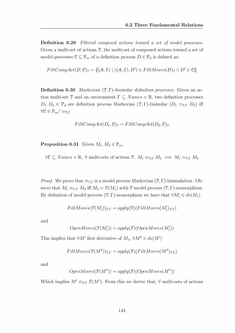
6.2 Three Fundamental Relations
Definition 6.29 Filtered composed actions toward a set of model processes.
Given a multi-set of actions T, the multi-set of composed actions toward a set of
model processes C ⊆ Pm of a definition process D ∈ Pd is defined as:
FiltCompAct(D,C)T = {|(A,E) | ((A,E), D′) ∈ FiltMoves(D)T ∧D′ ∈ C|}
Definition 6.30 Markovian (T,Γ)-bisimilar definition processes. Given an ac-
tion multi-set T and an environment Γ ⊆ Names × R, two definition processes
D1, D2 ∈ Pd are definition process Markovian (T,Γ)-bisimilar (D1 'T,Γ D2) iff
∀C ∈ Pm/ 'T,Γ
FiltCompAct(D1,C)T = FiltCompAct(D2,C)T
Proposition 6.31 Given M1,M2 ∈ Pm,
∀Γ ⊆ Names× R, ∀ multi-sets of actions T, M1 ≡T,Γ M2 =⇒ M1 'T,Γ M2
Proof. We prove that ≡T,Γ is a model process Markovian (T,Γ)-bisimulation. Ob-
serve that M1 ≡T,Γ M2 iff M2 = F(M1) with F model process (T,Γ)-isomorphism.
By definition of model process (T,Γ)-isomorphism we have that ∀M ′1 ∈ ds(M1)
FiltMoves(F(M ′1))T,Γ = apply(F)(FiltMoves(M ′
1)T,Γ)
and
OpenMoves(F(M ′1)) = apply(F)(OpenMoves(M ′
1))
This implies that ∀M ′ first derivative of M1, ∀M ′′ ∈ ds(M ′)
FiltMoves(F(M ′′))T,Γ = apply(F)(FiltMoves(M ′′)T,Γ)
and
OpenMoves(F(M ′′)) = apply(F)(OpenMoves(M ′′))
Which implies M ′ ≡T,Γ F(M ′). From this we derive that, ∀ multi-sets of actions
143
6.2 Three Fundamental Relations
A and E and ∀C ∈ Pm/ ≡T,Γ
νT,Γ(M1,A,E,C) =∑M ′∈C
µT,Γ(M1,A,H,M′) =
∑M ′∈C
µT,Γ(F(M1),A,H,F(M ′))
=∑M ′∈C
µT,Γ(M2,A,H,M′) = νT,Γ(M2,A,H,C)
and
OpenAct(M1,C) = OpenAct(M2,C)
This is possible because M ′ and F(M ′) are (T,Γ)-isomorphic and belong to the
same equivalence class C ∈ Pm/ ≡T,Γ.
Proposition 6.32 Given D1, D2 ∈ Pd,
∀Γ ⊆ Names× R, ∀ multi sets of actions T, D1 ≡T,Γ D2 =⇒ D1 'T,Γ D2
Proof. Given arbitrary Γ ⊆ Names × R and T ⊆ Actions, D1 ≡T,Γ D2 implies
there exists a bijective function F : ds(D1) → ds(D2) such that ∀A ∈ ds(D1),
A ≡T,Γ F(A) and
FiltMoves(D2)T = apply(F)(FiltMoves(D1)T)
We know from Proposition 6.31 that A ≡T,Γ F(A) implies A 'T,Γ F(A). Thus,
A and F(A) are in the same equivalence class C ∈ Pm/ 'T,Γ. This implies
∀C ∈ Pm/ 'T,Γ
FiltCompAct(D1,C)T = FiltCompAct(D2,C)T
Proposition 6.33 Equational laws for Markovian (T,Γ)-bisimilar sPAH pro-
cesses. Because of Propositions 6.31 and 6.32, the equational laws for (T,Γ)-
isomorphic sPAH processes hold as equational laws for Markovian (T,Γ)-bisimilar
sPAH processes.
144
6.2 Three Fundamental Relations
Proposition 6.34 Markovian (T,Γ)-bisimulation as a Congruence. If P1, P2 ∈ Psuch that P1 'T,Γ P2, then
1. A[E].P1 'T,Γ A[E].P2, with P1, P2 agents
2. P1 +Q 'T,Γ P2 +Q, with P1, P2, Q ∈ Pd
3. P1 BCLQ 'T,Γ P2 BC
LQ, with P1, P2, Q ∈ Pm
4. P1 BC
LQ 'T,Γ P2 BC
LQ, with P1, P2, Q ∈ Pm
Proof. Proof of each case:
1. We know by assumption that P1 'T,Γ P2. This implies P1, P2 ∈ C, with
C ∈ Pm/ 'T,Γ. Now, FiltMoves(A[E].P1)T = {|(((A \ T),E), P1)|} and
FiltMoves(A[E].P2)T = {|(((A \ T),E), P2)|}. This implies ∀C ∈ Pm/ 'T,Γ
FiltCompAct(A[E].P1,C)T = FiltCompAct(A[E].P2,C)T
2. P1 + Q and P2 + Q are definition processes. Because P1 'T,Γ P2 we have
that ∀C ∈ Pm/ 'T,Γ
FiltCompAct(P1 +Q,C)T =
FiltCompAct(P1,C)T ] FiltCompAct(Q,C)T =
FiltCompAct(P2,C)T ] FiltCompAct(Q,C)T =
FiltCompAct(P2 +Q,C)T
3. We prove that the relation R = {(P1 BCLQ,P2 BC
LQ) | P1 'T,Γ P2} is a
Markovian (T,Γ)-bisimulation. We consider four cases:
(a) ∀r ∈ R, (A,E, r) 6∈ FiltAct(P1 BCLQ)T,Γ. This implies that ∀r ∈
R, (A,E, r) 6∈ FiltAct(P2 BCLQ)T,Γ, because a filtered activity for
P BCLQ is either a filtered activity of P , a filtered activity of Q or
it is derived from a closed activity which is the synchronisation of an
open activity from P and one from Q and P1 'T,Γ P2 implies
145
6.2 Three Fundamental Relations
• ∀r ∈ R, (A,E, r) 6∈ FiltAct(P1)T,Γ ⇔ ∀r ∈ R, (A,E, r) 6∈FiltAct(P2)T,Γ;
• ∀C ∈ Pm/ 'T,Γ OpenAct(P1,C) = OpenAct(P2,C).
It follows that ∀C ∈ Pm/ 'T,Γ
νT,Γ(P1 BCLQ,A,E, C) = νT,Γ(P2 BC
LQ,A,E, C) = 0
(b) ∃r ∈ R, ((A,E, r), P ′1 BCL Q) ∈ FiltMoves(P1 BCLQ)T,Γ. Recall that
P1 'T,Γ P2 implies
∃r ∈ R, ((A,E, r), P ′1) ∈ FiltMoves(P1)T,Γ ⇔
∃r′ ∈ R, ((A,E, r′), P ′2) ∈ FiltMoves(P2)T,Γ
with P ′1 'T,Γ P′2, because νT,Γ(P1,A,E, [P
′1]'T,Γ
) = νT,Γ(P2,A,E, [P′1]'T,Γ
).
It follows that
νT,Γ(P1 BCLQ,A,E, [P ′1 BCL Q]R) = νT,Γ(P1,A,E, [P
′1]'T,Γ
) =
νT,Γ(P2,A,E, [P′1]'T,Γ
) = νT,Γ(P2 BCLQ,A,E, [P ′2 BCL Q]R)
It is also important to recall that if an activity is filtered then it is
derived from a closed activity, which in turn means that no further
synchronisation is possible via BCL
. This is because of Condition 3 in
Definition 5.12.
(c) ∃r ∈ R, ((A,E, r), P1 BCLQ′) ∈ FiltMoves(P1 BC
LQ)T,Γ. It follows
that
νT,Γ(P1 BCLQ,A,E, [P1 BC
LQ′]R) = νT,Γ(Q,A,E, [Q′]'T,Γ
) =
= νT,Γ(P2 BCLQ,A,E, [P1 BC
LQ′]R)
Because P1 'T,Γ P2 and so P2 BCLQ′ ∈ [P1 BC
LQ′]R.
(d) ∃r ∈ R, ((A,E, r), P ′1 BCL Q′) ∈ FiltMoves(P1 BCLQ)T,Γ. The filtered
move ((A,E, r), P ′1 BCL Q′) must be the result of a synchronisation be-
tween an open move from P1 and an open move from Q. In par-
ticular, it must be that ∃(A1[E1],Γ1) ∈ OpenAct(P1, [P′1]'T,Γ
) and
146
6.2 Three Fundamental Relations
∃(A2[E2],Γ2) ∈ OpenAct(Q, [Q′]'T,Γ) such that:
• B = A1 ∪A2, E = E1 ] E2 and Γ′ = Γ1 ∪ Γ2;
• (B[E],Γ′) ∈ ClosedAct(P1 BCLQ);
• {a} = activeActions(B)F;
• {|(A,E, k)|} = filterActivities(T)(rateActivities(Γ)({|(B[E],Γ′)|}));
• r = k/π(ClosedAct(P1 BCLQ), (a,Γ′)).
Moreover, from P1 'T,Γ P2 we have that
((A1[E1],Γ1), P ′1) ∈ OpenMoves(P1)⇔
((A1[E1],Γ1), P ′2) ∈ OpenMoves(P2)
with P ′1 'T,Γ P′2, becauseOpenAct(P1, [P
′1]'T,Γ
) = OpenAct(P2, [P′1]'T,Γ
).
It follows that
νT,Γ(P1 BCLQ,A,E, [P ′1 BCL Q′]R) = νT,Γ(P2 BC
LQ,A,E, [P ′1 BCL Q′]R)
where P ′2 BCL Q′ ∈ [P ′1 BCL Q′]R.
4. We prove that the relation R = {(P1 BC
LQ,P2 BC
LQ) | P1 'T,Γ P2} is a
Markovian (T,Γ)-bisimulation. We consider four cases:
(a) ∀r ∈ R, (A,E, r) 6∈ FiltAct(P1 BC
LQ)T,Γ. This implies that ∀r ∈
R, (A,E, r) 6∈ FiltAct(P2 BC
LQ)T,Γ, because a filtered activity for
P BC
LQ is either a filtered activity of P , a filtered activity of Q or
it is derived from a synchronisation of a filtered activity from P and
an open activity from Q or a filtered activity from Q and an open
activity from P and P1 'T,Γ P2 implies
• ∀r ∈ R, (A,E, r) 6∈ FiltAct(P1)T,Γ ⇔ ∀r ∈ R, (A,E, r) 6∈FiltAct(P2)T,Γ;
• ∀C ∈ Pm/ 'T,Γ OpenAct(P1,C) = OpenAct(P2,C).
It follows that ∀C ∈ Pm/ 'T,Γ
νT,Γ(P1 BC
LQ,A,E, C) = νT,Γ(P2 BC
LQ,A,E, C) = 0
147
6.2 Three Fundamental Relations
(b) ∃r ∈ R, ((A,E, r), P ′1 BC
LQ) ∈ FiltMoves(P1 BC
LQ)T,Γ. This implies
that ((A,E, r), P ′1) ∈ FiltMoves(P1)T,Γ and that ¬(∃B,F,Γ′, Q′ s.t.
((B[F],Γ′), Q′) ∈Moves(Q) ∧B ⊆ E ∩ L). Moreover,
∃r ∈ R, ((A,E, r), P ′1) ∈ FiltMoves(P1)T,Γ ⇔
∃r′ ∈ R, ((A,E, r′), P ′2) ∈ FiltMoves(P2)T,Γ
with P ′1 'T,Γ P′2, because νT,Γ(P1,A,E, [P
′1]'T,Γ
) = νT,Γ(P2,A,E, [P′1]'T,Γ
).
It follows that
νT,Γ(P1 BC
LQ,A,E, [P ′1 BC
LQ]R) = νT,Γ(P1,A,E, [P
′1]'T,Γ
) =
νT,Γ(P2,A,E, [P′1]'T,Γ
) = νT,Γ(P2 BC
LQ,A,E, [P ′1 BC
LQ]R)
(c) ∃r ∈ R, ((A,E, r), P1 BC
LQ′) ∈ FiltMoves(P1 BC
LQ)T,Γ. This implies
that ((A,E, r), Q′) ∈ FiltMoves(Q)T,Γ and that ¬(∃B,F,Γ′, P ′1 s.t.
((B[F],Γ′), P ′1) ∈Moves(P1) ∧B ⊆ E ∩ L).
Because ∀C ∈ Pm/ 'T,Γ, OpenAct(P1,C) = OpenAct(P2,C) then
νT,Γ(P1 BC
LQ,A,E, [P1 BC
LQ′]R) = νT,Γ(Q,A,E, [Q′]'T,Γ
) =
νT,Γ(P2 BC
LQ,A,E, [P1 BC
LQ′]R)
(d) ∃r ∈ R, ((A,E, r), P ′1 BC
LQ′) ∈ FiltMoves(P1 BC
LQ)T,Γ. This implies
that filtered move ((A,E, r), P ′1 BC
LQ′) is the result of the synchronisa-
tion of a filtered move of P1 and an open move of Q or the synchroni-
sation of a filtered move from Q and an open move from P1.
In this case we have
νT,Γ(P1 BC
LQ,A,E, [P ′1 BC
LQ′]R) =∑
i∈I
νT,Γ(P1,Ai,Ei, [P′1]'T,Γ
) +∑j∈J
νT,Γ(Q,Aj,EJ , [Q′]'T,Γ
) =
∑i∈I
νT,Γ(P2,Ai,Ei, [P′1]'T,Γ
) +∑j∈J
νT,Γ(Q,Aj,EJ , [Q′]'T,Γ
) =
νT,Γ(P2 BC
LQ,A,E, [P ′1 BC
LQ′]R)
148
6.2 Three Fundamental Relations
Once again because
∃r ∈ R, ((A,E, r), P ′1) ∈ FiltMoves(P1)T,Γ ⇔
∃r′ ∈ R, ((A,E, r′), P ′2) ∈ FiltMoves(P2)T,Γ
with P ′1 'T,Γ P′2, because νT,Γ(P1,A,E, [P
′1]'T,Γ
) = νT,Γ(P2,A,E, [P′1]'T,Γ
).
Moreover
• i ∈ I if and only if ∃B,F,Γ′, Q′ s.t. ((B[F],Γ′), Q′) ∈ Moves(Q)
and B ⊆ Ei ∩ L and A = Ai ∪ (B ∩ T) and E = (Ei \ B) ] F
and ¬(∃B′,F′,Γ′′, Q′′ s.t. ((B′[F′],Γ′′), Q′′) ∈Moves(Q) and B′ ⊆Ei ∩ L and |B′| > |B|);
• j ∈ J if and only if ∃B,F,Γ′, P ′1 s.t. ((B[F],Γ′), P ′1) ∈Moves(P )
and B ⊆ Ej ∩ L and A = Aj ∪ (B ∩ T) and E = (Ej \ B) ]F and ¬(∃B′,F′,Γ′′, Q′′ s.t. ((B′[F′],Γ′′), P ′′1 ) ∈ Moves(P1) and
B′ ⊆ Ej ∩ L and |B′| > |B|).
We also use the fact that ∀C ∈ Pm/ 'T,Γ, OpenAct(P1,C) = OpenAct(P2,C).
Since we proved all four cases, the result holds.
6.2.3 Practical Use of the Relations
The three relations defined in this chapter represent the foundation of the theory
of relations on sPAH. They are the strongest relations one can define, consider-
ing in turn the structure of the model (isomorphism), filtering of activities (T-
isomorphism) and timing and probability of actions (Markovian T-bisimulation).
In a case study in Section 7.2, we will illustrate how the fact that Markovian
T-bisimulation is a congruence can be exploited to extend the equality of parts
of two model to the entire models.
As it can be expected from such strong relations, they may be too strong for
many biological applications, but other relations can be defined using these as a
starting point. In particular, in biology one is often interested in knowing whether
two systems are almost rather than exactly the same, and possibly to which extent
they are similar. We will discuss more about this in the last chapter, in the future
work section.
149
6.3 Summary
6.3 Summary
In this chapter we discussed the idea of relating quantitative multi-scale models of
biological systems at a specified scale using process algebra with hooks. After in-
troducing filtering as a procedure that can be used to focus on a specified scale, we
defined three relations on process algebra with hooks models: isomorphism (≡),
T-isomorphism (≡T) and Markovian T-bisimulation ('T). In turn, isomorphism
relates processes that produce isomorphic derivation graphs, T-isomorphism re-
lates processes that produce derivation graphs that are isomorphic after rating
and filtering and Markovian T-bisimulation relates processes that perform the
same filtered actions with the same probability at the same time. Fundamental
properties of the relations, such as equational laws and congruence are also pro-
vided. Although these relations are probably too strong to be of practical use
in the biological setting, they nevertheless can be considered the fundamental
relations, the starting point from which other relations can be defined.
150
Chapter 7
Case Study
In this chapter we illustrate how process algebra with hooks can be employed to
model complex multi-scale scenarios. Before presenting the models we introduce
a parametric version of stochastic process algebra with hooks (Section 7.1); this is
a minor extension, which does not affect the theory of earlier chapters, but makes
model descriptions more compact. The two scenarios we model in this chapter
are: a typical problem of pattern formation (Section 7.2), and a multi-scale model
of tissue growth (Section 7.3). We perform analysis using an interpreter and
simulator developed for parametric stochastic process algebra with hooks.
7.1 Parametric Stochastic Process Algebra with
Hooks
In this section we introduce the syntax of a parametric version of sPAH. We
augment sPAH defined in Section 5.2 with parametrised processes and actions, in
analogy with our definition of pSPA in Section 3.3, and we obtain a parametric
stochastic process algebra with hooks (psPAH). The syntax of psPAH is as follows:
D ::= nil | L′[L′′].A(exp, . . . , exp) | D +D | if bexp then D else D
M ::= A(k, . . . , k) |M BCLM |M BC
LM
exp ::= k | i | exp+ exp | exp− exp | exp/exp | exp ∗ exp
bexp ::= exp = exp | exp < exp | bexp ∧ bexp |
bexp ∨ bexp | ¬bexp | true | false
151
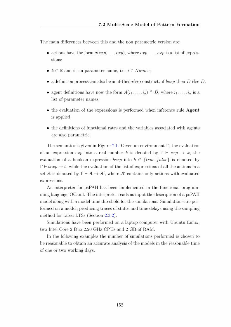
7.2 Multi-Scale Model of Pattern Formation
The main differences between this and the non parametric version are:
• actions have the form a(exp, . . . , exp), where exp, . . . , exp is a list of expres-
sions;
• k ∈ R and i is a parameter name, i.e. i ∈ Names;
• a definition process can also be an if-then-else construct: if bexp then D else D;
• agent definitions have now the form A(i1, . . . , in) , D, where i1, . . . , in is a
list of parameter names;
• the evaluation of the expressions is performed when inference rule Agent
is applied;
• the definitions of functional rates and the variables associated with agents
are also parametric.
The semantics is given in Figure 7.1. Given an environment Γ, the evaluation
of an expression exp into a real number k is denoted by Γ ` exp → k, the
evaluation of a boolean expression bexp into b ∈ {true, false} is denoted by
Γ ` bexp→ b, while the evaluation of the list of expressions of all the actions in a
set A is denoted by Γ ` A → A′, where A′ contains only actions with evaluated
expressions.
An interpreter for psPAH has been implemented in the functional program-
ming language OCaml. The interpreter reads as input the description of a psPAH
model along with a model time threshold for the simulations. Simulations are per-
formed on a model, producing traces of states and time delays using the sampling
method for rated LTSs (Section 2.3.2).
Simulations have been performed on a laptop computer with Ubuntu Linux,
two Intel Core 2 Duo 2.20 GHz CPUs and 2 GB of RAM.
In the following examples the number of simulations performed is chosen to
be reasonable to obtain an accurate analysis of the models in the reasonable time
of one or two working days.
152
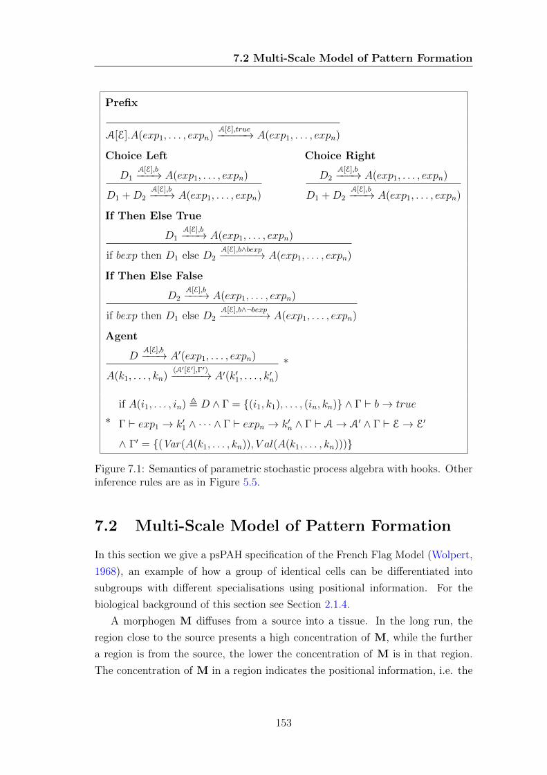
7.2 Multi-Scale Model of Pattern Formation
Prefix
A[E].A(exp1, . . . , expn)A[E],true−−−−−→ A(exp1, . . . , expn)
Choice Left Choice Right
D1A[E],b−−−→ A(exp1, . . . , expn)
D1 +D2A[E],b−−−→ A(exp1, . . . , expn)
D2A[E],b−−−→ A(exp1, . . . , expn)
D1 +D2A[E],b−−−→ A(exp1, . . . , expn)
If Then Else True
D1A[E],b−−−→ A(exp1, . . . , expn)
if bexp then D1 else D2A[E],b∧bexp−−−−−−→ A(exp1, . . . , expn)
If Then Else False
D2A[E],b−−−→ A(exp1, . . . , expn)
if bexp then D1 else D2A[E],b∧¬bexp−−−−−−−→ A(exp1, . . . , expn)
Agent
DA[E],b−−−→ A′(exp1, . . . , expn)
A(k1, . . . , kn)(A′[E′],Γ′)−−−−−→ A′(k′1, . . . , k
′n)
*
*
if A(i1, . . . , in) , D ∧ Γ = {(i1, k1), . . . , (in, kn)} ∧ Γ ` b→ true
Γ ` exp1 → k′1 ∧ · · · ∧ Γ ` expn → k′n ∧ Γ ` A→ A′ ∧ Γ ` E→ E′
∧ Γ′ = {(Var(A(k1, . . . , kn)), V al(A(k1, . . . , kn)))}
Figure 7.1: Semantics of parametric stochastic process algebra with hooks. Otherinference rules are as in Figure 5.5.
7.2 Multi-Scale Model of Pattern Formation
In this section we give a psPAH specification of the French Flag Model (Wolpert,
1968), an example of how a group of identical cells can be differentiated into
subgroups with different specialisations using positional information. For the
biological background of this section see Section 2.1.4.
A morphogen M diffuses from a source into a tissue. In the long run, the
region close to the source presents a high concentration of M, while the further
a region is from the source, the lower the concentration of M is in that region.
The concentration of M in a region indicates the positional information, i.e. the
153
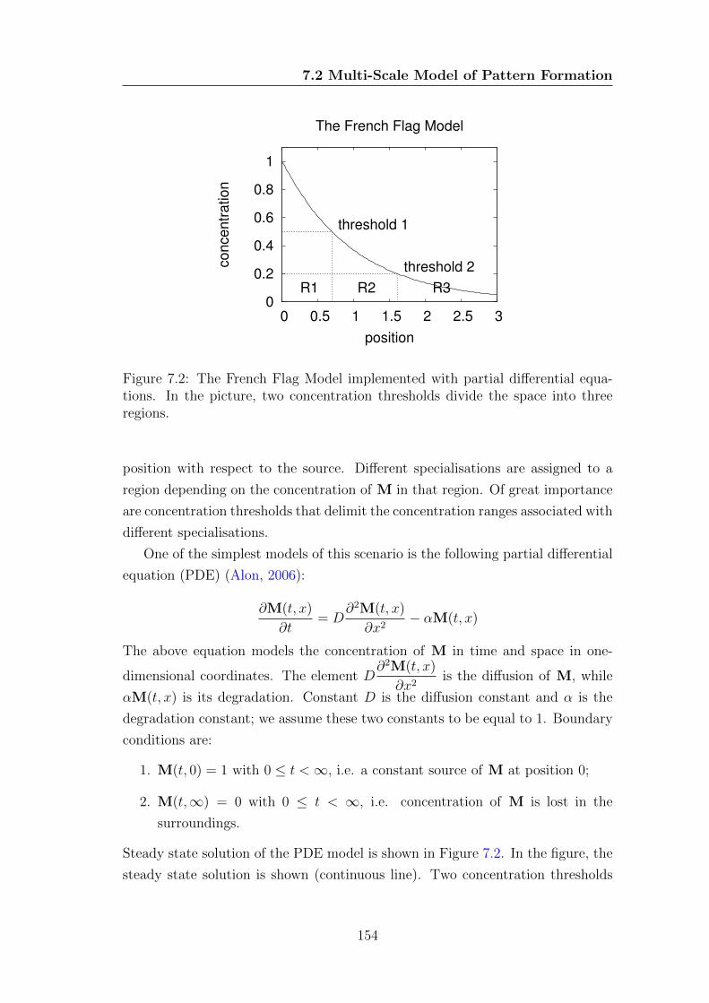
7.2 Multi-Scale Model of Pattern Formation
0
0.2
0.4
0.6
0.8
1
0 0.5 1 1.5 2 2.5 3
concentr
ation
position
The French Flag Model
threshold 1
threshold 2
R1 R2 R3
Figure 7.2: The French Flag Model implemented with partial differential equa-tions. In the picture, two concentration thresholds divide the space into threeregions.
position with respect to the source. Different specialisations are assigned to a
region depending on the concentration of M in that region. Of great importance
are concentration thresholds that delimit the concentration ranges associated with
different specialisations.
One of the simplest models of this scenario is the following partial differential
equation (PDE) (Alon, 2006):
∂M(t, x)
∂t= D
∂2M(t, x)
∂x2− αM(t, x)
The above equation models the concentration of M in time and space in one-
dimensional coordinates. The element D∂2M(t, x)
∂x2is the diffusion of M, while
αM(t, x) is its degradation. Constant D is the diffusion constant and α is the
degradation constant; we assume these two constants to be equal to 1. Boundary
conditions are:
1. M(t, 0) = 1 with 0 ≤ t <∞, i.e. a constant source of M at position 0;
2. M(t,∞) = 0 with 0 ≤ t < ∞, i.e. concentration of M is lost in the
surroundings.
Steady state solution of the PDE model is shown in Figure 7.2. In the figure, the
steady state solution is shown (continuous line). Two concentration thresholds
154
7.2 Multi-Scale Model of Pattern Formation
Figure 7.3: Discretisation of the space of the French Flag Model into 20 regions.The variable M(i) indicates the concentration of M at region 1.
(at 0.2 and 0.5, dotted lines) divide the area in three regions (R1, R2 and R3).
Each of these regions are characterised by a different specialisation.
We propose now a representation of the PDE model in psPAH. Because the
PDE model is continuous in the concentration of M and in space, while psPAH
uses a discrete representation of these quantities, we provide a discretisation. We
assume 20 levels for the concentration of M (parameter maxLevels = 20), with
maximum concentration equal to 1 and concentration of each level equal to h =
1/20 = 0.05, and we assume 20 regions of space (parameter regions = 20), with
total length equal to 3 and length of each region equal to deltaX = 3/20 = 0, 15.
The spatial discretisation is illustrated in Figure 7.3.
In order to represent the two boundary conditions we have:
• the left most region presents a constant concentration level of 20, which
guarantees that concentration flows continuously from the left;
• the right most region presents a constant concentration level equal to 0,
which implies that this region absorbs concentration levels.
We define agent M(i, w) (Figure 7.4) to indicate that morphogen M in region
i presents concentration level w. Actions t(i, j) represent transport of M from
region i to region j, while actions deg(i) represent degradation of M in region i.
We model specialisation of regions explicitly as follows. Two thresholds are
considered: one between 4 and 5 concentration levels and the other between 10
and 11. Whenever a concentration threshold is crossed in a region, the speciali-
sation of the region changes. The presence of two thresholds implies that three
specialisations are possible, corresponding to high, medium and low concentration
ranges of M. In addition, we consider that regions of tissue can commit perma-
nently to a specialisation, if the concentration of M in those regions stays at a
certain concentration range long enough. A commitment means that the cells in
the committed region have memorised their positional information and further
155
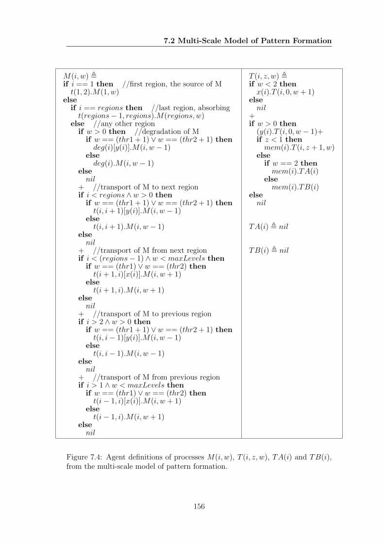
7.2 Multi-Scale Model of Pattern Formation
M(i, w) ,if i == 1 then //first region, the source of Mt(1, 2).M(1, w)
elseif i == regions then //last region, absorbingt(regions− 1, regions).M(regions, w)
else //any other regionif w > 0 then //degradation of M
if w == (thr1 + 1) ∨ w == (thr2 + 1) thendeg(i)[y(i)].M(i, w − 1)
elsedeg(i).M(i, w − 1)
elsenil
+ //transport of M to next regionif i < regions ∧ w > 0 then
if w == (thr1 + 1) ∨ w == (thr2 + 1) thent(i, i+ 1)[y(i)].M(i, w − 1)
elset(i, i+ 1).M(i, w − 1)
elsenil
+ //transport of M from next regionif i < (regions− 1) ∧ w < maxLevels then
if w == (thr1) ∨ w == (thr2) thent(i+ 1, i)[x(i)].M(i, w + 1)
elset(i+ 1, i).M(i, w + 1)
elsenil
+ //transport of M to previous regionif i > 2 ∧ w > 0 then
if w == (thr1 + 1) ∨ w == (thr2 + 1) thent(i, i− 1)[y(i)].M(i, w − 1)
elset(i, i− 1).M(i, w − 1)
elsenil
+ //transport of M from previous regionif i > 1 ∧ w < maxLevels then
if w == (thr1) ∨ w == (thr2) thent(i− 1, i)[x(i)].M(i, w + 1)
elset(i− 1, i).M(i, w + 1)
elsenil
T (i, z, w) ,if w < 2 thenx(i).T (i, 0, w + 1)
elsenil
+if w > 0 then
(y(i).T (i, 0, w − 1)+if z < 1 thenmem(i).T (i, z + 1, w)
elseif w == 2 thenmem(i).TA(i)
elsemem(i).TB(i)
elsenil
TA(i) , nil
TB(i) , nil
Figure 7.4: Agent definitions of processes M(i, w), T (i, z, w), TA(i) and TB(i),from the multi-scale model of pattern formation.
156
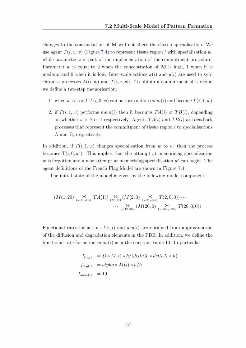
7.2 Multi-Scale Model of Pattern Formation
changes to the concentration of M will not affect the chosen specialisation. We
use agent T (i, z, w) (Figure 7.4) to represent tissue region i with specialisation w,
while parameter z is part of the implementation of the commitment procedure.
Parameter w is equal to 2 when the concentration of M is high, 1 when it is
medium and 0 when it is low. Inter-scale actions x(i) and y(i) are used to syn-
chronise processes M(i, w) and T (i, z, w). To obtain a commitment of a region
we define a two-step memorisation:
1. when w is 1 or 2, T (i, 0, w) can perform actionmem(i) and become T (i, 1, w);
2. if T (i, 1, w) performs mem(i) then it becomes TA(i) or TB(i), depending
on whether w is 2 or 1 respectively. Agents TA(i) and TB(i) are deadlock
processes that represent the commitment of tissue region i to specialisations
A and B, respectively.
In addition, if T (i, 1, w) changes specialisation from w to w′ then the process
becomes T (i, 0, w′). This implies that the attempt at memorising specialisation
w is forgotten and a new attempt at memorising specialisation w′ can begin. The
agent definitions of the French Flag Model are shown in Figure 7.4.
The initial state of the model is given by the following model component:
(M(1, 20) BC
{|x(1),y(1)|}TA(1)) BC
{|t(1,2)|}(M(2, 0) BC
{|x(2),y(2)|}T (2, 0, 0)) · · ·
· · · BC{|t(19,20)|}
(M(20, 0) BC
{|x(20),y(20)|}T (20, 0, 0))
Functional rates for actions t(i, j) and deg(i) are obtained from approximation
of the diffusion and degradation elements in the PDE. In addition, we define the
functional rate for action mem(i) as a the constant value 10. In particular:
ft(i,j) = D ∗M(i) ∗ h/(deltaX ∗ deltaX ∗ h)
fdeg(i) = alpha ∗M(i) ∗ h/h
fmem(i) = 10
157
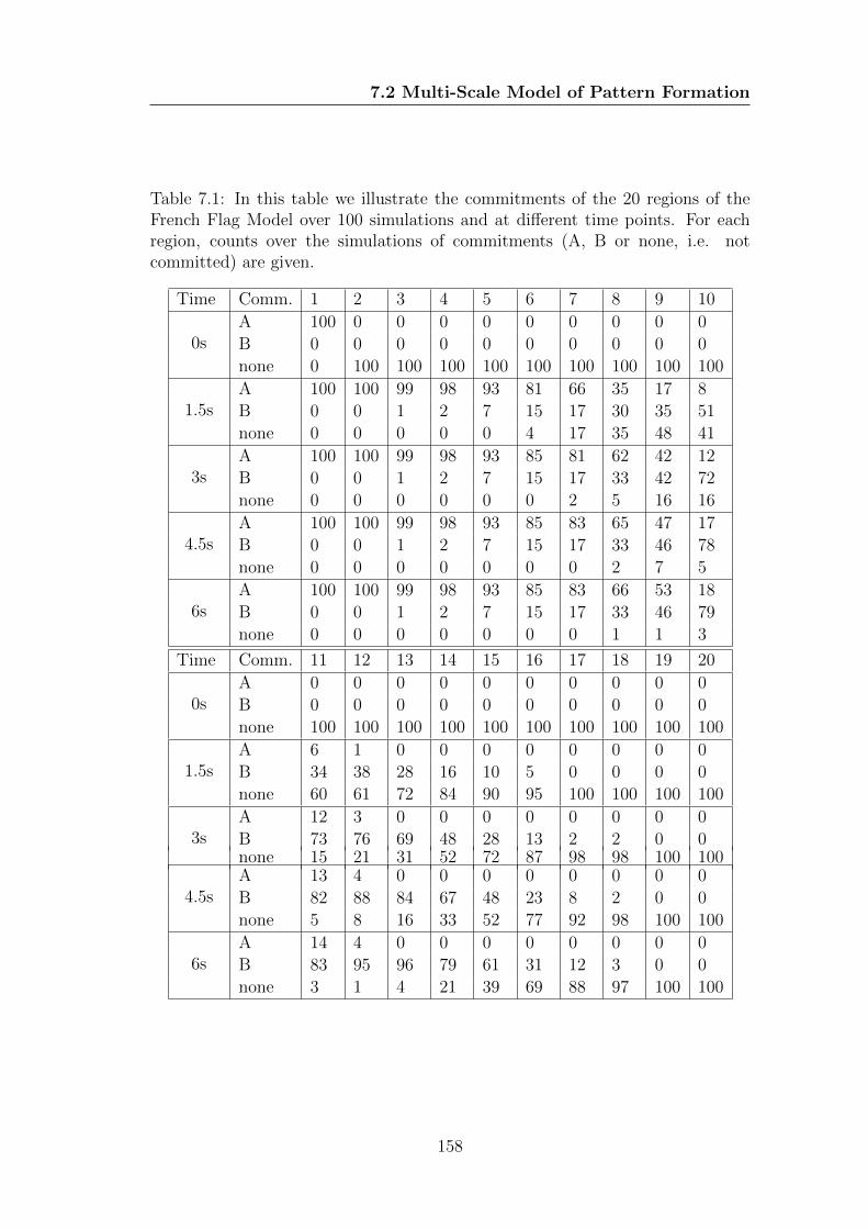
7.2 Multi-Scale Model of Pattern Formation
Table 7.1: In this table we illustrate the commitments of the 20 regions of theFrench Flag Model over 100 simulations and at different time points. For eachregion, counts over the simulations of commitments (A, B or none, i.e. notcommitted) are given.
Time Comm. 1 2 3 4 5 6 7 8 9 10
0sA 100 0 0 0 0 0 0 0 0 0
B 0 0 0 0 0 0 0 0 0 0
none 0 100 100 100 100 100 100 100 100 100
1.5sA 100 100 99 98 93 81 66 35 17 8
B 0 0 1 2 7 15 17 30 35 51
none 0 0 0 0 0 4 17 35 48 41
3sA 100 100 99 98 93 85 81 62 42 12
B 0 0 1 2 7 15 17 33 42 72
none 0 0 0 0 0 0 2 5 16 16
4.5sA 100 100 99 98 93 85 83 65 47 17
B 0 0 1 2 7 15 17 33 46 78
none 0 0 0 0 0 0 0 2 7 5
6sA 100 100 99 98 93 85 83 66 53 18
B 0 0 1 2 7 15 17 33 46 79
none 0 0 0 0 0 0 0 1 1 3
Time Comm. 11 12 13 14 15 16 17 18 19 20
0sA 0 0 0 0 0 0 0 0 0 0
B 0 0 0 0 0 0 0 0 0 0
none 100 100 100 100 100 100 100 100 100 100
1.5sA 6 1 0 0 0 0 0 0 0 0
B 34 38 28 16 10 5 0 0 0 0
none 60 61 72 84 90 95 100 100 100 100
3sA 12 3 0 0 0 0 0 0 0 0
B 73 76 69 48 28 13 2 2 0 0none 15 21 31 52 72 87 98 98 100 100
4.5sA 13 4 0 0 0 0 0 0 0 0
B 82 88 84 67 48 23 8 2 0 0
none 5 8 16 33 52 77 92 98 100 100
6sA 14 4 0 0 0 0 0 0 0 0
B 83 95 96 79 61 31 12 3 0 0
none 3 1 4 21 39 69 88 97 100 100
158
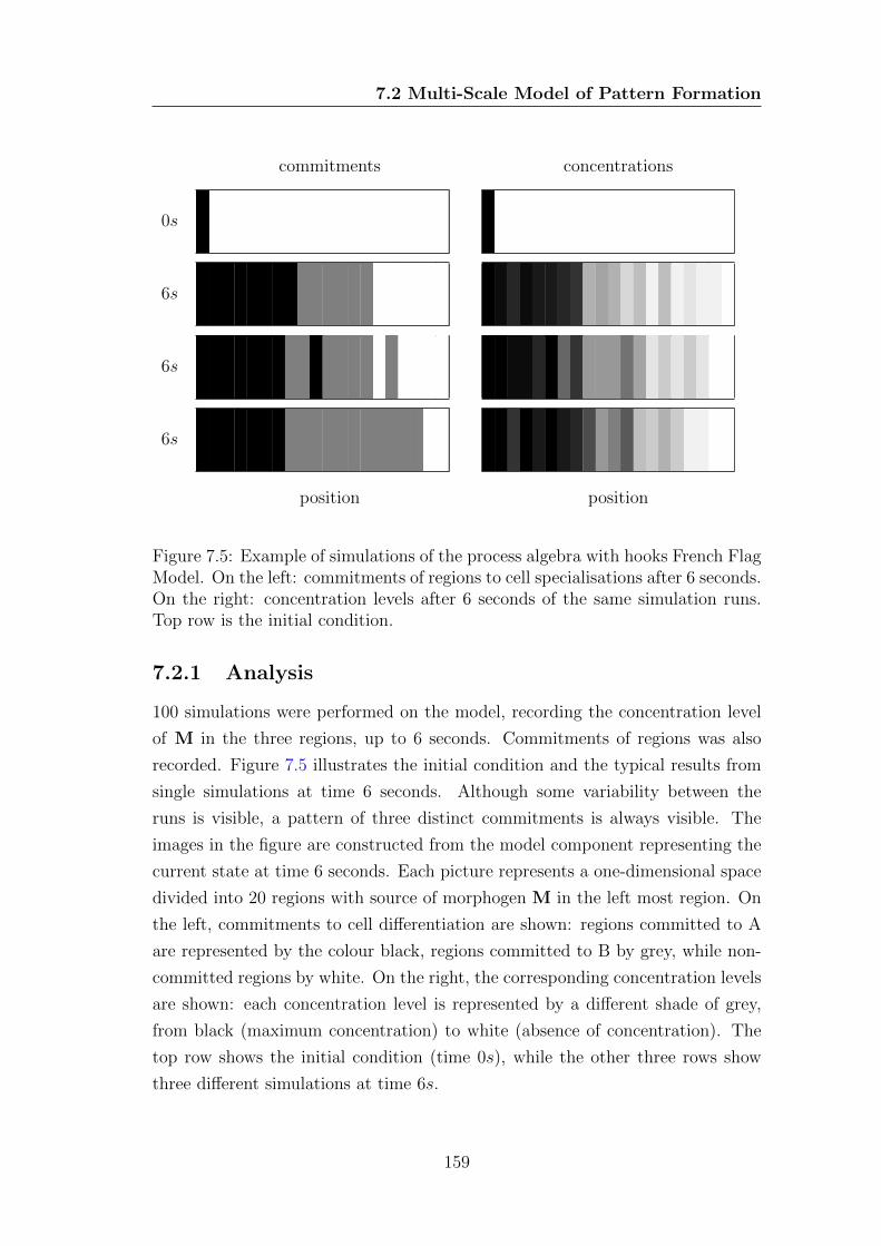
7.2 Multi-Scale Model of Pattern Formation
commitments concentrations
0s
6s
6s
6s
position position
Figure 7.5: Example of simulations of the process algebra with hooks French FlagModel. On the left: commitments of regions to cell specialisations after 6 seconds.On the right: concentration levels after 6 seconds of the same simulation runs.Top row is the initial condition.
7.2.1 Analysis
100 simulations were performed on the model, recording the concentration level
of M in the three regions, up to 6 seconds. Commitments of regions was also
recorded. Figure 7.5 illustrates the initial condition and the typical results from
single simulations at time 6 seconds. Although some variability between the
runs is visible, a pattern of three distinct commitments is always visible. The
images in the figure are constructed from the model component representing the
current state at time 6 seconds. Each picture represents a one-dimensional space
divided into 20 regions with source of morphogen M in the left most region. On
the left, commitments to cell differentiation are shown: regions committed to A
are represented by the colour black, regions committed to B by grey, while non-
committed regions by white. On the right, the corresponding concentration levels
are shown: each concentration level is represented by a different shade of grey,
from black (maximum concentration) to white (absence of concentration). The
top row shows the initial condition (time 0s), while the other three rows show
three different simulations at time 6s.
159
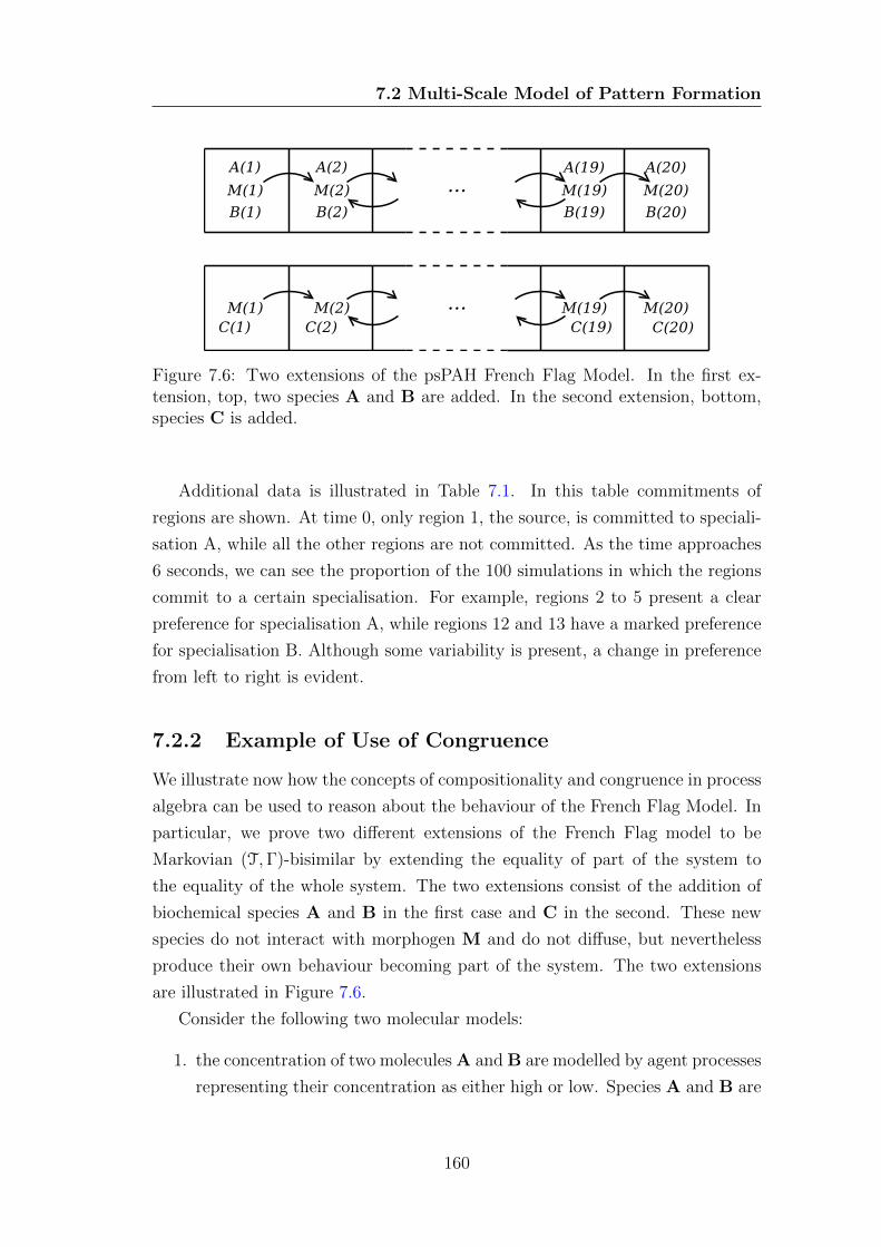
7.2 Multi-Scale Model of Pattern Formation
Figure 7.6: Two extensions of the psPAH French Flag Model. In the first ex-tension, top, two species A and B are added. In the second extension, bottom,species C is added.
Additional data is illustrated in Table 7.1. In this table commitments of
regions are shown. At time 0, only region 1, the source, is committed to speciali-
sation A, while all the other regions are not committed. As the time approaches
6 seconds, we can see the proportion of the 100 simulations in which the regions
commit to a certain specialisation. For example, regions 2 to 5 present a clear
preference for specialisation A, while regions 12 and 13 have a marked preference
for specialisation B. Although some variability is present, a change in preference
from left to right is evident.
7.2.2 Example of Use of Congruence
We illustrate now how the concepts of compositionality and congruence in process
algebra can be used to reason about the behaviour of the French Flag Model. In
particular, we prove two different extensions of the French Flag model to be
Markovian (T,Γ)-bisimilar by extending the equality of part of the system to
the equality of the whole system. The two extensions consist of the addition of
biochemical species A and B in the first case and C in the second. These new
species do not interact with morphogen M and do not diffuse, but nevertheless
produce their own behaviour becoming part of the system. The two extensions
are illustrated in Figure 7.6.
Consider the following two molecular models:
1. the concentration of two molecules A and B are modelled by agent processes
representing their concentration as either high or low. Species A and B are
160
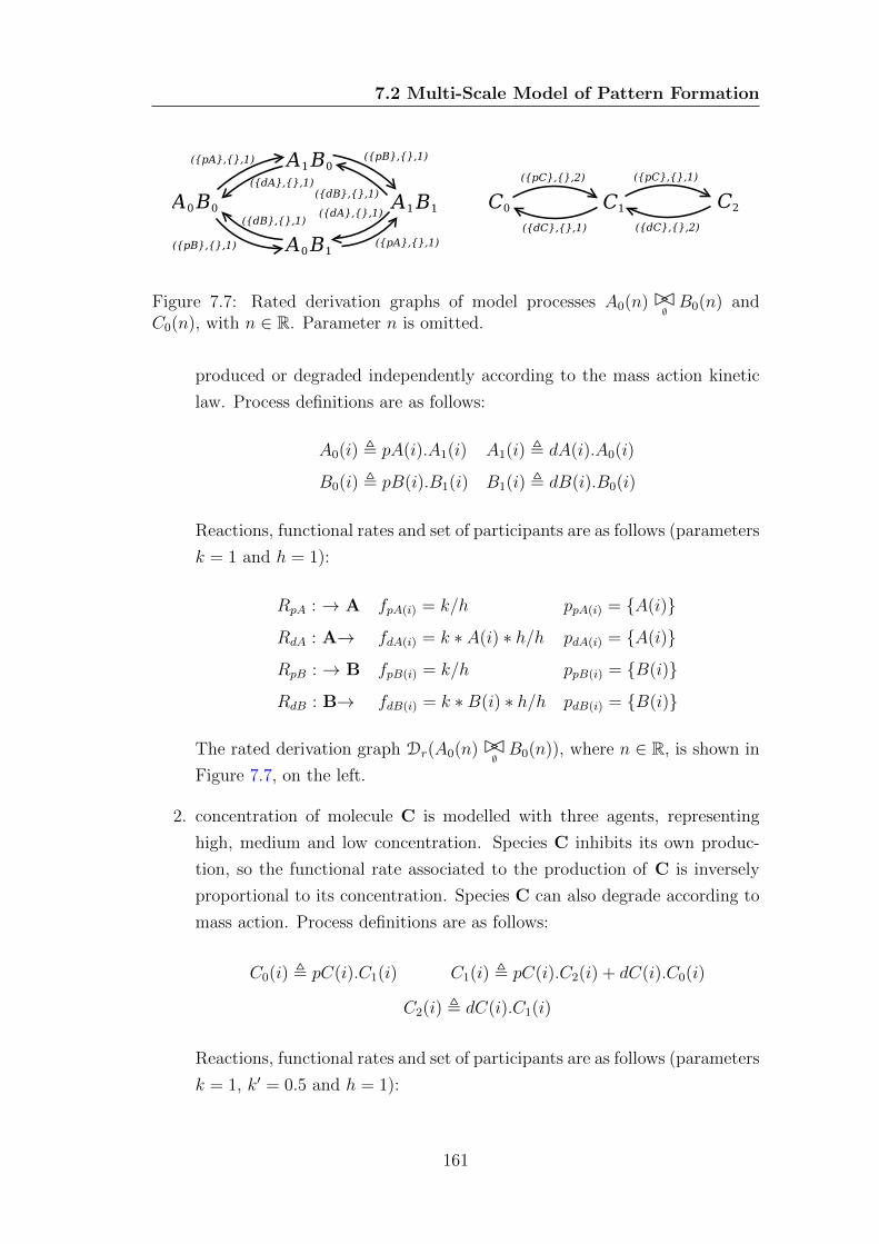
7.2 Multi-Scale Model of Pattern Formation
Figure 7.7: Rated derivation graphs of model processes A0(n)BC∅B0(n) and
C0(n), with n ∈ R. Parameter n is omitted.
produced or degraded independently according to the mass action kinetic
law. Process definitions are as follows:
A0(i) , pA(i).A1(i) A1(i) , dA(i).A0(i)
B0(i) , pB(i).B1(i) B1(i) , dB(i).B0(i)
Reactions, functional rates and set of participants are as follows (parameters
k = 1 and h = 1):
RpA : → A fpA(i) = k/h ppA(i) = {A(i)}
RdA : A→ fdA(i) = k ∗ A(i) ∗ h/h pdA(i) = {A(i)}
RpB : → B fpB(i) = k/h ppB(i) = {B(i)}
RdB : B→ fdB(i) = k ∗B(i) ∗ h/h pdB(i) = {B(i)}
The rated derivation graph Dr(A0(n)BC∅B0(n)), where n ∈ R, is shown in
Figure 7.7, on the left.
2. concentration of molecule C is modelled with three agents, representing
high, medium and low concentration. Species C inhibits its own produc-
tion, so the functional rate associated to the production of C is inversely
proportional to its concentration. Species C can also degrade according to
mass action. Process definitions are as follows:
C0(i) , pC(i).C1(i) C1(i) , pC(i).C2(i) + dC(i).C0(i)
C2(i) , dC(i).C1(i)
Reactions, functional rates and set of participants are as follows (parameters
k = 1, k′ = 0.5 and h = 1):
161
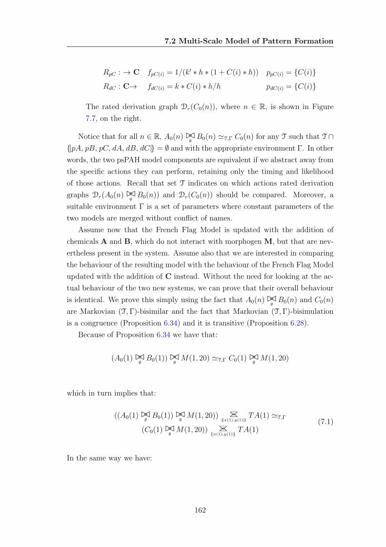
7.2 Multi-Scale Model of Pattern Formation
RpC : → C fpC(i) = 1/(k′ ∗ h ∗ (1 + C(i) ∗ h)) ppC(i) = {C(i)}
RdC : C→ fdC(i) = k ∗ C(i) ∗ h/h pdC(i) = {C(i)}
The rated derivation graph Dr(C0(n)), where n ∈ R, is shown in Figure
7.7, on the right.
Notice that for all n ∈ R, A0(n)BC∅B0(n) 'T,Γ C0(n) for any T such that T ∩
{|pA, pB, pC, dA, dB, dC|} = ∅ and with the appropriate environment Γ. In other
words, the two psPAH model components are equivalent if we abstract away from
the specific actions they can perform, retaining only the timing and likelihood
of those actions. Recall that set T indicates on which actions rated derivation
graphs Dr(A0(n)BC∅B0(n)) and Dr(C0(n)) should be compared. Moreover, a
suitable environment Γ is a set of parameters where constant parameters of the
two models are merged without conflict of names.
Assume now that the French Flag Model is updated with the addition of
chemicals A and B, which do not interact with morphogen M, but that are nev-
ertheless present in the system. Assume also that we are interested in comparing
the behaviour of the resulting model with the behaviour of the French Flag Model
updated with the addition of C instead. Without the need for looking at the ac-
tual behaviour of the two new systems, we can prove that their overall behaviour
is identical. We prove this simply using the fact that A0(n)BC∅B0(n) and C0(n)
are Markovian (T,Γ)-bisimilar and the fact that Markovian (T,Γ)-bisimulation
is a congruence (Proposition 6.34) and it is transitive (Proposition 6.28).
Because of Proposition 6.34 we have that:
(A0(1)BC∅B0(1))BC
∅M(1, 20) 'T,Γ C0(1)BC
∅M(1, 20)
which in turn implies that:
((A0(1)BC∅B0(1))BC
∅M(1, 20)) BC
{|x(1),y(1)|}TA(1) 'T,Γ
(C0(1)BC∅M(1, 20)) BC
{|x(1),y(1)|}TA(1)
(7.1)
In the same way we have:
162
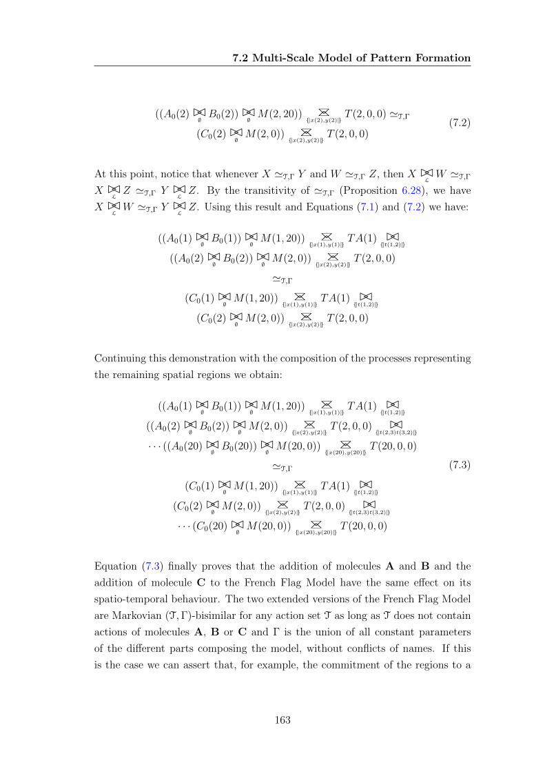
7.2 Multi-Scale Model of Pattern Formation
((A0(2)BC∅B0(2))BC
∅M(2, 20)) BC
{|x(2),y(2)|}T (2, 0, 0) 'T,Γ
(C0(2)BC∅M(2, 0)) BC
{|x(2),y(2)|}T (2, 0, 0)
(7.2)
At this point, notice that whenever X 'T,Γ Y and W 'T,Γ Z, then X BCLW 'T,Γ
X BCLZ 'T,Γ Y BC
LZ. By the transitivity of 'T,Γ (Proposition 6.28), we have
X BCLW 'T,Γ Y BC
LZ. Using this result and Equations (7.1) and (7.2) we have:
((A0(1)BC∅B0(1))BC
∅M(1, 20)) BC
{|x(1),y(1)|}TA(1) BC
{|t(1,2)|}
((A0(2)BC∅B0(2))BC
∅M(2, 0)) BC
{|x(2),y(2)|}T (2, 0, 0)
'T,Γ
(C0(1)BC∅M(1, 20)) BC
{|x(1),y(1)|}TA(1) BC
{|t(1,2)|}
(C0(2)BC∅M(2, 0)) BC
{|x(2),y(2)|}T (2, 0, 0)
Continuing this demonstration with the composition of the processes representing
the remaining spatial regions we obtain:
((A0(1)BC∅B0(1))BC
∅M(1, 20)) BC
{|x(1),y(1)|}TA(1) BC
{|t(1,2)|}
((A0(2)BC∅B0(2))BC
∅M(2, 0)) BC
{|x(2),y(2)|}T (2, 0, 0) BC
{|t(2,3)t(3,2)|}
· · · ((A0(20)BC∅B0(20))BC
∅M(20, 0)) BC
{|x(20),y(20)|}T (20, 0, 0)
'T,Γ
(C0(1)BC∅M(1, 20)) BC
{|x(1),y(1)|}TA(1) BC
{|t(1,2)|}
(C0(2)BC∅M(2, 0)) BC
{|x(2),y(2)|}T (2, 0, 0) BC
{|t(2,3)t(3,2)|}
· · · (C0(20)BC∅M(20, 0)) BC
{|x(20),y(20)|}T (20, 0, 0)
(7.3)
Equation (7.3) finally proves that the addition of molecules A and B and the
addition of molecule C to the French Flag Model have the same effect on its
spatio-temporal behaviour. The two extended versions of the French Flag Model
are Markovian (T,Γ)-bisimilar for any action set T as long as T does not contain
actions of molecules A, B or C and Γ is the union of all constant parameters
of the different parts composing the model, without conflicts of names. If this
is the case we can assert that, for example, the commitment of the regions to a
163
7.3 Multi-Scale Model of Tissue Growth
specialisation (T = {|mem(1), . . . ,mem(20)|}) happens with the same timing and
with the same probability in both models.
7.3 Multi-Scale Model of Tissue Growth
We now turn our attention to a multi-scale model of tissue growth. This model is
constructed in analogy with our earlier tissue growth model introduced in Section
4.2.3 and modelled in process algebra with hooks in Section 5.1.3. We define it
as a multi-scale model because two scales are present, tissue and biochemistry,
and the two scales need to interact. In particular, we show how one can define
a model where growth and death of tissue depend on the local concentration of
biochemical species. Here we give an overview of the model, while leaving the
complete specification in Appendix B.1.
At the tissue scale we consider an area divided into regions of the same size and
shape. We consider a grid of 10 × 10 regions, each region is denoted by R(i, j).
Each region can be empty (agent E(i, j)) or contain tissue. There are four types
of tissue: tissue that can neither grow nor die (agent T (i, j)); tissue that can
grow, but not die (Tm(i, j)); tissue that can die but not grow (Ta(i, j)); tissue
that can both grow and die (Tam(i, j)). Tissue processes change between these
four agents depending on the configuration of the biochemical scale. The event of
growth is represented by action growth(i, j, i2, j2) which is performed by a tissue
agent in region R(i, j) in synchronisation with an adjacent empty space E(i2, j2)
in region R(i2, j2). Two regions are considered adjacent if they share an edge.
If no adjacent region is empty, growth is inhibited. The event of tissue death is
represented by action death(i, j). We assume that actions growth(i, j, i2, j2) and
death(i, j) have constant rates kgrowth and kdeath .
The biochemical scale consists of biochemical species A, B and C, present
in all regions. The concentration of each species varies between a concentration
level of 0 and 10 (parameter maxLevels = 10). In particular, we use agent
A(i, j, w) to denote that species A in region R(i, j) presents concentration level
w. Analogously for species B and C. Concentration level of the three species
can change because of the following local biochemical reactions (and associated
velocities):
164
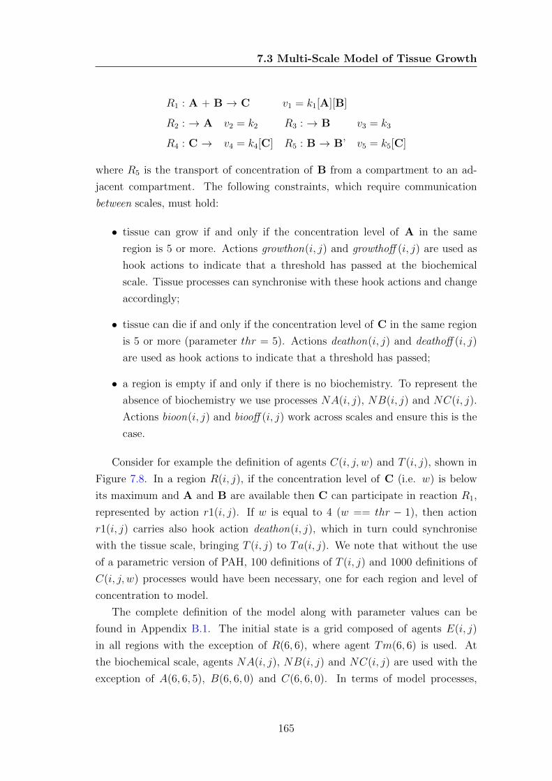
7.3 Multi-Scale Model of Tissue Growth
R1 : A + B → C v1 = k1[A][B]
R2 : → A v2 = k2 R3 : → B v3 = k3
R4 : C → v4 = k4[C] R5 : B → B’ v5 = k5[C]
where R5 is the transport of concentration of B from a compartment to an ad-
jacent compartment. The following constraints, which require communication
between scales, must hold:
• tissue can grow if and only if the concentration level of A in the same
region is 5 or more. Actions growthon(i, j) and growthoff (i, j) are used as
hook actions to indicate that a threshold has passed at the biochemical
scale. Tissue processes can synchronise with these hook actions and change
accordingly;
• tissue can die if and only if the concentration level of C in the same region
is 5 or more (parameter thr = 5). Actions deathon(i, j) and deathoff (i, j)
are used as hook actions to indicate that a threshold has passed;
• a region is empty if and only if there is no biochemistry. To represent the
absence of biochemistry we use processes NA(i, j), NB(i, j) and NC(i, j).
Actions bioon(i, j) and biooff (i, j) work across scales and ensure this is the
case.
Consider for example the definition of agents C(i, j, w) and T (i, j), shown in
Figure 7.8. In a region R(i, j), if the concentration level of C (i.e. w) is below
its maximum and A and B are available then C can participate in reaction R1,
represented by action r1(i, j). If w is equal to 4 (w == thr − 1), then action
r1(i, j) carries also hook action deathon(i, j), which in turn could synchronise
with the tissue scale, bringing T (i, j) to Ta(i, j). We note that without the use
of a parametric version of PAH, 100 definitions of T (i, j) and 1000 definitions of
C(i, j, w) processes would have been necessary, one for each region and level of
concentration to model.
The complete definition of the model along with parameter values can be
found in Appendix B.1. The initial state is a grid composed of agents E(i, j)
in all regions with the exception of R(6, 6), where agent Tm(6, 6) is used. At
the biochemical scale, agents NA(i, j), NB(i, j) and NC(i, j) are used with the
exception of A(6, 6, 5), B(6, 6, 0) and C(6, 6, 0). In terms of model processes,
165
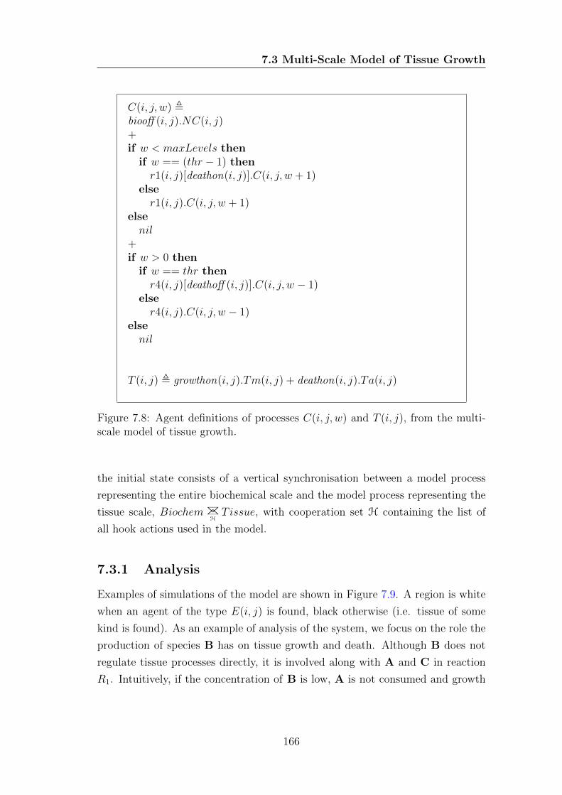
7.3 Multi-Scale Model of Tissue Growth
C(i, j, w) ,biooff (i, j).NC(i, j)+if w < maxLevels then
if w == (thr − 1) thenr1(i, j)[deathon(i, j)].C(i, j, w + 1)
elser1(i, j).C(i, j, w + 1)
elsenil
+if w > 0 then
if w == thr thenr4(i, j)[deathoff (i, j)].C(i, j, w − 1)
elser4(i, j).C(i, j, w − 1)
elsenil
T (i, j) , growthon(i, j).Tm(i, j) + deathon(i, j).Ta(i, j)
Figure 7.8: Agent definitions of processes C(i, j, w) and T (i, j), from the multi-scale model of tissue growth.
the initial state consists of a vertical synchronisation between a model process
representing the entire biochemical scale and the model process representing the
tissue scale, Biochem BC
HTissue, with cooperation set H containing the list of
all hook actions used in the model.
7.3.1 Analysis
Examples of simulations of the model are shown in Figure 7.9. A region is white
when an agent of the type E(i, j) is found, black otherwise (i.e. tissue of some
kind is found). As an example of analysis of the system, we focus on the role the
production of species B has on tissue growth and death. Although B does not
regulate tissue processes directly, it is involved along with A and C in reaction
R1. Intuitively, if the concentration of B is low, A is not consumed and growth
166
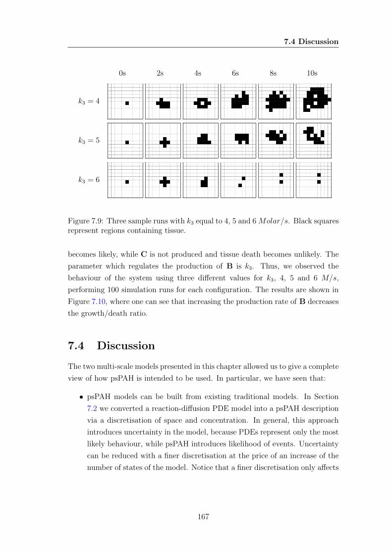
7.4 Discussion
0s 2s 4s 6s 8s 10s
k3 = 4
k3 = 5
k3 = 6
Figure 7.9: Three sample runs with k3 equal to 4, 5 and 6 Molar/s. Black squaresrepresent regions containing tissue.
becomes likely, while C is not produced and tissue death becomes unlikely. The
parameter which regulates the production of B is k3. Thus, we observed the
behaviour of the system using three different values for k3, 4, 5 and 6 M/s,
performing 100 simulation runs for each configuration. The results are shown in
Figure 7.10, where one can see that increasing the production rate of B decreases
the growth/death ratio.
7.4 Discussion
The two multi-scale models presented in this chapter allowed us to give a complete
view of how psPAH is intended to be used. In particular, we have seen that:
• psPAH models can be built from existing traditional models. In Section
7.2 we converted a reaction-diffusion PDE model into a psPAH description
via a discretisation of space and concentration. In general, this approach
introduces uncertainty in the model, because PDEs represent only the most
likely behaviour, while psPAH introduces likelihood of events. Uncertainty
can be reduced with a finer discretisation at the price of an increase of the
number of states of the model. Notice that a finer discretisation only affects
167
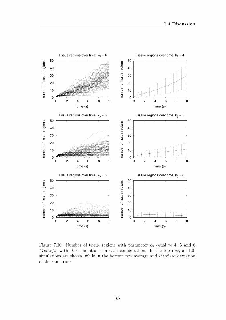
7.4 Discussion
0
10
20
30
40
50
0 2 4 6 8 10
nu
mbe
r o
f tissue r
egio
ns
time (s)
Tissue regions over time, k3 = 4
0
10
20
30
40
50
0 2 4 6 8 10
nu
mbe
r o
f tissue r
egio
ns
time (s)
Tissue regions over time, k3 = 4
0
10
20
30
40
50
0 2 4 6 8 10
num
ber
of tissue r
egio
ns
time (s)
Tissue regions over time, k3 = 5
0
10
20
30
40
50
0 2 4 6 8 10
num
ber
of tissue r
egio
ns
time (s)
Tissue regions over time, k3 = 5
0
10
20
30
40
50
0 2 4 6 8 10
nu
mbe
r of tissue r
egio
ns
time (s)
Tissue regions over time, k3 = 6
0
10
20
30
40
50
0 2 4 6 8 10
nu
mbe
r of tissue r
egio
ns
time (s)
Tissue regions over time, k3 = 6
Figure 7.10: Number of tissue regions with parameter k3 equal to 4, 5 and 6Molar/s, with 100 simulations for each configuration. In the top row, all 100simulations are shown, while in the bottom row average and standard deviationof the same runs.
168
7.4 Discussion
the size of the initial state of the psPAH model, while the parametric agent
definitions are unaltered;
• additional scales can be easily added to existing models using process al-
gebra compositionality. In Section 7.2, we converted the biochemical scale
model of diffusion and degradation of morphogen M into a psPAH descrip-
tion and subsequently augmented it with explicit representations of tissue
and commitment to tissue specialisations;
• psPAH forces an explicit representation of scales and actions between and
within scales, resulting in an explicit multi-scale compositionality. In both
models of pattern formation and tissue growth, processes on different scales
are clearly distinguishable because of the use of the BC
Loperator. While in
the first model we distributed BC
Lover the spatial regions, in the second
model we used BC
Lonly once, defining a clear distinction between the bio-
chemical and tissue scales. This latter approach guarantees a multi-scale
compositionality of the model, where a scale can be easily substituted with
another. Notice that this approach is also possible in the first model, though
an additional layer is required to manage multiple hook actions (t(i, j) may
offer both y(i) and x(j) at the same time);
• a psPAH model can be analysed with traditional techniques. We analysed
the behaviour of both models quantitatively using stochastic simulations.
An example of sensitivity analysis was also given in the tissue growth exam-
ple, where a constant parameter was altered at the biochemical scale and
change in quantitative behaviour was observed at the tissue scale;
• qualitative information about quantitative behaviour can be derived us-
ing process algebra related techniques. In Section 7.2.2 we proved that
two extensions of the French Flag Model have the same spatio-temporal
behaviour, without investigating their behaviour quantitatively. Moreover,
this was achieved by simply observing that just a small part of the two mod-
els was equivalent and then proving that this equivalence could be extended
to the entire models.
169
7.5 Summary
7.5 Summary
In this section we have illustrated the use of process algebra with hooks to define
and simulate multi scale models of pattern formation and tissue growth. In order
to define the models compactly we extended the algebra with parametric processes
and actions and with the if-then-else construct. We illustrated how parametric
stochastic process algebra with hooks can be used to model and analyse two multi-
scale scenarios: pattern formation and tissue growth. Finally, we highlighted the
benefits of using a process algebraic approach in these scenarios. Most notably,
we have seen how one can manipulate models and reason on their behaviour using
process algebra with hooks compositionality and theoretical results.
170
Chapter 8
Conclusions
The multi-scale modelling of biological systems consists of the integration in the
same model of multiple levels of detail, from molecules, to cells, to tissues and so
on. Usually, different levels of detail are represented by different mathematical
approaches, e.g. concentration of molecules by ordinary differential equations,
evolution of tissue by cellular automata. Moreover, models are often tailored
around the specific system under study. As a result, multi-scale models are
difficult to write, maintain, share, compose and compare.
In this thesis we have demonstrated that process algebra, and in particular
process algebra with hooks, provides an effective mathematical framework to
construct, compose and compare multi-scale models.
First, we investigated the use of a simple process algebra to model a single scale
of a biological phenomenon, focussing on biochemical reactions and tissue growth.
As a result of this investigation, we proposed a novel approach to functional rates
in process algebra with multi-way synchronisation, where we assume that actions
can be rated only when all the expected participants synchronise. In addition,
we considered the use of parameters to reduce the length of definitions in models
with repetitive process definition, which is often the case if concentration levels
and geometrical space are considered.
Second, we investigated the use of the simple process algebra and a process
algebra with priorities to model multi-scale scenarios, with attention to the in-
teractions between scales and the representation of thresholds. In particular, we
assumed that the quantitative behaviour at a scale affects other scales only when
certain configurations or states are reached, for example when one or more bio-
171
chemical species passes a concentration threshold. We observed that the simple
process algebra encountered a combinatorial problem in the process definition
when multiple thresholds are considered. Conversely, the process algebra with
priority showed to possess mechanisms able to represent effectively both inter-
actions within and between scales. However, we demonstrated that the style
of modelling of process algebra with priorities presented drawbacks which, in a
multi-scale scenario, require to be addressed. The drawbacks are: the introduc-
tion of intermediate and biologically meaningless states; the lack of control by
the modeller on the response to simultaneous inter-scale events; the lack of syn-
tactic elements that can define unambiguously scales and interactions within and
between scales.
Third, we proposed process algebra with hooks for multi-scale modelling of
biological systems. Building up from our investigations, we defined this algebra
to address the drawbacks of process algebra with priorities and to support our
approach to functional rates. Characteristics of the algebra are the use of com-
posed actions and a novel vertical composition operator. In addition, we defined
three congruence relations on process algebra with hooks. In particular, one of
them, Markovian (T,Γ)-bisimulation, has been designed to relate models that
present the same behaviour at a specified scale, at the same time with the same
probability. Most notably, our approach to functional rates was fundamental to
the proof of congruence.
Finally, we illustrated the use of process algebra with hooks to define, compose
and relate models of pattern formation and tissue growth.
With the above results we demonstrated that:
• define. Process algebra with hooks can be used independently of the scale
one decides to model first. Each scale can be treated as the same formal
object: a process. For example, we modelled the biochemical scale (Section
5.2.3) or the tissue scale (Section 5.2.4);
• compose. Composition of scales is facilitated by the intrinsic composition-
ality of the process algebra approach and by the novel vertical cooperation
operator. Interactions between scales are unambiguously identified by hook
actions. For example, we modelled interactions between the biochemical
scale and the tissue scale in Sections 7.2 and 7.3;
172
8.1 Future Directions
• relate. The framework of process algebra with hooks allows formal reason-
ing about behaviour of models. As a consequence, relations can be defined
between models, capturing a specified degree of equality or similarity. In
particular, we defined three equivalence relations in Sections 6.2.1 and 6.2.2
and we illustrated how one of them can be used to infer qualitative infor-
mation about quantitative behaviour in Section 7.2.2.
Although we have set the foundations of process algebra with hooks for multi-
scale models, further research is necessary before it can be considered as com-
petitive as other more consolidated mathematical approaches. At present, three
challenges need to be addressed. First, an efficient stochastic simulation algo-
rithm needs to be defined, in order to allow modelling of large systems and un-
derstand the time and space complexity limitations of using process algebra with
hooks. Second, other equivalence relations should be defined. The ability to
relate models and their behaviour is the most appealing feature of the process
algebra approach. Although we defined three fundamental relations, these may
be too strong to relate biological systems, where often one is interested in how
similar two models are, rather than whether they are exactly the same. The time
complexity of testing of the equalities has also to be investigated. Finally, pro-
cess algebra with hooks needs to be compared with state of the art approaches
to multi-scale modelling. This will be possible only once the two previous points
are addressed. Without efficient simulations and flexible equivalence relations it
would be difficult to quantify differences in time complexity and model manipu-
lation.
In the following section we outline how one should proceed to address the
above lines of research.
8.1 Future Directions
• efficient stochastic simulations of process algebra with hooks models. At
the moment, the simulator that samples trajectories of transitions is not
optimised. In fact, at each step the complete set of rated transitions is
computed, while it could be the case that only a few processes are affected
by the last step and that only a few transitions need to be updated. A first
improvement is to determine which processes are affected by a transition.
173
8.2 Summary
With this information, improvements to stochastic simulations of biochemi-
cal reactions and their diffusion, e.g. (Elf and Ehrenberg, 2004; Gibson and
Bruck, 2000), can be adapted and integrated in our approach;
• definition of approximate relations on process algebra with hooks processes.
We may require a more qualitative interpretation of behaviour, where two
systems can be considered similar, though not identical. Approximate
equivalence relations (Tini, 2010) and distance measures between models
may prove an interesting direction to explore if we want to compare bio-
logical systems. Parameters that identify positions could be used to define
metrics for approximate equivalence relations;
• Comparison of process algebra with hooks with other approaches. The above
two points will have to be developed in order to have a fair comparison.
Consider, for example, the case of comparing process algebra with hooks
with cellular automata. Fundamental to cellular automata is the ability
to provide fast simulations of large systems, while it does not provide the
mathematical framework of process algebra. In order to compare the two
approaches, one needs to determine how the time complexity of optimised
simulations of process algebra with hooks models compares with that of cel-
lular automata, and what flexible relations on processes provide a practical
advantage.
8.2 Summary
We have developed and illustrated the use of a novel process algebra designed
for multi-scale modelling of biological systems. Its mathematical framework pro-
vides a flexible environment where quantitative, dynamic, multi-scale models of
biological systems can be defined, composed and compared.
We have provided the foundations of a new approach; future work is required
to determine its full potential.
174
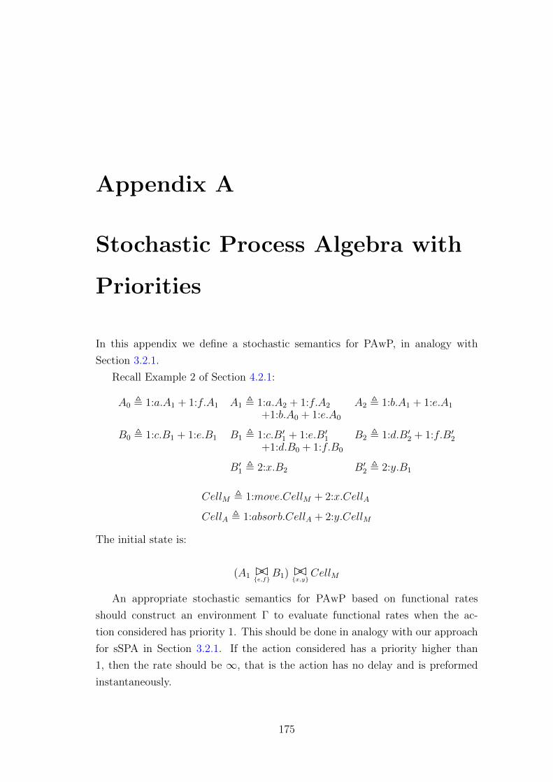
Appendix A
Stochastic Process Algebra with
Priorities
In this appendix we define a stochastic semantics for PAwP, in analogy with
Section 3.2.1.
Recall Example 2 of Section 4.2.1:
A0 , 1:a.A1 + 1:f.A1 A1 , 1:a.A2 + 1:f.A2 A2 , 1:b.A1 + 1:e.A1
+1:b.A0 + 1:e.A0
B0 , 1:c.B1 + 1:e.B1 B1 , 1:c.B′1 + 1:e.B′1 B2 , 1:d.B′2 + 1:f.B′2+1:d.B0 + 1:f.B0
B′1 , 2:x.B2 B′2 , 2:y.B1
CellM , 1:move.CellM + 2:x.CellA
CellA , 1:absorb.CellA + 2:y.CellM
The initial state is:
(A1 BC{e,f}B1) BC{x,y}
CellM
An appropriate stochastic semantics for PAwP based on functional rates
should construct an environment Γ to evaluate functional rates when the ac-
tion considered has priority 1. This should be done in analogy with our approach
for sSPA in Section 3.2.1. If the action considered has a priority higher than
1, then the rate should be ∞, that is the action has no delay and is preformed
instantaneously.
175
As in Section 3.2.1 we assign variables and values to agents:
Var(A0) = A Var(B0) = B Var(B′1) = B Var(CellM) = cell
Val(A0) = 0 Val(B0) = 0 Val(B′1) = 2 Val(CellM) = 1
Var(A1) = A Var(B1) = B Var(B′2) = B Var(CellA) = cell
Val(A1) = 1 Val(B1) = 1 Val(B′2) = 1 Val(CellA) = 2
Var(A2) = A Var(B2) = B
Val(A2) = 2 Val(B2) = 2
Functional rates and sets of participants for actions are:
fa = ka/h pa = {A} ff = (kf ∗B ∗ h)/h pf = {A,B}
fb = (kb ∗ A ∗ h)/h pb = {A} fmove = kmove pmove = {cell}
fc = kc/h pc = {B} fabsorb = kabsorb pabsorb = {cell}
fd = (kd ∗B ∗ h)/h pd = {B} fx =∞ px = {B, cell}
fe = (ke ∗ A ∗ h)/h pe = {A,B} fy =∞ py = {B, cell}
A valid derivation for the above example should be:
(A1 BC{e,f}B1) BC{x,y}
CellM(1:b,Γ)−−−→ (A0 BC{e,f}B1) BC
{x,y}CellM
where Γ = {(A, 1)}. From state (A1 BC{e,f}B′1) BC{x,y}
CellM the only derivation pos-
sible should be:
(A1 BC{e,f}B′1) BC{x,y}
CellM(2:x,Γ′)−−−−→ (A1 BC{e,f}B2) BC
{x,y}CellA
where Γ′ = {(B, 2), (cell, 1)}. Although Γ′ is not used to evaluate fx, it is neces-
sary to verify that envV ar(Γ′)= px, i.e. that the variable contained in Γ are ex-
actly the variables contained in the set of participants px. The operation of rating
should then distinguish between actions with priority 1 and actions with priority
higher than 1. This means that valid transitions should carry the priority of the
action on their label. Using the additional environment Γ = {(h, 1), (ka, 1), (kb, 1),
(kc, 1), (kd, 1), (ke, 1), (kf , 1), (kmove, 1), (kabsorb, 1)}, two examples of rated transi-
tions should be:
176
(A1 BC{e,f}B1) BC{x,y}
CellM(b,1)−−→ (A0 BC{e,f}B1) BC
{x,y}CellM
(A1 BC{e,f}B′1) BC{x,y}
CellM(x,∞)−−−→ (A1 BC{e,f}B2) BC
{x,y}CellA
where the priority of the actions is now not necessary and so dropped.
Recall that we are assuming that we can always determine all the biological
entities that interact for a specific event. This allows us to identify unequivocally
which processes will participate to an action in a certain moment. This is our
assumption for biological interactions within a scale. However, this might not hold
in the case of interactions between scales via instantaneous actions. Consider the
following example:
A , 1:a.A′ B , 1:b.B′ C , 2:x.C ′
A′ , 2:x.A′′ B′ , 2:x.B′′
Var(A) = levelA Var(B) = levelB Var(C) = celltype
Var(A′) = levelA Var(B′) = levelB
with initial state:
(ABC∅B)BC
{x}C
Assume now that processes A and B represent the biochemical scale and C the
cellular scale. In this example, the condition for C to change its state is that either
A performs action a or B performs action b. This implies that the instantaneous
action x can have two different sets of participants, that is {levelA, celltype} and
{levelB, celltype}. In order to allow the determination of the correct participants
to instantaneous actions, we impose that if fx = ∞ then the set of participants
px is a set of sets of parameter names. In this case we have:
fa = ka/h pa = {levelA}
fb = kb/h pb = {levelB}
fx =∞ px = {{levelA, celltype}, {levelB, celltype}}
Another constraint we have to impose is that given prioritised action p:x,
fx = ∞ if and only if p > 1. This way, instantaneous actions are exactly all
actions with priority higher than 1.
177
A.1 Stochastic Process Algebra with Priorities
A.1 Stochastic Process Algebra with Priorities
In analogy with Section 3.2.1 we proceed to the definition of a new syntax and
semantics for PAwP. The syntax is given by:
D ::= nil | p:a.A | D +D
M ::= A |M BCLM
where:
• D is a definition process, D ∈ Pd, while M is a model process, M ∈ Pm.
Definition and model processes are disjoint and are both processes, i.e.
Pd ∪ Pm = P and Pd ∩ Pm = ∅;
• Agents are defined as A , D, that is we use definition processes to define
the behaviour of agents;
• a model is defined by a model process M , which in turn is either an agent
A or a cooperation between model processes M BCLM ;
• action execution p:a.A is always followed by an agent A. This ensures that
at any time the state of a model will be constituted of cooperations of
agents;
• functions Var(A) and Val(A) must be defined for each agent A, with
Var(A) ∈ Names, Val(A) ∈ R and Names the set of parameter names.
In order to define a stochastic semantics for this new syntax, we use the
following additional definitions:
• PM(M), M ∈ Pm, returns the potential moves of a process M , PM(M) ⊆(N \ {0}) × Actions × 2Names×R × Pm. PM(M) is defined by structural
induction as:
178
A.1 Stochastic Process Algebra with Priorities
PM(nil) = ∅
PM(p:a.A) = {|(p, a, A)|}
PM(D1 +D2) = PM(D1) ] PM(D2)
PM(A) = {|(p, a,Γ, A) | (p, a, A) ∈ PM(D) ∧ A , D ∧ Γ = {(Var(A),Val(A))}|}
PM(M1 BCLM2) = {|(p, a,Γ,M ′
1BCLM2) | (p, a,Γ,M ′
1) ∈ PM(M1) ∧ a 6∈ L|}
]{|(p, a,Γ,M1 BCLM ′
2) | (p, a,Γ,M ′2) ∈ PM(M2) ∧ a 6∈ L|}
]{|(p, a,Γ1 ∪ Γ2,M′1BCLM ′
2) | (p, a,Γ1,M′1) ∈ PM(M1)
∧(p, a,Γ2,M′2) ∈ PM(M2) ∧ a ∈ L|}
• Select(PM(M)) returns the potential moves of M with the highest priority
and is defined as:
Select(PMSet) = {|(p, a,Γ,M) | (p, a,Γ,M) ∈ PMSet ∧ ∀(q, b,Γ′,M ′) ∈PMSet.p ≥ q|}
Using the functions defined above, a stochastic semantics for PAwP of actions
and functional rates is given by the following derivation rule:
(p, a,Γ,M ′) ∈ Select(PM(M))
M(p:a,Γ)−−−−→M ′
We refer to this new process algebra as stochastic process algebra with prior-
ities (sPAwP). Most of the definitions we introduced in Section 3.2.1 are almost
unchanged. The definitions differ only in the fact that they need to consider
priorities and instantaneous actions, with rate ∞.
Definition A.1 Activity. The couple (p:a,Γ) such that p ∈ (N \ {0}), a ∈Actions and Γ ⊆ Names× R is called an activity.
Definition A.2 One step derivative. If M(p:a,Γ)−−−−→ M ′ then M is a one step
derivative of M .
Definition A.3 Derivative. If Mi(p:a,Γ)−−−−→ . . .
(p′:a′,Γ′)−−−−−→Mj then Mj is a derivative
of Mi.
179
A.1 Stochastic Process Algebra with Priorities
Definition A.4 Derivative Set. The derivative set of a model process M ∈ Pmis denoted by ds(M) and is defined as the smallest set of model processes such
that:
• M ∈ ds(M);
• if Mi ∈ ds(M) and Mi(p:a,Γ)−−−−→Mj then Mj ∈ ds(M).
Definition A.5 Current activities for model Processes. The set of activities
that M ∈ Pm can perform is denoted by Activities(M) and is defined as:
Activities(M) = {|(p:a,Γ) | (p, a,Γ,M ′) ∈ Select(PM(M))|}
Definition A.6 Activity set. The set of all activities that a model process
M ∈ Pm or one of its derivatives can perform is given by:
−−−−−−→Activities(M) =
⊎Mi∈ds(M)
Activities(Mi)
Definition A.7 Derivation graph. Given a model component M ∈ Pm, the
derivation graph D(M) is the labelled directed graph with:
• set of nodes ds(M);
• multi set of transition labels−−−−−−→Activities(M);
• multi set of labelled transitions→⊆ ds(M)×−−−−−−→Activities(M)×ds(M). Given
M ′ ∈ ds(M), (M ′, p:a,Γ,M ′′) ∈→ iff M ′ (p:a,Γ)−−−−→M ′′.
Definition A.8 Open activity. An open activity is an activity (p:a,Γ) where:
• if p = 1 then Γ does not contain the exact variables present in the partici-
pant set pa, i.e. envVar(Γ)6= pa;
• if p 6= 1 then the set of variables contained in Γ is not in the set of possible
sets of participants pa, i.e. envVar(Γ)6∈ pa.
180
A.1 Stochastic Process Algebra with Priorities
Definition A.9 Function openActivities. The function ‘openActivities’ selects
open activities from a set of activities A ⊆ (N \ {0})× Actions× 2Names×R:
openActivities(A)= {|(p:a,Γ) | ((p = 1 ∧ envVar(Γ) 6= pa)
∨(p 6= 1 ∧ envVar(Γ) 6∈ pa)) ∧ (p:a,Γ) ∈ A|}
Definition A.10 Current open activities. Given a model process M ∈ Pm, the
set of open activities that P can perform is defined as:
OpenAct(M) = openActivities(Activities(M))
Definition A.11 Open activity set. The set of all open activities that a model
process M ∈ Pm can perform is given by:
−−−−−−→OpenAct(M) = openActivities(
−−−−−−→Activities(M))
Definition A.12 Closed activity. A closed activity is an activity (p:a,Γ) where
:
• if p = 1 then Γ contains the exact variables present in the participant set
pa, i.e. envVar(Γ)= pa;
• if p 6= 1 then the set of variables contained in Γ is in the set of possible sets
of participants pa, i.e. envVar(Γ)∈ pa.
Definition A.13 Function closedActivities. The function ‘closedActivities’ se-
lects closed activities from a set of activities A ⊆ (N\{0})×Actions×2Names×R:
closedActivities(A) = (A \ openActivities(A))
Definition A.14 Current closed activities. Given a model process M ∈ Pm, the
set of closed activities that M can perform is defined as:
ClosedAct(M) = closedActivities(Activities(M))
181
A.1 Stochastic Process Algebra with Priorities
Definition A.15 Closed activity set. The set of all open activities that a model
process M ∈ Pm can perform is given by:
−−−−−−−→ClosedAct(M) = closedActivities(
−−−−−−→Activities(M))
Definition A.16 Rated activity. The couple (a, r) such that a ∈ Actions and
r ∈ R>0 ∪ {∞} is called a rated activity.
Definition A.17 Function rateActivities. Given an environment Γ, “rateAc-
tivities” converts a set of activities A ⊆ (N \ {0}) × Actions × 2Names×R into a
set of rated activities B ⊆ Actions× (R ∪ {∞}):
rateActivities(Γ)(A) =
{|(a, ra) | ((Γ ∪ Γ′ ` fa → k ∧ ra = k/π(A, (p:a,Γ′)) ∧ p = 1)
∨(p 6= 1 ∧ ra =∞)) ∧ (p:a,Γ′) ∈ A ∧ fa ∈ F|}
where π(A, (p:a,Γ′)) returns the number of occurrences of (p:a,Γ′) in the multi
set A.
Definition A.18 Current rated activities. Given a model process M ∈ Pm and
an environment Γ ⊆ 2Names×R, the set of rated activities that M can perform is
defined as:
RatedAct(M)Γ = rateActivities(Γ)(ClosedAct(M))
RatedAct(M)Γ can be written RatedAct(M) if Γ is clear from the context.
Definition A.19 Rated activity set. Given an environment Γ ⊆ 2Names×R, the
set of all rated activities that a model process M ∈ Pm can perform is given by:
−−−−−−→RatedAct(M)Γ = rateActivity(Γ)(
−−−−−−−→ClosedAct(M))
−−−−−−→RatedAct(M)Γ can be written
−−−−−−→RatedAct(M) if Γ is clear from the context.
Definition A.20 Rated derivation graph. Given a model process M ∈ Pm and
an environment Γ ⊆ 2Names×R, the rated derivation graph Dr(M)Γ is the labelled
directed graph with:
182
A.1 Stochastic Process Algebra with Priorities
• set of nodes ds(M);
• multi set of transition labels−−−−−−→RatedAct(M)Γ;
• multi set of labelled transitions →r⊆ ds(M) ×−−−−−−→RatedAct(M)Γ × ds(M).
Given M ′ ∈ ds(M), (M ′, a, ra,M′′) ∈→r iff M ′ (p:a,Γ′)−−−−→ M ′′, (p:a,Γ′) ∈
ClosedAct(M) and {|(a, k)|} = rateActivities(Γ)({|(p:a,Γ′)|}) and
ra = k/π(ClosedAct(M), (p:a,Γ′)).
• multi set of labelled transitions→o⊆ ds(M)×−−−−−−→OpenAct(M)×ds(M). Given
M ′ ∈ ds(M), (M ′, p:a,Γ′,M ′′) ∈→o iff M ′ (p:a,Γ′)−−−−→ M ′′ and (p:a,Γ′) ∈OpenAct(M).
Dr(M)Γ can be written Dr(M) if Γ is clear from the context.
183
Appendix B
Case Study Complete Model
Definitions
B.1 Detailed Definition of the Multi-Scale Model
of Tissue Growth
In this section we provide the complete definition of the multi-scale model of
tissue growth presented in Section 7.3
Constants:
k1 = 1/(Ms) k2 = 5 M/s k3 = 5 M/s
k4 = 1/s k5 = 1/s h = 1 M
kdeath = 1 event/s kgrowth = 1 event/s maxLevels = 10
rows = 10 cols = 10 thr = 5
Functional rates and sets of participants:
fr1(i,j) = k1 ∗ A(i, j) ∗ h ∗B(i, j) ∗ h/h
pr1(i,j) = {A(i, j), B(i, j), C(i, j)}
fr2(i,j) = k2/h
pr2(i,j) = {A(i, j)}
fr3(i,j) = k3/h
184
B.1 Detailed Definition of the Multi-Scale Model of Tissue Growth
pr3(i,j) = {B(i, j)}
fr4(i,j) = k4 ∗ C(i, j) ∗ h/h
pr4(i,j) = {C(i, j)}
fr5(i,j,i2,j2) = k5 ∗B(i, j) ∗ h/h
pr5(i,j) = {B(i, j), B(i2, j2)}
fdeath(i,j) = kdeath
pdeath(i,j) = {R(i, j)}
fgrowth(i,j,i2,j2) = kgrowth
pgrowth(i,j,i2,j2) = {R(i, j), R(i2, j2)}
Agent definitions:
NA(i, j) , bioon(i, j).A(i, j, 0)
A(i, j, w) , biooff (i, j).NA(i, j)
+(
if w < maxLevels then
if w == (thr − 1) then
r2(i, j)[growthon(i, j)].A(i, j, w + 1)
else r2(i, j).A(i, j, w + 1)
else nil)
+(
if w > 0 then
if w == thr then
r1(i, j)[growthoff (i, j)].A(i, j, w − 1)
else r1(i, j).A(i, j, w − 1)
else nil)
NB(i, j) , bioon(i, j).B(i, j, 0)
185
B.1 Detailed Definition of the Multi-Scale Model of Tissue Growth
B(i, j, w) , biooff (i, j).NB(i, j)
+(
if w < maxLevels then
r3(i, j).B(i, j, w + 1)
+(if i > 1 then r5(i− 1, j, i, j).B(i, j, w + 1) else nil)
+(if i < rows then r5(i+ 1, j, i, j).B(i, j, w + 1) else nil)
+(if j > 1 then r5(i, j − 1, i, j).B(i, j, w + 1) else nil)
+(if j < cols then r5(i, j + 1, i, j).B(i, j, w + 1) else nil)
else nil)
+(
if w > 0 then
r1(i, j).B(i, j, w − 1)
+(if i > 1 then r5(i, j, i− 1, j).B(i, j, w − 1) else nil)
+(if i < rows then r5(i, j, i+ 1, j).B(i, j, w − 1) else nil)
+(if j > 1 then r5(i, j, i, j − 1).B(i, j, w − 1) else nil)
+(if j < cols then r5(i, j, i, j + 1).B(i, j, w − 1) else nil)
else nil)
NC(i, j) , bioon(i, j).C(i, j, 0)
C(i, j, w) , biooff (i, j).NC(i, j)
+(
if w < maxLevels then
if w == (thr − 1) then
r1(i, j)[deathon(i, j)].C(i, j, w + 1)
else r1(i, j).C(i, j, w + 1)
else nil)
+(
if w > 0 then
if w == thr then
186
B.1 Detailed Definition of the Multi-Scale Model of Tissue Growth
r4(i, j)[deathoff (i, j)].C(i, j, w − 1)
else r4(i, j).C(i, j, w − 1)
else nil)
E(i, j) ,
(if i > 1 then growth(i− 1, j, i, j)[bioon(i, j)].T (i, j) else nil)
+(if i < rows then growth(i+ 1, j, i, j)[bioon(i, j)].T (i, j) else nil)
+(if j > 1 then growth(i, j − 1, i, j)[bioon(i, j)].T (i, j) else nil)
+(if j < cols then growth(i, j + 1, i, j)[bioon(i, j)].T (i, j) else nil)
T (i, j) , growthon(i, j).Tm(i, j) + deathon(i, j).Ta(i, j)
Tm(i, j) ,
(if i > 1 then growth(i, j, i− 1, j).Tm(i, j) else nil)
+(if i < rows then growth(i, j, i+ 1, j).Tm(i, j) else nil)
+(if j > 1 then growth(i, j, i, j − 1).Tm(i, j) else nil)
+(if j < cols then growth(i, j, i, j + 1).Tm(i, j) else nil)
+growthoff (i, j).T (i, j) + deathon(i, j).Tam(i, j)
+{growthoff (i, j), deathon(i, j)}.Ta(i, j)
Ta(i, j) , death(i, j)[biooff (i, j)].E(i, j)
+apooff(i, j).T (i, j) +mitoon(i, j).Tam(i, j)
+{growthon(i, j), deathoff (i, j)}.Ta(i, j)
Tam(i, j), [R(i, j), 2] , death(i, j)[biooff (i, j)].E(i, j)
+(if i > 1 then growth(i, j, i− 1, j).Tam(i, j) else nil)
+(if i < rows then growth(i, j, i+ 1, j).Tam(i, j) else nil)
+(if j > 1 then growth(i, j, i, j − 1).Tam(i, j) else nil)
+(if j < cols then growth(i, j, i, j + 1).Tam(i, j) else nil)
+growthoff (i, j).Ta(i, j) + deathoff (i, j).Tm(i, j)
187
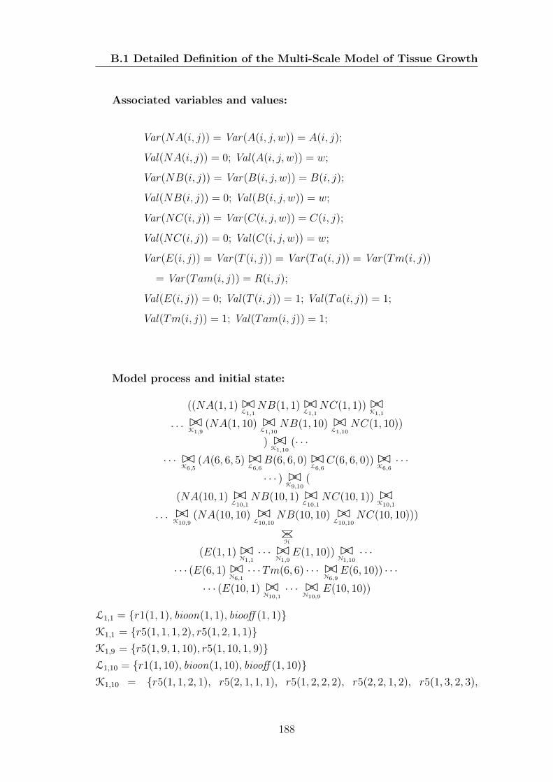
B.1 Detailed Definition of the Multi-Scale Model of Tissue Growth
Associated variables and values:
Var(NA(i, j)) = Var(A(i, j, w)) = A(i, j);
Val(NA(i, j)) = 0; Val(A(i, j, w)) = w;
Var(NB(i, j)) = Var(B(i, j, w)) = B(i, j);
Val(NB(i, j)) = 0; Val(B(i, j, w)) = w;
Var(NC(i, j)) = Var(C(i, j, w)) = C(i, j);
Val(NC(i, j)) = 0; Val(C(i, j, w)) = w;
Var(E(i, j)) = Var(T (i, j)) = Var(Ta(i, j)) = Var(Tm(i, j))
= Var(Tam(i, j)) = R(i, j);
Val(E(i, j)) = 0; Val(T (i, j)) = 1; Val(Ta(i, j)) = 1;
Val(Tm(i, j)) = 1; Val(Tam(i, j)) = 1;
Model process and initial state:
((NA(1, 1) BCL1,1
NB(1, 1) BCL1,1
NC(1, 1)) BCK1,1
. . . BCK1,9
(NA(1, 10) BCL1,10
NB(1, 10) BCL1,10
NC(1, 10))
) BCK1,10
(· · ·· · · BC
K6,5(A(6, 6, 5) BC
L6,6B(6, 6, 0) BC
L6,6C(6, 6, 0)) BC
K6,6· · ·
· · · ) BCK9,10
(
(NA(10, 1) BCL10,1
NB(10, 1) BCL10,1
NC(10, 1)) BCK10,1
. . . BCK10,9
(NA(10, 10) BCL10,10
NB(10, 10) BCL10,10
NC(10, 10)))
BC
H
(E(1, 1) BCN1,1· · · BC
N1,9E(1, 10)) BC
N1,10· · ·
· · · (E(6, 1) BCN6,1· · ·Tm(6, 6) · · · BC
N6,9E(6, 10)) · · ·
· · · (E(10, 1) BCN10,1· · · BC
N10,9E(10, 10))
L1,1 = {r1(1, 1), bioon(1, 1), biooff (1, 1)}K1,1 = {r5(1, 1, 1, 2), r5(1, 2, 1, 1)}K1,9 = {r5(1, 9, 1, 10), r5(1, 10, 1, 9)}L1,10 = {r1(1, 10), bioon(1, 10), biooff (1, 10)}K1,10 = {r5(1, 1, 2, 1), r5(2, 1, 1, 1), r5(1, 2, 2, 2), r5(2, 2, 1, 2), r5(1, 3, 2, 3),
188
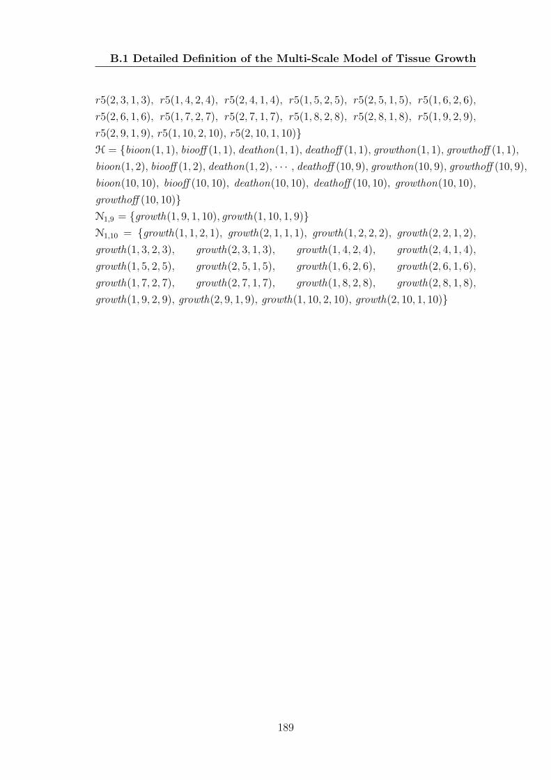
B.1 Detailed Definition of the Multi-Scale Model of Tissue Growth
r5(2, 3, 1, 3), r5(1, 4, 2, 4), r5(2, 4, 1, 4), r5(1, 5, 2, 5), r5(2, 5, 1, 5), r5(1, 6, 2, 6),
r5(2, 6, 1, 6), r5(1, 7, 2, 7), r5(2, 7, 1, 7), r5(1, 8, 2, 8), r5(2, 8, 1, 8), r5(1, 9, 2, 9),
r5(2, 9, 1, 9), r5(1, 10, 2, 10), r5(2, 10, 1, 10)}H = {bioon(1, 1), biooff (1, 1), deathon(1, 1), deathoff (1, 1), growthon(1, 1), growthoff (1, 1),
bioon(1, 2), biooff (1, 2), deathon(1, 2), · · · , deathoff (10, 9), growthon(10, 9), growthoff (10, 9),
bioon(10, 10), biooff (10, 10), deathon(10, 10), deathoff (10, 10), growthon(10, 10),
growthoff (10, 10)}N1,9 = {growth(1, 9, 1, 10), growth(1, 10, 1, 9)}N1,10 = {growth(1, 1, 2, 1), growth(2, 1, 1, 1), growth(1, 2, 2, 2), growth(2, 2, 1, 2),
growth(1, 3, 2, 3), growth(2, 3, 1, 3), growth(1, 4, 2, 4), growth(2, 4, 1, 4),
growth(1, 5, 2, 5), growth(2, 5, 1, 5), growth(1, 6, 2, 6), growth(2, 6, 1, 6),
growth(1, 7, 2, 7), growth(2, 7, 1, 7), growth(1, 8, 2, 8), growth(2, 8, 1, 8),
growth(1, 9, 2, 9), growth(2, 9, 1, 9), growth(1, 10, 2, 10), growth(2, 10, 1, 10)}
189
References
U. Alon. An Introduction to Systems Biology. Chapman & Hall/CRC, July 2006.
154
C. Athale, Y. Mansury, and T. S. Deisboeck. Simulating the impact of a molecu-
lar ‘decision-process’ on cellular phenotype and multicellular patterns in brain
tumors. Journal of Theoretical Biology, 233:469–481, 2005. 26
J. C. M. Baeten, J. A. Bergstra, and J. W. Klop. Syntax and defining equations
for an interrupt mechanism in process algebra. Fundamenta Informaticae, IX:
127–168, 1986. 31
N. Barkai and S. Leibler. Biological rhythms: Circadian clocks limited by noise.
Nature, 403:267–268, 2000. 19
H. C. Berg. Random Walks in Biology. Princeton University Press, 1993. 24
M. Bernardo. Extended Markovian Process Algebra. In Lecture Notes in Com-
puter Science, volume 1119, pages 315–330, 1996. 58, 81, 140
M. L. Blinov, J. R. Faeder, B. Goldstein, and W. S. Hlavacek. BioNetGen: soft-
ware for rule-based modeling of signal transduction based on the interactions
of molecular domains. Bioinformatics, 20(17):3289–3291, 2004. 2, 35
L. Bortolussi. Stochastic concurrent constraint programming. In Electronic Notes
in Theoretical Computer Science, volume 164, pages 65–80, 2006. 2
G. E Briggs and J. B. S. Haldane. A note on the kinetics of enzyme action.
Biochem. J., 19:338–339, 1925. 14
M. Calder and J. Hillston. Process algebra modelling styles for biomolecular
processes. In Lecture Notes in Computer Science, volume 5750, pages 1–25,
2009. 4, 34
190
REFERENCES
M. Calder, S. Gilmore, and J. Hillston. Modelling the influence of RKIP on the
ERK signalling pathway using the stochastic process algebra PEPA. In Lecture
Notes in Computer Science, volume 4230, pages 1–23, 2006a. 3
M. Calder, V. Vyshemirsky, D. Gilbert, and R. Orton. Analysis of signalling
pathways using continuous time Markov chains. Transactions on Computa-
tional Systems Biology VI, 4220:44–67, 2006b. 21, 40
L. Calzone, F. Fages, and S. Soliman. Biocham: An environment for modelling
biological systems and formalizing experimental knowledge. Bioinformatics,
22:1805–1807, 2006. 2, 35
L. Cardelli. Brane calculi. In Lecture Notes in Bioinformatics, volume 3082,
pages 257–278, 2005. 3, 34
L. Cardelli and A. Gordon. Mobile ambients. Theoretical Computer Science, 240
(1):177–213, 2000. 34
F. Ciocchetta and M. L. Guerriero. Modelling Biological Compartments in Bio-
PEPA. In Electronic Notes in Theoretical Computer Science, volume 227, pages
77–95, 2009. 35
F. Ciocchetta and J. Hillston. Bio-PEPA: A framework for the modelling and
analysis of biological systems. Theoretical Computer Science, 410:3065–3084,
2009. 2, 3, 33
F. Ciocchetta, A. Degasperi, J. Hillston, and M. Calder. Some investigations con-
cerning the CTMC and the ODE model derived from Bio-PEPA. In Electronic
Notes in Theoretical Computer Science, volume 229, pages 145–163, 2009. 22
R. Cleaveland and M. Hennessy. Priorities in process algebras. Infor-
mation and Computation, 87(1-2):58–77, 1990. ISSN 0890-5401. doi:
DOI:10.1016/0890-5401(90)90059-Q. URL http://www.sciencedirect.com/
science/article/pii/089054019090059Q. Special Issue: Selections from
1988 IEEE Symposium on Logic in Computer Science. 31
J. O. Dada and P. Mendes. Multi-scale modelling and simulation in systems
biology. Integrative Biology, 3:86–96, 2011. 3, 26
191
REFERENCES
V. Danos, J. Feret, W. Fontana, R. Harmer, and J. Krivine. Rule-based modelling
of cellular signalling. In Lecture Notes in Computer Science, pages 17–41, 2007.
2, 35
A. Degasperi and M. Calder. Process algebra with hooks for models of pattern
formation. In CS2Bio 2010, Electronic Notes in Theoretical Computer Science,
volume 268, pages 31–47, 2010. iv, 92
A. Degasperi and M. Calder. Multi-scale modelling of biological systems in pro-
cess algebra with multi-way synchronisation. In CMSB 2011, to appear in ACM
Digital Library, 2011. iv
L. Dematte, C. Priami, and A. Romanel. The beta workbench: a computational
tool to study the dynamics of biological systems. Briefings in Bioinformatics,
9(5):437–449, 2008. 35
Adam Duguid. An overview of the Bio-PEPA Eclipse plug-in. In PASTA
Workshop 2009, 2009. URL http://www.dcs.ed.ac.uk/home/stg/software/
biopepa/. 35
J. Elf and M. Ehrenberg. Spontaneous separation of bi-stable biochemical systems
into spatial domains of opposite phases. Systems Biology, 1(2):230–236, 2004.
174
M.B. Elowitz and S. Leibler. A synthetic oscillatory network of transcriptional
regulators. Nature, 403:335–338, 2000. 19
R. Erban, J. Chapman, and P. Maini. A practical guide to stochastic simulations
of reaction-diffusion processes. ArXiv e-prints, pages 1–35, 2007. 24
G. B. Ermentrout and L. Edelstein Keshet. Cellular Automata Approaches to
Biological Modelling. Journal of Theoretical Biology, 160:97–133, 1993. 1, 25
M. A. Gibson and J. Bruck. Efficient exact stochastic simulation of chemi-
cal systems with many species and many channels. The Journal of Phys-
ical Chemistry A, 104(9):1876–1889, 2000. doi: 10.1021/jp993732q. URL
http://pubs.acs.org/doi/abs/10.1021/jp993732q. 174
D. T. Gillespie. Exact stochastic simulation of coupled chemical reactions. The
Journal of Physical Chemistry, 81(25):2340–2361, 1977. 16, 17
192
REFERENCES
C. M. Guldberg and P. Waage. Uber die chemische affinitat. J. Prakt. Chem.,
19:69, 1879. 13
J. Heath, M. Kwiatkowska, G. Norman, D. Parker, and O. Tymchyshyn. Prob-
abilistic model checking of complex biological pathways. Theoretical Com-
puter Science, 391(3):239–257, 2008. ISSN 0304-3975. doi: 10.1016/j.tcs.
2007.11.013. URL http://www.sciencedirect.com/science/article/pii/
S0304397507008572. ¡ce:title¿Converging Sciences: Informatics and Biol-
ogy¡/ce:title¿. 35
J. Hillston. A Compositional Approach to Performance Modelling. Cambridge
University Press, 1996. 2, 30, 33, 36, 37, 140
C. A. R. Hoare. Communicating Sequential Processes. Prentice-Hall, Inc., 1985.
2, 30
M. Hucka, A. Finney, H. M. Sauro, H. Bolouri, J. C. Doyle, and H. Ki-
tano. Bioinformatics, 19(4):524–531, 2003. doi: 10.1093/bioinformatics/
btg015. URL http://bioinformatics.oxfordjournals.org/content/19/
4/524.abstract. 1, 35
D. S. Jones and B. D. Sleeman. Differential Equations and Mathematical Biology.
George Allen & Unwin Ltd, 1983. 24
J.G. Kemeny and J.L. Snell. Finite Markov Chains. Van Nostrand, New York,
1960. 37
H. Kitano. Systems Biology: A Brief Overview. Science, 295(5560):1662–1664,
2002. 1
Hiroaki Kitano. A graphical notation for biochemical networks. BIOSIL-
ICO, 1(5):169–176, 2003. ISSN 1478-5382. doi: DOI:10.1016/S1478-5382(03)
02380-1. URL http://www.sciencedirect.com/science/article/pii/
S1478538203023801. 1, 35
E. Klipp, R. Herwig, A. Kowald, C. Wierling, and H. Lehrach. Systems Biology
in practice. Wiley-Vch, 2005. 1, 9
J. Krivine, R. Milner, and A. Troina. Stochastic bigraphs. In Electronic Notes in
Theoretical Computer Science, volume 218, pages 73–96, 2008. 35
193

REFERENCES
T.G. Kurtz. The relationships between stochastic and deterministic models for
chemical reactions. The Journal of Chemical Physics, 57(7):2976–2978, 1971.
21, 22
C. Laneve and F. Tarissan. A simple calculus for proteins and cells. In Electronic
Notes in Theoretical Computer Science, volume 171, pages 139–154, 2007. 35
K. G. Larsen and A. Skou. Bisimulation through probabilistic testing. Informa-
tion and Computation, 91(1):1–28, 1991. 37
C. M. Macal and M. J. North. Tutorial on agent-based modelling and simulation.
Journal of Simulation, 4:151–162, 2010. 25
H.H. McAdams and A. Arkin. It is a noisy business! genetic regulation at the
nanomolar scale. Trends in Genetics, 15(2):65–69, 1999. 18
D. A. McQuarrie. Stochastic approach to chemical kinetics. J. Appl. Prob., 4(3):
413–478, 1967. 15
H. Meinhardt. Models of biological pattern formation: from elementary steps to
the organization of embryonic axes. Curr. Top. Dev. Biol., 81:1–63, 2008. 1
R. Milner. Communication and Concurrency. Prentice-Hall, Inc., 1989. 2, 30,
31, 36
R. Milner. Communicating and mobile systems: the π-calculus. Cambridge Uni-
versity Press, 1999. 31
D. L. Nelson and M. M. Cox. Lehninger Principles of Biochemistry, Fourth
Edition. W. H. Freeman, 2004. 9
David M. Nicol. Efficient simulation of internet worms. ACM Trans. Model.
Comput. Simul., 18:5:1–5:32, April 2008. ISSN 1049-3301. doi: http://
doi.acm.org/10.1145/1346325.1346326. URL http://doi.acm.org/10.1145/
1346325.1346326. 26
D. Noble. The Music of Life: Biology Beyond the Genome. Oxford University
Press, 2006. 3, 92
N. H. Packard and S. Wolfram. Two-Dimensional Cellular Automata. Journal of
Statistical Physics, 38:901–946, 1985. 25
194
REFERENCES
M. Pedersen and G. Plotkin. A language for biochemical systems. In Lecture
Notes in Bioinformatics, volume 5307, pages 63–82, 2008. 2, 35
A. Phillips and L. Cardelli. A Correct Abstract Machine for the Stochastic Pi-
calculus. In Concurrent Models in Molecular Biology, 2004. 35
G. D. Plotkin. A Structural Approach to Operational Semantics. Lecture Notes,
Aarhus University, 1981. 39
C. Priami and P. Quaglia. Beta-binders for biological interactions. In Lecture
Notes in Computer Science, volume 3082, pages 20–33, 2005. 2, 3, 32
C. Priami, A. Regev, E. Shapiro, and W. Silverman. Application of a stochastic
name-passing calculus to representation and simulation of molecular processes.
Inf. Process. Lett., 80(1):25–31, 2001. 3
G. Paun and G. Rozenberg. A guide to membrane computing. Theoretical Com-
puter Science, 287:73–100, 2002. 34
A. Regev. Computational Systems Biology: A Calculus for Biomolecular Knowl-
edge. PhD thesis, Tel Aviv University, 2002. 42
A. Regev, W. Silverman, and E. Shapiro. Representation and simulation of bio-
chemical processes using the pi-calculus process algebra. In Pacific Symposium
on Biocomputing, pages 459–470, 2001. 2, 31
A. Regev, E. Panina, W. Silverman, L. Cardelli, and E. Shapiro. Bioambients:
An abstraction for biological compartments. Theoretical Computer Science,
325(1):141–167, 2004. 3, 34
S. M. Ross. Stochastic Processes. John Wiley & Sons, Inc., 1983. 19
I. H. Segel. Enzyme Kinetics: Behaviour and Analysis of Rapid Equilibrium and
Steady-State Enzyme Systems. Wiley-Interscience, New York, 1993. 4, 13
C. Talcott. Pathway logic. In SFM 2008, LNCS, volume 5016, pages 21–53, 2008.
35
S. Tini. Non-expansive epsilon-bisimulations for probabilistic processes. Theoret-
ical Computer Science, 411(22-24):2202–2222, 2010. 174
195
REFERENCES
M. Tribastone, A. Duguid, and S. Gilmore. The pepa eclipse plug-in. Perfor-
mance Evaluation Review, 36(4):28–33, 2009. URL http://www.dcs.ed.ac.
uk/pepa/tools/. 35
D. C. Walker and J. Southgate. The virtual cell–a candidate co-ordinator for
’middle-out’ modelling of biological systems. Briefings in Bioinformatics, 10
(4):450–461, 2009. x, 3, 26
D. C. Walker, N. T. Georgopoulos, and J. Southgate. From pathway to population
- a multiscale model of juxtacrine egfr-mapk signalling. BMC Systems Biology,
2(1):102, 2008. 3
Z. Wang, L. Zhang, J. Sagotsky, and T. S. Deisboeck. Simulating non-small
cell lung cancer with a multiscale agent-based model. Journal of Theoretical
Biology, 233:469–481, 2005. 26
O. Wolkenhauer, M. Ullah, W. Kolch, and K. H. Cho. Modelling and simu-
lation of intracellular dynamics: Choosing an appropriate framework. IEEE
Transactions on NanoBioScience, 3:200–207, 2004. 17
L. Wolpert. The French flag problem: A Contribution to the Discussion on
Pattern Formation and Regulation. Towards a Theoretical Biology, 1:125–133,
1968. 153
196
Index
(T,Γ)-isomorphism, 131
π-calculus, 31
beta binders, 32
Bio-PEPA, 33
CCS, 30
cell differentiation, 11
cellular automata, 25
chemical master equation, 15
compartments, 22
continuous time Markov chain, 19
continuous time Markov chains with lev-
els of concentration, 21
CSP, 30
deterministic approach, 18
enzyme, 10
filtering, 125
French Flag Model, 153
functional rates, 55
interactions between scales, 75
isomorphism, 130
Labelled transition system, 27
Markovian (T,Γ)-bisimulation, 141
Markovian bisimulation, 36
mass action kinetic law, 12
metabolic pathway, 11
Michaelis-Menten kinetic law, 14
morphogen, 12
multi-scale modelling, 25
multi-set, 26
normalisation, 58
PAH, 92
PAH - basic examples, 96
parametric SPA, 68
parametric stochastic PAH, 151
PAwP, 81
PEPA, 33
process algebra - introduction, 29
protein, 10
rated labelled transition system, 28
rating, 63
reaction-diffusion equations, 24
rewriting rules, 35
sampling over a CTMC, 20
SBML, 35
signalling pathway, 11
SPA, 38
sPAH derivation graph, 111
sPAH filtered derivation graph, 128
sPAH model, 112
sPAH rated derivation graph, 117
sSPA derivation graph, 55
sSPA model, 61
197
INDEX
sSPA rated derivation graph, 66
stochastic approach, 19
stochastic PAH, 109
stochastic PAwP, 179
stochastic simulation algorithm, 17
stochastic SPA, 53
strong bisimulation, 36
systems biology, 1
thresholds, 77, 82
tissue growth model, 164
well formed sPAH model, 113
well formed sSPA model, 62
198
Recommended