Demand driven ecological collapse:
A stock-flow fund-service model of money,energy and ecological scale
Jonathan Barth1 and Oliver Richters2
1: Carl von Ossietzky Universität Oldenburg, Zoe-Institut für zukunftsfähige Ökonomien,
2: International Economics, Department of Economics, Carl von Ossietzky University Oldenburg,
Ammerländer Heerstraße 114–118, Oldenburg (Oldb) 26129, Germany, oliver.richters@uni-
oldenburg.de.
This paper has been published as: Jonathan Barth, Oliver Richters: Demand driven ecological
collapse: A stock-flow fund-service model of money, energy and ecological scale. In: Samuel Decker,
Wolfram Elsner, Svenja Flechtner (ed.): Principles and Pluralist Approaches in Teaching Economics:
Towards a Transformative Science. Routledge, 2019, pp. 169–190, ISBN 978-1-1380-3768-7.
doi:10.4324/9781315177731-12.
The python code for the simulations is available at
https://oliver-richters.de/sfc-models/barth-richters-ecological-collapse-model-2019.py.
1 Introduction One of the key issues faced by modern society is navigating the transformation towards a sustainable economy
that respects 'planetary boundaries' (Rockström et al., 2009). However, most models in the line of neoclassical
theory taught to students worldwide are neglecting environmental and physical variables. In addition, most
general equilibrium models abstract from the monetary stocks and flows and base their reasoning on 'real'
economic variables and exchange. The word 'real' does in no way mean that 'physical' variables such as energy or
material flows are treated. This chapter highlights possible links between ecological and post-Keynesian economics
and develops a simple toy model that can serve as foundation for studying interrelations between the monetary
economy and the physical environment. Its economy is modeled in discrete time using a balance sheet approach,
and production is demand driven. The source of production is the ecosystem that is affected by economic 'harvest',
and economic degradation can generate restrictions on supply. Both the monetary and physical economy are
modeled in a stock-flow consistent way.
The chapter is structured as follows: In the next section, we give a short overview about the theoretical
background. We outline important aspects of post-Keynesian monetary theory and ecological economics
considering a possible synthesis. In the second chapter, we provide a comprehensive description of what we call
the monetary physical stock-flow fund-service model. First simulation results provide a first intuition of the model
behavior. A stability analysis gives general insights into the parameter dependence of different model outcomes.
The chapter is completed with final remarks.
2 Theoretical Background
2.1 Monetary theory of production
Most neoclassical theories tend to assume that money is neutral in the long term, a mere numeraire or means of
exchange, without significant differences from circulating commodities. It improves efficiency of barter but plays
a rather passive role in the economic process. Therefore, the impact of monetary issues on long-run economic
processes such as economic growth or environmental issues is considered negligible. Those emphasizing the need
for a monetary theory of production reject this assumption. One effort to explicitly represent the dynamics of
debt, finance, and other monetary factors has been the balance sheet approach (see the chapter by Dirk Ehnts in
this book), that tracks assets and liabilities and their interdependence in the economy. The central importance of
attention to financial detail was illustrated by the failure of the macroeconomics profession to anticipate the 2007–
2008 Global Financial Crisis, which was predicted nearly exclusively by those who deployed implicit or explicit
macro-accounting frameworks (Galbraith, 2009; Bezemer, 2010; Koo, 2011).
In recent years, models based on these accounting relationships and a coherent study of monetary stocks and
flows were advanced particularly by post-Keynesian authors using the term 'stock-flow consistent models' (SFC),
see Godley and Lavoie (2012). This strand of theory argues with reference to Keynes (1936) that production adapts
to demand. Keynesian macroeconomic theory places great emphasis on the determination of a level of effective
demand commensurate with key economic policy goals, but the ecological implications of those economic policy
goals have often been neglected (Berg et al., 2015).
2.2 Ecological Economics
Ecological economists have criticized approaches such as SFC models on grounds that they focus on the circular
flow of exchange value (i.e. money), rather than on the physical throughput of natural resources from which all
goods and services are ultimately derived (Georgescu-Roegen, 1971; Daly, 1985). Sustainable economic activity
that 'meets the needs of the present without compromising the ability of future generations to meet their own
needs' (WCED, 1987) has to stay within an environmentally sustainable scale: the ecosystem has to absorb waste
and recycle the inputs which are required for physical production (Daly, 1992). As capital is highly dependent on
energy usage, the regeneration rate and the availability of renewable energy resources are the final constraints to
the production process (Dale et al., 2012). However, the importance of energy and natural resources for economic
production is systematically underestimated in many economic theories (Kümmel, 2011). Thus, analyzing the
physical and environmental sustainability requires studying the interdependencies between the ecosystem and
the economy. Georgescu-Roegen (1971) has emphasized that models need to track the physical funds and flows
of physical variables such as energy explicitly. Within ecological economics, monetary questions are studied only
recently (Berg et al., 2015; Dafermos et al., 2017).
2.3 Common ground: Ecological Macroeconomics
From a philosophy of science perspective, synthesis of different economic paradigms seems possible, if these
share similar ontological and methodological approaches (Dobusch and Kapeller, 2012). Several authors have
explicitly argued that post-Keynesian economics and Ecological economics share substantial common ground, and
are ripe for a synthesis. Ontological similarities have been recognized in terms of consumption, production theory,
cumulative causation (path dependency), uncertainty as opposed to computable probability and the irreversibility
of historical time (Gowdy, 1991; Lavoie, 2006; Holt et al., 2009; Kronenberg, 2010). Post-Keynesians argue that
this uncertainty and instability is inherent in economic processes while ecological economists locate the reason
within environmental risks. Therefore, intertemporal optimization with unlimited time horizon and rational
expectations about the future seems unrealistic. Ecological economists arguing that consumption is a central
driver of economic growth also seem to agree with the Keynesian argument that effective demand matters.
From a methodological point of view, there are similarities in looking at the world as composed of a complex
system of stocks and flows, ecological economists mostly from a physical perspective and post-Keynesian authors
from a monetary perspective. This lends itself for economic modelling and is therefore suitable for bridging the
gap between ecological and post-Keynesian models. Models that integrate monetary and ecological issues may be
helpful to study pressing problems such as climate change, which are neither purely economic, nor purely
environmental, nor purely physical, but rather are all the above. The recent development of 'ecological
macroeconomics' has developed exploiting these similarities (Berg et al., 2015; Rezai and Stagl, 2016), for example
for studying the stability of a non-growing economy (Richters and Siemoneit, 2017).
The only approach known to us to integrate the physical framework by Georgescu-Roegen and the monetary
stock-flow consistent framework is Dafermos et al. (2017). Different to their very complex and interdependent
model, we offer a simple toy model that may help to understand and combine the two paradigms. The model
treats physical and monetary stocks and flows explicitly and is coupled to a minimal environmental model.
2.4 The stock-flow fund-service approach
Before we get to the description of the model, we shortly want to outline the idea of the stock-flow fund-service
approach (SFFS), which provides a common framework for model development.
Stocks represent an amount of energy, matter or money at a point of time given in J, kg or €, whereas flows
represent a stream of matter, energy or money from one stock to another in a certain period of time, given or J/s,
kg/s or €/s. The distinctive feature is, that stocks can be instantaneously consumed or transferred as a whole
(Georgescu-Roegen, 1971). This concept is also used in post-Keynesian SFC models, where the balance sheets
include the financial stocks and the transaction matrix the financial flows from one sector to another (Godley and
Lavoie, 2012), which we will describe below.
Besides the stock-flow approach it is useful to introduce another concept, as proposed by Georgescu-Roegen
(1971, p. 224 ff.) – the fund-service approach, which is not included in the post-Keynesian theory. A fund
represents the counterpart to stock/flows. They cannot be instantaneously consumed, such as the service of the
worker to assemble a good (Georgescu-Roegen, 1971, p. 226) or the sun to provide high-energetic radiation. One
square meter of land does only receive a certain maximum amount of ‘radiation service’ at any moment in time.
Therefore, the amount of funds includes the time dimension (𝑠𝑒𝑟𝑣𝑖𝑐𝑒 ⋅ 𝑡𝑖𝑚𝑒) whereas the service is without a
time dimension. Note that this is the other way around for stocks and flows.1
Here we also find the impossibility of complete substitutability, which is often criticized by ecological and post-
Keynesian economists likewise (Kronenberg, 2010). Stocks and funds are qualitatively different. So, one cannot be
replaced by the other. If one needs a flow as energy, e.g. for production, one can have as much capital as she
wants. If there is no energy left for consumption, there is no possibility to substitute it by something else. This is
reflected in the concept of strong sustainability (Ott and Döring, 2008), as counterpart to the weak formulation,
which is mostly used by environmental economists such as Perman (2011).
1 In the theory of monetary economics, the term fund is used in the label “flow of funds”. However, this
represents financial transfers. Note that the meaning used here differs from this definition.
3 Description of the monetary-physical Stock-flow fund-service model In the following we describe the SFFS model for a one good economy which includes physical services as well as
energy and monetary flows. The model represents a dynamical system in discrete time. Both monetary and
physical flows are equally represented. Its monetary representation is based on the model SIM of Godley and
Lavoie (2012), whereas money is replaced by government bills and interest payments are included in addition.2
For a better understanding, we differentiate physical flows with upper index 𝑝 from monetary flows without an
upper index. The former is measured in Joule 𝐽 per time step as measure for energy, the latter in € per time step
as measure for money. The monetary flows are described in Table 1, physical flows and services in Table 2. Both
are represented in Figure 1. In the tables, the direction of the flows is indicated by the signs. Positive values are
uses of the stock and represent outflows, while negative values are sources and represent inflows accordingly.
Time is indicated by the index 𝑡, whereas 𝑡 (𝑡 − 1) indicates the stock/flow at the end of the current (previous)
period. In the diagram, the different sectors described by their balance sheets are connected by monetary flows
depicted with solid arrows. Flows of physical goods are dashed, while the transfer of energy is indicated by broad,
filled arrows.
The economy consists of households, one production sector and one government sector3. Consumption
expenditures 𝐶 flow from households to the production sector. In this sector, products are produced and the
incoming monetary flows from consumption are fully paid as wages 𝑌 to the households4. For simplicity
government engages workers directly for governmental duties.
Besides of consumption, households use their income from wages, government expenditures and interest on
government bills for paying taxes 𝑇 to the government. All remaining income is accumulated as government bills 𝛥𝑀ℎ.5 Accordingly, the government receives taxes, pays interest on government bills, expenditures to workers
and the amount of bills issued by the government increases by 𝛥𝑀𝑔.
The system is closed “in the sense that everything comes from somewhere and everything goes somewhere,” with
this framework, “there are no black holes” (Godley and Lavoie, 2012, p. 38). Also, the balance sheet – the stocks
2 Bills are a short-term debt obligation backed by the government with a maturity of less than one year,
here: in one period.
3 SFC model with various sectors, banks and different financial assets can be found in Godley and Lavoie
(2012) or Berg et al. (2015).
4 For the sake of simplicity we neglect the differentiation between profits and wages.
5 It is often noted, that sign for the change in financial assets is counterintuitive, because the acquisition of
government bills seems to be an incoming flow resulting in a positive sign. However, this must be interpreted as
households paying from the money they earn into their stock of government bills. Even if this is an action
happening within the household it is a use of money which consequently carries a negative sign (Godley und Lavoie
2012, S. 40).
– as provided in Figure 1 cancel out as the bills held by households 𝑀ℎ must always be equal to the bills issued by
the government 𝑀𝑔.
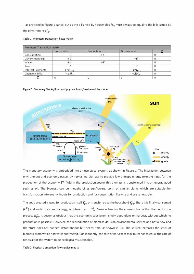
Table 1: Monetary transaction-flows matrix
Figure 1: Monetary Stocks/flows and physical funds/services of the model
The monetary economy is embedded into an ecological system, as shown in Figure 1. The interaction between
environment and economy occurs by harvesting biomass to provide low entropy energy (exergy) input for the
production of the economy 𝐸𝑝. Within the production sector this biomass is transformed into an energy good
such as oil. The biomass can be thought of as sunflowers, corn, or similar plants which are suitable for
transformation into energy inputs for production and for consumption likewise and are renewable.
The good created is used for production itself 𝑌𝑝𝑝𝑝 or transferred to the household 𝑌𝑝ℎ𝑝 . There it is finally consumed
(𝐶𝑝 ) and ends up as heat (anergy) on planet Earth 𝐻𝑝𝑒𝑝 . Same is true for the consumption within the production
process 𝐻𝑝𝑒𝑝 . It becomes obvious that the economic subsystem is fully dependent on harvest, without which no
production is possible. However, the reproduction of biomass 𝛥𝑆 is an environmental service and not a flow and
therefore does not happen instantaneous but needs time, as shown in 2.4. The service increases the stock of
biomass, from which harvest is subtracted. Consequently, the rate of harvest at maximum has to equal the rate of
renewal for the system to be ecologically sustainable.
Table 2: Physical transaction flow-service matrix
Monetary Transaction matrix
Households Production Government ∑
Consumption −𝐶 +𝐶 0 Government exp. +𝐺 −𝐺 0
Wages +𝑌 −𝑌 0
Taxes −𝑇 +𝑇 0 Interest Payments +𝑟𝑀𝑡−1 −𝑟𝑀𝑡−1 0
Change in bills −𝛥𝑀ℎ +𝛥𝑀𝑔 0 ∑ 0 0 0 0
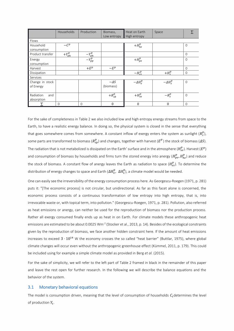
For the sake of completeness in Table 2 we also included low and high entropy energy streams from space to the
Earth, to have a realistic energy balance. In doing so, the physical system is closed in the sense that everything
that goes somewhere comes from somewhere. A constant inflow of exergy enters the system as sunlight (𝑅𝑠𝑝),
some parts are transformed to biomass (𝑅𝑠𝑝𝑝 ) and changes, together with harvest (𝐸𝑝 ) the stock of biomass (𝛥𝑆).
The radiation that is not metabolized is dissipated on the Earth’ surface and in the atmosphere (𝐻𝑠𝑒𝑝 ). Harvest (𝐸𝑝)
and consumption of biomass by households and firms turn the stored energy into anergy (𝐻𝑝𝑒𝑝 , 𝐻ℎ𝑒𝑝 ) and reduce
the stock of biomass. A constant flow of anergy leaves the Earth as radiation to space (𝐻𝑒𝑠𝑝 ). To determine the
distribution of energy changes to space and Earth (ΔHep, ΔHsp), a climate model would be needed.
One can easily see the irreversibility of the energy consumption process here. As Georgescu-Roegen (1971, p. 281)
puts it: "[The economic process] is not circular, but unidirectional. As far as this facet alone is concerned, the
economic process consists of a continuous transformation of low entropy into high entropy, that is, into
irrevocable waste or, with topical term, into pollution." (Georgescu-Roegen, 1971, p. 281). Pollution, also referred
as heat emissions or anergy, can neither be used for the reproduction of biomass nor the production process.
Rather all exergy consumed finally ends up as heat in on Earth. For climate models these anthropogenic heat
emissions are estimated to be about 0.0025 Wm-2 (Stocker et al., 2013, p. 14). Besides of the ecological constraints
given by the reproduction of biomass, we face another hidden constraint here. If the amount of heat emissions
increases to exceed 3 ⋅ 1014 W the economy crosses the so called “heat barrier” (Buttlar, 1975), where global
climate changes will occur even without the anthropogenic greenhouse effect (Kümmel, 2011, p. 179). This could
be included using for example a simple climate model as provided in Berg et al. (2015).
For the sake of simplicity, we will refer to the left part of Table 2 framed in black in the remainder of this paper
and leave the rest open for further research. In the following we will describe the balance equations and the
behavior of the system.
3.1 Monetary behavioral equations
The model is consumption driven, meaning that the level of consumption of households 𝐶𝑡determines the level
of production 𝑌𝑡.
Households Production Biomass, Low entropy
Heat on Earth High entropy
Space ∑
Flows
Household consumption
−𝐶𝑝 +𝐻ℎ𝑒𝑝 0
Product transfer +𝑌𝑝ℎ𝑝 −𝑌𝑝ℎ𝑝 0
Energy consumption
−𝑌𝑝𝑝𝑝 +𝐻𝑝𝑒𝑝 0
Harvest +𝐸𝑝 −𝐸𝑝 0 Dissipation −𝐻𝑒𝑠,𝑝 +𝐻𝑠𝑝 0
Services
Change in stock of Energy
−𝛥𝑆 (biomass)
−𝛥𝐻𝑒𝑝 −𝛥𝐻𝑠𝑝 0
Radiation and absorption
+𝑅𝑠𝑏𝑝 +𝐻𝑠𝑒𝑝 −𝑅𝑠𝑝 0 ∑ 0 0 0 0 0 0
𝑌𝑝ℎ,𝑡 = 𝐶𝑡 . (1)
To simplify the model, we assume that government expenditures 𝐺𝑡 = 𝐺 are constant over time and go directly
to the households. All earnings by the production sector 𝐶𝑡 are paid to households as wages. Capital is not included
in the model.
Additionally to wages, households receive income by interest payments with interest rate 𝑟 on bills 𝑀𝑡 from the
government sector. 𝑟 is assumed to be exogenously given and constant. Taxes with rate 𝜃 are paid on income, so
disposable income 𝑌𝐷,𝑡 and taxes 𝑇𝑡 are given by 𝑌𝐷,𝑡 = (1 − 𝜃)(𝐶𝑡 + 𝐺𝑡 + 𝑟𝑀𝑡), (2) 𝑇𝑡 = 𝜃(𝐶𝑡 + 𝐺𝑡 + 𝑟𝑀𝑡). (3)
The discrete equation of motion for the stock of bills (𝑀ℎand 𝑀𝑔that are identical) is given by 𝑀𝑡 = 𝑀𝑡−1 + 𝑌𝐷,𝑡 − 𝐶𝑡 . (4)
Bills of the previous period 𝑀𝑡−1 is increased by disposable income less realized consumption 𝐶𝑡. Note that
households have a consumption target 𝐶𝑡𝑇, which is different to realized consumption 𝐶𝑡. It is determined by the
propensity to consume out of disposable income of the last period (the first term) and out of wealth (the second
term)6 𝐶𝑡𝑇 = 𝑐𝑦(1 − 𝜃)(𝐶𝑡−1 + 𝐺𝑡−1 + 𝑟𝑀𝑡−1) + 𝑐𝑀𝑀𝑡−1. (5)
We differentiate between targeted and realized consumption 𝐶𝑡 because targeted consumption may be decreased
due to ecological constraints, which will be the focus of the physical equations (s. Equation (11)). For targeted
production, it follows 𝑌𝑝ℎ,𝑡𝑇 = 𝐶𝑡𝑇 . (6)
3.2 Physical flow equations
Before producers can produce anything, there must be a stock of biomass. We differ here from Heyes (2000) and
Lawn (2003) and assume that biomass is not growing exponentially if undisturbed, but as logistic growth. These
growth functions are very common in environmental modelling (Wainwright and Mulligan, 2013).
St = St−1 + St−1a (1 − St−1Smax) − Et with 0 < a < 2.6 (7)
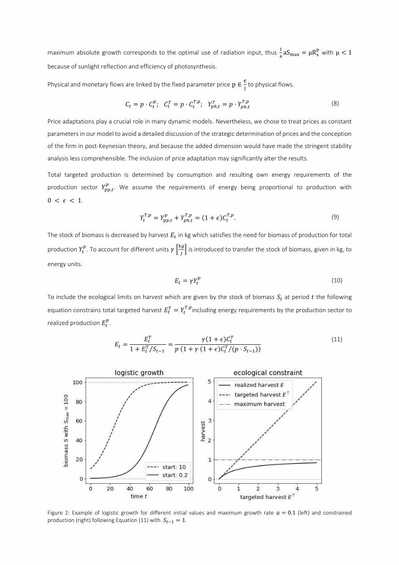
The growth function can be thought of as a S-curve, whereas the stock is limited to Smax. For small St−1 the stock
of the next period St does only increase exponentially, for St−1 = 12 Smax absolute growth is maximum with ΔS =14 aSmax to decline as St−1 approaches Smax, as shown in Figure 2. Thus the relation between the radiation turned
into biomass Rsbp = 𝑆𝑡−1𝑎 (1 − 𝑆𝑡−1𝑆𝑚𝑎𝑥) and the dissipation to heat on Earth Hsep is altered depending on the biomass
already available: In the desert, all radiation is turned to heat, as no radiation is transformed into biomass. The
6 Consumption out of interest payments is neglected to simplify the model
maximum absolute growth corresponds to the optimal use of radiation input, thus 14 aSmax = μRsp with μ < 1
because of sunlight reflection and efficiency of photosynthesis.
Physical and monetary flows are linked by the fixed parameter price p ∈ €J to physical flows.
𝐶𝑡 = 𝑝 ⋅ 𝐶𝑡𝑝; 𝐶𝑡𝑇 = 𝑝 ⋅ 𝐶𝑡𝑇,𝑝; 𝑌𝑝ℎ,𝑡𝑇 = 𝑝 ⋅ 𝑌𝑝ℎ,𝑡𝑇,𝑝 (8)
Price adaptations play a crucial role in many dynamic models. Nevertheless, we chose to treat prices as constant
parameters in our model to avoid a detailed discussion of the strategic determination of prices and the conception
of the firm in post-Keynesian theory, and because the added dimension would have made the stringent stability
analysis less comprehensible. The inclusion of price adaptation may significantly alter the results.
Total targeted production is determined by consumption and resulting own energy requirements of the
production sector 𝑌𝑝𝑝,𝑡𝑝 . We assume the requirements of energy being proportional to production with 0 < 𝜖 < 1. 𝑌𝑡𝑇,𝑝 = 𝑌𝑝𝑝,𝑡𝑝 + 𝑌𝑝ℎ,𝑡𝑇,𝑝 = (1 + 𝜖)𝐶𝑡𝑇,𝑝. (9)
The stock of biomass is decreased by harvest 𝐸𝑡 in kg which satisfies the need for biomass of production for total
production 𝑌𝑡𝑝. To account for different units 𝛾 [𝑘𝑔𝐽 ] is introduced to transfer the stock of biomass, given in kg, to
energy units. 𝐸𝑡 = 𝛾𝑌𝑡𝑝 (10)
To include the ecological limits on harvest which are given by the stock of biomass 𝑆𝑡 at period 𝑡 the following
equation constrains total targeted harvest 𝐸𝑡𝑇 = 𝑌𝑡𝑇,𝑝including energy requirements by the production sector to
realized production 𝐸𝑡𝑝.
𝐸𝑡 = 𝐸𝑡𝑇1 + 𝐸𝑡𝑇 𝑆𝑡−1⁄ = 𝛾(1 + 𝜖)𝐶𝑡𝑇𝑝 (1 + 𝛾 (1 + 𝜖)𝐶𝑡𝑇 (𝑝 ⋅ 𝑆𝑡−1)⁄ ) (11)
Figure 2: Example of logistic growth for different initial values and maximum growth rate 𝑎 = 0.1 (left) and constrained production (right) following Equation (11) with 𝑆𝑡−1 = 1.
The rationale behind Equation (11) is that if harvest is small compared to the stock of biomass (as is for example
the case for forestry in most countries), the realized harvest is close to identical to the desired one, to demand.
On the other hand, if targeted harvest is very high, the dynamical system has to guarantee that the harvest does
not exceed the available stock, which is impossible. This equation is an example how such a ‘smooth rationing’ in
the case of ecological scarcity can be implemented. Compared to a piecewise linear function, it avoids
discontinuities which would make the stability analysis much more challenging.
It follows for the realized physical consumption of households with Equation (8) is given by
𝐶𝑡𝑝 = 𝑌𝑡𝑝1 + 𝜖. (12)
3.3 System of equations
Accordingly, we can derive the equations that determine the behavior of the system. To simplify the notation, we
use the relation 𝛾𝜖 = (1 + 𝜖)𝛾 and 𝑌𝑡𝑝 = 𝑌𝑡,𝜖𝑝1+𝜖. 𝑌𝑡𝑝 differs from 𝑌𝑡,𝜖𝑝 by not including internal energy consumption of
production.
𝑌𝑡𝑝 = 𝐶𝑡𝑇𝑝 + 𝛾𝜖𝐶𝑡𝑇 𝑆𝑡−1⁄ (13)
𝑆𝑡 = 𝑆𝑡−1 + 𝑆𝑡−1𝑎 (1 − 𝑆𝑡−1𝑆𝑚𝑎𝑥) − 𝛾𝜖𝑌𝑡𝑝𝑤𝑖𝑡ℎ0 < 𝑎 < 2.6 (14)
𝑀𝑡 = 𝑀𝑡−1 + (1 − 𝜃)(𝐺0 + 𝑟𝑀𝑡−1) − 𝜃𝑌𝑡𝑝𝑝 (15)
With 𝐶𝑡𝑇 = 𝑐𝑦(1 − 𝜃)(𝑝𝑌𝑡−1𝑝 + 𝐺0 + 𝑟𝑀𝑡−1) + 𝑐𝑀𝑀𝑡−1 (16) 𝑌𝑡,𝜖𝑝 = 𝑌𝑡𝑝(1 + 𝜖) (17)
It is a three-dimensional system depended on 𝑀𝑡 , 𝑌𝑡𝑝and 𝑆𝑡 which determines the behavior of the system.
Equations (16) and (17) are only substitutes for the values of 𝐶𝑡𝑇 and 𝑌𝑡,𝜖𝑝 , so the system remains three-dimensional.
For the simulation, one has to know the initial values of 𝑌0𝑝, 𝑀0 and 𝑆0. With these initial conditions we can
calculate 𝐶𝑡𝑇 according to Equation (16) by using values known from the previous period 𝐶𝑡−1 and 𝑀𝑡−1. The result
is substituted into 𝑌𝑡𝑝 from Equation (13) which goes into 𝑆𝑡 via Equation (14) and 𝑀𝑡 via Equation (15). This
procedure is repeated for as many time steps as preferred.
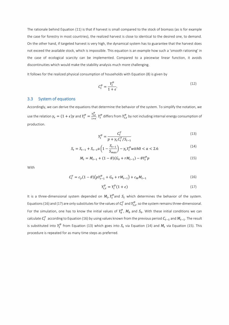
4 Simulation results of the model To give a first intuition of the model behavior, we obtained simulation results for the model with Python. From
these, we can derive three different kinds of model behavior, represented in Figure 3. The left graph shows an
ecologically and monetarily stable system that converges towards a stationary state for 𝑀, 𝑆, and 𝑌. In this case
economically driven harvest and ecologically driven reproduction are equal leading to an ecological stability.
Furthermore, the system is monetarily stable, due to high levels of consumption out of wealth compared to the
interest rate. We will give a detailed explanation of this behavior in Section 5. In the middle graph, the system
tends to a monetarily stable stationary state, indicated by the concave shape of 𝑀 and 𝑌. However, as one can
see from the monotonically declining course of 𝑆 the ecological system is continuously overused leading to an
ecological collapse at 𝑡 = 360 causing an immediate economic collapse. However, since the government
continues to pay interests on bills the monetary stock continuously increases. A more drastic result is obtained in
the ‘explosive’ right graph of Figure 3. Due to high interest rates compared to consumption out of wealth, the
system is monetarily unstable and grows out of bound, indicated by the convex shape of 𝑀. As the economy
cannot grow forever due to ecological constraints, it collapses at 𝑡 = 150 – just like in the middle graph – because
it continuously overuses the ecology. Note that in this scenario, the government debt to GDP ratio increases
unlimitedly even before the ecological collapse – thus we don’t see stable growth but rather a debt spiral where
the consumptive government expenditures become negligible compared to debt services, not indicating economic
stability. Furthermore, the model abstracts from expectations that might cause negative output effects due to
high debt to GDP ratios.
Figure 3: Time evolution of the system for different propensities to consume out of wealth. Parameters 𝜃 = 0.5, 𝑐𝑦 = 0.8, 𝑎 =0.1, 𝑝 = 4, 𝛾 = 1.1, 𝑆𝑚𝑎𝑥 = 100, 𝐺 = 4, 𝑟 = 0.1 and initial values 𝑆0 = 100, 𝑌0𝑝 = 1, 𝑌0 = 𝑝𝑌0𝑝 = 4,𝑀0 = 10. Left graph: monetarily and ecologically stable system with 𝑐𝑚 = 0.06. Center: monetarily stable, but ecologically unstable economy with 𝑐𝑚 = 0.04. Right graph: monetarily and ecologically unstable ‘explosive’ system with 𝑐𝑚 = 0.01.
5 Stability Analysis of the model To analyze the model, explain the differences pictured in Figure 3 and derive more insights in its general behavior,
we conducted a stability analysis of the three-dimensional system.7 For the calculation of fixed points, where no
change in either variable occurs, we must state that 𝑆𝑡 = 𝑆𝑡−1; 𝑀𝑡 = 𝑀𝑡−1; 𝑌𝑡𝑝 = 𝑌𝑡−1𝑝 . (18)
In doing so, we can derive the coordinates of the fixed points (see Appendix A). The stationary state for the biomass
stock 𝑆∗ is the closed form solution of the cubic equation
𝑎𝛾𝜖 𝑆∗ (1 − 𝑆∗𝑆𝑚𝑎𝑥)( 11 − 𝑎 (1 − 𝑆∗𝑆𝑚𝑎𝑥) − 𝑐𝑦 − 𝑐𝑚𝜃(1 − 𝜃)𝑟)⏟ 𝐹(𝑆)= −𝑐𝑚𝑟𝑝 𝐺. (19)
Reasonable results can be obtained for 𝑆∗ ∈ [0, 𝑆𝑚𝑎𝑥], whereby the equation is solvable for 𝑟 ≠ 0; 𝜃 ≠ 1; 𝑝 ≠0; 𝑎 ≠ 1; 𝛾𝜖 ≠ 0. Knowing 𝑆∗ we can calculate the stationary states of production 𝑌𝑝∗ and the stock of bills 𝑀∗ with
𝑌𝑝∗ = 𝑎𝛾𝜖 𝑆∗ (1 − 𝑆∗𝑆𝑚𝑎𝑥),
(20)
𝑀∗ = 𝜃𝑝𝑌𝑝∗ − (1 − 𝜃)𝐺1 − 𝜃𝑟 . (21)
From Equations (19) to (21) we can conclude, that the number of fixed points depends solely on the number of
solutions for Equation (19). Since by definition S∗ ∈ [0, 𝑆𝑚𝑎𝑥] we can state further, that no solution exists and
accordingly, there will be no stationary state within this domain, if 𝐹(𝑆∗) > 0. In this case, the stock of biomass 𝑆∗ < 0 or 𝑆∗ > 𝑆𝑚𝑎𝑥 . We can interpret this result as a global instability, which leads to over-depletion of the
biomass stock and consequently to the collapse of the ecological system. As shown in Appendix B 𝐹(𝑆∗) > 0 for
any 𝑆∗ ∈ [0, 𝑆𝑚𝑎𝑥]if 𝑐𝑟 = 𝑐𝑚𝑟 < (1 − 𝑐𝑦)(1 − 𝜃)𝜃 . (22)
This result is equal to the relation derived for the SIM model of Godley and Lavoie (2012) by Richters and Siemoneit
(2017). However, in contrast to this paper, they do not consider ecological variables. Note, that this relation is
independent of the biomass growth rate 𝑎. Therefore, it can be interpreted as the monetary stability condition. If
Inequality (22 is fulfilled, consumption and production will increase unboundedly which necessarily leads to an
ecological collapse at some point in time in our model, even for very high ecological regeneration. However, it is
possible to have positive interest rates within a monetarily stable economy. In this case, positive interest rates
7 For general information on stability analysis see Argyris et al. (2015). An application to stock-flow
consistent models is provided by Richters and Siemoneit (2017).
have a positive effect on the stock of government bills of the economy, as they determine the speed of the
accumulation of bills. If the dampening effect by consumption out of wealth 𝑐𝑚 is high compared to the interest
rate 𝑟 the economy becomes stable (compare Figure 1).
To analyze the conditions for stability dependent on changes on certain parameters, as for example the ratio 𝑐𝑟of 𝑐𝑚 and 𝑟, we can convert Equation (19) to an implicit function as follows:
𝐾(𝑆∗, 𝑐𝑟) ≔ 𝑎𝛾𝜖 𝑆∗ (1 − 𝑆∗𝑆𝑚𝑎𝑥)( 11 − 𝑎 (1 − 𝑆∗𝑆𝑚𝑎𝑥) − 𝑐𝑦 − 𝑐𝑟𝜃(1 − 𝜃)) + 𝑐𝑟𝑝 𝐺 = 0. (23)
We can now picture the solutions for Equation (19) for different values of 𝑐𝑟 by plotting the implicit function of
Equation (47), as shown in the bifurcation diagram in Figure 4.
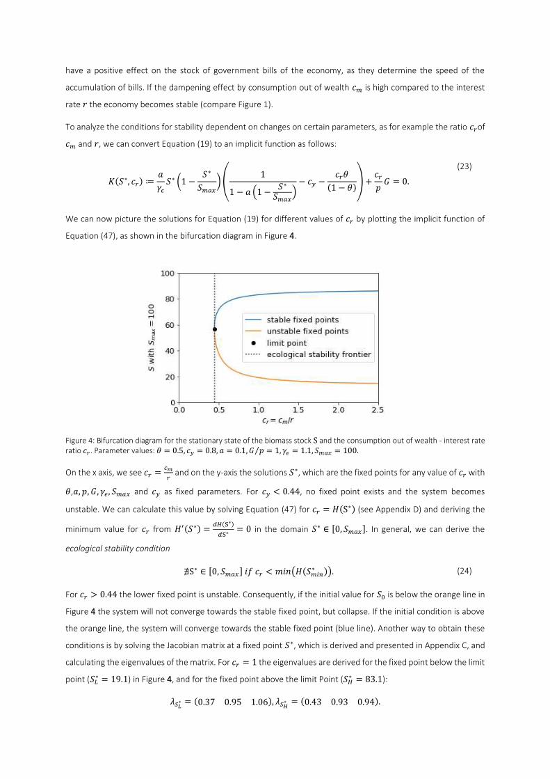
Figure 4: Bifurcation diagram for the stationary state of the biomass stock S and the consumption out of wealth - interest rate ratio 𝑐𝑟. Parameter values: 𝜃 = 0.5, 𝑐𝑦 = 0.8, 𝑎 = 0.1, 𝐺 𝑝⁄ = 1, 𝛾𝜖 = 1.1, 𝑆𝑚𝑎𝑥 = 100. On the x axis, we see 𝑐𝑟 = 𝑐𝑚𝑟 and on the y-axis the solutions 𝑆∗, which are the fixed points for any value of 𝑐𝑟 with 𝜃,𝑎, 𝑝, 𝐺, 𝛾𝜖, 𝑆𝑚𝑎𝑥 and 𝑐𝑦 as fixed parameters. For 𝑐𝑦 < 0.44, no fixed point exists and the system becomes
unstable. We can calculate this value by solving Equation (47) for 𝑐𝑟 = 𝐻(S∗) (see Appendix D) and deriving the
minimum value for 𝑐𝑟 from 𝐻′(𝑆∗) = 𝑑𝐻(S∗)𝑑S∗ = 0 in the domain 𝑆∗ ∈ [0, 𝑆𝑚𝑎𝑥]. In general, we can derive the
ecological stability condition ∄S∗ ∈ [0, 𝑆𝑚𝑎𝑥] 𝑖𝑓 𝑐𝑟 < 𝑚𝑖𝑛(𝐻(𝑆𝑚𝑖𝑛∗ )). (24)
For 𝑐𝑟 > 0.44 the lower fixed point is unstable. Consequently, if the initial value for 𝑆0 is below the orange line in
Figure 4 the system will not converge towards the stable fixed point, but collapse. If the initial condition is above
the orange line, the system will converge towards the stable fixed point (blue line). Another way to obtain these
conditions is by solving the Jacobian matrix at a fixed point 𝑆∗, which is derived and presented in Appendix C, and
calculating the eigenvalues of the matrix. For 𝑐𝑟 = 1 the eigenvalues are derived for the fixed point below the limit
point (𝑆𝐿∗ = 19.1) in Figure 4, and for the fixed point above the limit Point (𝑆𝐻∗ = 83.1): 𝜆𝑆𝐿∗ = (0.37 0.95 1.06), 𝜆𝑆𝐻∗ = (0.43 0.93 0.94).
Since one of the eigenvalues of 𝑆𝐿∗ is higher than one, this fixed point is unstable. For 𝑆𝐻∗ all eigenvalues are lower
than one, consequently this fixed point is stable and the system will converge to it.
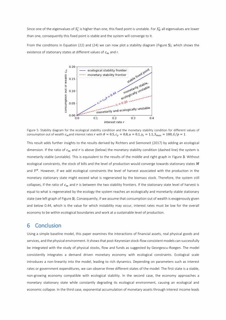
From the conditions in Equation (22) and (24) we can now plot a stability diagram (Figure 5), which shows the
existence of stationary states at different values of 𝑐𝑚 and r.
Figure 5: Stability diagram for the ecological stability condition and the monetary stability condition for different values of consumption out of wealth 𝑐𝑚and interest rates 𝑟 with 𝜃 = 0.5, 𝑐𝑦 = 0.8, 𝑎 = 0.1, 𝛾𝜖 = 1.1, 𝑆𝑚𝑎𝑥 = 100, 𝐺 𝑝⁄ = 1.
This result adds further insights to the results derived by Richters and Siemoneit (2017) by adding an ecological
dimension. If the ratio of 𝑐𝑚 and 𝑟 is above (below) the monetary stability condition (dashed line) the system is
monetarily stable (unstable). This is equivalent to the results of the middle and right graph in Figure 3. Without
ecological constraints, the stock of bills and the level of production would converge towards stationary states 𝑀
and 𝑌𝑝. However, if we add ecological constraints the level of harvest associated with the production in the
monetary stationary state might exceed what is regenerated by the biomass stock. Therefore, the system still
collapses, if the ratio of 𝑐𝑚 and 𝑟 is between the two stability frontiers. If the stationary state level of harvest is
equal to what is regenerated by the ecology the system reaches an ecologically and monetarily stable stationary
state (see left graph of Figure 3). Consequently, if we assume that consumption out of wealth is exogenously given
and below 0.44, which is the value for which instability may occur, interest rates must be low for the overall
economy to be within ecological boundaries and work at a sustainable level of production.
6 Conclusion Using a simple baseline model, this paper examines the interactions of financial assets, real physical goods and
services, and the physical environment. It shows that post-Keynesian stock-flow consistent models can successfully
be integrated with the study of physical stocks, flow and funds as suggested by Georgescu-Roegen. The model
consistently integrates a demand driven monetary economy with ecological constraints. Ecological scale
introduces a non-linearity into the model, leading to rich dynamics. Depending on parameters such as interest
rates or government expenditures, we can observe three different states of the model: The first state is a stable,
non-growing economy compatible with ecological stability. In the second case, the economy approaches a
monetary stationary state while constantly degrading its ecological environment, causing an ecological and
economic collapse. In the third case, exponential accumulation of monetary assets through interest income leads
to ever increasing demand, ecological degradation and finally breakdown. One major factor driving these
differences is the parameter ratio of consumption out of wealth and interest rate. If consumption out of wealth is
low, low interest rates are needed for the model to converge towards a sustainable stationary state of production.
The (relative) simplicity of the model makes it tractable and easier to analyze, while obviously neglecting several
important aspects such as multiple goods, pricing, fixed capital, income distribution, complex financial assets or
portfolio choice. Restricting our depiction to energy, even a treatment of physical mass, waste or carbon emissions
is missing as provided by Taylor et al. (2016) or Dafermos et al. (2017). The integration of these concepts can
profit from a growing literature in post-Keynesian and ecological economics. Combining both approaches and
integrating monetary and ecological issues may be helpful to determine the conditions under which a sustainable
economy is possible, a problem that is neither purely economic, nor purely environmental, nor purely physical,
but rather are all of the above.
i
7 References Argyris, J.H., Faust, G. and Haase, M. (2015), An Exploration of Dynamical Systems and Chaos: Completely Revised
and Enlarged Second Edition, Springer Berlin Heidelberg, Berlin Heidelberg.
Berg, M., Hartley, B. and Richters, O. (2015), “A stock-flow consistent input–output model with applications to
energy price shocks, interest rates, and heat emissions”, New Journal of Physics, Vol. 17 No. 1, p. 15011.
Bezemer, D.J. (2010), “Understanding financial crisis through accounting models”, Accounting, Organizations and
Society, Vol. 35 No. 7, pp. 676–688.
Buttlar, H.v. (1975), “Umweltprobleme”, Physikalische Blätter, Vol. 31 No. 4, pp. 145–155.
Dafermos, Y., Nikolaidi, M. and Galanis, G. (2017), “A stock-flow-fund ecological macroeconomic model”,
Ecological Economics, Vol. 131, pp. 191–207.
Dale, M., Krumdieck, S. and Bodger, P.S. (2012), “Global energy modelling — A biophysical approach (GEMBA)
Part 1: An overview of biophysical economics”, Ecological Economics, Vol. 73, pp. 152–157.
Daly, H.E. (1985), “The Circular Flow of Exchange Value and the Linear Throughput of Matter-Energy: A Case of
Misplaced Concreteness”, Review of Social Economy, Vol. 43 No. 3, pp. 279–297.
Daly, H.E. (1992), “Allocation, distribution, and scale: towards an economics that is efficient, just, and
sustainable”, Ecological Economics, Vol. 6 No. 3, pp. 185–193.
Dobusch, L. and Kapeller, J. (2012), “Heterodox united vs. mainstream city? Sketching a framework for interested
pluralism in economics”, Journal of Economic Issues, Vol. 46 No. 4, pp. 1035–1058.
Galbraith, J.K. (2009), “Amen”, Thought & Action, pp. 85–97.
Georgescu-Roegen, N. (1971), The Entropy Law and the Economic Process, Harvard University Press, Cambridge,
Mass.
Godley, W. and Lavoie, M. (2012), Monetary economics: an integrated approach to credit, money, income,
production and wealth, 2nd ed., Palgrave Macmillan, Basingstoke, New York.
Gowdy, J.M. (1991), “Bioeconomics and post Keynesian economics: a search for common ground”, Ecological
Economics, Vol. 3 No. 1, pp. 77–87.
Heyes, A. (2000), “A proposal for the greening of textbook macro: ‘IS-LM-EE’”, Ecological Economics, Vol. 32
No. 1, pp. 1–7.
Holt, R.P.F., Pressman, S. and Spash, C. (Eds.) (2009), Post Keynesian and Ecological Economics: Confronting
Environmental Issues, Edward Elgar, Cheltenham, U.K.
Keynes, J.M. (1936), The general theory of employment, interest and money, Harcourt, Brace, New York.
Koo, R. (2011), “The world in balance sheet recession: causes, cure, and politics”, Real-world economics review,
Vol. 58 No. 12, pp. 19–37.
Kronenberg, T. (2010), “Finding common ground between ecological economics and post-Keynesian economics”,
Ecological Economics, Vol. 69 No. 7, pp. 1488–1494.
Kümmel, R. (2011), The Second Law of Economics: Energy, Entropy, and the Origins of Wealth, Springer, New
York, Dordrecht, Heidelberg, London.
Lavoie, M. (2006), “Do Heterodox Theories Have Anything in Common? A Post-Keynesian Point of View”,
European Journal of Economics and Economic Policies: Intervention, Vol. 3 No. 1, pp. 87–112.
Lawn, P.A. (2003), “On Heyes’ IS–LM–EE proposal to establish an environmental macroeconomics”, Environment
and Development Economics, Vol. 8 No. 01, pp. 31–56.
Ott, K. and Döring, R. (2008), Theorie und Praxis starker Nachhaltigkeit, Beiträge zur Theorie und Praxis starker
Nachhaltigkeit, Bd. 1, 2nd ed., Metropolis, Marburg.
Perman, R. (2011), Natural resource and environmental economics, 4. ed., Pearson Education Limited, Harlow,
Munich.
Rezai, A. and Stagl, S. (2016), “Ecological macroeconomics: Introduction and review”, Ecological Economics,
Vol. 121, pp. 181–185.
Richters, O. and Siemoneit, A. (2017), “Consistency and stability analysis of models of a monetary growth
imperative”, Ecological Economics, Vol. 136, pp. 114–125.
Rockström, J., Steffen, W., Noone, K., Persson, Å., Chapin, F.S., Lambin, E.F., Lenton, T.M., Scheffer, M., Folke, C.,
Schellnhuber, H.J., Nykvist, B., Wit, C.A. de, Hughes, T., van der Leeuw, S., Rodhe, H., Sörlin, S., Snyder, P.K.,
Costanza, R., Svedin, U., Falkenmark, M., Karlberg, L., Corell, R.W., Fabry, V.J., Hansen, J., Walker, B.,
Liverman, D., Richardson, K., Crutzen, P. and Foley, J.A. (2009), “A safe operating space for humanity”,
Nature, Vol. 461 No. 7263, pp. 472–475.
Stocker, T.F., Qin, D., Plattner, G.K., Tignor, M., Allen, S.K., Boschung, J., Nauels, A., Xia, Y., Bex, V. and Midgley,
P.M. (Eds.) (2013), Climate Change 2013: The Physical Science Basis. Contribution of Working Group I to the
Fifth Assessment Report of the Intergovernmental Panel on Climate Change, Cambridge University Press,
Cambridge, U.K.
Taylor, L., Rezai, A. and Foley, D.K. (2016), “An integrated approach to climate change, income distribution,
employment, and economic growth”, Ecological Economics, Vol. 121, pp. 196–205.
Wainwright, J. and Mulligan, M. (2013), Environmental modelling: Finding simplicity in complexity, 2nd edition,
Wiley-Blackwell, Chichester.
WCED (1987), Our common future, Oxford University Press, Oxford, New York.
Appendix
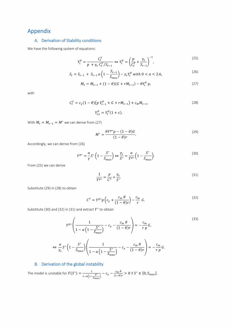
A. Derivation of Stability conditions
We have the following system of equations:
𝑌𝑡𝑝 = 𝐶𝑡𝑇𝑝 + 𝛾𝜖 𝐶𝑡𝑇 𝑆𝑡−1⁄ ⇔ 𝑌𝑡𝑝 = ( 𝑝𝐶𝑡𝑇 + 𝛾𝜖𝑆𝑡−1)−1, (25)
𝑆𝑡 = 𝑆𝑡−1 + 𝑆𝑡−1 𝑎 (1 − 𝑆𝑡−1𝑆𝑚𝑎𝑥) − 𝛾𝜖𝑌𝑡𝑝 𝑤𝑖𝑡ℎ 0 < 𝑎 < 2.6, (26)
𝑀𝑡 = 𝑀𝑡−1 + (1 − 𝜃)(𝐺 + 𝑟𝑀𝑡−1) − 𝜃𝑌𝑡𝑝 𝑝, (27)
with 𝐶𝑡𝑇 = 𝑐𝑦(1 − 𝜃)(𝑝 𝑌𝑡−1𝑝 + 𝐺 + 𝑟𝑀𝑡−1) + 𝑐𝑀𝑀𝑡−1, 𝑌𝑡,𝜖𝑝 = 𝑌𝑡𝑝(1 + 𝜖). (28)
With 𝑀𝑡 = 𝑀𝑡−1 = 𝑀∗ we can derive from (27)
𝑀∗ = 𝜃𝑌𝑝∗𝑝 − (1 − 𝜃)𝐺(1 − 𝜃)𝑟 . (29)
Accordingly, we can derive from (26)
𝑌𝑝∗ = 𝑎𝛾 𝑆∗ (1 − 𝑆∗𝑆𝑚𝑎𝑥) ⇔ 𝛾𝜖𝑆∗ = 𝑎𝑌𝑝∗ (1 − 𝑆∗𝑆𝑚𝑎𝑥). (30)
From (25) we can derive 1𝑌𝑝∗ = 𝑝𝐶𝑇 + 𝛾𝜖𝑆∗. (31)
Substitute (29) in (28) to obtain
𝐶𝑇 = 𝑌𝑝∗𝑝 (𝑐𝑦 + 𝑐𝑚 𝜃(1 − 𝜃)𝑟) − 𝑐𝑚𝑟 𝐺. (32)
Substitute (30) and (32) in (31) and extract 𝑌∗ to obtain
𝑌𝑝∗( 11 − 𝑎 (1 − 𝑆∗𝑆𝑚𝑎𝑥) − 𝑐𝑦 − 𝑐𝑚 𝜃(1 − 𝜃)𝑟) = − 𝑐𝑚𝑟 𝑝 𝐺, ⇔ 𝑎𝛾𝜖 𝑆∗ (1 − 𝑆∗𝑆𝑚𝑎𝑥)( 11 − 𝑎 (1 − 𝑆∗𝑆𝑚𝑎𝑥) − 𝑐𝑦 − 𝑐𝑚 𝜃(1 − 𝜃)𝑟) = − 𝑐𝑚𝑟 𝑝 𝐺.
(33)
B. Derivation of the global instability
The model is unstable for 𝐹(𝑆∗) = 11−𝑎(1− 𝑆∗𝑆𝑚𝑎𝑥)− 𝑐𝑦 − 𝑐𝑚 𝜃(1−𝜃)𝑟 > 0 if 𝑆∗ ∈ [0, 𝑆𝑚𝑎𝑥].
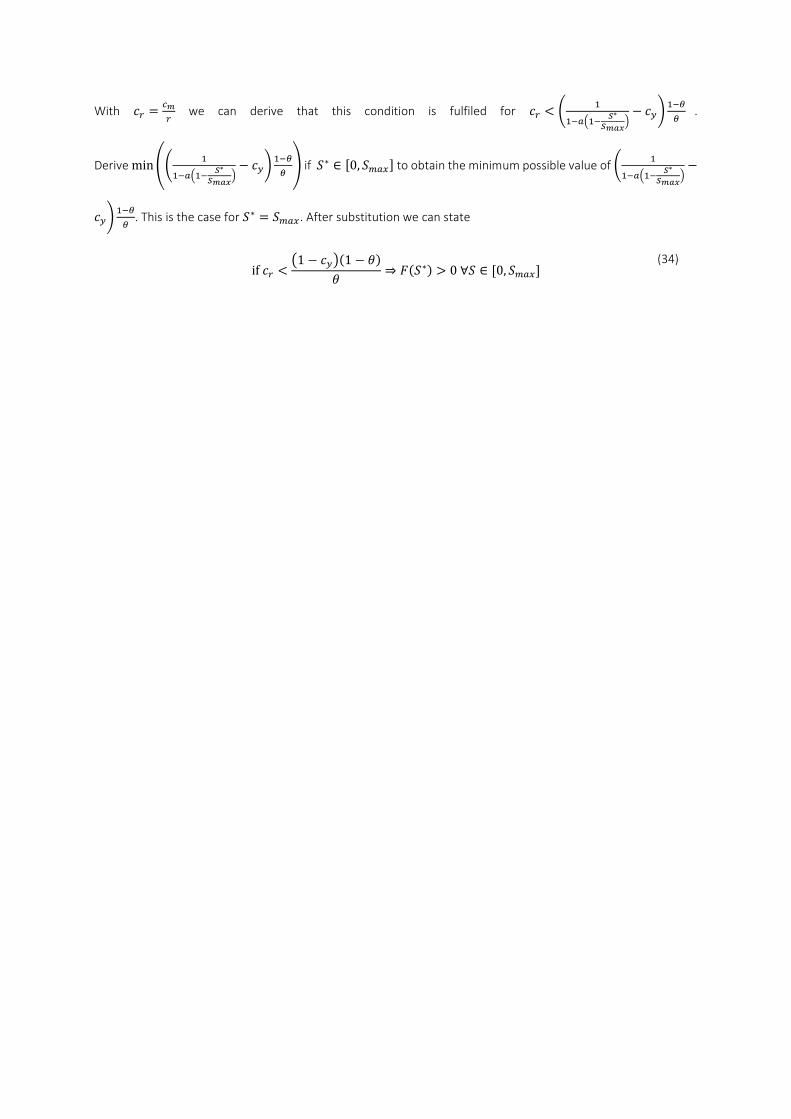
With 𝑐𝑟 = 𝑐𝑚𝑟 we can derive that this condition is fulfiled for 𝑐𝑟 < ( 11−𝑎(1− 𝑆∗𝑆𝑚𝑎𝑥)− 𝑐𝑦) 1−𝜃𝜃 . Derive min(( 11−𝑎(1− 𝑆∗𝑆𝑚𝑎𝑥)− 𝑐𝑦) 1−𝜃𝜃 ) if 𝑆∗ ∈ [0, 𝑆𝑚𝑎𝑥] to obtain the minimum possible value of ( 11−𝑎(1− 𝑆∗𝑆𝑚𝑎𝑥)−𝑐𝑦) 1−𝜃𝜃 . This is the case for 𝑆∗ = 𝑆𝑚𝑎𝑥. After substitution we can state
if 𝑐𝑟 < (1 − 𝑐𝑦)(1 − 𝜃)𝜃 ⇒ 𝐹(𝑆∗) > 0 ∀𝑆 ∈ [0, 𝑆𝑚𝑎𝑥] (34)
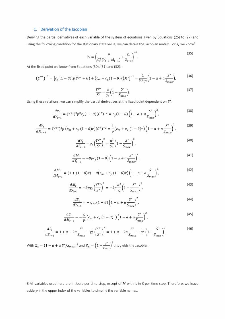
C. Derivation of the Jacobian
Deriving the partial derivatives of each variable of the system of equations given by Equations (25) to (27) and
using the following condition for the stationary state value, we can derive the Jacobian matrix. For 𝑌𝑡 we know8
𝑌𝑡 = ( 𝑝𝐶𝑡𝑇(𝑌𝑡−1, 𝑀𝑡−1) + 𝛾𝜖𝑆𝑡−1)−1. (35)
At the fixed point we know from Equations (30), (31) and (32):
(𝐶𝑇∗)−1 = [𝑐𝑦 (1 − 𝜃)(𝑝 𝑌𝑝∗ + 𝐺) + (𝑐𝑚 + 𝑐𝑦(1 − 𝜃)𝑟)𝑀∗]−1 = 1𝑌𝑝∗𝑝 (1 − 𝑎 + 𝑎 𝑆∗𝑆𝑚𝑎𝑥), (36)
𝑌𝑝∗𝑆∗ = 𝑎𝛾𝜖 (1 − 𝑆∗𝑆𝑚𝑎𝑥 ). (37)
Using these relations, we can simplify the partial derivatives at the fixed point dependent on 𝑆∗: 𝑑𝑌𝑡𝑑𝑌𝑡−1 = (𝑌𝑝∗)2𝑝2𝑐𝑦(1 − 𝜃)(𝐶𝑇)−2 = 𝑐𝑦(1 − 𝜃) (1 − 𝑎 + 𝑎 𝑆∗𝑆𝑚𝑎𝑥)2, (38)
𝑑𝑌𝑡𝑑𝑀𝑡−1 = (𝑌𝑝∗)2𝑝 (𝑐𝑚 + 𝑐𝑦 (1 − 𝜃)𝑟)(𝐶𝑇)−2 = 1𝑝 (𝑐𝑚 + 𝑐𝑦 (1 − 𝜃)𝑟) (1 − 𝑎 + 𝑎 𝑆∗𝑆𝑚𝑎𝑥)2, (39)
𝑑𝑌𝑡𝑑𝑆𝑡−1 = 𝛾𝜖 (𝑌𝑝∗𝑆∗ )2 = 𝑎2𝛾𝜖 (1 − 𝑆∗𝑆𝑚𝑎𝑥 )2, (40)
𝑑𝑀𝑡𝑑𝑌𝑡−1 = −𝜃𝑝𝑐𝑦(1 − 𝜃) (1 − 𝑎 + 𝑎 𝑆∗𝑆𝑚𝑎𝑥)2, (41)
𝑑𝑀𝑡𝑑𝑀𝑡−1 = (1 + (1 − 𝜃)𝑟) − 𝜃(𝑐𝑚 + 𝑐𝑦 (1 − 𝜃)𝑟) (1 − 𝑎 + 𝑎 𝑆∗𝑆𝑚𝑎𝑥)2, (42)
𝑑𝑀𝑡𝑑𝑆𝑡−1 = −𝜃𝑝𝛾𝜖 (𝑌𝑝∗𝑆∗ )2 = −𝜃𝑝 𝑎2𝛾𝜖 (1 − 𝑆∗𝑆𝑚𝑎𝑥 )2, (43)
𝑑𝑆𝑡𝑑𝑌𝑡−1 = −𝛾𝜖𝑐𝑦(1 − 𝜃) (1 − 𝑎 + 𝑎 𝑆∗𝑆𝑚𝑎𝑥)2, (44)
𝑑𝑆𝑡𝑑𝑀𝑡−1 = −𝛾𝜖𝑝 (𝑐𝑚 + 𝑐𝑦 (1 − 𝜃)𝑟) (1 − 𝑎 + 𝑎 𝑆∗𝑆𝑚𝑎𝑥)2, (45)
𝑑𝑆𝑡𝑑𝑆𝑡−1 = 1 + 𝑎 − 2𝑎 𝑆∗𝑆𝑚𝑎𝑥 − 𝛾𝜖2 (𝑌𝑝∗𝑆∗ )2 = 1 + 𝑎 − 2𝑎 𝑆∗𝑆𝑚𝑎𝑥 − 𝑎2 (1 − 𝑆∗𝑆𝑚𝑎𝑥 )2. (46)
With 𝑍𝐴 = (1 − 𝑎 + 𝑎 𝑆∗/𝑆𝑚𝑎𝑥)2 and 𝑍𝐵 = (1 − 𝑆∗𝑆𝑚𝑎𝑥)2this yields the Jacobian
8 All variables used here are in Joule per time step, except of 𝑀 with is in € per time step. Therefore, we leave
aside 𝑝 in the upper index of the variables to simplify the variable names.
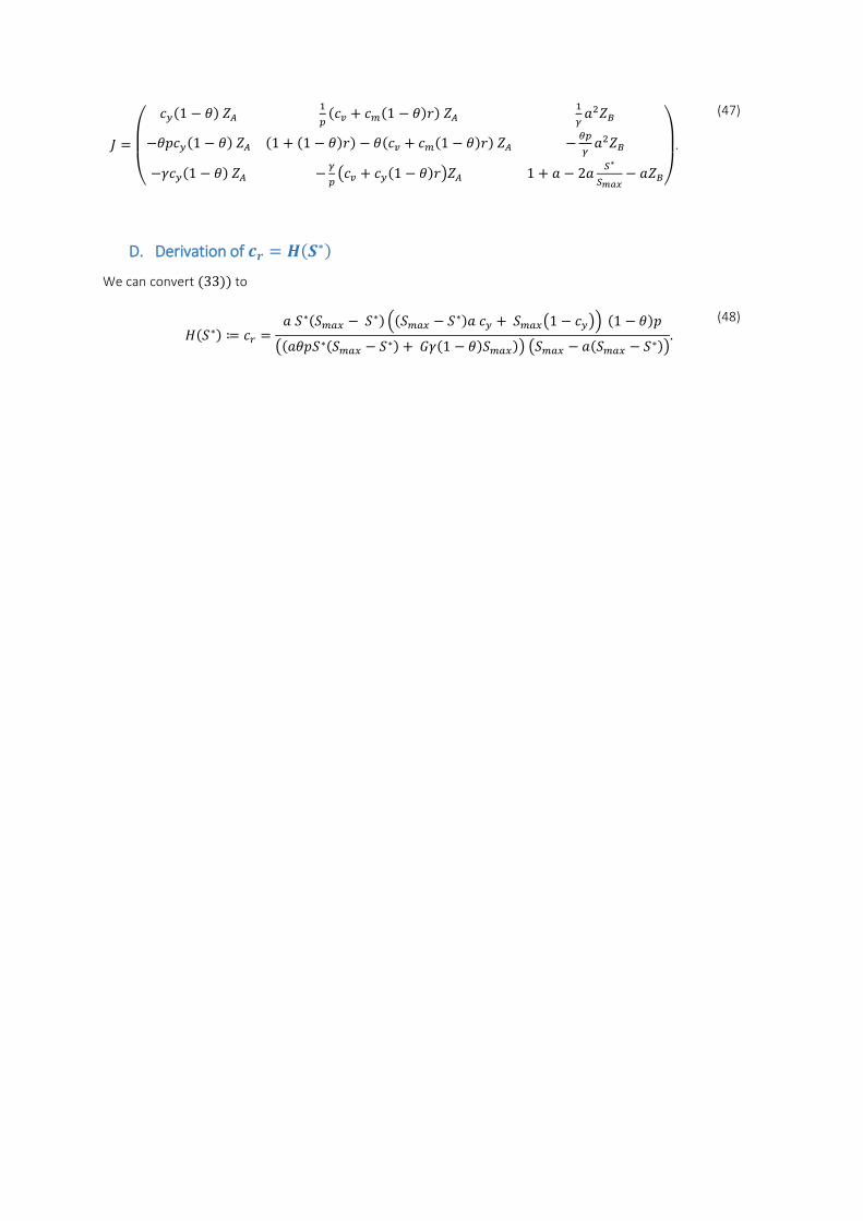
𝐽 = ( 𝑐𝑦(1 − 𝜃) 𝑍𝐴 1𝑝 (𝑐𝑣 + 𝑐𝑚(1 − 𝜃)𝑟) 𝑍𝐴 1𝛾 𝑎2𝑍𝐵−𝜃𝑝𝑐𝑦(1 − 𝜃) 𝑍𝐴 (1 + (1 − 𝜃)𝑟) − 𝜃(𝑐𝑣 + 𝑐𝑚(1 − 𝜃)𝑟) 𝑍𝐴 − 𝜃𝑝𝛾 𝑎2𝑍𝐵−𝛾𝑐𝑦(1 − 𝜃) 𝑍𝐴 − 𝛾𝑝 (𝑐𝑣 + 𝑐𝑦(1 − 𝜃)𝑟)𝑍𝐴 1 + 𝑎 − 2𝑎 𝑆∗𝑆𝑚𝑎𝑥 − 𝑎𝑍𝐵)
.
(47)
D. Derivation of 𝒄𝒓 = 𝑯(𝑺∗) We can convert (33)) to
𝐻(𝑆∗) ≔ 𝑐𝑟 = 𝑎 𝑆∗(𝑆𝑚𝑎𝑥 − 𝑆∗) ((𝑆𝑚𝑎𝑥 − 𝑆∗)𝑎 𝑐𝑦 + 𝑆𝑚𝑎𝑥(1 − 𝑐𝑦)) (1 − 𝜃)𝑝((𝑎𝜃𝑝𝑆∗(𝑆𝑚𝑎𝑥 − 𝑆∗) + 𝐺𝛾(1 − 𝜃)𝑆𝑚𝑎𝑥)) (𝑆𝑚𝑎𝑥 − 𝑎(𝑆𝑚𝑎𝑥 − 𝑆∗)). (48)
Recommended


![Detoxification Efforts in Longnose Dace …ble to population collapse by endocrine disruption than longer-lived fish [22]. Ecological consequences of con-taminant exposure vary extensively](https://img.pdfslide.net/doc/110x75/5ec2a65d00b5032f8366b306/detoxification-efforts-in-longnose-dace-ble-to-population-collapse-by-endocrine.jpg)