Design and Evaluation of Potential Cooling Cycles for the Reduction of Water Use in
Thermoelectric Power Plants
Thesis
By
Rhys Davis
Undergraduate Honors Program in Mechanical Engineering
The Ohio State University
2017
Thesis Committee:
Dr. Shaurya Prakash, Adviser
Dr. Bhavik Bakshi
Submitted to
The Engineering Honors Committee
119 Hitchcock Hall
College of Engineering
The Ohio State University
Columbus, Ohio 43210

ii
Abstract In the U.S., water for thermoelectric power plant cooling constitutes 40% of all
freshwater withdrawal and 4% of all freshwater consumption. There are two main kinds of
power plant cooling systems, once-through and recirculating, but environmental issues arise
from both types, including excessive water consumption and ecological damage from high
temperature return water. The purpose of this study is to identify effective while environmentally
safe ways to reduce water use at power plants and determine the water savings and potential cost
savings resulting from these methods. The strategy to reduce cooling water use that was
employed in this study was to lower the temperature of the cooling water at either the inlet or
outlet of the working steam condenser. This would allow for a higher temperature differential for
the cooling water over the condenser, which, for the same cooling load, would mean a lower
water flow rate is required. To achieve this, multiple refrigeration cycles were designed within
constraints based on environmental concerns and maximum energy inputs. These cycles were
then analyzed for the two types of cooling systems and four different regions in the United
States. The most beneficial refrigeration cycle was chosen for each region, and the available
cooling from the refrigeration cycles was used to determine water savings for each situation. The
most effective refrigeration cycle offers savings of around 3% of the initial flow rate, which can
correspond to around 4 billion gallons of water withdrawal savings per year for once-through
systems and around 80 million gallons of consumption savings for recirculating systems. This
could correspond to millions of dollars of savings per year at a single plant, and this will only
increase as demand for water increases and supply continues to decrease. The findings from this
research will identify the types of cooling systems that will be beneficial for different regions
and power plant types, and can be used to further develop these systems at a larger scale, along
with identifying other water saving strategies that merit more research.

iii
Acknowledgements I would like to thank Dr. Shaurya Prakash for his support with this project, both
motivationally and academically. I would also like to thank Dr. Robert Siston for helping me
structure my work. Finally, I would like to thank the Ohio State University, specifically the
College of Engineering, for providing many helpful and necessary resources to complete this
research.
iv
Table of Contents Abstract ............................................................................................................................................. ii
Acknowledgements ........................................................................................................................... iii
List of Figures ....................................................................................................................................v
List of Tables .....................................................................................................................................v
1. Introduction ................................................................................................................................1
2. Overview of Thesis .....................................................................................................................6
3. Methodology...............................................................................................................................7
3.1. Assumptions........................................................................................................................7
3.2. Constraints ..........................................................................................................................8
3.3. Refrigeration Cycles and Refrigerants ...................................................................................9
3.4. Modeling and Data Gathering ............................................................................................. 11
4. Results...................................................................................................................................... 14
4.1. Refrigeration Cycles .......................................................................................................... 14
4.2. CO2 – CO2 System ............................................................................................................. 18
4.3. CO2 – NH3 System ............................................................................................................. 19
4.4. CO2 – LiBr-H2O System..................................................................................................... 20
4.5. CO2 – H2O-NH3 System ..................................................................................................... 21
4.6. Baseline Flow Rate ............................................................................................................ 22
4.7. Water Savings ................................................................................................................... 24
4.8. Costs and Benefits of Refrigeration Cycle Recommendations ............................................... 26
4.9. Potential Savings from Using Groundwater ......................................................................... 29
5. Summary and Conclusions ......................................................................................................... 31
References ....................................................................................................................................... 36
Appendix A1: Parametric Study Results for CO2 – CO2 System........................................................... 38
Appendix A2: CO2 – CO2 Cycle Data ................................................................................................ 39
Appendix A3: CO2 – CO2 Cycle EES Code ........................................................................................ 40
Appendix B1: Parametric Study Results for CO2 – NH3 System........................................................... 42
Appendix B2: CO2 – NH3 Cycle Data ................................................................................................ 43
Appendix B3: CO2 – NH3 Cycle Code ............................................................................................... 44
Appendix C1: Parametric Study Results from CO2 – LiBr-H2O System................................................ 46
Appendix C2: CO2 – LiBr-H2O Cycle Data ........................................................................................ 47
Appendix C3: CO2 – LiBr-H2O Cycle Code ....................................................................................... 48
Appendix D1: Parametric Study Results for CO2 – H2O-NH3............................................................... 51
Appendix D2: CO2 – H2O-NH3 Cycle Data ........................................................................................ 52

v
Appendix D3: CO2 – H2O-NH3 Cycle Data ........................................................................................ 53
List of Figures Figure 1: Once-through cooling water removes unused waste heat from working fluid and is returned to
water source with heat.........................................................................................................................1
Figure 2: Recirculating cooling water removes unused waste heat from working fluid and rejects heat to
ambient air before being recycled ........................................................................................................2
Figure 3: Typical compression refrigeration cycle that uses compressor work as an energy input .............9
Figure 4: Typical absorption refrigeration cycle that uses generator heat as energy input ....................... 10
Figure 5: CO2 saturation curve on pressure vs. enthalpy chart .............................................................. 14
Figure 6: CO2 – CO2 cascading compression refrigeration cycle diagram ............................................. 15
Figure 7: NH3 saturation curve on pressure vs. enthalpy chart .............................................................. 15
Figure 8: CO2 – NH3 cascading compression refrigeration cycle diagram ............................................. 16
Figure 9: CO2 - LiBr-H2O cascading compression and absorption refrigeration cycle diagram ............... 16
Figure 10: CO2 – H2O-NH3 cascading compression and absorption refrigeration cycle diagram ............. 17
Figure 11: CO2 - CO2 state diagram on pressure vs. enthalpy chart with the blue cycle representing the
low temperature side and the orange cycle representing the high temperature side................................. 18
Figure 12: CO2 - CO2 state diagram on pressure vs. enthalpy chart with the blue cycle representing the
low temperature side and the orange cycle representing the high temperature side................................. 19
Figure 13: Location of temperatures and flows of recirculating cooling water and outside air ................ 23
Figure 14: Average water temperatures for different regions and sources.............................................. 29
List of Tables Table 1: Water consumption and withdrawal for different fuel types, cooling types, and cycle technology
type ...................................................................................................................................................4
Table 2: CO2 - CO2 system energy and performance results ................................................................. 18
Table 3: CO2 - NH3 system energy and performance results................................................................. 19
Table 4: CO2 - LiBr-H2O system energy and performance results ........................................................ 20
Table 5: CO2 - H2O-NH3 system energy and performance results ......................................................... 21
Table 6: Estimated average surface water and ambient air temperatures for each region ........................ 22
Table 7: Baseline flow and parameter results based on region water and air properties and cooling type . 24
Table 8: Flow savings with the addition of a CO2-CO2 refrigeration cycle for each region and cooling type
........................................................................................................................................................ 25
Table 9: Flow savings with the addition of a CO2-NH3 refrigeration cycle for each region and cooling type
........................................................................................................................................................ 25
Table 10: Flow savings with the addition of a CO2 - LiBr-H2O refrigeration cycle for each region and
cooling type ..................................................................................................................................... 26
Table 11: Flow savings with the addition of a CO2 – H2O-NH3 refrigeration cycle for each region and
cooling type ..................................................................................................................................... 26
Table 12: Estimated average price of industrial electricity based on region ........................................... 27
Table 13: Estimated annual energy use and capital cost of refrigeration cycles...................................... 28
Table 14: Water savings and economics costs & benefits for cooling strategy recommendations ............ 29
Table 15: Water flow savings created from using groundwater instead of surface water for cooling ....... 31

1
1. Introduction In the United States, nearly 90% of electricity generation is produced by thermoelectric
power plants [1]. Thermoelectric power plants function by using a working heated fluid, almost
always steam, to spin a turbine, which drives a generator. The heat to drive this process can come
from any source of fuel, but it is almost always coal, natural gas, or nuclear energy. The working
fluid must be cooled before being cycled through the turbine again, and virtually all power plants
use water to absorb the waste heat from the working fluid that was not able to be used to spin the
turbine. There are two main forms of power plant cooling systems that use water as the
refrigerant: once-through cooling, which includes pond cooling, and recirculating cooling.
Once-through cooling systems obtain water to cool the working fluid by withdrawing
water from a source, such as a lake, river, ocean, or man-made pond, as shown in Figure 1. After
the cooling water absorbs the unused heat from the working fluid in the power plant, it is then
returned to the source at an elevated temperature. There are regulations that limit what
temperature the water can be returned to the source at, so this type of cooling system requires a
large withdrawal of water to effectively remove the heat from the system without raising the
temperature of the cooling water than more than about 15℃ [2]. These types of systems account
for about 43% of thermoelectric electricity
generation [3].
Recirculating cooling systems were
developed so that power plants could be
effectively cooled without needing to
withdraw a significant amount of water
from a local source. Instead, water is recirculated, using a cooling tower to remove heat from the
cooling water so it can be sent back to the working fluid condenser. This can be observed in
Figure 1: Once-through cooling water removes unused
waste heat from working fluid and is returned to water
source with heat

2
Figure 2. When the cooling water is in the
cooling tower, a percentage of the water,
usually around 2% [4], is lost to
evaporation. Although the percentage lost is
small, for large power plants in water
stressed areas, this is still a significant
amount of water, as much as 7.5 million gallons a day, that must be made up by drawing from a
local water source. These types of systems account for about 54% of thermoelectric electricity
generation [3].
Water use for thermoelectric power plants is the largest cause for water withdrawal in the
U.S. On a given day, 138 billion gallons of water are withdrawn, and 4.3 billion gallons are
consumed, for use as power plant cooling water. This accounts for 40% of U.S. freshwater
withdrawal and 4% of consumption, respectively [5]. The water that is withdrawn and returned is
typically discharged at around 8 to 12℃ higher than the intake temperature, although some
systems have discharged at around 15℃ higher. This can have disastrous ecological effects, such
as killing many kinds of fish species, reducing oxygen solubility in the water source, and
encouraging unchecked algal growth, also known as algal blooms [6]. States generally limit
water discharge temperature to 32℃ or lower, but in recent years, this limit has been often
exceeded [2]. With the cooling water return temperature limited by regulations, increased inlet
temperatures can have negative effects for power plants. First, warmer cooling water can
decrease the efficiency of a plant. Plant efficiency is mostly related to the working fluid pressure
drop over the turbine, so a lower pressure in the condenser means a higher thermal efficiency.
The lower the temperature of the cooling water entering the condenser, the lower the temperature
Figure 2: Recirculating cooling water removes unused
waste heat from working fluid and rejects heat to
ambient air before being recycled

3
and thus saturation pressure of the working fluid can reach [7]. Second, if the cooling water
temperature differential over the condenser is decreased due to a higher inlet temperature and
outlet temperature bounded by regulations, more water withdrawal will be required. In some
cases, plants will not be able to provide enough cooling or will be forced to shut down due to
either too high of inlet or outlet cooling water temperatures, like Browns Ferry nuclear plant in
Tennessee, which, in 2010, had to drastically cut its energy output in middle of a heatwave in
peak energy demand season because the water source it was drawing from became too hot [8].
Not all plants use cooling water in the same way, as illustrated above. The most helpful
way to measure water use at power plants is how much is used in relation to how much energy is
produced: once-through cooling generally withdraws around 35,000 gallons of water per
megawatt-hour of electricity produced (gal/MWh) and consumes around 200 gal/MWh;
recirculating cooling generally withdraws around 1,000 gal/MWh and consumes around
600 gal/MWh. These values also change based on the fuel source and plant type. For a more
detailed breakdown of water use in different power plant types, see Table 1 below [9]. The
“generic” category for cycle technology in the table refers to the industry standard cycle, which
is a combined cycle, or a Brayton cycle combined with a Rankine cycle.

4
Once-through cooling systems have obvious negative effects on local water sources, as
mentioned above. Recirculating cooling systems can also have a negative effect on the local
ecosystem, however, depending on the region. Recirculating power plants tend to be found in the
regions with a lack of water; 59% of power plants in the most water stressed regions are
recirculating, compared to 49% of power plants in the least water stressed regions [10]. This
means that recirculating systems, which consume more water than once-through systems, can
remove valuable water from very strained sources and relocate it to a more distant watershed
through evaporation.
Fuel Type Cooling Technology
Median
Consumption
(gal/MWh)
Median
Withdrawal
(gal/MWh)
Tower Generic 672 1,101
Once-through Generic 269 44,350
Pond Generic 610 7,050
Combined Cycle 198 253
Steam 826 1,203
Combined Cycle with CCS 378 496
Combined Cycle 100 11,380
Steam 240 35,000
Pond Combined Cycle 240 5,950
Dry Combined Cycle 2 2
Generic 687 1,005
Subcritical 471 531
Supercritical 493 609
IGCC 372 390
Subcritical with CCS 942 1,277
Supercritical with CCS 846 1,123
IGCC with CCS 540 586
Generic 250 36,350
Subcritical 113 27,088
Supercritical 103 22,590
Generic 545 12,225
Subcritical 779 17,914
Supercritical 42 15,046
Tower
Once-through
Tower
Once-through
Pond
Nuclear
Natural Gas
Coal
Table 1: Water consumption and withdrawal for different fuel types, cooling types,
and cycle technology type

5
There has been a significant amount of research done and technology developed to
combat the problem of water use at thermoelectric power plants. One of the more prominent
strategies is to use a dry cooling system; this type of cooling currently accounts for 2% of all
power plant cooling. This system implements a step in-between the cooling water and dissipating
the heat to the environment by using a closed loop system and a dry cooling tower to transfer
heat to the ambient air. This is known as indirect dry cooling; direct dry cooling removes the
cooling water altogether and uses air to cool the working fluid. The downsides of dry cooling
that make implementing them problematic and currently unrealistic are the capital and energy
costs. Dry cooling requires a completely different, closed system compared to once-through or
recirculating systems, so to implement a dry cooling system, an entirely new cooling tower must
be built, which is a prohibitive capital cost unless a new power plant is being built or the existing
tower needs to be replaced. Dry cooling uses air instead of water to remove waste heat from the
power plant, and air has a specific heat that is less than 25% of water’s specific heat. A lower
specific heat means that for the same mass and temperatures, less heat will be able to be removed
from the system. Also, ambient air generally has a higher maximum temperature than most water
sources, especially in dry climates, which means that the temperature differential between the
ambient air and the working fluid is less, requiring more air to be drawn through and, thus, more
energy. For example, the average air temperature in Texas is about 5℃ higher than the average
surface water temperature, which means that there will be many days where dry cooling is much
more energy intensive than wet cooling [11, 12]. Dry cooling also reduces the efficiency of the
cooling process because less heat can be expunged from the system, so the amount of electricity
that can be produced from a unit of fuel is reduced as well, increasing energy costs [10].

6
There are many other ideas that attempt to improve on some of the drawbacks of once-
through, recirculating, and even dry cooling that have been researched and tested, although none
have been implemented on a large scale. These ideas stem from many different spaces in the
water-energy nexus, like improved materials, processes, and technologies. One area that is the
subject of much research is more efficient heat transfer in heat exchangers, which would create a
more efficient system that would reduce the amount of water necessary to capture the heat from
the working fluid. This can be achieved through the introduction of novel materials into the heat
exchangers that have extremely high thermal diffusivities. Another promising area of research is
using nanofluids that have higher heat-carrying capacities than water to remove heat from the
working fluid; unfortunately, this technology has not passed the lab stage [5].
Ultimately, the most effective solution to water and ecological stress caused by power
plant water use will be a mix of different technologies and systems that can be implemented at
different sizes and types of plants. This will require systems that can be implemented with
relatively low capital costs compared to the cost of a new cooling tower, and must use
technologies that are ready to be implemented at scale in the immediate future. It will be
important to identify what systems will be best suited for different regions, and how they will
affect efficiency, energy costs, and the surrounding environment.
2. Overview of Thesis As discussed in the previous section, there are many different areas that have been
identified that could potentially help lower power plant water use. This study will focus solely on
reducing the cooling water temperature, which will reduce the quantity of cooling water needed
for the same quantity of heat being removed from the plant. There are two strategies for reducing

7
the temperature of the cooling water: using a refrigeration cycle at either the inlet or the outlet of
the hot water condenser or using water from a cooler source.
The purpose of this research is to identify the best strategy for lowering the temperature
of cooling water for different types of plants in different regions. It is important for the
recommended strategy to have a low environmental and ecological impact, while not drastically
increasing the cost of electricity for the plant. In the following sections, the potential
refrigeration cycles will be chosen and optimized, water temperature from different sources and
regions will be quantified, and a matrix of water savings and costs will be assembled for
different regions and plant cooling types.
3. Methodology
3.1. Assumptions
Before determining the refrigeration cycles and water sources to be analyzed,
assumptions about the power plant system and surroundings had to be made. The two plant
cooling types that will be analyzed are recirculating and once-through, because they make up
about 97% of all cooling types and are the two main types that use water [3]. A standard power
plant size of 500 MW will be used for analysis. This is a standard size for a large gas or coal
power plant, per the Electric Power Research Institute (EPRI) [13]. Power plant and water source
regions will be divided into four areas: Northeast (New England, New York, Pennsylvania, New
Jersey, Delaware, Maryland, Virginia), Midwest (All states bordering the Ohio River, Missouri,
Iowa, Minnesota, Wisconsin, Michigan), Southeast (All states enclosed by, and including,
Louisiana, Arkansas, Tennessee, and North Carolina), and West (All states west of the states
bordering the Mississippi River). Under the geographic classifications made here, the Northeast
makes up 15% of the United States’ electricity generation, the Midwest makes up 23%, the
Southeast makes up 27%, and the West makes up 36%, although that number is skewed by

8
Texas, which alone makes up 12% of the country’s electricity generation [14]. The standard
temperature difference across the working fluid condenser, without any additional refrigeration
of the cooling water, is assumed to be 10℃, based on EPRI studies and an analysis by Madden et
al. [13] [2]. For recirculating plants, the required temperature difference between the cooling
water leaving the cooling tower and the ambient air entering the tower, also called approach, will
be 5℃, which is a relatively standard value [15].
3.2. Constraints
Next, constraints were developed based on research and literature on power plant cooling and
tangential subjects. In any strategy evaluated, the cooling water must be returned to either the
cooling tower or original source water, depending on the type of cooling, at the temperature it
was returned at prior to the refrigeration cycle being introduced. Energy used for work in the
refrigeration cycles cannot exceed 2% of the total energy output of the plant; in this case, that
means 10 MW. This is a rough metric based on the operation and maintenance costs for a typical
coal or gas plant, which, annually, are about 2% of the overnight capital cost of the plant [16].
Energy used for heat in the refrigeration cycles cannot exceed 6% of the total energy output of
the plant; in this case, that means 30 MW. This metric is based on the amount of useful residual
heat generation for a given plant size; a plant generates about 1.5 times as much residual heat as
power for electricity, and about 4% of this heat is at a high enough temperature to be used by a
generator [17]. All refrigerants used should have a global warming potential (GWP) of 10 or
lower and an ozone depletion (ODP) of 0, so as not to harm the environment in case of a leak.
With these assumptions and constraints in mind, a literature study was performed on different
industrial cooling cycles and refrigerants.

9
3.3. Refrigeration Cycles and Refrigerants The simplest and most common refrigeration cycle is a single stage vapor compression
refrigeration cycle. There are four components: an evaporator, where the refrigeration takes
place, a compressor, a condenser, and an expansion valve. The refrigerant spends most of the
cycle inside of the saturation curve, meaning it is both a liquid and a vapor, but will become a
superheated vapor. The only energy input for this cycle is the work needed for the compressor
[18].
For colder refrigeration constraints, a cascading vapor compression refrigeration cycle is
a more effective option than a single stage cycle. A two-stage cascading refrigeration cycle uses
two compression cycles; one cycle, the low temperature cycle, extracts heat from the fluid or
area being cooled and the second cycle, the high temperature cycle, extracts heat from the low
temperature cycle. This cycle can achieve lower temperatures than the single stage cycle because
it splits the cooling load up into two cycles, which eases the strain put on the compressor by the
larger pressure gradient created by the larger temperature differential [19].
Figure 3: Typical compression refrigeration cycle that uses compressor work as an energy input

10
Another refrigeration cycle that is commonly used is an absorption refrigeration cycle.
Three of the four components of the compression cycle are used in the absorption cycle, namely
the condenser, expansion valve, and evaporator. However, in this cycle, the compressor is
replaced by a more complex system where the refrigerant is combined with a weak solution of an
absorbing fluid, pumped up to a generator where heat is added, and the refrigerant dissociates
from the absorbent before being sent into the condenser. This cycle requires virtually no energy
for input work, only the work for the pump. Instead, almost all the energy required for this cycle
is in the form of heat for the generator. This cycle can be cascaded with a compression cycle to
reach a lower temperature for refrigeration [18].
Figure 4: Typical absorption refrigeration cycle that uses generator heat as energy input
Other refrigeration cycles that can be used but are uncommon or not ideal for larger,
cooler applications are essentially cycles used for work or heat output, but in reverse, like the
reverse Carnot and reverse Stirling cycle. These do not have much application for this research.

11
The list of refrigerants that could be used for these cycles based on the constraints of
GWP and ODP is relatively small. Nearly all refrigerants currently or recently in use are one of
three varieties: chlorofluorocarbons (CFCs), hydrochlorofluorocarbons (HCFCs), and
hydrofluorocarbons (HFCs). CFCs have the highest GWP and ODP of any of the groups and
have mostly been banned; HCFCs have slightly better GWPs but still have a nonzero ODP;
HFCs, introduced as an alternative to CFCs and HCFCs, have an ODP of zero, but still have very
high GWPs. This leaves natural or more commonly produced refrigerants with a zero ODP,
namely carbon dioxide (CO2, or R744), which has a GWP of 1; ammonia (NH3, or R717), which
has a GWP of 0; and petroleum gases like butane (C4H10, or R600) and propane (C3H8, or R290),
which have GWPs of 3. Water can also be used as a refrigerant in an absorption refrigeration
cycle with the appropriate absorber fluid [20].
3.4. Modeling and Data Gathering After determining the appropriate cycles and refrigerants to analyze based on the energy
requirements of the cycles and the thermodynamic properties of the refrigerants, the next step
will be to optimize the cycles so that they can be appropriately compared. To do this, the cycles
will be setup in Engineering Equation Solver (EES) and, using information from prior research,
some parameters will be varied and a curve will be produced showing how these parameters
effect COP and energy input.
Next, the water sources and respective temperatures must be determined. To do this, the
United States Geological Survey’s (USGS) data for surface water quality was used to estimate an
average of lake, water, and reservoir temperatures for the states that have the largest electricity
generation in their respective region [12]. This meant using Pennsylvania’s data for the
Northeast, Illinois’s data for the Midwest, Florida’s data for the Southeast, and Texas’s data for

12
the West [14]. To estimate the temperature in aquifers and shallow ground water for each region,
a map of the average temperatures nationwide was used [21].
The cycles must be analyzed for all combinations of the following options: recirculating
or once-through cooling, surface or aquifer cooling water, and the different regions. To analyze
cycles in a recirculating plant, the properties of a cooling tower must be established. The ambient
temperature and relative humidity of the air will be determined for each region by taking an
average from a selection of cities in the states mentioned in the previous paragraph,
Pennsylvania, Illinois, Florida, and Texas, using Global Climate Station Summaries from the
National Climatic Data Center (NCDC) [11]. From this and the assumptions that the water
temperature must decrease 10℃ across the cooling tower and approach must be 5℃, the required
makeup water can be determined through a formula from Perry’s Chemical Engineers Handbook
based on evaporation, drift, and blowdown loss [22]. The outlet temperature will be a weighted
average, based on flow, of the temperature of the makeup water and the temperature of the
cooling water coming out of the cooling tower. The water savings associated with this cycle will
be a decrease in consumption, and will be determined by the differences in makeup water
required for the system. For once-through plants, the water must be returned at 10℃ higher than
the intake water temperature. The savings associated with this type of cycle will be a decrease in
withdrawal; it is true that it may be more environmentally impactful in some regions to reduce
the temperature of the return water instead of reducing the withdrawal, but for the sake of
comparison, savings will be kept in terms of water, not temperature reduction.
To analyze the cycles for the different regions and source water options, the only thing
that will change is source water temperature, which will be determined using the methods
described previously.

13
All the cycles will be restricted to not exceeding 2% of the total plant generation for input
work, 10 MW in this case, or 6% of the total plant generation for input heat, 30 MW in this case.
From this, the maximum water savings, either consumptive or withdrawal, can be determined.
After determining this for all the combinations of conditions, the avoided cost of water
withdrawal will be determined by a formula developed by Ulrich et al. to calculate power plant
water costs based on flow, consumer price index, and fuel prices [23]. This means that water
savings may be appropriately captured economically for once-through systems, but not for
recirculating systems, because the cost of consumed water cannot be differentiated from
withdrawn water with this equation. The equation is not a perfect estimation, either, and will
vary widely based on region, fuel type, and other characteristics of the plant, but as a rough
estimate to compare cost savings and get an idea of the magnitude of savings, it will suffice.
Finally, the capital and energy costs for the refrigeration cycles will be determined to understand
the economic viability of these cooling strategies.
After all the thermodynamic and economic calculations have been performed, a
refrigeration strategy will be recommended for each region and type of cooling, and the
economic viability of that cycle will be discussed.

14
4. Results
4.1. Refrigeration Cycles
After considering the constraints and assumptions listed in the Methodology section, four
refrigeration cycles were chosen to analyze. For these cycles to realistically cool large quantities
of water with existing refrigeration technology, it was decided that all cycles should be
cascading, with a low temperature and high temperature cycle. This allows the cycles to split the
cooling load, reducing the amount of work or heat input needed for either cycle. Of the
refrigerants available based
on the constraints, the best
low temperature refrigerant
is carbon dioxide (CO2).
The saturation curve for
CO2 is shown in Figure 5. It
has a uniquely low critical
temperature of 31.1℃,
which means it becomes a
supercritical vapor above this point. As a comparison, R-134a, a common refrigerant, has a
critical temperature of 101.1℃. This is not normally a beneficial trait for a refrigerant to have,
because it is harder to use in a subcritical compression cycle, which is more ideal than a
transcritical or supercritical cycle, because ambient air may not be cool enough to condense it
below its saturation point. However, used on the low temperature side of a cascading
refrigeration cycle, it can be evaporated at a lower temperature by the high temperature cycle
Figure 5: CO2 saturation curve on pressure vs. enthalpy chart

15
[24]. Thus, for all cycles, there is a low temperature subcritical CO2 compression refrigeration
cycle.
The first high temperature
cycle analyzed was simply
another CO2 compression
cycle, but this one was a
transcritical cycle. This is less
ideal than a subcritical cycle,
but because of its availability,
low cost, and relative
harmlessness as a gas, it is a
good refrigerant to use for this application. The diagram for this cycle is shown in Figure 6.
The next high temperature cycle analyzed was an ammonia (NH3) compression cycle.
The saturation curve is shown in Figure 7. The critical temperature of NH3 is 132.4℃, so it is
much better suited as a high temperature refrigerant for the compression cycle than CO2, but it is
highly toxic [25]. The diagram is
shown in Figure 8.
Figure 7: NH3 saturation curve on pressure vs. enthalpy chart
Figure 6: CO2 – CO2 cascading compression refrigeration cycle diagram

16
The next high
temperature cycle analyzed was
an absorption refrigeration
cycle, a lithium bromide and
water (LiBr-H2O) absorption
cycle. As mentioned in the
Methodology section,
absorption cycles are beneficial
for refrigeration in facilities
that produce a large amount of waste heat, such as thermoelectric power plants. The benefit of
using LiBr and water is that the vapor of the water can almost completely dissociate from the
LiBr in the generator, which means that there is no rectifier necessary to rid the absorbent, LiBr,
from the refrigerant, water, after heat is added in the generator [26]. The diagram of the cycle is
shown in Figure 9.
The final cycle that was analyzed
was a water and ammonia (H2O-NH3)
absorption refrigeration cycle, where
water is the absorbent and NH3 is the
refrigerant. This cycle has the same
components as the LiBr-H2O cycle,
except that it needs a rectifier after the
generator to remove the water vapor from
the ammonia. The benefit of using the
Figure 8: CO2 – NH3 cascading compression refrigeration cycle diagram
Figure 9: CO2 - LiBr-H2O cascading compression and absorption refrigeration
cycle diagram

17
H2O-NH3 cycle is that it can operate at
lower temperatures than the LiBr-H2O
cycle because water is limited as a
refrigerant to 0℃, and LiBr will
recrystallize at a certain temperature,
restricting flow [27]. The diagram of the
cycle is shown in Figure 10.
All the cycles were analyzed in
Engineering Equation Solver (EES),
which provided state values for
temperature, pressure, enthalpy,
entropy, and quality. It also allowed the relationships and energy balances of different states to
be input so that energy and mass flows could be determined. For the compression cycles, the
pressure-enthalpy state diagrams were also produced. Using this software, different parameters
could be varied so that more optimal input temperature values could be used that increased the
coefficient of performance (COP). As a reference, a typical domestic refrigerator with a cooling
capacity of around 200 watts has a COP of about 2.75, but based on temperature restrictions and
larger cooling scale required for this application, the COPs for the following cycles are expected
to be lower than this [28].
For all cycles analyzed, it was assumed that compressors had an efficiency of 85%, heat
exchangers had an effectiveness of 80%, all expansion across valves were modeled as throttling
processes, the amount of work required for any pumps was negligible, there are no pressure
drops across any heat exchangers, and kinetic and potential energy effects were negligible.
Figure 10: CO2 – H2O-NH3 cascading compression and absorption
refrigeration cycle diagram

18
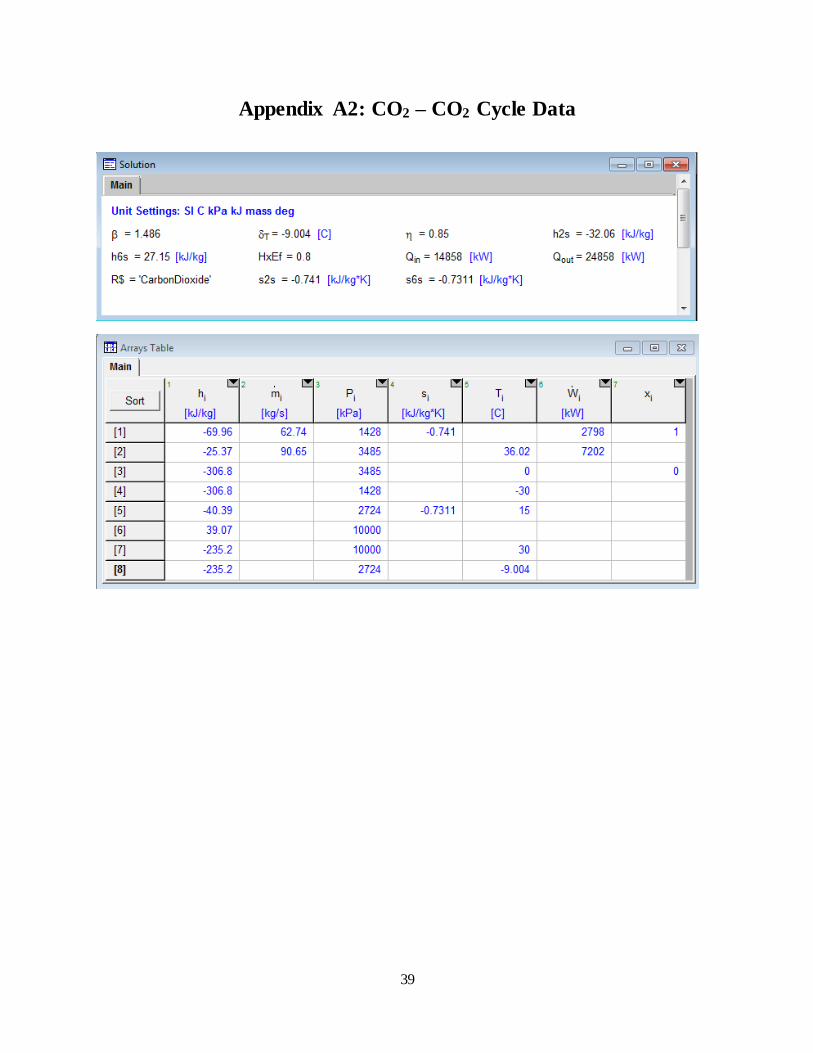
4.2. CO2 – CO2 System
Table 2: CO2 - CO2 system energy and performance results
Bottom Cycle Top Cycle Total
Work In (MW) 2.80 7.20 10.0
Flow Rate (kg/s) 62.74 90.65 -
Available Cooling (MW) 14.86 - 14.86
C.O.P. - - 1.49
The CO2-CO2 cycle was designed
within the constraints listed in the
Methodology section to produce the results
shown in Table 2. The state values can be
visualized better in the pressure-enthalpy
diagram, shown in Figure 11. The input energy
to the system was limited by the 10 MW work
constraint, and it was split up so that most of
the work was performed by the high
temperature cycle, with the low temperature
cycle requiring 2.80 MW and the high temperature cycle requiring 7.20 MW. Both cycles’
evaporation temperatures were determined by performing parametric studies with each
temperature serving as the independent variables, while total COP and mass flow rate of both
cycles were the dependent variables. The temperature for the CO2 entering the low temperature
evaporator was chosen to be -30℃, and the temperature of the CO2 exiting the high temperature
side of the cascading heat exchanger was 15℃, which maximized COP while keeping flow rate
for CO2 below 100 kg/s. See Appendix A1: Parametric Study Results for CO2 – CO2 System for
Figure 11: CO2 - CO2 state diagram on pressure vs. enthalpy chart
with the blue cycle representing the low temperature side and the
orange cycle representing the high temperature side

19
a visualization of the study. Finally, this cycle can provide a 14.86 MW cooling load to the
cooling water. For all state values of the cycle, see Appendix A2: CO2 – CO2 Cycle Data.
4.3. CO2 – NH3 System
Table 3: CO2 - NH3 system energy and performance results
CO2 Cycle NH3 Cycle Total
Work In (MW) 4.21 5.79 10.0
Flow Rate (kg/s) 94.39 24.17 -
Available Cooling (MW) 22.35 - 22.35
C.O.P. - - 2.24
The CO2-NH3 cycle was designed within the constraints listed in the Methodology
section to produce the results shown in Table 3. The pressure-enthalpy diagram of the state
values is shown in Figure 12.The input
energy to the system was limited by the
10 MW work constraint, and it was split
up relatively evenly between the cycles,
with the low temperature cycle requiring
4.21 MW and the high temperature cycle
requiring 5.79 MW. The CO2 cycle’s
temperature entering the evaporator and
the NH3 cycle’s pressure exiting the
compressor were determined by
performing parametric studies with both
parameters serving as the independent variables, while total COP and mass flow rate of both
Figure 12: CO2 – NH3 state diagram on pressure vs. enthalpy chart with the
blue cycle representing the low temperature side and the orange cycle
representing the high temperature side

20
cycles were the dependent variables. The chosen temperature for CO2 was -30℃ and the chosen
pressure for NH3 was 1,250 kPa. These maximized COP while keeping flow rate for CO2 below
100 kg/s. The results from the parametric study can be visualized in Appendix B1: Parametric
Study Results for CO2 – NH3 System. Finally, this cycle can provide an 22.35 MW cooling load
to the cooling water. For all state values of the cycle, see Appendix B2: CO2 – NH3 Cycle Data.
4.4. CO2 – LiBr-H2O System Table 4: CO2 - LiBr-H2O system energy and performance results
CO2 Cycle LiBr – H2O
Cycle Total
Work In (MW) 8.04 <0.001 8.04
Heat In (MW) 0 30.0 30.0
Max. Flow Rate (kg/s) 100.0 83.8 -
Available Cooling (MW) 20.96 - 20.96
C.O.P. - - 0.762
The CO2 – LiBr-H2O cycle was also designed within the constraints and assumptions
listed for the cycles, but the water in the absorption cycle was required to have a temperature in
the evaporator greater than 0℃. This cycle produced the results shown in Table 4. This system’s
input energy was limited not by work but by heat to the absorption cycle, which was capped at
30 MW. The compression cycle required 8.04 MW. A pressure-enthalpy diagram for this system
is less applicable, because the absorption cycle gains and releases energy mainly based on the
LiBr-H2O solution’s mass makeup, not its pressure and enthalpy. For this cycle, the evaporation
temperature of the absorption cycle was limited to 5℃, although it ended up being 7℃. The
generator temperature was set to be 90℃. The temperature of the CO2 entering the evaporator
and the temperature of the CO2 leaving the cascade heat exchanger were varied in a parametric

21
study like the ones performed in the first two cycles; the CO2 entering the evaporator was chosen
to be -40oC and the CO2 leaving the heat exchanger was set to 10℃. The results from the study
are illustrated in Appendix C1: Parametric Study Results from CO2 – LiBr-H2O System. The
available cooling from the system was determined to be 20.9 MW. For all state values of the
cycle, see Appendix C2: CO2 – LiBr-H2O Cycle Data.
4.5. CO2 – H2O-NH3 System Table 5: CO2 - H2O-NH3 system energy and performance results
CO2 Cycle H2O – NH3
Cycle Total
Work In (MW) 1.00 <0.001 1.00
Heat In (MW) 0.0 30.0 30.0
Max. Flow Rate (kg/s) 55.89 51.06 -
Available Cooling (MW) 13.91 - 13.91
C.O.P. - - 0.449
The CO2 – H2O-NH3 cycle was also designed within the constraints and assumptions
listed for the cycles, but the ammonia did not have the same constraint as the water in the
previous system, as its freezing point is -77.7℃. This cycle produced the results shown in Table
5. This system’s input energy was limited not by work but by heat to the absorption cycle, which
was capped at 30 MW. The compression cycle required only 1 MW of work. As noted for the
previous system, a pressure-enthalpy diagram is less applicable here. For the absorption cycle,
the temperature of the ammonia exiting the cascading heat exchanger was set to -12℃ and the
temperature of the carbon dioxide entering the low temperature evaporator was set to -20℃, but
the for this system, the temperature of the weak solution leaving the absorber and the amount of
work required for the compressor were varied in a parametric study. The dependent variable was
the cooling load available to act on the cooling water. The results from this study are shown in

22
Appendix D1: Parametric Study Results for CO2 – H2O-NH3. The available cooling from the
system was determined to be 13.9 MW. For all state values of the cycle, see Appendix D2: CO2
– H2O-NH3 Cycle Data.
4.6. Baseline Flow Rate After determining the cooling loads available from each cycle and cooling water
temperature requirements for each region, the baseline water use should be determined for each
situation. The baseline case is simply the amount of water needed to cool the hot working water
in the condenser. Based on EPRI standards, the hot working water comes in to the condenser as
steam at 50℃ and leaves as a saturated liquid, also at 50℃, with a flow rate of 315 kg/s. Based on
the enthalpies of the water at those two states, the required cooling was determined to be 750.6
MW. The equation for this is shown in Equation 1.
ṁℎ𝑜𝑡 × (ℎ𝑜𝑢𝑡 − ℎ𝑖𝑛) = 𝑄𝑐𝑜𝑛𝑑 = 315
𝑘𝑔
𝑠× (2592.1
𝑘𝐽
𝑘𝑔− 209.3
𝑘𝐽
𝑘𝑔) = 750.6 𝑀𝑊 (1)
The average cooling water and ambient air temperatures for each region, determined
from NCDC and USGS data as discussed in Section 3.4, were used to determine the properties of
the cooling water and various temperature constraints in the cooling systems. These temperatures
are shown in Table 6.
Table 6: Estimated average surface water and ambient air temperatures for each region
Northeast Midwest Southeast West
Water Temperature (℃) 12.8 19.5 24.0 15.8
Air Temperature (℃) 11.9 11.4 22.6 20.4
23
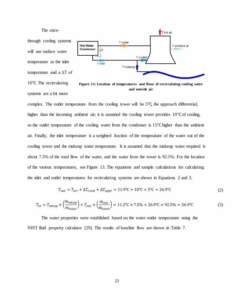
The once-
through cooling systems
will use surface water
temperature as the inlet
temperature and a ΔT of
10℃. The recirculating
systems are a bit more
complex. The outlet temperature from the cooling tower will be 5℃, the approach differential,
higher than the incoming ambient air; it is assumed the cooling tower provides 10℃ of cooling,
so the outlet temperature of the cooling water from the condenser is 15℃ higher than the ambient
air. Finally, the inlet temperature is a weighted fraction of the temperature of the water out of the
cooling tower and the makeup water temperature. It is assumed that the makeup water required is
about 7.5% of the total flow of the water, and the water from the tower is 92.5%. For the location
of the various temperatures, see Figure 13. The equations and sample calculations for calculating
the inlet and outlet temperatures for recirculating systems are shown in Equations 2 and 3.
𝑇𝑜𝑢𝑡 = 𝑇𝑎𝑖𝑟 + ∆𝑇𝑐𝑜𝑛𝑑 + ∆𝑇𝑎𝑝𝑝𝑟 = 11.9℃ + 10℃ + 5℃ = 26.9℃ (2)
𝑇𝑖𝑛 = 𝑇𝑚𝑘𝑢𝑝 × (
ṁ𝑚𝑘𝑢𝑝
ṁ𝑡𝑜𝑡𝑎𝑙
) + 𝑇𝑜𝑢𝑡 × (ṁ𝑜𝑢𝑡
ṁ𝑡𝑜𝑡𝑎𝑙
) = 11.2℃ × 7.5% + 26.9℃ × 92.5% = 26.9℃ (3)
The water properties were established based on the water outlet temperature using the
NIST fluid property calculator [29]. The results of baseline flow are shown in Table 7.
Figure 13: Location of temperatures and flows of recirculating cooling water
and outside air

24
Table 7: Baseline flow and parameter results based on region water and air properties and cooling type
Northeast Midwest Southeast West
Once-
through Recirculating
Once-
through Recirculating
Once-
through Recirculating
Once-
through Recirculating
Inlet Temp.
(℃) 11.2 16.5 17.3 16.5 24.0 27.3 15.8 24.7
Air Temp.
(℃) 11.9 11.4 22.6 20.4
Outlet Temp.
(℃) 21.2 26.9 27.3 26.4 34.0 37.6 25.8 35.4
Water
Density
(kg/m3)
997.98 996.59 996.48 996.70 994.40 993.13 996.86 993.92
Water
Specific Heat
(kJ/kg K)
4.183 4.181 4.180 4.181 4.182 4.179 4.181 4.179
ΔT (℃) 10.00 10.43 10.00 9.93 10.00 10.27 10.00 10.72
Baseline Flow
Rate (kg/s) 17,944 17,219 17,955 18,076 17,950 17,489 17,953 16,754
4.7. Water Savings
Now that the baseline flow has been established, the total water savings for each kind of
plant and refrigeration strategy can be determined. Regionally, the water savings will differ
slightly because the properties of water, like density and heat capacity, vary at different
temperatures. The water savings from the refrigeration cycles and using surface water as the inlet
or makeup water are shown in Table 8, Table 9, Table 10, and Table 11. The water flow rate
savings are calculated by using Equation 4, and sample calculations are shown; the makeup
water savings for recirculating systems are calculated using Equation 5, which was developed in
Perry’s Chemical Engineers Handbook [22].
ṁ𝑠𝑣𝑑 =
𝑄𝑟𝑒𝑓𝑟𝑔
∆𝑇 × 𝑐𝑝=
14.86 𝑀𝑊
10℃ × 4.1831𝑘𝐽𝑘𝑔
= 355.2𝑘𝑔
𝑠 (4)
ṁ𝑐𝑜𝑛𝑠_𝑠𝑣𝑑 = ((55.08) ×
ṁ𝑠𝑣𝑑
𝜌) × 1.25 + (7.2) ×
ṁ𝑠𝑣𝑑
𝜌 (5)

25
As mentioned in earlier sections, the relevant water savings for once-through systems are
the flow savings, which correspond to a reduction in water withdrawal, whereas the relevant
water savings for recirculating systems are the makeup water savings, which corresponds to
consumption savings.
Table 8: Flow savings with the addition of a CO2-CO2 refrigeration cycle for each region and cooling type
Northeast
Midwest
Southeast
West
Once-
through Recirculating
Once-
through Recirculating
Once-
through Recirculating
Once-
through Recirculating
Baseline Flow
Rate (kg/s) 17,953 17,228 17,965 18,086 17,960 17,498 17,963 16,763
Flow Rate with
Refrigeration
(kg/s)
17,598 16,887 17,609 17,728 17,604 17,152 17,607 16,432
Flow Savings
(kg/s) 355.2 340.9 355.5 357.9 355.4 346.2 355.4 331.7
Makeup Water
Savings (kg/s) - 7.23 - 7.58 - 7.36 - 7.05
Percent of Total
Saved 2.0%
Table 9: Flow savings with the addition of a CO2-NH3 refrigeration cycle for each region and cooling type
Northeast
Midwest
Southeast
West
Once-
through Recirculating
Once-
through Recirculating
Once-
through Recirculating
Once-
through Recirculating
Baseline Flow
Rate (kg/s) 17,953 17,228 17,965 18,086 17,960 17,498 17,963 16,763
Flow Rate with
Refrigeration
(kg/s)
17,419 16,715 17,430 17,548 17,425 16,977 17,428 16,265
Flow Savings
(kg/s) 534.3 512.7 534.6 538.2 534.5 520.7 534.6 498.9
Makeup Water
Savings (kg/s) - 10.9 - 11.4 - 11.1 - 10.6
Percent of Total
Saved 3.0%

26
Table 10: Flow savings with the addition of a CO2 - LiBr-H2O refrigeration cycle for each region and cooling
type
Northeast
Midwest
Southeast
West
Once-
through Recirculating
Once-
through Recirculating
Once-
through Recirculating
Once-
through Recirculating
Baseline Flow
Rate (kg/s) 17,953 17,228 17,965 18,086 17,960 17,498 17,963 16,763
Flow Rate with
Refrigeration
(kg/s)
17,452 16,747 17,463 17,581 17,458 17,010 17,461 16,296
Flow Savings
(kg/s) 501.1 480.8 501.4 504.8 501.2 488.4 501.3 467.9
Makeup Water
Savings (kg/s) - 10.2 - 10.7 - 10.4 - 9.9
Percent of Total
Saved 2.8%
Table 11: Flow savings with the addition of a CO2 – H2O-NH3 refrigeration cycle for each region and cooling
type
Northeast
Midwest
Southeast
West
Once-
through Recirculating
Once-
through Recirculating
Once-
through Recirculating
Once-
through Recirculating
Baseline Flow
Rate (kg/s) 17,953 17,228 17,965 18,086 17,960 17,498 17,963 16,763
Flow Rate with
Refrigeration
(kg/s)
17,621 16,909 17,632 17,751 17,627 17,174 17,630 16,453
Flow Savings
(kg/s) 332.5 319.1 332.7 335.0 332.6 324.1 332.7 310.5
Makeup Water
Savings (kg/s) - 6.8 - 7.1 - 6.9 - 6.6
Percent of Total
Saved 1.9%
4.8. Costs and Benefits of Refrigeration Cycle Recommendations
With the savings for all the refrigeration cycles and water sources determined, the final
step is to determine the most appropriate water reduction strategy for each region and cooling
type and determine the economic benefits and costs of the strategy. The annual economic

27
benefits of the cycle are determined by applying an estimate for the cost of water to power plants
developed by Ulrich, et al [23], although, as stated earlier, economic savings cannot be
appropriately calculated for recirculating systems that consume water as opposed to withdrawing
it. This equation is shown below in Equation 6.
𝑐𝑜𝑠𝑡𝑤𝑎𝑡𝑒𝑟 ,
$
𝑘𝑔𝑠
= [(0.0001 + 3 × 10⁻⁵ × (ṁ𝑐.𝑤.
𝜌)) × 𝐶𝑃𝐼 + 0.003 × 𝑐𝑜𝑠𝑡𝑓𝑢𝑒𝑙] × 𝜌 (6)
The annual energy costs of the cycles were determined by using the average price of
industrial electricity for regions designated by EIA that were the most like regions used in this
study. These prices can be seen in Table 12 [30].
Table 12: Estimated average price of industrial electricity based on region
Region Northeast Midwest Southeast West
Price of Electricity ($/kWh)
$0.0688 $0.0704 $0.0691 $0.0822
The annual energy costs were assumed to be the annual energy use of the compressors
multiplied by the price of electricity. The energy for heat in the absorption cycles was assumed
to cost nothing, as it could be captured as waste heat from a typical power plant. This is not
entirely true, as there would have to some energy put into making the heat usable, but compared
to the compression work, it is assumed to be negligible. The annual energy of each cycle is
shown in Table 13, and the annual energy cost will be determined for the cooling strategy used in
each region. The capital costs of the refrigeration cycles were assumed to be equal to the costs of
the compressors required by the systems because compressors would be by far the most
expensive part of a refrigeration cycle. The cost of the compressors was determined by a
compressor cost rating system developed by Amin Almasi [31]; the costs, outlined in Table 13,

28
are just estimates but can provide a good idea of the magnitude of savings necessary for the
system to be economically viable.
Table 13: Estimated annual energy use and capital cost of refrigeration cycles
CO2-CO2 CO2-NH3 CO2 - LiBr-H2O CO2 – H2O-NH3
Annual Energy Use (kWh/year)
87,600,000 87,600,000 64,272,120 8,760,000
Capital Cost ($) $14,650,000 $14,380,000 $9,692,778 $2,152,778
For the Northeast region, the refrigeration cycle recommended was the CO2 – H2O-NH3
cycle, because the region does not experience a lot of water stress, so it does not make sense to
spend a lot of money, annually and upfront, to reduce cooling water use. For the Midwest region,
the refrigeration cycle recommended was the CO2 – LiBr-H2O cycle, because the region does
experience some water stress along its major rivers like the Ohio and Mississippi. For the
Southeast region, the refrigeration cycle recommended was also the CO2 – LiBr-H2O cycle,
because the region experiences some water stress along the Mississippi, but, more importantly,
the region struggles with cooling water return temperature for the once-through systems, so in
exchange for some water reduction, the return temperature could be reduced using the
refrigeration cycle. Still, it is not paramount for the cycle to have the maximum reduction of
water use in exchange for high costs, so the CO2 – NH3 cycle, which has the highest water
reduction potential, was not recommended. For the West region, the refrigeration cycle
recommended was the CO2 – NH3 cycle, because the region experiences extreme water stress in
many different areas that have power plants. There are power plants that this may not apply to in
the West region, but in the West more than any region, maximum water savings are paramount.
The water savings, cost savings, and energy costs for each recommendation are shown in Table
14. The equations used to calculate water saved and energy cost, along with sample calculations,
are shown in Equations 7 and 8.
29
𝑊𝑎𝑡𝑒𝑟 𝑆𝑎𝑣𝑒𝑑𝑎𝑛𝑛𝑢𝑎𝑙 =
ṁ𝑠𝑣𝑑
𝜌× 3,600
𝑠
ℎ𝑟× 8,760
ℎ𝑟
𝑦𝑟× 264.17
𝑔𝑎𝑙
𝑚3 = 2.78 × 10⁹𝑔𝑎𝑙
𝑦𝑒𝑎𝑟 (7)
𝐸𝑛𝑒𝑟𝑔𝑦 𝐶𝑜𝑠𝑡𝑎𝑛𝑛𝑢𝑎𝑙 = 𝑊𝑖𝑛 × 8,760
ℎ𝑟
𝑦𝑒𝑎𝑟× 𝐶𝑜𝑠𝑡𝑒𝑙𝑒𝑐 = 10,000 𝑘𝑊 × 8,760
ℎ𝑟
𝑦𝑒𝑎𝑟×
$0.0688
𝑘𝑊
=$6,026,880
𝑦𝑒𝑎𝑟
(8)
Table 14: Water savings and economics costs & benefits for cooling strategy recommendations
Region Northeast Midwest Southeast West
Recommended
Cycle CO2-H2O-NH3 CO2-LiBr-H2O CO2-LiBr-H2O CO2-NH3
Cooling Type Once-
through Recirculating
Once-
through Recirculating
Once-
through Recirculating
Once-
through Recirculating
Water Saved
(Million gal/year) 2,776 56.5 4,192 89.4 4,199 87.1 4,467 88.9
Annual Water
Cost Savings
($/year)
$787,394 $16,047 $1,188,990 $25,363 $1,191,108 $24,724 $1,267,213 $25,231
Annual Energy
Cost ($/year) $602,688 $4,524,757 $4,441,203 $7,200,720
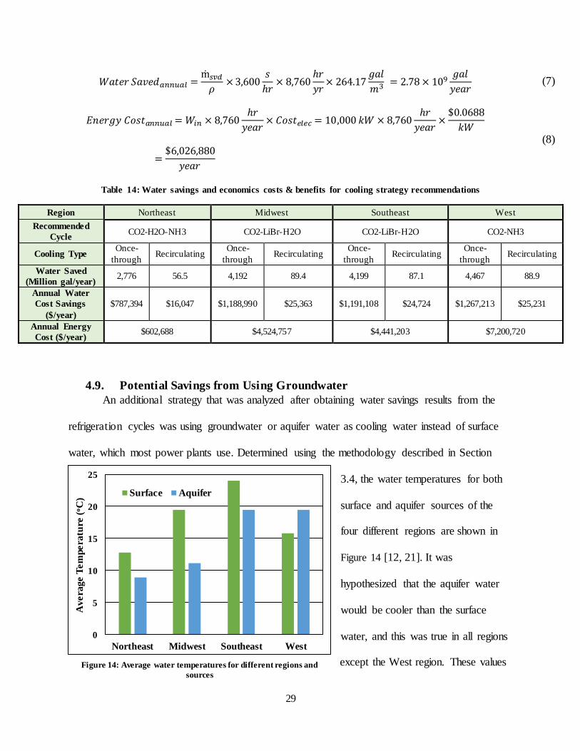
4.9. Potential Savings from Using Groundwater
An additional strategy that was analyzed after obtaining water savings results from the
refrigeration cycles was using groundwater or aquifer water as cooling water instead of surface
water, which most power plants use. Determined using the methodology described in Section
3.4, the water temperatures for both
surface and aquifer sources of the
four different regions are shown in
Figure 14 [12, 21]. It was
hypothesized that the aquifer water
would be cooler than the surface
water, and this was true in all regions
except the West region. These values
0
5
10
15
20
25
Northeast Midwest Southeast West
Ave
rage
Tem
pera
ture
(oC
)
Surface Aquifer
Figure 14: Average water temperatures for different regions and
sources

30
should be used cautiously, as temperatures vary widely from source to source, and the regions
used each cover many different climate zones. However, they should serve as a good comparison
tool.
The savings that are associated with using groundwater, especially for the once-through
systems, should be treated as rough theoretical estimates, as using ground water in these
quantities may not be possible, or it may deplete desperately needed drinking water sources in
some areas. In fact, the amount of water that would be required for once-through systems is most
likely an unreasonable strain on groundwater sources that are used for other purposes. For this
reason, the percent savings for once-through systems are not shown, so as not to present
potentially misleading results. The results for flow and makeup water savings are shown in Table
15.

31
Table 15: Water flow savings created from using groundwater instead of surface water for cooling
Northeast Midwest Southeast West
Once-
through Recirculating
Once-
through Recirculating
Once-
through Recirculating
Once-
through Recirculating
Inlet Temp.
(℃) 8.9 16.3 11.1 16.0 19.4 27.0 19.4 25.0
Air Temp. (℃) 11.9 11.4 22.6 20.4
Outlet Temp.
(℃) 21.2 26.9 27.3 26.4 34.0 37.6 25.8 35.4
Water Density
(kg/m3) 997.98 996.59 996.48 996.7 994.4 993.13 996.86 993.9
Water Specific
Heat
(kJ/kg K)
4.183 4.181 4.180 4.181 4.182 4.179 4.181 4.17
ΔT (℃) 12.30 10.60 16.20 10.40 14.60 10.62 6.40 10.4
Baseline Flow
Rate (kg/s) 17,944 17,219 17,955 18,076 17,950 17,489 17,953 16,75
Flow Rate
Using
Groundwater
(kg/s)
14,588 16,938 11,083 17,268 12,295 16,920 28,052 17,18
Flow Savings
(kg/s) 3,355 280 6,872 808 5,656 568 -10,099 -43
Makeup
Water Savings
(kg/s) - 5.9 - 17.1 - 12.1 - -9.2
Percent of
Total Saved - 1.6% - 4.5% - 3.3% - -2.6%
5. Summary and Conclusions The goal of this study was to design and evaluate strategies for reducing cooling water
use in power plants. For recirculating plants, this meant reducing water consumption, and for
once-through plants, this meant reducing water withdrawal. To evaluate the effectiveness of the
strategies that were developed, four regions were established and water and air temperatures
were estimated for the regions. To reduce the cooling water use, the temperature differential
across the hot water condenser needed to be increased. To allow for this without increasing the
outlet temperature, it was necessary to design refrigeration cycles to reduce the temperature of

32
cooling water after the hot water condenser. Cycles were designed in accordance with
assumptions and constraints that were developed based on typical power plant properties,
refrigerant qualities, and water and air temperatures, among other things. After the cycles were
designed and water temperatures established, the flow reduction, and thus water savings, could
be established. A strategy for each region and cooling type was suggested based on the water
savings and the different water landscapes in the various regions. To provide an idea of how
economically feasible the strategies were, the water saving cost benefits, energy costs, and cycle
capital costs were all estimated. For the sake of investigating strategies that could be coupled
with the refrigeration cycles, different water sources were also evaluated to determine if drawing
water from those sources could help reduce cooling water use based on the temperature of the
other sources.
The most important metric gained from this research is the potential amount of water that
could be saved. The energy-water nexus has become one of the largest issue surrounding power
plants in recent years, and there has been a call for solutions to help reduce the water use in
power plants. There will not be one simple solution that solves the problem; it will be solved
iteratively, with unique solutions implemented at different power plants. That is why the
economic results of this research helpful for comparison, but are not the best way to judge
feasibility or significance. There is neither a high confidence in their accuracy or precision, nor
does the economic cost and benefit capture all of the factors involved in how the reduction of
cooling water will affect the power plant and its surrounding region. With that said, a single
once-through plant could see water cost savings of around $1,000,000 per year, which is perhaps
marginal compared to the power plant profits, but cannot be ignored in terms of magnitude. For
recirculating plants, the savings are smaller at around $25,000 per year, but this does not capture

33
the benefits of keeping water in the local watershed that would otherwise have been lost to
evaporation or another form of consumption. Also, as populations and economies continue to
grow, the price of water will continue to rise due to increased scarcity, along with increased
demand for agriculture and energy production. So, while these strategies may not be
economically beneficial in current economic times, it is easy to see how water will start to
become the U.S.’s most valuable and expensive resources, especially in certain regions like
California.
In terms of specific results, the water savings for these cycles is significant. Regardless of
the region or plant type, using these refrigeration cycles could result in saving two to three
percent of all water used. While this may not sound like a huge reduction, this corresponds to
around 4 billion gallons of water per year saved from withdrawal at a single once-through plant
and 80 million gallons of water per year saved from consumption at a single recirculating plant.
This is a huge amount of water that would be newly available to the surrounding areas for
drinking water, industrial use, or ecological processes. Specifically, the ability to save tens of
millions of gallons of water from consumption at a single recirculating plant is extremely
significant for areas that experience a lot of water stress, like the Southwest, the Mississippi
River region, and the eastern part of Pacific Coast states. Currently, economic metrics do not
appropriately capture the true value of water in these regions, but the value of water will
continue to rise in coming years, as the rate of water use continues to increase, while water
availability remains the same or decreases. There is even potential for power plants to trade their
water savings, as some industries trade electricity savings, although the infrastructure for this
kind of system would require more research.

34
The water savings for once-through systems is also important, although for different
reasons. In many water ecosystems, the rising temperature of the water has decreased the oxygen
availability in the water and has ripened environments for harmful algal blooms, as mentioned in
the introduction. If the thermal mass added to these rivers from high-temperature cooling water
can be decreased, either by a reduction in flow or a reduction in temperature, which are both
possible through the refrigeration cycles, these environmentally and ecologically harmful events
can be slowed, if not eliminated.
It is also important to note that most of the systems chosen use heat as an input for the
absorption cycle. This was treated as “free” energy in this study due to the ability to capture a
certain amount of usable waste heat from the power plant, but there is significant infrastructure
that must be implemented to capture this heat, and it may not be available for all power plants.
This reasoning goes for the use of aquifer water as well. The savings results for using
groundwater instead of surface water at recirculating plants, although not at once-through plants
due to the unreasonable stress they would put on an aquifer, are just as significant as, if not more
than, the potential savings from the refrigeration cycles. In the Midwest and Southeast, savings
could be as high as 4% of total cooling water consumption. However, there are concerns with the
impact of extracting large amounts of ground water from an aquifer, and along with that also
comes economic and logistical issues about the infrastructure that would need to be
implemented. Nonetheless, neither of these issues are new to the water or energy industry, and
existing solutions can most likely be adapted to fit the cases presented in this research. Future
research into the effects of using significant amounts of groundwater, on the order of billions of
gallons per year, for power plant cooling could reveal another strategy for reducing the amount
cooling water use at power plants.

35
The impact of this research is evident in the water savings that are shown to be possible,
but there are many steps that must be taken before these strategies can be put in place. Now that
the cycles have been theoretically designed, the ones that were selected for use in different
regions need to be designed at a lab scale to assure that they provide the expected cooling based
on the scaled-down size they were designed at. Next, specific power plants should be chosen as
case studies to determine logistically the best way to lay out these refrigeration systems and,
where applicable, the groundwater extraction. This includes how to harness waste heat and how
to source energy for the compressors. The groundwater extraction would also likely require
environmental surveys and governmental permission. Ultimately, for this research to be used as
motivation for power plants to install these refrigeration cycles, the true value of water for
different regions will have to be quantified or at least understood well enough to weight the costs
and benefits of these strategies.
36
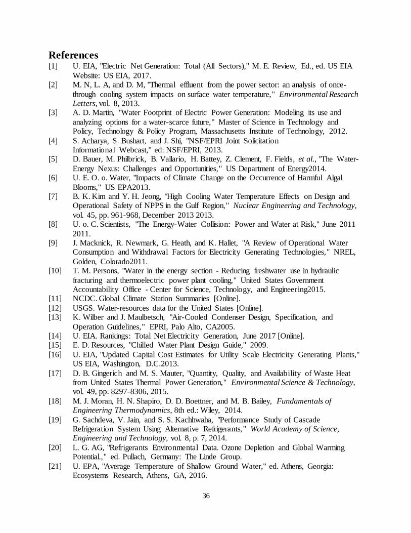
References [1] U. EIA, "Electric Net Generation: Total (All Sectors)," M. E. Review, Ed., ed. US EIA
Website: US EIA, 2017. [2] M. N, L. A, and D. M, "Thermal effluent from the power sector: an analysis of once-
through cooling system impacts on surface water temperature," Environmental Research Letters, vol. 8, 2013.
[3] A. D. Martin, "Water Footprint of Electric Power Generation: Modeling its use and
analyzing options for a water-scarce future," Master of Science in Technology and Policy, Technology & Policy Program, Massachusetts Institute of Technology, 2012.
[4] S. Acharya, S. Bushart, and J. Shi, "NSF/EPRI Joint Solicitation Informational Webcast," ed: NSF/EPRI, 2013.
[5] D. Bauer, M. Philbrick, B. Vallario, H. Battey, Z. Clement, F. Fields, et al., "The Water-
Energy Nexus: Challenges and Opportunities," US Department of Energy2014. [6] U. E. O. o. Water, "Impacts of Climate Change on the Occurrence of Harmful Algal
Blooms," US EPA2013. [7] B. K. Kim and Y. H. Jeong, "High Cooling Water Temperature Effects on Design and
Operational Safety of NPPS in the Gulf Region," Nuclear Engineering and Technology,
vol. 45, pp. 961-968, December 2013 2013. [8] U. o. C. Scientists, "The Energy-Water Collision: Power and Water at Risk," June 2011
2011. [9] J. Macknick, R. Newmark, G. Heath, and K. Hallet, "A Review of Operational Water
Consumption and Withdrawal Factors for Electricity Generating Technologies," NREL,
Golden, Colorado2011. [10] T. M. Persons, "Water in the energy section - Reducing freshwater use in hydraulic
fracturing and thermoelectric power plant cooling," United States Government Accountability Office - Center for Science, Technology, and Engineering2015.
[11] NCDC. Global Climate Station Summaries [Online].
[12] USGS. Water-resources data for the United States [Online]. [13] K. Wilber and J. Maulbetsch, "Air-Cooled Condenser Design, Specification, and
Operation Guidelines," EPRI, Palo Alto, CA2005. [14] U. EIA. Rankings: Total Net Electricity Generation, June 2017 [Online]. [15] E. D. Resources, "Chilled Water Plant Design Guide," 2009.
[16] U. EIA, "Updated Capital Cost Estimates for Utility Scale Electricity Generating Plants," US EIA, Washington, D.C.2013.
[17] D. B. Gingerich and M. S. Mauter, "Quantity, Quality, and Availability of Waste Heat from United States Thermal Power Generation," Environmental Science & Technology, vol. 49, pp. 8297-8306, 2015.
[18] M. J. Moran, H. N. Shapiro, D. D. Boettner, and M. B. Bailey, Fundamentals of Engineering Thermodynamics, 8th ed.: Wiley, 2014.
[19] G. Sachdeva, V. Jain, and S. S. Kachhwaha, "Performance Study of Cascade Refrigeration System Using Alternative Refrigerants," World Academy of Science, Engineering and Technology, vol. 8, p. 7, 2014.
[20] L. G. AG, "Refrigerants Environmental Data. Ozone Depletion and Global Warming Potential.," ed. Pullach, Germany: The Linde Group.
[21] U. EPA, "Average Temperature of Shallow Ground Water," ed. Athens, Georgia: Ecosystems Research, Athens, GA, 2016.

37
[22] Various, Perry's Chemical Engineer's Handbook: McGraw-Hill, 1997. [23] G. D. Ulrich and P. T. Vasudevan. (2006, How To Estimate Utility Costs.
[24] A. Cavallini and C. Zilio, "Properties of CO2 as a Refrigerant," International Journal of Low-Carbon Technologies, pp. 225-249, 2007.
[25] NIST. Ammonia [Online]. [26] B. Babu and G. M. P. Yadav, "Performance Analysis of Lithium-Bromide Water
Absorption Refrigeration System Using Waste Heat of
Boiler Flue Gases," International Journal of Engineering Research and Management, vol. 2, pp. 2349-2058, 2015.
[27] I. Horuz, "A Comparison Between Ammonia-Water and Water-Lithium Bromide Solutions in Vapor Absorption Refrigeration Systems," International Communications in Heat Mass Transfer, vol. 25, pp. 711-721, 1998.
[28] M. Y. Taib, A. A. Aziz, and A. B. S. Alias, "Performance Analysis of a Domestic Refrigerator," presented at the National Conference in Mechanical Engineering Research
and Postgraduate Students, Pahang, Malaysia, 2010. [29] NIST. Isobaric Properties for Water [Online]. [30] U. EIA. Average Price of Electricity to Ultimate Customers by End-Use Sector [Online].
[31] A. Almasi. (2014, How Much Will Your Compressor Installation Cost?

38
Appendix A1: Parametric Study Results for CO2 – CO2 System
39
Appendix A2: CO2 – CO2 Cycle Data

40
Appendix A3: CO2 – CO2 Cycle EES Code "Refrigerant"
R$='CarbonDioxide'
"Assumptions"
W_dot[2]+W_dot[1]=10000 [kW]
eta=0.85 "Efficiency of compressors"
HxEf=0.8
"State 7"
P[7]=10000[kPa]
T[7]=30[C]
h[7]=enthalpy(R$,T=T[7],P=P[7])
"State 8"
h[8]=h[7]
{T[8]=-2.5}
P[8]=pressure(R$,h=h[8],T=T[8])
"State 5"
P[5]=P[8]
T[5]=15[C]
h[5]=enthalpy(R$,P=P[5],T=T[5])
s[5]=entropy(R$,P=P[5],T=T[5])
"State 6s"
s6s=s[5]
P[6]=P[7]
h6s=enthalpy(R$,s=s6s,P=P[6])
"State 6"
h[6]=(h6s-h[5])/eta+h[5]
"Heat Exchanger"
HxEf=(T[2]-T[3])/(T[2]-T[8])
"State 4"
T[4]=-30[C]
h[4]=h[3]
P[4]=pressure(R$,h=h[4],T=T[4])
"State 1"
P[1]=P[4]
x[1]=1
h[1]=enthalpy(R$,P=P[1],x=x[1])
s[1]=entropy(R$,P=P[1],x=x[1])
"State 2s"
s2s=s[1]
P[2]=P[3]
h2s=enthalpy(R$,s=s2s,P=P[2])

41
"State 2"
h[2]=(h2s-h[1])/eta+h[1]
T[2]=temperature(R$,h=h[2],P=P[2])
"State 3"
T[3]=0[C]
x[3]=0
P[3]=pressure(R$,x=x[3],T=T[3])
h[3]=enthalpy(R$,x=x[3],T=T[3])
"Equations"
m_dot[2]=W_dot[2]/(h[6]-h[5])
m_dot[1]=W_dot[1]/(h[2]-h[1])
(h[8]-h[5])*m_dot[2]=(h[3]-h[2])*m_dot[1]
Q_out=(h[6]-h[7])*m_dot[2]
Q_in=(h[1]-h[4])*m_dot[1]
beta=Q_in/(W_dot[1]+W_dot[2])
delta_T=T[8]-T[3]

42
Appendix B1: Parametric Study Results for CO2 – NH3 System
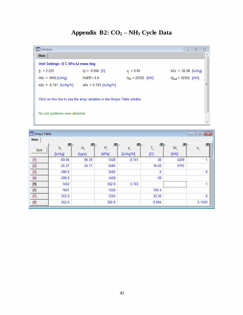
43
Appendix B2: CO2 – NH3 Cycle Data

44
Appendix B3: CO2 – NH3 Cycle Code "Assumptions"
W_dot[2]+W_dot[1]=10000 [kW]
eta=0.85 "Efficiency of compressors"
HxEff=0.8
"State 7"
P[7]=1250[kPa]
x[7]=0
h[7]=enthalpy('Ammonia',x=x[7],P=P[7])
T[7]=temperature('Ammonia',x=x[7],P=P[7])
"State 8"
h[8]=h[7]
P[8]=pressure('Ammonia',h=h[8],T=T[8])
x[8]=quality('Ammonia',h=h[8],T=T[8])
"State 5"
P[5]=P[8]
x[5]=1
h[5]=enthalpy('Ammonia',P=P[5],x=x[5])
s[5]=entropy('Ammonia',P=P[5],x=x[5])
"State 6s"
s6s=s[5]
P[6]=P[7]
h6s=enthalpy('Ammonia',s=s6s,P=P[6])
"State 6"
h[6]=(h6s-h[5])/eta+h[5]
T[6]=temperature('Ammonia',P=P[6],h=h[6])
"Heat Exchanger"
HxEff=(T[2]-T[3])/(T[2]-T[8])
"State 4"
T[4]=-30[C]
h[4]=h[3]
P[4]=pressure('CarbonDioxide' ,h=h[4],T=T[4])
"State 1"
P[1]=P[4]
x[1]=1
h[1]=enthalpy('CarbonDioxide' ,P=P[1],x=x[1])
s[1]=entropy('CarbonDioxide' ,P=P[1],x=x[1])
T[1]=temperature('CarbonDioxide' ,P=P[1],x=x[1])
"State 2s"
s2s=s[1]
P[2]=P[3]
h2s=enthalpy('CarbonDioxide' ,s=s2s,P=P[2])

45
"State 2"
h[2]=(h2s-h[1])/eta+h[1]
T[2]=temperature('CarbonDioxide',P=P[2],h=h[2])
"State 3"
T[3]=0[C]
x[3]=0
P[3]=pressure('CarbonDioxide' ,x=x[3],T=T[3])
h[3]=enthalpy('CarbonDioxide' ,x=x[3],T=T[3])
"Equations"
m_dot[2]=W_dot[2]/(h[6]-h[5])
m_dot[1]=W_dot[1]/(h[2]-h[1])
(h[8]-h[5])*m_dot[2]=(h[3]-h[2])*m_dot[1]
Q_out=(h[6]-h[7])*m_dot[2]
Q_in=(h[1]-h[4])*m_dot[1]
beta=Q_in/(W_dot[1]+W_dot[2])
delta_T=T[8]-T[3]

46
Appendix C1: Parametric Study Results from CO2 – LiBr-H2O
System

47
Appendix C2: CO2 – LiBr-H2O Cycle Data

48
Appendix C3: CO2 – LiBr-H2O Cycle Code
SI=2
{Input data}
Eff_Hx=0.8
Qg=30000
Phigh=7.445
T[4]=90
T[1]=40
Q[8]=0
Q[10]=1.0
x[4]=X_LIBR(T[4],Phigh,SI)
X[1]=X_LIBR(T[1],Plow,SI)
T[7]=T_LIBR(Phigh,x[3],SI)
{Set pressures}
Phigh=pressure(WATER,T=T[8],x=Q[8])
Plow=pressure(WATER,T=T[10],x=Q[10])
{Heat Exchanger}
Eff_Hx=(T[4]-T[5])/(T[4]-T[2])
{Heat transfer}
{Energy balance}
{Generator}
m[3]=m[4]+m[7]
{Overall mass balance}
m[3]*x[3]=m[4]*x[4]
{LiBr balance}
h[3]*m[3]-h[4]*m[4]-h[7]*m[7]+Qg=0 {Energy balance}
{Condenser}
Qc=m[7]*(h[7]-h[8])
{Energy balance}
{Refrigerant Valve}
h[9]=h[8]
{Energy balance}
{Evaporator}
Qe=m[9]*(h[10]-h[9]) {Energy
balance}
{Absorber}
m[10]*h[10]+h[6]*m[6]-Qa-m[1]*h[1]=0 {Energy balance}
{Solution expansion valve model}
h[6]=h[5]
{Energy balance}

49
{Pump calculation}
h[2]=h[1] {Energy balance}
{Trivial mass balances}
m[2]=m[1]
m[3]=m[2]
m[5]=m[4]
m[6]=m[5]
m[8]=m[7]
m[9]=m[8]
m[10]=m[9]
x[2]=X[1]
x[3]=x[2]
x[5]=x[4]
x[6]=x[5]
x[7]=0
x[8]=x[7]
x[9]=x[8]
x[10]=x[9]
{Compute thermodynamic properties}
h[1]=H_LIBR(T[1],X[1],SI)
h[2]=H_LIBR(T[2],x[2],SI)
h[3]=H_LIBR(T[3],x[3],SI)
h[4]=H_LIBR(T[4],x[4],SI)
h[5]=H_LIBR(T[5],x[5],SI)
CALL Q_LIBR(h[6],Plow,x[6],SI:q6b,T6b,Xl6b,hl6b,hv6b)
T[6]=T6b
h[7]=enthalpy(WATER,T=T[7],P=Phigh)
h[8]=enthalpy(WATER,T=T[8],x=0)
T[9]=temperature(WATER,h=h[9],P=Plow)
h[10]=enthalpy(WATER,T=T[10],x=1)
v1=V_LIBR(T[1],X[1],SI)
{Compute COP}
COP=Qe/(Win+Qg)
{Solution Circulation Ratio}
F=x[4]/(x[4]-x[3])
{Vapor quality at 9}
q[9]=quality(STEAM_NBS,h=h[9],P=Plow)
{Set Pressures}
P[1]=Plow
P[2]=Phigh
P[3]=Phigh
P[4]=Phigh
P[5]=Phigh

50
P[6]=Plow
P[7]=Phigh
P[8]=Phigh
P[9]=Plow
P[10]=Plow
{Set Vapor Quality}
Q[1]=0
Q[4]=0
Q[6]=Q6b*0.01 {Fraction}
{Q[9]=quality(STEAM_NBS,h=h[9],P=Plow)}
"CO2 Cycle"
"Refrigerant"
R$='CarbonDioxide'
"State 14"
T[14]=-40[C]
h[14]=h[13]
P[14]=pressure(R$,h=h[14],T=T[14])
s[14]=entropy(R$,h=h[14],T=T[14])
"State 11"
P[11]=P[14]
Q[11]=1
h[11]=enthalpy(R$,P=P[11],x=Q[11])
s[11]=entropy(R$,P=P[11],x=Q[11])
T[11]=temperature(R$,P=P[11],h=h[11])
"State 12s"
s12s=s[11]
P[12]=P[13]
h12s=enthalpy(R$,s=s12s,P=P[12])
"State 12"
h[12]=(h12s-h[11])/eta+h[11]
T[12]=temperature(R$,P=P[12],h=h[12])
s[12]=entropy(R$,P=P[12],h=h[12])
"State 13"
Eff_Hx=(T[12]-T[13])/(T[12]-T[9])
T[13]=10[C]
Q[13]=0
P[13]=pressure(R$,x=Q[13],T=T[13])
h[13]=enthalpy(R$,x=Q[13],T=T[13])
s[13]=entropy(R$,P=P[13],h=h[13])
"Equations"
m[11]=100
eta=0.85 "Efficiency of compressor"
m[11]=Win/(h[12]-h[11])
(h[10]-h[9])*m[10]=(h[12]-h[13])*m[11]
Qin=(h[14]-h[11])*m[11]
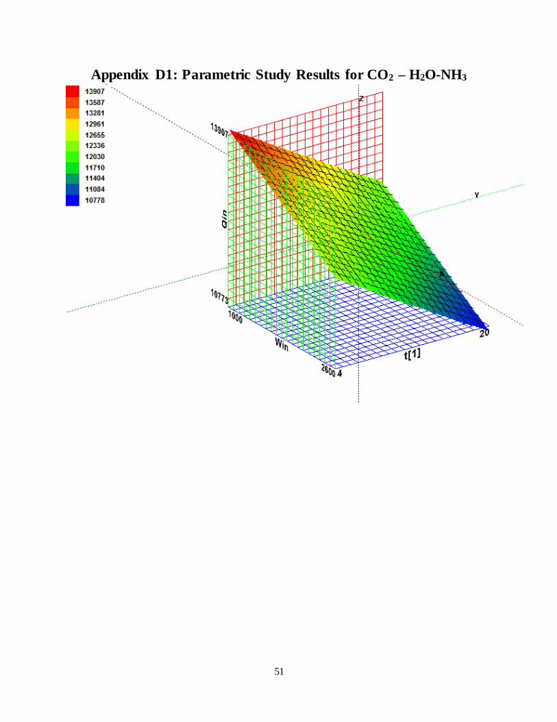
51
Appendix D1: Parametric Study Results for CO2 – H2O-NH3

52
Appendix D2: CO2 – H2O-NH3 Cycle Data

53
Appendix D3: CO2 – H2O-NH3 Cycle Data
THIS PROGRAM CALCULATES THE PERFORMANCE OF A SINGLE-STAGE
ABSORPTION SYSTEM WITH CONDENSATE PRECOOLING
"The following procedures are used to convert units"
PROCEDURE TPQ(TC,P,Q:x,h,v,s)
"given T (temperature), P (pressure) and Q (quality) in SI units,
this procedures returns x, h, v and s in SI units"
TK=TC+273.15
Pbar=P*.01
CALL NH3H2O(128,TK,Pbar,Q:TK,Pbar,x,h,s,u,v,Q)
END
PROCEDURE TPX(TC,P,x:Q,h,v,s)
"given T (temperature), P (pressure) and x (ammonia wt fraction) in SI
units, this procedure returns Q, h, v and s in SI units"
TK=TC+273.15
Pbar=P*.01
CALL NH3H2O(123,TK,Pbar,x:TK,Pbar,x,h,s,u,v,Q)
END
PROCEDURE PXQ(P,x,Q:TC,h,v,s)
"given P (pressure in bar), x (ammonia wt fraction) and Q, this procedure
returns T, h, v and s in SI units"
Pbar=P*.01
CALL NH3H2O(238,Pbar,x,Q:TK,Pbar,x,h,s,u,v,Q)
TC=TK-273.15
END
PROCEDURE PHX(P,h,x:TC,Q,v,s)
"given P (pressure in bar), enthalpy (J/g), and x (ammonia wt
fraction), this procedure returns T, Q, v and s in SI units"
Pbar=P*.01
CALL NH3H2O(234,Pbar,x,h:TK,Pbar,x,h,s,u,v,Q)
TC=TK-273.15
END
PROCEDURE TXQ(TC,x,Q:P,h,v,s)
"given T (temperature in C), Q (quality) and x (ammonia wt fraction) in SI
units, this procedure returns P, h, v and s in SI units"
TK=TC+273.15
CALL NH3H2O(138,TK,x,Q:TK,Pbar,x,h,s,u,v,Q)
P=Pbar*100
END
PROCEDURE PXS(P,x,s:TC,h,v,Q)
"given P (pressure in bar), x (ammonia wt fraction) and entropy s, this
procedure
returns T, h, v and Q in SI units"
Pbar=P*.01
CALL NH3H2O(235,Pbar,x,s:TK,Pbar,x,h,s,u,v,Q)
TC=TK-273.15
END
"This procedure calculates the amount of heat that is exchanged

54
in the solution heat exchanger"
PROCEDURE SHX(eshx,mls,mrs,ha,hb,hc,hd:hcc,hdd,qshx)
qls=mls*(hd-ha) "amount of heat on 'left side', rich solution"
qrs=mrs*(hb-hc) "amount of heat on 'right side', poor solution"
qmin=MIN(qls,qrs)
qshx=eshx*qmin "eshx is the sol. hx. effectiveness"
hcc=hb-eshx*qmin/mrs "calculation of outlet enthalpies"
hdd=ha+eshx*qmin/mls
END
"INPUT PARAMETERS"
"efficiencies"
eshx=0.8 "solution heat exchanger efectiveness"
f=(x[9]-x[4])/(x[3]-x[4]) "solution circulation ratio"
"temperatures"
t[12]=-12 " for state point, see diagram window"
t[10]=30
t[1]=5
tglide=T[12]-T[11]
"mass fractions"
x[9]=0.9996
x[1]-x[4]=Dx
Dx=0.20
"heat"
Qgen=30000 [kW]
"Pump Work"
Wp=0 [kW]
"Quality"
Q[12]=1
Q[10]=0.00
Q[7]=1
Q[9]=1
Q[1]=0
Q[4]=0
"governing equations"
"ABSORBER"
m[12]+m[6]=m[1]
m[12]*x[12]+m[6]*x[6]=m[1]*x[1]
m[12]*h[12]+m[6]*h[6]=m[1]*h[1]+Qabs
"DESORBER"
balm=m[8]+m[3]-(m[7]+m[4])
bala=m[8]*x[8]+m[3]*x[3]-(m[7]*x[7]+m[4]*x[4])
m[3]*h[3]+m[8]*h[8]+Qgen=m[7]*h[7]+m[4]*h[4]
CALL pxq(P[3],x[3],0:T3f,h3f,v3f,s3f)
T[7]=T3f
"RECTIFIER"
m[7]=m[9]+m[8]
m[7]*x[7]=m[9]*x[9]+m[8]*x[8]
m[7]*h[7]=m[9]*h[9]+m[8]*h[8]+Qrect
h[8]=h3f
x[8]=x[3]
"PUMP"

55
h[2]=h[1]
"EXPANSION VALVE"
h[5]=h[6]
"SHX"
CALL tpx(T[2],P[5],x[5]:Q5e,h5e,v5e,s5e)
CALL tpx(T[4],P[3],x[3]:Q3e,h3e,v3e,s3e)
CALL shx(eshx,m[2],m[4],h[2],h[4],h5e,h3e:h[5],h[3],Qshx)
"CONDENSER"
Qcond=m[9]*(h[9]-h[10])
"EVAPORATOR"
Qevap=m[12]*(h[12]-h[11])
"EXPANSION VALVE"
h[10]=h[11]
"OVERALL"
COP=Qin/(Wp+Win+Qgen)
checkQ=Qgen+Qevap+Wp-(Qrect+Qcond+Qabs)
pratio=phigh/plow
"SET PRESSURES"
p[1]=plow
p[2]=phigh
P[3]=phigh
p[4]=phigh
P[5]=phigh
P[6]=plow
p[7]=phigh
p[8]=phigh
p[9]=phigh
p[10]=phigh
p[11]=plow
p[12]=plow
"TRIVIAL MASS BALANCES"
m[1]=m[2]
m[2]=m[3]
m[4]=m[5]
m[5]=m[6]
m[9]=m[10]
m[10]=m[11]
m[11]=m[12]
"TRIVIAL NH3 BALANCES"
x[1]=x[2]
x[2]=x[3]
x[4]=x[5]
x[5]=x[6]
x[9]=x[10]
x[10]=x[11]
x[11]=x[12]
"STATE POINTS"
CALL txq(t[1],x[1],Q[1]:p[1],h[1],v[1],s[1])
CALL phx(p[2],h[2],x[2]:T[2],Q[2],v[2],s[2])
CALL phx(P[3],h[3],x[3]:T[3],Q[3],v[3],s[3])
CALL pxq(p[4],x[4],Q[4]:T[4],h[4],v[4],s[4])

56
CALL phx(P[5],h[5],x[5]:T[5],Q[5],v[5],s[5])
CALL phx(P[6],h[6],x[6]:T[6],Q[6],v[6],s[6])
CALL tpq(T[7],p[7],Q[7]:x[7],h[7],v[7],s[7])
CALL phx(p[8],h[8],x[8]:T[8],Q[8],v[8],s[8])
CALL pxq(p[9],x[9],Q[9]:T[9],h[9],v[9],s[9])
CALL txq(t[10],x[10],Q[10]:p[10],h[10],v[10],s[10])
CALL phx(p[11],h[11],x[11]:T[11],Q[11],v[11],s[11])
CALL txq(t[12],x[12],q[12]:p[12],h[12],v[12],s[12])
"CO2 Cycle"
"Refrigerant"
R$='CarbonDioxide'
"State 18"
T[18]=-20[C]
h[18]=h[17]
P[18]=pressure(R$,h=h[18],T=T[18])
s[18]=entropy(R$,h=h[18],T=T[18])
"State 15"
P[15]=P[18]
Q[15]=1
h[15]=enthalpy(R$,P=P[15],x=Q[15])
s[15]=entropy(R$,P=P[15],x=Q[15])
T[15]=temperature(R$,P=P[15],h=h[15])
"State 16s"
s2s=s[15]
P[16]=P[17]
h16s=enthalpy(R$,s=s16s,P=P[16])
"State 16"
h[16]=(h16s-h[15])/eta+h[15]
T[16]=temperature(R$,P=P[16],h=h[16])
s[16]=entropy(R$,P=P[16],h=h[16])
"State 17"
T[17]=-5[C]
Q[17]=0
P[17]=pressure(R$,x=Q[17],T=T[17])
h[17]=enthalpy(R$,x=Q[17],T=T[17])
s[17]=entropy(R$,P=P[17],h=h[17])
"Equations"
Win=1000
eta=0.85 "Efficiency of compressors"
m[15]=Win/(h[16]-h[15])
(h[12]-h[11])*m[12]=(h[16]-h[17])*m[15]
Qin=(h[15]-h[18])*m[15]
Recommended