DESIGN OF NON-RECURSIVE AND RECURSIVE DIGITAL
BAND PASS FILTERS FOR GENERAL PURPOSE APPLICATIONS
Barreto Guerra, Jean Paul
Professor: Penny Cabrera, Oscar
Course: CE 0907 Digital Signal Processing
2011-I
Professional School of Electronic Engineering
Ricardo Palma University
SUMMARY: This work is based on the study
of non-recursive and recursive digital band pass
filters for an audio equalizer. The design of FIR (non-
recursive) and IIR (recursive) filters were made
following the design specifications for this application.
To find the solution of this problem, first we will define
the filter characteristics to find the respective
coefficients for both types of filter. Then, we will
deduce the expression of H(z) and the structure
diagram of the filters with their correspondent
coefficients. Next, we will deduce the expression of
the difference equations that can be used for
programing the algorithms for the simulation of the
filters in a DSP microprocessor. Finally we will
present the response of magnitude and phase of the
designed filters complying with the required design
characteristics. Whole design was simulated using
the software Mathcad.
RESUMEN: Este trabajo está basado en el
estudio de filtros digitales pasa banda no-recursivos y
recursivos para un ecualizador de audio. El diseño de
filtros FIR (no-recursivo) e IIR (recursivo) fueron
hechos siguiendo las especificaciones de diseño para
esta aplicación. Para hallar la solución de este
problema, primero vamos a definir las características
del filtro para hallar los coeficientes respectivos para
ambos tipos de filtro. Luego, deduciremos la
expresión H(z) y el diagrama de estructura de los
filtros con sus coeficientes correspondientes. A
continuación, deduciremos la expresión de la
ecuación diferencial que se usará para programar
los algoritmos para la simulación de los filtros en un
microprocesador DSP. Finalmente se presentará la
respuesta en magnitud y fase de los filtros diseñados
cumpliendo con las características de diseño
requeridas. Todo el diseño fue simulado usando el
software Mathcad.
1 INTRODUCTION
This report presents the study of recursive and
non-recursive filter, which are used on many
applications. The design methods for each of these
two classes of filters are different because of their
distinctly different properties.
In non-recursive filter structures the output
depends only on the input, where we have
feed-forward paths. The FIR filter has a finite memory
and can have excellent linear phase characteristics,
but it requires a large number of terms, to obtain a
relatively sharp cutoff frequency response.
In recursive filter structures the output depends
both on the input and on the previous outputs, where
we have both feed-forward and feed-back paths. The
IIR filter has an infinite memory and tends to have
fewer terms, but its phase characteristics are not as
linear as FIR.
Filter design can be implemented in the
time-domain or frequency-domain. In this case, we
shall be dealing with the design of filters specified in
the frequency-domain because it is more suitable and
precise for us. We will use
2 PRESENTATION OF THE PROBLEM
The following problem requires 2 designs. First we
require designing a non-recursive digital band pass
filter with the following characteristics:
Sampling Frequency 1000 KHz
Number of coefficients 51
Band Width 100 KHz
Centre Frequency 250 KHz
(For Hamming, Von Hann and Kaiser Beta=4 and
Beta=8 filters)
Second we require designing a recursive digital
band pass filter with the following characteristics:
Sampling Frequency 1000 KHz
Range of the pass band (ripple free attenuation between 0 and 3 dB)
From 200 to 300 KHz
Attenuation must be at least 30 dB for frequencies
Less than 150 KHz and more than 350 KHz
(For Butterworth and Chebyshev I filters)
3 DESCRIPTION OF THE SOLUTION FIR Filters Design (non-recursives filters)
First of all, we define the filter characteristics:
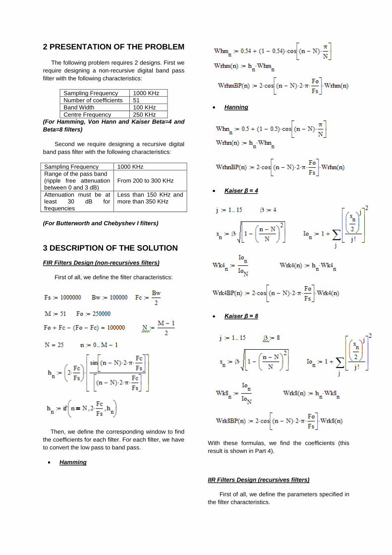
Then, we define the corresponding window to find
the coefficients for each filter. For each filter, we have
to convert the low pass to band pass.
Hamming
Hanning
Kaiser β = 4
Kaiser β = 8
With these formulas, we find the coefficients (this
result is shown in Part 4).
IIR Filters Design (recursives filters)
First of all, we define the parameters specified in
the filter characteristics.
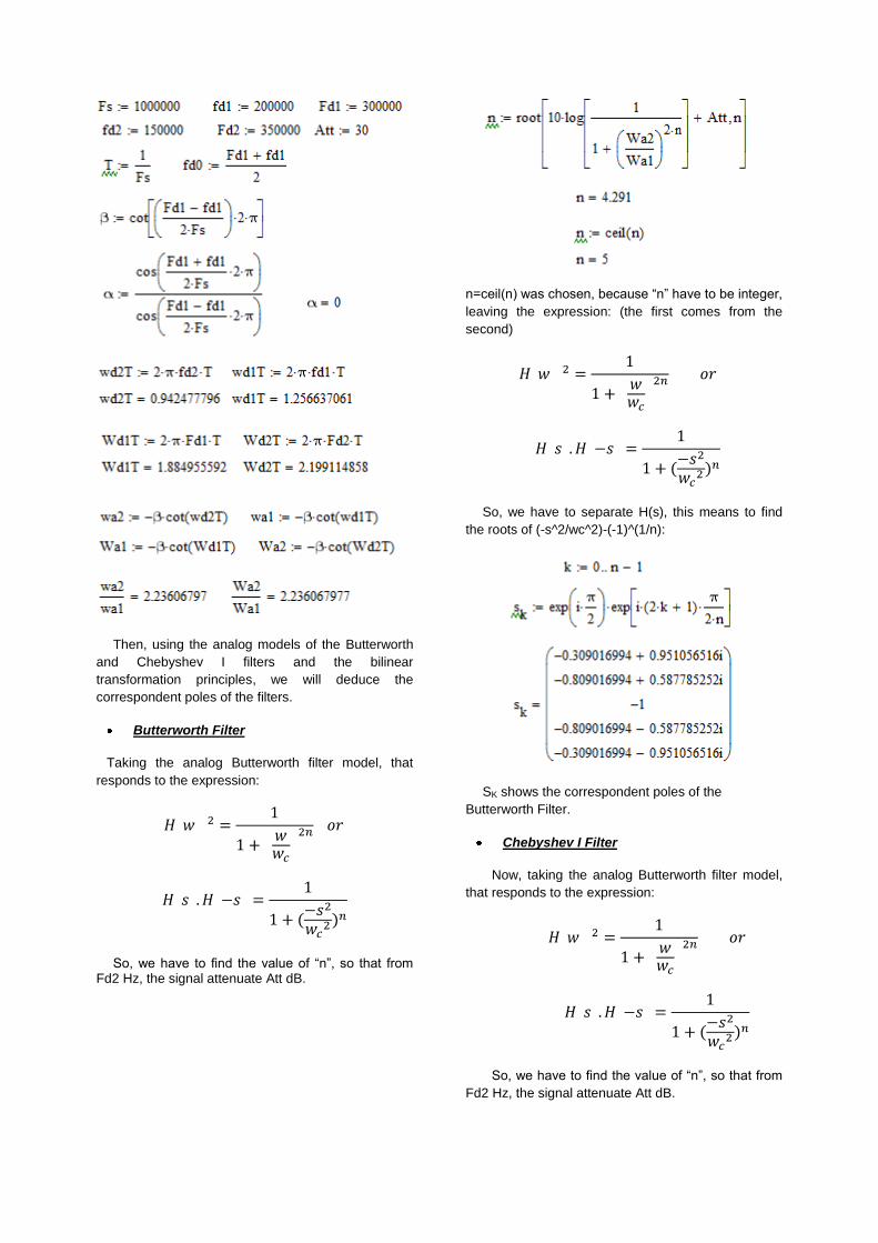
Then, using the analog models of the Butterworth
and Chebyshev I filters and the bilinear
transformation principles, we will deduce the
correspondent poles of the filters.
Butterworth Filter
Taking the analog Butterworth filter model, that
responds to the expression:
So, we have to find the value of “n”, so that from Fd2 Hz, the signal attenuate Att dB.
n=ceil(n) was chosen, because “n” have to be integer,
leaving the expression: (the first comes from the
second)
So, we have to separate H(s), this means to find
the roots of (-s^2/wc^2)-(-1)^(1/n):
SK shows the correspondent poles of the
Butterworth Filter.
Chebyshev I Filter
Now, taking the analog Butterworth filter model,
that responds to the expression:
So, we have to find the value of “n”, so that from
Fd2 Hz, the signal attenuate Att dB.
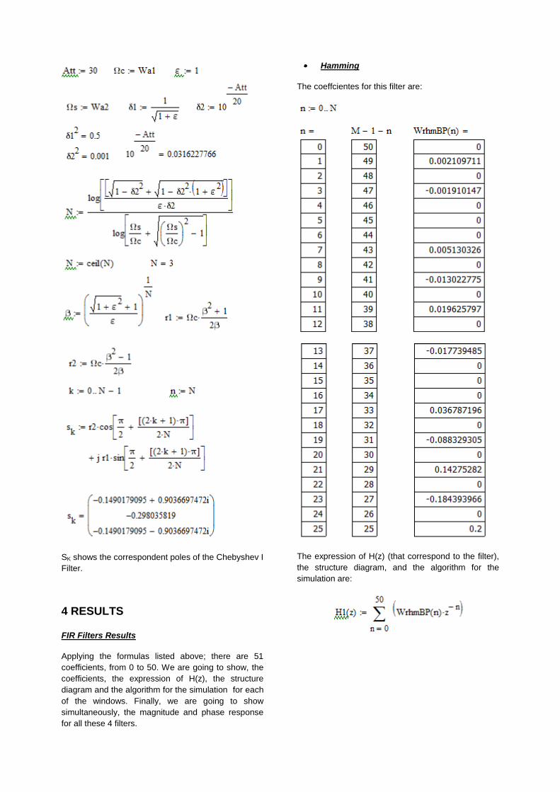
SK shows the correspondent poles of the Chebyshev I
Filter.
4 RESULTS
FIR Filters Results
Applying the formulas listed above; there are 51
coefficients, from 0 to 50. We are going to show, the
coefficients, the expression of H(z), the structure
diagram and the algorithm for the simulation for each
of the windows. Finally, we are going to show
simultaneously, the magnitude and phase response
for all these 4 filters.
Hamming
The coeffcientes for this filter are:
The expression of H(z) (that correspond to the filter),
the structure diagram, and the algorithm for the
simulation are:
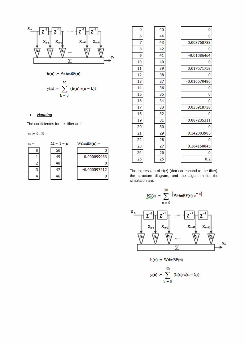
Hanning
The coeffcientes for this filter are:
The expression of H(z) (that correspond to the filter),
the structure diagram, and the algorithm for the
simulation are:
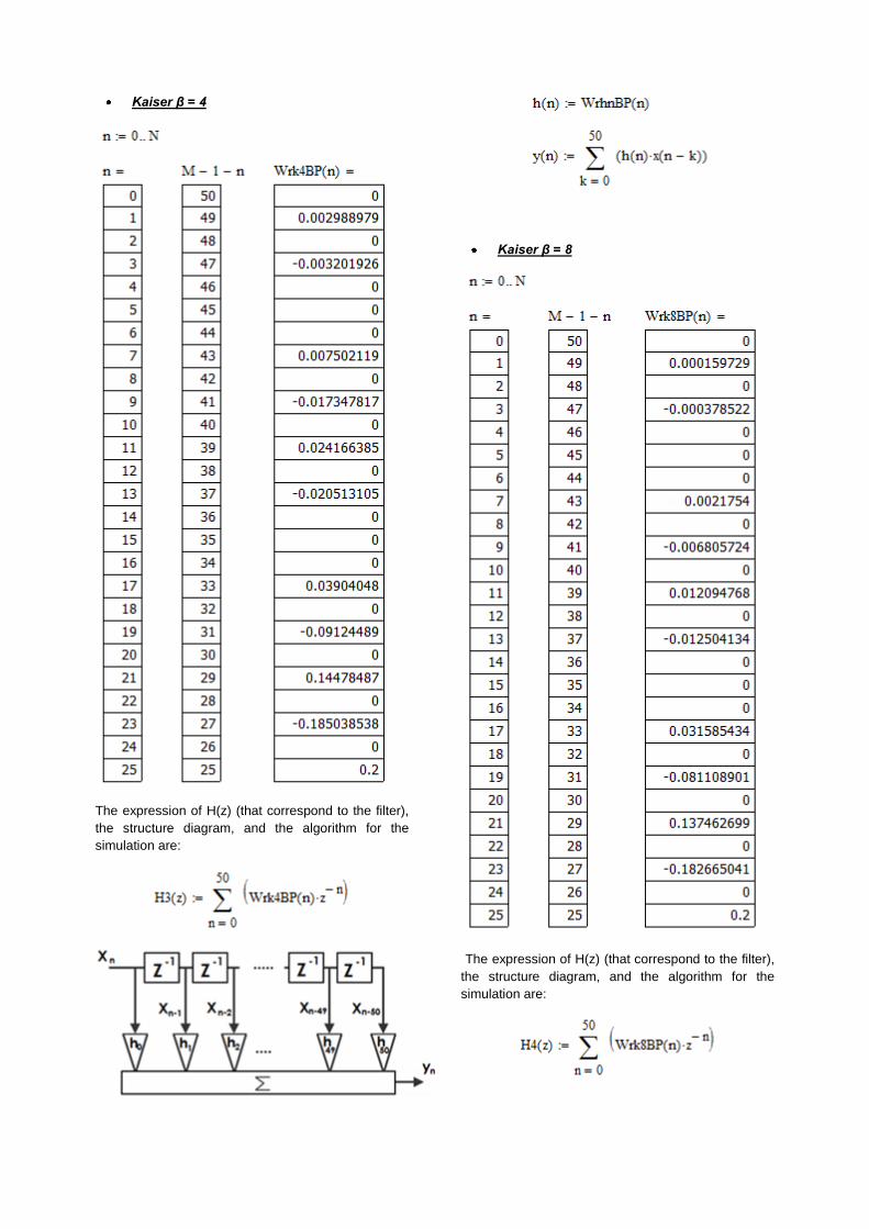
Kaiser β = 4
The expression of H(z) (that correspond to the filter),
the structure diagram, and the algorithm for the
simulation are:
Kaiser β = 8
The expression of H(z) (that correspond to the filter),
the structure diagram, and the algorithm for the
simulation are:
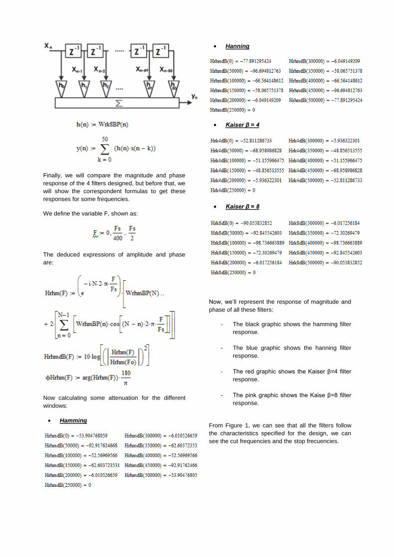
Finally, we will compare the magnitude and phase
response of the 4 filters designed, but before that, we
will show the correspondent formulas to get these
responses for some frequencies.
We define the variable F, shown as:
The deduced expressions of amplitude and phase
are:
Now calculating some attenuation for the different
windows:
Hamming
Hanning
Kaiser β = 4
Kaiser β = 8
Now, we’ll represent the response of magnitude and
phase of all these filters:
- The black graphic shows the hamming filter
response.
- The blue graphic shows the hanning filter
response.
- The red graphic shows the Kaiser β=4 filter
response.
- The pink graphic shows the Kaise β=8 filter
response.
From Figure 1, we can see that all the filters follow
the characteristics specified for the design, we can
see the cut frequencies and the stop frecuencies.
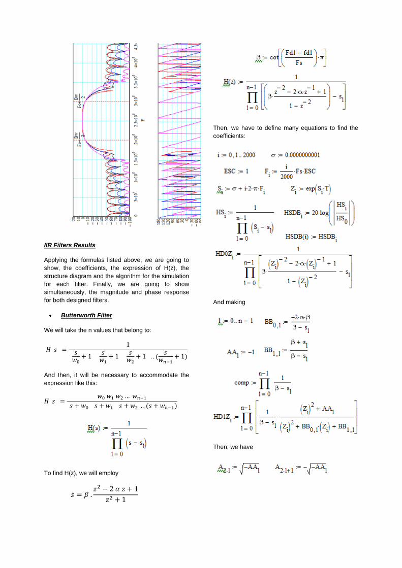
Figure 1. Magnitude and Phase
response for FIR filters
IIR Filters Results
Applying the formulas listed above, we are going to
show, the coefficients, the expression of H(z), the
structure diagram and the algorithm for the simulation
for each filter. Finally, we are going to show
simultaneously, the magnitude and phase response
for both designed filters.
Butterworth Filter
We will take the n values that belong to:
And then, it will be necessary to accommodate the
expression like this:
To find H(z), we will employ
Then, we have to define many equations to find the
coefficients:
And making
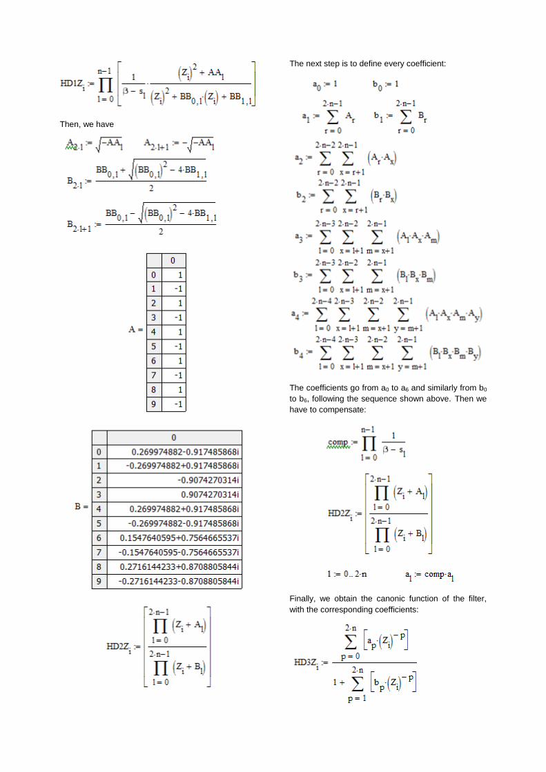
Then, we have
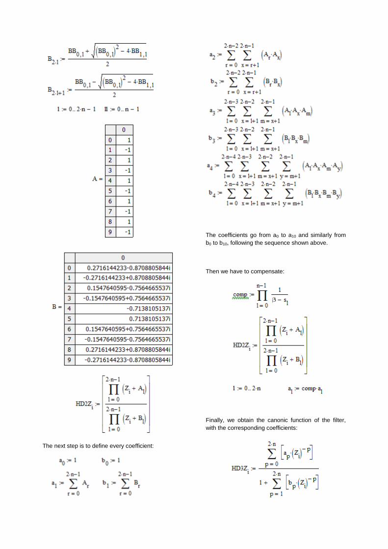
The next step is to define every coefficient:
The coefficients go from a0 to a10 and similarly from
b0 to b10, following the sequence shown above.
Then we have to compensate:
Finally, we obtain the canonic function of the filter,
with the corresponding coefficients:
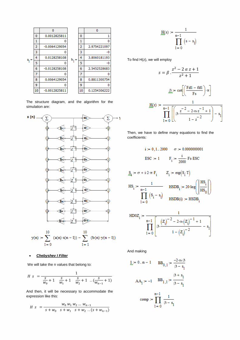
The structure diagram, and the algorithm for the
simulation are:
Chebyshev I Filter
We will take the n values that belong to:
And then, it will be necessary to accommodate the
expression like this:
To find H(z), we will employ
Then, we have to define many equations to find the
coefficients:
And making
Then, we have
The next step is to define every coefficient:
The coefficients go from a0 to a6 and similarly from b0
to b6, following the sequence shown above. Then we
have to compensate:
Finally, we obtain the canonic function of the filter,
with the corresponding coefficients:
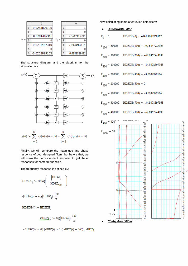
The structure diagram, and the algorithm for the
simulation are:
Finally, we will compare the magnitude and phase
response of both designed filters, but before that, we
will show the correspondent formulas to get these
responses for some frequencies.
The frequency response is defined by:
Now calculating some attenuation both filters:
Butterworth Filter
Figure 2. Magnitude and Phase
response for Butterworth filter (IIR filter)
Chebyshev I Filter
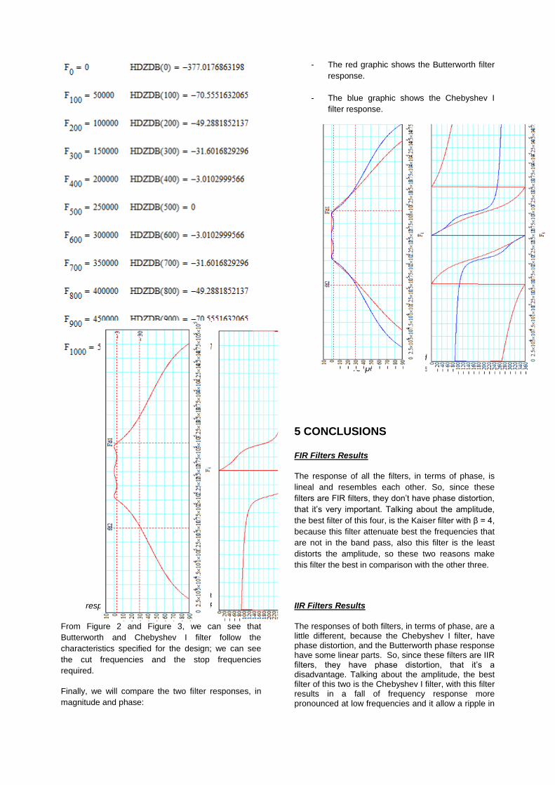
Figure 3. Magnitude and Phase
response for Chebyshev I filter (IIR filter)
From Figure 2 and Figure 3, we can see that
Butterworth and Chebyshev I filter follow the
characteristics specified for the design; we can see
the cut frequencies and the stop frequencies
required.
Finally, we will compare the two filter responses, in
magnitude and phase:
- The red graphic shows the Butterworth filter
response.
- The blue graphic shows the Chebyshev I
filter response.
Figure 4. Magnitude and Phase
response for IIR filters
5 CONCLUSIONS
FIR Filters Results
The response of all the filters, in terms of phase, is
lineal and resembles each other. So, since these
filters are FIR filters, they don’t have phase distortion,
that it’s very important. Talking about the amplitude,
the best filter of this four, is the Kaiser filter with β = 4,
because this filter attenuate best the frequencies that
are not in the band pass, also this filter is the least
distorts the amplitude, so these two reasons make
this filter the best in comparison with the other three.
IIR Filters Results
The responses of both filters, in terms of phase, are a little different, because the Chebyshev I filter, have phase distortion, and the Butterworth phase response have some linear parts. So, since these filters are IIR filters, they have phase distortion, that it’s a disadvantage. Talking about the amplitude, the best filter of this two is the Chebyshev I filter, with this filter results in a fall of frequency response more pronounced at low frequencies and it allow a ripple in
the pass band as shown in the magnitude response above.
In conclusion comparing the two types of filters, after
seeing the magnitude and phase responses, we see
that IIR filters are characterized by greater
attenuation to frequencies that are not in the pass
band, besides the most important feature of these
filters is that the phase response is linear. One
advantage of IIR filters is that we will need smaller
number of coefficients for the specified design
features, but today that’s no problem because the
microprocessor can use a large amount of
coefficients. Then the best option is to use FIR filters.
6 BIBLIOGRAPHY
Books:
<> Digital and Kalman Filtering , S.M. Bozic
England 1994, 2th Edition
[Search: 01 August]
<> Tratamiento Digital de Señales, Proakis
Madrid 2007, 4th Edition
[Search: 03 August]
<> Tratamiento de Señales en Tiempo Discreto,
Oppenheim and Shafer
Madrid 2000, 2th Edition
[Search: 03 August]
Web Pages:
<> Digital Filters. http://cursos.puc.cl/unimit_muc_013-
1/almacen/1242145247_rcadiz_sec1_pos0.pdf
<> www.mathworks.com
<> htttp://focus.ti.com/dsp
<> http://www.dsptutor.freeuk.com/
Magazines:
<> IEEE Transactions on Digital Signal Processing
<> IEEE Transactions on Digital Signal Processing
Magazine
Recommended