DEVELOPMENT OF IMPROVED TRAVELER SURVEY METHODS FOR
HIGH- SPEED INTERCITY PASSENGER RAIL PLANNING
A Dissertation
by
BENJAMIN ROBERT SPERRY
Submitted to the Office of Graduate Studies of
Texas A&M University
in partial fulfillment of the requirements for the degree of
DOCTOR OF PHILOSOPHY
May 2012
Major Subject: Civil Engineering

Development of Improved Traveler Survey Methods for
High-Speed Intercity Passenger Rail Planning
Copyright 2012 Benjamin Robert Sperry
DEVELOPMENT OF IMPROVED TRAVELER SURVEY METHODS FOR
HIGH- SPEED INTERCITY PASSENGER RAIL PLANNING
A Dissertation
by
BENJAMIN ROBERT SPERRY
Submitted to the Office of Graduate Studies of
Texas A&M University
in partial fulfillment of the requirements for the degree of
DOCTOR OF PHILOSOPHY
Approved by:
Chair of Committee, Mark Burris
Committee Members, Luca Quadrifoglio
Cliff Spiegelman
Kyle Woosnam
Head of Department, John Niedzwecki
May 2012
Major Subject: Civil Engineering
iii
ABSTRACT
Development of Improved Traveler Survey Methods for High-Speed
Intercity Passenger Rail Planning. (May 2012)
Benjamin Robert Sperry, B.S., University of Evansville; M.S., Texas A&M University
Chair of Advisory Committee: Dr. Mark Burris
High-speed passenger rail is seen by many in the U.S. transportation policy and planning
communities as an ideal solution for fast, safe, and resource-efficient mobility in high-demand
intercity corridors. To expand the body of knowledge for high-speed intercity passenger rail in
the U.S., the overall goal of this dissertation was to better understand the demand for high-speed
intercity passenger rail services in small- or medium-sized intermediate communities and
improve planners’ ability to estimate such demand through traveler surveys; specifically, the use
of different experimental designs for stated preference questions and the use of images to
describe hypothetical travel alternatives in traveler surveys. In pursuit of this goal, an Internet-
based survey was distributed to residents of Waco and Temple, two communities located along
the federally-designated South Central High-Speed Rail Corridor in Central Texas.
A total of 1,160 surveys were obtained from residents of the two communities. Mixed
logit travel mode choice models developed from the survey data revealed valuable findings that
can inform demand estimates and the design of traveler surveys for high-speed intercity
passenger rail planning activities. Based on the analysis presented in this dissertation, ridership
estimates for new high-speed intercity passenger rail lines that are planned to serve intermediate
communities should not assume that residents of these communities have similar characteristics
and values. The d-efficient stated preference experimental design was found to provide a mode
choice model with a better fit and greater significance on key policy variables than the adaptive
design and therefore is recommended for use in future surveys. Finally, it is recommended that
surveys should consider the use of images of proposed train services to aid respondent decision-
making for stated preference questions, but only if the images used in the survey depict
equipment that could be realistically deployed in the corridor.

iv
To my fiancée Kelli
v
ACKNOWLEDGEMENTS
I would like to thank the chair of my advisory committee, Dr. Mark Burris, for his
guidance and support on the development of this dissertation and for all of his advice during my
time as a graduate student at Texas A&M University. I would also like to thank the members of
my advisory committee, Dr. Luca Quadrifoglio, Dr. Cliff Spiegelman, and Dr. Kyle Woosnam,
for their contributions and for their willingness to serve on my committee.
I would also like to thank my research supervisor at the Texas Transportation Institute,
Mr. Curtis Morgan, for his support and encouragement of my academic pursuits. Other Texas
Transportation Institute employees that contributed to the research associated with this
dissertation include Mr. Trey Baker, Mr. Shawn Larson, and Mr. Jeff Warner. I also wish to
acknowledge the Southwest University Transportation Center for providing funding support for
the research project upon which this dissertation is based.
Finally, I would like to thank my fiancée Kelli, my family, and all my friends in College
Station and beyond for their unwavering support throughout my academic career.
vi
TABLE OF CONTENTS
Page
ABSTRACT .......................................................................................................................... iii
DEDICATION ...................................................................................................................... iv
ACKNOWLEDGEMENTS .................................................................................................. v
TABLE OF CONTENTS ...................................................................................................... vi
LIST OF FIGURES ............................................................................................................... viii
LIST OF TABLES ................................................................................................................ ix
CHAPTER
I INTRODUCTION .......................................................................................... 1
Research Problem..................................................................................... 2
Research Objectives ................................................................................. 5
Dissertation Outline ................................................................................. 5
II BACKGROUND LITERATURE .................................................................. 7
Intercity Passenger Rail Demand Estimation ........................................... 7
Discrete Travel Mode Choice Models ..................................................... 12
Stated Preference Survey Experimental Design ....................................... 16
Survey Design .......................................................................................... 19
Summary .................................................................................................. 27
III RESEARCH METHODS ............................................................................... 29
Research Setting ....................................................................................... 29
Survey Questionnaire ............................................................................... 34
Stated Preference Question Design .......................................................... 36
Visualization ............................................................................................ 42
Sample Size .............................................................................................. 45
Survey Administration ............................................................................. 47
IV PRELIMINARY ANALYSIS ........................................................................ 50
Sample Description .................................................................................. 50
Internet Survey Bias ................................................................................. 54
Preliminary Data Analysis ....................................................................... 57
Summary .................................................................................................. 65
V DISCRETE CHOICE MODEL ANALYSIS ................................................. 67
Preliminary Model Development ............................................................. 68
Community Analysis ................................................................................ 80
Visualization Analysis ............................................................................. 83
Value of Time Analysis ........................................................................... 88
vii
CHAPTER Page
VI CONCLUSIONS AND RECOMMENDATIONS ......................................... 91
Summary of Findings ............................................................................... 91
Recommendations .................................................................................... 94
Future Research ........................................................................................ 95
REFERENCES ...................................................................................................................... 97
APPENDIX A ....................................................................................................................... 107
APPENDIX B ........................................................................................................................ 113
APPENDIX C ........................................................................................................................ 115
APPENDIX D ....................................................................................................................... 116
APPENDIX E ........................................................................................................................ 117
APPENDIX F ........................................................................................................................ 121
APPENDIX G ....................................................................................................................... 123
APPENDIX H ....................................................................................................................... 125
APPENDIX I ......................................................................................................................... 128
APPENDIX J ......................................................................................................................... 134
VITA ..................................................................................................................................... 137
viii
LIST OF FIGURES
Page
Figure 1 Location of Study Communities in Central Texas .............................................. 30
Figure 2 Screen Shot of Typical Stated Preference Question Set ...................................... 42
Figure 3 “Typical” Visualization Package ........................................................................ 44
Figure 4 “Flashy” Visualization Package .......................................................................... 44
Figure 5 Screen Shot of Travel Choices Introduction Screen............................................ 45
ix
LIST OF TABLES
Page
Table 1 Attribute Levels for D-Efficient Stated Preference Design ................................. 39
Table 2 Endpoints of Range of Attribute Levels for Adaptive Design ............................ 40
Table 3 Characteristics of Survey Sample ....................................................................... 51
Table 4 Resident Experience with Rail Transportation Systems ..................................... 53
Table 5 Comparison of Age Group and Household Income ............................................ 55
Table 6 Survey Sample Weights: Waco ........................................................................... 56
Table 7 Survey Sample Weights: Temple ........................................................................ 56
Table 8 Non-Trading and Lexicographic Behavior by Stated Preference Design ........... 58
Table 9 Selected Survey Behavior Measures by Visualization Package .......................... 59
Table 10 Average Attribute Values for Chosen Mode by Visualization Package ............. 61
Table 11 Visualization Effects: Comparison of Text and Images ...................................... 62
Table 12 Visualization Effects: Comparison of Two Image Packages .............................. 63
Table 13 Comparison of Opinion Question Scores by Choice ........................................... 64
Table 14 Factor Analysis of Rail Experience and Resident Opinion Responses ............... 70
Table 15 Comparison of Preliminary Multinomial Logit Model Parameter Estimates...... 73
Table 16 Pooled Model Multinomial Logit Model ............................................................ 75
Table 17 Pooled Model Mixed Logit Model Parameter Estimates .................................... 78
Table 18 Market Segmentation Analysis ........................................................................... 80
Table 19 Final ML Model Parameter Estimates by Study Community ............................. 81
Table 20 Final ML Model Parameter Estimates by Text-Only and Image Packages ........ 84
Table 21 Final ML Model Parameter Estimates by Three Image Packages ...................... 86
Table 22 Value of Time Analysis by Market Segment ...................................................... 89

1
CHAPTER I
INTRODUCTION
High-speed passenger rail is seen by many in the U.S. transportation policy and planning
communities as an ideal solution for fast, safe, and resource-efficient mobility in high-demand
intercity corridors between 100 and 500 miles in total endpoint-to-endpoint length (Federal
Railroad Administration, 2009a; Passenger Rail Working Group, 2007; Peterman et al., 2009).
While this means of intercity travel has been implemented widely and with much success in
Europe and Asia for several decades (Campos and de Rus, 2009), development of high-speed
passenger rail in the U.S. has not realized a similar experience. In the U.S., passenger rail
services in the Northeast Corridor (Washington, D.C. – New York – Boston) can reach up to 150
miles per hour in some places along the line, but average speeds are much lower (Schwieterman
and Scheidt, 2007). Outside of the northeast, although efforts have been on-going for several
decades (Federal Railroad Administration, 1997; Fisher and Nice, 2007), high-speed passenger
rail development has been unsuccessful. Proposals across the U.S. totaling 64 unique intercity
corridors and more than 15,000 miles of route have been identified, including major initiatives in
California, Florida, the Midwest, and the Southeast (Schwieterman and Scheidt, 2007).
However, to date, no high-speed trains have been established outside the Northeast Corridor.
Transportation planning is the branch of transportation engineering that is concerned
with formulating alternative investment strategies to ensure that the transportation system
provides safe and efficient mobility for people and goods within a framework of community
goals. The key output of all transportation planning activities is one or more recommendations
to decision-makers as to the preferred investment strategy that balances transportation system
needs, stakeholder objectives, and scarce public resources available for such investments.
Intercity passenger rail planning encompasses a variety of scenarios, each with varying levels of
complexity and requirements for data to support decision-making. Intercity passenger rail
planning scenarios could include the following (Roth, 1998; Sperry and Morgan, 2010):
Establishing new intercity passenger rail service where none currently exists;
Extending existing intercity passenger rail corridors to new market areas;
This dissertation follows the style of Transportation Research Part A.

2
Expanding of existing service in the form of additional service frequencies;
Expanding of service in the form of additional station stops along the existing route;
Increasing seating capacity; or
Reducing or eliminating of any of the above.
For all these scenarios, a critical element in the decision-making process is the potential demand
for the proposed new services or enhancements to existing service. When establishing new
intercity passenger rail services, ridership forecasts are generally developed in conjunction with
a proposed service plan (e.g. communities to be served, projected travel times, and expected
service frequencies) and used to develop revenue projections, procure appropriate rolling stock,
and design station facilities to the anticipated demand levels. In a similar fashion, ridership
projections are used to identify when and where route expansions or capacity upgrades will be
necessary to match appropriate service levels. Investments in intercity passenger rail are capital-
intensive, with cost estimates ranging from $7 million to $35 million per mile (Peterman et al.,
2009). As a result, ridership estimates (and the corresponding financial projections) with known
levels of accuracy and clearly-articulated uncertainties are desired to move projects forward and
to obtain buy-in from policymakers, investors, and other stakeholders.
RESEARCH PROBLEM
As the nation moves forward with a significant investment in its outdated intercity
passenger rail system, a number of planning and policy barriers exist, making it difficult to fully-
realize the anticipated benefits of high-speed passenger rail (e.g. Federal Railroad
Administration, 2009a; Miller, 2004; Sperry and Morgan, 2010). While some progress has been
made in the form of several new Federal initiatives to jump-start rail projects across the country
(e.g. Federal Railroad Administration, 2009a), there is still much to be learned about the intercity
corridors that have been targeted for high-speed rail investment. To expand the body of
knowledge for high-speed intercity passenger rail planning in the U.S., this dissertation
examined questions in three inter-related areas, as described in the following sections.
Mobility Needs of Intermediate Communities
The first focus area for this dissertation was the demand for new passenger rail service
on small- or medium-sized communities in the intermediate areas between two larger urban

3
areas that form the endpoints of a major intercity corridor. In these communities, where intercity
transportation options may be more limited, the potential development of new intercity
passenger rail lines represents a significant opportunity to realize benefits on a number of fronts.
For example, the improved intercity travel times resulting from new rail services have been
shown to reduce the “functional distance” between these communities and the major endpoint
cities (e.g. Blum et al., 1997; Bonnafous, 1987; Chen and Hall, 2011; Givoni, 2006; Ureña et al.,
2009). This spatial reorganization allows for more long-distance work commuting between
intermediate communities and major endpoint cities, and also serves to improve the
attractiveness of the intermediate community for business travel, conventions and meetings, or
tourism (Ureña et al., 2009). These growth opportunities may not be fully realized if the
alignment of new rights-of-way or train stopping patterns focus on endpoint traffic and neglect
the mobility needs of the intermediate communities (Harrison and Gimpel, 1998). In this classic
transportation issue (balance of mobility needs and access to the transportation system), there is
a need to identify and understand the mobility implications and opportunities that could result
from the development of high-speed passenger rail service in these intermediate communities.
One specific concern relating to the impacts of high-speed passenger rail service in
small- or medium-sized intermediate communities is the need to understand how residents of
such communities might respond to new or upgraded services. To this end, planners develop
ridership models that account for current and future transportation system characteristics as well
as the tastes and preferences of the individual travelers. These models are usually developed
from data obtained from intercept surveys of travelers along major links in an intercity corridor,
which examine potential traveler response to new high-speed rail service. This approach, with
an apparent focus on endpoint-to-endpoint travelers, may neglect the needs, preferences, and
tastes of those who are traveling to or from intermediate communities. As a result, travel
demand model specifications and the resulting parameters (such as a traveler’s willingness to
pay (WTP) for modal attributes such as travel time or travel frequency) may not accurately
reflect the true values for travelers from intermediate communities. In turn, demand estimates
may be skewed due to the use of inaccurate parameters.
Stated Preference Surveys for Demand Estimation
The second focus area of this dissertation examined the methods used by planners to
obtain traveler preference data for passenger rail demand models. Data used to inform

4
transportation planning decisions, including intercity passenger rail planning decisions, can be
described as either “revealed preference” or “stated preference” data (Ortúzar and Willumsen,
2001). For entirely new intercity passenger rail services, or proposed changes to existing lines
where revealed preference data cannot easily be applied, planners rely on data from a stated
preference exercise contained within traveler surveys to develop ridership forecasts. In a stated
preference exercise, the respondent is presented with a number of scenarios in which he or she
will choose their preferred option (or rank their preferences from among several options) from a
set of choices involving different travel options (including future passenger rail) and their
attributes (i.e. travel time, travel cost, and frequency of service). One of the most powerful
features of the stated preference survey technique is the ability of the analyst to arrange the
attributes being considered in the survey in such a way that the responses are elicited in a
controlled manner. This arrangement of the alternatives and attributes is called the experimental
design of the stated preference survey, and a number of experimental design approaches are
available to the analyst (Louviere et al., 2000; Rose and Bliemer, 2008). In an effort to ensure
the most reliable parameter estimates for choice models used in high-speed intercity passenger
rail planning, this dissertation examined the use of different experimental designs in the
development of stated preference exercises for traveler surveys.
Visualization of Travel Alternatives
A second concern related to the design of stated preference exercises for high-speed
intercity passenger rail planning is the realism of the choice context in the exercise. In a stated
preference exercise, the choice context should be as real as possible in order to elicit the most
accurate response (Bradley, 1988). Given that many travelers in an intercity corridor
(particularly outside the Northeast U.S.) may have little or no experience with intercity
passenger rail as a viable travel alternative, it is logical that surveys might use maps or other
images to provide additional context for the decision process. The use of visual material to aid
in respondent decision-making on a stated preference survey is not a new concept (e.g. Carson et
al., 1994) and in fact is highly-recommended to aid respondent decision-making. However, the
impacts of these visual cues on survey outcomes are not well-established in the literature. Two
studies identified in the literature examining this issue (Arentze et al., 2003; Rizzi et al., 2011)
found conflicting results in terms of the impacts of images on stated preference survey outcomes.
Specifically related to high-speed passenger rail, the potential for visualization to bias stated

5
preference survey responses has been raised as an issue for ridership estimation (Roth, 1998).
Given the need for accurate survey responses and the potential influence of visual cues on survey
outcomes, a better understanding of how text or pictorial representation of the travel choices
influences travelers’ intention to utilize proposed new high-speed rail service is desired.
RESEARCH OBJECTIVES
The overall goal of this dissertation was to gain a better understanding of the demand for
high-speed intercity passenger rail services in small- or medium-sized intermediate communities
and improve planners’ ability to estimate such demand through traveler surveys. In pursuit of
this goal, the specific objectives were identified as follows:
Estimate the traveler response to proposed intercity passenger rail service in small- or
medium-sized intermediate communities located in an intercity corridor;
Examine the effects of different stated preference experimental design approaches on the
survey quality and model outcomes; and
Examine the effects of visual supporting material in the description of travel alternatives
in a stated preference survey on the survey quality and model outcomes.
To support these objectives, an Internet-based traveler survey was developed and deployed to
residents of two varying-sized communities in Central Texas which are located in an
intermediate area of the South Central High-Speed Rail Corridor, a federally-designated high-
speed passenger rail corridor which includes the intercity corridor between Dallas-Fort Worth,
Austin, and San Antonio, Texas.
DISSERTATION OUTLINE
After the Introduction, this Dissertation will address the issues of the research problem
through the following chapters: Background Literature, Research Methods, Preliminary
Analysis, Discrete Choice Model Analysis, and Conclusions and Recommendations. A
summary of each chapter is provided below.
Chapter II reviews the relevant Background Literature associated with the research
problem. The review includes an overview of demand estimation for high-speed intercity

6
passenger rail, discrete travel mode choice models, experimental designs for stated preference
surveys, and travel survey design. The literature review raises important issues related to the
treatment of intermediate communities in demand estimation for high-speed intercity passenger
rail service. Additionally, the different experimental designs used in stated preference surveys
for high-speed intercity passenger rail planning are identified. Finally, the visualization of travel
alternatives in a stated preference survey and the impacts of visualization on survey responses in
the context of high-speed intercity passenger rail planning are discussed.
Chapter III, Research Methods, provides the complete details of the setting for the
research, survey questionnaire design, sampling and recruitment, and the administration of the
resident survey used in this Dissertation. The setting for the research was Waco and Temple,
two communities in Central Texas. An Internet-based survey was deployed to residents of these
two communities, including questions about current travel patterns, six stated preference
questions about potential use of intercity passenger rail, and demographic profile information.
Complete details of the stated preference experimental designs and visualization packages used
in the resident survey are also provided in this chapter.
Chapter IV, Preliminary Analysis, provides a description of the survey sample and the
identification of possible bias resulting from the use of the Internet for the survey. Preliminary
analysis of the resident survey examining instances of non-trading and lexicographic behavior in
the data as well as the effects of visualization is also presented.
Chapter V, Discrete Choice Model Analysis, presents detailed travel mode choice
models for various segments of the data based on the research objectives. A pooled choice
model specification is estimated using the mixed logit formulation with a random parameter to
account for multiple observations from a single respondent. Optimal models are fit to each
segment based on study community, stated preference experimental design, and visualization
package. The chapter concludes with a more detailed analysis of the value of time estimated
from each model segment, obtained via simulation.
Chapter VI, Conclusions and Recommendations, provides a summary of the entire
research and identifies the key findings. Recommendations for demand estimation and traveler
survey design for high-speed intercity passenger rail planning are provided and future research
topics are discussed.

7
CHAPTER II
BACKGROUND LITERATURE
The primary focus of this dissertation is to better understand the demand for high-speed
intercity passenger rail services in small- or medium-sized intermediate communities and
planners’ ability to estimate such demand through traveler surveys. As with all research studies,
a detailed understanding of existing research on the topics of interest is a critical first step to
ensure that past findings are acknowledged and to identify the contribution of the proposed study
within the body of knowledge. Topics examined in this literature review include demand
estimation for intercity passenger rail, discrete intercity mode choice models, and survey designs
for intercity passenger rail planning.
INTERCITY PASSENGER RAIL DEMAND ESTIMATION
Previous sections identified some of the key issues that confront the practice of demand
estimation for intercity passenger rail, as well as the importance of obtaining demand estimates
with high levels of accuracy and certainty. This section presents an overview of the general
procedures and data sources used to estimate ridership for new intercity passenger rail services,
both high-speed and conventional.
Typical Estimation Procedure
A number of ridership and revenue studies for proposed high-speed intercity passenger
rail routes that exist in the literature were reviewed to identify the “typical” procedure used to
estimate demand for new services. These studies included Brand et al. (1992), Federal Railroad
Administration (1997), Hensher (1997), Roth (1998), Outwater et al. (2010), and Transportation
Economics and Management Systems, Inc. (2008, 2010). These studies suggest that the typical
demand estimation procedure for new passenger rail service in an intercity corridor generally
consists of the following three steps:
Step 1: Estimate of total travel in the intercity corridor by all existing travel modes for
the current year and projections of the same demand for the target year;
Step 2: Estimate potential diversion of intercity trips from existing modes to the new
passenger rail service; and

8
Step 3: Estimate the quantity of “induced” intercity travel expected to be generated by
the new service.
Summing the outputs from Step 2 and Step 3, the total ridership estimate for a new intercity
passenger rail route is obtained. For Step 1, estimates of current and projected travel by origin
and destination in an intercity corridor are obtained from observed travel patterns and demand
trends, obtained from a variety of sources. This task is particularly difficult for intercity
automobile travel, as typical data sources such as permanent count stations do not identify the
exact origin or destination of the vehicle or the number of occupants in the vehicle. For other
intercity modes, existing travel can be obtained from boarding counts at airports, rail stations, or
intercity bus terminals or through ticket sales data. Ridership estimates for Step 2 are obtained
by applying mode choice models to the projected number of intercity trips to estimate diversion
from existing modes to the new rail service. Diversion models are developed primarily using
survey data obtained from corridor travelers, and are usually specified by mode, segmented by
variables such as trip purpose (generally business or non-business) or trip length (greater or less
than a specified distance). Discrete intercity mode choice models that are developed as part of
Step 2 will be discussed in greater detail in a subsequent section.
Induced Travel
In the final step of the typical ridership estimation process, the amount of induced travel
expected to be generated by the new passenger rail service is estimated. Arguably, induced
travel is a difficult phenomenon to predict, and also could have a significant impact on the
success or failure of a proposed high-speed rail project at the feasibility stage. Passenger rail-
induced travel is classified into four categories (Gunn et al., 1992; Kanafani and Youssef, 1993):
Suppressed Demand: Travel conditions may improve as a result of the introduction of
high-speed rail, and may encourage trips by individuals who did not travel in the past at
all, or those who did not travel for a particular trip purpose.
Increased Propensity: Attributes of the new high-speed rail service may increase the
propensity of current travelers to increase the frequency of their trips, but implies no
change in trip purpose.
Novelty Travel: Curiosity about high-speed rail may lead to one-time trips aimed solely
at experiencing the new mode.

9
Shifting Urban Dynamics: The introduction of high-speed rail may encourage local and
regional development patterns and may allow businesses to seek markets further away
from their location while maintaining links through high-speed rail. The growth of the
impact market region of firms due to high-speed rail also introduces a multiplier effect,
which may stimulate further growth and travel in its local economy.
The consensus among the literature reviewed regarding induced travel is that the percentage of
induced trips attributed to new high-speed rail service is generally a function of the relative rate
of diversion from existing modes. If the diversion rate is high, a new travel mode is expected to
be relatively popular and it is reasonable that there will be induced trips generated as well. A
linear-type relationship between diverted and induced demand was used to estimate induced
ridership for a proposed high-speed passenger rail route between Tampa and Orlando, Florida
(AECOM Consulting and Wilbur Smith Associates, 2002). The California ridership model also
considered the increased accessibility of destinations in the high-speed network as a component
of induced demand (Outwater et al., 2010). As a percentage of total demand, ridership studies
for proposed high-speed rail service around the U.S. have identified induced travel rates between
less than 10 percent to as high as 50 percent (Federal Railroad Administration, 1997).
International experience from the French TGV suggests induced travel on currently-operating
high-speed rail lines can be as high as 49 percent (Bonnafous, 1987). This wide range of
estimated induced travel contribution reflects the challenge and uncertainty of predicting traveler
response to new modal alternatives, particularly the induced component. Challenges associated
with estimating induced travel are noted in the literature, with Gunn et al. (1992) suggesting that
stated intentions methods would overestimate induced travel while Hensher (1997) points out
that surveying current travelers does not allow for an estimate of potential induced travel by
current non-travelers in an intercity corridor.
Implications for Intermediate Communities
The need for adequate transportation facilities as a determinant of a community’s overall
health has long been recognized by transportation planners (see, for example, Clark, 1958). For
decades, intercity travel in the U.S. was operated as a private, for-profit enterprise with extensive
Federal regulations on carrier entry/exit into travel markets as well as fare levels that could be
charged for particular trips. These regulations were designed such that money-making intercity
routes subsidized operations on unprofitable routes, but the carriers as a whole were profitable.
10
This allowed for small- or medium-sized communities of all types to be served by at least some
form of intercity transportation besides the automobile. However, with the nationalization of the
country’s passenger rail service in 1970 and deregulation of the airline (1978) and intercity bus
(1982) industries, intercity carriers were allowed to exit unprofitable markets, leaving many
smaller communities without alternatives to the automobile for intercity travel. Since the mid-
1980s, Federal programs have provided funding for some new intercity services in smaller
communities (Dempsey, 1987; KFH Group, 2002). Furthermore, the importance of current
Amtrak passenger rail service to the communities it serves cannot be understated (Brown, 1997).
Evidence exists in the literature that the methods used to plan for new high-speed
intercity passenger rail services may have significant negative impacts on small- or medium-
sized intermediate communities. At the highest level of planning for new passenger rail
infrastructure, the needs of intermediate communities may be neglected entirely. Policymakers
considering alternatives for the acquisition of the necessary right-of-way for new high-speed rail
lines, for example, could opt for an alternative which results in new lines completely bypassing
intermediate communities in the name of endpoint-to-endpoint mobility. As Harrison and
Gimpel (1998) state about the treatment of potential demand from intermediate communities:
The fundamental issues that determine [High Speed Ground Transportation]
routes are where people are and where they want to go. These endpoints define
the whole exercise of transportation planning and development. Intermediary
points of varying importance and influence will vie for alternative routes or
stations, but an HSGT route cannot compromise its opportunities for
commercial success by ignoring the big market magnets such as downtowns or
airports which invariably tend to define its endpoints (Page 35)…
Perhaps the most important factor [for station location and spacing] is the
travel demand for endpoint markets, and traveler’s willingness to compromise
their travel time objectives (between the major markets) to accommodate the
intermediate transportation needs of short-term travelers (Page 36)…
The sentiment reflected in the comments of Harrison and Gimpel (1998) reflect a post-
deregulation attitude of the mandate for intercity services to generate profits (i.e. “commercial
success”) rather than provide a social good as travel options for intermediate communities.
González-Savignat (2004a) reflects on the potential issue of serving intermediate communities,
11
noting that the existence of intermediate stops is a “very important and controversial planning
service decision” and that “most intermediate communities demand an [high-speed train] stop”
along the Madrid-Barcelona route. In this scenario, planners are trading-off between endpoint-
to-endpoint travel time, travel demand for both endpoint and intermediate cities, and the cost of
right-of-way purchases for either new “greenfield” corridors or existing railroad corridors.
One of the byproducts of the emphasis on endpoint-to-endpoint travel as a major
contributor of demand for new high-speed passenger rail services is evidenced in the growing
body of literature focused specifically on the diversion of existing airline passengers to proposed
rail services (e.g. Buckeye, 1992; Capon et al., 2003; González-Savignat, 2004b; Román et al.,
2007; 2010). Given that the characteristics of high-speed passenger rail and short-haul air carrier
service are similar in terms of both travel attributes and passenger markets served, it is not
surprising that air travel commands such a large attention in the literature. Demand models for
intercity travel developed by Bhat (1995) and Hensher (1997) found that endpoint-to-endpoint
travel (as a dummy variable) was significant in the intercity mode choice model.
Where new high-speed intercity passenger rail lines have been routed to conveniently
serve intermediate communities between major endpoint cities, a number of impacts to the
intermediate communities have been identified in the literature. Most notably, the linkage of
intermediate communities along a major intercity corridor via a high-speed passenger rail line
transforms the corridor into an integrated functional region (Givoni, 2006). Economically, Blum
et al. (1997) identifies the integration of markets for goods and services, labor, and the markets
for shopping, private services, and leisure activities as short-term functional changes that can be
realized. In the medium-term, the “functional distance” between intermediate and major cities
decreases with the provision of high-speed rail service, resulting in the relocation of households
and firms within the corridor (Blum et al., 1997). High-speed trains have also been
demonstrated to support faster economic growth and a better transition to a knowledge-based
economy (Chen and Hall, 2011). New rail services also raise the “image” of intermediate cities,
resulting in new opportunities for tourism and convention marketing, as well as the
redevelopment of city centers around rail stations (Ureña et al., 2009). It has been observed
from case studies in Sweden (Fröidh, 2005) and Spain (Rivas and Fröidh, 2009) that the
relocation of households to intermediate cities, coupled with improved travel times between
these cities and major labor markets in the endpoint cities, has resulted in a large population of

12
travelers utilizing regional high-speed lines for daily commuting purposes. These findings
suggest that the effect of the last category of high-speed passenger rail-induced travel, shifting
urban dynamics, has an important long-term spatial implication for intermediate communities.
Ultimately, decisions about the routing of new high-speed rail lines through or around
intermediate cities will be made by the operator of the new service, in conjunction with policy
makers, transportation planners, ridership and revenue study findings, or political pressure from
local stakeholders. To inform these decisions, ridership models will likely develop demand
estimates for a range of scenarios that incorporate different routing and scheduling options for
intermediate communities, including alternatives where these communities are not served at all.
However, there is evidence from the literature that demand models for intermediate communities
may be different in their specification or parameters than the models for endpoint-to-endpoint
travel segments. For example, the work of González-Savignat (2004a) found that short-distance
travelers from intermediate communities derived a slightly higher value of travel time than long-
distance travelers covering the entire route (Madrid-Barcelona). It was reasoned that the value
of travel time was higher for short-distance travelers because a fixed travel time reduction forms
a larger savings in terms of the proportion of total journey travel time for shorter trips as
compared to longer trips. While this is limited evidence, the findings of González-Savignat
(2004b) do suggest that ridership estimates for travel to or from intermediate cities may need to
be treated separately than endpoint-to-endpoint traffic estimates.
DISCRETE TRAVEL MODE CHOICE MODELS
In the second step of the three-step process used to estimate ridership for proposed high-
speed intercity passenger rail lines, travel survey data are used to develop models of how
travelers might choose their intercity travel mode when the new rail line is fully operational.
These models are referred to as “discrete choice” models because an individual traveler is
modeled as choosing one modal option from a finite set of modal options for their trip. As noted
by Ortúzar and Willumsen (2001), the underlying concept of discrete choice models is that the
probability of individuals choosing a given option is a function of their socioeconomic
characteristics and the relative attractiveness of the option. Furthermore, individuals seek to
maximize their utility (or more accurately, minimize disutility) in their travel choices, including
the travel mode choice – building on the seminal work of McFadden (1974). In discrete choice

13
modeling, utility equations are developed which estimate the total utility of traveling by a
particular mode, given the characteristics of the mode (such as travel time or out-of-pocket travel
cost) and the characteristics of the traveler (such as the number of household autos). Data used
to specify these utility equations are generally obtained from stated preference surveys, which
establish parameters such as a traveler’s willingness to pay (WTP) for modal attributes such as
travel time or travel frequency. To predict the probability of an individual choosing a particular
travel mode, the individual’s utility for that mode is transformed into a probability curve using a
mathematical function such as the logit or probit models (Ortúzar and Willumsen, 2001).
Mathematical Formulation of Discrete Choice Model
The mathematical formulation of the discrete choice model is given as follows, with
notation from Rose et al. (2008). Let j refer to the number of alternatives (travel modes) j = 1,
2,…, J and s refer to the choice task s = 1, 2, …, S faced by the respondent. The utility
possessed by an individual for alternative j in choice task s is denoted by Ujs and is given in (1):
js js jsU V (1)
The utility Ujs consists of two components, the observed component of utility for each alternative
j in choice task s (Vjs) and an error component (εjs) that is unobserved by the analyst. The
observed component of utility is assumed to be a linear additive function of several attributes
with corresponding weights. These weights are the unknown parameters to be estimated. We
distinguish between parameters that are equal across all alternatives J (known as generic) and
parameters that are specific to a particular alternative j (known as alternative-specific). Let
denote the parameter weights for the generic parameters k = 1, …, K* and
denote the
parameter weights for the alternative-specific parameters k = 1, …, Kj. The attribute levels for
the generic and alternative-specific parameters are given by and xjks, respectively, for each
choice task s. The observed component of the utility given in Eq. (1) is given by (2):
*
* *
1 1
jKK
js k jks jk jks
k k
V x x
, 1,...,j J , 1,...,s S (2)
Typically, the unobserved error component (εjs) is assumed to take a distribution that is
independently and identically Type I extreme value, allowing for this term to drop out of

14
Equation (1). Therefore, the probability of an individual choosing alternative j in choice set s
given by Pjs and assumes the form of the multinomial logit model given by (3):
1
exp( )
exp( )
js
js J
is
i
VP
V
, 1,...,j J , 1,...,s S (3)
The total number of parameters to be estimated in (2) is given by (4) as follows:
*
jjK K K (4)
The typical method for estimating the parameters (β*
k, βjk) is to identify parameters such that
their log-likelihood function is maximized. Assuming a single respondent with yjs equal to one if
alternative j is chosen in task s and zero otherwise, this function is given in (5):
*
1 1
( , )S J
js js
s j
L y P
(5)
Eq. (5) provides the maximum likelihood estimates for the parameters (β*k, βjk). For the true
values of the parameters (denoted as ( , )) and M observationally identical respondents, it
has been shown that the ML estimates of (β*k, βjk) are asymptotically normally distributed with
mean and an asymptotic variance-covariance (AVC) matrix Ω equal to the negative inverse of
the Fisher information matrix, given by (6):
12 *
1* 1 ( , )
( , )L
IM
(6)
The AVC matrix is a square matrix of dimension x .
Intercity Rail Mode Choice Models
Discrete mode choice models are also used for high-speed intercity passenger rail mode
choice forecasting. An excellent review of 26 such modeling efforts by Capon et al. (2003)
identified several trends regarding discrete choice models for high-speed rail:
Modes Covered: Models either included all potential travel modes in an intercity
corridor or focused on the interaction between proposed high-speed rail and a specific
15
mode such as air carrier. It is noted that the comparison between the demand for high-
speed rail and air travel for short trips was the topic of interest for Capon et al. (2003).
Model Forms: Models were drawn primarily from the logit family, with the binary
model used if only two modes (proposed high-speed rail and an existing mode) were
modeled, and the multinomial model if all modes were considered. To relax the
assumption of the independence of irrelevant alternatives property of the multinomial
logit model, nesting was used in nearly half of the models reviewed. Utility functions
were generally linear-additive but some Box-Cox transformations were also identified.
Modal Attributes: All models reviewed included travel time and travel cost as attributes.
Regarding travel time, models split travel time into in-vehicle or out-of-vehicle
components, or other components such as waiting time or transfer time. Frequency of
rail service was also included in more than half of the models examined.
It is interesting to note that the review of high-speed intercity passenger rail demand models by
Capon et al. (2003) did not include a single model examining passenger rail demand in a U.S.
intercity corridor. As previously mentioned, efforts to establish new high-speed rail in the U.S.
can be traced back to the 1960s (Schwieterman and Scheidt, 2007), with modern efforts outside
the Northeast Corridor starting in the early 1990s. In general, treatment of proposed U.S. high-
speed intercity passenger rail corridors in the academic literature is limited to topics such as the
economic evaluation of proposed high-speed rail lines (e.g. Brand et al., 2001; Levinson and
Gillen, 1997). Notable exceptions are Brand et al. (1992) and Outwater et al. (2010). Brand et
al. (1992) described the ridership estimation process used primarily by consultants in demand
estimation for proposed high-speed intercity passenger rail systems in Florida and Texas in the
early 1990s. Brand et al. (1992) also reported estimated values of travel time and elasticities for
these studies, but additional details of the model attributes and specifications were not included.
Outwater et al. (2010) report on the development of a statewide interregional travel model for
proposed high-speed passenger rail in California. Outwater et al. (2010) describe the creation of
a series of models relating accessibility, destination choice, trip frequency, access and egress
mode, and main intercity travel mode. Outside of these two papers, most details about demand
models for proposed U.S. corridors are found in the myriad of ridership studies that have been
conducted across the country. Most details are limited owing to the proprietary nature of large-
scale modeling efforts, which are valuable intellectual property for their owners.
16
STATED PREFERENCE SURVEY EXPERIMENTAL DESIGN
The use of stated preference experiments in transportation planning and modeling
applications is extensive (see Bliemer and Rose, 2011), for a recent review of applications in the
past decade). Stated preference surveys are useful when the effects of highly-correlated
variables are difficult to observe in actual situations (i.e. as revealed preference data), or if an
estimate of the effects of a new travel mode or other hypothetical transportation system change is
desired. It is in the latter context that stated preference surveys are useful for intercity passenger
rail planning (Fowkes and Preston, 1991; Hensher, 1997; Loo, 2009; Roth, 1998).
In a stated preference or stated choice experiment, the respondent is faced with a
specified number of choice situations in which he or she will choose their preferred option (or
rank their preferences from among several options) from a set of choices involving different
travel options (including future passenger rail) and their attributes (i.e. travel time, travel cost,
and frequency/headway of service). Each attribute has two or more values known as attribute
levels. The arrangement and presentation of the alternatives, attributes, and levels is known as
the “experimental design” of the stated preference survey. A number of experimental designs
are available to the analyst (Louviere et al., 2000; Rose and Bliemer, 2008); a discussion of
several popular design approaches is provided in the following sections.
Factorial Designs
The most basic experimental design for stated preference surveys is known as the
factorial design. A full-factorial design consists of all possible combinations of the levels of the
attributes. For example, if a stated preference experiment consists of three attributes with three
levels each and two attributes with four levels each (denoted as 334
2), there are (3 x 3 x 3 x 4 x 4)
432 unique choice sets that could be presented to a respondent (Kuhfeld, 2010). In a perfect
situation, each respondent would consider all these choices. The resulting data would allow the
analyst to estimate the main effects, as well as both two-way and higher-order interactions
among each of the attributes in a model. However, since it is not practical to present respondents
with all the possible choice sets (except for the most basic of surveys), an alternative to the full-
factorial design, the fractional factorial design, can be used. With the fractional factorial design,
the analyst uses a fraction of the choice sets available from the full-factorial design, with the
trade-off that not all cross-attribute interactions can be estimated in a model. With the fractional
factorial design approach, the analyst selects subsets of the full-fractional choice sets to present
17
to respondents. One way to select these subsets is to randomly select a specified number of sets
to be used. Another way to select subsets is to identify subsets that provide attribute balance
(each attribute level occurs equally often within an attribute) or subsets that are orthogonal (each
pair of attribute levels occurs equally often within all attribute pairs). Orthogonal designs can be
created manually, developed using reference tables, or by using computer macros or specially-
designed software programs (Bliemer and Rose, 2009).
Emergence of Efficient Designs
Despite the widespread use of orthogonal fractional-factorial experimental designs, there
is a growing body of literature that questions the use of such designs for the development of
choice models, including travel mode choice models (e.g. Bliemer and Rose, 2009; Huber and
Zwernia, 1996; Sándor and Wedel, 2001). The motivation for this criticism is rooted in the fact
that the choice models estimated from stated preference data are inconsistent with the orthogonal
methods used to develop the experimental design to collect stated preference data. As a result, a
new class of experimental designs, efficient designs, has emerged in practice. The main
objective of efficient designs is to minimize the AVC matrix (Equation 6) of the underlying
econometric model. Since the square root of the diagonal elements of the AVC matrix are the
asymptotic standard errors of the resulting model, minimizing the AVC matrix elements will, by
default, minimize these errors (Bliemer and Rose, 2009). If the analyst has any prior information
about the values of the model parameters (even just a sign), the AVC matrix of the choice model
can be estimated before the stated preference survey is deployed.
Given the assumed AVC matrix from the prior parameters data, the analyst can derive a
variety of measures of statistical “efficiency” of a proposed experimental design. The most
widely-used measure is known as the D-error because it utilizes the determinant of the AVC
matrix (Kuhfeld, 2010). Mathematically, the D-error is given by (7) as follows:
D-Error = 1
det( ) K (7)
Depending on the level of information available on the prior parameter estimates, different types
of D-error are used (Bliemer and Rose, 2009). Given that the design with the lowest possible D-
error may be difficult to find (recall that the analyst is selecting from a potentially vast number
of potential attribute and level combinations), the phrase D-efficient is used to describe
experimental designs with sufficiently-low D-error (Bliemer and Rose, 2009).

18
Adaptive Designs
Adaptive stated preference designs are an alternative, non-experimental, approach to
fractional, orthogonal, or efficient stated preference designs. Adaptive stated preference surveys
differ from these other designs in that the attribute levels presented to the respondent in
individual choice sets depend upon the responses given to prior choice sets in the same survey
(Richardson, 2002). The phrase “adaptive” in this context does not refer to the common practice
of using revealed preference information to “customize” the stated preference questions to
individual respondent experiences (e.g. Rose et al., 2008). Rather, the approach is “adaptive” in
the sense that the attribute levels presented to the respondent in a given stated preference
question are selected using a method that “adapts” to responses that were given in a prior stated
preference question. The main benefit of using an adaptive approach to stated preference
surveys is that this approach allows the analyst to estimate the exact value that each respondent
attaches to each attribute of interest (Fowkes, 2007; Richardson, 2002; Smalkoski and Levinson,
2005; Tilahun et al., 2007). A secondary benefit of adaptive stated preference questions is that
they allow for the presentation of choices that the individual respondent might actually consider
while removing alternatives that the respondent will not consider (Tilahun et al., 2007). Because
the approach can estimate traveler valuations at the individual traveler level (i.e. disaggregate),
more information per respondent is typically obtained and fewer samples are required. The use
of adaptive stated preference in transportation has been used in a variety of contexts. Smalkoski
and Levinson (2005) and Fowkes (2007) used adaptive stated preference methods to estimate
value of time for freight operators in Minnesota and the United Kingdom, respectively. A
simulation study of value of time by Richardson (2002) found that the adaptive stated preference
approach could reproduce unbiased estimates of the underlying distribution of value of time for a
population. Tilahun et al. (2007) used an adaptive stated preference survey to measure valuation
of bicycle facility type among bicycle commuters in Minnesota. Patil (2009) used an adaptive
design to measure the value of travel time savings for managed lane users in Houston, Texas,
and found that the adaptive design outperformed the efficient design in such estimates.
Experimental Designs used in Intercity Passenger Rail Planning
In intercity corridors where new high-speed passenger rail service (or a significant
upgrade to existing services) has been proposed, a stated preference survey must be used to
measure potential traveler response to the new services. The literature on stated preference
19
surveys for intercity passenger rail planning reveals that the primary experimental design
approach appears to be the commonly-used fractional factorial technique. The use of this
traditional experimental design technique was noted in high-speed passenger rail studies in
Australia (Hensher, 1997; 1998; Johnson and Nelson, 1998), Korea (Wen and Lin, 2007), and
Spain (González-Savignat, 2004a; 2004b; Román et al., 2010). One study, Carlsson (2003),
reported the use of the emerging D-efficient experimental design technique in a study of the
demand for high-speed intercity passenger rail among business travelers in Sweden. Román et
al. (2010), while not having used the D-efficient experimental design in their study of
competition between high-speed rail and airplane in the Madrid-Zaragoza-Barcelona (Spain)
corridor, acknowledged that the use of the main effects fractional factorial experimental design is
not entirely suitable for the estimation of nested logit models, indirectly supporting the need for
the D-efficient design in future studies. Because of its lack of widespread use in stated
preference surveys, no studies were identified that reported the use of the adaptive design
approach for intercity rail planning. The issues previously raised with respect to U.S. modeling
efforts extends to the experimental design discussion, as no U.S. ridership studies examined have
identified the design approach used to develop the stated preference survey used in their studies.
SURVEY DESIGN
It is widely acknowledged that a well-designed survey instrument is critical for the
overall validity of the resulting analysis, and extensive research has been undertaken to improve
the design and implementation of traveler surveys. The literature summarized in this section
examines stated preference surveys; specifically, the potential for bias in such surveys and the
use of visualization of the attributes or alternatives in such surveys. Synthesizing the literature
on stated preference survey quality and the use of visual aids in the survey process, a potential
opportunity for hidden bias emerges. The section concludes with a brief discussion of the
Internet as an emerging medium for traveler surveys.
Survey Quality
In transportation surveys, the quality of the survey data affects the quality of the analysis
or models that are constructed from it. Traditional measures of the quality of traveler surveys,
such as non-reporting or item non-response are well-documented in the literature (e.g.
Richardson et al., 1995). The concern in the proposed research is the stated preference element
20
of traveler surveys. Beyond traditional measures of survey quality, there are quality issues
related specifically to stated preference surveys that are important considerations for the design
of surveys and interpretation of the data.
One of the most important considerations in the context of stated preference data is the
potential for bias to appear in the survey responses. Fowkes and Preston (1991) identify three
types of bias that may affect the quality of stated preference survey data, with specific
considerations for intercity passenger rail planning:
Self-Selectivity Bias: Households or travelers that are more likely to use proposed or
improved passenger rail services are more likely to complete the survey, as there is more
incentive for them to do so;
Non-Commitment Bias: Since there are no real trade-offs being considered in the stated
preference exercise (i.e. respondents are not spending “real” money), respondents may
state that they will utilize new passenger rail services; in reality, for a number of reasons,
they might not behave as the stated preference survey predicted they might; and
Policy Bias: Also known as “strategic bias,” policy bias occurs when respondents
answer in a particular way in order to achieve some desired policy response; in this case,
either to support or oppose the development of new intercity passenger rail services.
Given the importance of stated preference data in major investment decisions, it is desirable to
minimize all types of bias in the survey responses or, at a minimum, be able to detect biased data
and eliminate these responses from subsequent modeling or analyses. The issue of non-
commitment bias, that is to say, respondents “doing what they said they would do,” is difficult to
assess. One issue in detecting non-commitment bias is that the hypothetical situation(s) which
the respondent considered in surveys may not ever be offered or built. Another issue is that even
if the change is ultimately adopted, adequate resources to conduct a suitable formal study (likely
requiring panel data) may not be available. As a result, there is little or no ability for planners to
“check their work” comparing estimated versus actual demand in the name of improving demand
estimates for future projects.
Growing on the notion of policy or strategic bias in stated preference data, a number of
considerations are raised in the literature. Concerning the theoretical link between stated
intention and actual behavior, Fujii and Gärling (2003) noted that strategic responding in an
attempt to exert influence toward a desired end is one of several causes of intention-behavior

21
inconsistency. One example of concerns about policy bias in stated preference data is in the
context of controversial initiatives such as tolling or pricing (e.g. Calfee et al., 2001; Iragüen and
Ortúzar, 2004). In such cases, respondents may answer strategically (i.e. against potential road
pricing initiatives) even in the face of a “controversial” alternative providing the respondent with
the highest utility. Fowkes and Preston (1991) noted that policy bias in rail surveys could be
avoided by attempting to disguise the nature of the survey, although they acknowledged that due
to the promotion of the project by sponsors, politicians, and local media, completely disguising
the nature of a survey is not feasible. Finally, in the context of potential policy bias in rail
passengers’ valuation of premium rolling stock, Lu et al. (2008) noted that the use of a “cheap
talk” script in advance of the stated preference questions appeared to counter of the instances of
strategic bias without making the choice task more difficult.
In light of these potential issues, three specific indicators have been suggested in the
literature that can aid in the interpretation of the quality of stated preference survey data: non-
trading, lexicographic behavior, and inconsistent behavior (Hess et al., 2010). Non-trading
refers to the situation where a respondent always chooses the same alternative regardless of the
attribute and level combinations presented in the choice sets. Non-trading can be a legitimate
outcome of the stated preference exercise (in the case of an individual’s extreme preference for a
particular alternative), but can also reflect respondent fatigue (simply selecting the same
alternative in each choice set) or a policy bias (strong favor or opposition toward a particular
alternative). Lexicographic behavior occurs when a respondent selects alternatives on the basis
of a subset of attributes listed in the choice set (Blume et al., 2006, Hess et al., 2010;
Sælensminde, 2002). For example, if a respondent always chooses the fastest or the cheapest
option, this respondent could be engaging in lexicographic behavior. However, much like non-
trading, lexicographic behavior could be the result of legitimate decision processes on the part of
the respondent. The final indicator is known as inconsistent behavior (Sælensminde, 2001),
whereby a respondent does not appear to behave rationally in the choice experiment. A simple
example of such behavior is when a respondent is willing to accept a particular alternative at a
given marginal cost but is unwilling to accept a lower marginal cost in subsequent choice sets.
Collectively, non-trading, lexicographic behavior, and inconsistent behavior are indicators that
can be used to detect potentially-erroneous stated preference survey responses. If such responses
are identified, the analyst should remove them from the analysis in order to ensure that the model
parameters and WTP values reflect true respondent decision-making processes.
22
Visualization
The quality of the data obtained from a stated preference survey is related to a number of
factors, one such factor being the level of “realism” in the stated preference exercise. Since
stated preference surveys are commonly undertaken to study a hypothetical product or travel
alternative, designers typically wish to include as much information as possible to aid the
respondent in understanding the choice task. The main motivation for improving the realism of
the exercise is to reduce respondent burden, which in turn improves both the quantity and the
quality of the responses. To this end, some literature (e.g. Bradley, 1988; Carson et al., 1994)
suggests the use of visual representations of attributes or alternatives in a stated preference
survey to supplement verbal or written descriptions. The following benefits of including
pictorial representations of attributes or alternatives in choice experiments have been identified
in the literature (Bradley, 1988; Green and Srinivasan, 1978; Jansen et al., 2009):
Certain attributes or alternatives may be difficult to describe with text descriptions;
Visualization may improve comprehension and understanding of the choice task by
reducing information overload, resulting in better choices;
Visualization may lead to higher perception homogeneity because images may be open
to less individual interpretation than written descriptions; and
The choice task may be more interesting or less fatiguing to respondents.
The use of visual representations of attributes is used extensively in new consumer product
marketing, and studies have shown that the visualization improves the accuracy of product
acceptance models (Vriens et al., 1998). Carson et al. (1994) cited the use of videotaped
representations of attribute combinations in choice sets by Anderson et al. (1993) as an example
in practice. Other examples of visual material in stated preference surveys found in the literature
include a study of preferences for residential building types and styles in The Netherlands
(Jansen et al., 2009) or tourists’ choice of destinations for state parks (Louviere et al., 1987).
The use of visual material to add realism to the stated preference exercise in
transportation applications appears to be fairly standard practice, particularly for complex
situations. In this case, visual material in the name of improved realism is designed to aid the
respondent in understanding the choice task. For example, Iragüen and Ortúzar (2004) used
images of particular street features in a stated preference survey of the WTP for reducing
accident risk on urban streets. In another example, Tilahun et al. (2007) used images and videos
23
to portray different options for off-road paths or on-road bicycle lanes to respondents. In these
applications, the common phrase “a picture is worth a thousand words” would be appropriate to
describe the motivation for adding images to the survey.
However, research into the specific effects of incorporating visual material to add
realism to stated preference exercises for travel mode choice models has been fairly limited.
Two studies identified in the transportation literature which specifically examined the impacts of
adding pictorial or visual information to an attribute profile are Arentze et al. (2003) and Rizzi et
al. (2011). In Arentze et al. (2003), the purpose of the study was to improve the quality and
validity of stated choice data from respondents with limited literacy skills. They developed a
mode choice model for commuters in the Pretoria, South Africa region containing train, bus, and
minibus as alternatives. They found that the use of pictorial material supplementing a verbal
description of attributes had no impact on the error variance (p=0.215) or measurement of
attribute weights (p=0.331). Consequently, they concluded that the effort necessary to develop
and present pictorial material was not compensated by better quality data. In Rizzi et al. (2011),
the authors examined how displaying images of heavy traffic congestion during a stated
preference survey affected the value of travel time savings (VTTS) estimated from the resulting
mode choice model. Specifically, given that many stated preference surveys desire to estimate
VTTS for free-flow traffic conditions and congested traffic conditions separately, they
speculated that the inclusion of images would aid the respondent in understanding the context of
“congested” traffic conditions and thus would provide a better estimate of the congested VTTS.
They found that, for the survey respondents who were presented with images, the free-flow
VTTS was $5.70 per hour and the congested VTTS was $7.40 per hour. However, for the
survey respondents without images, the free-flow and congested VTTS were approximately
equal to $5.90 per hour. The conclusion from Rizzi et al. (2011) was that including the traffic
images in the stated preference survey can “substantially influence how traffic conditions
associated with hypothetical travel times are perceived,” as evidenced by the VTTS differences.
The use of visualization of attributes or alternatives in the context of stated preference
surveys for passenger rail planning also appears in the literature, although far less common.
Since the proposed rail service is the hypothetical alternative in a stated preference survey,
providing respondents with some visual material describing the proposed rail service has been
mentioned in the literature. In a survey supporting the design of a very fast train (VFT) system
24
in Australia, Gunn et al. (1992) reported providing the respondent with a “realistic brochure
describing the VFT service, including a route map, a timetable, a picture of the train, and a
description of some service features.” In their questionnaire design, Gehrt and Rajan (2007)
reported providing the respondent with “color photos of the exterior and the interior of an HSR
train” with the intention of making the response setting “more tangible” to respondents. Survey
documentation for the proposed California high-speed rail system utilized a map of the proposed
route to aid respondents in completing the survey (Corey, Canapary, & Galanis Research, 2005).
Hidden Policy Bias?
The use of visual material in traveler surveys appears to be typical practice in situations
where survey designers perceive the need to support the text or verbal survey content with
pictures or images. For example, given that potential travelers in U.S. intercity corridors may be
unfamiliar with the qualitative attributes of Asian- or European-style high-speed passenger rail,
the use of visual material describing these attributes may be helpful for respondents to better-
understand the hypothetical travel context of a proposed passenger rail service. However, the
use of such material in the presentation of the attributes or alternatives (specifically, a pictorial
representation of the proposed high-speed passenger rail service travel alternative) may
effectively bias the stated preference survey data. As Roth (1998) notes:
However, the way in which new [high-speed rail] services are presented must be
carefully considered. Even with a simple and clear presentation, there is likely
to be a certain amount of “justification bias” – the tendency for respondents to
stick with their present mode choice regardless of the attributes of competing
alternatives. On the other hand, if the presentation is rather flashy and its
features overly stressed, an opposite “policy bias” may be created (Page 58).
In the case of the last sentence in the above quote, Roth (1998) suggests that the policy bias
created by the visual presentation of the hypothetical high-speed passenger rail alternative could
serve to overstate the potential use of new rail services. A similar issue was raised in a report on
the development of a traveler survey for the proposed California high-speed rail system by
Botimer et al. (1994). In their discussion of the use of stated preference questions and data in the
survey, they noted the following concern about respondent experience with passenger rail and
potential for bias:
25
Of those respondents who have taken interregional train voyages, many are
likely to have taken them abroad. All respondents who have ridden high speed
rail trains have done so abroad. The underdeveloped nature of the passenger
rail system in the United States, and especially in the West, makes a discussion
of the relative preference of rail service based upon perceptions references to
the European or Japanese rail system likely to introduce significant bias as well.
For instance, people who have traveled extensively in Europe using the greatly
interconnected passenger rail system may mistakenly attribute the
characteristics of such a rail system to the proposed system that is currently
being evaluated in California (Page 158).
Theoretically, the inclusion of strategically-selected images presenting a “flashy” new alternative
travel mode in the survey impacts the survey by incorporating additional information in the
choice process, thereby diverting at least a portion of the respondents’ focus away from trading-
off between the actual attributes considered in the survey. On the surface, this appears to be an
overly skeptical position – after all, all surveys are designed with the full-faith assumption that
the responses provided reflect legitimate and honest decision-making processes on the part of
respondents who consider only the questions given and are not distracted by “noise” on the
survey instrument. However, surveys that include visual aids for survey respondents with no
intention of biasing the resulting data may do more harm than good by including visual material
which might compel responses in a particular direction. Alternatively, visual material may
reduce the variability in the data by providing all respondents with the same representation of a
hypothetical scenario, rather than forcing respondents to create such representations individually.
At a minimum, the true effects of adding such material are not fully understood by planners.
Internet-Based Travel Surveys
The Internet as a prominent tool for intellectual, economic, and social exchange has
emerged in nearly every facet of modern global culture. Survey researchers have embraced this
shift by adopting the medium for survey-based data collection. The benefits of using the Internet
as a medium for survey questionnaires and data collection are summarized as follows (Alsnih,
2006; Couper, 2008; Dillman, 2007):
Low distribution and retrieval costs;
Automated data entry;
26
The ability to include visual aids and animation to assist in the respondent’s completion
of the survey tasks;
Quick response times;
Streamlining of advanced survey features such as skip patterns or randomization of
questions such that the respondent is not aware of these features’ presence; and
The ability to obtain information about response behavior such as response times.
Because of these benefits, Internet-based surveys have expanded rapidly in the last decade
(Couper, 2008), and a number of excellent references have been published, including Couper
(2008) and an extension of the “tailored design method” for survey questions for the Internet by
Dillman et al. (2009). In many respects, Internet surveys are similar in functionality to
computer-assisted phone interview (CAPI) methods (Iragüen and Ortúzar, 2004).
Given the benefits of Internet-based surveys, it is not surprising that transportation
planners and analysts have adopted the medium as well. For household travel diary-type
surveys, for example, Internet-based applications have emerged which allow for interactive
responses, multi-session completion of the survey questionnaire, and the link between GPS
device data and survey questions (Adler et al., 2002; Alsnih, 2006). The Internet has also been
used for specialized surveys such as transit customer satisfaction panels (Spitz et al., 2004),
bicycle commuting studies (Stinson and Bhat, 2004; Tilahun et al., 2007), or household
preferences for clean vehicles (Potoglou and Kanaroglou, 2007). A study of WTP for reducing
fatal accident risk in urban areas (Iragüen and Ortúzar, 2004) highlights several benefits of
Internet surveys for stated preference applications, including the ability to randomize blocks and
choice sets. A stated preference survey of bicycle route alternatives by Tilahun et al. (2007)
utilized an “adaptive” algorithm that allowed for subsequent questions to be displayed based on
prior responses. To the author’s knowledge, the use of Internet-based travel surveys for
ridership studies of proposed high-speed intercity passenger rail routes is limited. Gunn et al.
(1992) speculated that rail surveys could benefit from computer-based interview technology and
the Internet medium was considered in the case of the California high-speed rail project
(Cambridge Systematics et al., 2005). Ridership models for a privately-financed high-speed rail
line connecting Las Vegas, Nevada and Victorville, California, were developed using data
obtained from an Internet-based survey panel of selected Southern California residents who were
considered potential passengers of the new service (Cambridge Systematics, 2008).
27
In spite of the benefits of Internet-based surveys, there are serious concerns about the
representativeness of Internet-based surveys, both for general applications as well as specifically
for transportation planning purposes. Generally speaking, the main issue with Internet surveys is
that there is an inconsistency between the characteristics of the population that has Internet
access and the population as a whole. For example, the Pew Research Center (2011) reports that
there are serious differences in the level of Internet use among different age groups, races,
income levels, and community types. Additionally, there are concerns about the level of
technology and equipment access among the Internet-using population. Specifically, issues are
raised as to how survey questions might appear differently depending upon Web browser types,
browser settings, user preferences, computer screen configurations, computer processor speed,
and the speed of the Internet connection (Couper, 2008; Pan, 2010). Alsnih (2006) reports four
potential sources of bias and error in Internet-based transportation surveys:
Coverage Bias: Some proportion of the target population of interest in the survey does
not have access to a computer and/or Internet access capabilities;
Non-Response Bias: Demographic characteristics of Internet users are different than
non-users. Certain demographic groups will be overrepresented in the sample;
Measurement Error: Error could arise from the use of different Internet browsing
applications, which could display survey questions and information differently; and
Sampling Error: The sample obtained in an Internet-based survey may not be
representative of the population as a whole due to coverage and non-response bias.
Collectively, these potential biases demand that the design of samples and survey instruments
used in Internet-based studies be given extra scrutiny to ensure the highest quality. However, it
is noted that other survey medium such as phone or roadside surveys have similar bias concerns.
SUMMARY
In this literature review, two themes have emerged which have provided a foundation for
the issues examined in this dissertation. New high-speed intercity passenger rail lines are
designed to either pass through intermediate communities directly or bypass such communities
in the name of lower capital costs. Even if new rail lines are built through existing communities
rather than around, schedule patterns may limit service to small- or medium-sized intermediate
communities. This balance between mobility and access, a classic transportation problem,
necessitates a trade-off between return on investment (moving endpoint traffic quickly) and
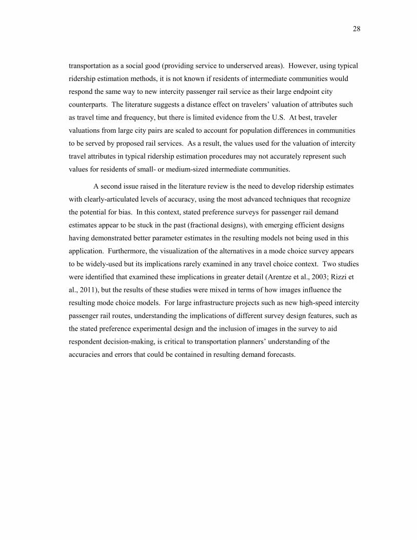
28
transportation as a social good (providing service to underserved areas). However, using typical
ridership estimation methods, it is not known if residents of intermediate communities would
respond the same way to new intercity passenger rail service as their large endpoint city
counterparts. The literature suggests a distance effect on travelers’ valuation of attributes such
as travel time and frequency, but there is limited evidence from the U.S. At best, traveler
valuations from large city pairs are scaled to account for population differences in communities
to be served by proposed rail services. As a result, the values used for the valuation of intercity
travel attributes in typical ridership estimation procedures may not accurately represent such
values for residents of small- or medium-sized intermediate communities.
A second issue raised in the literature review is the need to develop ridership estimates
with clearly-articulated levels of accuracy, using the most advanced techniques that recognize
the potential for bias. In this context, stated preference surveys for passenger rail demand
estimates appear to be stuck in the past (fractional designs), with emerging efficient designs
having demonstrated better parameter estimates in the resulting models not being used in this
application. Furthermore, the visualization of the alternatives in a mode choice survey appears
to be widely-used but its implications rarely examined in any travel choice context. Two studies
were identified that examined these implications in greater detail (Arentze et al., 2003; Rizzi et
al., 2011), but the results of these studies were mixed in terms of how images influence the
resulting mode choice models. For large infrastructure projects such as new high-speed intercity
passenger rail routes, understanding the implications of different survey design features, such as
the stated preference experimental design and the inclusion of images in the survey to aid
respondent decision-making, is critical to transportation planners’ understanding of the
accuracies and errors that could be contained in resulting demand forecasts.
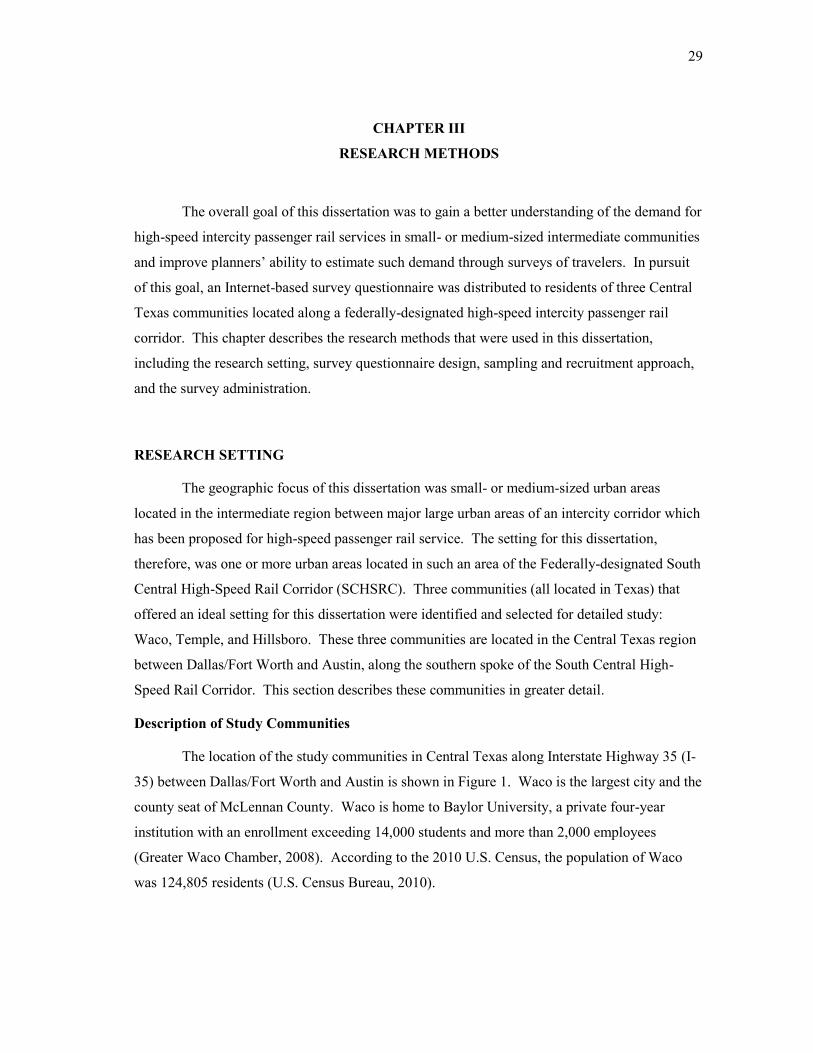
29
CHAPTER III
RESEARCH METHODS
The overall goal of this dissertation was to gain a better understanding of the demand for
high-speed intercity passenger rail services in small- or medium-sized intermediate communities
and improve planners’ ability to estimate such demand through surveys of travelers. In pursuit
of this goal, an Internet-based survey questionnaire was distributed to residents of three Central
Texas communities located along a federally-designated high-speed intercity passenger rail
corridor. This chapter describes the research methods that were used in this dissertation,
including the research setting, survey questionnaire design, sampling and recruitment approach,
and the survey administration.
RESEARCH SETTING
The geographic focus of this dissertation was small- or medium-sized urban areas
located in the intermediate region between major large urban areas of an intercity corridor which
has been proposed for high-speed passenger rail service. The setting for this dissertation,
therefore, was one or more urban areas located in such an area of the Federally-designated South
Central High-Speed Rail Corridor (SCHSRC). Three communities (all located in Texas) that
offered an ideal setting for this dissertation were identified and selected for detailed study:
Waco, Temple, and Hillsboro. These three communities are located in the Central Texas region
between Dallas/Fort Worth and Austin, along the southern spoke of the South Central High-
Speed Rail Corridor. This section describes these communities in greater detail.
Description of Study Communities
The location of the study communities in Central Texas along Interstate Highway 35 (I-
35) between Dallas/Fort Worth and Austin is shown in Figure 1. Waco is the largest city and the
county seat of McLennan County. Waco is home to Baylor University, a private four-year
institution with an enrollment exceeding 14,000 students and more than 2,000 employees
(Greater Waco Chamber, 2008). According to the 2010 U.S. Census, the population of Waco
was 124,805 residents (U.S. Census Bureau, 2010).
30
Figure 1: Location of Study Communities in Central Texas (Sperry and Morgan, 2011)
31
Temple is the largest city in Bell County and is a major regional center for the healthcare
and manufacturing industries. Major employers in Temple include Scott & White Health
Systems (8,000 employees), the Central Texas Veterans Health Care System (2,269), and
McLane Distribution Company (2,255) (Temple Economic Development Corporation, 2010).
According to the 2010 U.S. Census, the population of Temple was 66,102 residents (U.S. Census
Bureau, 2010). Hillsboro is the largest city and county seat of Hill County and is located just
south of where I-35 divides into two auxiliary routes (I-35E and I-35W). According to the 2010
U.S. Census, the population of Hillsboro was 8,456 residents (U.S. Census Bureau, 2010).
The heavily-traveled Interstate 35 highway corridor passes through each of the three
study communities on its path between Dallas/Fort Worth and Austin. In 2010, the annual
average daily traffic (AADT) along this section of I-35 was approximately 55,000 vehicles per
day (Texas Department of Transportation, 2010). In addition to automobile travel, intercity
transportation alternatives in the study communities included intercity bus, conventional Amtrak
intercity passenger rail service, and regional connecting airline service. Intercity bus service by
Greyhound Lines and others served Waco with between 5 and 9 daily trips in each direction on a
basic route along I-35 (Greyhound Lines, 2011). Amtrak’s Texas Eagle long-distance train
made one daily stop in both directions in Temple, McGregor (20 miles southwest of Waco), and
Cleburne (30 miles northwest of Hillsboro). Travel time from Temple to Fort Worth on the
Texas Eagle was approximately 2.5 hours (National Railroad Passenger Corporation, 2011). In
the 12-month period ending September 2010, passenger activity at the three Texas Eagle stations
in or near the study communities was as follows: Temple, 15,426 passengers; McGregor, 4,240
passengers; and Cleburne, 3,130 passengers (Amtrak Government Affairs, 2010). Regional
airline service was available in Waco (Waco Regional Airport/ACT) and Temple (via nearby
Killeen-Fort Hood Regional Airport/GRK), connecting those communities to airline hubs at
Dallas/Fort Worth (Dallas-Fort Worth International/DFW) and Houston (Houston George Bush
Intercontinental Airport/IAH) with between 3 and 10 flights daily.
Intercity Passenger Rail Development in Study Communities
Although the region was served by the Amtrak Texas Eagle passenger rail route, the
large population and economic significance of the area (often called the Texas Triangle, formed
by linking Dallas-Fort Worth, San Antonio, and Houston) has resulted in a number of proposed
high-speed or higher-speed intercity passenger rail initiatives for the region. In 1990, the Texas
32
Legislature established the Texas High-Speed Rail Authority (THSRA), which solicited
franchise applications from two consortiums (named the Texas FasTrac and the Texas TGV) to
establish high-speed passenger rail service through the region. While a franchise was awarded to
the Texas TGV consortium, the project was ultimately canceled in 1994. A more detailed
account of the THSRA and its short history can be found in Roco and Olson (2004). While many
of the details of the failed venture are not important for this dissertation, it is worth noting the
initiative was primarily conceived to improve intercity mobility between the three corners of the
Texas Triangle (Dallas/Fort Worth, San Antonio and Houston) and including the state capital of
Austin. The Texas TGV franchise did not include any intermediate stops between the
aforementioned urban areas in its original proposal (Texas TGV, 1991). It is noted, however, that
the other potential franchise, the Texas FasTrac, did include stops in Waco and Bryan/College
Station in its proposal (Texas FasTrac, 1991), and that the successful Texas TGV franchise later
included these cities in its “Corporation Preferred” alternative (Charles River Associates, 1993).
After the cancellation of the Texas TGV and the abolishment of the Texas High-Speed
Rail Authority, momentum for the creation of improved passenger rail service along the I-35
corridor continued, resulting in the designation of the SCHSRC in 2000. The Federal high-speed
rail corridors program was established in the Intermodal Surface Transportation Efficiency Act
(ISTEA) in 1991 (Federal Railroad Administration, 2009a). The original objective of the
program was to provide funding for highway-rail grade crossing improvements along major
intercity corridors nationwide. To date, eleven unique corridors have been designated as a part
of this program (Federal Railroad Administration, 2011a). The SCHSRC was designated
pursuant to Section 1103(c) of the Transportation Equity Act for the 21st Century (TEA-21), and
directed the corridor to link Dallas/Fort Worth with Austin and San Antonio, Texas (Federal
Railroad Administration, 2009b). With Dallas/Fort Worth as a hub, the SCHSRC also includes
spokes from Dallas/Fort Worth north to Oklahoma City and Tulsa in Oklahoma, and east to
Texarkana and Little Rock in Arkansas. Since 2000, more than $2.558 million has been
allocated for grade crossing improvements in the three states – Arkansas, Oklahoma, and Texas.
In spite of these investments, however, intercity passenger rail service along the corridor has not
changed substantially in the last decade. It is noted that the official designation of the SCHSRC
does not specifically mention any intermediate communities between Dallas/Fort Worth, Austin,
and San Antonio in its language, and that the exact routing of new high-speed intercity passenger
rail services between these communities remains unknown, left to the direction of future

33
ridership or environmental studies. As a result, while the statutory corridor definition does not
necessarily limit the feasibility of new intercity passenger rail services being routed to
conveniently serve intermediate communities, any efforts to serve intermediate communities
would go beyond the statutory definition for the corridor. This may be challenging, particularly
if serving intermediate communities was feasible only with significantly-higher investment.
Recent interest in high-speed intercity passenger rail service (Federal Railroad
Administration, 2009a; Peterman et al., 2009) has revived interest in developing new high-speed
passenger rail services along the Interstate 35 corridor. In October 2010, the Texas Department
of Transportation (TxDOT) was awarded an Federal Railroad Administration (FRA) grant of
$5.6 million to create feasibility studies, a service development plan, and environmental
documentation for new rail service along the entire I-35 corridor from Oklahoma City to the
Mexican border in Laredo (Amtrak Government Affairs, 2010; Federal Railroad Administration,
2010; Wear, 2010). In its regular meeting on December 16, 2010, the Texas Transportation
Commission (2010) authorized the use of the FRA grant for those purposes, and U.S.
Department of Transportation Secretary Ray LaHood officially announced the award on
November 18, 2011 (Federal Railroad Administration, 2011b). One alternative plan proposed
for high-speed rail service in the Texas Triangle which includes provisions for service to
intermediate communities is the “Texas T-Bone” plan put forth by a local government
corporation called the South Central High-Speed Rail and Transportation Authority, Inc.
(SCHSRTA) and a group of local government officials and affiliated city, county, educational,
and private entities known as the Texas High Speed Rail and Transportation Corporation
(THSRTC). The “Texas T-Bone” corridor would connect the major communities along I-35
with new service, and connect Houston to this corridor with a link in Temple via Bryan/College
Station. At of this writing, however, the status of the “Texas T-Bone” project and the plans of
the SCHSRTA to implement its vision remain unknown.
The setting for this dissertation was three communities in Central Texas: Waco, Temple,
and Hillsboro. These three communities were the ideal setting for this research because they are
all located along the Federally-designated South Central High-Speed Rail Corridor in the
intermediate area between Dallas/Fort Worth and Austin, Texas. Although the region was
served by intercity passenger rail service at the time of the study (the Amtrak Texas Eagle long-
distance train), the area has long been considered for improved high-speed intercity passenger

34
rail service. However, previous efforts to establish high-speed passenger rail in the region (in
the early 1990s) did not include these intermediate areas in initial plans. As a result, no detailed
studies on the potential demand or valuation of intercity passenger rail service in these
communities exist. Furthermore, it is unclear the extent to which recent developments, most
notably the $5.6 million FRA grant awarded to TxDOT in 2011 to study high-speed passenger
rail service along I-35 from Oklahoma City to Laredo, will attempt to assess the demand for
intercity rail transportation to these intermediate communities. Consequently, due to the
geographic location of the communities and the previous and current attempts to establish high-
speed intercity passenger rail in the communities, the three communities selected for more
detailed examination in this dissertation offer an ideal setting for a study of this nature.
SURVEY QUESTIONNAIRE
Questionnaire Design
To obtain data to answer the research questions examined in this dissertation, an
Internet-based survey questionnaire was distributed to residents of three Central Texas
communities: Waco, Temple, and Hillsboro. The survey, titled the Central Texas Passenger
Rail Survey, was conducted using a website on the Internet and contained 19 survey questions
across 11 unique website pages. A website domain name with a locally-identifiable sub-domain
(http://www.railsurvey.org/centex) was obtained to host the survey questionnaire. The open-
source Internet survey software application LimeSurvey® was installed on the domain and used
to publish the survey questions onto the website (LimeSurvey, 2010).
The first page of the survey contained a short message to the participant explaining the
purpose of the survey, a notice about the rights of the research participant, and contact
information. Next, the respondent identified his or her home community. The respondent was
then asked about his or her recent intercity travel history between their home community and
five large urban areas in Texas: Austin, Dallas, Fort Worth, Houston, and San Antonio.
Respondents were asked to indicate the number of automobile trips to these urban areas during
the last six months, separated by trips for business purposes and trips for personal or non-
business purposes. These questions were included to better-understand the market for intercity
automobile travel among residents of the study communities.
35
Next, the respondents were presented with a description of a proposed intercity
passenger rail service in their community and a hypothetical scenario consisting of a personal or
non-business related trip between his or her home community and central Dallas. For selected
respondents, this description was supplemented with an image of the exterior and interior of a
passenger train. Given this scenario, the respondent was presented with six stated preference
questions asking him or her to select between automobile or intercity train for this hypothetical
trip. These two aspects of the survey design (stated preference experimental design and
visualization of travel alternatives) are discussed in greater detail in subsequent sections.
After the six stated preference questions, the respondent was asked about his or her
experience with a various rail transportation modes ranging from urban rail transit service in
Texas to intercity passenger rail in the U.S. and high-speed intercity passenger rail in Europe or
Asia. Respondents were asked to rate their level of experience with each rail mode on a four-
point scale. The respondent was then asked about his or her potential use of new intercity
passenger rail service in their community as well as their opinion of certain aspects of travel via
intercity passenger rail relative to automobile travel. A seven-point Likert scale ranging from
“Strongly Disagree” to “Strongly Agree” was utilized for these questions. The respondent was
then asked about his or her opinion on the potential impacts of new intercity passenger rail
service in their home community on various aspects of the quality of life, business and
employment, and tourism in their community. These questions used the same seven-point Likert
scale as the prior question set. The survey concluded with a section containing questions about
the respondent’s demographic characteristics and also provided a space for the respondent to
provide comments about the survey or the potential for passenger rail development in his or her
community. A copy of the survey questionnaire can be found in Appendix A.
Institutional Review Board Approval
Since this dissertation involved interaction with human subjects, approval from the
Texas A&M University Office of Research Compliance’s Institutional Review Board (IRB) was
required before undertaking data collection. An initial application was submitted to the IRB on
March 16, 2011. The IRB protocol (#2011-0194) was ruled “exempt from IRB review” and
approved on March 29, 2011. Further revisions to the survey questionnaire were necessary to
reduce the number of questions and enhance the layout, readability, and overall comprehension
of the survey questions. Consequently, an amendment was submitted to the IRB on April 19,
36
2011 requesting approval of the revised version of the survey questionnaire. The IRB approved
the amendment request on May 3, 2011. Appendix B contains documentation of IRB approval
for the initial protocol and amendment.
STATED PREFERENCE QUESTION DESIGN
The purpose of this dissertation was to gain a better understanding of the demand for
high-speed intercity passenger rail services in small- or medium-sized intermediate communities
and improve planners’ ability to estimate such demand through surveys of travelers. One
alternative which can be used to support intercity mobility in such communities is some form of
passenger rail. However, in corridors where passenger rail is not yet available as an alternative,
an important tool that planners have for studying the effects of such modes is a stated preference
survey. The second part of the Internet survey used in this dissertation was a six-question stated
preference exercise designed to identify how travelers in the study communities value their
options for intercity travel. This section describes the design of the stated preference questions.
Basic Design Information
The stated preference questions contained exercises where the respondent was asked to
consider a choice between automobile and proposed intercity passenger rail service for a
hypothetical trip between his or her home community and the central business district of Dallas,
Texas. Even though it was a viable alternative surface intercity travel mode, intercity bus was
not included as a travel alternative in this dissertation because the focus was on how residents of
a community valued proposed intercity passenger rail service. Commercial airline was also not
included as an alternative because the focus of this dissertation was on how passenger rail could
support mobility for the intermediate communities of an intercity corridor, whereas most airline
trips in this context are primarily regional airlines connecting to long-haul flights. While it
would have been preferable for the respondent to consider an actual trip recently made by him or
her from their home community to Dallas in these exercises, it was not practical to do so given
that the dissertation was targeting all community residents and not necessarily recent or frequent
intercity travelers. Furthermore, using a hypothetical trip for the stated preference exercise
decreased the inherent variability in the survey attributed to different types of intercity trips and
destinations that might be found among respondents.
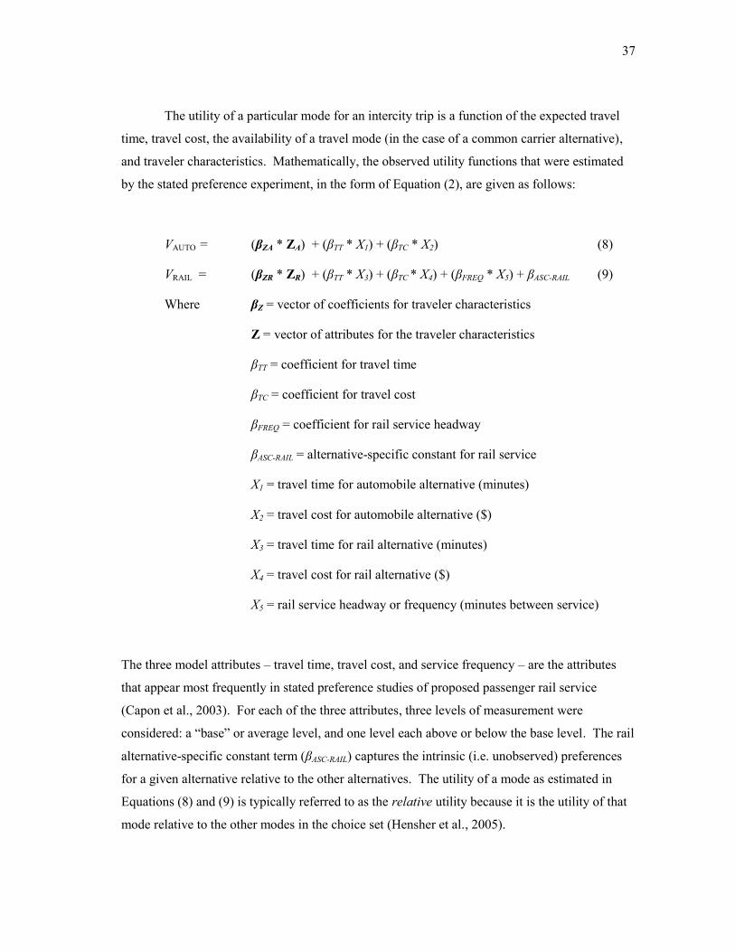
37
The utility of a particular mode for an intercity trip is a function of the expected travel
time, travel cost, the availability of a travel mode (in the case of a common carrier alternative),
and traveler characteristics. Mathematically, the observed utility functions that were estimated
by the stated preference experiment, in the form of Equation (2), are given as follows:
VAUTO = (βZA * ZA) + (βTT * X1) + (βTC * X2) (8)
VRAIL = (βZR * ZR) + (βTT * X3) + (βTC * X4) + (βFREQ * X5) + βASC-RAIL (9)
Where βZ = vector of coefficients for traveler characteristics
Z = vector of attributes for the traveler characteristics
βTT = coefficient for travel time
βTC = coefficient for travel cost
βFREQ = coefficient for rail service headway
βASC-RAIL = alternative-specific constant for rail service
X1 = travel time for automobile alternative (minutes)
X2 = travel cost for automobile alternative ($)
X3 = travel time for rail alternative (minutes)
X4 = travel cost for rail alternative ($)
X5 = rail service headway or frequency (minutes between service)
The three model attributes – travel time, travel cost, and service frequency – are the attributes
that appear most frequently in stated preference studies of proposed passenger rail service
(Capon et al., 2003). For each of the three attributes, three levels of measurement were
considered: a “base” or average level, and one level each above or below the base level. The rail
alternative-specific constant term (βASC-RAIL) captures the intrinsic (i.e. unobserved) preferences
for a given alternative relative to the other alternatives. The utility of a mode as estimated in
Equations (8) and (9) is typically referred to as the relative utility because it is the utility of that
mode relative to the other modes in the choice set (Hensher et al., 2005).
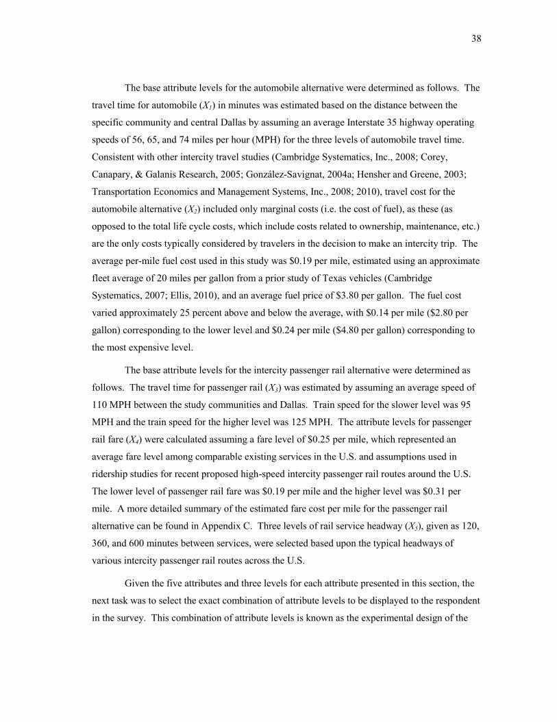
38
The base attribute levels for the automobile alternative were determined as follows. The
travel time for automobile (X1) in minutes was estimated based on the distance between the
specific community and central Dallas by assuming an average Interstate 35 highway operating
speeds of 56, 65, and 74 miles per hour (MPH) for the three levels of automobile travel time.
Consistent with other intercity travel studies (Cambridge Systematics, Inc., 2008; Corey,
Canapary, & Galanis Research, 2005; González-Savignat, 2004a; Hensher and Greene, 2003;
Transportation Economics and Management Systems, Inc., 2008; 2010), travel cost for the
automobile alternative (X2) included only marginal costs (i.e. the cost of fuel), as these (as
opposed to the total life cycle costs, which include costs related to ownership, maintenance, etc.)
are the only costs typically considered by travelers in the decision to make an intercity trip. The
average per-mile fuel cost used in this study was $0.19 per mile, estimated using an approximate
fleet average of 20 miles per gallon from a prior study of Texas vehicles (Cambridge
Systematics, 2007; Ellis, 2010), and an average fuel price of $3.80 per gallon. The fuel cost
varied approximately 25 percent above and below the average, with $0.14 per mile ($2.80 per
gallon) corresponding to the lower level and $0.24 per mile ($4.80 per gallon) corresponding to
the most expensive level.
The base attribute levels for the intercity passenger rail alternative were determined as
follows. The travel time for passenger rail (X3) was estimated by assuming an average speed of
110 MPH between the study communities and Dallas. Train speed for the slower level was 95
MPH and the train speed for the higher level was 125 MPH. The attribute levels for passenger
rail fare (X4) were calculated assuming a fare level of $0.25 per mile, which represented an
average fare level among comparable existing services in the U.S. and assumptions used in
ridership studies for recent proposed high-speed intercity passenger rail routes around the U.S.
The lower level of passenger rail fare was $0.19 per mile and the higher level was $0.31 per
mile. A more detailed summary of the estimated fare cost per mile for the passenger rail
alternative can be found in Appendix C. Three levels of rail service headway (X5), given as 120,
360, and 600 minutes between services, were selected based upon the typical headways of
various intercity passenger rail routes across the U.S.
Given the five attributes and three levels for each attribute presented in this section, the
next task was to select the exact combination of attribute levels to be displayed to the respondent
in the survey. This combination of attribute levels is known as the experimental design of the
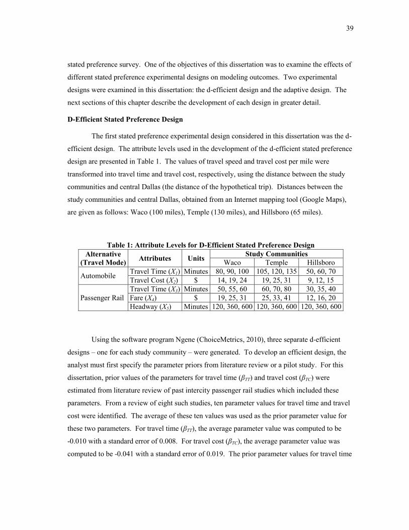
39
stated preference survey. One of the objectives of this dissertation was to examine the effects of
different stated preference experimental designs on modeling outcomes. Two experimental
designs were examined in this dissertation: the d-efficient design and the adaptive design. The
next sections of this chapter describe the development of each design in greater detail.
D-Efficient Stated Preference Design
The first stated preference experimental design considered in this dissertation was the d-
efficient design. The attribute levels used in the development of the d-efficient stated preference
design are presented in Table 1. The values of travel speed and travel cost per mile were
transformed into travel time and travel cost, respectively, using the distance between the study
communities and central Dallas (the distance of the hypothetical trip). Distances between the
study communities and central Dallas, obtained from an Internet mapping tool (Google Maps),
are given as follows: Waco (100 miles), Temple (130 miles), and Hillsboro (65 miles).
Table 1: Attribute Levels for D-Efficient Stated Preference Design
Alternative
(Travel Mode) Attributes Units
Study Communities
Waco Temple Hillsboro
Automobile Travel Time (X1) Minutes 80, 90, 100 105, 120, 135 50, 60, 70
Travel Cost (X2) $ 14, 19, 24 19, 25, 31 9, 12, 15
Passenger Rail
Travel Time (X3) Minutes 50, 55, 60 60, 70, 80 30, 35, 40
Fare (X4) $ 19, 25, 31 25, 33, 41 12, 16, 20
Headway (X5) Minutes 120, 360, 600 120, 360, 600 120, 360, 600
Using the software program Ngene (ChoiceMetrics, 2010), three separate d-efficient
designs – one for each study community – were generated. To develop an efficient design, the
analyst must first specify the parameter priors from literature review or a pilot study. For this
dissertation, prior values of the parameters for travel time (βTT) and travel cost (βTC) were
estimated from literature review of past intercity passenger rail studies which included these
parameters. From a review of eight such studies, ten parameter values for travel time and travel
cost were identified. The average of these ten values was used as the prior parameter value for
these two parameters. For travel time (βTT), the average parameter value was computed to be
-0.010 with a standard error of 0.008. For travel cost (βTC), the average parameter value was
computed to be -0.041 with a standard error of 0.019. The prior parameter values for travel time

40
and travel cost were reasonable, containing the proper sign and a value of time of $14.83 per
hour. For the remaining two parameters, rail service frequency/headway and the rail alternative-
specific constant, only two prior values could be identified from the literature. The average
parameter value for rail service frequency or headway (βFREQ) was -0.0025 and used with no
standard error. The alternative-specific constant was assumed to be zero with a standard error of
0.5. This was a conservative approach, recognizing that there will likely be an alternative-
specific constant of some magnitude but unknown direction. The Ngene software was
programmed to search for a D-efficient design using 18 rows blocked into six blocks of three
choice situations per block. Three separate D-efficient designs were created, one for each of the
three study communities. The estimated D-errors for each of the designs were 0.000383 for
Waco, 0.000221 for Temple, and 0.000503 for Hillsboro – all acceptable errors for a preliminary
design. Details of the development of the D-efficient design can be found in Appendix D (prior
parameters estimates) and Appendix E (Ngene syntax and output).
Adaptive Stated Preference Design
The second stated preference design considered in this dissertation was a non-
experimental adaptive design which adjusted the attribute levels presented to the respondent
based on the respondent’s previous selections. The adaptive design was implemented as follows.
In the first question, values for travel speed, travel cost per mile, and rail service headway were
randomly-selected from anywhere within the range of attribute levels given under the “Question
1” column in Table 2, including the endpoints. The selected values for speed and cost were then
transformed by the distance between the respondent’s home community and central Dallas and
presented to the respondent in terms of total travel time and total travel cost.
Table 2: Endpoints of Range of Attribute Levels for Adaptive Design
Alternative
(Travel Mode) Attributes Units
Stated Preference Question
Question 1 Question 2 Question 3
Automobile Travel Time (X1) Miles/Hour (60,69) (56,73) (55,74)
Travel Cost (X2) $/Mile (0.17,0.20) (0.14,0.23) (0.12,0.25)
Passenger Rail
Travel Time (X3) Miles/Hour (100,119) (95,124) (90,129)
Fare (X4) $/Mile (0.21,0.28) (0.19,0.30) (0.17,0.32)
Headway (X5) Hours (4,7) (2,9) (1,10)

41
In the second adaptive stated preference question, attribute levels were randomly-
generated in a similar fashion, except that the range from which the values were selected was
wider than in the first question. Furthermore, the selection of attribute levels was constrained
such that the travel time and travel cost (and headway for rail) of the alternative chosen in the
first question increased while the travel time, travel cost, and headway of the alternative not
chosen decreased. For example, if a respondent selected automobile in the first question, the
second question lowered the cost of the passenger rail service and increased the cost of the
automobile. Thus, the attribute levels presented in the second question were “adapted” based on
the response provided in the first question. Selection of attribute levels for the third question
was performed in a similar manner, adjusting the attribute levels displayed in the third question
based upon the selected alternative in the second question.
A total of six stated preference questions were presented to each respondent, a
randomly-selected block of three questions from the d-efficient design and three questions
generated using the adaptive design. The questions were presented across three website pages
with each page containing two questions, one of each design type. This was possible in part
because the technology associated with the Internet-based survey mode allowed for the requisite
coding and scripting to allow for questions drawn from both experimental designs to be
presented. This approach was a benefit to the overall research as it allowed for the two
experimental designs to be compared without having to develop two separate versions of the
survey questionnaire and having to account for the potential demographic differences in the
respondents viewing each. A screen shot of a typical stated preference question set used in this
survey is given in Figure 2.

42
Figure 2: Screen Shot of Typical Stated Preference Question Set
VISUALIZATION
Literature on the design of stated preference experiments has suggested the use of visual
material to support text descriptions of alternatives or attributes in the exercise. The motivation
for adding photos or other graphics to the stated preference exercise is that such material might
aid the respondent’s decision-making process by making the choices more tangible to the
respondent. In the case of alternatives that do not yet exist (such as new intercity passenger rail),
visual aids may also be used to “introduce” the respondent to the hypothetical alternative. In this
context, it has been suggested that visual material could be used to portray the new rail mode as
“flashy” and overstress its attractive features – effectively distracting the respondent from
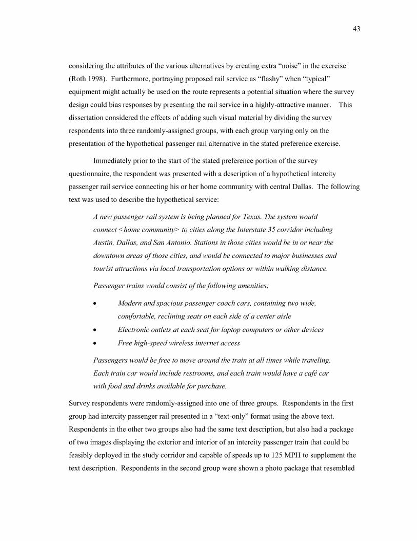
43
considering the attributes of the various alternatives by creating extra “noise” in the exercise
(Roth 1998). Furthermore, portraying proposed rail service as “flashy” when “typical”
equipment might actually be used on the route represents a potential situation where the survey
design could bias responses by presenting the rail service in a highly-attractive manner. This
dissertation considered the effects of adding such visual material by dividing the survey
respondents into three randomly-assigned groups, with each group varying only on the
presentation of the hypothetical passenger rail alternative in the stated preference exercise.
Immediately prior to the start of the stated preference portion of the survey
questionnaire, the respondent was presented with a description of a hypothetical intercity
passenger rail service connecting his or her home community with central Dallas. The following
text was used to describe the hypothetical service:
A new passenger rail system is being planned for Texas. The system would
connect <home community> to cities along the Interstate 35 corridor including
Austin, Dallas, and San Antonio. Stations in those cities would be in or near the
downtown areas of those cities, and would be connected to major businesses and
tourist attractions via local transportation options or within walking distance.
Passenger trains would consist of the following amenities:
Modern and spacious passenger coach cars, containing two wide,
comfortable, reclining seats on each side of a center aisle
Electronic outlets at each seat for laptop computers or other devices
Free high-speed wireless internet access
Passengers would be free to move around the train at all times while traveling.
Each train car would include restrooms, and each train would have a café car
with food and drinks available for purchase.
Survey respondents were randomly-assigned into one of three groups. Respondents in the first
group had intercity passenger rail presented in a “text-only” format using the above text.
Respondents in the other two groups also had the same text description, but also had a package
of two images displaying the exterior and interior of an intercity passenger train that could be
feasibly deployed in the study corridor and capable of speeds up to 125 MPH to supplement the
text description. Respondents in the second group were shown a photo package that resembled
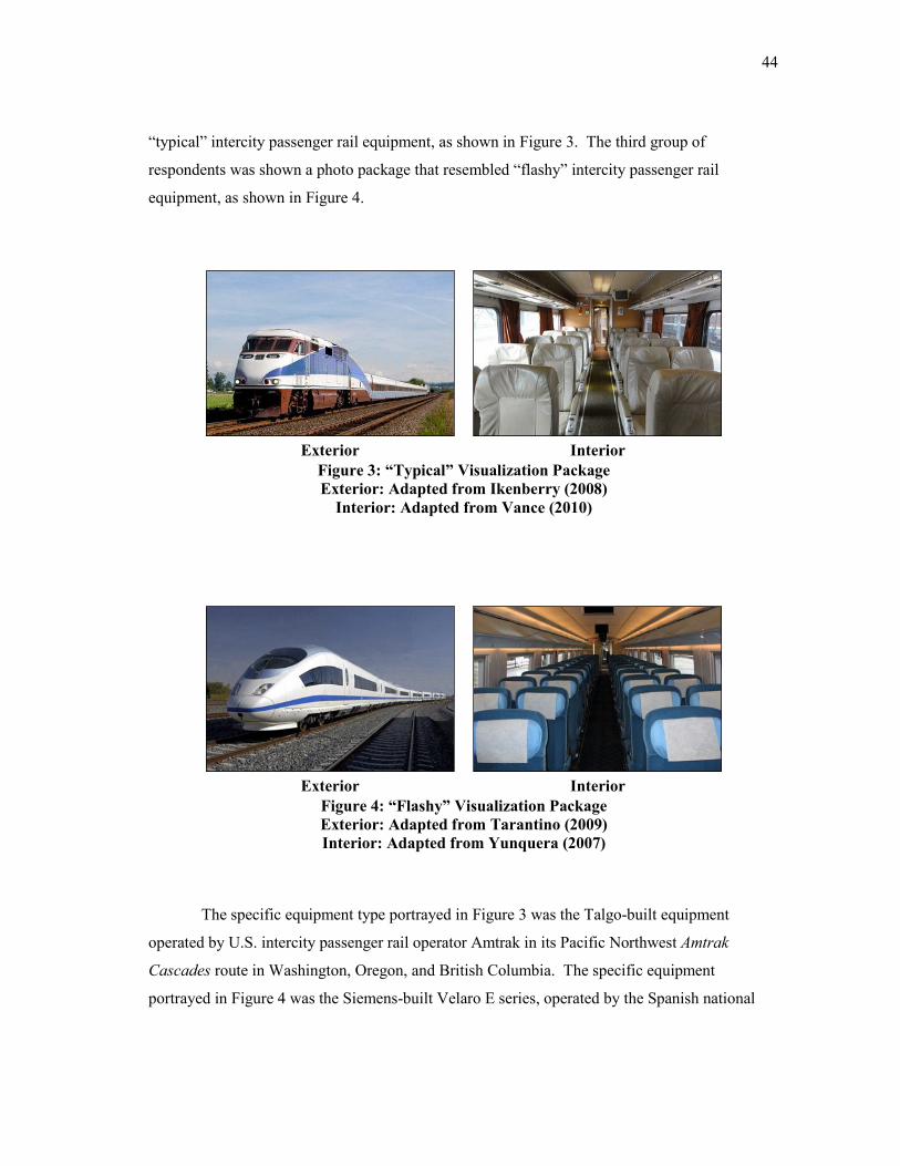
44
“typical” intercity passenger rail equipment, as shown in Figure 3. The third group of
respondents was shown a photo package that resembled “flashy” intercity passenger rail
equipment, as shown in Figure 4.
Exterior Interior
Figure 3: “Typical” Visualization Package
Exterior: Adapted from Ikenberry (2008)
Interior: Adapted from Vance (2010)
Exterior Interior
Figure 4: “Flashy” Visualization Package
Exterior: Adapted from Tarantino (2009)
Interior: Adapted from Yunquera (2007)
The specific equipment type portrayed in Figure 3 was the Talgo-built equipment
operated by U.S. intercity passenger rail operator Amtrak in its Pacific Northwest Amtrak
Cascades route in Washington, Oregon, and British Columbia. The specific equipment
portrayed in Figure 4 was the Siemens-built Velaro E series, operated by the Spanish national

45
railroad Renfé as the AVE S103 series on various routes in Spain. As of this writing, it was one
of the fastest trains in commercial operation in the world. The photos were edited prior to their
use in the survey to ensure as much consistency between the two photo packages, reducing the
potential for variation caused by inconsistencies in the color of the equipment, interior lighting,
and background and foreground elements. The combined text and image description of the
hypothetical intercity passenger rail service on the ‘Travel Choices Introduction” page of the
survey questionnaire is shown in Figure 5.
Figure 5: Screen Shot of Travel Choices Introduction Screen
SAMPLE SIZE
The minimum required sample size for typical transportation surveys can be computed
using equations that are well-established in the statistics literature. However, as Bliemer and

46
Rose (2005) point out, two common sampling approaches (simple random sampling and
exogenous stratified random sampling) are not appropriate for stated preference surveys because
each requires an a priori knowledge of the choice proportions. This is particularly an issue if a
hypothetical alternative is being considered in the stated preference survey, and as such, the
analyst may have no working knowledge of the proportion of the market that might opt for such
alternative. Bliemer and Rose (2005) have suggested that the minimum required sample size (N)
for efficient stated preference experiments can be computed using Equation (10) for each
parameter to be estimated by incorporating the prior parameters data that are used to develop the
initial d-efficient design.
2 2
2ˆk k
k
k
tN
(10)
Where βk = prior parameter estimate for attribute k
σβk = standard error of the prior parameter estimate βk
t = asymptotic t-ratio for desired level of significance α
Using the estimated β and σ reported previously and a t-ratio of 1.96 (α=0.05), Equation (10)
estimates that three respondents were required for a significant sample size on the travel time
parameter while a single respondent was required for the travel cost parameter. No such
estimate was computed for the rail service headway parameter as a sample of parameter priors
could not be obtained that was sufficiently large enough to estimate a standard error.
The Ngene software program estimates a minimum sample size using a metric called the
Sp-error, which is defined as the number of times a particular stated preference experimental
design would need to be replicated to achieve a statistically-significant t-ratio (t=1.96, α=0.05)
for each of the model parameters, given the parameter priors assumed (ChoiceMetrics, 2010).
An Sp-error value is estimated for each model parameter and the largest such value represents
the minimum required number of replications (i.e. minimum sample size) for the design. From
the Ngene output (Appendix E), the minimum sample sizes desired from each study community
were estimated to be: Waco, 83 responses; Temple, 27 responses; and Hillsboro, 72 responses.
As an alternative to the minimum sample size suggested by Bliemer and Rose (2005) or
estimated by the Ngene output, a number of “rules of thumb” are available for estimating a
47
minimum sample size for stated preference surveys. One such rule, outlined by Orme (2010),
uses the following Equation (11):
SJ
lN
*500 (11)
Where l* = maximum number of levels taken by any single attribute
J = number of alternatives considered in stated preference question
S = number of choice tasks considered by each respondent
For this dissertation, at the given values for l* (3), J (2), and S (3), the minimum sample size as
defined by Equation (11) was 250 respondents. It is noted that although the respondent actually
considered six choice tasks on a single survey (three each of two different experimental designs,
S was set equal to 3 for the purposes of Equation (11) to ensure that the minimum required
sample size would be sufficient for separate analysis of data from each stated preference
experimental design. Practical guidelines from the same reference (Orme, 2010) suggest that for
segmentation studies (such as the one in this dissertation), a minimum of 200 respondents per
segment is ideal. As such, a minimum of 250 respondents was the goal for each version of the
survey (each of three visualization packages), for a desired minimum total of 750 respondents
with sufficiently-completed stated preference exercises.
SURVEY ADMINISTRATION
The survey questionnaire was administered to a convenience sample of residents in the
three study communities via the Internet. The use of the Internet was justified in this survey
because it allowed for respondents to be randomly-assigned to one of the three visualization
packages and one of the six blocks of d-efficient stated preference questions. Additionally, the
Internet allowed for the script used in the adaptive stated preference survey questions to be
executed in a timely fashion that would otherwise be impractical with other survey medium.
A convenience sample was necessary because a suitable sampling frame (such as a
comprehensive list of valid e-mail addresses of community residents) could not be identified.
Therefore, the following four approaches were used to recruit residents of the study communities
to the survey questionnaire:

48
Invitation to participate in the survey distributed across the e-mail distribution lists of
organizations in the study communities;
News articles published in local newspapers or contained within weekly e-mail
newsletters of community groups in the study communities;
Purchased newspaper advertisements in local newspapers in the study communities; and
On-site recruitment of potential subjects at selected locations in the study communities.
Major employers and organizations in the three study communities were contacted to request
permission to distribute an approved recruitment message across its e-mail distribution list. The
recruitment e-mail message contained a short description of the study and a link to the survey
website. Recruitment e-mail messages were sent to municipal employees as well as employees
of the local school districts in each of the three study communities. Other e-mail distribution
lists that received the recruitment e-mail message included various local resident organizations
and business groups. News articles promoting the survey were included in the weekly e-mail
newsletters published by the Waco and Temple Chambers of Commerce, and news articles about
the survey appeared in the Temple Daily Telegram newspaper on June 9 and July 7, 2011. Print
advertisements recruiting community residents to participate in the survey were purchased in
local newspapers in each of the three study communities. Recruitment advertisements were
published in the Waco Tribune and the Temple Daily Telegram on July 9-11 and 13-14, 2011
and in the Hillsboro Reporter on July 11 and 14, 2011.
To supplement these recruitment efforts, field visits were made to each of the study
communities to directly recruit subjects to participate in the survey and to provide community
residents who might not have access to a computer with Internet capabilities the opportunity to
participate in the survey. On June 30, 2011, postcards containing the survey website were
distributed to employees of the Outlets at Hillsboro, a major employer in Hillsboro. Additionally,
postcards were left in the reception area of a local social services office and the Hillsboro Public
Library. On August 2, 2011, researchers visited Waco and Temple to outreach to residents of
those communities. Temple Public Library patrons were recruited during the mid-day period to
participate in the survey. A study room area at the library was equipped with laptop computers
to facilitate this effort. That evening, attendees of a “National Night Out” neighborhood event in
Waco were recruited to participate in the survey via laptops set up in an adjacent community
center. Residents participating in the survey during the field visits viewed the same survey as
49
respondents who participated in the survey via other recruitment efforts, and researchers assisted
respondents with questions about how to take the survey or questions about operating of the
computer equipment. All recruitment materials used in this study were approved by the Texas
A&M University IRB and can be found in Appendix F.
The Internet survey questionnaire was open and accessible to receive responses starting
on May 4, 2011 and ending on August 2, 2011 -- a total of 91 days of survey data collection.
During this time period, a total of 1,270 residents from the three study communities visited the
website to take the survey from which 1,160 (91.3 percent) valid and completed surveys were
obtained. Given the number of questions on the survey, a break-off or incompletion rate of less
than 10 percent was acceptable. The number of surveys completed from each community was as
follows: Waco, 591 surveys (51.0 percent); Temple, 483 surveys (41.6 percent); and Hillsboro,
86 surveys (7.4 percent).
Due to the recruitment methods used, an accurate estimate of the response rate to the
Internet survey could not be estimated. However, to improve the overall participation in the
survey, three Visa gift cards valued at $250 each were offered to three randomly-selected study
participants once the survey period was complete. Upon completion of the survey questionnaire,
participants were provided with a link to a separate Internet survey for the entry into the gift card
drawing. Entry into this drawing was optional and the information collected included the
respondent’s name and telephone number. Collecting the information for the gift card drawing
as a separate survey allowed the respondent’s identities to remain separate from their responses
to the survey questionnaire. A total of 1,020 participants in the survey entered into the drawing
for the gift card. While no formal analyses were conducted on the effectiveness of the gift card
drawing in recruiting residents from the three study communities to the survey questionnaire, it
is noted that more than 88 percent of participants that completed the survey also entered the gift
card drawing. This high number suggested that the opportunity to win one of the gift cards was
well-received among the participants. On August 3, 2011, three respondent names were
randomly-selected from the list of entries into the gift card drawing and a $250 Visa gift card
was mailed to each of the three selected individuals.

50
CHAPTER IV
PRELIMINARY ANALYSIS
The overall goal of this dissertation was to gain a better understanding of the demand for
high-speed intercity passenger rail services in small- or medium-sized intermediate communities
and improve planners’ ability to estimate such demand through the use of stated preference
exercises in traveler surveys. Chapter III described the study setting and survey questionnaire
used to obtain 1,160 survey responses from residents in three Central Texas communities in
pursuit of this goal. A preliminary analysis of the data obtained from the survey questionnaire is
described in this chapter. First, a description of the characteristics of the survey sample is
provided. Second, possible bias resulting from the use of the Internet for this survey is examined
and the need to apply weights to the sample data to account for such bias is determined. Next,
the two stated preference experimental designs examined in this dissertation are evaluated for
non-trading and lexicographic behavior, a set of metrics relating the quality of stated preference
responses. The chapter concludes by examining the effects of visualization of a hypothetical
travel alternative (in this case, passenger rail) on survey behavior and responses.
SAMPLE DESCRIPTION
A total of 1,160 completed surveys were obtained from residents of the three study
communities. The number of surveys completed from each community was as follows: Waco,
591 surveys; Temple, 483 surveys; and Hillsboro, 86 surveys. The number of completed surveys
from Hillsboro was deemed to be insufficient for carrying out this research and thus the 86
surveys obtained from that community were not used in this analysis. Thus, the remainder of
this dissertation will focus exclusively on the data obtained from residents of Waco and Temple.
Details of the demographic and selected travel behavior characteristics of the survey
sample are given in Table 3. In both Waco and Temple, more than 60 percent of the survey
respondents were female. More than half of respondents from both communities reported being
between 45 and 64 years old. The average number of household vehicles, average number of
adults in the respondent’s household, and the average number of children in the respondent’s
household were also consistent between the two communities. On the whole, the sample was
well-educated, with approximately two-thirds of respondents in both communities possessing a
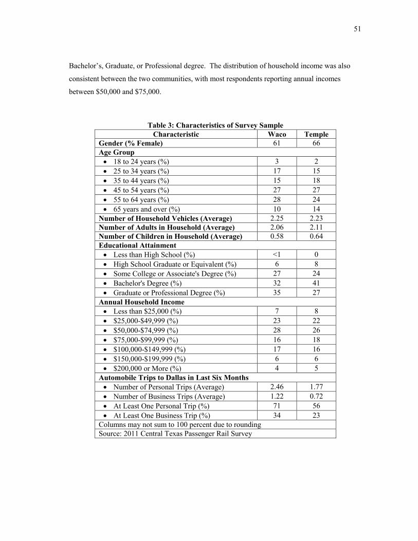
51
Bachelor’s, Graduate, or Professional degree. The distribution of household income was also
consistent between the two communities, with most respondents reporting annual incomes
between $50,000 and $75,000.
Table 3: Characteristics of Survey Sample
Characteristic Waco Temple
Gender (% Female) 61 66
Age Group
18 to 24 years (%) 3 2
25 to 34 years (%) 17 15
35 to 44 years (%) 15 18
45 to 54 years (%) 27 27
55 to 64 years (%) 28 24
65 years and over (%) 10 14
Number of Household Vehicles (Average) 2.25 2.23
Number of Adults in Household (Average) 2.06 2.11
Number of Children in Household (Average) 0.58 0.64
Educational Attainment
Less than High School (%) <1 0
High School Graduate or Equivalent (%) 6 8
Some College or Associate's Degree (%) 27 24
Bachelor's Degree (%) 32 41
Graduate or Professional Degree (%) 35 27
Annual Household Income
Less than $25,000 (%) 7 8
$25,000-$49,999 (%) 23 22
$50,000-$74,999 (%) 28 26
$75,000-$99,999 (%) 16 18
$100,000-$149,999 (%) 17 16
$150,000-$199,999 (%) 6 6
$200,000 or More (%) 4 5
Automobile Trips to Dallas in Last Six Months
Number of Personal Trips (Average) 2.46 1.77
Number of Business Trips (Average) 1.22 0.72
At Least One Personal Trip (%) 71 56
At Least One Business Trip (%) 34 23
Columns may not sum to 100 percent due to rounding
Source: 2011 Central Texas Passenger Rail Survey
52
On the survey questionnaire, respondents were asked to report the number of business-
related and personal-related automobile trips made between their home community and five
major urban areas in Texas in the last six months. The average number of automobile trips to
Dallas and the percentage of respondents making at least one such trip for each community is
also given in Table 3. In the stated preference exercise, respondents were asked to consider a
hypothetical personal trip between their home community and the central business district of
Dallas via automobile. While respondents were not asked specifically about the quantity of
automobile travel between their home community and central Dallas, there appears to be at least
some familiarity with this type of trip among survey respondents. A majority of respondents
from both Waco and Temple reported making at least one personal trip in an automobile to the
Dallas area in the six months prior to taking the survey. The average number of such trips, as
well as trips for business purposes, was higher among Waco residents than Temple residents.
This was not surprising, as Waco is approximately 30 miles closer to Dallas than Temple.
Residents were also asked to report their experience with various forms of rail
transportation systems on the survey using a four-point scale. This question was included on the
survey because the level of experience with existing rail transportation systems may be a factor
in the preference for using a proposed intercity passenger rail service. The percentage of
residents from each of the study communities reporting each level of experience with the various
types of rail transportation systems is provided in Table 4. At the time of this project, two light
rail systems existed in Texas, the Dallas Area Rapid Transit (DART) light rail system and the
Houston METRO light rail line. A majority of residents cross each of the study communities
had at least heard of these light rail systems, and a substantial number (between 25 and 35
percent) reported some experience with these systems. Two commuter rail transportation
systems existed in Texas at the time of the survey, the Dallas/Fort Worth-area Trinity Railway
Express and the Austin-area Capital MetroRail service. While a majority of residents in the
study communities had at least heard of these commuter rail systems, the proportion of residents
reporting some experience with these systems was markedly lower than the light rail systems
likely due to their limited service corridors. Conversely, a substantial proportion of residents in
the study communities had never even heard of these two commuter rail systems. A very small
percentage of residents in the study communities reported “Extensive Experience” with either
light or commuter rail in Texas.
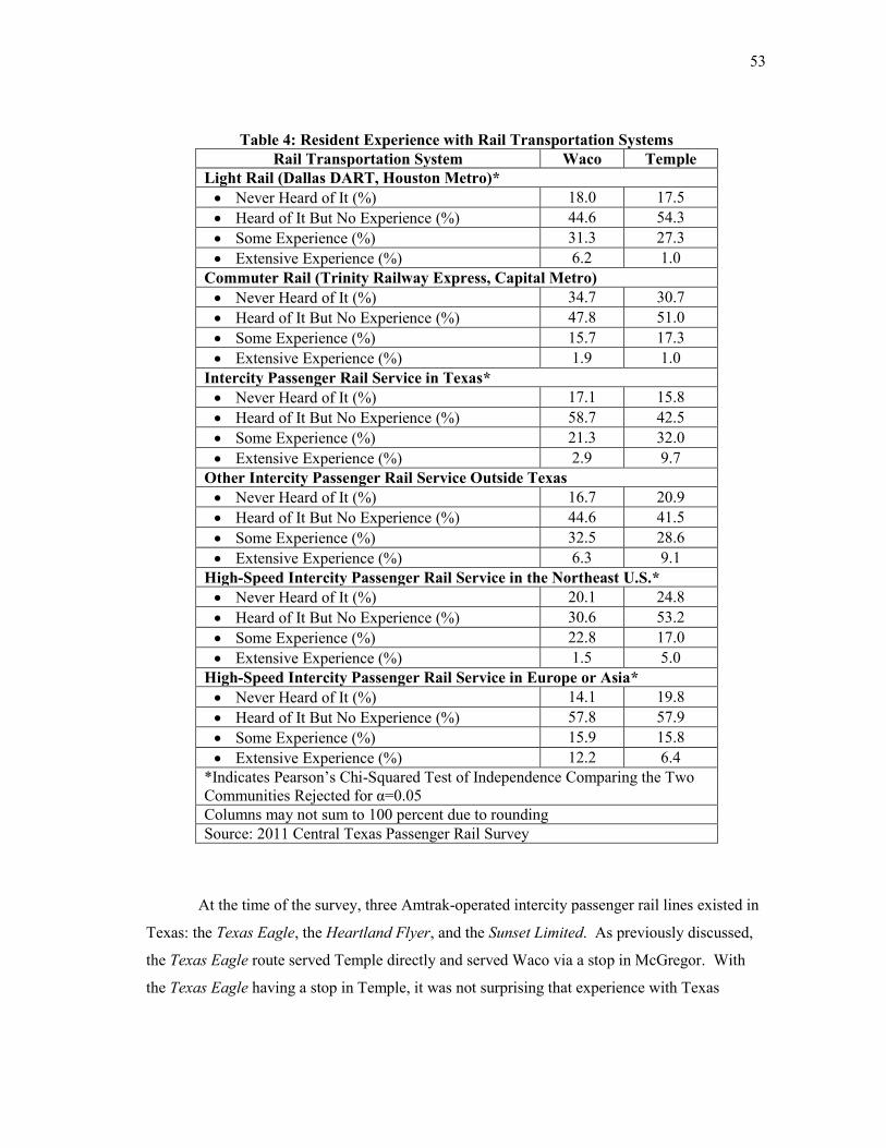
53
Table 4: Resident Experience with Rail Transportation Systems
Rail Transportation System Waco Temple
Light Rail (Dallas DART, Houston Metro)*
Never Heard of It (%) 18.0 17.5
Heard of It But No Experience (%) 44.6 54.3
Some Experience (%) 31.3 27.3
Extensive Experience (%) 6.2 1.0
Commuter Rail (Trinity Railway Express, Capital Metro)
Never Heard of It (%) 34.7 30.7
Heard of It But No Experience (%) 47.8 51.0
Some Experience (%) 15.7 17.3
Extensive Experience (%) 1.9 1.0
Intercity Passenger Rail Service in Texas*
Never Heard of It (%) 17.1 15.8
Heard of It But No Experience (%) 58.7 42.5
Some Experience (%) 21.3 32.0
Extensive Experience (%) 2.9 9.7
Other Intercity Passenger Rail Service Outside Texas
Never Heard of It (%) 16.7 20.9
Heard of It But No Experience (%) 44.6 41.5
Some Experience (%) 32.5 28.6
Extensive Experience (%) 6.3 9.1
High-Speed Intercity Passenger Rail Service in the Northeast U.S.*
Never Heard of It (%) 20.1 24.8
Heard of It But No Experience (%) 30.6 53.2
Some Experience (%) 22.8 17.0
Extensive Experience (%) 1.5 5.0
High-Speed Intercity Passenger Rail Service in Europe or Asia*
Never Heard of It (%) 14.1 19.8
Heard of It But No Experience (%) 57.8 57.9
Some Experience (%) 15.9 15.8
Extensive Experience (%) 12.2 6.4
*Indicates Pearson’s Chi-Squared Test of Independence Comparing the Two
Communities Rejected for α=0.05
Columns may not sum to 100 percent due to rounding
Source: 2011 Central Texas Passenger Rail Survey
At the time of the survey, three Amtrak-operated intercity passenger rail lines existed in
Texas: the Texas Eagle, the Heartland Flyer, and the Sunset Limited. As previously discussed,
the Texas Eagle route served Temple directly and served Waco via a stop in McGregor. With
the Texas Eagle having a stop in Temple, it was not surprising that experience with Texas
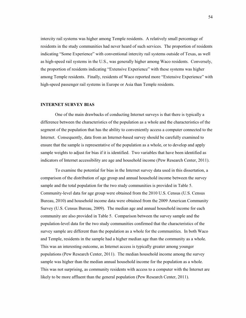
54
intercity rail systems was higher among Temple residents. A relatively small percentage of
residents in the study communities had never heard of such services. The proportion of residents
indicating “Some Experience” with conventional intercity rail systems outside of Texas, as well
as high-speed rail systems in the U.S., was generally higher among Waco residents. Conversely,
the proportion of residents indicating “Extensive Experience” with these systems was higher
among Temple residents. Finally, residents of Waco reported more “Extensive Experience” with
high-speed passenger rail systems in Europe or Asia than Temple residents.
INTERNET SURVEY BIAS
One of the main drawbacks of conducting Internet surveys is that there is typically a
difference between the characteristics of the population as a whole and the characteristics of the
segment of the population that has the ability to conveniently access a computer connected to the
Internet. Consequently, data from an Internet-based survey should be carefully examined to
ensure that the sample is representative of the population as a whole, or to develop and apply
sample weights to adjust for bias if it is identified. Two variables that have been identified as
indicators of Internet accessibility are age and household income (Pew Research Center, 2011).
To examine the potential for bias in the Internet survey data used in this dissertation, a
comparison of the distribution of age group and annual household income between the survey
sample and the total population for the two study communities is provided in Table 5.
Community-level data for age group were obtained from the 2010 U.S. Census (U.S. Census
Bureau, 2010) and household income data were obtained from the 2009 American Community
Survey (U.S. Census Bureau, 2009). The median age and annual household income for each
community are also provided in Table 5. Comparison between the survey sample and the
population-level data for the two study communities confirmed that the characteristics of the
survey sample are different than the population as a whole for the communities. In both Waco
and Temple, residents in the sample had a higher median age than the community as a whole.
This was an interesting outcome, as Internet access is typically greater among younger
populations (Pew Research Center, 2011). The median household income among the survey
sample was higher than the median annual household income for the population as a whole.
This was not surprising, as community residents with access to a computer with the Internet are
likely to be more affluent than the general population (Pew Research Center, 2011).
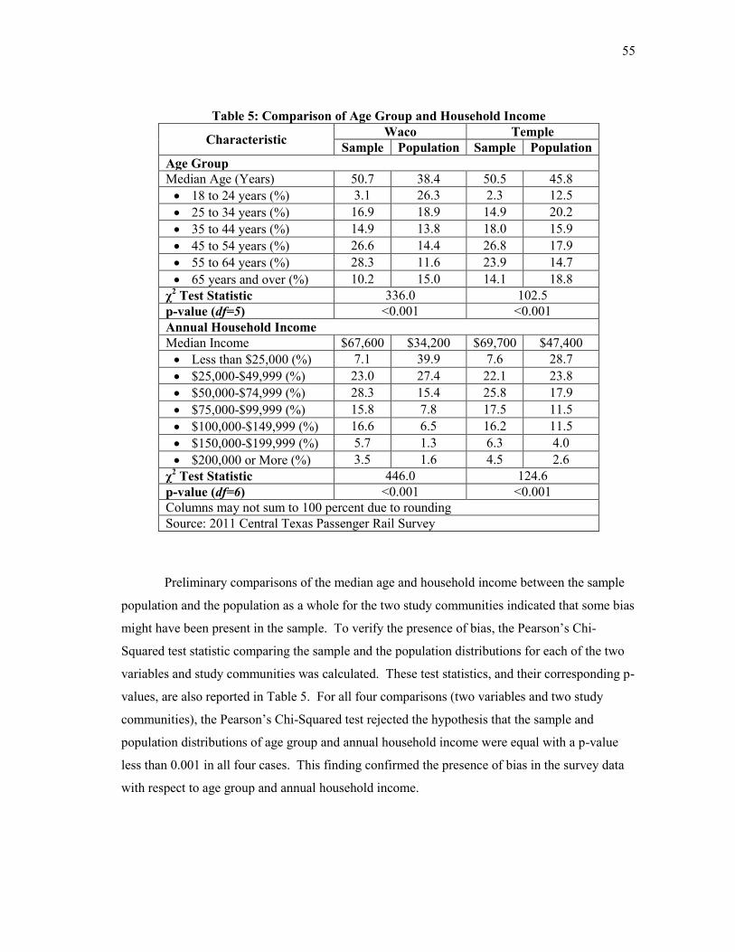
55
Table 5: Comparison of Age Group and Household Income
Characteristic Waco Temple
Sample Population Sample Population
Age Group
Median Age (Years) 50.7 38.4 50.5 45.8
18 to 24 years (%) 3.1 26.3 2.3 12.5
25 to 34 years (%) 16.9 18.9 14.9 20.2
35 to 44 years (%) 14.9 13.8 18.0 15.9
45 to 54 years (%) 26.6 14.4 26.8 17.9
55 to 64 years (%) 28.3 11.6 23.9 14.7
65 years and over (%) 10.2 15.0 14.1 18.8
χ2 Test Statistic 336.0 102.5
p-value (df=5) <0.001 <0.001
Annual Household Income
Median Income $67,600 $34,200 $69,700 $47,400
Less than $25,000 (%) 7.1 39.9 7.6 28.7
$25,000-$49,999 (%) 23.0 27.4 22.1 23.8
$50,000-$74,999 (%) 28.3 15.4 25.8 17.9
$75,000-$99,999 (%) 15.8 7.8 17.5 11.5
$100,000-$149,999 (%) 16.6 6.5 16.2 11.5
$150,000-$199,999 (%) 5.7 1.3 6.3 4.0
$200,000 or More (%) 3.5 1.6 4.5 2.6
χ2 Test Statistic 446.0 124.6
p-value (df=6) <0.001 <0.001
Columns may not sum to 100 percent due to rounding
Source: 2011 Central Texas Passenger Rail Survey
Preliminary comparisons of the median age and household income between the sample
population and the population as a whole for the two study communities indicated that some bias
might have been present in the sample. To verify the presence of bias, the Pearson’s Chi-
Squared test statistic comparing the sample and the population distributions for each of the two
variables and study communities was calculated. These test statistics, and their corresponding p-
values, are also reported in Table 5. For all four comparisons (two variables and two study
communities), the Pearson’s Chi-Squared test rejected the hypothesis that the sample and
population distributions of age group and annual household income were equal with a p-value
less than 0.001 in all four cases. This finding confirmed the presence of bias in the survey data
with respect to age group and annual household income.

56
Given the existence of bias in the survey sample, it was necessary to calculate a set of
sample weights to adjust the survey responses to reflect the community-level distributions of age
group and household income. Using the population-level distributions of age group and annual
household income (as reported in Table 5), a raking algorithm (Brackstone and Rao, 1976;
Deming and Stephan, 1940; Lohr, 2010) was used to compute community-specific sample
weights for each age group and annual household income pair contained in the sample. The
raking algorithm was necessary in this case because only the marginal distributions of
community-level age group and annual household income were available. The raking algorithm
computed the sample weights with precision to the third (0.001) decimal place. The sample
weights ranged between 0.161 and 15.459 for survey responses from Waco (see Table 6) and
between 0.406 and 13.459 for survey responses from Temple (see Table 7). Detailed sample
calculations for the survey sample weights from each community can be found in Appendix G.
Table 6: Survey Sample Weights: Waco
Age Group/
Household
Income Les
s th
an
$25,0
00
$25,0
00-
$49,9
99
$50,0
00-
$74,9
99
$75,0
00-
$99,9
99
$100,0
00-
$149,9
99
$150,0
00-
$199,9
99
$200,0
00
or
More
18 to 24 years 15.459 4.511 2.517 0.000 1.954 0.000 0.000
25 to 34 years 4.093 1.194 0.666 0.634 0.517 0.326 0.600
35 to 44 years 4.667 1.362 0.760 0.723 0.590 0.372 0.684
45 to 54 years 2.571 0.750 0.419 0.398 0.325 0.205 0.377
55 to 64 years 2.016 0.588 0.328 0.312 0.255 0.161 0.295
65 years and over 4.550 1.328 0.741 0.705 0.575 0.363 0.667
Table 7: Survey Sample Weights: Temple
Age Group/
Household
Income Les
s th
an
$2
5,0
00
$2
5,0
00-
$4
9,9
99
$5
0,0
00-
$7
4,9
99
$7
5,0
00-
$9
9,9
99
$1
00
,00
0-
$1
49
,99
9
$1
50
,00
0-
$1
99
,99
9
$2
00
,00
0
or
More
18 to 24 years 13.459 3.770 0.000 2.584 3.165 2.521 0.000
25 to 34 years 4.589 1.285 0.994 0.881 1.079 0.859 0.000
35 to 44 years 3.158 0.885 0.684 0.606 0.743 0.591 0.683
45 to 54 years 2.387 0.669 0.517 0.458 0.561 0.447 0.516
55 to 64 years 2.169 0.608 0.470 0.416 0.510 0.406 0.469
65 years and over 4.658 1.305 1.009 0.894 1.095 0.872 1.008
57
PRELIMINARY DATA ANALYSIS
The preliminary analysis encompassed two areas. First, the two stated preference
experimental designs considered in this dissertation, the d-efficient design and the adaptive
design, are evaluated for non-trading and lexicographic behavior. Second, the effect of varying
the visual representation of the hypothetical intercity passenger rail travel alternative is examined
in terms of various measures of survey behavior and survey response. From this point forward,
all analyses performed and results reported utilize weighted survey responses.
Non-Trading and Lexicographic Behavior
One of the fundamental assumptions of survey research is that the responses provided to
a survey questionnaire are the result of a legitimate decision-making process on the part of the
respondent. For many types of questions, the analyst has little basis for questioning whether or
not a given response is legitimate, other than easily recognized incongruent or extreme answers.
However, for stated preference questions, there are measures that the analyst can use to examine
if the responses provided to stated preference questions are the byproduct of a legitimate
decision-making process on the part of the respondent or if there are other factors that may be
influencing the responses. Two such measures, non-trading and lexicographic behavior, were
examined in this dissertation. While recognizing that some instances of non-trading and
lexicographic behavior resulting from a legitimate decision-making process will be present in a
set of stated preference responses, it is desirable to utilize stated preference designs that
minimize the occurrence of non-trading and lexicographic behavior.
Three measures of non-trading and lexicographic behavior were examined in this
dissertation: the percent of respondents always choosing automobile, the percent of respondents
always choosing train, and the percent of respondents always choosing the least expensive
alternative. It is noted that in all cases, the fastest alternative was the train and therefore the
metric “Always Choosing Train” would be equal to the “Always Choosing Fastest Alternative”
metric that is typically included in analyses of lexicographic behavior. The percent of
respondents for each measure for the two stated preference designs considered in this
dissertation is given in Table 8.
For the d-efficient stated preference design, instances of non-trading and lexicographic
behavior were detected in approximately one-quarter of the respondents. For the adaptive stated
preference design, approximately one out of every six respondents always selected the same

58
mode while less than 10 percent always selected the cheapest option. For the three measures
considered in Table 8, the null hypothesis that the proportion of respondents engaging in non-
trading or lexicographic behavior was equal between the two stated preference experimental
designs was rejected, with p<0.001 in all three cases. Therefore, it was concluded that the
adaptive design performed significantly better than the d-efficient design on the measures of
non-trading and lexicographic behavior considered here.
Table 8: Non-Trading and Lexicographic Behavior by Stated Preference Design
D-Efficient
Design
Adaptive
Design P-Value
Always Choosing Automobile (%) 24.6 18.4 <0.001
Always Choosing Train (%) 25.3 15.6 <0.001
Always Choosing Cheapest Alternative (%) 26.4 9.9 <0.001
The favorable performance of the adaptive design was probably due, in part, to the
algorithm used to select the attribute levels displayed in the adaptive questions. Specifically, by
adjusting the attributes of the two alternatives based on which alternative was selected in the
previous question, it was more difficult for a respondent to engage in lexicographic behavior (i.e.
choose the same mode or the cheapest mode in all three questions) without being required to
accept a larger trade-off in the attributes.
Visualization Effects
The survey randomly-assigned respondents to one of three visualization packages
describing a proposed intercity passenger train in the respondent’s home community. The three
packages were a “text-only” description of the rail service, a photo package portraying “typical”
train equipment (see Figure 3) to supplement the text description, and a photo package
portraying “flashy” train equipment to supplement the text description (see Figure 4). The
percentage of all respondents and respondents from each of the two study communities viewing
each visualization package is shown in Table 9. Approximately one-third of respondents across
the two study communities viewed each visualization package. A slightly higher percentage of
Temple respondents viewed the text-only package while a slightly higher percentage of Waco
residents viewed the “flashy” image package. Nevertheless, the Pearson’s Chi-Squared test
comparing the proportion of respondents in each study community viewing each version of the

59
survey was not rejected (χ2=4.813, p=0.09), confirming that a similar percentage of respondents
in each community were randomly-assigned to view one of the three image packages.
Table 9: Selected Survey Behavior Measures by Visualization Package
Survey Behavior Measure Text-Only vs. Images Typical vs. Flashy
Text Images P-Value Typical Flashy P-Value
All Respondents Viewing 32.90% 67.10% N/A 33.14% 33.97% N/A
Waco Respondents Viewing 30.92% 69.08% N/A 32.25% 36.83% N/A
Temple Respondents Viewing 35.31% 64.69% N/A 34.22% 30.47% N/A
Average # of Times
Rail Selected 3.11 3.09 0.978 3.05 3.11 0.638
Average Auto Travel
Time Presented (Minutes) 105.8 104.1 <0.001 105.4 102.7 <0.001
Average Auto
Travel Cost Presented $21.18 $21.04 0.279 $21.17 $20.92 0.088
Average Rail Travel
Time Presented (Minutes) 62.5 61.9 0.017 62.4 61.4 <0.001
Average Rail
Travel Cost Presented $28.30 $27.93 0.032 $27.93 $27.93 0.989
Average Rail
Headway Presented (Hours) 5.8 5.9 0.238 5.9 5.9 0.923
The presence of an image and the quality of the equipment portrayed could influence
stated preference survey responses and the resulting modeling outcomes. For example, images
of the rail service might influence the outcome of the stated preference survey by compelling
more respondents to select the train alternative if the photo is shown, and that the “Flashy”
image package would result in more respondents choosing the train alternative than the
“Typical” image package. The average number of times that the respondent selected “Train”
across the six stated preference exercises in the survey is shown in Table 9. Two comparisons
are provided: a comparison between the text-only version and versions with images (combined
“Typical” and “Flashy” image packages) and a comparison between the two versions with
images (comparison of “Typical” and “Flashy” image packages). The results shown in Table 9
indicate that neither the presence of the images, nor the quality of the equipment shown in the
images, had any significant effect on the number of times the train alternative was selected
across the six stated preference exercises (p=0.844 and p=0.638, respectively). This finding is a

60
preliminary indication that including photos in a stated preference survey does not have a
significant effect on the number of times a respondent selects the mode shown in the photo.
Also reported in Table 9 are the average travel time, travel cost, and rail service
headway across the three image packages, comparing the text-only version to the versions with
images as well as comparing the two versions with images. This comparison is important
because if the attributes are not equal across the three image packages, it may be difficult to
isolate the effect of visualization on discrete mode choice modeling outcomes. For both travel
alternatives, the average travel time displayed in the six stated preference exercises for
respondents viewing the “flashy” image package was significantly lower than for respondents
viewing the “typical” package. This difference resulted in the comparison of average travel time
between the text-only package and the two image packages being significant as well. Since
these differences affect the automobile and rail travel time attributes in the same way, the impact
on the subsequent discrete mode choice model analysis should be negligible. However, the rail
travel cost for the two image packages combined was significantly lower than the rail travel cost
for the text-only package. The difference in the presented rail fare between the two versions of
the survey (37 cents) was statistically significant but the practical significance of this difference
is probably negligible. Nevertheless, this issue may be worth additional investigation during the
travel mode choice model analysis presented in the next chapter.
The average value for each of the five attributes in the stated preference exercise by
visualization package (text-only vs. images, typical vs. flashy) and the mode selected by the
respondent (auto or rail) is shown in Table 10. It is expected that the average value of an
attribute for a particular mode among respondents choosing that mode would be lower than the
average value of the same attribute and mode among respondents not choosing that mode. For
example, if travel cost is a significant influence on mode choice, it would be expected that the
average travel cost for the auto alternative among respondents that selected auto would be lower
than the average travel cost for the auto alternative among respondents that selected rail. Among
all surveys, the average attribute values were significantly different in the proper direction for
four of the five attributes considered (no significant difference observed in X1, auto travel time).
The comparisons shown in Table 10 provide additional insight into the possible effects
of visualization on the stated preference responses. Specifically, it is possible that the presence
of images may have influenced the stated preference responses in such a way that the average
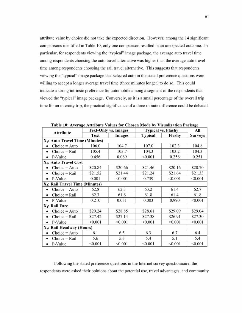
61
attribute value by choice did not take the expected direction. However, among the 14 significant
comparisons identified in Table 10, only one comparison resulted in an unexpected outcome. In
particular, for respondents viewing the “typical” image package, the average auto travel time
among respondents choosing the auto travel alternative was higher than the average auto travel
time among respondents choosing the rail travel alternative. This suggests that respondents
viewing the “typical” image package that selected auto in the stated preference questions were
willing to accept a longer average travel time (three minutes longer) to do so. This could
indicate a strong intrinsic preference for automobile among a segment of the respondents that
viewed the “typical” image package. Conversely, as it is a small percentage of the overall trip
time for an intercity trip, the practical significance of a three minute difference could be debated.
Table 10: Average Attribute Values for Chosen Mode by Visualization Package
Attribute Text-Only vs. Images Typical vs. Flashy All
Surveys Text Images Typical Flashy
X1: Auto Travel Time (Minutes)
Choice = Auto 106.0 104.7 107.0 102.3 104.8
Choice = Rail 105.4 103.7 104.3 103.2 104.3
P-Value 0.456 0.069 <0.001 0.256 0.251
X2: Auto Travel Cost
Choice = Auto $20.84 $20.66 $21.46 $20.16 $20.70
Choice = Rail $21.52 $21.44 $21.24 $21.64 $21.33
P-Value 0.001 <0.001 0.739 <0.001 <0.001
X3: Rail Travel Time (Minutes)
Choice = Auto 62.8 62.3 63.2 61.4 62.7
Choice = Rail 62.3 61.6 61.8 61.4 61.8
P-Value 0.210 0.031 0.003 0.990 <0.001
X4: Rail Fare
Choice = Auto $29.24 $28.85 $28.61 $29.09 $29.04
Choice = Rail $27.42 $27.14 $27.38 $26.91 $27.30
P-Value <0.001 <0.001 <0.001 <0.001 <0.001
X5: Rail Headway (Hours)
Choice = Auto 6.1 6.5 6.3 6.7 6.4
Choice = Rail 5.6 5.3 5.4 5.1 5.4
P-Value <0.001 <0.001 <0.001 <0.001 <0.001
Following the stated preference questions in the Internet survey questionnaire, the
respondents were asked their opinions about the potential use, travel advantages, and community
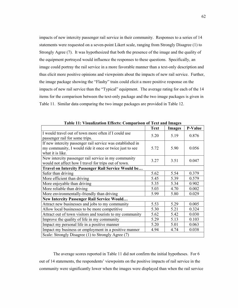
62
impacts of new intercity passenger rail service in their community. Responses to a series of 14
statements were requested on a seven-point Likert scale, ranging from Strongly Disagree (1) to
Strongly Agree (7). It was hypothesized that both the presence of the image and the quality of
the equipment portrayed would influence the responses to these questions. Specifically, an
image could portray the rail service in a more favorable manner than a text-only description and
thus elicit more positive opinions and viewpoints about the impacts of new rail service. Further,
the image package showing the “Flashy” train could elicit a more positive response on the
impacts of new rail service than the “Typical” equipment. The average rating for each of the 14
items for the comparison between the text-only package and the two image packages is given in
Table 11. Similar data comparing the two image packages are provided in Table 12.
Table 11: Visualization Effects: Comparison of Text and Images
Text Images P-Value
I would travel out of town more often if I could use
passenger rail for some trips. 5.20 5.19 0.876
If new intercity passenger rail service was established in
my community, I would ride it once or twice just to see
what it is like.
5.72 5.90 0.056
New intercity passenger rail service in my community
would not affect how I travel for trips out of town. 3.27 3.51 0.047
Travel on Intercity Passenger Rail Service Would be…
Safer than driving 5.62 5.54 0.379
More efficient than driving 5.45 5.39 0.579
More enjoyable than driving 5.35 5.34 0.902
More reliable than driving 5.03 4.70 0.002
More environmentally-friendly than driving 5.99 5.80 0.029
New Intercity Passenger Rail Service Would…
Attract new businesses and jobs to my community 5.53 5.29 0.005
Allow local businesses to be more competitive 5.30 5.21 0.324
Attract out of town visitors and tourists to my community 5.62 5.42 0.030
Improve the quality of life in my community 5.29 5.13 0.103
Impact my personal life in a positive manner 5.20 5.01 0.063
Impact my business or employment in a positive manner 4.94 4.74 0.038
Scale: Strongly Disagree (1) to Strongly Agree (7)
The average scores reported in Table 11 did not confirm the initial hypotheses. For 6
out of 14 statements, the respondents’ viewpoints on the positive impacts of rail service in the
community were significantly lower when the images were displayed than when the rail service

63
was described only with text (α=0.05). Contrary to prior expectations, the presence of images
appeared to actually lower the respondents’ opinions of the impacts of new intercity passenger
rail service on travel and in the local community. Specifically, respondents’ opinions on the
reliability and environmental advantages of rail travel compared with driving, as well as the role
of rail service in attracting new business and jobs, attracting out-of-town visitors and tourists, or
impacting the respondents’ business or employment in a positive manner, were lower for
respondents viewing one of the image packages, as compared to the text-only description.
The only instance where the scores were higher for the image packages was for the
following statement: “If new intercity passenger rail service was established in my community, I
would ride it once or twice just to see what it is like.” This statement was included as a possible
indicator of possible novelty-induced travel on the new intercity passenger rail service in the
respondent’s home community (Gunn et al., 1992; Kanafani and Youssef, 1993). Although not
significant (p=0.056), the average score for this item for respondents viewing either of the image
packages (5.90/7) was higher than the score for the text-only respondents (5.72/7).
Table 12: Visualization Effects: Comparison of Two Image Packages
Typical Flashy P-Value
I would travel out of town more often if I could use
passenger rail for some trips. 5.15 5.21 0.617
If new intercity passenger rail service was established in
my community, I would ride it once or twice just to see
what it is like.
5.82 5.98 0.103
New intercity passenger rail service in my community
would not affect how I travel for trips out of town. 3.69 3.34 0.010
Travel on Intercity Passenger Rail Service Would be…
Safer than driving 5.48 5.60 0.254
More efficient than driving 5.24 5.54 0.009
More enjoyable than driving 5.38 5.30 0.499
More reliable than driving 4.79 4.61 0.136
More environmentally-friendly than driving 5.72 5.87 0.137
New Intercity Passenger Rail Service Would…
Attract new businesses and jobs to my community 5.40 5.18 0.025
Allow local businesses to be more competitive 5.29 5.14 0.133
Attract out of town visitors and tourists to my community 5.43 5.42 0.971
Improve the quality of life in my community 5.28 4.99 0.011
Impact my personal life in a positive manner 5.11 4.91 0.077
Impact my business or employment in a positive manner 4.89 4.59 0.008
Scale: Strongly Disagree (1) to Strongly Agree (7)

64
Comparing the average scores between the “Typical” and “Flashy” image packages
(Table 12) indicated that only 5 out of the 14 statements differed significantly on their average
scores across the two image packages. For the item “new intercity passenger rail service would
not affect how I travel for trips out of town,” respondents viewing the “Typical” image package
had a higher average score on this item (3.69/7) than respondents viewing the “Flashy” package
(3.34/7). Respondents viewing the “Flashy” image package scored the item “more efficient than
driving” significantly higher (5.54/7) than respondents viewing the “Typical” package (5.24/7).
Finally, respondents viewing the “Typical” package had higher average scores than respondents
viewing the “Flashy” image package for the impacts of new intercity passenger rail service on
local business and the overall quality of life in the respondent’s home community.
Table 13: Comparison of Opinion Question Scores by Choice
Choice =
Auto
Choice =
Rail P-Value
I would travel out of town more often if I could use
passenger rail for some trips. 4.60 5.73 <0.001
If new intercity passenger rail service was established in
my community, I would ride it once or twice just to see
what it is like.
5.53 6.14 <0.001
New intercity passenger rail service in my community
would not affect how I travel for trips out of town. 3.79 3.10 <0.001
Travel on Intercity Passenger Rail Service Would be…
Safer than driving 5.20 5.90 <0.001
More efficient than driving 4.93 5.85 <0.001
More enjoyable than driving 4.91 5.75 <0.001
More reliable than driving 4.35 5.22 <0.001
More environmentally-friendly than driving 5.55 6.16 <0.001
New Intercity Passenger Rail Service Would…
Attract new businesses and jobs to my community 4.99 5.72 <0.001
Allow local businesses to be more competitive 4.84 5.61 <0.001
Attract out of town visitors and tourists to my community 5.09 5.86 <0.001
Improve the quality of life in my community 4.73 5.60 <0.001
Impact my personal life in a positive manner 4.52 5.57 <0.001
Impact my business or employment in a positive manner 4.41 5.16 <0.001
Scale: Strongly Disagree (1) to Strongly Agree (7)
Another item of interest for the preliminary analysis is the possible relationship between
the responses to the 14 resident opinion items and the mode selected by the respondent (auto or

65
rail) in the stated preference questions. It would be expected a priori that respondents who
selected rail in these questions would have a more favorable opinion about the travel benefits
and community impacts of rail service, and vice versa for respondents who selected auto in the
stated preference questions. A comparison of the average rating for each of the 14 items by
mode selected by the respondent in the stated preference questions (auto or rail) is shown in
Table 13. As expected, respondents that selected rail in the stated preference questions had more
favorable opinions of travel by rail instead of automobile and the community impacts of
potential new intercity passenger rail service in their home community than respondents that
selected auto. These differences were highly significant (p<0.001) across all 14 items,
suggesting a strong relationship between the mode selected in the stated preference questions
and the respondents’ opinions of intercity passenger rail service.
SUMMARY
This chapter presented a preliminary analysis of the data obtained from a survey of
residents in Waco and Temple, Texas. Responses to the survey indicated that a majority of
surveyed residents in both communities had made a personal trip in an automobile to the Dallas
region in the last six months, providing at least some familiarity with the hypothetical situation
presented in the stated preference section of the survey. As expected with an Internet survey,
there was a significant difference detected between the survey sample and the overall community
population in both Waco and Temple. Specifically, the distributions of age group and annual
household income between the sample and the overall population were significantly different.
As a result of this bias, a raking algorithm was used to calculate a set of sample weights for
respondents in each age group and annual household income level by community, in turn better
representing the opinions and preferences of the residents of each community. These weights
were applied to findings in the remainder of the preliminary analysis and will be applied to the
discrete choice modeling analysis and other analysis presented in the following chapter.
Preliminary comparisons between the two stated preference experimental design
approaches considered in this dissertation (the d-efficient design and the adaptive design)
indicated that the adaptive design performed significantly better than the d-efficient design on
selected measures of non-trading and lexicographic behavior. Based on these preliminary
findings, there is evidence to suggest that mode choice models constructed using data from the

66
adaptive stated preference questions will be superior to models constructed with the d-efficient
data in terms of model fit, parameter stability, and predictive capability.
Preliminary comparisons of the three image packages, however, demonstrated mixed
results. In terms of survey behavior, respondents viewing one of the two image packages did not
choose the train alternative in the stated preference questions significantly more than the text-
only respondents. Average scores for 14 statements related to the impacts of new rail service on
intercity travel and overall community impacts found that respondents viewing the text-only
description had a slightly more favorable view of the new rail service than respondents viewing
one of the two image packages; however, few significant differences between the “Typical” and
the “Flashy” image packages were detected. The influence of the actual stated preference
questions themselves on these findings could have also been a confounding factor. For example,
given the position of the 14 resident opinion items on the survey (immediately following the
stated preference questions), it is possible that the time, cost, and service headway parameters
presented in the stated preference questions (in addition to the visualization of potential train
equipment) influenced the respondent’s perception of proposed intercity passenger rail service
and thus the responses provided on the resident opinion items. Based on these preliminary
findings, there is limited evidence to suggest that the presence or quality of images presented to
the respondent prior to the stated preference exercise will have a significant influence on the
quality of resulting discrete travel mode choice models.
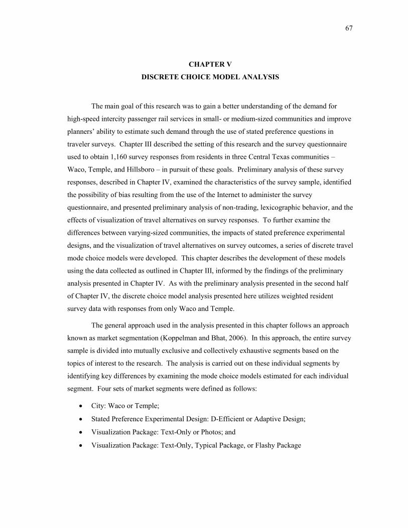
67
CHAPTER V
DISCRETE CHOICE MODEL ANALYSIS
The main goal of this research was to gain a better understanding of the demand for
high-speed intercity passenger rail services in small- or medium-sized communities and improve
planners’ ability to estimate such demand through the use of stated preference questions in
traveler surveys. Chapter III described the setting of this research and the survey questionnaire
used to obtain 1,160 survey responses from residents in three Central Texas communities –
Waco, Temple, and Hillsboro – in pursuit of these goals. Preliminary analysis of these survey
responses, described in Chapter IV, examined the characteristics of the survey sample, identified
the possibility of bias resulting from the use of the Internet to administer the survey
questionnaire, and presented preliminary analysis of non-trading, lexicographic behavior, and the
effects of visualization of travel alternatives on survey responses. To further examine the
differences between varying-sized communities, the impacts of stated preference experimental
designs, and the visualization of travel alternatives on survey outcomes, a series of discrete travel
mode choice models were developed. This chapter describes the development of these models
using the data collected as outlined in Chapter III, informed by the findings of the preliminary
analysis presented in Chapter IV. As with the preliminary analysis presented in the second half
of Chapter IV, the discrete choice model analysis presented here utilizes weighted resident
survey data with responses from only Waco and Temple.
The general approach used in the analysis presented in this chapter follows an approach
known as market segmentation (Koppelman and Bhat, 2006). In this approach, the entire survey
sample is divided into mutually exclusive and collectively exhaustive segments based on the
topics of interest to the research. The analysis is carried out on these individual segments by
identifying key differences by examining the mode choice models estimated for each individual
segment. Four sets of market segments were defined as follows:
City: Waco or Temple;
Stated Preference Experimental Design: D-Efficient or Adaptive Design;
Visualization Package: Text-Only or Photos; and
Visualization Package: Text-Only, Typical Package, or Flashy Package

68
Given this segmentation of the entire survey data set, the discrete travel mode choice model
analysis presented in this chapter was undertaken using the following procedure:
Identification of candidate variables for the mode choice model;
Specification and estimation of a preliminary multinomial logit (MNL) model from the
whole survey sample containing significant variables as identified;
Estimation of a corresponding mixed logit (ML) model containing the significant
variables identified from the preliminary MNL model from the previous step. Since this
model is estimated on the entire data set, this model is referred to as the “pooled” model;
Market segmentation analysis, as outlined by Koppelman and Bhat (2006), to determine
if the previously-identified segments are statistically different from each other based on
a comparison between the “pooled” ML model and an ML model of the same
specification fit to data from an individual segment; and
Specification and estimation of an optimal ML model for each segment.
One of the key outputs from discrete travel mode choice models is the traveler’s value of travel
time (VOT). VOT is important tool used in the economic analysis of transportation investments.
Recognizing the broader importance of the VOT for transportation planning and decision-
making, the final section of this chapter presents a more detailed analysis of the VOT differences
across the various market segments.
PRELIMINARY MODEL DEVELOPMENT
Variable Selection
The first step in the mode choice model analysis was to examine the survey data set for
variables that could potentially have a significant contribution to the model specification. A
preliminary mode choice model specification (given in the form of Equation (1)) was proposed
and presented in Equations (8) and (9), containing travel time and travel cost (for the auto and
rail modes) and the service headway (rail mode only). Building on this preliminary model
specification, it was necessary to identify additional variables of significance to the mode choice
model. Potential additional variables of interest for this model obtained from the resident survey
questionnaire included the following:
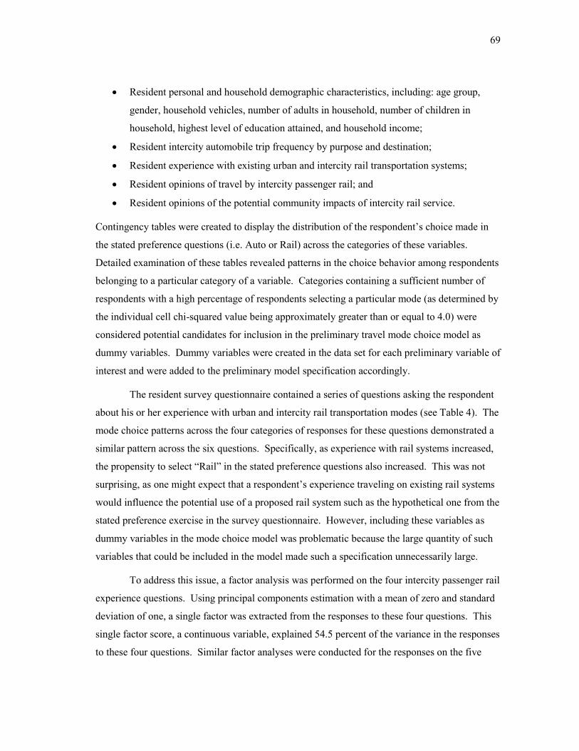
69
Resident personal and household demographic characteristics, including: age group,
gender, household vehicles, number of adults in household, number of children in
household, highest level of education attained, and household income;
Resident intercity automobile trip frequency by purpose and destination;
Resident experience with existing urban and intercity rail transportation systems;
Resident opinions of travel by intercity passenger rail; and
Resident opinions of the potential community impacts of intercity rail service.
Contingency tables were created to display the distribution of the respondent’s choice made in
the stated preference questions (i.e. Auto or Rail) across the categories of these variables.
Detailed examination of these tables revealed patterns in the choice behavior among respondents
belonging to a particular category of a variable. Categories containing a sufficient number of
respondents with a high percentage of respondents selecting a particular mode (as determined by
the individual cell chi-squared value being approximately greater than or equal to 4.0) were
considered potential candidates for inclusion in the preliminary travel mode choice model as
dummy variables. Dummy variables were created in the data set for each preliminary variable of
interest and were added to the preliminary model specification accordingly.
The resident survey questionnaire contained a series of questions asking the respondent
about his or her experience with urban and intercity rail transportation modes (see Table 4). The
mode choice patterns across the four categories of responses for these questions demonstrated a
similar pattern across the six questions. Specifically, as experience with rail systems increased,
the propensity to select “Rail” in the stated preference questions also increased. This was not
surprising, as one might expect that a respondent’s experience traveling on existing rail systems
would influence the potential use of a proposed rail system such as the hypothetical one from the
stated preference exercise in the survey questionnaire. However, including these variables as
dummy variables in the mode choice model was problematic because the large quantity of such
variables that could be included in the model made such a specification unnecessarily large.
To address this issue, a factor analysis was performed on the four intercity passenger rail
experience questions. Using principal components estimation with a mean of zero and standard
deviation of one, a single factor was extracted from the responses to these four questions. This
single factor score, a continuous variable, explained 54.5 percent of the variance in the responses
to these four questions. Similar factor analyses were conducted for the responses on the five

70
statements related to the respondent’s opinion of rail travel as compared to driving and six
statements related to the respondent’s opinion of the potential impacts of new intercity passenger
rail service on his or her home community. Table 14 displays the factor loadings of these initial
survey questions on each of the three factors, with each question sufficiently loading on its
respective factor score. The single “Rail Travel” factor explained 68.8 percent of the variance in
responses to that series of questions while the “Rail Community Impacts” factor explained 75.7
percent of the variance in responses to that series of questions.
Table 14: Factor Analysis of Rail Experience and Resident Opinion Responses
Extracted Factor Information
Variance Explained/
Factor Loading/
Factor Scores
Extracted Factor: Intercity Rail Experience Factor
Percent of Variance Explained with Single Factor 54.5%
Factor Loading: Intercity Passenger Rail Service in Texas 0.583
Factor Loading: Other Intercity Passenger Rail Outside Texas 0.832
Factor Loading: HSR Service in the Northeast U.S. 0.816
Factor Loading: HSR Service in Europe or Asia 0.693
Average Factor Score (Choice = Auto) -0.246
Average Factor Score (Choice = Rail) 0.004
Extracted Factor: Rail Travel Factor
Percent of Variance Explained with Single Extracted Factor 68.8%
Factor Loading: Safer than driving 0.833
Factor Loading: More efficient than driving 0.855
Factor Loading: More enjoyable than driving 0.854
Factor Loading: More reliable than driving 0.784
Factor Loading: More environmentally-friendly than driving 0.817
Average Factor Score (Choice = Auto) -0.315
Average Factor Score (Choice = Rail) 0.347
Extracted Factor: Rail Community Impacts Factor
Percent of Variance Explained with Single Extracted Factor 75.7%
Factor Loading: Attract new businesses and jobs to my community 0.898
Factor Loading: Allow local businesses to be more competitive 0.892
Factor Loading: Attract visitors and tourists to my community 0.860
Factor Loading: Improve the quality of life in my community 0.900
Factor Loading: Impact personal life in positive manner 0.874
Factor Loading: Impact business or employment in positive manner 0.794
Average Factor Score (Choice = Auto) -0.264
Average Factor Score (Choice = Rail) 0.405
71
Also shown in Table 14 is the average factor score for respondents choosing “Auto” or
“Rail” in the stated preference questions. Across the three factor scores, the average factor score
for respondents choosing rail was significantly higher than the average factor score for
respondents choosing auto (p<0.001 for all cases). Given these patterns, the inclusion of the
three factor scores as variables in the rail mode choice model was explored in the preliminary
model specification process. While variables like these (i.e. opinion questions) are not typically
included in mode choice models due to the inability to forecast such variables, they were
considered in this research because the model being developed in this dissertation was not being
used for a formal ridership analysis.
Preliminary Multinomial Logit Model Specification
After identifying a list of candidate dummy variables and extracting the three factor
analysis variables to be included in the mode choice model, the next step in the analysis was to
specify and estimate a preliminary MNL model. The computer software program NLOGIT™
(Greene, 2007) was used to estimate coefficients for the various model specifications. Selected
syntax used in the NLOGIT™ computer software program can be found in Appendix H.
To compare different model specifications, a number of metrics were identified and
examined, including the model log-likelihood, the adjusted rho-squared, the D-error, the A-error,
the percent of choices correctly predicted by the model, and the values of travel time and rail
service headway. Several of these measures are defined here for convenience. The adjusted rho-
squared is an overall goodness-of-fit measure defined by Equation (12) as follows:
Adjusted ρc2 = 1 -
sKCLL
KLL
)(
)( (12)
Where LL(β) = Log-Likelihood for the Estimated Model
LL(C) = Log-Likelihood for the Constants-Only Model
K = Number of Parameters in the Estimated Model
Ks = Number of Parameters in the Constants-Only Model (Ks = 1)
The adjusted ρ2 is symbolized with a subscript C (ρc
2) to indicate that it is calculated with respect
to the constant- or intercept-only model. A larger ρc2 is desired because it indicates a better fit of
72
the model to the data. The D-error is defined previously by Equation (7). The A-error is defined
by Equation (13) as follows:
A-Error = K
tr )( (13)
Where Ω = Asymptotic Variance-Covariance Matrix of the Estimated Model
K = Number of Parameters in the Estimated Model
Models with smaller D-error and A-error are desired. The implied VOT for the estimated model
is defined by Equation (14) as follows:
VOT = TC
TT
x 60 (14)
Where βTT = Travel Time Coefficient from the Estimated Model
βTC = Travel Cost Coefficient from the Estimated Model
Substituting (βFREQ) for (βTT) in Equation (14) allows for the estimate of the value of rail service
headway (VOF). However, the multiplicative constant (x 60) is not needed if the βFREQ is
already given in hours as its unit.
Starting with the base model specification given by Equations (8) and (9), candidate
dummy variables were added and removed from the model using an iterative process until a
suitable specification was located. The preliminary multinomial logit model parameter estimates
for the model estimated on all resident survey responses with the data weighted to reflect bias as
previously discussed are shown in Table 15. Consistent with prior expectations, the model log-
likelihood and the adjusted ρc2 increased as variables were added to the model. The inclusion of
six individual traveler dummy variables in the “All Data” model in Table 15 was a significant
improvement over the model with only the travel mode variables (χ2=386.8, df=6, p<0.001).
The addition of the three factor analysis (defined in Table 14) also represented a significant
improvement in the model only the individual traveler dummy variables and the travel mode
variables (χ2=1,598.2, df=3, p<0.001).
However, one glaring issue was noted with the parameter estimates of the “All Data”
model. Specifically, the travel time parameter was found to not contribute significantly to the
overall model (p=0.165). Travel mode choice models with key policy variables (i.e. travel time
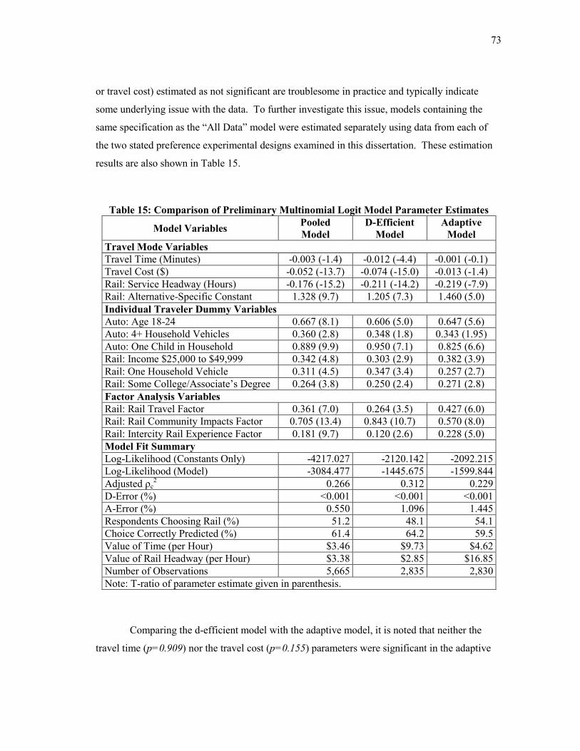
73
or travel cost) estimated as not significant are troublesome in practice and typically indicate
some underlying issue with the data. To further investigate this issue, models containing the
same specification as the “All Data” model were estimated separately using data from each of
the two stated preference experimental designs examined in this dissertation. These estimation
results are also shown in Table 15.
Table 15: Comparison of Preliminary Multinomial Logit Model Parameter Estimates
Model Variables Pooled
Model
D-Efficient
Model
Adaptive
Model
Travel Mode Variables
Travel Time (Minutes) -0.003 (-1.4) -0.012 (-4.4) -0.001 (-0.1)
Travel Cost ($) -0.052 (-13.7) -0.074 (-15.0) -0.013 (-1.4)
Rail: Service Headway (Hours) -0.176 (-15.2) -0.211 (-14.2) -0.219 (-7.9)
Rail: Alternative-Specific Constant 1.328 (9.7) 1.205 (7.3) 1.460 (5.0)
Individual Traveler Dummy Variables
Auto: Age 18-24 0.667 (8.1) 0.606 (5.0) 0.647 (5.6)
Auto: 4+ Household Vehicles 0.360 (2.8) 0.348 (1.8) 0.343 (1.95)
Auto: One Child in Household 0.889 (9.9) 0.950 (7.1) 0.825 (6.6)
Rail: Income $25,000 to $49,999 0.342 (4.8) 0.303 (2.9) 0.382 (3.9)
Rail: One Household Vehicle 0.311 (4.5) 0.347 (3.4) 0.257 (2.7)
Rail: Some College/Associate’s Degree 0.264 (3.8) 0.250 (2.4) 0.271 (2.8)
Factor Analysis Variables
Rail: Rail Travel Factor 0.361 (7.0) 0.264 (3.5) 0.427 (6.0)
Rail: Rail Community Impacts Factor 0.705 (13.4) 0.843 (10.7) 0.570 (8.0)
Rail: Intercity Rail Experience Factor 0.181 (9.7) 0.120 (2.6) 0.228 (5.0)
Model Fit Summary
Log-Likelihood (Constants Only) -4217.027 -2120.142 -2092.215
Log-Likelihood (Model) -3084.477 -1445.675 -1599.844
Adjusted ρc2 0.266 0.312 0.229
D-Error (%) <0.001 <0.001 <0.001
A-Error (%) 0.550 1.096 1.445
Respondents Choosing Rail (%) 51.2 48.1 54.1
Choice Correctly Predicted (%) 61.4 64.2 59.5
Value of Time (per Hour) $3.46 $9.73 $4.62
Value of Rail Headway (per Hour) $3.38 $2.85 $16.85
Number of Observations 5,665 2,835 2,830
Note: T-ratio of parameter estimate given in parenthesis.
Comparing the d-efficient model with the adaptive model, it is noted that neither the
travel time (p=0.909) nor the travel cost (p=0.155) parameters were significant in the adaptive
74
model but were found to be significant in the d-efficient model. It is also noted from Table 15
that the d-efficient model had a better overall fit (larger adjusted ρc2 and model log-likelihood)
than the adaptive model. Other variable combinations for the adaptive model resulted in similar
issues. Furthermore, model estimates that result in key policy variables (i.e. travel time or travel
cost) being insignificant are not useful (Ortúzar and Willumsen, 2001). On this basis, it was
determined that the adaptive responses contained data that made it unsuitable for travel mode
choice model estimation. Consequently, the adaptive responses were discarded and only the d-
efficient responses were used for subsequent analyses presented in the body of this dissertation.
Model parameter estimates by study community and image package for all data (both d-efficient
and adaptive design data) and with just the adaptive design data are provided in Appendix I.
Using only the d-efficient responses, a “Pooled Model” similar to the “D-Efficient
Model” in Table 15 was estimated. One individual traveler dummy variable, the “4+ Household
Vehicles” dummy variable on the auto choice model, was removed from the specification
because it was not significant. The four travel mode variables, five individual traveler dummy
variables, and the three factor analysis variables were retained. The full specification, parameter
estimates, t-ratios, and model statistics for the pooled MNL model are presented in Table 16.
Examining the parameter estimates in Table 16 indicates that all the parameters are
significant (i.e. |t-ratio| > 1.96); in particular, the t-ratios for the four travel mode variables are
large, indicating a strong contribution to the model. Additionally, all the variable signs are in the
expected direction (negative for the travel mode variables, positive for the individual traveler
dummy variables). The rail alternative-specific constant was significant and positive, indicating
an underlying preference for rail if all other variables are equal. Significant individual traveler
dummy variables in the auto choice model included age 18 to 24 and one child in household.
Based on the parameter estimates, the “one child in household variable” exerted a stronger
influence on the auto choice than the “age 18 to 24” variable. Significant individual traveler
dummy variables in the rail choice model included annual household income between $25,000
and $50,000, one household vehicle, and some college/Associate’s degree as highest level of
education attained. None of the individual traveler dummy variables in the rail choice model
stood out as being more influential than the others. The variable with the highest parameter
estimate in the rail choice model was the community impacts factor variable with β=0.853.
Parameter estimates corresponding to the other two factor analysis variables were significant and

75
had a positive sign, indicating that a higher score on these factors (i.e. a more favorable view of
rail service or greater experience) increased the probability of choosing rail, ceteris paribus.
From Equation (14), the implied VOT from the model in Table 16 is $9.73 per hour and the
implied VOF from this model is $2.84 per hour.
Table 16: Pooled Model Multinomial Logit Model (D-Efficient Data Only)
Model Variables Parameter
Estimate T-Ratio
Travel Mode Variables
Travel Time (Minutes) -0.012 -4.341
Travel Cost ($) -0.074 -14.995
Rail: Service Headway (Hours) -0.210 -14.182
Rail: Alternative-Specific Constant 1.166 7.098
Individual Traveler Dummy Variables
Auto: Age 18-24 0.594 4.892
Auto: One Child in Household 0.942 7.083
Rail: Income $25,000 to $49,999 0.320 3.088
Rail: One Household Vehicle 0.376 3.758
Rail: Some College/Associate’s Degree 0.242 2.353
Factor Analysis Variables
Rail: Rail Travel Factor 0.259 3.407
Rail: Rail Community Impacts Factor 0.853 10.913
Rail: Intercity Rail Experience Factor 0.117 2.502
Model Fit Summary
Log-Likelihood (Constants Only) -2120.142
Log-Likelihood (Model) -1447.362
Adjusted ρc2 0.313
D-Error (%) <0.001
A-Error (%) 0.875
Respondents Choosing Rail (%) 48.2
Choice Correctly Predicted (%) 64.3
Value of Time (per Hour) $9.73
Value of Rail Headway (per Hour) $2.84
Number of Observations 2,835
Preliminary Mixed Logit Model Estimation
In a stated preference survey, such as the resident survey questionnaire used in this
dissertation, it is typical to present a respondent with more than one stated preference exercise
for consideration. This is done because it is more efficient to gather multiple stated preference
76
observations from a single respondent than to have a single stated preference observation per
respondent and thus be required to obtain a larger number of respondents to generate a sufficient
sample size. While obtaining multiple stated preference observations from a single respondent is
typical practice, doing so presents an issue for the estimation of the classical multinomial logit
model. Specifically, multiple observations from a single individual introduce the possibility for
correlation across these observations. This correlation is a violation of the assumption that the
error term (εjs) in the utility model (see Equation (1)) is independent across observations.
To overcome this issue, a discrete choice model formulation known as the mixed logit
model can be used (Hensher and Greene, 2003; Revelt and Train, 1998; Train, 2009). In the
mixed logit model, the analyst specifies one or more parameters as random (thus leading to the
model also being known as the “random parameters” model) and assumes an underlying
distribution for the random term. Typical distributions can include the normal, lognormal,
uniform, or triangular. To estimate the mixed logit model, a specified number of random draws
is taken from the selected distribution and the random parameter(s) can be estimated along with
the standard deviation of the random parameter(s). Details on the specification and estimation of
the mixed logit model can be found in Hensher and Greene (2003) and Train (2009).
For the travel mode choice model considered in this dissertation, the travel time
parameter (βTT) was assumed to be a random parameter taking the form of a triangular
distribution. The triangular distribution is generated from a uniform distribution U (0,1). From
the uniform distribution, the triangular distribution is estimated by Equation (15) as follows:
t = 12 U , for U < 0.5
t = )1(21 U , otherwise (15)
Where t = Probability density function (PDF) for the triangular distribution
U = Random number from the uniform distribution U (0,1)
The resulting triangular distribution has a range between -1 and 1. The random parameter,
therefore, is estimated as follows:
t ˆˆ (16)
Where = Individual-specific random parameter estimate

77
= Mean random parameter estimate given by ML model
= Standard deviation of the random parameter estimate
t = PDF of the triangular distribution as given by Equation (15)
Since the sign of the travel time parameter is expected to be negative a priori, the use of the
standard deviation ( ) in Equation (16) can be problematic because there is a possibility that the
resulting parameter estimate could be positive. To overcome this, the analyst can constrain the
spread of the distribution to equal the mean. In this case, the random parameter is estimated with
a modified version of Equation (16) as follows:
t ˆˆ (17)
Where = Individual-specific random parameter estimate
= Mean random parameter estimate given by ML model
t = PDF of the triangular distribution as given by Equation (15)
Following Equation (17), the spread of the triangular distribution around the mean
parameter value (β) is constrained between 0 and 2β (i.e. values from the triangular distribution
between -1 and 1 multiplied by the estimated parameter β). Because of this constraint, the
random parameter will never assume a positive value and thus issues related to illogical (i.e.
negative) VOT estimates are avoided (Hensher and Greene, 2003; Train, 2009).
Using the travel time parameter (βTT) as a random parameter (Equation (17)), a mixed
logit model with the same specification as the multinomial logit model given in Table 16 was
estimated. These estimation results are given in Table 17. No other parameters in the model
were assumed to be random. Although it is typical for an alternative-specific constant to be
estimated in the form of a random parameter if it is included, this was not done here because it
resulted in unstable parameter estimates. To estimate the random parameter and its standard
deviation, 500 Halton or “intelligent” draws were used. Carlsson (2003) used 500 draws to
estimate random parameter logit models examining the use of high-speed intercity passenger rail
among business travelers in Sweden; however, he used random draws rather than Halton draws.
The use of Halton sequences instead of random draws decreases the estimation time and
smoothes the simulation output (Bhat, 2001; Hensher and Greene, 2003; Train, 2000).
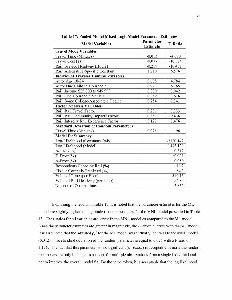
78
Table 17: Pooled Model Mixed Logit Model Parameter Estimates
Model Variables Parameter
Estimate T-Ratio
Travel Mode Variables
Travel Time (Minutes) -0.013 -4.080
Travel Cost ($) -0.077 -10.784
Rail: Service Headway (Hours) -0.219 -10.431
Rail: Alternative-Specific Constant 1.210 6.576
Individual Traveler Dummy Variables
Auto: Age 18-24 0.608 4.784
Auto: One Child in Household 0.993 6.265
Rail: Income $25,000 to $49,999 0.330 3.042
Rail: One Household Vehicle 0.389 3.676
Rail: Some College/Associate’s Degree 0.254 2.341
Factor Analysis Variables
Rail: Rail Travel Factor 0.271 3.333
Rail: Rail Community Impacts Factor 0.882 9.436
Rail: Intercity Rail Experience Factor 0.122 2.476
Standard Deviation of Random Parameters
Travel Time (Minutes) 0.025 1.196
Model Fit Summary
Log-Likelihood (Constants Only) -2120.142
Log-Likelihood (Model) -1447.129
Adjusted ρc2 0.312
D-Error (%) <0.001
A-Error (%) 0.989
Respondents Choosing Rail (%) 48.2
Choice Correctly Predicted (%) 64.3
Value of Time (per Hour) $10.13
Value of Rail Headway (per Hour) $2.84
Number of Observations 2,835
Examining the results in Table 17, it is noted that the parameter estimates for the ML
model are slightly higher in magnitude than the estimates for the MNL model presented in Table
16. The t-ratios for all variables are larger in the MNL model as compared to the ML model.
Since the parameter estimates are greater in magnitude, the A-error is larger with the ML model.
It is also noted that the adjusted ρc2 for the ML model was virtually identical to the MNL model
(0.312). The standard deviation of the random parameter is equal to 0.025 with a t-ratio of
1.196. The fact that this parameter is not significant (p=0.232) is acceptable because the random
parameters are only included to account for multiple observations from a single individual and
not to improve the overall model fit. By the same token, it is acceptable that the log-likelihood
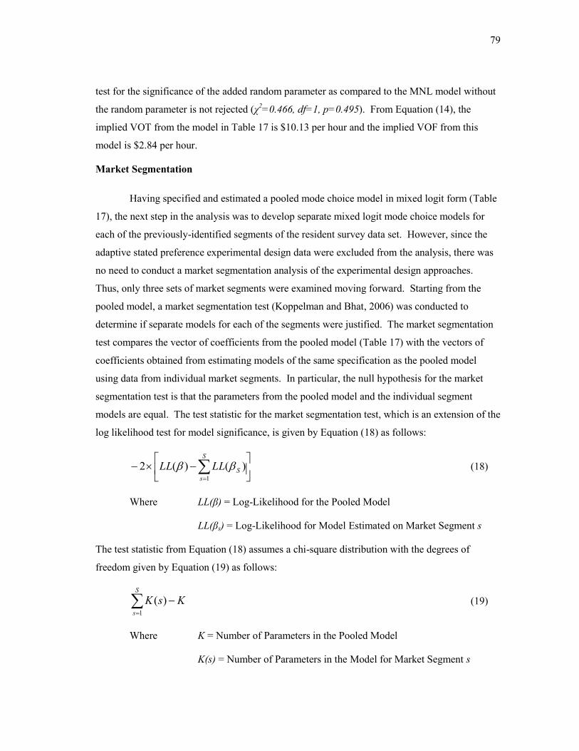
79
test for the significance of the added random parameter as compared to the MNL model without
the random parameter is not rejected (χ2=0.466, df=1, p=0.495). From Equation (14), the
implied VOT from the model in Table 17 is $10.13 per hour and the implied VOF from this
model is $2.84 per hour.
Market Segmentation
Having specified and estimated a pooled mode choice model in mixed logit form (Table
17), the next step in the analysis was to develop separate mixed logit mode choice models for
each of the previously-identified segments of the resident survey data set. However, since the
adaptive stated preference experimental design data were excluded from the analysis, there was
no need to conduct a market segmentation analysis of the experimental design approaches.
Thus, only three sets of market segments were examined moving forward. Starting from the
pooled model, a market segmentation test (Koppelman and Bhat, 2006) was conducted to
determine if separate models for each of the segments were justified. The market segmentation
test compares the vector of coefficients from the pooled model (Table 17) with the vectors of
coefficients obtained from estimating models of the same specification as the pooled model
using data from individual market segments. In particular, the null hypothesis for the market
segmentation test is that the parameters from the pooled model and the individual segment
models are equal. The test statistic for the market segmentation test, which is an extension of the
log likelihood test for model significance, is given by Equation (18) as follows:
S
s
SLLLL1
)()(2 (18)
Where LL(β) = Log-Likelihood for the Pooled Model
LL(βs) = Log-Likelihood for Model Estimated on Market Segment s
The test statistic from Equation (18) assumes a chi-square distribution with the degrees of
freedom given by Equation (19) as follows:
S
s
KsK1
)( (19)
Where K = Number of Parameters in the Pooled Model
K(s) = Number of Parameters in the Model for Market Segment s

80
If the test statistic given by Equation (18) is greater than the corresponding critical value from
the chi-square distribution with the degrees of freedom given by Equation (19), the market
segmentation test is rejected with the conclusion that the model parameters for the individual
market segment models are significantly different than the parameters of the pooled model and
thus the development of separate models for each market segment is justified. Note that the
market segmentation test is similar to the ANOVA test for the equality of means in that the test
examines the equality of the vectors of model coefficients; in some cases, certain coefficients
may be similar across market segments but the test can still be rejected if other coefficients are
sufficiently different from the pooled model.
The results of the market segmentation test for each of the three sets of market segments
previously identified are given in Table 18. For all three sets of market segments, the market
segmentation test comparing the pooled model with the individual segment models was rejected
(p<0.001 in all cases) and the estimation of separate models for each market segment is justified.
It is noted that in many cases, variables that are significant in the pooled ML model were found
to be not significant in the individual segment models.
Table 18: Market Segmentation Analysis
Market Segmentation Test χ2 Statistic DF P-Value
City: Waco or Temple 76.3 13 < 0.001
Visualization Package: Text-Only or Images 76.2 13 < 0.001
Visualization Package: Three Image Packages 177.7 26 < 0.001
Model coefficients for each of the three market segmentation tests can be found in
Appendix J. The following sections of this chapter provide more detailed analysis of each
market segment based on the optimal ML model for each segment.
COMMUNITY ANALYSIS
Mode choice models were estimated separately for the two study communities of Waco
and Temple using only data from residents from the individual community. The ML model
parameter estimates for each of the two study communities are given in Table 19. Examining
the models presented in Table 19, the Temple residents model is a better fit (adjusted ρc2=0.361)

81
than the Waco residents model (0.238). The number of respondents choosing rail was slightly
higher among Waco residents than Temple residents (50.1 percent versus 46.4 percent).
Table 19: Final ML Model Parameter Estimates by Study Community
Model Variables Waco
Model
Temple
Model
Travel Mode Variables
Travel Time (Minutes) -0.036 (-5.0) -0.017 (-4.5)
Travel Cost ($) -0.085 (-6.1) -0.074 (-10.5)
Rail: Service Headway (Hours) -0.227 (-6.3) -0.172 (-7.2)
Rail: Alternative-Specific Constant -- 0.872 (3.4)
Individual Traveler Dummy Variables
Auto: Age 18-24 0.665 (3.8) --
Auto: 4+ Household Vehicles -- 0.847 (3.1)
Auto: One Child in Household 0.838 (3.4) 0.709 (3.5)
Rail: Income $25,000 to $49,999 0.404 (2.5) --
Rail: One Household Vehicle 0.603 (3.9) --
Rail: Some College/Associate’s Degree -- 0.321 (2.0)
Rail: No Children in Household 0.566 (2.9) --
Factor Analysis Variables
Rail: Rail Travel Factor 0.338 (2.6) 0.292 (2.6)
Rail: Rail Community Impacts Factor 0.745 (4.7) 1.184 (9.9)
Rail: Intercity Rail Experience Factor -- 0.175 (2.5)
Standard Deviation of Random Parameters
Travel Time (Minutes) 0.071 (2.2) <0.001 (<0.1)
Model Fit Summary
Log-Likelihood (Constants Only) -1162.034 -956.574
Log-Likelihood (Model) -874.694 -600.749
Adjusted ρc2 0.238 0.361
D-Error (%) 0.296 0.279
A-Error (%) 2.035 2.162
Respondents Choosing Rail (%) 50.1 46.4
Choice Correctly Predicted (%) 62.0 66.7
Value of Time (per Hour) $25.41 $13.78
Value of Rail Headway (per Hour) $2.67 $2.32
Number of Observations 1,613 1,281
Note: T-ratio of parameter estimate given in parenthesis.
-- Indicates variable not significant at α=0.05 and removed from estimate.
Comparing the two models’ parameters, the travel mode variable parameters in the
Waco model are greater in magnitude than the Temple model. The travel time parameter in the

82
Waco model is twice the magnitude of the travel time parameter in the Temple model. The
magnitude of the rail service headway parameter for the Waco model was 33 percent larger than
the Temple model. This indicates that an improvement in the rail service headway (i.e. fewer
hours between services) increases the (relative) utility of rail for Temple residents more than a
similar improvement for Waco residents. The rail alternative-specific constant is significant in
the Temple model but not in the Waco model, reflecting a stronger preference for rail among
Temple residents if all other variables are equal. However, the rail alternative-specific constant
was not significant in the Waco model, implying an equal proportion of travelers selecting auto
or rail, ceteris paribus.
One variable that was not significant in the pooled model but was significant in the
Temple community model was the 4+ household vehicles dummy variable for the auto choice
model. Temple residents from households with four or more vehicles selected auto in the stated
preference questions 68 percent of the time, while Temple residents from households with less
than four vehicles selected auto only 48 percent of the time. It is not surprising that this dummy
variable is significant, as respondents from households with a larger number of vehicles would
likely demonstrate preferences for choosing automobile for trips out of town. However, the
proportion of Waco residents choosing auto in the stated preference questions did not vary
between residents from households with four or more vehicles and residents from households
with less than four vehicles, resulting in the variable not being significant in the Waco model.
The individual traveler dummy variable for “One Child in Household” was significant in
the automobile choice model for both communities and was the highest parameter estimate for
the Waco model (β=0.838). Among respondents from one-child households, automobile was
chosen 64 percent of the time (Waco) and 60 percent of the time (Temple), as compared with all
other respondents from both communities selecting automobile less than 50 percent of the time.
Among Waco residents, the rail choice model contained three significant individual
traveler dummy variables: annual household income between $25,000 and $49,999, one
household vehicle, and no children in household. The contributions of the latter two variables to
the (relative) utility of rail travel among Waco residents were approximately equal and slightly
greater than the contribution of the first variable. Waco residents that were classified in one or
more of these three categories selected rail in the stated preference questions between 56 and 58
percent of the time, while residents that were not classified into one or more of these three
83
categories selected rail in the stated preference questions between 47 and 51 percent of the time.
The only individual traveler dummy variable that was significant in the rail choice model for
Temple residents was the “Some College or Associate’s Degree” educational attainment dummy
variable. Temple residents reporting “Some College or Associate’s Degree” as their highest
level of education chose rail in the stated preference questions 57 percent of the time, as opposed
to Temple residents with other levels of educational attainment choosing rail in the stated
preference questions only 48 percent of the time.
The highest parameter estimate in the Temple model was the rail community impacts
factor variable in the rail choice model (β=1.184), implying a strong relationship between
Temple residents’ views on the impacts of new rail service on the community and the likelihood
of choosing rail in the stated preference questions. The rail community impacts factor variable
was also significant in the Waco model, although it was smaller in magnitude. The finding that
the parameter estimate for the rail community impacts factor variable is higher for Temple
residents suggests that the contribution of residents’ beliefs on the positive impacts of new rail
service on the community to the estimated likelihood of choosing rail is greater in communities
where new intercity passenger rail service would be incremental change in rail service (i.e.
would replace existing Amtrak service) than for communities where new rail service would be
established where none currently exists. The intercity rail experience factor variable in the rail
choice model was also significant for Temple residents. The significance of this variable in the
Temple model but not in the Waco model could be attributed to fact that residents of Temple
have more experience with rail transportation due to the Amtrak Texas Eagle route serving the
community at the time of the survey (see Table 4). The standard deviation of the random
parameter is significant in the Waco model (p=0.027) but not in the Temple model (p=0.998).
From the models presented in Table 19, the implied VOT for Waco residents is $25.41 per hour,
higher than the implied VOT for Temple residents estimated at $13.78 per hour. The implied
VOF from the models followed a similar pattern, with the VOF for Waco residents estimated at
$2.67 per hour and for Temple residents estimated at $2.32 per hour.
VISUALIZATION ANALYSIS
In the survey, respondents were randomly-assigned to one of three image packages: a
text-only description of a proposed passenger rail service, an image of a “typical” intercity

84
passenger train (see Figure 3), or an image of a “flashy” intercity passenger train (see Figure 4).
Two sets of mode choice models were developed examining the differences among respondents
viewing different image packages. The first set of models compare the text-only survey version
with the survey version containing both image packages combined (see Table 20). The second
set of models compare the three image packages separately (see Table 21).
Table 20: Final ML Model Parameter Estimates by Text-Only and Image Packages
Model Variables Text-Only
Model
Photos
Model
Travel Mode Variables
Travel Time (Minutes) -0.029 (-4.6) -0.009 (-2.8)
Travel Cost ($) -0.103 (-6.6) -0.072 (-12.2)
Rail: Service Headway (Hours) -0.168 (-4.6) -0.236 (-13.3)
Rail: Alternative-Specific Constant -- 1.587 (8.3)
Individual Traveler Dummy Variables
Auto: Age 18-24 -- 0.721 (5.1)
Auto: One Child in Household -- 1.211 (7.7)
Rail: Income $25,000 to $49,999 0.482 (2.2) 0.330 (2.6)
Rail: Age 65 or Older 1.323 (3.2) --
Rail: One Household Vehicle -- 0.386 (3.2)
Rail: One Adult in Household 0.550 (2.3) --
Factor Analysis Variables
Rail: Rail Travel Factor 0.850 (4.2) --
Rail: Rail Community Impacts Factor 0.713 (3.8) 1.096 (15.9)
Rail: Intercity Rail Experience Factor 0.459 (4.2) --
Standard Deviation of Random Parameters
Travel Time (Minutes) 0.060 (2.5) 0.001 (<0.1)
Model Fit Summary
Log-Likelihood (Constants Only) -697.350 -1422.157
Log-Likelihood (Model) -449.116 -1024.634
Adjusted ρc2 0.343 0.273
D-Error (%) 0.351 0.151
A-Error (%) 3.749 1.173
Respondents Choosing Rail (%) 48.0 48.6
Choice Correctly Predicted (%) 65.2 64.5
Value of Time (per Hour) $16.89 $7.50
Value of Rail Headway (per Hour) $1.63 $3.28
Number of Observations 943 1,991
Note: T-ratio of parameter estimate given in parenthesis.
-- Indicates variable not significant at α=0.05 and removed from estimate.
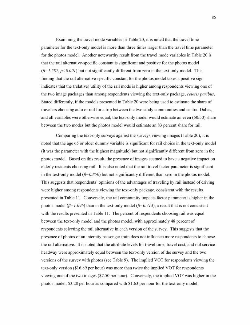
85
Examining the travel mode variables in Table 20, it is noted that the travel time
parameter for the text-only model is more than three times larger than the travel time parameter
for the photos model. Another noteworthy result from the travel mode variables in Table 20 is
that the rail alternative-specific constant is significant and positive for the photos model
(β=1.587, p<0.001) but not significantly different from zero in the text-only model. This
finding that the rail alternative-specific constant for the photos model takes a positive sign
indicates that the (relative) utility of the rail mode is higher among respondents viewing one of
the two image packages than among respondents viewing the text-only package, ceteris paribus.
Stated differently, if the models presented in Table 20 were being used to estimate the share of
travelers choosing auto or rail for a trip between the two study communities and central Dallas,
and all variables were otherwise equal, the text-only model would estimate an even (50/50) share
between the two modes but the photos model would estimate an 83 percent share for rail.
Comparing the text-only surveys against the surveys viewing images (Table 20), it is
noted that the age 65 or older dummy variable is significant for rail choice in the text-only model
(it was the parameter with the highest magnitude) but not significantly different from zero in the
photos model. Based on this result, the presence of images seemed to have a negative impact on
elderly residents choosing rail. It is also noted that the rail travel factor parameter is significant
in the text-only model (β=0.850) but not significantly different than zero in the photos model.
This suggests that respondents’ opinions of the advantages of traveling by rail instead of driving
were higher among respondents viewing the text-only package, consistent with the results
presented in Table 11. Conversely, the rail community impacts factor parameter is higher in the
photos model (β=1.096) than in the text-only model (β=0.713), a result that is not consistent
with the results presented in Table 11. The percent of respondents choosing rail was equal
between the text-only model and the photos model, with approximately 48 percent of
respondents selecting the rail alternative in each version of the survey. This suggests that the
presence of photos of an intercity passenger train does not influence more respondents to choose
the rail alternative. It is noted that the attribute levels for travel time, travel cost, and rail service
headway were approximately equal between the text-only version of the survey and the two
versions of the survey with photos (see Table 9). The implied VOT for respondents viewing the
text-only version ($16.89 per hour) was more than twice the implied VOT for respondents
viewing one of the two images ($7.50 per hour). Conversely, the implied VOF was higher in the
photos model, $3.28 per hour as compared with $1.63 per hour for the text-only model.

86
Table 21: Final ML Model Parameter Estimates by Three Image Packages
Model Variables Text-Only
Model
Typical
Model
Flashy
Model
Travel Mode Variables
Travel Time (Minutes) -0.029 (-4.6) -0.014 (-2.4) -0.013 (-2.6)
Travel Cost ($) -0.103 (-6.6) -0.050 (-4.6) -0.104 (-11.4)
Rail: Service Headway (Hours) -0.168 (-4.6) -0.259 (-6.4) -0.274 (-10.5)
Rail: Alternative-Specific Constant -- 1.265 (3.8) 1.692 (6.1)
Individual Traveler Dummy Variables
Auto: Age 18-24 -- 1.364 (4.9) --
Auto: One Child in Household -- 1.784 (5.4) --
Rail: Income $25,000 to $49,999 0.482 (2.2) 0.864 (3.7) --
Rail: Age 65 or Older 1.323 (3.2) -- --
Rail: One Household Vehicle -- 0.941 (4.2) --
Rail: Some College/Associate’s Degree -- -- 0.428 (2.4)
Rail: One Adult in Household 0.550 (2.3) -- 0.360 (2.2)
Factor Analysis Variables
Rail: Rail Travel Factor 0.850 (4.2) -- --
Rail: Rail Community Impacts Factor 0.714 (3.8) 1.297 (7.3) 1.280 (11.9)
Rail: Intercity Rail Experience Factor 0.459 (4.2) -- --
Standard Deviation of Random Parameters
Travel Time (Minutes) 0.060 (2.5) 0.036 (1.2) <0.001 (<0.1)
Model Fit Summary
Log-Likelihood (Constants Only) -697.350 -697.605 -724.529
Log-Likelihood (Model) -449.116 -468.104 -493.339
Adjusted ρc2 0.343 0.316 0.309
D-Error (%) 0.351 0.382 0.157
A-Error (%) 3.749 4.362 1.892
Respondents Choosing Rail (%) 48.0 48.8 48.6
Choice Correctly Predicted (%) 65.2 65.2 66.5
Value of Time (per Hour) $16.89 $16.80 $7.50
Value of Rail Headway (per Hour) $1.63 $5.18 $2.63
Number of Observations 943 983 1,000
Note: T-ratio of parameter estimate given in parenthesis.
-- Indicates variable not significant at α=0.05 and removed from estimate.
Comparing the model parameters for the two image packages (Table 21), it is noted that
the magnitude of the travel cost parameter for the flashy image model is more than two times
greater than the travel cost parameter for the typical image model. The travel time and rail
service headway parameters are approximately equal between the two image packages, implying
that the quality of the train equipment portrayed in the photo does not influence the contribution
of the rail service headway to the (relative) utility of the rail mode. However, the rail

87
alternative-specific constant was higher for the flashy image model (β=1.692) than for the
typical image model (β=1.265). Assuming all other variables in the model are equal, the
(relative) utility of the rail mode is higher among respondents viewing the flashy image model
than among respondents viewing the typical image model. This finding was consistent with a
priori expectations on how respondents might react to the two different photo packages.
Examining the typical image package model parameters, the one child in household
variable for the auto choice model was the highest among all the individual traveler dummy
variables (β=1.784). One possible explanation for the strong preference for auto among
respondents from one-child households that viewed the typical image package could be that the
respondent did not find the “typical” train equipment presented in the image (see Figure 3)
appealing or otherwise suitable for traveling with a child. This explanation is supported by the
average score for the opinion item “Traveling on Intercity Passenger Rail Would be More
Enjoyable than Driving” among respondents from one-child households that viewed the typical
image package, calculated as 5.07/7. This score was lower than the average score on this item
for all respondents viewing the typical image package (5.38/7, see Table 12). Examining the
parameters for the flashy image model, it is noted that travel time and travel cost are the only
significant variables in the auto mode choice model; none of the individual traveler dummy
variables were found to be significant.
The model parameters for the rail community impacts factor in Table 21 are
approximately equal between the typical image model and the flashy image model. This means
that the quality of the train equipment shown in the images presented prior to the stated
preference questions does not affect how this variable influences the (relative) utility of the rail
option in the travel mode choice model. The similarity between the typical image model and the
flashy image model is also reflected in the percent of respondents choosing rail in the stated
preference questions, which is approximately equal between the two models. However, due to
the magnitude differences in the travel cost parameter between the typical and flashy image
models, the implied VOT and VOF estimates for these models are also different. Specifically,
the implied VOT and VOF are higher for the model drawn from respondents viewing the typical
image package than for the flashy image package. The implied VOT from the typical image
model is $16.80 per hour. This was approximately equal to the implied VOT from the text-only
model, and more than twice as much as the implied VOT from the flashy image model, $7.50 per

88
hour. A similar pattern is realized with the implied VOF, which is $5.18 per hour for the typical
image model and $2.63 per hour for the flashy image model. This is not consistent with the a
priori expectation that residents would have a higher valuation of traveling on equipment that is
portrayed as more modern and flashy.
VALUE OF TIME ANALYSIS
Having presented a series of travel mode choice models for the specific segments, the
final portion of this analysis focuses on the implied VOT from these models. As Roth (1998)
argues, an individual traveler’s value of time could be considered the most important factor in
determining his or her choice of modes for a particular trip because it represents the trade-off an
individual is willing or able to make between travel time and travel cost. VOT is also used as an
input to travel demand models for proposed high-speed intercity passenger rail services
(Transportation Economics and Management Systems, Inc., 2008; 2010). Furthermore, traveler
VOT is a key component in the assessment of traveler costs in benefit-cost analyses or other
economic appraisals of proposed or existing high-speed intercity passenger rail projects (e.g.
Brand et al., 2001; De Rus and Inglada, 1997; Economic Development Research Group and
AECOM, 2011; Federal Railroad Administration, 1997; Levinson and Gillen, 1998; Shearin,
1997). The capital costs for new high-speed intercity passenger rail investments are very large,
with typical estimated costs between $7 and $35 million per mile (Peterman et al., 2009).
Therefore, accurate economic appraisals for proposed projects are critical to ensure informed
decision-making and responsible use of scarce public resources for transportation infrastructure
projects. The survey conducted in this dissertation offers an ideal setting in which to evaluate
the effects of community type and the visualization of travel alternatives in a stated preference
survey on the travelers’ estimated value of time.
The implied VOT for each of the mode choice models presented in this chapter was
estimated using Equation (14) and presented with each model estimate. While valid, the use of
Equation (14) to estimate VOT in this application does not make use of all the information
available. Specifically, the use of Equation (14) ignores the fact that the models presented in this
chapter are estimated in mixed logit form and that the travel time parameter (βTT) has a random
(in this case, triangular) distribution. Consequently, a more accurate estimation of VOT can be
obtained via simulation (Armstrong et al., 2001; Espino et al., 2006; Hensher and Greene, 2003;

89
Rizzi et al., 2011; Sillano and Ortúzar, 2005). The VOT simulation analysis was conducted for
each model segment using the JMP statistical analysis software program (SAS Institute Inc.,
2010). A draw of 100,000 random numbers from the uniform distribution U (0,1) was obtained
and converted to the triangular distribution using Equation (15). These values for t and the
estimated travel time parameter (βTT) from each individual segment were used to calculate an
individual-specific travel time parameter estimate using Equation (17). Using this estimate and
the travel cost parameter estimate from each model segment, the resulting VOT was calculated
using Equation (14). From this set of 100,000 VOT estimates, a random draw of 1,000 values
was obtained and the mean VOT estimated. This process was repeated 10,000 times to estimate
the mean and standard deviation of the underlying distribution of the VOT. It is noted that a
single draw of the VOT (n=1,000) assumes a triangular distribution but the distribution of the
mean VOT estimates (n=10,000) assumes a normal distribution on the basis of the central limit
theorem. Consequently, a 95 percent confidence interval around the mean VOT value for each
market segment was obtained by identifying the 0.025 and 0.975 percentile values from the VOT
distribution for each market segment (Armstrong et al., 2001; Espino et al., 2006; Hensher and
Greene, 2003). The mean VOT, its standard deviation, and the 95 percent confidence interval
around the mean VOT for the pooled model and each market segment are displayed in Table 22.
Table 22: Value of Time Analysis by Market Segment (Dollars per Hour)
Market Segment Mean VOT VOT Standard
Deviation
95% Confidence
Interval Bounds
Pooled Model (Table 17) $9.91 $0.127 (9.65, 10.16)
Waco Residents (Table 19) $25.61 $0.328 (24.96, 26.25)
Temple Residents (Table 19) $13.84 $0.177 (13.50, 14.20)
Text-Only Package (Table 20) $16.90 $0.218 (16.47, 17.33)
Both Image Packages (Table 20) $7.79 $0.101 (7.59, 7.99)
Typical Image Package (Table 21) $16.57 $0.212 (16.16, 16.98)
Flashy Image Package (Table 21) $7.40 $0.095 (7.22, 7.59)
The VOT for the pooled model presented in Table 22, $9.91 per hour is slightly lower,
but still on the same order of magnitude as the VOT that was estimated for automobile travelers
making personal trips in recent high-speed intercity passenger rail feasibility studies (Outwater et
al., 2010; Transportation Economics and Management Systems, Inc., 2008; 2010). Examining
the VOT of residents in the two study communities, the mean VOT for Waco residents is $25.61
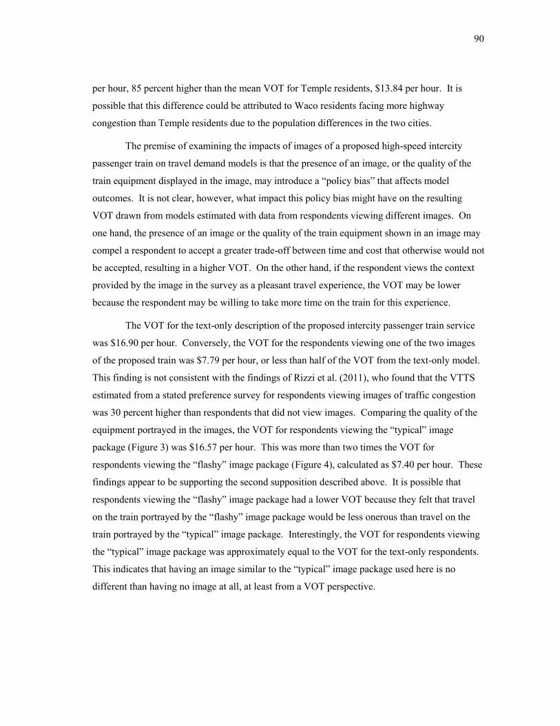
90
per hour, 85 percent higher than the mean VOT for Temple residents, $13.84 per hour. It is
possible that this difference could be attributed to Waco residents facing more highway
congestion than Temple residents due to the population differences in the two cities.
The premise of examining the impacts of images of a proposed high-speed intercity
passenger train on travel demand models is that the presence of an image, or the quality of the
train equipment displayed in the image, may introduce a “policy bias” that affects model
outcomes. It is not clear, however, what impact this policy bias might have on the resulting
VOT drawn from models estimated with data from respondents viewing different images. On
one hand, the presence of an image or the quality of the train equipment shown in an image may
compel a respondent to accept a greater trade-off between time and cost that otherwise would not
be accepted, resulting in a higher VOT. On the other hand, if the respondent views the context
provided by the image in the survey as a pleasant travel experience, the VOT may be lower
because the respondent may be willing to take more time on the train for this experience.
The VOT for the text-only description of the proposed intercity passenger train service
was $16.90 per hour. Conversely, the VOT for the respondents viewing one of the two images
of the proposed train was $7.79 per hour, or less than half of the VOT from the text-only model.
This finding is not consistent with the findings of Rizzi et al. (2011), who found that the VTTS
estimated from a stated preference survey for respondents viewing images of traffic congestion
was 30 percent higher than respondents that did not view images. Comparing the quality of the
equipment portrayed in the images, the VOT for respondents viewing the “typical” image
package (Figure 3) was $16.57 per hour. This was more than two times the VOT for
respondents viewing the “flashy” image package (Figure 4), calculated as $7.40 per hour. These
findings appear to be supporting the second supposition described above. It is possible that
respondents viewing the “flashy” image package had a lower VOT because they felt that travel
on the train portrayed by the “flashy” image package would be less onerous than travel on the
train portrayed by the “typical” image package. Interestingly, the VOT for respondents viewing
the “typical” image package was approximately equal to the VOT for the text-only respondents.
This indicates that having an image similar to the “typical” image package used here is no
different than having no image at all, at least from a VOT perspective.

91
CHAPTER VI
CONCLUSIONS AND RECOMMENDATIONS
High-speed passenger rail is viewed by many in the U.S transportation planning and
policy communities as an ideal solution for fast, safe, and resource-efficient mobility in high-
demand intercity corridors. Recent policy and regulatory directions by the U.S. government
have signaled a new role for high-speed intercity passenger rail in the national transportation
system. Moving forward, there is a need to improve upon the tools used by transportation
planners to estimate demand for new high-speed intercity passenger rail systems. Consequently,
the overall goal of this dissertation was to gain a better understanding of the demand for high-
speed intercity passenger rail services in small- or medium-sized intermediate communities and
improve planners’ ability to estimate such demand through surveys of travelers. In pursuit of
this goal, an Internet-based survey questionnaire was distributed to residents of two communities
located along the federally-designated South Central High-Speed Rail Corridor in Central Texas.
A total of 1,160 surveys were obtained from residents, yielding valuable information about
resident travel behavior, decision-making, and demographics. Mixed logit travel mode choice
models constructed from stated preference data obtained in the resident survey yielded additional
insight toward the goals of this dissertation.
SUMMARY OF FINDINGS
Analysis of the resident survey data obtained in this dissertation revealed several
interesting findings relevant to better understanding the demand for high-speed intercity
passenger rail in small- or medium-sized intermediate communities, experimental designs for
stated preference surveys, and the visualization of travel alternatives in stated preference
surveys. The most relevant findings are summarized in the following sections.
Intermediate Communities
The geographic focus of this dissertation was small- or medium-sized communities
located in an intermediate area between major large urban areas of an intercity corridor which
has been proposed for high-speed passenger rail service. Specifically, residents of the Central
Texas communities of Waco (population 124,805) and Temple (population 66,102) were
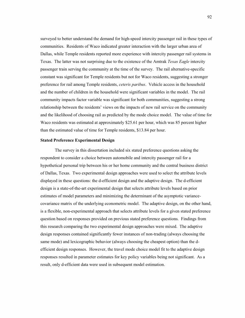
92
surveyed to better understand the demand for high-speed intercity passenger rail in these types of
communities. Residents of Waco indicated greater interaction with the larger urban area of
Dallas, while Temple residents reported more experience with intercity passenger rail systems in
Texas. The latter was not surprising due to the existence of the Amtrak Texas Eagle intercity
passenger train serving the community at the time of the survey. The rail alternative-specific
constant was significant for Temple residents but not for Waco residents, suggesting a stronger
preference for rail among Temple residents, ceteris paribus. Vehicle access in the household
and the number of children in the household were significant variables in the model. The rail
community impacts factor variable was significant for both communities, suggesting a strong
relationship between the residents’ views on the impacts of new rail service on the community
and the likelihood of choosing rail as predicted by the mode choice model. The value of time for
Waco residents was estimated at approximately $25.61 per hour, which was 85 percent higher
than the estimated value of time for Temple residents, $13.84 per hour.
Stated Preference Experimental Design
The survey in this dissertation included six stated preference questions asking the
respondent to consider a choice between automobile and intercity passenger rail for a
hypothetical personal trip between his or her home community and the central business district
of Dallas, Texas. Two experimental design approaches were used to select the attribute levels
displayed in these questions: the d-efficient design and the adaptive design. The d-efficient
design is a state-of-the-art experimental design that selects attribute levels based on prior
estimates of model parameters and minimizing the determinant of the asymptotic variance-
covariance matrix of the underlying econometric model. The adaptive design, on the other hand,
is a flexible, non-experimental approach that selects attribute levels for a given stated preference
question based on responses provided on previous stated preference questions. Findings from
this research comparing the two experimental design approaches were mixed. The adaptive
design responses contained significantly fewer instances of non-trading (always choosing the
same mode) and lexicographic behavior (always choosing the cheapest option) than the d-
efficient design responses. However, the travel mode choice model fit to the adaptive design
responses resulted in parameter estimates for key policy variables being not significant. As a
result, only d-efficient data were used in subsequent model estimation.
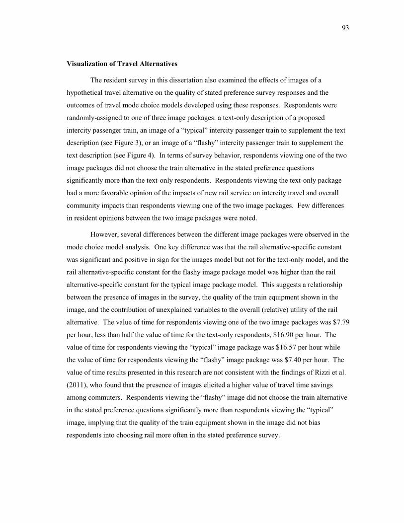
93
Visualization of Travel Alternatives
The resident survey in this dissertation also examined the effects of images of a
hypothetical travel alternative on the quality of stated preference survey responses and the
outcomes of travel mode choice models developed using these responses. Respondents were
randomly-assigned to one of three image packages: a text-only description of a proposed
intercity passenger train, an image of a “typical” intercity passenger train to supplement the text
description (see Figure 3), or an image of a “flashy” intercity passenger train to supplement the
text description (see Figure 4). In terms of survey behavior, respondents viewing one of the two
image packages did not choose the train alternative in the stated preference questions
significantly more than the text-only respondents. Respondents viewing the text-only package
had a more favorable opinion of the impacts of new rail service on intercity travel and overall
community impacts than respondents viewing one of the two image packages. Few differences
in resident opinions between the two image packages were noted.
However, several differences between the different image packages were observed in the
mode choice model analysis. One key difference was that the rail alternative-specific constant
was significant and positive in sign for the images model but not for the text-only model, and the
rail alternative-specific constant for the flashy image package model was higher than the rail
alternative-specific constant for the typical image package model. This suggests a relationship
between the presence of images in the survey, the quality of the train equipment shown in the
image, and the contribution of unexplained variables to the overall (relative) utility of the rail
alternative. The value of time for respondents viewing one of the two image packages was $7.79
per hour, less than half the value of time for the text-only respondents, $16.90 per hour. The
value of time for respondents viewing the “typical” image package was $16.57 per hour while
the value of time for respondents viewing the “flashy” image package was $7.40 per hour. The
value of time results presented in this research are not consistent with the findings of Rizzi et al.
(2011), who found that the presence of images elicited a higher value of travel time savings
among commuters. Respondents viewing the “flashy” image did not choose the train alternative
in the stated preference questions significantly more than respondents viewing the “typical”
image, implying that the quality of the train equipment shown in the image did not bias
respondents into choosing rail more often in the stated preference survey.

94
RECOMMENDATIONS
Based on the findings from this dissertation, several recommendations for high-speed
intercity passenger rail planning and the design of traveler surveys for rail planning activities are
provided. First, regarding the treatment of small- or medium-sized intermediate communities in
demand estimates for proposed high-speed intercity passenger rail lines, this research indicated
differences in values of time and rail service headway between residents of the two study
communities, Waco and Temple. Consequently, demand estimates for new high-speed intercity
passenger rail lines that are planned to serve intermediate communities should not assume that
residents of all intermediate communities have similar travel preferences or values of travel time
and rail service headway. These findings also revive a classic policy debate in transportation:
can new investment in intercity passenger rail service be designed such that a balance between
serving the mobility needs of those traveling between major urban areas and providing
intermediate community residents with access to these rail systems be struck? While this
research does not completely answer this question, the traveler valuations presented here can
assist with the economic appraisal of alternative investments to serve intermediate communities
with rail systems and support informed decision-making on infrastructure planning.
Second, with respect to stated preference experimental designs for high-speed intercity
passenger rail planning, this dissertation showed that the d-efficient design produced a better-
quality travel mode choice model than the adaptive design. Therefore, it is recommended that
the d-efficient experimental design be used by rail planners in future stated preference surveys
for high-speed intercity passenger rail ridership estimates. Finally, regarding the use of images
showing hypothetical travel alternatives in a stated preference survey, this dissertation found
value of time differences among respondents that viewed the different image packages.
However, no difference in the percentage of respondents selecting rail in the stated preference
questions was noted among respondents viewing the different images. In light of these findings,
it is recommended that images be used to improve realism in stated preference surveys for high-
speed intercity passenger rail planning, particularly where no rail services currently exist and
travelers may be unfamiliar with rail transportation or the use of images to support respondent
decision-making may be otherwise justified. However, if images are used, every effort should
be made to make the images as realistic as possible in terms of portraying the type of equipment
95
to be used on a proposed rail line in order to elicit the most accurate mode choice model
parameters and the resulting traveler valuations.
FUTURE RESEARCH
Given the revived interest in high-speed and other forms of intercity passenger rail
among planners, policymakers, and the general public, future research opportunities on
increasing the accuracy of ridership estimates for new intercity passenger rail lines and
improving traveler surveys used for intercity passenger rail planning activities are abundant.
Future research could also address some of the limitations that are inherent in the present study.
Regarding demand estimates for intermediate communities, the results of this dissertation are
limited to respondents of an Internet-based survey of residents of two communities in Central
Texas. More surveys of residents in different communities located along the South Central
High-Speed Rail Corridor other Federally-designated high-speed rail corridors would help form
a better understanding of the travel behavior of residents in these communities and also confirm
the stability of the travel mode choice model parameters. The use of a resident survey (rather
than a survey intercepting travelers during an intercity trip) may also allow for an estimate of
latent or induced travel demand resulting from new rail services that would otherwise be missed
with other survey approaches. While the use of the Internet in this survey provided key benefits
to the research, limitations on the generalizability of the research findings stemming from the use
of the Internet (some of which were accounted for in the sample weights) could be overcome
with a more robust (i.e. probability-based) sampling approach. Also, while surveys with
controversial or compelling subjects will always be affected by some degree of respondent self-
selection, a more robust sampling plan should overcome some of those issues as well. Another
limitation of this work is that the stated preference responses were based on a purely
hypothetical proposed intercity passenger rail system and a hypothetical trip made by the
respondent between their home community and central Dallas. If an actual improved rail system
is proposed in the South Central High-Speed Rail Corridor, a new survey of intermediate
community residents with travel time, travel cost, and rail service headway levels that more
closely resemble the proposed system would be desired and yield more accurate results.
Specific to the design of traveler surveys for high-speed intercity passenger rail
planning, the use of the d-efficient stated preference experimental design should continue to be
96
examined, particularly in light of the limited use of this state-of-the-art experimental design in
this application to date. Refinements to the adaptive stated preference technique may lead to
greater stability in the resulting travel mode choice models. More attributes could be added to
the stated preference experiment in order to more accurately assess traveler valuations of in-
vehicle versus out-of-vehicle time or other issues related to rail station accessibility. Perhaps the
area that holds the most promise for future research is the effects of images or other multimedia
on stated preference responses. Building upon the limited amount of existing research on this
topic, advances in survey deployment technology and increasing computing power in personal
devices should allow for plentiful opportunities for future research in this area. Beyond
comparing the travel mode choice models built using data from different types of images, future
surveys could also include a set of questions specifically evaluating how the respondent reacted
to the presence of images. Regardless, the goal of future research in this area should be to better
understand the potential limitations and biases associated with ridership estimates for high-speed
intercity passenger rail projects and the methods used to develop such estimates, always bearing
in mind the main goal of transportation planning: supplying decision-makers with timely and
accurate information with which to make decisions on the allocation of scarce public resources
for transportation infrastructure investment.

97
REFERENCES
Adler, T., Rimmer, L., Carpenter, D., 2002. Use of Internet-Based Household Travel Diary
Survey Instrument. Transportation Research Record 1804, 134-143.
AECOM Consulting, Wilbur Smith Associates, 2002. Investment Grade Ridership Study
Summary Report. Prepared for Florida High-Speed Rail Authority.
<http://www.floridabullettrain.com/fhsra/uploaddocuments/p25/Ridership%20Study%20-
%20all%20reports.pdf>. Accessed 10 January 2012.
Alsnih, R., 2006. Characteristics of Web Based Surveys and Applications in Travel Research.
In: Stopher, P., Stecher, C. (Eds.), Travel Survey Methods: Quality and Future Directions,
Elsevier, Oxford, United Kingdom.
Amtrak Government Affairs, 2010. Amtrak Fact Sheet, Fiscal Year 2010, State of Texas.
Amtrak Government Affairs, Washington, D.C. <http://www.amtrak.com/pdf/
factsheets/TEXAS10.pdf>. Accessed 27 November 2011.
Anderson, D.A., Louviere, J.J., Daniel, T., Orland, B., 1993. Comparing Verbal and Visual
Attribute Representations in Choice-Based Conjoint: Videotapes Versus Paper and Pencil.
Working Paper, Department of Marketing, University of Utah, Salt Lake City.
Arentze, T., Borgers, A., Timmermans, H., DelMistro, R., 2003. Transport Stated Choice
Responses: Effects of Task Complexity, Presentation Format, and Literacy. Transportation
Research Part E 39, 229-244.
Armstrong, P., Garrido, R., Ortúzar, J., 2001. Confidence Intervals to Bound the Value of Time.
Transportation Research Part E 37, 143-161.
Bhat, C.R., 1995. A Heteroscedastic Extreme Value Model of Intercity Travel Mode Choice.
Transportation Research Part B 29 (6), 471-483.
Bhat, C.R., 1997. An Endogenous Segmentation Mode Choice Model with an Application to
Intercity Travel. Transportation Science 31 (1), 34-48.
Bhat, C.R., 2001. Quasi-Random Maximum Simulated Likelihood Estimation of the Mixed
Multinomial Logit Model. Transportation Research Part B 35, 677-693.
Bliemer, M.C.J., Rose, J.M., 2005. Efficiency and Sample Size Requirements for Stated Choice
Studies. Working Paper ILTS-WP-05-08, Institute of Transport and Logistics Studies,
Sydney, Australia. <http://ws.econ.usyd.edu.au/itls/wp-archive/itls_wp_05-08.pdf>.
Accessed 16 December 2010.
Bliemer, M.C.J., Rose, J.M., 2009. Designing Stated Choice Experiments: State of the Art. In:
Kitamura, R., Yoshii, T., Yamamoto, T., (Eds.), The Expanding Sphere of Travel Behavior
Research: Selected Papers from the 11th International Conference on Travel Behaviour
Research, International Association for Travel Behaviour Research, Emerald Press, Bingley,
United Kingdom.
Bliemer, M.C.J., Rose, J.M., 2011. Experimental Design Influences on Stated Choice Outputs:
An Empirical Study in Air Travel Choice. Transportation Research Part A 45, 63-79.
Blum, U., Haynes, K., Karlsson, C., 1997. Introduction to the Special Issue: The Regional and
Urban Effects of High-Speed Trains. Annals of Regional Science 31, 1-20.
98
Blume, L., Brandenburger, A., Dekel, E., 2006. An Overview of Lexicographic Choice Under
Uncertainty. Annals of Operations Research 19, 231-246.
Bonnafous, A., 1987. The Regional Impact of the TGV. Transportation 14 (2), 127-137.
Botimer, T.C., Chan, J., Mathieu, J-M., Kanafani, A., 1994. Forecasting Intercity Travel in
California: Design of a Survey to Estimate the Demand for High Speed Rail Transportation.
Research Report UCB-ITS-RR-94-10, Institute of Transportation Studies, University of
California, Berkeley.
Brackstone, G.J., Rao, J.N.K., 1976. Raking Ratio Estimators. Survey Methodology 2, 63-69.
Bradley, M., 1988. Realism and Adaptation in Designing Hypothetical Travel Choice Concepts.
Journal of Transport Economics and Policy 22 (1), 121-137.
Brand, D., Kiefer, M.R., Parody, T.E., Mehndiratta, S.R., 2001. Application of Benefit-Cost
Analysis to the Proposed California High-Speed Rail System. Transportation Research
Record 1742, 9-16.
Brand, D., Parody, T.E., Hsu, P.S., Tierney, K.F., 1992. Forecasting High-Speed Rail Ridership.
Transportation Research Record 1341, 12-18.
Brown, D., 2001. When Rural Communities Lose Passenger Rail Service. Rural Development
Perspectives 12 (2), 13-18.
Buckeye, K.R., 1992. Implications of High-Speed Rail on Air Traffic. Transportation Research
Record 1341, 19-27.
Calfee, J., Winston, C., Stempski, R., 2001. Econometric Issues in Estimating Consumer
Preferences from Stated Preference Data: A Case Study of the Value of Automobile Travel
Time. The Review of Economics and Statistics 83 (4), 699-707.
Cambridge Systematics, Inc., 2007. Accounting for Fuel Efficiency in Texas Fuel Tax Revenue
Estimations: Final Report. Prepared for the Texas Department of Transportation.
<http://www.camsys.com/pubs/TXDot_GBE.pdf>. Accessed 6 October 2011.
Cambridge Systematics, Inc., 2008. Desert Xpress Ridership Forecast Review. Prepared for
Circle Point. <http://www.fra.dot.gov/rpd/freight/1703.shtml>. Accessed 8 June 2009.
Cambridge Systematics, Inc., Citilabs, Corey, Canapary, & Galanis, HLB Decision Economics,
Inc., Mark Bradley Research & Consulting, Systra Consulting, Inc., 2005. Bay
Area/California High-Speed Rail Ridership and Revenue Forecasting Study: Model Design,
Data Collection, and Performance Measures. Prepared for the Metropolitan Transportation
Commission. <http://www.cahighspeedrail.ca.gov/WorkArea/DownloadAsset.aspx
?id=7934>. Accessed 16 December 2009.
Cambridge Systematics, Inc., Citilabs, Systra Consulting, Inc., 2006. Bay Area/California High-
Speed Rail Ridership and Revenue Forecasting Study: Levels-of-Service Assumptions and
Forecast Alternatives. Prepared for the Metropolitan Transportation Commission and the
California High-Speed Rail Authority. <http://www.cahighspeedrail.ca.gov/WorkArea/
DownloadAsset.aspx ?id=7923>. Accessed 11 February 2011.
Campos, J., de Rus, G., 2009. Some Stylized Facts About High-Speed Rail: A Review of HSR
Experiences Around the World. Transport Policy 16, 19-28.

99
Capon, P., Longo, G., Santorini, F., 2003. Rail Vs. Air Transport for Medium Range Trips. In:
Proceedings of ICTS 2003, Nova Gorica, Slovenia, 6-8 November.
Carlsson, F., 2003. The Demand for Intercity Public Transport: The Case of Business
Passengers. Applied Economics 35 (1), 41-50.
Carson, R.T., Louviere, J.J., Anderson, D.A., Arabie, P., Bunch, D.S., Hensher, D.A., Johnson,
R.M., Kuhfeld, W.F., Steinberg, D., Swait, J., Timmermans, H., Wiley, J.B., 1994.
Experimental Analysis of Choice. Marketing Letters 5 (4), 351-368.
Charles River Associates, 1993. Independent Ridership and Passenger Revenue Projections for
the Texas TGV Corporation High Speed Rail System in Texas. Submitted to the Texas TGV
Corporation.
Chen, C., Hall, P., 2011. The Impacts of High-Speed Trains on British Economic Geography: A
Study of the UK’s InterCity 125/225 and its Effects. Journal of Transport Geography 19 (4),
689-704.
ChoiceMetrics, 2010. Ngene 1.0.2 User Manual & Reference Guide. ChoiceMetrics Pty. Ltd.
<http://www.choice-metrics.com/documentation.html>. Accessed 21 December 2010.
Clark, C., 1958. Transport-Maker and Breaker of Cities. Town Planning Review 28 (4), 237-250.
Corey, Canapary, & Galanis Research, 2005. High-Speed Rail Study Survey Documentation.
Prepared for Cambridge Systematics and the Metropolitan Transportation Commission.
California High-Speed Rail Authority. <http://www.cahighspeedrail.ca.gov/WorkArea/
DownloadAsset.aspx?id=7935>. Accessed 16 December 2009.
Couper, M., 2008. Designing Effective Web Surveys. Cambridge University Press, New York.
De Rus, G., Inglada, V., 1997. Cost-Benefit Analysis of the High-Speed Train in Spain. Annals
of Regional Science 31, 175-188.
Deming, W., Stephan, F., 1940. On a Least-Squares Adjustment of a Sampled Frequency Table
When the Expected Marginal Totals are Known. Annals of Mathematical Statistics 11 (4),
427-444.
Dempsey, P., 1987. The Dark Side of Deregulation: Its Impact on Small Communities.
Administrative Law Review 39, 445-465.
Dillman, D.A., Smyth, J.D., Christian, L.M., 2007. Internet, Mail, and Mixed-Mode Surveys:
The Tailored Design Method, 3rd
Edition. John Wiley and Sons, Hoboken, New Jersey.
Economic Development Research Group, AECOM, 2011. The Economic Impacts of High
Speed Rail: Transforming the Midwest. Prepared for the Midwest High Speed Rail
Association. <http://www.midwesthsr.org/2011-economic-study-downloads>. Accessed 10
January 2012.
Ellis, D., 2010. Development of the Texas Revenue Estimator and Needs Determination System
(T.R.E.N.D.S.) Model. Prepared for the Texas Department of Transportation, Report
FHWA/TX-09/0-6395-TI-1. Texas Transportation Institute, College Station.
Erhardt, G.D., Freedman, J., Stryker, A., Fujioka, H., Anderson, R., 2007. Ohio Long-Distance
Travel Model. Transportation Research Record 2003, 130-136.

100
Espino, R., Ortúzar, J., Román, C., 2006. Confidence Interval for Willingness to Pay Measures
in Mode Choice Models. Networks and Spatial Economics 6, 81-96.
Federal Railroad Administration, 1997. High-Speed Ground Transportation for America. U.S.
Department of Transportation. <http://www.fra.dot.gov/rpd/passenger/515.shtml>.
Accessed 8 October 2008.
Federal Railroad Administration, 2009a. Vision for High-Speed Rail in America. U.S.
Department of Transportation. <http://www.fra.dot.gov/downloads/rrdev/
hsrstrategicplan.pdf>. Accessed 28 May 2009.
Federal Railroad Administration, 2009b. South Central High Speed Rail Corridor. U.S.
Department of Transportation. <http://www.fra.dot.gov/us/content/647>. Accessed 2
December 2009.
Federal Railroad Administration, 2010. U.S. Transportation Secretary Ray LaHood Announces
$2.4 Billion for High Speed Rail Projects. Press Release DOT 192-10, 28 October 2010.
<http://www.fra.dot.gov/Pages/press-releases/227.shtml>. Accessed 4 November 2010.
Federal Railroad Administration, 2011a. Chronology of High-Speed Rail Corridors. U.S.
Department of Transportation. <http://www.fra.dot.gov/rpd/passenger/618.shtml>.
Accessed 5 September 2011.
Federal Railroad Administration, 2011b. News Digest: Secretary LaHood Announces Award for
Oklahoma City to South Texas High-Speed Rail Corridor. <http://www.fra.dot.gov
/roa/press_releases/fp_DOT%20151-11.shtml>. Accessed 18 November 2011.
Fisher, P., Nice, D.C., 2007. State Programs to Support Passenger Rail Service. In: Plant, J.,
Johnston, V.R., Ciocirlan, C. (Eds.), Handbook of Transport Policy and Administration,
CRC Press, Boca Raton, Florida.
Fowkes, T., 2007. The Design and Interpretation of Freight Stated Preference Experiments
Seeking to Elicit Behavioural Valuations of Journey Attributes. Transportation Research
Part B 41, 966-980.
Fowkes, T., Preston, J., 1991. Novel Approaches to Forecasting the Demand for New Local Rail
Services. Transportation Research Part A 25 (4), 209-218.
Fröidh, O., 2005. Market Effects of Regional High-Speed Trains on the Svealand Line. Journal
of Transport Geography 13, 352-361.
Fujii, S., Gärling, T., 2003. Application of Attitude Theory for Improved Predictive Accuracy of
Stated Preference Methods of Travel Demand Analysis. Transportation Research Part A 37,
389-402.
Gehrt, K.C., Rajan, M., 2007. A Consumer Logistics Framework for Understanding Preferences
for High-Speed Rail Transportation. Report 05-04, Mineta Transportation Institute, San Jose
State University, San Jose.
Givoni, M., 2006. Development and Impact of the Modern High-Speed Train: A Review.
Transport Reviews 26 (5), 593-611.
González-Savignat, M., 2004a. Will the High-Speed Train Compete Against the Private
Vehicle? Transport Reviews 24 (3), 293-316.
101
González-Savignat, M., 2004b. Competition in Air Transport: The Case of the High Speed
Train. Journal of Transport Economics and Policy 38 (1), 77-108.
Greater Waco Chamber, 2008. Greater Waco Economic Development Report.
<http://www.wacochamber.com/EDimages2/EDFacts.pdf>. Accessed 3 November 2010.
Green, P.E., Srinivasan, V., 1978. Conjoint Analysis in Consumer Research: Issues and
Outlook. The Journal of Consumer Research 5 (2), 103-123.
Greene, W.H., 2007. NLOGIT™ Version 4.0 Reference Guide. Econometric Software, Inc.,
Plainview, New York.
Greyhound Lines, Inc., 2011. Greyhound Lines Table #484: Dallas-Austin-San Antonio-Laredo-
Monterey-Guadalajara. <http://www.greyhound.com/revsup/schedules/pageset.html>.
Accessed 27 November 2011.
Gunn, H.F., Bradley, M.A., Hensher, D.A., 1992. High-Speed Rail Market Projection: Survey
Design and Analysis. Transportation 19, 117-139.
Harrison, J.A., Gimpel, W., 1998. Corridor and Land-Use Planning Considerations. In: Lynch,
T. (Ed.), High-Speed Rail in the U.S.: Super Trains for the New Millennium, Overseas
Publishers Association, Amsterdam.
Hensher, D.A., 1997. A Practical Approach to Identifying the Market Potential for High-Speed
Rail: A Case Study in the Sydney-Canberra Corridor. Transportation Research Part A 31
(6), 431-446.
Hensher, D.A., 1998. Intercity Rail Services: A Nested Logit Stated Choice Analysis of Pricing
Options. Journal of Advanced Transportation 32 (2), 130-151.
Hensher, D.A., Greene, W.H., 2003. The Mixed Logit Model: The State of Practice.
Transportation 30, 133-176.
Hensher, D.A., Rose, J.M., Greene, W.H., 2005. Applied Choice Analysis: A Primer.
Cambridge University Press, New York.
Hess, S., Rose, J.M., Polak, J., 2010. Non-Trading, Lexicographic and Inconsistent Behavior in
Stated Choice Data. Transportation Research Part D 15, 405-417.
Hess, S., Smith, C., Falzarano, S., Stubits, J., 2008. Managed-Lanes Stated Preference Survey in
Atlanta, Georgia: Measuring Effects of Different Experimental Designs and Survey
Administration Methods. Transportation Research Record 2049, 144-152.
HNTB Corporation, 2003. Florida High-Speed Rail Authority: Orlando-Miami Planning Study.
Prepared for the Florida High-Speed Rail Authority. Prepared with Transportation
Economics and Management Systems, Inc. <http://flhsr.squarespace. com/storage/
resources/reports/Orlando-Miami_Final_Planning_Study.pdf>. Accessed 25 July 2010.
Huber, J., Zwernia, K., 1996. The Importance of Utility Balance in Efficient Choice Designs.
Journal of Marketing Research 33, 307-317.
Ikenberry, B., 2008. Trains and Train Stations. <http://www.flickr.com/photos/wsdot/
2886237158/>. Accessed 10 February 2011.
102
Iragüen, P., Ortúzar, J., 2004. Willingness to Pay for Reducing Fatal Accident Risk in Urban
Areas: An Internet-Based Web Page Stated Preference Survey. Accident Analysis and
Prevention 36, 513-524.
Jansen, S., Boumeester, H., Coolen, H., Goetgeluk, R., Molin, E., 2009. The Impact of
Including Images in a Conjoint Measurement Task: Evidence from Two Small-Scale
Studies. Journal of Housing and the Built Environment 24, 271-297.
Johnson, L.W., Nelson, C.J., 1998. Market Response to Changes in Attributes of a Long-
Distance Passenger Rail Service. Managerial and Decision Economics 12, 43-55.
Kanafani, A.K., Youssef, W., 1993. Roles and Market Share: The Interaction Between Air and
High-Speed Rail Transportation in California: Phase One Report. Institute of Transportation
Studies, University of California, Berkeley.
KFH Group, 2002. Effective Approaches to Meeting Rural Intercity Bus Transportation Needs.
Report 79, Transit Cooperative Research Program, Transportation Research Board, National
Research Council, Washington, D.C.
Koppelman, F.S., Bhat, C.R., 2006. A Self Instructing Course in Mode Choice Modeling:
Multinomial and Nested Logit Models. Prepared for the U.S. Department of Transportation,
Federal Transit Administration, Washington, D.C.
Kuhfeld, W.F., 2010. Marketing Research Methods in SAS. SAS Institute, Cary, North
Carolina. <http://support.sas.com/techsup/technote/mr2010.pdf>. Accessed 26 November
2010.
Levinson, D.M., Gillen, D., 1997. The Full Cost of Intercity Highway Transportation.
Transportation Research Part D 3 (4), 207-223.
LimeSurvey, 2010. LimeSurvey Documentation. <http://docs.limesurvey.org/>. Accessed 4
December 2010.
Lohr, S., 2010. Sampling: Design and Analysis, 2nd
Edition. Brooks/Cole, Boston.
Loo, B.P.Y., 2009. How Would People Respond to a New Railway Extension? The Value of
Questionnaire Surveys. Habitat International 33, 1-9.
Louviere, J.J., Hensher, D.A., Swait, J.D., 2000. Stated Choice Methods: Analysis and
Applications, Cambridge University Press, Cambridge.
Louviere, J.J., Schroeder, H., Louviere, C.H., Woodworth, G.G., 1987. Do the Parameters of
Choice Models on Differences in Stimulus Presentation: Visual Versus Verbal Presentation?
Advances in Consumer Research 14, 79-82.
Lu, H., Fowkes, T., Wardman, M., 2008. Amending the Incentive for Strategic Bias in Stated
Preference Studies: Case Study in Users’ Valuation of Rolling Stock. Transportation
Research Record 2049, 128-135.
McFadden, D., 1974. The Measurement of Urban Travel Demand. Journal of Public Economics
3, 303-328.
Miller, E.J., 2004. The Trouble With Intercity Travel Demand Models. Transportation Research
Record 1895, 94-101.
103
National Railroad Passenger Corporation, 2011. Amtrak System Timetable Spring/Summer
2011. Amtrak/NRPC, Washington, D.C. Effective May 9, 2011.
Orme, B., 2010. Sample Size Issues for Conjoint Analysis. Sawtooth Software Technical
Papers Library. <http://www.sawtoothsoftware.com/download/techpap/samplesz.pdf>.
Accessed 8 February 2011.
Ortúzar, J., Willumsen, L.G., 2001. Modelling Transport, 3rd
Edition, John Wiley & Sons, Ltd,
Chichester, England.
Outwater, M., Tierney, K., Bradley, M., Sall, E., Kuppam, A., Modugula, V., 2010. California
Statewide Model for High-Speed Rail. Journal of Choice Modelling 3 (1), 58-83.
Pan, B., 2010. Online Travel Surveys and Response Patterns. Journal of Travel Research 49,
121-135.
Parsons Brinckerhoff Quade & Douglas, 2003. Boston to Montreal High-Speed Rail Planning
and Feasibility Study. Prepared for the Vermont Agency of Transportation, New Hampshire
Department of Transportation, and the Massachusetts Executive Office of Transportation
and Construction. Prepared in association with Cambridge Systematics, Fitzgerald and
Halliday, HNTB, Inc., and KKO and Associates. <http://www.nh.gov/dot/org/aero
railtransit/railandtransit/documents/BostonMontrealHSR.pdf>. Accessed 3 September 2008.
Passenger Rail Working Group, 2007. Vision for the Future: U.S. Intercity Passenger Rail
Network Through 2050. Prepared for the National Surface Transportation Policy and
Revenue Study Commission. <http://www.dot.wisconsin.gov/projects/state/ docs/prwg-
report.pdf>. Accessed 25 November 2010.
Patil, S.N., 2009. Understanding and Estimating the Value Travellers Place on Their Trips on
Managed Lanes. Ph.D. Dissertation, Texas A&M University, College Station.
Peterman, D.R., Frittelli, J., Mallett, W.J., 2009. High-Speed Rail (HSR) in the United States.
Congressional Research Service Report R40973. <http://www.fas.org/sgp/crs/misc/
R40973.pdf>. Accessed 15 December 2010.
Pew Research Center, 2011. Pew Research Center Internet & American Life Project: Who’s
Online. <http://www.pewinternet.org/Static-Pages/Trend-Data/Whos-Online.aspx>.
Accessed 18 October 2011.
Potoglou, D., Kanaroglou, P.S., 2007. Household Demand and Willingness to Pay for Clean
Vehicles. Transportation Research Part D 12, 264-274.
Revelt, D., Train, K., 1998. Mixed Logit with Repeated Choices: Households’ Choices of
Appliance Efficiency Level. Review of Statistics and Economics 80 (4), 647-657.
Richardson, A.J., 2002. Simulation Study of Estimation of Individual Specific Values of Time
by Using Adaptive Stated-Preference Survey. Transportation Research Record 1804, 117-
125.
Richardson, A.J., Ampt, E.S., Meyburg, A.H., 1995. Survey Methods for Transport Planning.
Eucalyptus Press, Melbourne, Australia.
Rivas, A., Fröidh, O., 2009. New Mobility Patterns as a Result of the High-Speed Rail Service
in Mid-Sized Towns. In: Proceedings of the City Futures 2009 Conference, Madrid, 4-6
June.
104
Rizzi, L.I., Limonado, J.P., Steimetz, S.S.C., 2011. The Impact of Traffic Images on Travel
Time Valuation in Stated-Preference Choice Experiments. Transportmetrica, iFirst.
Roco, C.E., Olson, L.E., 2004. Policy and Financial Analysis of High-Speed Rail Ventures in
the State of Texas. Southwest University Transportation Center, Texas Transportation
Institute, College Station.
Román, C., Espino, R., Martin, J.C., 2007. Competition of High-Speed Train with Air Transport:
The Case of Madrid-Barcelona. Journal of Air Transport Management 13, 277-284.
Román, C., Espino, R., Martin, J.C., 2010. Analyzing Competition Between the High Speed
Train and Alternative Modes: The Case of the Madrid-Zaragoza-Barcelona Corridor.
Journal of Choice Modelling 3 (1), 84-108.
Rose, J.M., Bliemer, M.C.J., 2008. Stated Preference Experimental Design Strategies. In:
Hensher, D.A., Button, K.J. (Eds.), Handbook of Transport Modeling, 2nd
Edition, Elsevier,
Oxford, United Kingdom.
Rose, J.M., Bliemer, M.C.J., Hensher, D.A,, Collins, A.T., 2008. Designing Efficient Stated
Choice Experiments in the Presence of Reference Alternatives. Transportation Research
Part B 42, 395-406.
Roth, D.L., 1998. State-of-the-Art Practices in High-Speed Rail Ridership Forecasting: A
Review of Recent Modeling Methodology. In: Lynch, T. (Ed.), High-Speed Rail in the U.S.:
Super Trains for the New Millennium, Overseas Publishers Association, Amsterdam.
Sælensminde, K., 2001. Inconsistent Choices in Stated Choice Data Use of the Logit Scaling
Approach to Handle Resulting Variance Increases. Transportation 28, 269-296.
Sælensminde, K., 2002. The Impact of Choice Inconsistencies in Stated Choice Studies.
Environmental and Resource Economics 23, 403-420.
Sándor, Z., Wedel, M., 2001. Designing Conjoint Choice Experiments Using Managers’ Prior
Beliefs. Journal of Marketing Research 38, 430-444.
SAS Institute Inc., 2010. Using JMP 9. SAS Institute, Inc., Cary, North Carolina.
Schwieterman, J., Scheidt, J, 2007. Survey of Current High-Speed Rail Planning Efforts in the
United States. Transportation Research Record 1995, 27-34.
Shearin, G., 1997. Methodology Development for Estimating External Benefits and Costs of
High-Speed Ground Transportation in the United States. Transportation Research Record
1584, 1-7.
Sillano, M., Ortúzar, J., 2005. Willingness-to-Pay Estimation with Mixed Logit Models: Some
New Evidence. Environment and Planning A 37, 525-550.
Smalkoski, B., Levinson, D., 2005. Value of Time for Commercial Vehicle Operators. Journal
of the Transportation Research Forum 44 (1), 89-102.
Smith, C., Spitz, G., 2010. Internet Access: Is Everyone Online Yet and Can We Survey Them
There? Transportation Research Record 2176, 35-41.
Sperry, B.R., Morgan, C.A., 2010. Measuring the Benefits of Intercity Passenger Rail: A Case
Study of the Heartland Flyer Corridor. Southwest University Transportation Center, Texas
Transportation Institute, College Station.
105
Sperry, B.R., Morgan, C.A., 2011. How Fast is a Fast Train? Comparing Attitudes and
Preferences for Improved Passenger Rail Service among Urban Areas in the South Central
High-Speed Rail Corridor. Southwest University Transportation Center, Texas
Transportation Institute, College Station.
Spitz, G., Pepper, J., Chakravarti, V., Adler, T., Niles, F., 2004. Using a Web-Based
Longitudinal Panel to Measure Customer Satisfaction. Transportation Research Record
1887, 161-171.
Stinson, M.A., Bhat, C.R., 2004. Frequency of Bicycle Commuting: Internet-Based Survey
Analysis. Transportation Research Record 1878, 122-130.
Swait, J., Louviere, J., 1993. The Role of the Scale Parameter in the Estimation and Comparison
of Multinomial Logit Models. Journal of Marketing Research 30, 305-314.
Tarantino, J., 2009. High Speed Rail Transportation. <Error! Hyperlink reference not
valid.>http://docs.limesurvey.org/. Accessed 20 January 2011.
Temple Economic Development Corporation, 2010. Temple Community Profile 2010-2011.
<http://www.choosetemple.com/images/files/pdfs/TEDConeclick.pdf>. Accessed 29
October 2010.
Texas Department of Transportation, 2010. Waco District Traffic Map-2010. Transportation
Planning and Programming Division. <http://ftp.dot.state.tx.us/pub/txdot-
info/tpp/traffic_counts/2010/wac_base.pdf>. Accessed 27 November 2011.
Texas FasTrac Corporation, 1991. Franchise Application to Finance, Construct, Operate, and
Maintain a High-Speed Rail Facility in the State of Texas. Submitted to the Texas High-
Speed Rail Authority.
Texas TGV Corporation, 1991. Franchise Application to Construct, Operate, Maintain, and
Finance a High-Speed Rail Facility. Submitted to the Texas High-Speed Rail Authority.
Texas Transportation Commission, 2010. Minute Order #112513, December 16, 2010.
<http://www.txdot.gov/about_us/commission/2010_meetings/documents/minute_orders/dec
16/4a.pdf>. Accessed 9 January 2011.
Tilahun, N.Y., Levinson, D.M., Krizek, K.J., 2007. Trails, Lanes, or Traffic: Valuing Bicycle
Facilities with an Adaptive Stated Preference Survey. Transportation Research Part A 41
(4), 287-301.
Train, K., 2000. Halton Sequences for Mixed Logit. Working Paper No. E00-278, Department
of Economics, University of California, Berkeley.
Train, K., 2009. Discrete Choice Methods with Simulation, 2nd
Edition. Cambridge University
Press, New York.
Transportation Economics and Management Systems, Inc., 2004. Midwest Regional Rail
Initiative Project Notebook. Prepared in association with HNTB. <http://www.
michigan.gov /documents/mdot/MDOT_MWRRI_Project-Notebook-Final-
2004_291983_7.pdf>. Accessed 6 July 2010.
Transportation Economics and Management Systems, Inc., 2008. Market Assessment of High
Speed Rail Service in the Calgary-Edmonton Corridor. Prepared for Alberta Infrastructure
and Transportation. Prepared in association with Oliver Wyman Inc. <http://www.
106
transportation.alberta.ca/Content/publications/production/AIT_Market_Assessment_Full_Rp
t_02-2008_FINAL_rev.pdf>. Accessed 23 May 2010.
Transportation Economics and Management Systems, Inc., 2010. High-Speed Rail Feasibility
Study and Business Plan. Submitted to the Rocky Mountain Rail Authority. Prepared in
association with Quandel Associates, Inc. and GBSM, Inc. <http://www.rocky
mountainrail.org/RMRA_Final_Report.html>. Accessed 26 November 2010.
Ureña, J.M., Menerault, P., Garmendia, M., 2009. The High-Speed Rail Challenge for Big
Intermediate Cities: A National, Regional, and Local Perspective. Cities 26, 266-279.
U.S. Census Bureau, 2009. 2009 American Community Survey: Household Income in the Past
12 Months, Table C19001. <http://factfinder2.census.gov >. Accessed 15 February 2011.
U.S. Census Bureau, 2010. Profile of General Population and Housing Characteristics: 2010
Census, Table DP-1. <http://factfinder2.census.gov>. Accessed 17 July 2011.
Vance, S., 2010. Amtrak Cascades. < http://www.flickr.com/photos/jamesbondsv
/4542769702/>. Accessed 10 February 2011.
Vriens, M., Loosschilder, G.H., Rosbergen, E., Wittink, D.R., 1998. Verbal Versus Realistic
Pictorial Representations in Conjoint Analysis with Design Attributes. Journal of Product
Innovation Management 15, 455-467.
Wear, B., 2010. Texas Awarded High-Speed Rail Grant: $5.6 Million Will be Used to Study
Route from Oklahoma to Rio Grande. Austin American-Statesman, 27 October 2010.
<http://www.statesman.com/news/local/texas-awarded-high-speed-rail-grant-
1001595.html>. Accessed 28 October 2010.
Wen, C-H., Lin, C-H., 2007. Changes in Conventional Rail Services in Response to High Speed
Rail Competition. In: Proceedings of the 86th Transportation Research Board Annual
Meeting, Washington, D.C., 21-25 January.
Yunquera, M., 2007. Spain Railways. <http://www.skyscrapercity.com/
showthread.php?t=423623&page=9>. Accessed 8 February 2011.
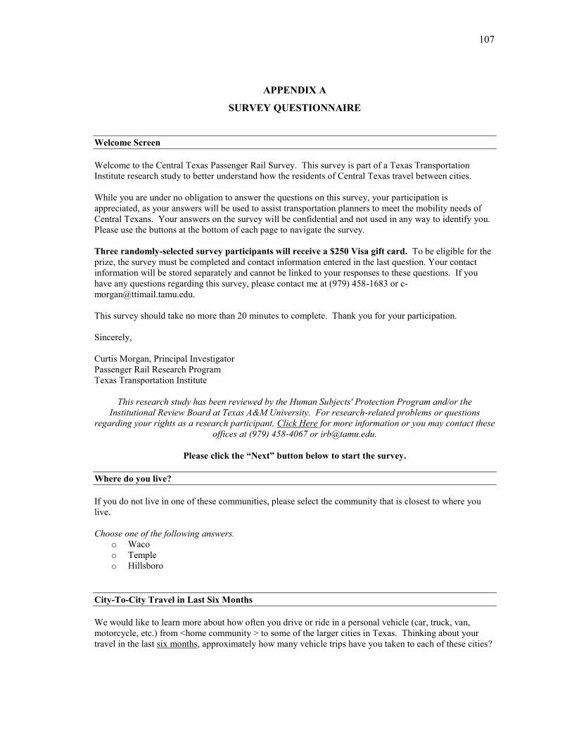
107
APPENDIX A
SURVEY QUESTIONNAIRE
Welcome Screen
Welcome to the Central Texas Passenger Rail Survey. This survey is part of a Texas Transportation
Institute research study to better understand how the residents of Central Texas travel between cities.
While you are under no obligation to answer the questions on this survey, your participation is
appreciated, as your answers will be used to assist transportation planners to meet the mobility needs of
Central Texans. Your answers on the survey will be confidential and not used in any way to identify you.
Please use the buttons at the bottom of each page to navigate the survey.
Three randomly-selected survey participants will receive a $250 Visa gift card. To be eligible for the
prize, the survey must be completed and contact information entered in the last question. Your contact
information will be stored separately and cannot be linked to your responses to these questions. If you
have any questions regarding this survey, please contact me at (979) 458-1683 or c-
This survey should take no more than 20 minutes to complete. Thank you for your participation.
Sincerely,
Curtis Morgan, Principal Investigator
Passenger Rail Research Program
Texas Transportation Institute
This research study has been reviewed by the Human Subjects' Protection Program and/or the
Institutional Review Board at Texas A&M University. For research-related problems or questions
regarding your rights as a research participant, Click Here for more information or you may contact these
offices at (979) 458-4067 or [email protected].
Please click the “Next” button below to start the survey.
Where do you live?
If you do not live in one of these communities, please select the community that is closest to where you
live.
Choose one of the following answers.
o Waco
o Temple
o Hillsboro
City-To-City Travel in Last Six Months
We would like to learn more about how often you drive or ride in a personal vehicle (car, truck, van,
motorcycle, etc.) from <home community > to some of the larger cities in Texas. Thinking about your
travel in the last six months, approximately how many vehicle trips have you taken to each of these cities?

108
Please consider only trips made in a personal vehicle, and do not include any trips you made that might
have passed through one of these cities to get to another destination. Please indicate the approximate
number of trips to each city by trip purpose (business or personal).
Business Personal (Non-Business)
Austin
o None
o 1-4 Trips
o 5-9 Trips
o 10 or More Trips
o None
o 1-4 Trips
o 5-9 Trips
o 10 or More Trips
Dallas
o None
o 1-4 Trips
o 5-9 Trips
o 10 or More Trips
o None
o 1-4 Trips
o 5-9 Trips
o 10 or More Trips
Fort Worth
o None
o 1-4 Trips
o 5-9 Trips
o 10 or More Trips
o None
o 1-4 Trips
o 5-9 Trips
o 10 or More Trips
Houston
o None
o 1-4 Trips
o 5-9 Trips
o 10 or More Trips
o None
o 1-4 Trips
o 5-9 Trips
o 10 or More Trips
San Antonio
o None
o 1-4 Trips
o 5-9 Trips
o 10 or More Trips
o None
o 1-4 Trips
o 5-9 Trips
o 10 or More Trips
When thinking about the purpose of your trip, please consider the following definitions:
Business: Any trips related to your employment or business activities such as meetings, sales,
conferences, or to purchase supplies or equipment for your business.
Personal (Non-Business): Any trips for personal reasons, such as visiting family or friends,
shopping, medical appointments, travel for educational purposes, etc.
Note: Options provided in each cell above in the form of a drop-down box.
Travel Choices Introduction
A new passenger rail system is being planned for Texas. The system would connect <home community>
to cities along the Interstate 35 corridor including Austin, Dallas, and San Antonio. Stations in those cities
would be in or near the downtown areas of those cities, and would be connected to major businesses and
tourist attractions via local transportation options or within walking distance.
Passenger trains would consist of the following amenities:
Modern and spacious passenger coach cars, containing two wide, comfortable, reclining seats on
each side of a center aisle, as shown below
Electronic outlets at each seat for laptop computers or other devices
Free high-speed wireless internet access
Passengers would be free to move around the train at all times while traveling. Each train car would
include restrooms, and each train would have a café car with food and drinks available for purchase.
Please click the “Next” button to answer questions regarding train travel.
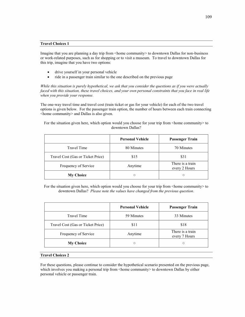
109
Travel Choices 1
Imagine that you are planning a day trip from <home community> to downtown Dallas for non-business
or work-related purposes, such as for shopping or to visit a museum. To travel to downtown Dallas for
this trip, imagine that you have two options:
drive yourself in your personal vehicle
ride in a passenger train similar to the one described on the previous page
While this situation is purely hypothetical, we ask that you consider the questions as if you were actually
faced with this situation, these travel choices, and your own personal constraints that you face in real life
when you provide your response.
The one-way travel time and travel cost (train ticket or gas for your vehicle) for each of the two travel
options is given below. For the passenger train option, the number of hours between each train connecting
<home community> and Dallas is also given.
For the situation given here, which option would you choose for your trip from <home community> to
downtown Dallas?
Personal Vehicle Passenger Train
Travel Time 80 Minutes 70 Minutes
Travel Cost (Gas or Ticket Price) $15 $31
Frequency of Service Anytime There is a train
every 2 Hours
My Choice
For the situation given here, which option would you choose for your trip from <home community> to
downtown Dallas? Please note the values have changed from the previous question.
Personal Vehicle Passenger Train
Travel Time 59 Minutes 33 Minutes
Travel Cost (Gas or Ticket Price) $11 $18
Frequency of Service Anytime There is a train
every 7 Hours
My Choice
Travel Choices 2
For these questions, please continue to consider the hypothetical scenario presented on the previous page,
which involves you making a personal trip from <home community> to downtown Dallas by either
personal vehicle or passenger train.

110
Contains similar structure and choices as “Travel Choices 1” except there is a different set of travel
times, travel costs, and rail service headway/frequency for each travel choice.
Travel Choices 3
Contains similar wording, structure, and choices as “Travel Choices 2” except there is a different set of
travel times, travel costs, and rail service headway/frequency for each travel choice.
Experience with Rail Travel
Please indicate your level of familiarity or experience with the following types of rail travel.
Note: Responses for each item given on a four-point scale as follows: Extensive Experience, Some
Experience, Heard of it But No Experience, Never Heard of It.
Light Rail Service (Dallas DART, Houston Metro)
Commuter Rail Service (Trinity Railway Express, Capital Metro)
Intercity Passenger Rail Service within Texas (Amtrak Texas Eagle, Heartland Flyer, Sunset
Limited)
Other Intercity Passenger Rail Service Outside of Texas
High-Speed Intercity Passenger Rail in the Northeast United States
High-Speed Intercity Passenger Rail in Europe or Asia
Your Opinions 1
Please indicate your level of agreement with the following statements related to your use of possible
new intercity passenger rail service for traveling out of town.
Note: Responses for each item given on a seven-point scale as follows: Strongly Disagree, Disagree,
Somewhat Disagree, Neither Disagree or Agree, Somewhat Agree, Agree, Strongly Agree.
I would travel out of town more often if I could use passenger rail for some trips.
If new intercity passenger rail service was established in my community, I would ride it once or
twice just to see what it is like.
New intercity passenger rail service in my community would not affect how I travel for trips out
of town.
Travel on intercity passenger rail would be safer than driving.
Travel on intercity passenger rail would be more efficient than driving.
Travel on intercity passenger rail would be more enjoyable than driving.
Travel on intercity passenger rail would be more reliable than driving.
Travel on intercity passenger rail would be more environmentally-friendly than driving.
Your Opinions 2
Please indicate your level of agreement with the following statements regarding the impacts of
possible new intercity passenger rail service on your community.
Note: Responses for each item given on a seven-point scale as follows: Strongly Disagree, Disagree,
Somewhat Disagree, Neither Disagree or Agree, Somewhat Agree, Agree, Strongly Agree.
New intercity passenger rail service would attract new businesses and jobs to my community.
New intercity passenger rail service would allow local businesses to be more competitive.
New intercity passenger rail service would attract out of town visitors and tourists to my
community.
New intercity passenger rail service would improve the quality of life in my community.
New intercity passenger rail service would impact my personal life in a positive manner.
111
New intercity passenger rail service would impact my business or employment in a positive
manner.
Demographics
Finally, we would like to know a little about yourself and your household. Your responses to the
questions in this section will be used to ensure that the findings of this survey are representative of the
residents of Central Texas. Your responses will remain confidential.
What is your home ZIP code? [Text Box]
What is your age?
Choose one of the following answers.
o 18 to 24 years
o 25 to 34 years
o 35 to 44 years
o 45 to 54 years
o 55 to 64 years
o 65 to 74 years
o 75 years and over
What is your gender?
Choose one of the following answers.
o Female
o Male
How many personal vehicles (car, truck, van, motorcycle, etc.) does your household own, lease, or
otherwise have available for use?
Choose one of the following answers.
o None
o One
o Two
o Three
o Four or More
Including yourself, how many adults (age 18 and over) live in your household?
Choose one of the following answers.
o One
o Two
o Three
o Four
o Five or More
How many children (under age 18) live in your household?
Choose one of the following answers.
o None
o One

112
o Two
o Three
o Four or More
What is the highest level of education you have completed?
Choose one of the following answers.
o Less than high school
o High school graduate or equivalent
o Some college or Associate's degree
o Bachelor's degree
o Graduate or professional degree
What is your annual household income?
Choose one of the following answers.
o Less than $10,000
o $10,000 to $14,999
o $15,000 to $24,999
o $25,000 to $34,999
o $35,000 to $49,999
o $50,000 to $74,999
o $75,000 to $99,999
o $100,000 to $149,999
o $150,000 to $199,999
o $200,000 or More
Please enter any additional comments you might have about new intercity passenger rail service in
your community or this study in the box below. [Text Box]
Exit Screen
Thank you for taking time to complete this survey. If you wish to participate in the random drawing,
please click on the button below to register. The information you provide for the drawing will not be
linked to your personal information provided in this survey in any way.

113
APPENDIX B
INSTITUTIONAL REVIEW BOARD APPROVAL

114

115
APPENDIX C
DETAILS OF RAIL FARE COST PER MILE ESTIMATE
Amtrak fares were computed using ticket prices accessed from the Amtrak.com website on
January 9, 2011 quoted for travel on Tuesday, March 8, 2011. Fares given were one-way with standard
class service and the lowest available fare. Mileage between cities calculated from the Amtrak timetable.
Other per-mile fare levels from selected U.S. high-speed rail feasibility studies are also given in Table C-
1. As evidenced in Table C-1, per-mile fares for intercity passenger rail routes in the U.S. vary greatly,
and it is noted that Amtrak fares are set by the company, with input from state-level partners on state-
supported routes. Proposed high-speed passenger rail service in Texas would likely command a higher
per-mile fare than existing Texas Eagle service but would probably not be as high as the nation’s only true
high-speed rail line, the Amtrak Acela. Fare costs per-mile for studies of proposed U.S. intercity
passenger rail systems range from 16.6 cents per mile to 30 cents per mile. These estimates are for
technologies that are relevant to this research, with speeds up to 125 miles per hour. Within this range are
the per-mile fares for existing U.S. passenger rail routes that operate at those speeds using conventional
equipment, the Northeast Regional and the Keystone.
Table C-1: Rail Fare Cost per Mile for Selected U.S. Intercity Passenger Rail Routes Segment/Route Cents/Mile Source
Fort Worth-Temple/Texas Eagle 10.2 Amtrak.com 3/8/2011
Fort Worth-Oklahoma City/Heartland Flyer 12.6 Amtrak.com 3/8/2011
Fort Worth-Gainesville/Heartland Flyer 15.4 Amtrak.com 3/8/2011
Fort Worth-San Antonio/ Texas Eagle 8.8 Amtrak.com 3/8/2011
Chicago-St. Louis/Lincoln Service 8.5 Amtrak.com 3/8/2011
NY Penn-Washington D.C./Acela 59.7 Amtrak.com 3/8/2011
NY Penn-Washington D.C./NE Regional 21.7 Amtrak.com 3/8/2011
Philadelphia-Harrisburg/Keystone 23.1 Amtrak.com 3/8/2011
Seattle-Portland/Cascades 12.3 Amtrak.com 3/8/2011
Proposed Boston-Montreal HSR 26.0 Parsons Brinckerhoff
Quade & Douglas (2003)
Proposed Rocky MTN Rail 28.0 Transportation Economics and
Management Systems, Inc. (2010)
Proposed MWRRS 23.0 Transportation Economics and
Management Systems, Inc. (2004)
Proposed California HSR 9.0 Cambridge Systematics,
Inc. et al. (2006)
Proposed Florida HSR 30.0 HNTB Corporation (2003)
Proposed Alberta HSR 25.0 Transportation Economics and
Management Systems, Inc. (2008)
California North/South 16.6 Federal Railroad Administration (1997)
California South 28.5 Federal Railroad Administration (1997)
Chicago Hub 18.1 Federal Railroad Administration (1997)
Chicago-Detroit 17.0 Federal Railroad Administration (1997)
Chicago-St Louis 18.8 Federal Railroad Administration (1997)
Florida 22.3 Federal Railroad Administration (1997)
Pacific Northwest 24.7 Federal Railroad Administration (1997)
Texas Triangle 17.7 Federal Railroad Administration (1997)
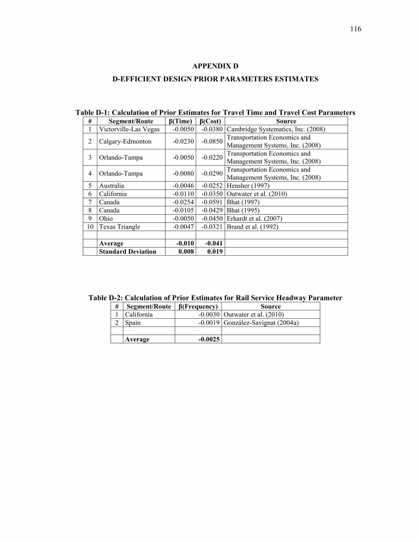
116
APPENDIX D
D-EFFICIENT DESIGN PRIOR PARAMETERS ESTIMATES
Table D-1: Calculation of Prior Estimates for Travel Time and Travel Cost Parameters # Segment/Route β(Time) β(Cost) Source
1 Victorville-Las Vegas -0.0050 -0.0380 Cambridge Systematics, Inc. (2008)
2 Calgary-Edmonton -0.0230 -0.0850 Transportation Economics and
Management Systems, Inc. (2008)
3 Orlando-Tampa -0.0050 -0.0220 Transportation Economics and
Management Systems, Inc. (2008)
4 Orlando-Tampa -0.0080 -0.0290 Transportation Economics and
Management Systems, Inc. (2008)
5 Australia -0.0046 -0.0252 Hensher (1997)
6 California -0.0110 -0.0350 Outwater et al. (2010)
7 Canada -0.0254 -0.0591 Bhat (1997)
8 Canada -0.0105 -0.0429 Bhat (1995)
9 Ohio -0.0050 -0.0450 Erhardt et al. (2007)
10 Texas Triangle -0.0047 -0.0321 Brand et al. (1992)
Average -0.010 -0.041
Standard Deviation 0.008 0.019
Table D-2: Calculation of Prior Estimates for Rail Service Headway Parameter # Segment/Route β(Frequency) Source
1 California -0.0030 Outwater et al. (2010)
2 Spain -0.0019 González-Savignat (2004a)
Average -0.0025

117
APPENDIX E
NGENE SYNTAX AND OUTPUT
NGENE Syntax
Design – Waco
;alts = auto,rail
;rows = 18
;block = 6
;eff = (mnl,d)
;rdraws = random(1000)
;model:
U(auto) = b1[n,-0.01,0.008] * x1[80,90,100] + b2[n,-0.041,0.019] *
x2[14,19,24] /
U(rail) = c1[n,0,0.5] + b1 * x3[50,55,60] + b2 *
x4[19,25,31] + b3[-0.0025] * x5[120,360,600] $
Design – Temple
;alts = auto,rail
;rows = 18
;block = 6
;eff = (mnl,d)
;rdraws = random(1000)
;model:
U(auto) = b1[n,-0.01,0.008] * x1[105,120,135] + b2[n,-
0.041,0.019] * x2[19,25,31] /
U(rail) = c1[n,0,0.5] + b1 * x3[60,70,80] + b2
* x4[25,33,41] + b3[-0.0025] * x5[120,360,600] $
Design – Hillsboro
;alts = auto,rail
;rows = 18
;block = 6
;eff = (mnl,d)
;rdraws = random(1000)
;model:
U(auto) = b1[n,-0.01,0.008] * x1[50,60,70] + b2[n,-
0.041,0.019] * x2[9,12,15] /
U(rail) = c1[n,0,0.5] + b1 * x3[30,35,40] + b2
* x4[12,16,20] + b3[-0.0025] * x5[120,360,600] $

118
NGENE Output: Waco
D error 0.000383
A error 0.00191
B estimate 81.393425
S estimate 82.461563
Prior b1 b2 b3
Fixed prior value -0.01 -0.041 -0.0025
Sp estimates 82.461563 8.170714 4.710694
Sp t-ratios 0.215839 0.685687 0.903054
Design
Choice situation auto.x1 auto.x2 rail.x3 rail.x4 rail.x5 Block
1 80 24 60 19 360 6
2 100 14 50 25 360 6
3 100 19 55 31 600 4
4 90 19 60 25 600 4
5 80 19 55 25 600 5
6 100 14 55 31 360 5
7 90 14 55 31 360 2
8 80 24 55 19 120 4
9 100 19 50 25 120 2
10 90 14 50 31 120 3
11 80 19 60 25 120 1
12 100 24 50 19 360 6
13 80 19 60 31 600 3
14 100 24 50 19 600 1
15 80 14 60 31 120 5
16 90 24 50 19 600 2
17 90 24 55 19 120 3
18 90 14 60 25 360 1

119
NGENE Output: Temple
D error 0.000221
A error 0.001001
B estimate 82.11921
S estimate 26.414453
Prior b1 b2 b3
Fixed prior value -0.01 -0.041 -0.0025
Sp estimates 26.414453 5.276794 4.466002
Sp t-ratios 0.38136 0.85324 0.927463
Design
Choice situation auto.x1 auto.x2 rail.x3 rail.x4 rail.x5 Block
1 135 31 60 25 360 4
2 135 19 70 33 600 3
3 120 25 60 41 600 5
4 135 31 60 25 600 1
5 135 19 60 41 120 2
6 105 31 80 25 360 4
7 105 31 80 25 120 2
8 105 25 80 33 360 3
9 105 19 80 41 360 1
10 120 25 70 33 600 6
11 135 25 60 33 120 6
12 105 31 80 25 600 5
13 120 19 70 41 360 1
14 120 31 70 25 120 2
15 120 25 60 33 600 3
16 120 25 70 41 360 4
17 135 19 70 41 120 5
18 105 19 80 33 120 6

120
NGENE Output: Hillsboro
D error 0.000503
A error 0.003731
B estimate 81.223362
S estimate 71.944034
Prior b1 b2 b3
Fixed prior value -0.01 -0.041 -0.0025
Sp estimates 71.944034 21.280688 4.514485
Sp t-ratios 0.231078 0.424877 0.922469
Design
Choice situation auto.x1 auto.x2 rail.x3 rail.x4 rail.x5 Block
1 50 9 40 20 120 5
2 60 12 35 20 360 6
3 50 15 40 12 120 6
4 50 12 40 20 360 1
5 50 9 40 20 360 3
6 60 15 35 12 600 4
7 60 9 35 16 360 2
8 50 15 35 12 120 2
9 70 15 30 12 360 1
10 60 9 35 16 600 5
11 70 9 30 16 120 1
12 70 12 30 20 600 3
13 60 15 40 16 600 2
14 50 12 35 12 360 4
15 70 15 30 12 120 5
16 70 12 30 16 600 6
17 70 9 30 20 120 4
18 60 12 40 16 600 3
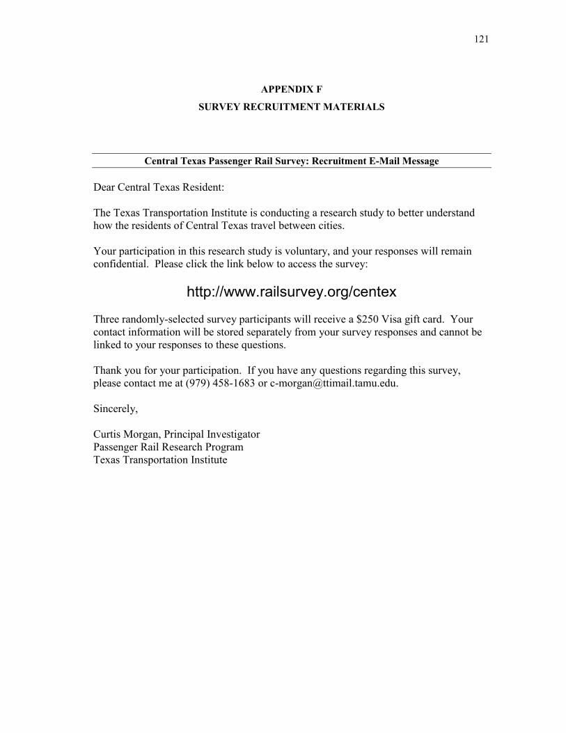
121
APPENDIX F
SURVEY RECRUITMENT MATERIALS
Central Texas Passenger Rail Survey: Recruitment E-Mail Message
Dear Central Texas Resident:
The Texas Transportation Institute is conducting a research study to better understand
how the residents of Central Texas travel between cities.
Your participation in this research study is voluntary, and your responses will remain
confidential. Please click the link below to access the survey:
http://www.railsurvey.org/centex
Three randomly-selected survey participants will receive a $250 Visa gift card. Your
contact information will be stored separately from your survey responses and cannot be
linked to your responses to these questions.
Thank you for your participation. If you have any questions regarding this survey,
please contact me at (979) 458-1683 or [email protected].
Sincerely,
Curtis Morgan, Principal Investigator
Passenger Rail Research Program
Texas Transportation Institute

122
Central Texas Passenger Rail Survey: Recruitment Newspaper Advertisement
Central Texas Passenger Rail Survey: Recruitment Postcard

123
APPENDIX G
SURVEY SAMPLE WEIGHTS CALCULATIONS
Additional details for calculation of the sample weights used to adjust the survey responses to
reflect the community-level distributions of age group and household income by community are provided
below. The following tables show the raw count of the total number of survey respondents in each age
group/household income combination as well as the first and second iterations of the raking algorithm.
The survey sample weights shown in Table 6 and Table 7 were obtained by dividing the individual cell
values from the final iteration by the corresponding cell values in the raw counts table.
Table G-1: Survey Sample Weights: Waco (Raw Counts)
Age Group/
Household
Income Les
s th
an
$2
5,0
00
$2
5,0
00
-
$4
9,9
99
$5
0,0
00
-
$7
4,9
99
$7
5,0
00
-
$9
9,9
99
$1
00
,00
0-
$1
49
,99
9
$1
50
,00
0-
$1
99
,99
9
$2
00
,00
0
or
Mo
re
18 to 24 years 7 8 1 0 1 0 0
25 to 34 years 9 28 33 10 12 5 1
35 to 44 years 2 15 29 18 16 2 4
45 to 54 years 7 31 34 30 26 13 8
55 to 64 years 6 30 49 23 36 10 5
65 years and over 9 18 14 8 3 2 2
Table G-2: Survey Sample Weights: Waco (Raking Algorithm First Iteration)
Age Group/
Household
Income Les
s th
an
$2
5,0
00
$2
5,0
00
-
$4
9,9
99
$5
0,0
00
-
$7
4,9
99
$7
5,0
00
-
$9
9,9
99
$1
00
,00
0-
$1
49
,99
9
$1
50
,00
0-
$1
99
,99
9
$2
00
,00
0
or
Mo
re
Fac
tor
18 to 24 years 61 70 9 0 9 0 0 8.745
25 to 34 years 10 31 36 11 13 5 1 1.092
35 to 44 years 2 14 26 16 14 2 4 0.904
45 to 54 years 4 17 19 16 14 7 4 0.548
55 to 64 years 2 12 20 9 15 4 2 0.411
65 years and over 14 27 21 12 5 3 3 1.511
Table G-3: Survey Sample Weights: Waco (Raking Algorithm Second Iteration)
Age Group/
Household
Income Les
s th
an
$2
5,0
00
$2
5,0
00
-
$4
9,9
99
$5
0,0
00
-
$7
4,9
99
$7
5,0
00
-
$9
9,9
99
$1
00
,00
0-
$1
49
,99
9
$1
50
,00
0-
$1
99
,99
9
$2
00
,00
0
or
Mo
re
18 to 24 years 149 63 6 0 5 0 0
25 to 34 years 24 28 24 7 7 2 1
35 to 44 years 4 12 17 11 8 1 2
45 to 54 years 9 15 12 11 8 2 3
55 to 64 years 6 11 13 6 8 1 1
65 years and over 33 25 14 8 2 1 2
Factor 2.430 0.907 0.666 0.677 0.529 0.343 0.646

124
Table G-4: Survey Sample Weights: Temple (Raw Counts)
Age Group/
Household
Income Les
s th
an
$2
5,0
00
$2
5,0
00
-
$4
9,9
99
$5
0,0
00
-
$7
4,9
99
$7
5,0
00
-
$9
9,9
99
$1
00
,00
0-
$1
49
,99
9
$1
50
,00
0-
$1
99
,99
9
$2
00
,00
0
or
Mo
re
18 to 24 years 2 6 0 1 1 1 0
25 to 34 years 5 22 19 16 6 3 0
35 to 44 years 5 19 19 20 13 6 4
45 to 54 years 9 22 31 24 23 10 4
55 to 64 years 8 22 29 10 24 5 11
65 years and over 6 11 21 10 8 4 2
Table G-5: Survey Sample Weights: Temple (Raking Algorithm First Iteration)
Age Group/
Household
Income Les
s th
an
$2
5,0
00
$2
5,0
00
-
$4
9,9
99
$5
0,0
00
-
$7
4,9
99
$7
5,0
00
-
$9
9,9
99
$1
00
,00
0-
$1
49
,99
9
$1
50
,00
0-
$1
99
,99
9
$2
00
,00
0
or
Mo
re
Fac
tor
18 to 24 years 11 32 0 5 5 5 0 5.254
25 to 34 years 7 29 25 21 8 4 0 1.313
35 to 44 years 4 16 16 17 11 5 3 0.856
45 to 54 years 6 15 21 16 15 7 3 0.672
55 to 64 years 5 14 18 6 15 3 7 0.623
65 years and over 8 15 29 14 11 6 3 1.398
Table G-6: Survey Sample Weights: Temple (Raking Algorithm Second Iteration)
Age Group/
Household
Income Les
s th
an
$2
5,0
00
$2
5,0
00
-
$4
9,9
99
$5
0,0
00
-
$7
4,9
99
$7
5,0
00
-
$9
9,9
99
$1
00
,00
0-
$1
49
,99
9
$1
50
,00
0-
$1
99
,99
9
$2
00
,00
0
or
Mo
re
18 to 24 years 34 29 0 3 4 3 0
25 to 34 years 21 26 19 14 6 2 0
35 to 44 years 14 15 12 11 9 3 3
45 to 54 years 20 14 16 11 12 4 2
55 to 64 years 16 13 14 4 12 2 5
65 years and over 27 14 22 9 9 4 2
Factor 3.247 0.913 0.755 0.663 0.808 0.626 0.760

125
APPENDIX H
NLOGIT SYNTAX
Variable Key:
Variable Name Symbol Auto Model Symbol Rail Model
Travel Time Btt TT TT
Travel Cost Btc TC TC
Rail Service Frequency Bfreq FREQ
Rail ASC ASC ASC
HHINC B1 HHINC88 B2 HHINC38
AGE B4 AGE21 B5 AGE65
VEHICLE B9 VEH4PLUS B8 VEHONE
EDUCATE B10 EDU2 B13 EDU3
ADULT B14 ADULT1
CHILD B15 CHILD1 B16 CHILDN
Rail Travel Factor Btravel TRAVELF
Rail Impact Factor Bimpact IMPACTF
Rail Experience Factor Bexper RAILF
Pooled Model NLOGIT Syntax:
?----SET SAMPLE----
SAMPLE
;All$
CALC;LIST
;ran(91783)$
INCLUDE
;New
;DESIGN=1$
?----Random Parameters Model for Pooled Model (Table 17)
RPLOGIT
;Lhs=CHOICE
;Choices=car,train
;Halton;Pts=500;maxit=25
;Fcn=btime[t]
;Wts=WTSWUTC
;Model:
U(car)=btime*TT+bcost*TC+b4*age21+b15*child1/
U(train)=btime*TT+bcost*TC+bfreq*FREQ+b2*hhinc38+b8*vehone+b13*edu3+btr
avel*travelf+bimpact*impactf+bexper*railf+ASC
;Crosstab$
Waco Model NLOGIT Syntax:
?----SET SAMPLE----
INCLUDE
;New
;DESIGN=1 & CITY=1$
?----Random Parameters Model for Waco Model (Table 19)
RPLOGIT
;Lhs=CHOICE

126
;Choices=car,train
;Halton;Pts=500;maxit=25
;Fcn=btime[t]
;Wts=WTSWUTC
;Model:
U(car)=btime*TT+bcost*TC+b4*age21+b15*child1/
U(train)=btime*TT+bcost*TC+bfreq*FREQ+b2*hhinc38+b8*vehone+b16*childn+b
travel*travelf+bimpact*impact
;Crosstab$
Temple Model NLOGIT Syntax:
?----Random Parameters Model for Temple Model (Table 19)
INCLUDE
;New
;DESIGN=1 & CITY=2$
RPLOGIT
;Lhs=CHOICE
;Choices=car,train
;Halton;Pts=500;maxit=25
;Fcn=btime[t]
;Wts=WTSWUTC
;Model:
U(car)=btime*TT+bcost*TC+b9*veh4plus+b15*child1/
U(train)=btime*TT+bcost*TC+bfreq*FREQ+b13*edu3+btravel*travelf+bimpact*
impactf+bexper*railf+ASC
;Crosstab$
Text-Only Model NLOGIT Syntax:
?----Random Parameters Model for Text-Only Model (Table 20/21)
INCLUDE
;New
;DESIGN=1 & PHOTO1=1$
RPLOGIT
;Lhs=CHOICE
;Choices=car,train
;Halton;Pts=500;maxit=25
;Fcn=btime[t]
;Wts=WTSWUTC
;Model:
U(car)=btime*TT+bcost*TC/
U(train)=btime*TT+bcost*TC+bfreq*FREQ+b2*hhinc38+b5*age65+b14*adult1+bt
ravel*travelf+bimpact*impactf+bexper*railf
;Crosstab$
Photos Model NLOGIT Syntax:
?----Random Parameters Model for Photos Model (Table 20)
INCLUDE
;New
;DESIGN=1 & PHOTO2=2$
RPLOGIT
;Lhs=CHOICE
;Choices=car,train

127
;Halton;Pts=500;maxit=25
;Fcn=btime[t]
;Wts=WTSWUTC
;Model:
U(car)=btime*TT+bcost*TC+b4*age21+b15*child1/
U(train)=btime*TT+bcost*TC+bfreq*FREQ+b2*hhinc38+b8*vehone+bimpact*impa
ctf+ASC
;Crosstab$
Typical Model NLOGIT Syntax:
?----Random Parameters Model for Typical Model (Table 21)
INCLUDE
;New
;DESIGN=1 & PHOTO1=2$
RPLOGIT
;Lhs=CHOICE
;Choices=car,train
;Halton;Pts=500;maxit=25
;Fcn=btime[t]
;Wts=WTSWUTC
;Model:
U(car)=btime*TT+bcost*TC+b4*age21+b15*child1/
U(train)=btime*TT+bcost*TC+bfreq*FREQ+b2*hhinc38+b8*vehone+bimpact*impa
ctf+ASC
;Crosstab$
Flashy Model NLOGIT Syntax:
?----Random Parameters Model for Flashy Model (Table 21)
INCLUDE
;New
;DESIGN=1 & PHOTO1=3$
RPLOGIT
;Lhs=CHOICE
;Choices=car,train
;Halton;Pts=500;maxit=25
;Fcn=btime[t]
;Wts=WTSWUTC
;Model:
U(car)=btime*TT+bcost*TC/
U(train)=btime*TT+bcost*TC+bfreq*FREQ+b13*edu3+b14*adult1+bimpact*impac
tf+ASC
;Crosstab$
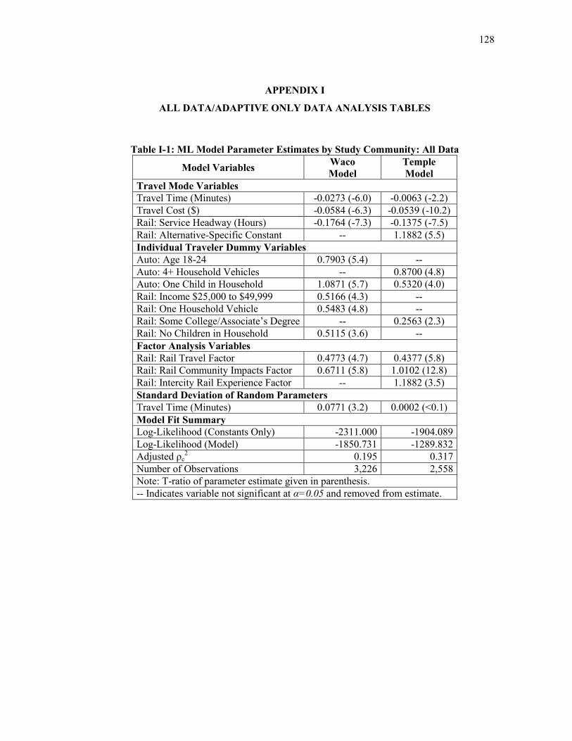
128
APPENDIX I
ALL DATA/ADAPTIVE ONLY DATA ANALYSIS TABLES
Table I-1: ML Model Parameter Estimates by Study Community: All Data
Model Variables Waco
Model
Temple
Model
Travel Mode Variables
Travel Time (Minutes) -0.0273 (-6.0) -0.0063 (-2.2)
Travel Cost ($) -0.0584 (-6.3) -0.0539 (-10.2)
Rail: Service Headway (Hours) -0.1764 (-7.3) -0.1375 (-7.5)
Rail: Alternative-Specific Constant -- 1.1882 (5.5)
Individual Traveler Dummy Variables
Auto: Age 18-24 0.7903 (5.4) --
Auto: 4+ Household Vehicles -- 0.8700 (4.8)
Auto: One Child in Household 1.0871 (5.7) 0.5320 (4.0)
Rail: Income $25,000 to $49,999 0.5166 (4.3) --
Rail: One Household Vehicle 0.5483 (4.8) --
Rail: Some College/Associate’s Degree -- 0.2563 (2.3)
Rail: No Children in Household 0.5115 (3.6) --
Factor Analysis Variables
Rail: Rail Travel Factor 0.4773 (4.7) 0.4377 (5.8)
Rail: Rail Community Impacts Factor 0.6711 (5.8) 1.0102 (12.8)
Rail: Intercity Rail Experience Factor -- 1.1882 (3.5)
Standard Deviation of Random Parameters
Travel Time (Minutes) 0.0771 (3.2) 0.0002 (<0.1)
Model Fit Summary
Log-Likelihood (Constants Only) -2311.000 -1904.089
Log-Likelihood (Model) -1850.731 -1289.832
Adjusted ρc2 0.195 0.317
Number of Observations 3,226 2,558
Note: T-ratio of parameter estimate given in parenthesis.
-- Indicates variable not significant at α=0.05 and removed from estimate.
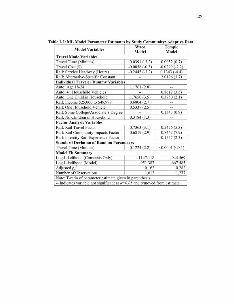
129
Table I-2: ML Model Parameter Estimates by Study Community: Adaptive Data
Model Variables Waco
Model
Temple
Model
Travel Mode Variables
Travel Time (Minutes) -0.0391 (-3.2) 0.0052 (0.7)
Travel Cost ($) -0.0058 (-0.3) -0.0299 (-2.2)
Rail: Service Headway (Hours) -0.2445 (-3.2) 0.1343 (-4.4)
Rail: Alternative-Specific Constant -- 2.0196 (3.7)
Individual Traveler Dummy Variables
Auto: Age 18-24 1.1761 (2.8) --
Auto: 4+ Household Vehicles -- 0.8612 (3.5)
Auto: One Child in Household 1.7650 (3.5) 0.3750 (2.1)
Rail: Income $25,000 to $49,999 0.6804 (2.7) --
Rail: One Household Vehicle 0.5337 (2.5) --
Rail: Some College/Associate’s Degree -- 0.1343 (0.9)
Rail: No Children in Household 0.3184 (1.3) --
Factor Analysis Variables
Rail: Rail Travel Factor 0.7363 (3.1) 0.5476 (5.3)
Rail: Rail Community Impacts Factor 0.6819 (2.9) 0.8467 (7.9)
Rail: Intercity Rail Experience Factor -- 0.1557 (2.3)
Standard Deviation of Random Parameters
Travel Time (Minutes) 0.1224 (2.2) <0.0001 (<0.1)
Model Fit Summary
Log-Likelihood (Constants Only) -1147.118 -944.569
Log-Likelihood (Model) -951.387 -667.485
Adjusted ρc2 0.162 0.282
Number of Observations 1,613 1,277
Note: T-ratio of parameter estimate given in parenthesis.
-- Indicates variable not significant at α=0.05 and removed from estimate.

130
Table I-3: ML Model Parameter Estimates by Text-Only and Image: All Data
Model Variables Text-Only
Model
Photos
Model
Travel Mode Variables
Travel Time (Minutes) -0.0187 (-5.3) 0.0005 (0.2)
Travel Cost ($) -0.0681 (-7.5) -0.0501 (-8.9)
Rail: Service Headway (Hours) -0.1046 (-4.5) -0.2144 (-11.0)
Rail: Alternative-Specific Constant -- 1.8065 (9.1)
Individual Traveler Dummy Variables
Auto: Age 18-24 -- 0.6916 (6.8)
Auto: One Child in Household -- 1.3015 (9.1)
Rail: Income $25,000 to $49,999 0.4738 (3.4) 0.4464 (4.8)
Rail: Age 65 or Older 1.0750 (4.2) --
Rail: One Household Vehicle -- 0.1947 (2.3)
Rail: One Adult in Household 0.4809 (3.1) --
Factor Analysis Variables
Rail: Rail Travel Factor 0.7810 (6.2) --
Rail: Rail Community Impacts Factor 0.5466 (4.9) 1.0804 (13.5)
Rail: Intercity Rail Experience Factor 0.5110 (6.6) --
Standard Deviation of Random Parameters
Travel Time (Minutes) 0.0387 (1.8) 0.0222 (1.0)
Model Fit Summary
Log-Likelihood (Constants Only) -1385.183 -2831.661
Log-Likelihood (Model) -975.314 -2199.939
Adjusted ρc2 0.289 0.220
Number of Observations 1,884 3,978
Note: T-ratio of parameter estimate given in parenthesis.
-- Indicates variable not significant at α=0.05 and removed from estimate.
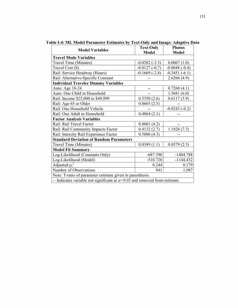
131
Table I-4: ML Model Parameter Estimates by Text-Only and Image: Adaptive Data
Model Variables Text-Only
Model
Photos
Model
Travel Mode Variables
Travel Time (Minutes) -0.0202 (-3.3) 0.0067 (1.0)
Travel Cost ($) -0.0127 (-0.7) -0.0048 (-0.4)
Rail: Service Headway (Hours) -0.1669 (-2.8) -0.3451 (-6.1)
Rail: Alternative-Specific Constant -- 2.6266 (4.9)
Individual Traveler Dummy Variables
Auto: Age 18-24 -- 0.7260 (4.1)
Auto: One Child in Household -- 1.5681 (6.0)
Rail: Income $25,000 to $49,999 0.5350 (2.6) 0.6117 (3.9)
Rail: Age 65 or Older 0.8665 (2.5) --
Rail: One Household Vehicle -- -0.0243 (-0.2)
Rail: One Adult in Household 0.4864 (2.1) --
Factor Analysis Variables
Rail: Rail Travel Factor 0.8001 (4.2) --
Rail: Rail Community Impacts Factor 0.4132 (2.7) 1.1826 (7.3)
Rail: Intercity Rail Experience Factor 0.5806 (4.3) --
Standard Deviation of Random Parameters
Travel Time (Minutes) 0.0389 (1.1) 0.0579 (2.5)
Model Fit Summary
Log-Likelihood (Constants Only) -687.390 -1404.788
Log-Likelihood (Model) -510.720 -1144.432
Adjusted ρc2 0.244 0.179
Number of Observations 941 1,987
Note: T-ratio of parameter estimate given in parenthesis.
-- Indicates variable not significant at α=0.05 and removed from estimate.
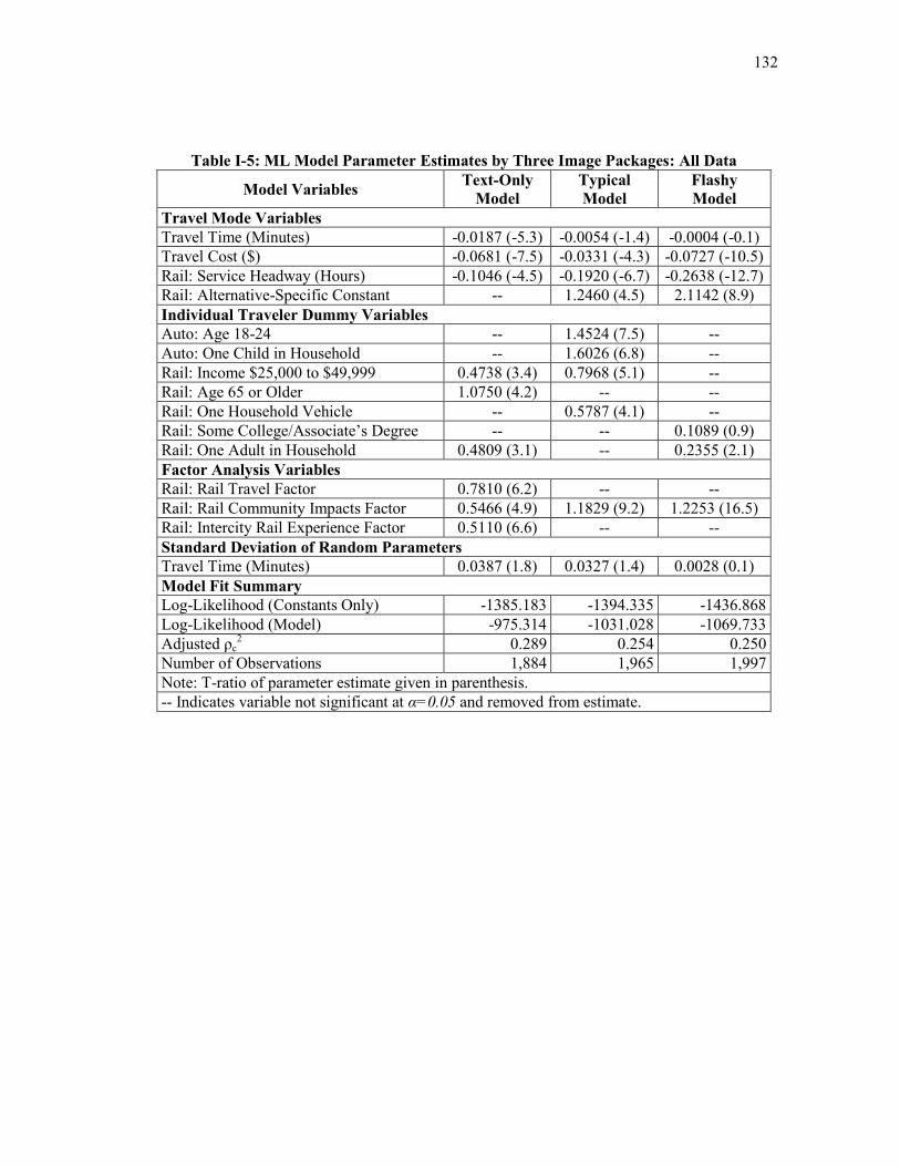
132
Table I-5: ML Model Parameter Estimates by Three Image Packages: All Data
Model Variables Text-Only
Model
Typical
Model
Flashy
Model
Travel Mode Variables
Travel Time (Minutes) -0.0187 (-5.3) -0.0054 (-1.4) -0.0004 (-0.1)
Travel Cost ($) -0.0681 (-7.5) -0.0331 (-4.3) -0.0727 (-10.5)
Rail: Service Headway (Hours) -0.1046 (-4.5) -0.1920 (-6.7) -0.2638 (-12.7)
Rail: Alternative-Specific Constant -- 1.2460 (4.5) 2.1142 (8.9)
Individual Traveler Dummy Variables
Auto: Age 18-24 -- 1.4524 (7.5) --
Auto: One Child in Household -- 1.6026 (6.8) --
Rail: Income $25,000 to $49,999 0.4738 (3.4) 0.7968 (5.1) --
Rail: Age 65 or Older 1.0750 (4.2) -- --
Rail: One Household Vehicle -- 0.5787 (4.1) --
Rail: Some College/Associate’s Degree -- -- 0.1089 (0.9)
Rail: One Adult in Household 0.4809 (3.1) -- 0.2355 (2.1)
Factor Analysis Variables
Rail: Rail Travel Factor 0.7810 (6.2) -- --
Rail: Rail Community Impacts Factor 0.5466 (4.9) 1.1829 (9.2) 1.2253 (16.5)
Rail: Intercity Rail Experience Factor 0.5110 (6.6) -- --
Standard Deviation of Random Parameters
Travel Time (Minutes) 0.0387 (1.8) 0.0327 (1.4) 0.0028 (0.1)
Model Fit Summary
Log-Likelihood (Constants Only) -1385.183 -1394.335 -1436.868
Log-Likelihood (Model) -975.314 -1031.028 -1069.733
Adjusted ρc2 0.289 0.254 0.250
Number of Observations 1,884 1,965 1,997
Note: T-ratio of parameter estimate given in parenthesis.
-- Indicates variable not significant at α=0.05 and removed from estimate.

133
Table I-6: ML Model Parameter Estimates by Three Image Packages: Adaptive Data
Model Variables Text-Only
Model
Typical
Model
Flashy
Model
Travel Mode Variables
Travel Time (Minutes) -0.0202 (-3.3) -0.0064 (-0.8) 0.0120 (1.3)
Travel Cost ($) -0.0127 (-0.7) -0.0297 (-1.7) -0.0020 (-0.1)
Rail: Service Headway (Hours) -0.1669 (-2.8) -0.0933 (-1.7) -0.5047 (-6.0)
Rail: Alternative-Specific Constant -- 0.7249 (1.3) 3.6717 (4.8)
Individual Traveler Dummy Variables
Auto: Age 18-24 -- 1.3927 (5.2) --
Auto: One Child in Household -- 1.3875 (4.6) --
Rail: Income $25,000 to $49,999 0.5350 (2.6) 0.6727 (3.3) --
Rail: Age 65 or Older 0.8665 (2.5) -- --
Rail: One Household Vehicle -- 0.3236 (1.8) --
Rail: Some College/Associate’s Degree -- -- -0.0542 (-0.3)
Rail: One Adult in Household 0.4864 (2.1) -- 0.0932 (0.5)
Factor Analysis Variables
Rail: Rail Travel Factor 0.8001 (4.2) -- --
Rail: Rail Community Impacts Factor 0.4132 (2.7) 1.0382 (6.3) 1.3125 (6.4)
Rail: Intercity Rail Experience Factor 0.5806 (4.3) -- --
Standard Deviation of Random Parameters
Travel Time (Minutes) 0.0389 (1.1) 0.0205 (0.4) 0.0502 (1.8)
Model Fit Summary
Log-Likelihood (Constants Only) -687.390 -695.322 -708.793
Log-Likelihood (Model) -510.720 -551.734 -546.694
Adjusted ρc2 0.244 0.193 0.219
Number of Observations 941 982 997
Note: T-ratio of parameter estimate given in parenthesis.
-- Indicates variable not significant at α=0.05 and removed from estimate.
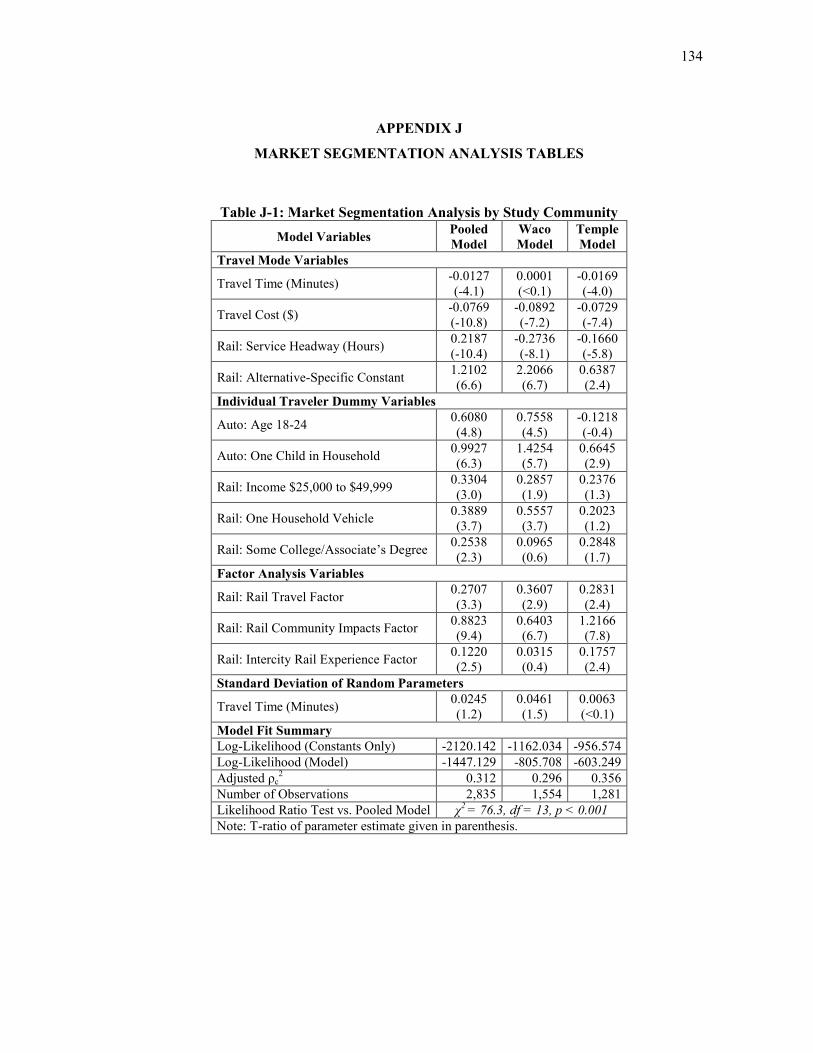
134
APPENDIX J
MARKET SEGMENTATION ANALYSIS TABLES
Table J-1: Market Segmentation Analysis by Study Community
Model Variables Pooled
Model
Waco
Model
Temple
Model
Travel Mode Variables
Travel Time (Minutes) -0.0127
(-4.1)
0.0001
(<0.1)
-0.0169
(-4.0)
Travel Cost ($) -0.0769
(-10.8)
-0.0892
(-7.2)
-0.0729
(-7.4)
Rail: Service Headway (Hours) 0.2187
(-10.4)
-0.2736
(-8.1)
-0.1660
(-5.8)
Rail: Alternative-Specific Constant 1.2102
(6.6)
2.2066
(6.7)
0.6387
(2.4)
Individual Traveler Dummy Variables
Auto: Age 18-24 0.6080
(4.8)
0.7558
(4.5)
-0.1218
(-0.4)
Auto: One Child in Household 0.9927
(6.3)
1.4254
(5.7)
0.6645
(2.9)
Rail: Income $25,000 to $49,999 0.3304
(3.0)
0.2857
(1.9)
0.2376
(1.3)
Rail: One Household Vehicle 0.3889
(3.7)
0.5557
(3.7)
0.2023
(1.2)
Rail: Some College/Associate’s Degree 0.2538
(2.3)
0.0965
(0.6)
0.2848
(1.7)
Factor Analysis Variables
Rail: Rail Travel Factor 0.2707
(3.3)
0.3607
(2.9)
0.2831
(2.4)
Rail: Rail Community Impacts Factor 0.8823
(9.4)
0.6403
(6.7)
1.2166
(7.8)
Rail: Intercity Rail Experience Factor 0.1220
(2.5)
0.0315
(0.4)
0.1757
(2.4)
Standard Deviation of Random Parameters
Travel Time (Minutes) 0.0245
(1.2)
0.0461
(1.5)
0.0063
(<0.1)
Model Fit Summary
Log-Likelihood (Constants Only) -2120.142 -1162.034 -956.574
Log-Likelihood (Model) -1447.129 -805.708 -603.249
Adjusted ρc2 0.312 0.296 0.356
Number of Observations 2,835 1,554 1,281
Likelihood Ratio Test vs. Pooled Model χ2 = 76.3, df = 13, p < 0.001
Note: T-ratio of parameter estimate given in parenthesis.
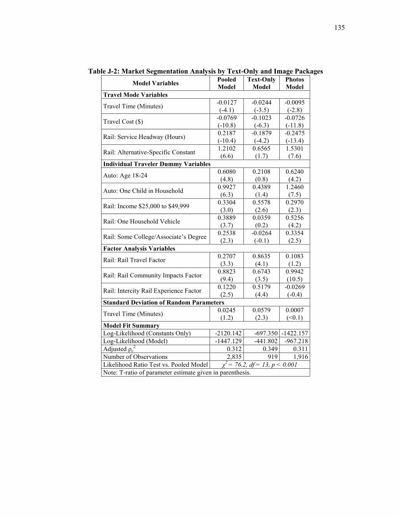
135
Table J-2: Market Segmentation Analysis by Text-Only and Image Packages
Model Variables Pooled
Model
Text-Only
Model
Photos
Model
Travel Mode Variables
Travel Time (Minutes) -0.0127
(-4.1)
-0.0244
(-3.5)
-0.0095
(-2.8)
Travel Cost ($) -0.0769
(-10.8)
-0.1023
(-6.3)
-0.0726
(-11.8)
Rail: Service Headway (Hours) 0.2187
(-10.4)
-0.1879
(-4.2)
-0.2475
(-13.4)
Rail: Alternative-Specific Constant 1.2102
(6.6)
0.6565
(1.7)
1.5301
(7.6)
Individual Traveler Dummy Variables
Auto: Age 18-24 0.6080
(4.8)
0.2108
(0.8)
0.6240
(4.2)
Auto: One Child in Household 0.9927
(6.3)
0.4389
(1.4)
1.2460
(7.5)
Rail: Income $25,000 to $49,999 0.3304
(3.0)
0.5578
(2.6)
0.2970
(2.3)
Rail: One Household Vehicle 0.3889
(3.7)
0.0359
(0.2)
0.5256
(4.2)
Rail: Some College/Associate’s Degree 0.2538
(2.3)
-0.0264
(-0.1)
0.3354
(2.5)
Factor Analysis Variables
Rail: Rail Travel Factor 0.2707
(3.3)
0.8635
(4.1)
0.1083
(1.2)
Rail: Rail Community Impacts Factor 0.8823
(9.4)
0.6743
(3.5)
0.9942
(10.5)
Rail: Intercity Rail Experience Factor 0.1220
(2.5)
0.5179
(4.4)
-0.0269
(-0.4)
Standard Deviation of Random Parameters
Travel Time (Minutes) 0.0245
(1.2)
0.0579
(2.3)
0.0007
(<0.1)
Model Fit Summary
Log-Likelihood (Constants Only) -2120.142 -697.350 -1422.157
Log-Likelihood (Model) -1447.129 -441.802 -967.218
Adjusted ρc2 0.312 0.349 0.311
Number of Observations 2,835 919 1,916
Likelihood Ratio Test vs. Pooled Model χ2 = 76.2, df = 13, p < 0.001
Note: T-ratio of parameter estimate given in parenthesis.

136
Table J-3: Market Segmentation Analysis by Three Image Packages
Model Variables Pooled
Model
Text-Only
Model
Typical
Model
Flashy
Model
Travel Mode Variables
Travel Time (Minutes) -0.0127
(-4.1)
-0.0244
(-3.5)
-0.0131
(-2.3)
-0.0123
(-2.4)
Travel Cost ($) -0.0769
(-10.8)
-0.1023
(-6.3)
-0.0481
(-4.5)
-0.1057
(-11.1)
Rail: Service Headway (Hours) 0.2187
(-10.4)
-0.1879
(-4.2)
-0.2509
(-6.2)
-0.2899
(-10.6)
Rail: Alternative-Specific Constant 1.2102
(6.6)
0.6565
(1.7)
1.1605
(3.4)
1.9330
(6.4)
Individual Traveler Dummy Variables
Auto: Age 18-24 0.6080
(4.8)
0.2108
(0.8)
1.3361
(4.7)
-0.1382
(-0.6)
Auto: One Child in Household 0.9927
(6.3)
0.4389
(1.4)
1.7776
(5.3)
0.2826
(1.1)
Rail: Income $25,000 to $49,999 0.3304
(3.0)
0.5578
(2.6)
0.8528
(3.7)
-0.1835
(-1.0)
Rail: One Household Vehicle 0.3889
(3.7)
0.0359
(0.2)
1.0411
(4.4)
0.1324
(0.7)
Rail: Some College/Associate’s Degree 0.2538
(2.3)
-0.0264
(-0.1)
0.0989
(0.5)
0.5477
(2.7)
Factor Analysis Variables
Rail: Rail Travel Factor 0.2707
(3.3)
0.8635
(4.1)
0.3788
(2.3)
0.1136
(0.8)
Rail: Rail Community Impacts Factor 0.8823
(9.4)
0.6743
(3.5)
0.9784
(5.2)
1.2363
(9.0)
Rail: Intercity Rail Experience Factor 0.1220
(2.5)
0.5179
(4.4)
-0.0183
(-0.2)
-0.1160
(-1.3)
Standard Deviation of Random Parameters
Travel Time (Minutes) 0.0245
(1.2)
0.0579
(2.3)
0.0347
(1.2)
0.0004
(<0.1)
Model Fit Summary
Log-Likelihood (Constants Only) -2120.142 -1422.157 -697.605 -724.529
Log-Likelihood (Model) -1447.129 -441.802 -448.454 -468.034
Adjusted ρc2 0.312 0.349 0.339 0.337
Number of Observations 2,835 919 947 969
Likelihood Ratio Test vs. Pooled Model χ2 = 177.7, df = 26, p < 0.001
Note: T-ratio of parameter estimate given in parenthesis.

137
VITA
Name: Benjamin Robert Sperry
Address: Texas Transportation Institute
Multimodal Freight Transportation Programs
3135 TAMU
College Station, TX 77843-3135
E-Mail: [email protected]
Education: Ph.D., Civil Engineering, Texas A&M University, 2012
M.S., Civil Engineering, Texas A&M University, 2008
B.S., Civil Engineering, University of Evansville, 2006
B.S., Engineering Management, University of Evansville, 2006
Recommended