1September 06
DNA Microarrays data analysis - 2006
Differential Gene
Expression
Mauro Delorenzi
2September 06
Differentially Expressed Genes
! Goal:
Simple case: Identify genes with different levels in two
conditions (between two arrays or groups of arrays)
Generally: genes associated with a covariate or response of
interest
! Examples:
" Qualitative covariates or factors: treatment, type of diet, cell type,
tumor class
" Quantitative covariate: dose of drug, age
" Responses: metastasis-free survival, cholesterol level
3September 06
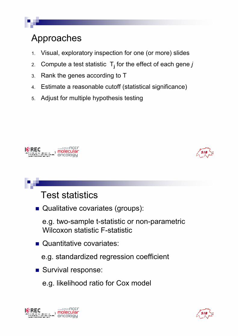
Approaches
1. Visual, exploratory inspection for one (or more) slides
2. Compute a test statistic Tj for the effect of each gene j
3. Rank the genes according to T
4. Estimate a reasonable cutoff (statistical significance)
5. Adjust for multiple hypothesis testing
4September 06
Test statistics
! Qualitative covariates (groups):
e.g. two-sample t-statistic or non-parametric
Wilcoxon statistic F-statistic
! Quantitative covariates:
e.g. standardized regression coefficient
! Survival response:
e.g. likelihood ratio for Cox model
5September 06
!
"
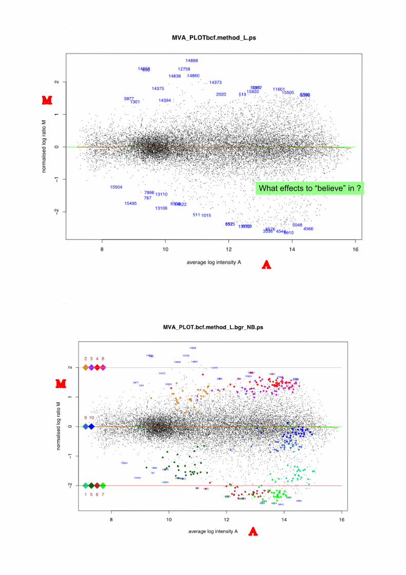
What effects to “believe” in ?
6September 06
!
"
7September 06
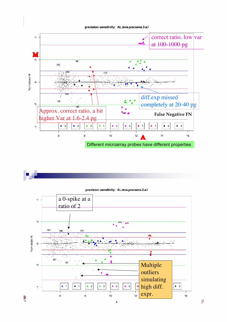
3 correct ratio, low var
at 100-1000 pg
diff.exp missed
completely at 20-40 pgApprox. correct ratio, a bit
higher Var at 1.6-2.4 pgFalse Negative FN
Different microarray probes have different properties
!
"
8September 06
a 0-spike at a
ratio of 2
Multiple
outliers
simulating
high diff.
expr.

9September 06
Single-slide methods
! Model-dependent rules for deciding whether a value pair
(R,G) corresponds to a differentially expressed gene
! Amounts to drawing two curves in the (R,G)-plane; call a gene
differentially expressed, if it falls outside the region between
the two curves
! At this time, not enough known about the systematic and
random variation within a microarray experiment to justify
these strong modeling assumptions
! n = 1 slide may not be enough (!)
10September 06
Difficulty in assigning valid p-values based on
a single slide

11September 06
Single-slide methods
! Chen et al: Each (R,G) is assumed to be normally andindependently distributed with constant CV; decision basedon R/G only (purple)
! Newton et al: Gamma-Gamma-Bernoulli hierarchical modelfor each (R,G) (yellow)
! Roberts et al: Each (R,G) is assumed to be normally andindependently distributed with variance depending linearlyon the mean
! Sapir & Churchill: Each log R/G assumed to be distributedaccording to a mixture of normal and uniform distributions;decision based on R/G only (turquoise)
12September 06
Informal methods
! If no replication (i.e. only have a single array),
there are not many options
! Common methods include:
"(log) Fold change exceeding some threshold, e.g.
more than 2 (or less than –2)
"Graphical assessment, e.g. QQ plot
! However, the threshold is pretty arbitrary
13September 06
Which genes are DE?! Difficult to judge significance
"massive multiple testing problem
"don’t know null distribution of M
"genes dependent
! Strategy
"aim to rank genes
"assume most genes are not DE (depending on typeof experiment and array)
"find genes separated from the majority
14September 06
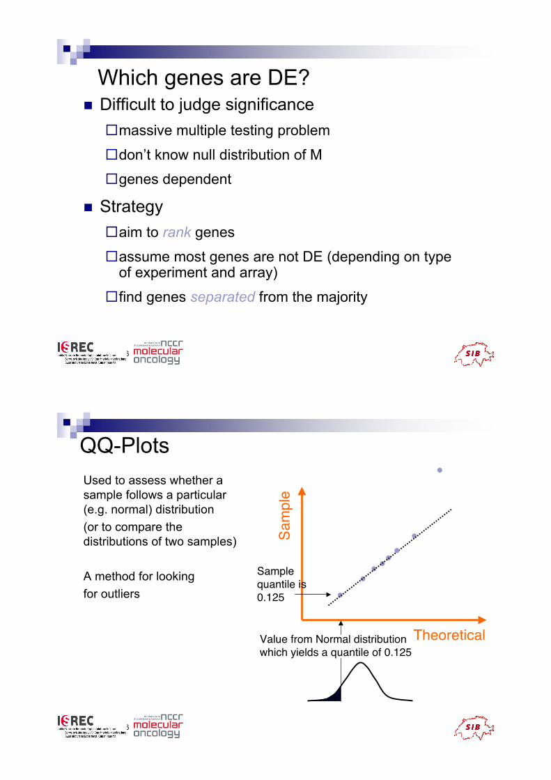
QQ-Plots
Used to assess whether a
sample follows a particular
(e.g. normal) distribution
(or to compare the
distributions of two samples)
A method for looking
for outliers
Sa
mp
le
Theoretical
Sample
quantile is
0.125
Value from Normal distribution
which yields a quantile of 0.125

15September 06
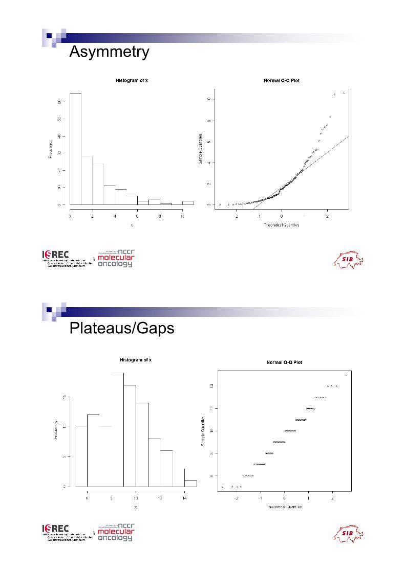
Typical deviations from straight line
patterns
! Outliers
! Curvature at both ends (long or short tails)
! Convex/concave curvature (asymmetry)
! Horizontal segments, plateaus, gaps
16September 06
Outliers

17September 06
Long Tails
18September 06
Short Tails
19September 06
Asymmetry
20September 06
Plateaus/Gaps
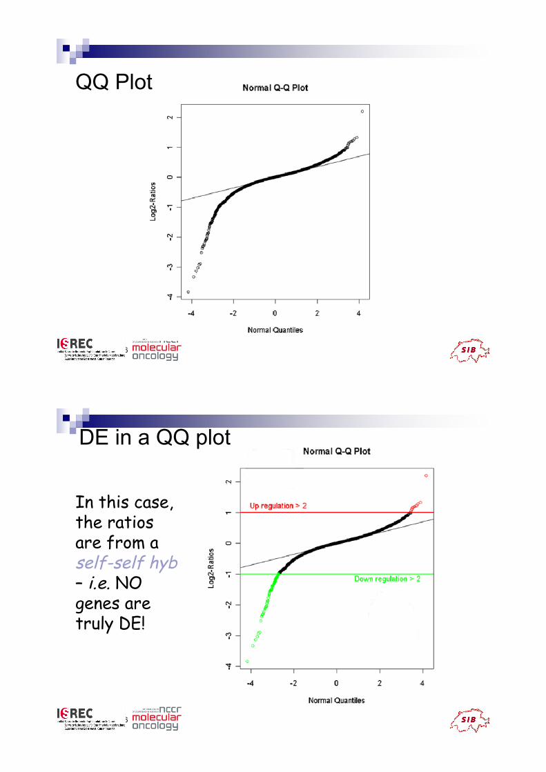
21September 06
QQ Plot
22September 06
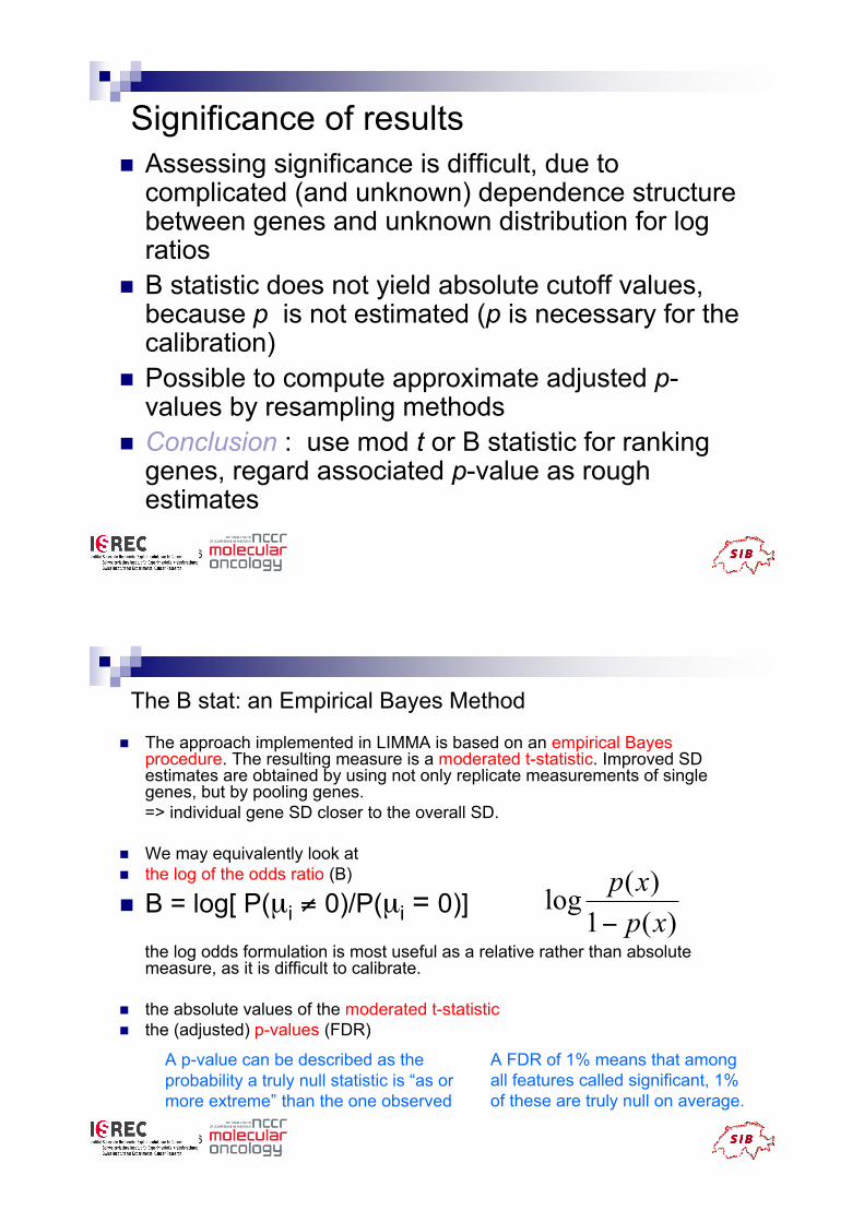
DE in a QQ plot
In this case,the ratiosare from aself-self hyb– i.e. NOgenes aretruly DE!

23September 06
Decision Table
POSITIVE CLASSIFIED AS DIFFERENTIALLY EXPRESSED
NEGATIVE CLASSIFIED AS NON DE
24September 06
Replicated experiments! Have n replicates
! For each gene, have n values of M = log2 foldchange, one from each array
! Summarize M1, ..., Mn for each gene by
"M = average (M1, ..., Mn)
"s = SD(M1, ..., Mn)
! Rank genes in order of strength of evidence infavor of DE
! How might we do this?

25September 06
Ranking criteria! Genes i = 1, ..., p
! Mi = average log2 fold change for gene i
"Problem : genes with large variability likely to beselected, even if not DE
! Fix that by taking variability into account:
use ti = Mi/ (si/#n)
"Problem : genes with extremely small variances makevery large t
" When the number of replicates is small, the smallest si
are likely to be underestimates
26September 06
G spec
T-statistics , many false positive call, when the number
of repetitions is small, y = avrg / stdev (3 repl.), x = A
true positive false positive

27September 06
G-low
y = avrg / stdev (regression estimate stdev a. A), x=A
28September 06
Shrinkage estimators
! Idea: borrow information across genes
! Here, we ‘shrink’ the ti towards zero by modifying
the si in some way (get si*)
! mod ti = ti* = Mi/(si*/#n)
ti ti* Mi
! Many ways to get a value for si*
! We will use the version implemented in theBioConductor package limma

29September 06
1: extreme in B only (B > -.5)
2: extreme in t only (|t| > 4.5)
3: extreme in B and t only
4: extreme in M only (|M| > .5)
5: extreme in M and B only
6: extreme in M and t only
7: extreme in M, B, t
Comparison of statistics
30September 06
B vs. av M
1: B only
2: t only
3: B and t only
4: M only
5: M and B only
6: M and t only
7: M, B, t

31September 06
Testing
Classical hypothesis testing is setup for a single null and alternative
hypothesis. The ’truth’ is that the null is either true or not, but we are
not able to know the truth.
Based on our collected data, we can make one of two possible
decisions: reject the null or do not reject the null. Our data cannot
tell us whether the null is true or not, only whether what we see is
consistent with the null or not.
32September 06
Testing
There are 2 types of errors we can make in this framework: we can
make the mistake of rejecting the null when it is really true (a
Type I error), or we can make the mistake of not rejecting the null
when it is really not true (a Type II error).
The Type I error is defined to be the probability, conditional on the
null being true, that the null is rejected. That is, the probability that
the test statistic falls into the rejection region. The rejection region
is determined so that the Type I error does not exceed a user-
defined rate (often 5% , but this level is not required).
One can also report a p-value, which is the probability, conditional
on the null being true, that you observe a test statistic as or more
extreme (in the direction of the alternative) than the one you got.
33September 06
Significance of results
! Assessing significance is difficult, due tocomplicated (and unknown) dependence structurebetween genes and unknown distribution for logratios
! B statistic does not yield absolute cutoff values,because p is not estimated (p is necessary for thecalibration)
! Possible to compute approximate adjusted p-values by resampling methods
! Conclusion : use mod t or B statistic for rankinggenes, regard associated p-value as roughestimates
34September 06
The B stat: an Empirical Bayes Method
! The approach implemented in LIMMA is based on an empirical Bayesprocedure. The resulting measure is a moderated t-statistic. Improved SDestimates are obtained by using not only replicate measurements of singlegenes, but by pooling genes.
=> individual gene SD closer to the overall SD.
! We may equivalently look at
! the log of the odds ratio (B)
! B = log[ P(µi $ 0)/P(µi = 0)]
the log odds formulation is most useful as a relative rather than absolutemeasure, as it is difficult to calibrate.
! the absolute values of the moderated t-statistic
! the (adjusted) p-values (FDR)
)(1
)(log
xp
xp
!
A p-value can be described as the
probability a truly null statistic is “as or
more extreme” than the one observed
A FDR of 1% means that among
all features called significant, 1%
of these are truly null on average.

35September 06
P adjusted < 0.01; B > 0.0171; |t| > 4.23
36September 06
Example: Apo AI experiment(Callow et al., Genome Research, 2000)
GOAL: Identify genes with altered expression in the livers ofone line of mice with very low HDL cholesterol levelscompared to inbred control mice
Experiment:• Apo AI knock-out mouse model
• 8 knockout (ko) mice and 8 control (ctl) mice (C57Bl/6)
• 16 hybridisations: mRNA from each of the 16 mice is labelled withCy5, pooled mRNA from control mice is labelled with Cy3
Probes: ~6,000 cDNAs, including 200 related to lipidmetabolism

37September 06
Which genes have changed?
This method can be used with replicated data:
1. For each gene and each hybridisation (8 ko + 8 ctl) use
M=log2(R/G)
2. For each gene form the t-statistic:
average of 8 ko Ms - average of 8 ctl Ms
sqrt(1/8 (SD of 8 ko Ms)2 + 1/8 (SD of 8 ctl Ms)2)
3. Form a histogram of 6,000 t values
4. Make a normal Q-Q plot; look for values “off the line”
5. Adjust for multiple testing
38September 06
Histogram & Q-Q plot
ApoA1

39September 06
Plots of t-statistics
40September 06
The multiple testing problem
! Multiplicity problem: thousands of hypotheses are tested simultaneously.
Increased chance of false positives. Choose as p-value cutoff p=0.01
! A Gene that follows the null distribution of no DE will pass the cutoff with
probability p
! Given n genes being tested, on average n*p genes will pass the cutoff. For
example n=30’000 and not a single one is differentially expressed. If the
genes would be independent, expect 300 genes wrongly called
differentially expected. Individual pvalues of e.g. 0.01 no longer correspond
to significant findings with high likelihood, many are expected even if the
set of value would have been obtained using a generator of independent
random numbers with no difference between the conditions being
compared
! This number can fluctuate strongly due to correlation between the genes. It
is not simple to base conclusions depending on the number of genes that
pass a given p-value cutoff
41September 06
Multiple Testing
In the multiple testing situation, there are several possible ways to define
an error rate which is meant to be controlled. One possibility here is the
family-wise error rate (FWER). This is the probability of at least one
Type I error among the entire family of tests.
The Bonferroni procedure is an example which provides (strong) control of
this error rate.
There is the concept of strong or weak error rate control. Weak control
only guarantees control under the complete null - ie, only if all nulls are
true. Strong control guarantees control under any combination of true
and false nulls. In the case of microarrays, it is extremely unlikely that
all nulls will be true - eg, no genes differentially expressed - so weak
control is not satisfactory in this situation.)
42September 06
Assigning unadjusted p-values to
measures of change
! Estimate p-values for each comparison (gene) by using
the permutation distribution of the t-statistics.
! For each of the possible permutation of the
trt / ctl labels, compute the two-sample t-statistics t* for
each gene.
! The unadjusted p-value for a particular gene is estimated
by the proportion of t*’s greater than the observed t in
absolute value.
8
16( ) =12,870

43September 06
Apo AI: Adjusted and unadjusted p-values for the 50 genes with the larges
absolute t-statistics
44September 06
Permutations
For paired data, permutations are obtained by switching the characteristic profiles
within each pair, yielding 2n possible permutations for n pairs of specimens.
For the unpaired or multi-group case, permutations are performed by shuffliing the
group membership labels. Note that in each case, the characteristic profiles
measured on any given specimen remain intact so as to preserve the correlation
among the measured characteristics.
With a small number of specimens, it may be possible to enumerate all possible
permutations. However, typically the number of permutations is very large, so
they are randomly sampled. For example, for paired breast tumor cases,
permutations are performed by switching with probability 1/2 the before and after
gene expression profiles within each pair.

45September 06
Type I (False Positive) Error Rates
! Family-wise Error Rate
FWER = p(FP ! 1)
! False Discovery Rate (BH)
FDR = E(FP / P) (FDR = 0 if P = 0)
! False Discovery Rate (SAM)
q-value = E(FP | H0C) / P
! False Discovery Proportion
FDP = #FP / #P (FDP = 0 if P = 0)
46September 06
FWERTraditional methods seek strong control of familywise Type I error (FWER):
The control of the error rates is strong in the sense that the error rate is
controlled regardless of which variables satisfy the null hypothesis.
If there are no effects at all, then one controls for the probability that a
hypothesis is falsely rejected. For example, Bonferroni correction
provides strong control.
The Bonferroni correction delivers an upper bound for the probability of a
type I error, that is rejection of the null hypothesis (acceptance that
there is an effect) by mistake (when there is no effect). The Bonferroni
correction is conservative.
This can be much higher than the correct p-value. This can be seen with
an extreme example. If we would (unknowingly) be measuring 1000
times the same variable and obtain the same values, the p-value would
incorrectly be estimated to be 1000 times higher than its actual value.

47September 06
Control of the FWER! Bonferroni single-step adjusted p-values
pj* = min (mpj, 1)
! Take into account the joint distribution of the test statistics:
! Westfall & Young (1993) step-down minP adjusted p-values
! Westfall & Young (1993) step-down maxT adjusted p-values
! Step-down procedures: successively smaller adjustments
at each step, Less conservative than Bonferroni
48September 06
Stepwise Procedures
The Bonferroni procedure is an example of a single step procedure - it
applies an equivalent p-value correction based on the total number of
hypotheses, regardless of the ordering of the unadjusted p-values.
It has long been recognized that stepwise (sequential) procedures can
proved more power while maintaining error rate control.
Stepwise procedures (step-down or step-up) allow each p-value to have
its own individual correction, which is based not only on the number of
hypotheses but also on the outcomes of the other hypothesis tests.
Stepwise procedures start with the unadjusted p-values ordered either
from most significant to least significant (the step-down order) or from
least significant to most significant (the step-up order). p-values are
then successively adjusted, with the adjustment depending on the
outcome of the previous tests.

49September 06
Other Proposals
While numerous methods were available for controlling the family-wise type I error
rate (FWE), the multiplicity problem in microarray data does not require a
protection against even a single type I error, so that the severe loss of power
involved in such protection is not justified.
Instead, it may be more appropriate to emphasize the proportion of errors among
the identified differentially expressed genes. The expectation of this proportion is
the false discovery rate (FDR).
Korn et al. proposed two stepwise permutation-based procedures to control with
specified confidence the actual number of false discoveries and approximately
the actual proportion of false discoveries rather than the expected number and
proportion of false discoveries.
Simulation studies demonstrate gain in sensitivity (power) to detect truly
differentially expressed genes even when allowing as few as one or two false
discoveries.
Application of the methods allows statements such as “with 95% confidence, the
number of false discoveries does not exceed 2 or with approximate 95%
confidence, the proportion of false discoveries does not exceed 0.10”.
50September 06
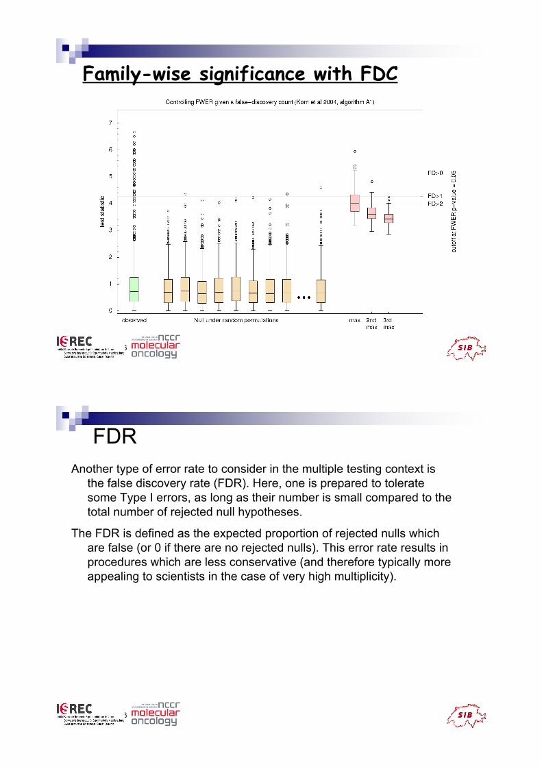
Assessing significance under multiple
testing via permutations, Korn’s method
! Estimate p-values for each comparison (gene) by using
the permutation distribution of the rank-specific t-statistics.
! For each of the possible permutation of the
trt / ctl labels, compute the two-sample t-statistics t* for
each gene. Compute the distributions of the rank k highest
statistics t*(k) from each permutation.
! The p-value for false discovery count = k for a the gene is
estimated by the proportion of t*(k) greater than the
observed t in absolute value.
8
16( ) =12,870
51September 06
Family-wise significance with FDC
52September 06
FDR
Another type of error rate to consider in the multiple testing context is
the false discovery rate (FDR). Here, one is prepared to tolerate
some Type I errors, as long as their number is small compared to the
total number of rejected null hypotheses.
The FDR is defined as the expected proportion of rejected nulls which
are false (or 0 if there are no rejected nulls). This error rate results in
procedures which are less conservative (and therefore typically more
appealing to scientists in the case of very high multiplicity).
53September 06
Control of the FDR
realized False Discovery Rate FDR = FP / P
! Benjamini & Hochberg (1995): step-up procedure which controls the
expected FDR under some dependency structures
! Benjamini & Yuketieli (2001): conservative step-up procedure which
controls the expected FDR under general dependency structures
! ‘Significance Analysis of Microarrays (SAM)’ q value (2 versions)
" Efron et al. (2000): weak control
" Tusher et al. (2001): strong control
! ‘Korn’s method’ controls for the false discovery counts and
approximately controls the FDR
" Korn et al. (2003, 2004):
54September 06
Benjamini & HochbergThe BH procedure is a step-up procedure that provides strong control of the FDR.
The key to understanding/interpretation is to understand the meaning of the FDR.
The FDR indicates the expected (average) proportion of ’discoveries’ (ie, rejected
null hypotheses) that are ’false discoveries’ (ie, the null is really true). A rejected
null corresponds to a gene identified by the test as ’interesting’, while a true null
represents genes that are in reality biologically ’uninteresting’.
This means that if the BH adjusted p-value is .05 (say), then for every 20 rejected
nulls (’interesting’ genes) you expect 1 of those in fact to correspond to a true null
(’uninteresting’ genes). Because the error rate control applies to what should
happen ’on average’, the actual number of false discoveries per 20 rejected nulls
may be larger or smaller than 1.
Also, we cannot tell just based on the FDR which of the rejected nulls are the false
discoveries. One way to use the FDR is to prioritize genes for further follow-up. If
there are no genes with small FDR, then you should be prepared for several of
the ’discoveries’ not to hold up under further scrutiny. If the FDR for a gene is too
big, it may be decided to concentrate resources on other genes, or other types of
experiments.

55September 06
Benjamini & Hochberg
Can power be improved while maintaining control over a meaningful
measure of error?
Benjamini & Hochberg (1995) define a sequential p-value procedure that
controls expected FDR FP/P. Specifically, the BH procedure guarantees
E (FDR) " F / M * % " % .
That is that for a pre-specifed 0 < % < 1, a cutoff is given at which the
expected FDR is not superior to the desired value.
Benjamini and Hochberg advocated that the FDR should be controlled at
some desirable level, while maximizing the number of discoveries made.
They offered the linear step-up procedure as a simple and general
procedure that controls the FDR. The linear step-up procedure only makes
use of the m p-values, P = (P1, ..., Pm) so it can be applied to any statistics
that yields (single test) p values.
56September 06
FDR estimation by SAM

57September 06
R / BioConductor! limma differential expression for designed
experiments, moderated t and B statistics, FDR
http://bioinf.wehi.edu.au/limma/
http://bioinf.wehi.edu.au/limmaGUI/
! samr SAM methods for differential expression and
q value (older: siggenes)
http://www-stat.stanford.edu/~tibs/SAM/index.html
! multtest adjustments for multiple hypotheses
58September 06
Acknoledgements
! Slides and Text contributions by
! Darlene Goldstein
! Terry Speed
! Asa Wirapati
! Members of the BCF
Recommended