Discrete dipole model of radiative transfer in dense granular layers
Sanaz Vahidinia12 Jeffrey N Cuzzi2 Bruce Draine3 Essam Marouf4
1Corresponding author NASA Postdoctoral Associate 2Space Science Division Ames Reshy
search Center NASA 3Astronomy Department Princeton University 4Electrical Engineershy
ing Department San Jose State University
We have developed a numerical Regolith Radiative Transfer (RRT) model
based on the Discrete-Dipole Approximation (DDA) which iteratively solves
the exact wave equations for a granular target in response to an incident plane
wave and mutual interactions between all component grains We extend the
traditional DDA approach in two ways the DDA target is laterally replicated
using periodic boundary conditions to represent a small piece of a nominally
flat granular particle surface and the emergent intensity is sampled in the
near field of the target to avoid diffraction-like artifacts arising from its finite
size The approach is applicable in regimes for which the assumptions of
current RRT models are invalid such as wavelength-size particles which are
closely packed In this first paper we describe the technique and present tests
and illustrative results for simple cases using layers of varying filling fraction
between 001 and 07 containing nominally spherical monomers of uniform
composition (SiO2) We motivate the results with a simple ldquotoy modelrdquo of
scattering by a target with multiple interfaces The model is easily extended
to layers of particles which are heterogeneous in composition and arbitrarily
shaped copyc 2017 Optical Society of America
1 Introduction
Interpreting remote observations of granular bodies is an important tool in determining the
surface composition of all airless solid bodies in the solar system The granular surfaces of
these bodies are constantly fragmented and mixed by meteoroid impacts and are referred
to as regoliths Regolith particles are often comparable to or smaller than the wavelength of
interest and are packed to varying degrees of porosity such that many particles are touching
Models by Conel (1969) Hapke (eg 1981 1983 1999) Lumme and Bowell (1981) Shkushy
ratov et al (1999ab) and others have had many successes but make certain simplifying
assumptions which are not valid in all regimes of interest and consequently fail to match the
appearance of the spectra of granular materials at certain wavelengths (Moersch and Chrisshy
tensen 1995 see also section 2 below) All widely used models are suspect when the grains
1
are not well-separated but indeed closely packed violating the assumptions of independent
particle scattering (see however Mishchenko 1994 Mishchenko and Macke 1997 Pitman et
al 2005) and HapkeShkuratov models in particular become problematic when the regolith
grains are not large compared to a wavelength As the expectations of compositional deshy
termination by remote sensing and in particular by thermal infrared spectroscopy become
more demanding improved theories will be needed which are able to at least adequately
represent the spectral properties of known samples This calls for a theory that reproduces
the spectra of known samples over a wide range of refractive indices sizewavelength ratio
and porosity
Modeling a regolith layer generally starts with calculating the single scattering properties
(albedo and phase function) of an individual regolith grain and then using one of several
methods to derive the overall reflection and transmission of a semi-infinite layer composed
of many similar grains The approaches to date have been adapted from classical approaches
to atmospheric radiative transfer In clouds for instance individual scatterers are generally
separated by many times their own size and the scattering behavior of an isolated particle
is appropriate for modeling ensembles of these particles The single scattering albedo can be
calculated analytically for small particles in the Rayleigh limit and Mie scattering is used
for larger spherical particles Semi-empirical adjustments can be made at this stage to allow
for particle nonsphericity (Pollack and Cuzzi 1979) or more elaborate T-matrix calculations
can be used (Waterman 1965 Mishckenko et al 1996) Mie scattering is cumbersome in the
geometrical optics limit but various ray-optics based approaches can be used here (Shkuratov
1999ab Mishchenko and Macke 1997 Hapke 1999)
Once the grain single scattering albedo wo and scattering phase function P (Θ) (the disshy
tribution of intensity with scattering angle Θ from the incident beam) are obtained various
multiple scattering techniques can be used to derive the properties of an ensemble of such
particles in a layer These techniques include the N-stream or discrete ordinates approach
(Conel 1969) addingdoubling of thin layers (Hansen and Travis 1974 Wiscombe 1975(ab)
Plass 1973) or Chandrasekharrsquos XY or H functions for which tabulations and closed-form
approximations exist in the case of isotropic scattering (Hapke 1981) A variety of ldquosimilarshy
ity transformationsrdquo can be used to convert arbitrary grain anisotropic scattering properties
into their isotropic scattering equivalents (van de Hulst 1980 see Irvine 1975) allowing the
use of these standard isotropic solutions
Generally these approaches assume the regolith grains have scattering properties which
can be calculated in isolation The independent scattering assumption is normally assumed
to be satisfied when the particle spacing l is larger than several grain radii rg (van de
Hulst 1981)1 Hapke (2008) has extended this spacing constraint to be a function of the
1The source is a brief comment in section 121 of van de Hulstrsquos book
2
radiuswavelength ratio itself by adopting van de Hulstrsquos assertion about the required spacshy
ing and interpreting this spacing as a distance between surfaces of adjacent particles This
approach predicts that interference effects are not important in most regoliths when rg raquo λ
but filling factors less than 01 are needed to validate incoherent independent scattering
when rg sim λ (see Appendix A)
A number of theoretical and experimental studies have been conducted regarding the role
of close packing effects for over fifty years An early study found changes in reflectance with
porosity depended on grain albedo (Blevin and Brown 1961) Some studies have concentrated
on the dependence of extinction on porosity without discussing the scattering or reflectivity
of the medium (Ishimaru and Kuga 1982 Edgar et al 2006 Gobel et al 1995) these latter
studies are valuable in indicating the porosity regime where packing effects become important
(around 10 volume filling factor) but even this threshold is a function of particle size and
wavelength (Ishimaru and Kuga 1982) As a partial attack on the close-packing problem
various approaches have been tried to treating the diffracted component of both the phase
function and albedo as unscattered in the dense regolith environment (Wald 1994 Pitman
et al 2005 see however Mishchenko 1994 and Mishchenko and Macke 1997 for cautionary
notes) Other research has focussed on the Lorentz-Lorentz (EMT or Garnett) technique
for fine powders and variants on hard-sphere packing positional correlation functions such
as the Percus-Yevick static structure theory (Mishchenko 1994 Pitman et al 2005) These
approaches are promising in some ways but in other ways they degrade agreement with the
data (Pitman et al 2005)
Few of these studies to date have attempted a combined treatment of variable refractive
indices and porosity but it is precisely this combination that leads to some of the most
glaring failures of traditional models (see below) The formulation by Hapke (2008) suggests
that increased filling factor almost always leads to increased reflectivity unless the scattering
grains have extremely high albedo wo gt 095 Indeed Blevin and Brown (1961) find that
packing increases the reflectance of dark materials and decreases that of bright materials
however the grain albedo threshold where the behavior changes may not be as high as
modeled by Hapke (2008) Finally many previous studies apply to regimes where the particle
size is large compared to the wavelength
Our approach can capture the combined role of sizewavelength (even when they are comshy
parable) porosity and refractive index It avoids all of the common but frequently inapproshy
priate simplifying assumptions by use of the discrete dipole approximation (DDA) to model
radiative transfer in granular regoliths In the DDA scattering calculations are not limited
by packing density shape or size of particles in the regolith The technique has become more
productive since its introduction (Purcell and Pennypacker 1973) due to a combination of
increasing compute power and improved algorithms (Draine and Flatau 2004 2008) comshy
3
putational power remains its limiting factor however In section 2 we compare predictions of
some current models with spectral data to illustrate shortcomings of the models In section
3 we describe our model which has several novel aspects In sections 4 and 5 we present
some tests In section 6 we give some preliminary results and in section 7 give possible
explanations and speculations
2 Current model inadequacy Thermal emission spectroscopy of SiO2
Thermal emission spectroscopy is central to a new generation of planetary and astronomical
exploration moreover it lies entirely in the problematic regime where the regolith grain
size and separation are both comparable to the wavelength Like nearly all treatments in
the past our models of emission spectroscopy start with reflectivities R and relate them to
emissivities E by the principle of detailed balance or Kirkhoffrsquos law (Goody 1964 Linsky
1972) in the simplest case when both quantities are integrated over all incident and emergent
angles E = 1 minus R Analogous expressions can be derived when angle-dependent quantities
are needed (see below)
Regolith scattering by grainy surfaces can be categorized by two or three major optical
regimes defined by the refractive indices of the regolith material (see Mustard and Hays 1997
for a review) The first spectral regime is called ldquosurface scatteringrdquo (at wavelengths where
real andor imaginary refractive indices and surface reflectance are large and the wave
hardly penetrates into the material) restrahlen bands fall in this regime The second regime
is ldquovolume scatteringrdquo (at wavelengths where the imaginary index is low and the real index
is of order unity) which has a more moderate surface reflectivity transparency regions result
from this range of properties (Mustard and Hays 1997 MH97) Increasing the imaginary
index in this refractive index regime increases absorption and decreases reflectivity A third
characteristic spectral property is a Christiansen feature where the real index is equal to 1 so
surface reflections vanish and the emissivity closely approaches unity Mineral identification
and grain size estimation from remote sensing data follow from modeling the shapes and
relative strengths of these strong and weak spectral features
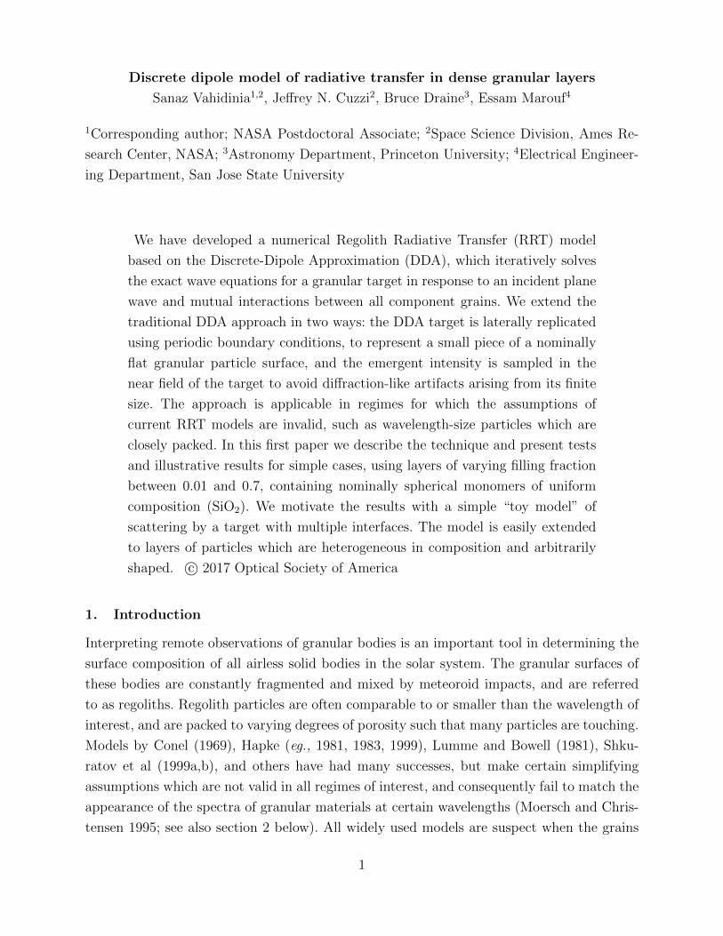
As an exercise complementary to that of Moersch and Christensen (1995) we compared the
performance of several typical RRT models against new laboratory measurements of thermal
emissivity from layers of quartz grains with various sizes (data courtesy P Christensen
and J Michalski) The data were taken at room temperature and represent directional
emissivities viewed roughly 30 degrees from the normal with a field of view 30 degrees
wide Regolith samples were approximately 1 cm thick and their porosity is estimated by
weighing as approximately 30 (P Christensen personal communication 2011) Our models
used recent values of SiO2 refractive indices from Wenrich and Christensen (1996) who (as
did MC95) noted a discrepancy with the standard values of Spitzer and Kleinman (the
4
discrepancy apparently arises from tabulated values of oscillator parameters in Spitzer and
Kleinman) In any case we find that the differences in refractive indices - perhaps at the
10 level at the lowest values of imaginary index in transparency bands - have only a barely
noticeable effect on the model results shown in figure 1 Since the SiO2 refractive indices
have now been measured twice independently with the differences having a negligible effect
on model results this suggests that the model-data discrepancies in the transparency bands
are not due to uncertainties in SiO2 refractive indices but arise from a more profound cause
Our three models are similar to those used by MC95 (one is identical) and will be seen to
capture the same general behavior All of our models used Mie theory to get the individual
grain albedo wo phase function Po(Θ) and asymmetry parameter go directly from the reshy
fractive indices This is because the first step of Hapke theory (using geometrical optics to
get the grain albedo) is not justifiable here where the grain size and wavelength are compashy
rable The asymmetry parameter go = (cosΘ) is a mean of (cosΘ) over scattering angle Θ
as weighted by the phase function (see the review by Irvine 1975) To allow for the optical
anisotropy of SiO2 we computed grain properties separately using the ordinary (ord) and
extraordinary (ext) ray refractive indices and then obtained weighted grain averages using
wo = (2woord + woext)3 and similarly for go
Mie theory implicitly includes diffraction in wo Po(Θ) and go because the particles are
treated as isolated independent scatterers and for nearly all combinations of grain radius
and wavelength regolith grains are substantially forward scattering (see Hansen and Travis
1974 or Mishchenko and Macke 1997) Two of our models accept this behavior at face value
Both then obtain thick-layer solutions using very similar scaling relations In one of the
earliest attacks on this problem Conel (1969) showed that a simple two-stream solution to
the radiative transfer equation taken to the limit of a semi-infinite layer has a closed-form
solution for hemispherical (flux) reflectivity R and emissivity E = 1 minus R
2 E = 1 minus R = where (1)
u minus 1 121 minus wogo u = (2)
1 minus wo
MC95 present plots of results using this theory although note a typo in the equation just
below their equation 9 (compare Conel 1969 equations 10 and 15) our results for this and
other models are shown in figure 1
In our second model we use an empirical scaling transformation from van de Hulst (1980)
which also starts with wo and go and derives a more detailed scaling relation for the inteshy
grated spherical albedo A of a large smooth regolith-covered particle which is close to the
hemispherical reflectivity R of a slab of its surface (see Cuzzi 1985)
(1 minus s)(1 minus 0139s)E = 1 minus R = 1 minus where (3)
1 + 117s
5
121 minus wo 1
s = = (4)1 minus wogo u
The van de Hulst expression for E (equation 3) is basically a numerical refinement of Conelrsquos
two-stream expression (based on many comparisons with exact calculations) expanded to
higher order in s in that the van de Hulst R sim (1 minus s)(1 + s) = (u minus 1)(u + 1) which is
exactly the Conel R so it is not entirely independent but does enjoy some independent and
exhaustive numerical validation
In Hapke theory the diffraction lobe of the grain is explicitly neglected to motivate
isotropic scattering which is then assumed for all orders of scattering except the first (for
isotropic scattering the H-functions of Chandrasekhar are readily available) The validity of
retaining or removing the diffraction contribution to the grain albedo and phase function has
been debated in the literature (see Wald 1994 Wald and Salisbury 1995 Mishchenko and
Macke 1997 and Pitman et al 2005) In fact even if the diffraction lobe per se is arbitrarily
removed this does not necessarily imply the remainder of the scattering by the grain is
isotropic (Pollack and Cuzzi 1979 Mishchenko and Macke 1997) However for illustrating
the state of widely used models we include in figure 1 an H-function based emissivity as
a placeholder for the full Hapke theory Since we use Mie scattering to obtain wo and go
we transform these values to equivalent isotropic scattering albedos wi using a standard
similarity transformation (Irvine 1975 and Hapke 1983 equation 1025a)
wo(1 minus go) wi = (5)
1 minus wogo
For forward scattering particles this transformation reduces the albedo and can be thought
of as ldquotruncatingrdquo or removing the diffraction peak We then proceed to integrate the bidishy
rectional reflectivity R(microo micro) which is a function of incidence angle θo and emission angle
θ where microo = cosθo and micro = cosθ (Chandrasekhar 1960)
wi microoR(microo micro) = H(microo)H(micro) (6)
4π microo + micro
over all incidence angles θo to derive the normal (hemispherical-directional) reflectivity R(micro =
1) using closed form expressions for H in Hapke 1983 (equations 822b 825 and 857) and
then set the corresponding emissivity E(micro = 1) = 1 minus R(micro = 1) (Goody 1964 Linsky 1972)
While the Mie-Conel and Mie-van de Hulst models are in the spirit of hemispherical emisshy
sivities (averaged over viewing angle) the Mie-H-function model is a directional emissivity
(at normal viewing) As the experimental data used a beam of significant angular width it
is not clear whether either of these is to be preferred a priori The Mie-Conel and Mie-van
de Hulst approaches accept the forward-scattering nature of the grains as calculated by Mie
theory and the Hminusfunction (and Hapke) models effectively preclude it Pitman et al (2005)
6
used a discrete ordinates code rather than assuming isotropic scattering and also found
similar behavior before applying their packing corrections
Fig 1 Comparison of Mie-Conel Mie-van De Hulst and Mie-H-function models (dotted
dot-dashed and dashed lines) with laboratory emissivity measurements of layers of size-
sorted granular quartz (solid lines J Michalski and P Christensen personal communication
2006) for three separate grain sizes
For the largest grain sizes our models and previous models are in fair agreement with the
experimental data However for wavelength-sized and smaller grains the correspondence is
unsatisfactory as already shown by Moersch and Christensen (1995 MC95) Mustard and
7
Hays (1997 MH97) and Pitman et al (2005) for grains with a well known size distribushy
tion For quartz MH97 and MC95 both find that strong restrahlen bands show almost
no variation with regolith grain size while the data show noticeable variation These are
the high-refractive-index ldquosurface scatteringrdquo regimes Even bigger discrepancies are seen in
the ldquovolume scatteringrdquo transparency regimes For moderate-size grains the models predict
emissivity minima in transparency bands such as 10-12microm 13-145microm and 15-17micromwhich
are much more dramatic than shown by the data and the discrepancy increases with smaller
grain size (also pointed out by Wald and Salisbury 1995) MH97 even show (in their figure
11) that the sense of the observed 10-12 and 13-14microm band strength variation as grain
size varies between 2-25microm is directly opposite the sense predicted by the models in figure
1 In the spectral range 19-225microm the models predict a double minimum in the emissivshy
ity while the data show a single minimum This might be related in some way to how all
these models treat the birefringence properties of SiO2 Furthermore MH97 show that the
asymmetry of the restrahlen bands for Olivine at 9-11microm wavelength is opposite that of theshy
oretical predictions For SiO2 our model results reinforce these conclusions Hapke (2008)
suggested that for almost all cases except extremely high grain albedos increased (realistic)
volume filling factor increases reflectivity However as we see from comparing ideal models
to nonideal data the data show increased emissivity (decreased reflectivity) in transparency
regions relative to the models As we show models which both include and reject grain
forward scattering this alone is unlikely to be the primary reason (although the Hminusfunction
model which rejects forward scattering and forces the phase function to be isotropic might
be said to provide marginally better agreement with the data) Thus we feel that a good
explanation for the observed effects is still to be found
It is perhaps not surprising that current models have such problems because their basic
assumptions (widely spaced and independently scattering particles which are either spherical
(Mie) much larger than the wavelength andor independently scattering are violated by key
physical properties of regolith surfaces in the regime shown (close packing irregular particles
wavelength size grains) The fact that these popular models fail to capture important features
of laboratory silicate data casts doubt on their validity for inferences of grain composition or
size from mid-infrared observations of planetary surfaces in general As discussed below we
suspect the primary explanation for the discrepancy is the effect of the nonideal (moderate
to large) volume filling factor of the real granular material
3 A new RRT model using the Discrete Dipole Approximation
Our model is based on the Discrete Dipole Approximation (DDA) which calculates the scatshy
tering and absorption of electromagnetic waves by a target object of arbitrary structure - in
our case for closely packed irregular grains of arbitrary radius rg Target objects are modshy
8
eled with a suitably populated lattice of individual polarizable dipoles with size smaller than
a wavelength The polarizability of each dipole can be adjusted to represent the refractive
index of an arbitrary material or free space (Draine and Flatau 19941988) An important
criterion for the dipole lattice is that the size of and spacing between the dipoles (both given
by d) must be small compared with the wavelength λ = 2πk of the incident radiation in the
target material |M |kd lt 12 where M is the complex refractive index of the target The
second criterion is that for a given d the total number of dipoles N must be large enough
to resolve the internal structure of the target and its constituent monomers satisfactorily
In our case monomers may overlap but typically we need (rgd)3 dipoles per monomer
Heterogeneous composition and irregular shape of monomers are easily captured this way
but we reserve those refinements for the future
To apply the DDA approach to a regolith layer we have made several changes from the
traditional implementation In one novel modification horizontally extended semi-infinite
slabs of regolith made up of closely packed grains of arbitrary size and shape are modeled
using a single target ldquounit cellrdquo subject to periodic horizontal boundary conditions or PBC
(Draine and Flatau 2008) In a second novel modification the emergent intensities from the
layer are calculated using the full near field solution traditionally all scattering calculations
have been done in the far field This step itself has two parts evaluating the scattered elecshy
tric field on a planar 2-D grid close to the target cell and evaluating the angular intensity
distribution emerging from this grid in an outbound hemisphere using a Fourier transform
approach These angular distributions of emergent intensity which can be sampled on Gausshy
sian quadrature grids can then provide input into standard adding-doubling codes to build
up solutions for thicker layers than we can model directly with DDA this next step is a
subject for a future paper
Below we describe our approach in its three main elements (A) horizontal periodic boundshy
ary conditions (B) calculation of the scattered fields in the near field of the target and (C)
determination of the angular distribution of the emitted radiation using a Fourier analysis
ldquoangular spectrumrdquo method
3A Periodic boundary conditions
A finite rectangular slab of monomers composed of gridded dipoles referred to as the Target
Unit Cell (TUC) is periodically replicated to represent a horizontally semi-infinite 3-D layer
(see Draine and Flatau 2008) Each dipole in the TUC has an image dipole in each periodic
replica cell All dipoles in the TUC and replica oscillate with the appropriate phases in their
initial response to an incident plane wave The electromagnetic field inside the target is then
recalculated as the sum of the initial radiation and the field from all other dipoles in the
layer monomers on the edge of the TUC are still embedded in the field of many adjacent
9
monomers by virtue of the PBC A steady state solution is obtained by iterating these steps
The dipoles are located at positions r = rjmn with the indices m n running over the replica
targets and j running over the dipoles in the TUC
rjmn = rj00 + mLyy + nLz z (7)
where Ly Lz are the lengths of the TUC in each dimension The incident E field is
ikmiddotrminusiwt Einc = E0e (8)
The initial polarizations of the image dipoles Pjmn are also driven by the incident field
merely phase shifted relative to the TUC dipole polarization Pj00
ikmiddot(rj00+mLy y+nLz z)minusiwt ik(rjmnminusrj00)Pjmn = αjEinc(rj t) = αj E0e = Pj00e (9)
The scattered field at position j in the TUC (m = n = 0) is due to all dipoles both in the
TUC (index l) and in the replica cells ik(rjmnminusrj00) ik(rjmnminusrj00)Pl00 equiv minusAP BC Ej00 = minusAjlmn Pl00e = minusAjlmne jl Pl00 (10)
AP BC is a 3 x 3 matrix that defines the interaction of all dipoles in the TUC and replicas jl
residing in the periodic layer (Draine 1994 2008) Once the matrix AP BC has been calculated jl
then the polarization Pj00 for each dipole in the TUC can be calculated using an iterative
technique AP BC Pj00 = αj Einc(rj ) minus jl Pl00 (11)
l
where the criterion for convergence can be set by the user In the next two subsections we
will show how we go from the field sampled on a two dimensional grid parallel to the target
layer to a full three dimensional angular distribution in elevation and azimuth relative to
the target layer normal
3B Calculating radiation from the PBC dipole layer
Once a converged polarization has been obtained for all dipoles in the target layer we can
calculate the radiated field For most purposes in the past the radiated field was calculated
in the far field of the target (kr raquo 1) however this introduces edge effects inconsistent
with a laterally infinite horizontal layer since the radiation is calculated by summing over
the radiated contributions only from a single TUC (see Appendix B) This problem would
remain even if we were to include more image cells or a larger TUC no matter how large the
target its finite size will be manifested in the far radiation field as an increasingly narrow
diffraction-like feature Another consideration supporting the use of the near field is that we
10
Y I bull bull -i)middot middot
Fig 2 Schematic of the DDA code operated in the Periodic Boundary Conshy
dition (PBC) regime with the Target Unit Cell (TUC) shown in the center
and image cells arrayed around Io indicates an incident plane wave ( flux in
erg cmminus2 secminus1) and Is indicates the scattered flux Θ (and θ) are the angles
between the incident (and scattered) beam and the a1 axis normal to the parshy
ticle layer Also φo and φ are the azimuth angles of these beams around the
normal of the layer The angle β determines the azimuth angle of the incident
beam relative to the a3 axis fixed to the target The phase angle of the scatshy
tered beam is α and the scattering angle of the emergent beam relative to the
incident beam is θs
11
plan to build up the properties of thick targets beyond the computational limits of the DDA
by combining the properties of our DDA targets using an adding-doubling approach in which
each is envisioned to be emplaced immediately adjacent to the next For this application the
far field limit does not apply and we have to move closer to the layer to sample the radiation
field
3B1 The near field
Our solution to the problems mentioned above is to calculate the radiated field in close
proximity of the target that is in its near field In the forward direction this region can be
thought of as the shadow of the layer We use the full free space Greenrsquos function which
incorporates all proximity effects to calculate the radiated field in this regime The radiated
field is a sensitive function of position with respect to the layer In the horizontal (y and z)
directions the phase of the field fluctuates rapidly In the x direction as the field travels
away from the layer it transitions from the true near field (where evanescent waves can
be present) to the Fresnel zone where patches of dipoles within the target are oscillating
coherently and finally to the far field limit where the layer is seen as a finite target
Fig 3 Schematic of our approach illustrating how we obtain the forward
scattered diffuse intensity at point X in the shadow or Fresnel zone of the
TUC uncorrupted by edge effects from the TUC (see Appendix B) The diffuse
reflectivity is determined at a similar distance from the lit face of the TUC
12
3B2 Sampling the field on a 2-D sheet
The first step in obtaining the scattered intensity within the classical shadow zone of the slab
is to calculate the total electric field on a 2-D grid (which we call the Target Unit Radiance
or TUR) just outside the layer We will use both the TUC and the image cells out to some
distance in calculating the field on the TUR The general expression for the field due to a
collection of j dipoles with polarization Pj is as follows
N ETUR = k2 Pj middot G where (12)
j=1
ikrjke ikrjk minus 1G = k2(rjkrjk minusI) +
2 (3rjkrjk minusI) (13)
rjk rjk
where rj = distance to grid points in the TUC rk = distance to grid points in the TUR rjk = |rj minus rk| rjk = (rj minus rk)rjk I is the identity tensor and G is the free
space tensor Greenrsquos function The field is calculated on TURrsquos on both sides of the
slab ie on the reflected and transmitted sides The transmitted side includes both
the directly transmitted incident electric field that has been attenuated through the slab
and the scattered field This method has been written as a FORTRAN code called
DDFIELD one version of which is currently distributed with DDSCAT as a subroutine
(httpwwwastroprincetonedu draineDDSCAThtml) The version used in this paper is
slightly different and was parallelized using MPI and OpenMP The dipole polarizabilities
calculated by DDSCAT are fed into DDFIELD to calculate the electric field from them The
vector field E(y z) = Ex(y z)x + Ey(y z)y + Ez(y z)z is calculated separately for each of
the two polarization states of the incident radiation
3C Determining the angular distribution of scattered intensity
Our approach to determining the emergent intensities in the near field as a function of angle
(θ φ) for any given (θo φo) follows the formalism of Mandel and Wolf (1994) A complex field
distribution or waveform can be represented by a superposition of simple plane waves and
Fourier decomposed across a plane (see below) The waveforms spatial frequency components
represent plane waves traveling away from the plane in various angular directions Consider
a monochromatic wave-field E(x y z) that satisfies the Helmholtz equation across the TUR
plane at x = x0 it can be represented by a Fourier integral ETUR = E(x0 y z) = E(x0 ky kz)e i(ky y+kz z)dkydkz (14)
Then the field E(x0 y z) has the following inverse transform E(x0 ky kz) = E(x0 y z)e minusi(ky y+kz z)dydz (15)
13
The Helmholtz equation is
(2 + k2)E(r) = 0 where r = (x y z) (16)
Substituting the 2-D representation of the field E(x y z) into the Helmholtz equation we
get the differential equation
part2E(x0 y z) + kx
2E(x0 y z) = 0 (17)partx2
with the general solution
ikxx0 minusikxx0E(x0 ky kz) = A(ky kz)e + B(ky kz)e (18)
In addition we assume 2π
k2 = k2 minus k2 minus k2 k = (19)x y z λ
kx = (k2 minus ky 2 minus kz
2) 1 2 where ky
2 + kz 2 le k2 or (20)
kx = i(ky 2 + kz
2 minus k2) 2 1
where ky 2 + kz
2 gt k2 (21)
Because the roots with ky 2 + kz
2 gt k2 are evanescent and will decay rapidly away from the
layer we will sample the field at a position x0 where the evanescent terms have decayed
and are negligible (as determined by tests) We would like to compute the scattered field
emanating away from the target therefore we will only consider the solution in a half space
in the reflected region x lt 0 B(ky kz) = 0 (equation 18) and in the transmitted region x gt 0
A(ky kz) = 0 We can proceed with the development using one side since the other differs
by a minus sign For example on the transmitted side we can write the Fourier transform of
the electric field across any plane x = x0 as follows
ikxx0A(ky kz)e = E(x0 y z)e i(ky y+kz z)dkydkz (22)
where the scattered electric field E(x0 y z) has been computed on a grid of points on a plane
x = x0 in the shadow zone (the TUR) The Fourier transform of the electric field on the
TUR gives the relative strength of each spatial frequency component A(ky kz) composing
that field and therefore of each plane wave stream leaving the TUR The distribution of
energy as a function of spatial frequency k = 2πλ should be highly localized at k2 allowing
us to determine k2 = k2 minus k2 minus k2 Its angular distribution is the angular distribution of x y z
the emergent scattered intensity at the plane x = x0 Because the components A(ky kz) are
formally fluxes we must transform them into intensities (see section 3C1) This approach
will also provide a way to discriminate against any static components in the field appearance
of significant anomalous energy at high spatial frequencies (ie much higher than |k|) is an
indication of static evanescent fields If this problem were to appear (it has not yet with
x0 sim λ) we would merely move the TUR slightly further from the face of the TUC
14
3C1 Flux and Intensity
The discrete transform quantities Ai(ky kx) with i = x y z represent components of plane
waves with some unpolarized total flux density
|Ai(θ φ)|2 (23) i=xyz
propagating in the directions θ(ky kz) φ(ky kz) where the angles of the emergent rays are
defined relative to the normal to the target layer and the incident ray direction (θ0 φ0)
kx = kcosθ (24)
ky = ksinθsin(φ minus φ0) (25)
kz = ksinθcos(φ minus φ0) (26)
where k = 1λ and we solve at each (ky kz) for kx = (k2 minus ky 2 minus kz
2)12 It is thus an
implicit assumption that all propagating waves have wavenumber k = 1λ we have verified
numerically that there is no energy at wavenumbers gt k as might occur if the the DDFIELD
sampling layer at xo had been placed too close to the scattering layer
From this point on we assume fluxes are summed over their components i and suppress
the subscript i The next step is converting the angular distribution of plane waves or
flux densities (energytimearea) |A(ky kz)|2 into intensities (energytimeareasolid anshy
gle) Perhaps the most straightforward approach is to determine the element of solid angle
subtended by each grid cell dkydkz at (ky kz) dΩ(θ φ) = sinθ(ky kz)dθ(ky kz)dφ(ky kz)
Then the intensity is
I(θ φ) = |A(ky kz)|2dΩ(θ φ) = |A(ky kz)|2dΩ(ky kz) (27)
We have computed the elemental solid angles in two separate ways One obvious but cumbershy
some way to calculate dΩ(ky kz) is to determine the elemental angles subtended by each side
of the differential volume element using dot products between the vectors representing the
grid points and multiply them to get the element of solid angle dΩ(ky kz) Another method
makes use of vector geometry to break dΩ(ky kz) into spherical triangles (Van Oosterom
and Strackee 1983) These methods agree to within the expected error of either technique
A simpler and more elegant approach is to rewrite equation 27 as
|A(ky kz)|2 dkydkz |A(ky kz)|2 J dθdφ I(θ φ) = = ( ) (28)
dkydkz dΩ(ky kz) (1L)2 dΩ(ky kz)
where we use standard Fourier relations to set dky = dkz = 1L (see Appendix C) and the
Jacobian J relates dkydkz = J dθdφ
J = (partkypartθ)(partkzpartφ) minus (partkypartφ)(partkzpartθ) (29)
15
Then from equations (27-29) above do you mean (25 - 26) J = k2sin(θ)cos(θ) and
|A(ky kz)|2(kL)2sin(θ)cos(θ)dθdφ I(θ φ) = (30)
sin(θ)dθdφ
= |A(ky kz)|2cos(θ)(kL)2 = |A(ky kz)|2cos(θ)(Lλ)2 (31)
The above equations 27 - 31 demonstrate that dΩ = sinθdθdφ = sinθ(dkydkzJ ) =
sinθ(1L2)k2sinθcosθ = λ2(L2cosθ) Numerical tests confirm that this expression reproshy
duces the directly determined elemental solid angles so we will use this simple closed-form
relationship
After checking the region of k-space ky 2 + kz
2 gt k2 for nonphysical anomalous power and
thereby validating the location x0 of the sampled E(x0 y z) and converting to intensity
as described above the Cartesian grid of I(ky kz) is splined into a polar grid I(microi φj) with
coordinate values microi given by the cosines of Gauss quadrature points in zenith angle from the
layer normal This splining is designed to eliminate the nonphysical region ky 2 + kz
2 gt k2 from
further consideration and streamline subsequent steps which will use Gaussian quadrature
for angular integrations of the intensities
The radiation on the forward-scattered side of the layer is all-inclusive - that is includes
both the scattered radiation and the radiation which has not interacted with any particles
(the so-called ldquodirectly transmitted beamrdquo) We obtain the intensity of the directly transshy
mitted beam after correcting for the smoothly varying diffusely transmitted background
allowing for the finite angular resolution of the technique and from it determine the efshy
fective optical depth τ of the target layer including all nonideal effects (see section 6) For
subsequent applications involving the addingdoubling techniques (not pursued in this pashy
per) the attenuation of the direct beam through each layer with the same properties will
simply scale as exp(minusτmicro) No such complication afflicts the diffusely reflected radiation
3D Summary
As described in section 3B2 subroutine DDFIELD is used to determine the electric field
E(x0 y z) on a 2D grid located a distance xo away from the layer (equations 12 and 13) The
sampling location x0 is adjustable within the shadow zone (the near field of the layer) but
should not be so close to the target as to improperly sample evanescent or non-propagating
field components from individual grains Incident wave polarizations can be either parallel
or perpendicular to the scattering plane (the plane containing the mean surface normal ex
and the incident beam) At each incident zenith angle θ0 calculations of E(x0 y z) are made
for many azimuthal orientations (defined by the angle β) and in addition calculations are
made for several regolith particle realizations (rearrangement of monomer configurations)
All scattered intensities are averaged incoherently Such averaged intensities I(θ0 θ φ minus φ0)
can then be obtained for a number of incident zenith angles θ0 and determine the full diffuse
16
scattering function S(τ micro0 micro φ minus φ0) and diffuse transmission function T (τ micro0 micro φ minus φ0)
of a layer with optical depth τ and emission angle micro = cosθ for use in adding-doubling
techniques to build up thicker layers if desired As noted by Hansen (1969) the quantities
S(τ micro0 micro φminusφ0) and T (τ micro0 micro φminusφ0) can be thought of as suitably normalized intensities
thus our fundamental goal is to determine the intensities diffusely scattered and transmitted
by our layer of grains For the proof of concept purposes of this paper it is valuable to have
both the reflected and transmitted intensities for layers of finite optical depth We further
average the results for I(θ0 θ φ minus φ0) over (φ minus φ0) to reduce noise obtaining zenith angle
profiles of scattered intensity I(θ0 θ) for comparison with profiles obtained using classical
techniques (section 5)
4 Dielectric slab tests
The simplest test of our DDA model is simulating a uniform dielectric slab having refractive
index M = nr +ini which has well known analytical solutions for reflection and transmission
given by the Fresnel coefficients This slab test can be applied to both parts of our model the
electric field calculated on the TUR directly from dipole polarizabilities (using DDFIELD
section 22) can be compared to Fresnel reflection and transmission coefficients and the
Angular Spectrum technique (section 23) with all its associated conversions can also be
tested by comparing the position and amplitude of the specular directional beam on the
reflected andor transmitted sides of the slab with Fresnelrsquos coefficients and Snellrsquos law
We used the DDA with PBC to simulate a slightly absorbing homogeneous dielectric slab
with M = 15 + 002i The slab consists of 20x2x2 dipoles along its x y and z dimensions
and is illuminated at θ0 = 40 Figure 4 compares the amplitude of the electric field on our
TUR grid on both the transmitted and reflected sides of the slab with Fresnelrsquos analytical
formulae for the same dielectric layer The dimensions of the slab are held constant while
the wavelength is varied resulting in the characteristic sinusoidal pattern in reflection as
internal reflections interfere to different degrees depending on the ratio of slab thickness to
internal wavelength Transmission decays with increasing path length because of the small
imaginary index
The results of figure 4 are orientationally averaged the results for individual azimuthal
orientations β (not shown) contain a four-fold azimuthally symmetric variation of the electric
field with respect to the slab which we expect is an artifact of slight non-convergence in
the layer The variation is smooth and less than the ten percent in magnitude and when
our granular layer calculations are averaged over many (typically 40) values of the azimuthal
angle β (see figure 2) it becomes negligible
To test the Angular Spectrum approach to getting the magnitude and angular distribution
of scattered radiation (section 3C and Appendix) we next analyzed the location and strength
17
Fig 4 Left The transmission coefficient for a slightly absorbing dielectric
slab as a function of wavelength for two different planes of polarization The
red triangles show the square of the electric field amplitude calculated on the
TUR by DDFIELD and the solid and dashed lines (I and perp or TE and TM
modes respectively) are the Fresnel intensity coefficients for the same slab in
orthogonal polarizations The slab is h =20 dipoles (6 microm) thick with an index
of refraction M = 15 + 002i and the wavelength λ varies between 45-9microm
(see section 32) Right Comparison of the Fresnel reflection coefficients for
the same slab (lines) with square of the electric field amplitude as calculated
by DDFIELD (triangles) on the TUR on the opposite side of the TUC
of the specular beam on either side of the layer We sampled the electric field vector on the 2shy
D TUR grid of points with Ny = Nz = 64 and took the Fourier transform of the vector field
separately for each coordinate (x y z) The power was obtained by squaring the transformed
amplitudes from each coordinate (equation 23) Contour plots of scattered intensity (figure
5) show the specular peak of the reflected intensity for various incident angles along with a
diffraction pattern at the 1 level resulting from the square (unwindowed) TUR aperture
We can see that as we change the incidence angle the emergent specular beam changes
location in k-space (θ φ space) appropriately confirming that our model is consistent with
Snellrsquos law We also verified that the magnitude of the flux density - the intensity integrated
over the specular peak - is equal to the power |E2| in the E field on the TUR (which also o
18
matches the Fresnel coefficients)
Fig 5 Specular reflection from a dielectric slab from the output of our angular
spectrum approach shown in spatial frequency or k-space with axes (ky kz)
and overlain with red symbols (in the online version) indicating the grid of
(θ φ) onto which we spline our output intensities The results are shown for
for three incident radiation angles θo = 20 40 and 60 The emergent beam
shown as black contours moves in k-space at the correct emergent angle for
specular reflection The lowest contours at the level of 1 of the peak in all
three cases show the sidelobes arising from Fourier transforming our square
TUR
We then assessed the effect of dipole scale resolution using the dielectric slab Since the
PBC calculations are computationally challenging (requiring multiple processors and days
to reach convergence) we were encouraged to use the most relaxed |M |kd criterion to reduce
computation time while exploring a range of variations in packing density over a number
of target realizations and orientations Traditionally it is assumed that the grid dipole size
d must result in |M |kd le 05 to get acceptable convergence (Draine and Flatau 1994) To
explore this further we looked at the variation of the electric field reflected and transmitted
by a dielectric slab with various |M |kd values ranging between 04-10 In figure 6 we can
see that the field variation and its comparison with Fresnelrsquos coefficients is in acceptable
agreement (within less than 20 in the worst case) for |M |kd values below 08 and diverges
from there Further tests are discussed below using actual granular layers In this first paper
we have pushed the envelope somewhat to complete more cases at an exploratory level so
do not claim accuracy better than 15 on average but have never exceeded |M |kd = 08
Clearly for future applications it is always good to increase resolution to achieve better
accuracy when quantitative results are of importance
19
i2s-----~---------~----~-----~---------~
02 -
us -
0 1-
005
OA
I
0 5
025---------------~----~----~---------~
0 2 -
015 -
0 1 -
005-
o--OA o~ OG 07 08 09
Fig 6 Tests of the code resolution defined by the product |M |kd normally
said to require |M |kd le 05 Top Reflectivity in orthogonal polarizations from
a dielectric layer for various |M |kd values ranging between 04-09 compared
with Fresnelrsquos analytical solution Bottom The percent difference between
Fresnelrsquos coefficient and the dielectric slab reflectivity
5 Granular layers
Here we introduce granular layers which produce more complex diffusely scattered intensity
distributions For this first study we took the simplest approach to generating granular layers
by populating the TUC with spherical monomers of the same size and composition which
may overlap as distinguished from a ldquohard sphererdquo approach where spherical monomers can
only touch (eg Scarnato et al 2012) Our primary motivation for this choice at this stage
is better control over the porosity or filling factor of the granular target The most dense
granular TUCrsquos we have studied have a filling factor of 77 Because the monomer size is
comparable to the wavelength our working limit of roughly several million dipoles is reached
with dense targets that are about five monomers deep and 6-7 monomers across making up
a TUC box with several hundred monomers (assuming |M |kd = 08) and a few thousand
dipoles per monomer For comparison figure 7 shows the dense target (essentially a solid with
internal voids because of the extensive overlap of nominally spherical monomers) as well as
a target of more moderate porosity having filling factor of 20 In the more porous target
20
Fig 7 Two of our granular target Unit Cells (TUCs) Left Granular TUC conshy
structed by overlapping monomers with 77 packing fraction Right Granular
TUC with 20 packing fraction the long axis is Lx The grid in the 77 case
is roughly 100 dipoles on a side so the monomers are each composed of apshy
proximately 4000 dipoles
the same number of active dipoles (dipoles representing scattering material) is contained in
a larger and deeper TUC We have found that memory limitations per processor on typical
massively parallel systems (such as the Altix at Ames Research Center that we used for this
study) restrict the maximum volume of the TUC regardless of the number of active dipoles
and we typically expand or contract the maximum dimension (remaining within tolerable
limits) to generate targets of variable filling factor while maintaining the same number of
monomers to keep the effective optical depth of the target constant while porosity is varied
The periodic boundary conditions mirror the target in its smaller dimensions our target is
less like a pizza box than a brick standing on end
As before the scattered field I(θ φ) from each target is calculated for each combination
of incident polarization and azimuth orientation β and averaged incoherently for each poshy
larization over azimuth angle φ to get an intensity profile as a function of zenith angle θ
for a given orientation β which are then averaged to get a single I(θ) profile We selected
SiO2 as our target material because several of the best constrained laboratory studies with
careful determination of grain size distributions used SiO2 grains (see section 2) We use
quartz refractive indices from Wenrich and Christensen (1996) for these monomers at 155micro
wavelength which is in the middle of the deepest ldquotransparency bandrdquo (all the transparency
bands are problematic for current models as discussed in section 2 and shown in figure 1)
In all granular cases so far we assumed an incident beam at incidence angle θ0 = 40
5A Granular layer tests at high and moderate porosity
For granular layers we first assess varying dipole resolution and different target realization
(a new realization is an independent configuration of randomly placed monomers having
21
Fig 8 replot this vs sin(zenith angle) and check units on vertical axis Reflected
intensities for two realizations (solid and dotted blue with the average of the
two in green) of a granular layer with 77 filling factor and |M |kd = 08 The
averaged intensity for one of the realizations but using |M |kd = 05 is shown
in red for comparison Variations due to different realizations are small (at
least for this dense target) and variations with |M |kd are within an acceptable
limit for our initial studies in which we will not study detailed variations in
the shape of these profiles but only their overall level and trends (see section
6)
the same overall porosity) Averages over β orientations and orthogonal polarizations are as
always done incoherently and additional averages over scattering azimuthal angle φminusφ0 are
taken to produce plots of intensities as a function of emission angle θ (viewing angle from
layer normal) In related tests (not shown) we also compared averaging in k-space prior to
splining our intensity results onto grids of (θ φ) it turned out that the profiles were more
repeatable and smoother done after splining and averaging in azimuth
Two cases of the the same target realization of the dense target (77 filling factor) but
processed with different resolutions of |M |kd = 05 and |M |kd = 08 and one case for
a second realization are shown in figure 8 The scattered field has a continuous diffuse
component as opposed to the flat dielectric slabrsquos single specular peak due to the granular
structure in the layer There is a remnant of the 40 specular peak visible in these cases
because the granular TUC is almost dense and smooth enough to be a solid surface (see figure
7) Figure 8 shows that the scattered intensity varies by about 10 between the two |M |kd
22
Fig 9 Reflected (left) and transmitted (right) intensity as a function of zenith
angle for 02 filling factor granular layer targets of various sizes Note the
appearance of the directly transmitted beam Ioexp(minusτmicroo (see text) Convershy
gence is excellent for the provide specific dimensions for the three target sizes
and relabel x axis
cases and the two realizations with the same resolution agree even better We expect that
our more sparse targets will require more realizations to achieve this level of convergence
because of their higher entropy in a sense The effects of the somewhat lower resolution
than ideal (|M |kd = 08) are quantitatively discernible but not qualitatively significant and
consistent with our uncertainty goals for this first paper
We also assessed the convergence associated with the lateral size of the TUC (Ly Lz) by
comparing the reflected and transmitted intensities from various TUC sizes As shown in
figure 9 the intensities calculated using targets of several (transverse) sizes are adequately
size convergent at the level of accuracy we have decided to tolerate for this first study so we
will generally use the smallest TUC to speed up our calculations
Note that figure 9 shows how the directly transmitted beam appears in our DDA modeling
(it is inextricably part of the field on the transmission side of the target) The amplitude of
the directly transmitted beam decreases of course as the optical depth of the layer increases
(see more discussion of this below and in section 6) and a similar-looking contribution from a
diffusely transmitted forward-scattered lobe becomes more possible Particle sizes in question
are too small to produce a forward-scattering lobe as narrow as the directly transmitted beam
seen in figure 9 and similar figures in this paper for wavelength-grain combinations treated
23
here We can use the amplitude of the direct beam to determine the actual optical depth
of the layer and compare that with the value predicted by Mie theory extinction efficiency
Qe τ = Nπr2Qe(r λ)LyLz where N is the number of monomers of radius r in the TUC
and its cross-sectional size is LyLz We have not yet assessed in detail the degree to which
porosity affects the classical dependence of extinction τ(micro) = τomicro where τo is the normal
optical depth
5B Granular layers High porosity and comparison with classical models
An instructive experiment is to increase porosity until the monomers are far enough apart
where they scatter independently as verified by agreement with one of the classical solushy
tions to the radiative transfer equation It has been widely accepted that the independent
scattering regime is reached when monomers are within three radii (most of these trace to
an offhand statement in Van de Hulst 1957 see Appendix A also) This criterion was also
discussed by Cuzzi et al (1980) and by Hapke (2008 see appendix A) Our initial results
(discussed below) did not obviously confirm this criterion so we ran an additional set at
ldquoultra-lowrdquo porosity (filling factor = 001 where we were certain it would be satisfied (see
eg Edgar et al 2006)
For the classical model we used the facility code DISORT which calculates the diffuse
reflected and transmitted intensity at arbitrary angles for a layer of arbitrary optical depth
τ given the phase function P (Θ) and single scattering albedo wo of the constituent scattering
particles In DISORT we use 40 angular streams and expand the phase function into 80
Legendre polynomials We calculate P (Θ) and wo for our model grain population using
Mie theory assuming a Hansen-Hovenier size distribution with fractional width of 002 The
mean monomer radius is exactly that of the DDA monomers for this case Our Mie code has
the capability to model irregular particles with the semi-empirical approach of Pollack and
Cuzzi (1979) in which the phase function and areavolume ratio is modified somewhat but
that is not used at this stage and the particles are assumed to be near-spheres No effort is
made to truncate or remove any part of the phase function
For the purpose of the present paper we did not map out a fine grid of porosities to
determine exactly where the independent scattering criterion is violated (see eg Edgar et al
2006 for some hints) It is not implausible that this threshold will be some function of the
ratio of grain size to wavelength (Hapke 2008) and a careful study of this is left for a future
paper For this paper our main goal is to get a final sanity check on the DDA code - to see that
indeed it does properly manifest the scattering behavior of a low volume density ensemble
of monomers in the limit where we are confident this should be the case Because memory
limitations prevent us from simply expanding our 40-monomer targets to yet lower filling
fraction we constructed a different target with only four monomers keeping its dimensions
24
within the capabilities of the Altix (figure 10) The target construction initially allowed one
or more monomers to be clipped by the planar edge of the TUC needlessly complicating the
scattering pattern so we revised the target code and re-ran it with only four monomers and a
volume filling factor of 001 the scattered light patterns are highly configuration-dependent
so we needed to run a number of realizations to achieve convergence in the scattered fields
Fig 10 A single realization of the ultraporous target etc etc
Figure 11 shows a comparison of the diffusely reflected and transmitted fields at 155microm
wavelength averaged over azimuthal angle as before for 20microm diameter SiO2 monomers
compared with the DISORT predictions based on Mie albedos extinction efficiencies and
phase functions for grains of these properties (but assuming a Hansen-Hovenier size distribushy
tion with width variance b=002) No correction was made for grain irregularity but it is not
implausible that something could be done to allow for the fact that our monomers do not
look as ldquosphericalrdquo as those in figure 7 but have raggedy edges due to the finite gridding
This figure averages intensities calculated from 1 realizations of the target
Several interesting points may be made from figure 11 It is the first figure in which a direct
comparison is made between DDA and ldquotheoreticalrdquo diffuse transmissivities The nominal
diffraction pattern of our TUR as viewed from off axis at 40 is (not quite correctly) modeled
by a simple (sinθθ)2 function because the mostly symmetric direct peak (see eg figure 5)
is actually flattened by averaging on contours of constant θ In comparing our DDA diffuse
transmissivities with the DISORT values (which do not include the direct beam) we avoid
regions that are plausibly contaminated by the sidelobes of the direct beam
It is apparent that the diffusely reflected and transmitted intensities should and do increase
towards grazing viewing angles in the actual case as is seen in the DISORT results Our
intensities fail to match this behavior for zenith angles θ rarr π2 because the summing of
contributions from polarized dipoles into the TUR field at a small distance above or below
the target only includes mirror cells out to a finite distance thus intensities at truly grazing
angles are not properly captured by the angular spectrum step The same effect appears
to varying degrees in diffuse intensities seen in figures 8 and 9 as well As this is a known
25
Fig 11 Comparison of diffusely reflected (left) and transmitted (right) inshy
tensities from our ultrahigh porosity TUC (filling factor 001) with classical
predictions for the nominal optical depth and monomer properties using DISshy
ORT The large peak in the transmitted intensity is the direct beam broadshy
ened by our numerical resolution for which an approximate analytical form
(essentially (sinθθ)2) is overlain based on the dimensions of the TUR and
the wavelength The discrepancy between DDA and DISORT at large zenith
angles is discussed in the text
limitation of the model (correctable in principle given more computational time) we neglect
these angular regions in assessing the fit of the DDA solution to the DISORT solution
26
Overall it seems that the DDAangular spectrum approach captures the appropriate difshy
fuse reflected and transmitted intensity using only the nominal particle albedo extinction
efficiency and phase function calculated by Mie theory when the porosity of the scattering
volume is as low as 001 as here
6 Results Effects of increased packing density in granular layers
Fig 12 Reflected and transmitted intensity as a function of zenith angle for
granular layers of various filling factors All layers are composed of 20microm dishy
ameter quartz monomers and illuminated at 155micro wavelength from 40 zenith
angle The more porous layers quickly lose the specular reflection shown by
the densest layer and have higher diffuse reflection and lower ldquodiffuserdquo transshy
mission showing the direct beam as the expected narrow peak The intensity
of the ldquodirect beamrdquo and the diffuse transmissivity shows a complex behavior
(see text) for instance there is a transition porosity (50 green curve) which
shows no directly transmitted beam at all
Starting with our densely packed TUC (filling factor 077 figure 7 left) we increased the
depth of our TUC in the direction normal to the layer merely expanding the monomer
populations to achieve successively lower filling factors of 050 020 (figure 7) and 01 We
calculate filling factors for these layers by taking the ratio of the number of quartz dipoles
to vacuum dipoles in the TUC box This is the range of porosities expected for planetary
regoliths for instance (P Christensen personal communication 2009) All these targets are
modeled with the same amount of quartz material (the same size and number of monomers)
27
This way we can isolate the effect of packing on the scattered intensity For reference the
nominal optical depth of the most porous TUC containing N = 4 SiO2 monomers of radius
rg is
τ = NQextπrg 2LyLz (32)
where Qext = 37 is the extinction coefficient at 15microm wavelength (from Mie theory) and the
TUC has horizontal dimensions Ly and Lz leading to a nominal value of τ sim 02
The results are shown in figure 12 The dense layer (black curve) resembles a homogeneous
dielectric layer with a slightly rough surface (it has a specular peak) and has the lowest
diffuse reflectivity The diffuse reflectivity increases monotonically with increasing porosity
This behavior is contrary to what is predicted (and often but not always seen) for layers of
different porosity in the past (eg Hapke 2008 other refs) perhaps because previous models
and observations tend to emphasize grain sizes much larger than the wavelength in question
(we return to this below and in section 7)
The behavior in transmission is more complex and not a monotonic function of porosshy
ity For instance the lowest filling factor (highest porosity) targets show a clear directly
transmitted beam the amplitude of which is consistent with the nominal optical depth of
several As porosity decreases the intensity of the direct beam decreases even though the
nominal optical depth of the target (equation 32) remains constant This suggests that in
the sense of equation 32 Qe is increasing with porosity For porosity of 50 the direct beam
vanishes entirely As porosity is decreased still further a strong and broad pattern of ldquodirect
transmissionrdquo re-emerges
We believe this behavior represents different regimes of forward propagation of the dishy
rect and diffusely transmitted radiation For our highly porous layers where there are large
vacuum gaps between monomers the beam is extinguished as IIo = exp(minusτmicroo) where
the optical depth τ = NQextπrg 2LyLz Qext is the extinction coefficient rg is the radius of
each monomer and NLyLz is the particle areal density defined as the number of particles
per unit area of the layer On the other hand an electromagnetic beam traveling through
a uniform homogeneous dielectric layer is attenuated as IIo = exp(minus4πnizλ) where z is
the path length and ni is the imaginary refractive index For the dielectric slab this direct
beam is augmented by multiply-internally-reflected waves and the emergent beam is a comshy
bination of these leading to a delta function in the forward direction given by the Fresnel
transmission coefficient Our 77 filled target is not truly homogeneous and has vacuum
pockets with angled interfaces that deflect and scatter the forward-moving radiation into a
broader beam or glare pattern This physics determines the strength and general breadth of
the forward-directed radiation seen in the black curve of figure 12 (right panel)
The case with 50 filling factor is an interesting transition region where we believe the
monomers are closely packed enough to introduce interference effects and the vacuum gaps
28
are large and abundant enough to contribute to strong interface or phase shift terms (see
Vahidinia et al 2011 and section 7) The interface and interference terms are so significant
in this case that they completely extinguish the ldquodirectly transmittedrdquo beam before it gets
through this layer That is its apparent optical depth τ or more properly its extinction is
much larger than either higher or lower porosity layers containing the same mass in particles
We can use DISORT to quantify the behavior of the layers as filling factor increases
starting with the classical case (section 5 and figure 11) where Mie theory leads to partishy
cle properties that adequately describe the diffuse scattering and extinction The reflected
intensities are more well behaved so we start there Figure 13 shows the diffusely reflected
intensities at 155microm wavelength as functions of zenith angle for filling factors of 009 015
002 and 050 In each case the smooth curves represent our best fit DISORT model with
τ chosen to give consistent intensities for the diffusely reflected and transmitted intensities
Deviation of τ from the classical independent scattering value is taken as evidence for devishy
ation of Qe from the classical value The diffuse intensities also depend on wo and so we can
tell whether it is Qs or Qa that is changing or both We have made an attempt to adjust the
phase function P (Θ) in plausible ways to allow for the fact that monomer overlap leads to
larger typical particle sizes as well as greater deviation from sphericity to do this we applied
the Pollack and Cuzzi (1979) semi-empirical adjustment to P (Θ) which has the effect of
augmenting scattered energy at intermediate scattering angles We have made no special
attempt to truncate or remove the diffraction lobe because for particles with these sizes it
is not straightforward to separate from other components refracted by or externally reflected
from the particle
Fig 13 It would be nice to model both the diffuse R and T and the direct
beam τ for some or all four filling factors 009 015 02 and 05
29
porosity wMie wDDA τMie τDDA c d
00001 5000e-10 00001 12 1926 1013e-08 1234e+16
00001 1000e-09 00001 10 8578 3339e-07 5942e+14
00001 3000e-09 00001 9 3931 3696e-05 6764e+12
0001 3000e-09 00001 8 1656 8010e-05 3932e+12
0001 3000e-09 00005 10 7831 7194e-06 1233e+13
0001 3000e-09 0001 11 1973 6971e-08 7144e+14
001 1000e-09 00001 12 5421 1951e-06 6408e+13
001 1000e-09 00005 11 5404 1723e-06 4087e+13
001 1000e-09 0001 10 8578 3339e-07 1879e+14
7 Toy model of the physics
8 Conclusions
We have developed a new end-to-end approach for modeling regolith radiative transfer for
monomers of arbitrary size shape and packing density The approach starts with adapting
the Discrete Dipole model to a case with periodic horizontal boundary conditions to mimic
a small piece of a semi-infinite slab of regolith The internal fields in the DDA target are
then summed on a grid located in the near field or more correctly the Fresnel zone of the
target layer This 2D field is transformed to an angular emergent intensity field using the
angular spectrum approach The various parts of this approach have been thoroughly tested
in several ways by comparison with theoretical behavior of a dielectric slab (Fresnelrsquos anashy
lytical coefficients) including the angular behavior of specular reflection and transmission
The discrete monomer aspect of the code was tested by comparison with a classical multiple
scattering technique (Mie scattering and the DISORT facility code)
Our primary result of interest from the standpoint of application to planetary regoliths is
that realistic porosity is out of the regime which can be properly treated by simple models
this has been known before in fact (MC95) However we do illustrate that a correct treatshy
ment of porosity does lead to better agreement with actual experimental data That is figure
1 shows that realistic layers have higher emissivity in transparency bands than predicted by
any current model our models show just the right behavior in that layers with porosity in
the realistic range have lower reflectivity than classical models that assume nominal grain
properties which by Kirchoffrsquos laws means higher emissivity We show using a ldquotoy modelrdquo
that treats layered media that increasing filling factor makes interface terms more imporshy
tant lowering the reflectivity of individual ldquoslabsrdquo (monomers) below their independently
scattering (Fresnel coefficient) values and lowering the reflectivity of the layered target below
that which obtains when the ldquoslabsrdquo are widely spaced This is consistent with our finding
that the primary effect is a decrease in particle albedo wo
30
The code is computationally demanding and currently pushes the memory limits of
NASArsquos largest massively parallel computers However there is nothing but compute power
to limit its scope of applications and these limitations will become less restrictive in time
For instance the first DDA case studied by Purcell and Pennypacker (1973) was limited to
targets with very few dipoles
Acknowledgements
We are very grateful to NASArsquos HEC program for providing the ample computing time and
expert assistance without which this project would have been impossible Wersquod like to thank
Terry Nelson and especially Art Lazanoff for help getting the optimizing done Bob Hogan
for parallelizing and automating other parts of the model and Denis Richard for running a
number of cases in a short time The research was partially supported by the Cassini project
partially by a grant to JNC from NASArsquos Planetary Geology and Geophysics program and
partially by Amesrsquo CIF program
Appendix A Porosity
Hapke (2008) presents a discussion of regimes of particle size-separation-wavelength space
where particles may or may not be regarded as scattering independently and incoherently an
assumption on which current models of RRT are generally based His results are summarized
in his equation (23) and figure 2 in which a critical value of volume filling fraction φ is given at
which coherent effects become important as a function of Dλ where D is particle diameter
The model assumes the particles have some mean separation L In cubic close-packing 8
spheres each contribute 18 of their volume to a unit cell of side L Thus the volume filling
fraction φ = (4πD324L3) = π 6 (D(D + S))3 = π6(1 + SD)3 (Hapke 2008 equation 23)
The physics is actually quite simple it is assumed that coherent effects play a role when the
minimum separation between particle surfaces S = L minus D lt λ and the rest is algebra The
curve in figure 2 of Hapke 2008 is simply φ = π(6(1 + λD)3) that is merely substitutes
λ = S in the definition of filling factor Nevertheless it graphically illustrates the expectation
that traditional ldquoindependent scatteringrdquo models will be valid only at much smaller volume
filling factors when Dλ lt several than for Dλ raquo 1 Still it is based on a premise that
coherency emerges when S = L minus D le λ In fact the asymptote at Dλ raquo 1 may only be
due to the fact that in the sense of packing the assumptions of the model equate this limit
to DS raquo 1 or the close-packing limit when changing volume density has little effect on
anything The premise is that of van de Hulst (1957) that coherency effects are negligible
when the particle spacing exceeds several wavelengths (cite page)
In a model study of particle scattering at microwave wavelengths Cuzzi and Pollack (1979
Appendix) hypothesized that coherent effects entered when the shadow length ls = D22λ
31
exceeded the distance to the next particle along a particular direction2 llowast = 4L3πD2
The distance llowast is different from the mean particle separation or nearest neighbor distance
l = Nminus13 where N = 6φπD3 is the particle number per unit volume
It appears that at least in the planetary science and astronomy literature there are no
more firm constraints than these Our results are broadly consistent with these estimates
although we find nonclassical effects setting in at somewhat lower volume densities than these
estimates would predict in the regime where D sim λ we havenrsquot shown this yet Moreover
our results show that the effects of nonclassical behavior - even the sign of the deviation from
classical predictions - depend on the refractive indices of the particles In future work based
on studies such as we present here these simple limits can be improved and refined and
perhaps simple corrections may be developed which depend on particle refractive indices
Appendix B Need for near field sampling
Here we illustrate why the traditional application of the DDA code in which the scattered
fields have been evaluated at ldquoinfinityrdquo introduces artifacts in our application where the field
scattered from a horizontally semi-infinite layer is being sought For simplicity we consider a
finite thickness dielectric slab with real refractive index nr illuminated at normal incidence
by a plane wave with electric field Ei For a slab which is laterally infinite (W rarr infin) the
wave inside and outside the slab can be easily solved for by equating boundary conditions
at z = 0 and z = H (see figure 14) resulting in explicit equations for the coefficients A
and B which then determine the internal fields and the Fresnel reflection and transmission
coefficients R and T (solutions found in many basic electrodynamics textbooks)
The first novelty in our application is implementation of periodic boundary conditions
which mirror the TUC (of finite width W ) laterally this has the effect of removing edge effects
in the internal fields and for the dielectric slab would ensure that the internal field within
the TUC of width W obeys essentially the classical solution However the original procedure
with this modeling as in all previous applications of DDA was to calculate the scattered
field from the TUC (the ldquotargetrdquo) alone and moreover at infinity using the Fraunhofer
approximation to the free space Greenrsquos function Unfortunately this introduces artifacts
into the solution we desire which is that from a truly laterally infinite slab Below we sketch
the nature of these artifacts and motivate our approach to avoid them
We use the Fresnel approximation to the free-space Greenrsquos function (valid in general not
merely at infinity) to illustrate that the problem is not alleviated merely by making this
simple change In this case the full solution for the scattered field at vector distance r is
2This is derived setting the expectation length llowast as that distance at which the probability of a ldquohitrdquo on
another particle is unity N(πD24)llowast = 1 giving llowast = 4πD2N = 4L3πD2
32
given by
E(r) = Ei(r) + k2(nr 2 minus 1) G(r r )Ei(r )dV (33)
V
where k = 2πλ the volume V represents the slab of thickness H and two-dimensional width
W in (x y) and jk|rminusr|e
G(r r ) = (34)4π|r minus r|
is the free space Greenrsquos function for which the Fresnel regime approximation is
1 )jπ (xminusx )2 (yminusy )2
jk(zminusz [ + ]G(r r ) asymp e e 2 F 2 F 2 (35)4πz
where F = λz2 is the Fresnel scale The Fresnel approximation is valid when (z minus z)2 raquo
(x minus x)2 (y minus y)2 but does assume z raquo z that is it remains a far-field solution
Substitution of equation (35) into equation (33) (for illustration we consider only z gt H)
then leads to
jkz e H W2 jπ (xminusx )2 (yminusy )2 jkz 2 minusjkz [Aejk1z + Beminusjk1z 2 [ F 2 +
F 2 ]E(r) = e + k2(nr minus 1) e ]dz e dxdy 4πz 0 minusW2
(36)
The above solution can be written as
jkz E(r) = e + I1(z)I2(z) (37)
where
jkz H 2 e minusjkz
I1(z) = 2jF 2k2(n minus 1) e [Aejk1z + Beminusjk1z ]dz (38)r 4πz 0 W2 jπ (xminusx )2 (yminusy )2
] dx dy [ +I2(z W ) = e 2 F 2 F 2 (39)
minusW2 F F
The function I2(z W ) is the Fresnel transform of a uniform square aperture of side W
Because our periodic boundary condition method ensures the internal field will assume its
proper value for a laterally infinite target we could make use of the plane-parallel solutions
for the (known) coefficients A and B alluded to above in calculating I1(z) from equation
(38) More directly for purposes of illustration we note that I1(z) is independent of W so
can be directly evaluated in the case W rarr infin where the full solution is known at z gt H to
be E(r) = Tejkz (see figure 14) and the integral I2(z) takes the form
1 I2(z) =
infin ejπ2[η
2+ζ2]dηdζ = 1 (40)2j minusinfin
Then from equation (37) I1(z) = E(r) minus ejkz = (T minus 1)ejkz The general result for finite W
then becomes
E(r) = ejkz + (T minus 1)ejkzI2(z W ) (41)
33
To clarify the significance of the result we add and subtract a term Tejkz to equation (41)
to get
E(r) = Tejkz + (ejkz minus Tejkz) + (T minus 1)ejkzI2(z W ) (42)
= Tejkz + (1 minus T )ejkz[1 minus I2(z W )] = Einfin(r) + EW(r) (43)
We can interpret this result as a superposition or modulation of the desired field Einfin(r)
arising from a slab which is laterally infinite with a perturbation field EW(r) arising from
the diffraction pattern of the truncated slab of finite width W The perturbation term EW(r)
(second term of final expression) vanishes either if the slab indeed does not interact with the
incident wave (T = 1) or if the slab is infinitely wide (W rarr infin in which case I2(z W ) rarr 1)
It is essentially the Fresnel diffraction pattern of the area that is left out when an infinite slab
is truncated to finite width W In principle the same approach can be used in the reflection
regime z lt 0 and a similar result is achieved Indeed our initial numerical solutions which
evaluated the scattered field from the TUC using the standard Fraunhofer free-space Greenrsquos
function in the DDA code showed essentially this behavior which we thus can identify as an
artifact if our solutions are intended to apply to a laterally infinite slab of material
To avoid the artifact we need to let our TUC extend to W rarr infin in which case we would
literally be in the ldquoshadowrdquo of the layer and edge effects would vanish As this is numerically
unfeasible our solution instead is to nestle our sampling grid very close to our finite size TUC
That is as noted above the Fresnel solution above is valid when (zminusz)2 raquo (xminusx)2 (yminusy)2
and z raquo z More rigorously it and the diffraction perturbation it contains (equation 42)
apply outside the ldquoshadow zonerdquo of the slab where z gt zshad = W 22λ (see figure 3) Only for
z gt zshad have waves emanating from the perimeter of the slab had a chance to interact with
each other and create the Fresnel diffraction pattern leading to the perturbation I2(z W )
Physically speaking if our layer really were laterally infinite in extent any sampling point
would be within its ldquoshadowrdquo and the emergent intensity from the layer alone would be
properly calculated without the perturbation due to a finite sized TUC
At all times however we are wary not to place our sampling grid too close to the target
surface where evanescent effects might corrupt our signal these fall off very quickly (roughly
as zλp) we have a procedure for detecting their presence (section 3) and we have not found
them to be a problem as long as zminusH gt λ The success of this strategy is shown in the various
tests we have conducted (sections 4 and 5) Of course this logic applies mathematically for
both z gt H and z lt 0 but is easier to visualize for a ldquoshadowrdquo zone at z gt H
Appendix C Fourier sampling
We use the formalism of the angular spectrum described by Mandel and Wolf (1994 section
3C) The angular spectrum A(ky kz) and the field on a grid E(x0 y z) are often defined
34
Fig 14
as infinite-domain Fourier transform pairs (see below) We will use the ldquocyclesrdquo definition
of frequency (in our case spatial frequency) rather than the ldquoradiansrdquo definition used by
Mandel and Wolf (MW) for simplicity this removes floating factors of (12π) We will
retain the transform ldquodirectionrdquo notation of MW which is common (see also Blackman and
Tukey method in Stoica and Moses 1997 SM97) in this convention the frequency-dependent
function is obtained using the negative exponential We note that Numerical Recipes (Press
et al 1999) adopts the opposite ldquodirectionrdquo convention which we feel leads to less intuitive
results in the frequency domain In the 1D case with y spatial and k spatial frequency
coordinates respectively the infinite Fourier Transform reads infin
minus2πiykdyg(k) = f(y)e (44) minusinfin
infin 2πiykdkf(y) = g(k)e (45)
minusinfin
MW and other authors discuss the angular spectrum only in the context of the infinite
Fourier Transform shown above where the dimensions of f(y) and g(k) are different but
for practical reasons we will be using discrete or finite Fourier Transforms This leads to
subtle but important differences In particular changing to the finite transform pairs f(y)
and a(k) = g(k)L and then expressing them in their discrete series forms leads to
L21 minus2πiykdy asymp 1 minus2πiylkΔy a(k) = g(k)L = f(y)e f(yl)e (46)
L minusL2 NΔy l
35
or now also discretizing k 1 minus2πilαN a(kα) = f(yl)e (47)N l
2πilαN f(yl) = a(kα)e (48) α
where yl = lΔy kα = αΔk and Δk = 1(NΔy) where N is the number of points in both
the y and k arrays Note that the dimensions of f(y) and a(k) are the same This convention
seems to be the more common one in that the prefactor goes with the negative sign in the
exponential and the negative sign is used to generate the function defined in frequency space
(SM97)
We thus trivially rewrite the transform pair of MW using their equations 32-19202325
and 27 as
infin infin U(ky kz) =
minusinfin minusinfin E(0 y z)e minus2πi(yky +zkz )dydz (49)
infin infin 2πi(yky +zkz )dkyE(0 y z) = U(ky kz)e dkz (50)
minusinfin minusinfin
The electric field E is sampled on the plane x = x0 (note this is not the center of the layer)
note that E and U have different dimensions
We now consider the associated discrete Fourier transform on the finite plane of dimension
L2 By analogy to the 1D case (equation 46) we define a slightly different vector transform
function Ai(ky kz) = Ui(ky kz)L2 (where i = x y z component of each quantity) as the
two-dimensional finite Fourier Transform of the 3D complex vector electric field strength
Ei(x0 y z) (x0 can be chosen =0)
L2 L21 Ai(ky kz) =
L2 Ei(x0 y z)e minus2πi(yky +zkz )dydz (51)
minusL2 minusL2
where we note as that in SM97 the numerical scaling prefactor is associated with the negshy
ative exponential transform into frequency space This (finite) integral transform is readily
replaced by a discrete summation where we substitute yl = lΔ zm = mΔ ky = αdk
kz = βdk and l m α and β are integers where Δ = dy = dz is the grid spacing in the
Cartesian (y z) DDFIELD grid From sampling theory dk = 1L where L is the full linshy
ear extent of the 2D grid of E(y z) (the TUR assumed to be square) and the maximum
resolvable spatial frequency is kmax = 1Δ typically minuskmax2 le (ky kz) le kmax2 Then
N2 N21 minus2πi(lα+mβ)ΔN ΔΔ2Ai(ky kz) = Ei(x0 yl zm)e (52)(NΔ)2
minusN2 minusN2
N2 N21 minus2πi(lα+mβ)N Ai(ky kz) = Ei(x0 yl zm)e (53)N2
minusN2 minusN2
36
where here Ai(ky kz) and Ei(x0 yl zm) have the same units Using this transform convention
the discrete form of Parsevalrsquos theorem reads
1 |Ai(α β)|2 = |Ei(l m)|2 (54)N2
α β l m
which is intuitively meaningful because the waversquos E field (nominal magnitude Eo) covers all
N2 points in the (y z) grid but the equivalent emerging plane wave only occupies a single
grid cell in the (ky kz) grid The convention in Numerical Recipes makes less sense in our
context So if |Eo|2 is a spectral flux density (energyareatimewavelength interval) then
so is |A(α β)|2 (leaving aside issues of the permittivity of free space) This relationship was
numerically verified in our code
The orthogonal components Ex Ey and Ez are separately transformed and combined
The output Ax Ay Az could be used to calculate polarization state (Apar Aperp) which are
both by definition perpendicular to the ray direction at (ky kz) but because we are only
interested in intensity we simply sum the squares of Ai as noted above
Overly coarse sampling of kminusspace can result in poor estimates of the locations and
magnitudes of narrowly defined emergent rays unfortunately the dimension of the DDFIELD
grid is computationally constrained to some degree because our version of DDFIELD is
extremely time consuming a new faster version is available at http Brucersquos new DDFIELD
Reference For now we overcome this obstacle by zero-filling the array E(x0 y z) out to some
considerably larger extent L retaining the original array as a subset Upon transforming
this larger array we achieve spatial frequency resolution dk = 1L laquo dk = 1L this
high resolution reveals the true locations and amplitudes of the peaks by over-resolving (at
dk = 1L) the intrinsic angular width in wave number space dk = 1L Tests conducted
using this simple trick provided a very regular and reliable reconstruction in k-space of both
the direction and amplitude of incident plane waves crossing the DDFIELD grid in a variety
of directions This is a valuable approach because the compute time needed to converge a
DDFIELD grid of size N2 is roughly dependent on N2 while the time needed to perform an
FFT of a significantly zero-filled grid grows only as N logN
The more highly resolved plane wave fluxes Ai(ky
kz ) are smaller in magnitude than a
value which lies entirely in a single (ky kz) bin and represents the entire plane wave This
is because as flux densities the more highly resolved results of the zero-filled calculation
each represent the intensity integrated over a smaller solid angle To obtain the total flux
density in the wave we would sum over the narrow ldquopacketrdquo of rays each having angular
width dky dkz
lying in a scattered lobe of (larger) angular width dkydkz Nevertheless an
effective intensity can be determined for each of these rays given by its flux divided by
its corresponding solid angle As defined this way the intensity is invariant to zero-filling
because the flux in a (ky kz) bin simply decreases with the angular width of the bin That
37
is A i(ky k z
)dky dkz
= Ai(ky kz)dkydkz In section 3C1 we show how we determine true
intensities (flux density per unit solid angle)
38
References
Blevin W R and W J Brown (1961) Effect of particle separation on the reflectance of
semi-infinite diffusers J Opt Soc Am 51 129-134
Conel J E (1969) J Geophysical Research 74 1614-1634
Cuzzi J N (1985) Rings of Uranus - Not so thick not so black Icarus 63 312-316
Cuzzi J N and Estrada P E (1998) Icarus 132 1-35
Cuzzi J N J J Lissauer L W Esposito J B Holberg E A Marouf G L Tyler A
Boischot (1984) In Planetary Rings Eds R Greenberg and A Brahic U Arizona Press
Tucson Arizona
Draine B T and Flatau P J (1994) J Opt Soc Am 11 1491-1499
Draine B T and Flatau P J (2008) Discrete-dipole approximation for periodic targets
theory and tests J Opt Soc Am 25 2693-2703
Edgar A G V M Williams and J Hamelin (2006) Optical scattering in glass ceramics
Current Applied Physics 6 355-358
Esposito LW JN Cuzzi JB Holberg EA Marouf GL Tyler and CC Porco 1984 In
Saturn Eds T Gehrels and M Mathews U Arizona Press Tucson Arizona
Gobel G J Kuhn and J Fricke (1995) Dependent scattering effects in latex-sphere susshy
pensions and scattering powders Waves in Random Media 5 413-426
Goody R M (1964) Limb darkening of thermal emission from Venus Icarus 3 98-102
Hansen J E (1969) Astrophys J 155 565
Hansen J E and Travis L D (1974) Space Science Reviews 16 527-610
Hapke B (1981) J Geophys Res 86 4571-4586
Hapke B (1983) BOOK
Hapke B (1999) J Quant Spectrosc Rad Transf 61 565-581
Hapke B (2008) Bidirectional reflectance spectroscopy 6 Effects of porosity Icarus 195
918-926
Irvine W M (1975)
Ishimaru A and Y Kuga (1982) Attenuation constant of a coherent field in a dense disshy
tribution of particles J Opt Soc Am 72 1317-1320
Linsky J 1972 A proof of the relation between reflectivity and emissivity in an isothermal
scattering and absorptive atmosphere JQSRT 12 777-781
39
Lumme and Bowell 1981
Mandel L and Wolf E (1994) Optical Coherence and quantum optics (New York Camshy
bridge University Press)
Mishchenko M (1994) Asymmetry parameters of the phase function for densely packed
scattering grains JQSRT 52 95-110
Mishchenko M and A Macke (1997) Asymmetry parameters of the phase function for
isolated and densely packed spherical particles with multiple internal inclusions in the
geometric optics limit JQSRT 57 767-794
Moersch J E and Christensen P R (1995) Thermal emission from particulate surfaces
A comparison of scattering models with measured spectra J Geophysical Research 100
7465-7477
Mustard J F and Hays J E (1997) Effects of hyperfine particles on reflectance spectra
from 03 to 25 microm Icarus 125 145-163
Pitman K M M J Wolff and G C Clayton (2005) Application of modern radiative
transfer tools to model laboratory quartz emissivity J Geophys Res 110 E08003
Plass GN GW Kattawar and FE Cathcings 1973 Appl Opt vol 12 pp 314-329
Pollack J B and Cuzzi J N (1979) J Atmospheric Sciences 37 868-881
Poulet F D Cruikshank J N Cuzzi and T Roush (2003) Astronomy and Astrophysics
412 305-316
Poulet F J N Cuzzi D Cruikshank T Roush and C Dalle Ore (2002a) Icarus 160
313-324
Press W H S A Teukolsky W T Vetterling and B P Flannery (1999) Numerical recipes
in FORTRAN 77 the Art of Scientific computing (New York Cambridge University Press)
Purcell E M and C Pennypacker (1973) Astrophys J 186 705-714
Shepard M and P Helfenstein (2007) A test of the Hapke photometric model Journal of
Geophysical Research Volume 112 Issue E3 CiteID E03001
Shkuratov Y G M A Kreslavsky A A Ovcharenko D G Stankevitch and E S Zubko
(1999a) Icarus 141 132-155
Shkuratov Y G Y Starukhina H Hoffmann and G Arnold (1999b) Icarus 137 235-246
Spilker L J S H Pilorz B D Wallis S M Brooks S G Edgington F M Flasar J C
Pearl M R Showalter C Ferrari R K Achterberg C A Nixon P A Romani and the
Cassini CIRS Team (2005) 36th LPSC League City Texas abstract no 1912
Spitzer and Kleinman
40
Stoica P and Moses R L (1997) Introduction to Spectral Analysis (New Jersey Prentice
Hall)
van de Hulst H C (1980) Multiple Light Scattering Academic Press
van de Hulst H C (1981) Light scattering by small particles Dover
Van oosterom A and Strackee J (1983) IEEE BME-30 125-126
Wald A E (1994) Modeling thermal infrared (2-14microm) reflectance spectra of frost and snow
J Geophys Res 99 B12 24241-24250
Wald and Salisbury 1995
Wenrich M L and P R Christensen (1996) Optical constants of minerals derived from
emission spectroscopy application to quartz J Geophys Res 101 B7 15921-15931
Wiscombe WJ 1975a J Quant Spectrosc Radiative Transfer vol 16 pp 477-489
Wiscombe WJ 1975b J Quant Spectrosc Radiative Transfer vol 16 pp 637-658
41
are not well-separated but indeed closely packed violating the assumptions of independent
particle scattering (see however Mishchenko 1994 Mishchenko and Macke 1997 Pitman et
al 2005) and HapkeShkuratov models in particular become problematic when the regolith
grains are not large compared to a wavelength As the expectations of compositional deshy
termination by remote sensing and in particular by thermal infrared spectroscopy become
more demanding improved theories will be needed which are able to at least adequately
represent the spectral properties of known samples This calls for a theory that reproduces
the spectra of known samples over a wide range of refractive indices sizewavelength ratio
and porosity
Modeling a regolith layer generally starts with calculating the single scattering properties
(albedo and phase function) of an individual regolith grain and then using one of several
methods to derive the overall reflection and transmission of a semi-infinite layer composed
of many similar grains The approaches to date have been adapted from classical approaches
to atmospheric radiative transfer In clouds for instance individual scatterers are generally
separated by many times their own size and the scattering behavior of an isolated particle
is appropriate for modeling ensembles of these particles The single scattering albedo can be
calculated analytically for small particles in the Rayleigh limit and Mie scattering is used
for larger spherical particles Semi-empirical adjustments can be made at this stage to allow
for particle nonsphericity (Pollack and Cuzzi 1979) or more elaborate T-matrix calculations
can be used (Waterman 1965 Mishckenko et al 1996) Mie scattering is cumbersome in the
geometrical optics limit but various ray-optics based approaches can be used here (Shkuratov
1999ab Mishchenko and Macke 1997 Hapke 1999)
Once the grain single scattering albedo wo and scattering phase function P (Θ) (the disshy
tribution of intensity with scattering angle Θ from the incident beam) are obtained various
multiple scattering techniques can be used to derive the properties of an ensemble of such
particles in a layer These techniques include the N-stream or discrete ordinates approach
(Conel 1969) addingdoubling of thin layers (Hansen and Travis 1974 Wiscombe 1975(ab)
Plass 1973) or Chandrasekharrsquos XY or H functions for which tabulations and closed-form
approximations exist in the case of isotropic scattering (Hapke 1981) A variety of ldquosimilarshy
ity transformationsrdquo can be used to convert arbitrary grain anisotropic scattering properties
into their isotropic scattering equivalents (van de Hulst 1980 see Irvine 1975) allowing the
use of these standard isotropic solutions
Generally these approaches assume the regolith grains have scattering properties which
can be calculated in isolation The independent scattering assumption is normally assumed
to be satisfied when the particle spacing l is larger than several grain radii rg (van de
Hulst 1981)1 Hapke (2008) has extended this spacing constraint to be a function of the
1The source is a brief comment in section 121 of van de Hulstrsquos book
2
radiuswavelength ratio itself by adopting van de Hulstrsquos assertion about the required spacshy
ing and interpreting this spacing as a distance between surfaces of adjacent particles This
approach predicts that interference effects are not important in most regoliths when rg raquo λ
but filling factors less than 01 are needed to validate incoherent independent scattering
when rg sim λ (see Appendix A)
A number of theoretical and experimental studies have been conducted regarding the role
of close packing effects for over fifty years An early study found changes in reflectance with
porosity depended on grain albedo (Blevin and Brown 1961) Some studies have concentrated
on the dependence of extinction on porosity without discussing the scattering or reflectivity
of the medium (Ishimaru and Kuga 1982 Edgar et al 2006 Gobel et al 1995) these latter
studies are valuable in indicating the porosity regime where packing effects become important
(around 10 volume filling factor) but even this threshold is a function of particle size and
wavelength (Ishimaru and Kuga 1982) As a partial attack on the close-packing problem
various approaches have been tried to treating the diffracted component of both the phase
function and albedo as unscattered in the dense regolith environment (Wald 1994 Pitman
et al 2005 see however Mishchenko 1994 and Mishchenko and Macke 1997 for cautionary
notes) Other research has focussed on the Lorentz-Lorentz (EMT or Garnett) technique
for fine powders and variants on hard-sphere packing positional correlation functions such
as the Percus-Yevick static structure theory (Mishchenko 1994 Pitman et al 2005) These
approaches are promising in some ways but in other ways they degrade agreement with the
data (Pitman et al 2005)
Few of these studies to date have attempted a combined treatment of variable refractive
indices and porosity but it is precisely this combination that leads to some of the most
glaring failures of traditional models (see below) The formulation by Hapke (2008) suggests
that increased filling factor almost always leads to increased reflectivity unless the scattering
grains have extremely high albedo wo gt 095 Indeed Blevin and Brown (1961) find that
packing increases the reflectance of dark materials and decreases that of bright materials
however the grain albedo threshold where the behavior changes may not be as high as
modeled by Hapke (2008) Finally many previous studies apply to regimes where the particle
size is large compared to the wavelength
Our approach can capture the combined role of sizewavelength (even when they are comshy
parable) porosity and refractive index It avoids all of the common but frequently inapproshy
priate simplifying assumptions by use of the discrete dipole approximation (DDA) to model
radiative transfer in granular regoliths In the DDA scattering calculations are not limited
by packing density shape or size of particles in the regolith The technique has become more
productive since its introduction (Purcell and Pennypacker 1973) due to a combination of
increasing compute power and improved algorithms (Draine and Flatau 2004 2008) comshy
3
putational power remains its limiting factor however In section 2 we compare predictions of
some current models with spectral data to illustrate shortcomings of the models In section
3 we describe our model which has several novel aspects In sections 4 and 5 we present
some tests In section 6 we give some preliminary results and in section 7 give possible
explanations and speculations
2 Current model inadequacy Thermal emission spectroscopy of SiO2
Thermal emission spectroscopy is central to a new generation of planetary and astronomical
exploration moreover it lies entirely in the problematic regime where the regolith grain
size and separation are both comparable to the wavelength Like nearly all treatments in
the past our models of emission spectroscopy start with reflectivities R and relate them to
emissivities E by the principle of detailed balance or Kirkhoffrsquos law (Goody 1964 Linsky
1972) in the simplest case when both quantities are integrated over all incident and emergent
angles E = 1 minus R Analogous expressions can be derived when angle-dependent quantities
are needed (see below)
Regolith scattering by grainy surfaces can be categorized by two or three major optical
regimes defined by the refractive indices of the regolith material (see Mustard and Hays 1997
for a review) The first spectral regime is called ldquosurface scatteringrdquo (at wavelengths where
real andor imaginary refractive indices and surface reflectance are large and the wave
hardly penetrates into the material) restrahlen bands fall in this regime The second regime
is ldquovolume scatteringrdquo (at wavelengths where the imaginary index is low and the real index
is of order unity) which has a more moderate surface reflectivity transparency regions result
from this range of properties (Mustard and Hays 1997 MH97) Increasing the imaginary
index in this refractive index regime increases absorption and decreases reflectivity A third
characteristic spectral property is a Christiansen feature where the real index is equal to 1 so
surface reflections vanish and the emissivity closely approaches unity Mineral identification
and grain size estimation from remote sensing data follow from modeling the shapes and
relative strengths of these strong and weak spectral features
As an exercise complementary to that of Moersch and Christensen (1995) we compared the
performance of several typical RRT models against new laboratory measurements of thermal
emissivity from layers of quartz grains with various sizes (data courtesy P Christensen
and J Michalski) The data were taken at room temperature and represent directional
emissivities viewed roughly 30 degrees from the normal with a field of view 30 degrees
wide Regolith samples were approximately 1 cm thick and their porosity is estimated by
weighing as approximately 30 (P Christensen personal communication 2011) Our models
used recent values of SiO2 refractive indices from Wenrich and Christensen (1996) who (as
did MC95) noted a discrepancy with the standard values of Spitzer and Kleinman (the
4
discrepancy apparently arises from tabulated values of oscillator parameters in Spitzer and
Kleinman) In any case we find that the differences in refractive indices - perhaps at the
10 level at the lowest values of imaginary index in transparency bands - have only a barely
noticeable effect on the model results shown in figure 1 Since the SiO2 refractive indices
have now been measured twice independently with the differences having a negligible effect
on model results this suggests that the model-data discrepancies in the transparency bands
are not due to uncertainties in SiO2 refractive indices but arise from a more profound cause
Our three models are similar to those used by MC95 (one is identical) and will be seen to
capture the same general behavior All of our models used Mie theory to get the individual
grain albedo wo phase function Po(Θ) and asymmetry parameter go directly from the reshy
fractive indices This is because the first step of Hapke theory (using geometrical optics to
get the grain albedo) is not justifiable here where the grain size and wavelength are compashy
rable The asymmetry parameter go = (cosΘ) is a mean of (cosΘ) over scattering angle Θ
as weighted by the phase function (see the review by Irvine 1975) To allow for the optical
anisotropy of SiO2 we computed grain properties separately using the ordinary (ord) and
extraordinary (ext) ray refractive indices and then obtained weighted grain averages using
wo = (2woord + woext)3 and similarly for go
Mie theory implicitly includes diffraction in wo Po(Θ) and go because the particles are
treated as isolated independent scatterers and for nearly all combinations of grain radius
and wavelength regolith grains are substantially forward scattering (see Hansen and Travis
1974 or Mishchenko and Macke 1997) Two of our models accept this behavior at face value
Both then obtain thick-layer solutions using very similar scaling relations In one of the
earliest attacks on this problem Conel (1969) showed that a simple two-stream solution to
the radiative transfer equation taken to the limit of a semi-infinite layer has a closed-form
solution for hemispherical (flux) reflectivity R and emissivity E = 1 minus R
2 E = 1 minus R = where (1)
u minus 1 121 minus wogo u = (2)
1 minus wo
MC95 present plots of results using this theory although note a typo in the equation just
below their equation 9 (compare Conel 1969 equations 10 and 15) our results for this and
other models are shown in figure 1
In our second model we use an empirical scaling transformation from van de Hulst (1980)
which also starts with wo and go and derives a more detailed scaling relation for the inteshy
grated spherical albedo A of a large smooth regolith-covered particle which is close to the
hemispherical reflectivity R of a slab of its surface (see Cuzzi 1985)
(1 minus s)(1 minus 0139s)E = 1 minus R = 1 minus where (3)
1 + 117s
5
121 minus wo 1
s = = (4)1 minus wogo u
The van de Hulst expression for E (equation 3) is basically a numerical refinement of Conelrsquos
two-stream expression (based on many comparisons with exact calculations) expanded to
higher order in s in that the van de Hulst R sim (1 minus s)(1 + s) = (u minus 1)(u + 1) which is
exactly the Conel R so it is not entirely independent but does enjoy some independent and
exhaustive numerical validation
In Hapke theory the diffraction lobe of the grain is explicitly neglected to motivate
isotropic scattering which is then assumed for all orders of scattering except the first (for
isotropic scattering the H-functions of Chandrasekhar are readily available) The validity of
retaining or removing the diffraction contribution to the grain albedo and phase function has
been debated in the literature (see Wald 1994 Wald and Salisbury 1995 Mishchenko and
Macke 1997 and Pitman et al 2005) In fact even if the diffraction lobe per se is arbitrarily
removed this does not necessarily imply the remainder of the scattering by the grain is
isotropic (Pollack and Cuzzi 1979 Mishchenko and Macke 1997) However for illustrating
the state of widely used models we include in figure 1 an H-function based emissivity as
a placeholder for the full Hapke theory Since we use Mie scattering to obtain wo and go
we transform these values to equivalent isotropic scattering albedos wi using a standard
similarity transformation (Irvine 1975 and Hapke 1983 equation 1025a)
wo(1 minus go) wi = (5)
1 minus wogo
For forward scattering particles this transformation reduces the albedo and can be thought
of as ldquotruncatingrdquo or removing the diffraction peak We then proceed to integrate the bidishy
rectional reflectivity R(microo micro) which is a function of incidence angle θo and emission angle
θ where microo = cosθo and micro = cosθ (Chandrasekhar 1960)
wi microoR(microo micro) = H(microo)H(micro) (6)
4π microo + micro
over all incidence angles θo to derive the normal (hemispherical-directional) reflectivity R(micro =
1) using closed form expressions for H in Hapke 1983 (equations 822b 825 and 857) and
then set the corresponding emissivity E(micro = 1) = 1 minus R(micro = 1) (Goody 1964 Linsky 1972)
While the Mie-Conel and Mie-van de Hulst models are in the spirit of hemispherical emisshy
sivities (averaged over viewing angle) the Mie-H-function model is a directional emissivity
(at normal viewing) As the experimental data used a beam of significant angular width it
is not clear whether either of these is to be preferred a priori The Mie-Conel and Mie-van
de Hulst approaches accept the forward-scattering nature of the grains as calculated by Mie
theory and the Hminusfunction (and Hapke) models effectively preclude it Pitman et al (2005)
6
used a discrete ordinates code rather than assuming isotropic scattering and also found
similar behavior before applying their packing corrections
Fig 1 Comparison of Mie-Conel Mie-van De Hulst and Mie-H-function models (dotted
dot-dashed and dashed lines) with laboratory emissivity measurements of layers of size-
sorted granular quartz (solid lines J Michalski and P Christensen personal communication
2006) for three separate grain sizes
For the largest grain sizes our models and previous models are in fair agreement with the
experimental data However for wavelength-sized and smaller grains the correspondence is
unsatisfactory as already shown by Moersch and Christensen (1995 MC95) Mustard and
7
Hays (1997 MH97) and Pitman et al (2005) for grains with a well known size distribushy
tion For quartz MH97 and MC95 both find that strong restrahlen bands show almost
no variation with regolith grain size while the data show noticeable variation These are
the high-refractive-index ldquosurface scatteringrdquo regimes Even bigger discrepancies are seen in
the ldquovolume scatteringrdquo transparency regimes For moderate-size grains the models predict
emissivity minima in transparency bands such as 10-12microm 13-145microm and 15-17micromwhich
are much more dramatic than shown by the data and the discrepancy increases with smaller
grain size (also pointed out by Wald and Salisbury 1995) MH97 even show (in their figure
11) that the sense of the observed 10-12 and 13-14microm band strength variation as grain
size varies between 2-25microm is directly opposite the sense predicted by the models in figure
1 In the spectral range 19-225microm the models predict a double minimum in the emissivshy
ity while the data show a single minimum This might be related in some way to how all
these models treat the birefringence properties of SiO2 Furthermore MH97 show that the
asymmetry of the restrahlen bands for Olivine at 9-11microm wavelength is opposite that of theshy
oretical predictions For SiO2 our model results reinforce these conclusions Hapke (2008)
suggested that for almost all cases except extremely high grain albedos increased (realistic)
volume filling factor increases reflectivity However as we see from comparing ideal models
to nonideal data the data show increased emissivity (decreased reflectivity) in transparency
regions relative to the models As we show models which both include and reject grain
forward scattering this alone is unlikely to be the primary reason (although the Hminusfunction
model which rejects forward scattering and forces the phase function to be isotropic might
be said to provide marginally better agreement with the data) Thus we feel that a good
explanation for the observed effects is still to be found
It is perhaps not surprising that current models have such problems because their basic
assumptions (widely spaced and independently scattering particles which are either spherical
(Mie) much larger than the wavelength andor independently scattering are violated by key
physical properties of regolith surfaces in the regime shown (close packing irregular particles
wavelength size grains) The fact that these popular models fail to capture important features
of laboratory silicate data casts doubt on their validity for inferences of grain composition or
size from mid-infrared observations of planetary surfaces in general As discussed below we
suspect the primary explanation for the discrepancy is the effect of the nonideal (moderate
to large) volume filling factor of the real granular material
3 A new RRT model using the Discrete Dipole Approximation
Our model is based on the Discrete Dipole Approximation (DDA) which calculates the scatshy
tering and absorption of electromagnetic waves by a target object of arbitrary structure - in
our case for closely packed irregular grains of arbitrary radius rg Target objects are modshy
8
eled with a suitably populated lattice of individual polarizable dipoles with size smaller than
a wavelength The polarizability of each dipole can be adjusted to represent the refractive
index of an arbitrary material or free space (Draine and Flatau 19941988) An important
criterion for the dipole lattice is that the size of and spacing between the dipoles (both given
by d) must be small compared with the wavelength λ = 2πk of the incident radiation in the
target material |M |kd lt 12 where M is the complex refractive index of the target The
second criterion is that for a given d the total number of dipoles N must be large enough
to resolve the internal structure of the target and its constituent monomers satisfactorily
In our case monomers may overlap but typically we need (rgd)3 dipoles per monomer
Heterogeneous composition and irregular shape of monomers are easily captured this way
but we reserve those refinements for the future
To apply the DDA approach to a regolith layer we have made several changes from the
traditional implementation In one novel modification horizontally extended semi-infinite
slabs of regolith made up of closely packed grains of arbitrary size and shape are modeled
using a single target ldquounit cellrdquo subject to periodic horizontal boundary conditions or PBC
(Draine and Flatau 2008) In a second novel modification the emergent intensities from the
layer are calculated using the full near field solution traditionally all scattering calculations
have been done in the far field This step itself has two parts evaluating the scattered elecshy
tric field on a planar 2-D grid close to the target cell and evaluating the angular intensity
distribution emerging from this grid in an outbound hemisphere using a Fourier transform
approach These angular distributions of emergent intensity which can be sampled on Gausshy
sian quadrature grids can then provide input into standard adding-doubling codes to build
up solutions for thicker layers than we can model directly with DDA this next step is a
subject for a future paper
Below we describe our approach in its three main elements (A) horizontal periodic boundshy
ary conditions (B) calculation of the scattered fields in the near field of the target and (C)
determination of the angular distribution of the emitted radiation using a Fourier analysis
ldquoangular spectrumrdquo method
3A Periodic boundary conditions
A finite rectangular slab of monomers composed of gridded dipoles referred to as the Target
Unit Cell (TUC) is periodically replicated to represent a horizontally semi-infinite 3-D layer
(see Draine and Flatau 2008) Each dipole in the TUC has an image dipole in each periodic
replica cell All dipoles in the TUC and replica oscillate with the appropriate phases in their
initial response to an incident plane wave The electromagnetic field inside the target is then
recalculated as the sum of the initial radiation and the field from all other dipoles in the
layer monomers on the edge of the TUC are still embedded in the field of many adjacent
9
monomers by virtue of the PBC A steady state solution is obtained by iterating these steps
The dipoles are located at positions r = rjmn with the indices m n running over the replica
targets and j running over the dipoles in the TUC
rjmn = rj00 + mLyy + nLz z (7)
where Ly Lz are the lengths of the TUC in each dimension The incident E field is
ikmiddotrminusiwt Einc = E0e (8)
The initial polarizations of the image dipoles Pjmn are also driven by the incident field
merely phase shifted relative to the TUC dipole polarization Pj00
ikmiddot(rj00+mLy y+nLz z)minusiwt ik(rjmnminusrj00)Pjmn = αjEinc(rj t) = αj E0e = Pj00e (9)
The scattered field at position j in the TUC (m = n = 0) is due to all dipoles both in the
TUC (index l) and in the replica cells ik(rjmnminusrj00) ik(rjmnminusrj00)Pl00 equiv minusAP BC Ej00 = minusAjlmn Pl00e = minusAjlmne jl Pl00 (10)
AP BC is a 3 x 3 matrix that defines the interaction of all dipoles in the TUC and replicas jl
residing in the periodic layer (Draine 1994 2008) Once the matrix AP BC has been calculated jl
then the polarization Pj00 for each dipole in the TUC can be calculated using an iterative
technique AP BC Pj00 = αj Einc(rj ) minus jl Pl00 (11)
l
where the criterion for convergence can be set by the user In the next two subsections we
will show how we go from the field sampled on a two dimensional grid parallel to the target
layer to a full three dimensional angular distribution in elevation and azimuth relative to
the target layer normal
3B Calculating radiation from the PBC dipole layer
Once a converged polarization has been obtained for all dipoles in the target layer we can
calculate the radiated field For most purposes in the past the radiated field was calculated
in the far field of the target (kr raquo 1) however this introduces edge effects inconsistent
with a laterally infinite horizontal layer since the radiation is calculated by summing over
the radiated contributions only from a single TUC (see Appendix B) This problem would
remain even if we were to include more image cells or a larger TUC no matter how large the
target its finite size will be manifested in the far radiation field as an increasingly narrow
diffraction-like feature Another consideration supporting the use of the near field is that we
10
Y I bull bull -i)middot middot
Fig 2 Schematic of the DDA code operated in the Periodic Boundary Conshy
dition (PBC) regime with the Target Unit Cell (TUC) shown in the center
and image cells arrayed around Io indicates an incident plane wave ( flux in
erg cmminus2 secminus1) and Is indicates the scattered flux Θ (and θ) are the angles
between the incident (and scattered) beam and the a1 axis normal to the parshy
ticle layer Also φo and φ are the azimuth angles of these beams around the
normal of the layer The angle β determines the azimuth angle of the incident
beam relative to the a3 axis fixed to the target The phase angle of the scatshy
tered beam is α and the scattering angle of the emergent beam relative to the
incident beam is θs
11
plan to build up the properties of thick targets beyond the computational limits of the DDA
by combining the properties of our DDA targets using an adding-doubling approach in which
each is envisioned to be emplaced immediately adjacent to the next For this application the
far field limit does not apply and we have to move closer to the layer to sample the radiation
field
3B1 The near field
Our solution to the problems mentioned above is to calculate the radiated field in close
proximity of the target that is in its near field In the forward direction this region can be
thought of as the shadow of the layer We use the full free space Greenrsquos function which
incorporates all proximity effects to calculate the radiated field in this regime The radiated
field is a sensitive function of position with respect to the layer In the horizontal (y and z)
directions the phase of the field fluctuates rapidly In the x direction as the field travels
away from the layer it transitions from the true near field (where evanescent waves can
be present) to the Fresnel zone where patches of dipoles within the target are oscillating
coherently and finally to the far field limit where the layer is seen as a finite target
Fig 3 Schematic of our approach illustrating how we obtain the forward
scattered diffuse intensity at point X in the shadow or Fresnel zone of the
TUC uncorrupted by edge effects from the TUC (see Appendix B) The diffuse
reflectivity is determined at a similar distance from the lit face of the TUC
12
3B2 Sampling the field on a 2-D sheet
The first step in obtaining the scattered intensity within the classical shadow zone of the slab
is to calculate the total electric field on a 2-D grid (which we call the Target Unit Radiance
or TUR) just outside the layer We will use both the TUC and the image cells out to some
distance in calculating the field on the TUR The general expression for the field due to a
collection of j dipoles with polarization Pj is as follows
N ETUR = k2 Pj middot G where (12)
j=1
ikrjke ikrjk minus 1G = k2(rjkrjk minusI) +
2 (3rjkrjk minusI) (13)
rjk rjk
where rj = distance to grid points in the TUC rk = distance to grid points in the TUR rjk = |rj minus rk| rjk = (rj minus rk)rjk I is the identity tensor and G is the free
space tensor Greenrsquos function The field is calculated on TURrsquos on both sides of the
slab ie on the reflected and transmitted sides The transmitted side includes both
the directly transmitted incident electric field that has been attenuated through the slab
and the scattered field This method has been written as a FORTRAN code called
DDFIELD one version of which is currently distributed with DDSCAT as a subroutine
(httpwwwastroprincetonedu draineDDSCAThtml) The version used in this paper is
slightly different and was parallelized using MPI and OpenMP The dipole polarizabilities
calculated by DDSCAT are fed into DDFIELD to calculate the electric field from them The
vector field E(y z) = Ex(y z)x + Ey(y z)y + Ez(y z)z is calculated separately for each of
the two polarization states of the incident radiation
3C Determining the angular distribution of scattered intensity
Our approach to determining the emergent intensities in the near field as a function of angle
(θ φ) for any given (θo φo) follows the formalism of Mandel and Wolf (1994) A complex field
distribution or waveform can be represented by a superposition of simple plane waves and
Fourier decomposed across a plane (see below) The waveforms spatial frequency components
represent plane waves traveling away from the plane in various angular directions Consider
a monochromatic wave-field E(x y z) that satisfies the Helmholtz equation across the TUR
plane at x = x0 it can be represented by a Fourier integral ETUR = E(x0 y z) = E(x0 ky kz)e i(ky y+kz z)dkydkz (14)
Then the field E(x0 y z) has the following inverse transform E(x0 ky kz) = E(x0 y z)e minusi(ky y+kz z)dydz (15)
13
The Helmholtz equation is
(2 + k2)E(r) = 0 where r = (x y z) (16)
Substituting the 2-D representation of the field E(x y z) into the Helmholtz equation we
get the differential equation
part2E(x0 y z) + kx
2E(x0 y z) = 0 (17)partx2
with the general solution
ikxx0 minusikxx0E(x0 ky kz) = A(ky kz)e + B(ky kz)e (18)
In addition we assume 2π
k2 = k2 minus k2 minus k2 k = (19)x y z λ
kx = (k2 minus ky 2 minus kz
2) 1 2 where ky
2 + kz 2 le k2 or (20)
kx = i(ky 2 + kz
2 minus k2) 2 1
where ky 2 + kz
2 gt k2 (21)
Because the roots with ky 2 + kz
2 gt k2 are evanescent and will decay rapidly away from the
layer we will sample the field at a position x0 where the evanescent terms have decayed
and are negligible (as determined by tests) We would like to compute the scattered field
emanating away from the target therefore we will only consider the solution in a half space
in the reflected region x lt 0 B(ky kz) = 0 (equation 18) and in the transmitted region x gt 0
A(ky kz) = 0 We can proceed with the development using one side since the other differs
by a minus sign For example on the transmitted side we can write the Fourier transform of
the electric field across any plane x = x0 as follows
ikxx0A(ky kz)e = E(x0 y z)e i(ky y+kz z)dkydkz (22)
where the scattered electric field E(x0 y z) has been computed on a grid of points on a plane
x = x0 in the shadow zone (the TUR) The Fourier transform of the electric field on the
TUR gives the relative strength of each spatial frequency component A(ky kz) composing
that field and therefore of each plane wave stream leaving the TUR The distribution of
energy as a function of spatial frequency k = 2πλ should be highly localized at k2 allowing
us to determine k2 = k2 minus k2 minus k2 Its angular distribution is the angular distribution of x y z
the emergent scattered intensity at the plane x = x0 Because the components A(ky kz) are
formally fluxes we must transform them into intensities (see section 3C1) This approach
will also provide a way to discriminate against any static components in the field appearance
of significant anomalous energy at high spatial frequencies (ie much higher than |k|) is an
indication of static evanescent fields If this problem were to appear (it has not yet with
x0 sim λ) we would merely move the TUR slightly further from the face of the TUC
14
3C1 Flux and Intensity
The discrete transform quantities Ai(ky kx) with i = x y z represent components of plane
waves with some unpolarized total flux density
|Ai(θ φ)|2 (23) i=xyz
propagating in the directions θ(ky kz) φ(ky kz) where the angles of the emergent rays are
defined relative to the normal to the target layer and the incident ray direction (θ0 φ0)
kx = kcosθ (24)
ky = ksinθsin(φ minus φ0) (25)
kz = ksinθcos(φ minus φ0) (26)
where k = 1λ and we solve at each (ky kz) for kx = (k2 minus ky 2 minus kz
2)12 It is thus an
implicit assumption that all propagating waves have wavenumber k = 1λ we have verified
numerically that there is no energy at wavenumbers gt k as might occur if the the DDFIELD
sampling layer at xo had been placed too close to the scattering layer
From this point on we assume fluxes are summed over their components i and suppress
the subscript i The next step is converting the angular distribution of plane waves or
flux densities (energytimearea) |A(ky kz)|2 into intensities (energytimeareasolid anshy
gle) Perhaps the most straightforward approach is to determine the element of solid angle
subtended by each grid cell dkydkz at (ky kz) dΩ(θ φ) = sinθ(ky kz)dθ(ky kz)dφ(ky kz)
Then the intensity is
I(θ φ) = |A(ky kz)|2dΩ(θ φ) = |A(ky kz)|2dΩ(ky kz) (27)
We have computed the elemental solid angles in two separate ways One obvious but cumbershy
some way to calculate dΩ(ky kz) is to determine the elemental angles subtended by each side
of the differential volume element using dot products between the vectors representing the
grid points and multiply them to get the element of solid angle dΩ(ky kz) Another method
makes use of vector geometry to break dΩ(ky kz) into spherical triangles (Van Oosterom
and Strackee 1983) These methods agree to within the expected error of either technique
A simpler and more elegant approach is to rewrite equation 27 as
|A(ky kz)|2 dkydkz |A(ky kz)|2 J dθdφ I(θ φ) = = ( ) (28)
dkydkz dΩ(ky kz) (1L)2 dΩ(ky kz)
where we use standard Fourier relations to set dky = dkz = 1L (see Appendix C) and the
Jacobian J relates dkydkz = J dθdφ
J = (partkypartθ)(partkzpartφ) minus (partkypartφ)(partkzpartθ) (29)
15
Then from equations (27-29) above do you mean (25 - 26) J = k2sin(θ)cos(θ) and
|A(ky kz)|2(kL)2sin(θ)cos(θ)dθdφ I(θ φ) = (30)
sin(θ)dθdφ
= |A(ky kz)|2cos(θ)(kL)2 = |A(ky kz)|2cos(θ)(Lλ)2 (31)
The above equations 27 - 31 demonstrate that dΩ = sinθdθdφ = sinθ(dkydkzJ ) =
sinθ(1L2)k2sinθcosθ = λ2(L2cosθ) Numerical tests confirm that this expression reproshy
duces the directly determined elemental solid angles so we will use this simple closed-form
relationship
After checking the region of k-space ky 2 + kz
2 gt k2 for nonphysical anomalous power and
thereby validating the location x0 of the sampled E(x0 y z) and converting to intensity
as described above the Cartesian grid of I(ky kz) is splined into a polar grid I(microi φj) with
coordinate values microi given by the cosines of Gauss quadrature points in zenith angle from the
layer normal This splining is designed to eliminate the nonphysical region ky 2 + kz
2 gt k2 from
further consideration and streamline subsequent steps which will use Gaussian quadrature
for angular integrations of the intensities
The radiation on the forward-scattered side of the layer is all-inclusive - that is includes
both the scattered radiation and the radiation which has not interacted with any particles
(the so-called ldquodirectly transmitted beamrdquo) We obtain the intensity of the directly transshy
mitted beam after correcting for the smoothly varying diffusely transmitted background
allowing for the finite angular resolution of the technique and from it determine the efshy
fective optical depth τ of the target layer including all nonideal effects (see section 6) For
subsequent applications involving the addingdoubling techniques (not pursued in this pashy
per) the attenuation of the direct beam through each layer with the same properties will
simply scale as exp(minusτmicro) No such complication afflicts the diffusely reflected radiation
3D Summary
As described in section 3B2 subroutine DDFIELD is used to determine the electric field
E(x0 y z) on a 2D grid located a distance xo away from the layer (equations 12 and 13) The
sampling location x0 is adjustable within the shadow zone (the near field of the layer) but
should not be so close to the target as to improperly sample evanescent or non-propagating
field components from individual grains Incident wave polarizations can be either parallel
or perpendicular to the scattering plane (the plane containing the mean surface normal ex
and the incident beam) At each incident zenith angle θ0 calculations of E(x0 y z) are made
for many azimuthal orientations (defined by the angle β) and in addition calculations are
made for several regolith particle realizations (rearrangement of monomer configurations)
All scattered intensities are averaged incoherently Such averaged intensities I(θ0 θ φ minus φ0)
can then be obtained for a number of incident zenith angles θ0 and determine the full diffuse
16
scattering function S(τ micro0 micro φ minus φ0) and diffuse transmission function T (τ micro0 micro φ minus φ0)
of a layer with optical depth τ and emission angle micro = cosθ for use in adding-doubling
techniques to build up thicker layers if desired As noted by Hansen (1969) the quantities
S(τ micro0 micro φminusφ0) and T (τ micro0 micro φminusφ0) can be thought of as suitably normalized intensities
thus our fundamental goal is to determine the intensities diffusely scattered and transmitted
by our layer of grains For the proof of concept purposes of this paper it is valuable to have
both the reflected and transmitted intensities for layers of finite optical depth We further
average the results for I(θ0 θ φ minus φ0) over (φ minus φ0) to reduce noise obtaining zenith angle
profiles of scattered intensity I(θ0 θ) for comparison with profiles obtained using classical
techniques (section 5)
4 Dielectric slab tests
The simplest test of our DDA model is simulating a uniform dielectric slab having refractive
index M = nr +ini which has well known analytical solutions for reflection and transmission
given by the Fresnel coefficients This slab test can be applied to both parts of our model the
electric field calculated on the TUR directly from dipole polarizabilities (using DDFIELD
section 22) can be compared to Fresnel reflection and transmission coefficients and the
Angular Spectrum technique (section 23) with all its associated conversions can also be
tested by comparing the position and amplitude of the specular directional beam on the
reflected andor transmitted sides of the slab with Fresnelrsquos coefficients and Snellrsquos law
We used the DDA with PBC to simulate a slightly absorbing homogeneous dielectric slab
with M = 15 + 002i The slab consists of 20x2x2 dipoles along its x y and z dimensions
and is illuminated at θ0 = 40 Figure 4 compares the amplitude of the electric field on our
TUR grid on both the transmitted and reflected sides of the slab with Fresnelrsquos analytical
formulae for the same dielectric layer The dimensions of the slab are held constant while
the wavelength is varied resulting in the characteristic sinusoidal pattern in reflection as
internal reflections interfere to different degrees depending on the ratio of slab thickness to
internal wavelength Transmission decays with increasing path length because of the small
imaginary index
The results of figure 4 are orientationally averaged the results for individual azimuthal
orientations β (not shown) contain a four-fold azimuthally symmetric variation of the electric
field with respect to the slab which we expect is an artifact of slight non-convergence in
the layer The variation is smooth and less than the ten percent in magnitude and when
our granular layer calculations are averaged over many (typically 40) values of the azimuthal
angle β (see figure 2) it becomes negligible
To test the Angular Spectrum approach to getting the magnitude and angular distribution
of scattered radiation (section 3C and Appendix) we next analyzed the location and strength
17
Fig 4 Left The transmission coefficient for a slightly absorbing dielectric
slab as a function of wavelength for two different planes of polarization The
red triangles show the square of the electric field amplitude calculated on the
TUR by DDFIELD and the solid and dashed lines (I and perp or TE and TM
modes respectively) are the Fresnel intensity coefficients for the same slab in
orthogonal polarizations The slab is h =20 dipoles (6 microm) thick with an index
of refraction M = 15 + 002i and the wavelength λ varies between 45-9microm
(see section 32) Right Comparison of the Fresnel reflection coefficients for
the same slab (lines) with square of the electric field amplitude as calculated
by DDFIELD (triangles) on the TUR on the opposite side of the TUC
of the specular beam on either side of the layer We sampled the electric field vector on the 2shy
D TUR grid of points with Ny = Nz = 64 and took the Fourier transform of the vector field
separately for each coordinate (x y z) The power was obtained by squaring the transformed
amplitudes from each coordinate (equation 23) Contour plots of scattered intensity (figure
5) show the specular peak of the reflected intensity for various incident angles along with a
diffraction pattern at the 1 level resulting from the square (unwindowed) TUR aperture
We can see that as we change the incidence angle the emergent specular beam changes
location in k-space (θ φ space) appropriately confirming that our model is consistent with
Snellrsquos law We also verified that the magnitude of the flux density - the intensity integrated
over the specular peak - is equal to the power |E2| in the E field on the TUR (which also o
18
matches the Fresnel coefficients)
Fig 5 Specular reflection from a dielectric slab from the output of our angular
spectrum approach shown in spatial frequency or k-space with axes (ky kz)
and overlain with red symbols (in the online version) indicating the grid of
(θ φ) onto which we spline our output intensities The results are shown for
for three incident radiation angles θo = 20 40 and 60 The emergent beam
shown as black contours moves in k-space at the correct emergent angle for
specular reflection The lowest contours at the level of 1 of the peak in all
three cases show the sidelobes arising from Fourier transforming our square
TUR
We then assessed the effect of dipole scale resolution using the dielectric slab Since the
PBC calculations are computationally challenging (requiring multiple processors and days
to reach convergence) we were encouraged to use the most relaxed |M |kd criterion to reduce
computation time while exploring a range of variations in packing density over a number
of target realizations and orientations Traditionally it is assumed that the grid dipole size
d must result in |M |kd le 05 to get acceptable convergence (Draine and Flatau 1994) To
explore this further we looked at the variation of the electric field reflected and transmitted
by a dielectric slab with various |M |kd values ranging between 04-10 In figure 6 we can
see that the field variation and its comparison with Fresnelrsquos coefficients is in acceptable
agreement (within less than 20 in the worst case) for |M |kd values below 08 and diverges
from there Further tests are discussed below using actual granular layers In this first paper
we have pushed the envelope somewhat to complete more cases at an exploratory level so
do not claim accuracy better than 15 on average but have never exceeded |M |kd = 08
Clearly for future applications it is always good to increase resolution to achieve better
accuracy when quantitative results are of importance
19
i2s-----~---------~----~-----~---------~
02 -
us -
0 1-
005
OA
I
0 5
025---------------~----~----~---------~
0 2 -
015 -
0 1 -
005-
o--OA o~ OG 07 08 09
Fig 6 Tests of the code resolution defined by the product |M |kd normally
said to require |M |kd le 05 Top Reflectivity in orthogonal polarizations from
a dielectric layer for various |M |kd values ranging between 04-09 compared
with Fresnelrsquos analytical solution Bottom The percent difference between
Fresnelrsquos coefficient and the dielectric slab reflectivity
5 Granular layers
Here we introduce granular layers which produce more complex diffusely scattered intensity
distributions For this first study we took the simplest approach to generating granular layers
by populating the TUC with spherical monomers of the same size and composition which
may overlap as distinguished from a ldquohard sphererdquo approach where spherical monomers can
only touch (eg Scarnato et al 2012) Our primary motivation for this choice at this stage
is better control over the porosity or filling factor of the granular target The most dense
granular TUCrsquos we have studied have a filling factor of 77 Because the monomer size is
comparable to the wavelength our working limit of roughly several million dipoles is reached
with dense targets that are about five monomers deep and 6-7 monomers across making up
a TUC box with several hundred monomers (assuming |M |kd = 08) and a few thousand
dipoles per monomer For comparison figure 7 shows the dense target (essentially a solid with
internal voids because of the extensive overlap of nominally spherical monomers) as well as
a target of more moderate porosity having filling factor of 20 In the more porous target
20
Fig 7 Two of our granular target Unit Cells (TUCs) Left Granular TUC conshy
structed by overlapping monomers with 77 packing fraction Right Granular
TUC with 20 packing fraction the long axis is Lx The grid in the 77 case
is roughly 100 dipoles on a side so the monomers are each composed of apshy
proximately 4000 dipoles
the same number of active dipoles (dipoles representing scattering material) is contained in
a larger and deeper TUC We have found that memory limitations per processor on typical
massively parallel systems (such as the Altix at Ames Research Center that we used for this
study) restrict the maximum volume of the TUC regardless of the number of active dipoles
and we typically expand or contract the maximum dimension (remaining within tolerable
limits) to generate targets of variable filling factor while maintaining the same number of
monomers to keep the effective optical depth of the target constant while porosity is varied
The periodic boundary conditions mirror the target in its smaller dimensions our target is
less like a pizza box than a brick standing on end
As before the scattered field I(θ φ) from each target is calculated for each combination
of incident polarization and azimuth orientation β and averaged incoherently for each poshy
larization over azimuth angle φ to get an intensity profile as a function of zenith angle θ
for a given orientation β which are then averaged to get a single I(θ) profile We selected
SiO2 as our target material because several of the best constrained laboratory studies with
careful determination of grain size distributions used SiO2 grains (see section 2) We use
quartz refractive indices from Wenrich and Christensen (1996) for these monomers at 155micro
wavelength which is in the middle of the deepest ldquotransparency bandrdquo (all the transparency
bands are problematic for current models as discussed in section 2 and shown in figure 1)
In all granular cases so far we assumed an incident beam at incidence angle θ0 = 40
5A Granular layer tests at high and moderate porosity
For granular layers we first assess varying dipole resolution and different target realization
(a new realization is an independent configuration of randomly placed monomers having
21
Fig 8 replot this vs sin(zenith angle) and check units on vertical axis Reflected
intensities for two realizations (solid and dotted blue with the average of the
two in green) of a granular layer with 77 filling factor and |M |kd = 08 The
averaged intensity for one of the realizations but using |M |kd = 05 is shown
in red for comparison Variations due to different realizations are small (at
least for this dense target) and variations with |M |kd are within an acceptable
limit for our initial studies in which we will not study detailed variations in
the shape of these profiles but only their overall level and trends (see section
6)
the same overall porosity) Averages over β orientations and orthogonal polarizations are as
always done incoherently and additional averages over scattering azimuthal angle φminusφ0 are
taken to produce plots of intensities as a function of emission angle θ (viewing angle from
layer normal) In related tests (not shown) we also compared averaging in k-space prior to
splining our intensity results onto grids of (θ φ) it turned out that the profiles were more
repeatable and smoother done after splining and averaging in azimuth
Two cases of the the same target realization of the dense target (77 filling factor) but
processed with different resolutions of |M |kd = 05 and |M |kd = 08 and one case for
a second realization are shown in figure 8 The scattered field has a continuous diffuse
component as opposed to the flat dielectric slabrsquos single specular peak due to the granular
structure in the layer There is a remnant of the 40 specular peak visible in these cases
because the granular TUC is almost dense and smooth enough to be a solid surface (see figure
7) Figure 8 shows that the scattered intensity varies by about 10 between the two |M |kd
22
Fig 9 Reflected (left) and transmitted (right) intensity as a function of zenith
angle for 02 filling factor granular layer targets of various sizes Note the
appearance of the directly transmitted beam Ioexp(minusτmicroo (see text) Convershy
gence is excellent for the provide specific dimensions for the three target sizes
and relabel x axis
cases and the two realizations with the same resolution agree even better We expect that
our more sparse targets will require more realizations to achieve this level of convergence
because of their higher entropy in a sense The effects of the somewhat lower resolution
than ideal (|M |kd = 08) are quantitatively discernible but not qualitatively significant and
consistent with our uncertainty goals for this first paper
We also assessed the convergence associated with the lateral size of the TUC (Ly Lz) by
comparing the reflected and transmitted intensities from various TUC sizes As shown in
figure 9 the intensities calculated using targets of several (transverse) sizes are adequately
size convergent at the level of accuracy we have decided to tolerate for this first study so we
will generally use the smallest TUC to speed up our calculations
Note that figure 9 shows how the directly transmitted beam appears in our DDA modeling
(it is inextricably part of the field on the transmission side of the target) The amplitude of
the directly transmitted beam decreases of course as the optical depth of the layer increases
(see more discussion of this below and in section 6) and a similar-looking contribution from a
diffusely transmitted forward-scattered lobe becomes more possible Particle sizes in question
are too small to produce a forward-scattering lobe as narrow as the directly transmitted beam
seen in figure 9 and similar figures in this paper for wavelength-grain combinations treated
23
here We can use the amplitude of the direct beam to determine the actual optical depth
of the layer and compare that with the value predicted by Mie theory extinction efficiency
Qe τ = Nπr2Qe(r λ)LyLz where N is the number of monomers of radius r in the TUC
and its cross-sectional size is LyLz We have not yet assessed in detail the degree to which
porosity affects the classical dependence of extinction τ(micro) = τomicro where τo is the normal
optical depth
5B Granular layers High porosity and comparison with classical models
An instructive experiment is to increase porosity until the monomers are far enough apart
where they scatter independently as verified by agreement with one of the classical solushy
tions to the radiative transfer equation It has been widely accepted that the independent
scattering regime is reached when monomers are within three radii (most of these trace to
an offhand statement in Van de Hulst 1957 see Appendix A also) This criterion was also
discussed by Cuzzi et al (1980) and by Hapke (2008 see appendix A) Our initial results
(discussed below) did not obviously confirm this criterion so we ran an additional set at
ldquoultra-lowrdquo porosity (filling factor = 001 where we were certain it would be satisfied (see
eg Edgar et al 2006)
For the classical model we used the facility code DISORT which calculates the diffuse
reflected and transmitted intensity at arbitrary angles for a layer of arbitrary optical depth
τ given the phase function P (Θ) and single scattering albedo wo of the constituent scattering
particles In DISORT we use 40 angular streams and expand the phase function into 80
Legendre polynomials We calculate P (Θ) and wo for our model grain population using
Mie theory assuming a Hansen-Hovenier size distribution with fractional width of 002 The
mean monomer radius is exactly that of the DDA monomers for this case Our Mie code has
the capability to model irregular particles with the semi-empirical approach of Pollack and
Cuzzi (1979) in which the phase function and areavolume ratio is modified somewhat but
that is not used at this stage and the particles are assumed to be near-spheres No effort is
made to truncate or remove any part of the phase function
For the purpose of the present paper we did not map out a fine grid of porosities to
determine exactly where the independent scattering criterion is violated (see eg Edgar et al
2006 for some hints) It is not implausible that this threshold will be some function of the
ratio of grain size to wavelength (Hapke 2008) and a careful study of this is left for a future
paper For this paper our main goal is to get a final sanity check on the DDA code - to see that
indeed it does properly manifest the scattering behavior of a low volume density ensemble
of monomers in the limit where we are confident this should be the case Because memory
limitations prevent us from simply expanding our 40-monomer targets to yet lower filling
fraction we constructed a different target with only four monomers keeping its dimensions
24
within the capabilities of the Altix (figure 10) The target construction initially allowed one
or more monomers to be clipped by the planar edge of the TUC needlessly complicating the
scattering pattern so we revised the target code and re-ran it with only four monomers and a
volume filling factor of 001 the scattered light patterns are highly configuration-dependent
so we needed to run a number of realizations to achieve convergence in the scattered fields
Fig 10 A single realization of the ultraporous target etc etc
Figure 11 shows a comparison of the diffusely reflected and transmitted fields at 155microm
wavelength averaged over azimuthal angle as before for 20microm diameter SiO2 monomers
compared with the DISORT predictions based on Mie albedos extinction efficiencies and
phase functions for grains of these properties (but assuming a Hansen-Hovenier size distribushy
tion with width variance b=002) No correction was made for grain irregularity but it is not
implausible that something could be done to allow for the fact that our monomers do not
look as ldquosphericalrdquo as those in figure 7 but have raggedy edges due to the finite gridding
This figure averages intensities calculated from 1 realizations of the target
Several interesting points may be made from figure 11 It is the first figure in which a direct
comparison is made between DDA and ldquotheoreticalrdquo diffuse transmissivities The nominal
diffraction pattern of our TUR as viewed from off axis at 40 is (not quite correctly) modeled
by a simple (sinθθ)2 function because the mostly symmetric direct peak (see eg figure 5)
is actually flattened by averaging on contours of constant θ In comparing our DDA diffuse
transmissivities with the DISORT values (which do not include the direct beam) we avoid
regions that are plausibly contaminated by the sidelobes of the direct beam
It is apparent that the diffusely reflected and transmitted intensities should and do increase
towards grazing viewing angles in the actual case as is seen in the DISORT results Our
intensities fail to match this behavior for zenith angles θ rarr π2 because the summing of
contributions from polarized dipoles into the TUR field at a small distance above or below
the target only includes mirror cells out to a finite distance thus intensities at truly grazing
angles are not properly captured by the angular spectrum step The same effect appears
to varying degrees in diffuse intensities seen in figures 8 and 9 as well As this is a known
25
Fig 11 Comparison of diffusely reflected (left) and transmitted (right) inshy
tensities from our ultrahigh porosity TUC (filling factor 001) with classical
predictions for the nominal optical depth and monomer properties using DISshy
ORT The large peak in the transmitted intensity is the direct beam broadshy
ened by our numerical resolution for which an approximate analytical form
(essentially (sinθθ)2) is overlain based on the dimensions of the TUR and
the wavelength The discrepancy between DDA and DISORT at large zenith
angles is discussed in the text
limitation of the model (correctable in principle given more computational time) we neglect
these angular regions in assessing the fit of the DDA solution to the DISORT solution
26
Overall it seems that the DDAangular spectrum approach captures the appropriate difshy
fuse reflected and transmitted intensity using only the nominal particle albedo extinction
efficiency and phase function calculated by Mie theory when the porosity of the scattering
volume is as low as 001 as here
6 Results Effects of increased packing density in granular layers
Fig 12 Reflected and transmitted intensity as a function of zenith angle for
granular layers of various filling factors All layers are composed of 20microm dishy
ameter quartz monomers and illuminated at 155micro wavelength from 40 zenith
angle The more porous layers quickly lose the specular reflection shown by
the densest layer and have higher diffuse reflection and lower ldquodiffuserdquo transshy
mission showing the direct beam as the expected narrow peak The intensity
of the ldquodirect beamrdquo and the diffuse transmissivity shows a complex behavior
(see text) for instance there is a transition porosity (50 green curve) which
shows no directly transmitted beam at all
Starting with our densely packed TUC (filling factor 077 figure 7 left) we increased the
depth of our TUC in the direction normal to the layer merely expanding the monomer
populations to achieve successively lower filling factors of 050 020 (figure 7) and 01 We
calculate filling factors for these layers by taking the ratio of the number of quartz dipoles
to vacuum dipoles in the TUC box This is the range of porosities expected for planetary
regoliths for instance (P Christensen personal communication 2009) All these targets are
modeled with the same amount of quartz material (the same size and number of monomers)
27
This way we can isolate the effect of packing on the scattered intensity For reference the
nominal optical depth of the most porous TUC containing N = 4 SiO2 monomers of radius
rg is
τ = NQextπrg 2LyLz (32)
where Qext = 37 is the extinction coefficient at 15microm wavelength (from Mie theory) and the
TUC has horizontal dimensions Ly and Lz leading to a nominal value of τ sim 02
The results are shown in figure 12 The dense layer (black curve) resembles a homogeneous
dielectric layer with a slightly rough surface (it has a specular peak) and has the lowest
diffuse reflectivity The diffuse reflectivity increases monotonically with increasing porosity
This behavior is contrary to what is predicted (and often but not always seen) for layers of
different porosity in the past (eg Hapke 2008 other refs) perhaps because previous models
and observations tend to emphasize grain sizes much larger than the wavelength in question
(we return to this below and in section 7)
The behavior in transmission is more complex and not a monotonic function of porosshy
ity For instance the lowest filling factor (highest porosity) targets show a clear directly
transmitted beam the amplitude of which is consistent with the nominal optical depth of
several As porosity decreases the intensity of the direct beam decreases even though the
nominal optical depth of the target (equation 32) remains constant This suggests that in
the sense of equation 32 Qe is increasing with porosity For porosity of 50 the direct beam
vanishes entirely As porosity is decreased still further a strong and broad pattern of ldquodirect
transmissionrdquo re-emerges
We believe this behavior represents different regimes of forward propagation of the dishy
rect and diffusely transmitted radiation For our highly porous layers where there are large
vacuum gaps between monomers the beam is extinguished as IIo = exp(minusτmicroo) where
the optical depth τ = NQextπrg 2LyLz Qext is the extinction coefficient rg is the radius of
each monomer and NLyLz is the particle areal density defined as the number of particles
per unit area of the layer On the other hand an electromagnetic beam traveling through
a uniform homogeneous dielectric layer is attenuated as IIo = exp(minus4πnizλ) where z is
the path length and ni is the imaginary refractive index For the dielectric slab this direct
beam is augmented by multiply-internally-reflected waves and the emergent beam is a comshy
bination of these leading to a delta function in the forward direction given by the Fresnel
transmission coefficient Our 77 filled target is not truly homogeneous and has vacuum
pockets with angled interfaces that deflect and scatter the forward-moving radiation into a
broader beam or glare pattern This physics determines the strength and general breadth of
the forward-directed radiation seen in the black curve of figure 12 (right panel)
The case with 50 filling factor is an interesting transition region where we believe the
monomers are closely packed enough to introduce interference effects and the vacuum gaps
28
are large and abundant enough to contribute to strong interface or phase shift terms (see
Vahidinia et al 2011 and section 7) The interface and interference terms are so significant
in this case that they completely extinguish the ldquodirectly transmittedrdquo beam before it gets
through this layer That is its apparent optical depth τ or more properly its extinction is
much larger than either higher or lower porosity layers containing the same mass in particles
We can use DISORT to quantify the behavior of the layers as filling factor increases
starting with the classical case (section 5 and figure 11) where Mie theory leads to partishy
cle properties that adequately describe the diffuse scattering and extinction The reflected
intensities are more well behaved so we start there Figure 13 shows the diffusely reflected
intensities at 155microm wavelength as functions of zenith angle for filling factors of 009 015
002 and 050 In each case the smooth curves represent our best fit DISORT model with
τ chosen to give consistent intensities for the diffusely reflected and transmitted intensities
Deviation of τ from the classical independent scattering value is taken as evidence for devishy
ation of Qe from the classical value The diffuse intensities also depend on wo and so we can
tell whether it is Qs or Qa that is changing or both We have made an attempt to adjust the
phase function P (Θ) in plausible ways to allow for the fact that monomer overlap leads to
larger typical particle sizes as well as greater deviation from sphericity to do this we applied
the Pollack and Cuzzi (1979) semi-empirical adjustment to P (Θ) which has the effect of
augmenting scattered energy at intermediate scattering angles We have made no special
attempt to truncate or remove the diffraction lobe because for particles with these sizes it
is not straightforward to separate from other components refracted by or externally reflected
from the particle
Fig 13 It would be nice to model both the diffuse R and T and the direct
beam τ for some or all four filling factors 009 015 02 and 05
29
porosity wMie wDDA τMie τDDA c d
00001 5000e-10 00001 12 1926 1013e-08 1234e+16
00001 1000e-09 00001 10 8578 3339e-07 5942e+14
00001 3000e-09 00001 9 3931 3696e-05 6764e+12
0001 3000e-09 00001 8 1656 8010e-05 3932e+12
0001 3000e-09 00005 10 7831 7194e-06 1233e+13
0001 3000e-09 0001 11 1973 6971e-08 7144e+14
001 1000e-09 00001 12 5421 1951e-06 6408e+13
001 1000e-09 00005 11 5404 1723e-06 4087e+13
001 1000e-09 0001 10 8578 3339e-07 1879e+14
7 Toy model of the physics
8 Conclusions
We have developed a new end-to-end approach for modeling regolith radiative transfer for
monomers of arbitrary size shape and packing density The approach starts with adapting
the Discrete Dipole model to a case with periodic horizontal boundary conditions to mimic
a small piece of a semi-infinite slab of regolith The internal fields in the DDA target are
then summed on a grid located in the near field or more correctly the Fresnel zone of the
target layer This 2D field is transformed to an angular emergent intensity field using the
angular spectrum approach The various parts of this approach have been thoroughly tested
in several ways by comparison with theoretical behavior of a dielectric slab (Fresnelrsquos anashy
lytical coefficients) including the angular behavior of specular reflection and transmission
The discrete monomer aspect of the code was tested by comparison with a classical multiple
scattering technique (Mie scattering and the DISORT facility code)
Our primary result of interest from the standpoint of application to planetary regoliths is
that realistic porosity is out of the regime which can be properly treated by simple models
this has been known before in fact (MC95) However we do illustrate that a correct treatshy
ment of porosity does lead to better agreement with actual experimental data That is figure
1 shows that realistic layers have higher emissivity in transparency bands than predicted by
any current model our models show just the right behavior in that layers with porosity in
the realistic range have lower reflectivity than classical models that assume nominal grain
properties which by Kirchoffrsquos laws means higher emissivity We show using a ldquotoy modelrdquo
that treats layered media that increasing filling factor makes interface terms more imporshy
tant lowering the reflectivity of individual ldquoslabsrdquo (monomers) below their independently
scattering (Fresnel coefficient) values and lowering the reflectivity of the layered target below
that which obtains when the ldquoslabsrdquo are widely spaced This is consistent with our finding
that the primary effect is a decrease in particle albedo wo
30
The code is computationally demanding and currently pushes the memory limits of
NASArsquos largest massively parallel computers However there is nothing but compute power
to limit its scope of applications and these limitations will become less restrictive in time
For instance the first DDA case studied by Purcell and Pennypacker (1973) was limited to
targets with very few dipoles
Acknowledgements
We are very grateful to NASArsquos HEC program for providing the ample computing time and
expert assistance without which this project would have been impossible Wersquod like to thank
Terry Nelson and especially Art Lazanoff for help getting the optimizing done Bob Hogan
for parallelizing and automating other parts of the model and Denis Richard for running a
number of cases in a short time The research was partially supported by the Cassini project
partially by a grant to JNC from NASArsquos Planetary Geology and Geophysics program and
partially by Amesrsquo CIF program
Appendix A Porosity
Hapke (2008) presents a discussion of regimes of particle size-separation-wavelength space
where particles may or may not be regarded as scattering independently and incoherently an
assumption on which current models of RRT are generally based His results are summarized
in his equation (23) and figure 2 in which a critical value of volume filling fraction φ is given at
which coherent effects become important as a function of Dλ where D is particle diameter
The model assumes the particles have some mean separation L In cubic close-packing 8
spheres each contribute 18 of their volume to a unit cell of side L Thus the volume filling
fraction φ = (4πD324L3) = π 6 (D(D + S))3 = π6(1 + SD)3 (Hapke 2008 equation 23)
The physics is actually quite simple it is assumed that coherent effects play a role when the
minimum separation between particle surfaces S = L minus D lt λ and the rest is algebra The
curve in figure 2 of Hapke 2008 is simply φ = π(6(1 + λD)3) that is merely substitutes
λ = S in the definition of filling factor Nevertheless it graphically illustrates the expectation
that traditional ldquoindependent scatteringrdquo models will be valid only at much smaller volume
filling factors when Dλ lt several than for Dλ raquo 1 Still it is based on a premise that
coherency emerges when S = L minus D le λ In fact the asymptote at Dλ raquo 1 may only be
due to the fact that in the sense of packing the assumptions of the model equate this limit
to DS raquo 1 or the close-packing limit when changing volume density has little effect on
anything The premise is that of van de Hulst (1957) that coherency effects are negligible
when the particle spacing exceeds several wavelengths (cite page)
In a model study of particle scattering at microwave wavelengths Cuzzi and Pollack (1979
Appendix) hypothesized that coherent effects entered when the shadow length ls = D22λ
31
exceeded the distance to the next particle along a particular direction2 llowast = 4L3πD2
The distance llowast is different from the mean particle separation or nearest neighbor distance
l = Nminus13 where N = 6φπD3 is the particle number per unit volume
It appears that at least in the planetary science and astronomy literature there are no
more firm constraints than these Our results are broadly consistent with these estimates
although we find nonclassical effects setting in at somewhat lower volume densities than these
estimates would predict in the regime where D sim λ we havenrsquot shown this yet Moreover
our results show that the effects of nonclassical behavior - even the sign of the deviation from
classical predictions - depend on the refractive indices of the particles In future work based
on studies such as we present here these simple limits can be improved and refined and
perhaps simple corrections may be developed which depend on particle refractive indices
Appendix B Need for near field sampling
Here we illustrate why the traditional application of the DDA code in which the scattered
fields have been evaluated at ldquoinfinityrdquo introduces artifacts in our application where the field
scattered from a horizontally semi-infinite layer is being sought For simplicity we consider a
finite thickness dielectric slab with real refractive index nr illuminated at normal incidence
by a plane wave with electric field Ei For a slab which is laterally infinite (W rarr infin) the
wave inside and outside the slab can be easily solved for by equating boundary conditions
at z = 0 and z = H (see figure 14) resulting in explicit equations for the coefficients A
and B which then determine the internal fields and the Fresnel reflection and transmission
coefficients R and T (solutions found in many basic electrodynamics textbooks)
The first novelty in our application is implementation of periodic boundary conditions
which mirror the TUC (of finite width W ) laterally this has the effect of removing edge effects
in the internal fields and for the dielectric slab would ensure that the internal field within
the TUC of width W obeys essentially the classical solution However the original procedure
with this modeling as in all previous applications of DDA was to calculate the scattered
field from the TUC (the ldquotargetrdquo) alone and moreover at infinity using the Fraunhofer
approximation to the free space Greenrsquos function Unfortunately this introduces artifacts
into the solution we desire which is that from a truly laterally infinite slab Below we sketch
the nature of these artifacts and motivate our approach to avoid them
We use the Fresnel approximation to the free-space Greenrsquos function (valid in general not
merely at infinity) to illustrate that the problem is not alleviated merely by making this
simple change In this case the full solution for the scattered field at vector distance r is
2This is derived setting the expectation length llowast as that distance at which the probability of a ldquohitrdquo on
another particle is unity N(πD24)llowast = 1 giving llowast = 4πD2N = 4L3πD2
32
given by
E(r) = Ei(r) + k2(nr 2 minus 1) G(r r )Ei(r )dV (33)
V
where k = 2πλ the volume V represents the slab of thickness H and two-dimensional width
W in (x y) and jk|rminusr|e
G(r r ) = (34)4π|r minus r|
is the free space Greenrsquos function for which the Fresnel regime approximation is
1 )jπ (xminusx )2 (yminusy )2
jk(zminusz [ + ]G(r r ) asymp e e 2 F 2 F 2 (35)4πz
where F = λz2 is the Fresnel scale The Fresnel approximation is valid when (z minus z)2 raquo
(x minus x)2 (y minus y)2 but does assume z raquo z that is it remains a far-field solution
Substitution of equation (35) into equation (33) (for illustration we consider only z gt H)
then leads to
jkz e H W2 jπ (xminusx )2 (yminusy )2 jkz 2 minusjkz [Aejk1z + Beminusjk1z 2 [ F 2 +
F 2 ]E(r) = e + k2(nr minus 1) e ]dz e dxdy 4πz 0 minusW2
(36)
The above solution can be written as
jkz E(r) = e + I1(z)I2(z) (37)
where
jkz H 2 e minusjkz
I1(z) = 2jF 2k2(n minus 1) e [Aejk1z + Beminusjk1z ]dz (38)r 4πz 0 W2 jπ (xminusx )2 (yminusy )2
] dx dy [ +I2(z W ) = e 2 F 2 F 2 (39)
minusW2 F F
The function I2(z W ) is the Fresnel transform of a uniform square aperture of side W
Because our periodic boundary condition method ensures the internal field will assume its
proper value for a laterally infinite target we could make use of the plane-parallel solutions
for the (known) coefficients A and B alluded to above in calculating I1(z) from equation
(38) More directly for purposes of illustration we note that I1(z) is independent of W so
can be directly evaluated in the case W rarr infin where the full solution is known at z gt H to
be E(r) = Tejkz (see figure 14) and the integral I2(z) takes the form
1 I2(z) =
infin ejπ2[η
2+ζ2]dηdζ = 1 (40)2j minusinfin
Then from equation (37) I1(z) = E(r) minus ejkz = (T minus 1)ejkz The general result for finite W
then becomes
E(r) = ejkz + (T minus 1)ejkzI2(z W ) (41)
33
To clarify the significance of the result we add and subtract a term Tejkz to equation (41)
to get
E(r) = Tejkz + (ejkz minus Tejkz) + (T minus 1)ejkzI2(z W ) (42)
= Tejkz + (1 minus T )ejkz[1 minus I2(z W )] = Einfin(r) + EW(r) (43)
We can interpret this result as a superposition or modulation of the desired field Einfin(r)
arising from a slab which is laterally infinite with a perturbation field EW(r) arising from
the diffraction pattern of the truncated slab of finite width W The perturbation term EW(r)
(second term of final expression) vanishes either if the slab indeed does not interact with the
incident wave (T = 1) or if the slab is infinitely wide (W rarr infin in which case I2(z W ) rarr 1)
It is essentially the Fresnel diffraction pattern of the area that is left out when an infinite slab
is truncated to finite width W In principle the same approach can be used in the reflection
regime z lt 0 and a similar result is achieved Indeed our initial numerical solutions which
evaluated the scattered field from the TUC using the standard Fraunhofer free-space Greenrsquos
function in the DDA code showed essentially this behavior which we thus can identify as an
artifact if our solutions are intended to apply to a laterally infinite slab of material
To avoid the artifact we need to let our TUC extend to W rarr infin in which case we would
literally be in the ldquoshadowrdquo of the layer and edge effects would vanish As this is numerically
unfeasible our solution instead is to nestle our sampling grid very close to our finite size TUC
That is as noted above the Fresnel solution above is valid when (zminusz)2 raquo (xminusx)2 (yminusy)2
and z raquo z More rigorously it and the diffraction perturbation it contains (equation 42)
apply outside the ldquoshadow zonerdquo of the slab where z gt zshad = W 22λ (see figure 3) Only for
z gt zshad have waves emanating from the perimeter of the slab had a chance to interact with
each other and create the Fresnel diffraction pattern leading to the perturbation I2(z W )
Physically speaking if our layer really were laterally infinite in extent any sampling point
would be within its ldquoshadowrdquo and the emergent intensity from the layer alone would be
properly calculated without the perturbation due to a finite sized TUC
At all times however we are wary not to place our sampling grid too close to the target
surface where evanescent effects might corrupt our signal these fall off very quickly (roughly
as zλp) we have a procedure for detecting their presence (section 3) and we have not found
them to be a problem as long as zminusH gt λ The success of this strategy is shown in the various
tests we have conducted (sections 4 and 5) Of course this logic applies mathematically for
both z gt H and z lt 0 but is easier to visualize for a ldquoshadowrdquo zone at z gt H
Appendix C Fourier sampling
We use the formalism of the angular spectrum described by Mandel and Wolf (1994 section
3C) The angular spectrum A(ky kz) and the field on a grid E(x0 y z) are often defined
34
Fig 14
as infinite-domain Fourier transform pairs (see below) We will use the ldquocyclesrdquo definition
of frequency (in our case spatial frequency) rather than the ldquoradiansrdquo definition used by
Mandel and Wolf (MW) for simplicity this removes floating factors of (12π) We will
retain the transform ldquodirectionrdquo notation of MW which is common (see also Blackman and
Tukey method in Stoica and Moses 1997 SM97) in this convention the frequency-dependent
function is obtained using the negative exponential We note that Numerical Recipes (Press
et al 1999) adopts the opposite ldquodirectionrdquo convention which we feel leads to less intuitive
results in the frequency domain In the 1D case with y spatial and k spatial frequency
coordinates respectively the infinite Fourier Transform reads infin
minus2πiykdyg(k) = f(y)e (44) minusinfin
infin 2πiykdkf(y) = g(k)e (45)
minusinfin
MW and other authors discuss the angular spectrum only in the context of the infinite
Fourier Transform shown above where the dimensions of f(y) and g(k) are different but
for practical reasons we will be using discrete or finite Fourier Transforms This leads to
subtle but important differences In particular changing to the finite transform pairs f(y)
and a(k) = g(k)L and then expressing them in their discrete series forms leads to
L21 minus2πiykdy asymp 1 minus2πiylkΔy a(k) = g(k)L = f(y)e f(yl)e (46)
L minusL2 NΔy l
35
or now also discretizing k 1 minus2πilαN a(kα) = f(yl)e (47)N l
2πilαN f(yl) = a(kα)e (48) α
where yl = lΔy kα = αΔk and Δk = 1(NΔy) where N is the number of points in both
the y and k arrays Note that the dimensions of f(y) and a(k) are the same This convention
seems to be the more common one in that the prefactor goes with the negative sign in the
exponential and the negative sign is used to generate the function defined in frequency space
(SM97)
We thus trivially rewrite the transform pair of MW using their equations 32-19202325
and 27 as
infin infin U(ky kz) =
minusinfin minusinfin E(0 y z)e minus2πi(yky +zkz )dydz (49)
infin infin 2πi(yky +zkz )dkyE(0 y z) = U(ky kz)e dkz (50)
minusinfin minusinfin
The electric field E is sampled on the plane x = x0 (note this is not the center of the layer)
note that E and U have different dimensions
We now consider the associated discrete Fourier transform on the finite plane of dimension
L2 By analogy to the 1D case (equation 46) we define a slightly different vector transform
function Ai(ky kz) = Ui(ky kz)L2 (where i = x y z component of each quantity) as the
two-dimensional finite Fourier Transform of the 3D complex vector electric field strength
Ei(x0 y z) (x0 can be chosen =0)
L2 L21 Ai(ky kz) =
L2 Ei(x0 y z)e minus2πi(yky +zkz )dydz (51)
minusL2 minusL2
where we note as that in SM97 the numerical scaling prefactor is associated with the negshy
ative exponential transform into frequency space This (finite) integral transform is readily
replaced by a discrete summation where we substitute yl = lΔ zm = mΔ ky = αdk
kz = βdk and l m α and β are integers where Δ = dy = dz is the grid spacing in the
Cartesian (y z) DDFIELD grid From sampling theory dk = 1L where L is the full linshy
ear extent of the 2D grid of E(y z) (the TUR assumed to be square) and the maximum
resolvable spatial frequency is kmax = 1Δ typically minuskmax2 le (ky kz) le kmax2 Then
N2 N21 minus2πi(lα+mβ)ΔN ΔΔ2Ai(ky kz) = Ei(x0 yl zm)e (52)(NΔ)2
minusN2 minusN2
N2 N21 minus2πi(lα+mβ)N Ai(ky kz) = Ei(x0 yl zm)e (53)N2
minusN2 minusN2
36
where here Ai(ky kz) and Ei(x0 yl zm) have the same units Using this transform convention
the discrete form of Parsevalrsquos theorem reads
1 |Ai(α β)|2 = |Ei(l m)|2 (54)N2
α β l m
which is intuitively meaningful because the waversquos E field (nominal magnitude Eo) covers all
N2 points in the (y z) grid but the equivalent emerging plane wave only occupies a single
grid cell in the (ky kz) grid The convention in Numerical Recipes makes less sense in our
context So if |Eo|2 is a spectral flux density (energyareatimewavelength interval) then
so is |A(α β)|2 (leaving aside issues of the permittivity of free space) This relationship was
numerically verified in our code
The orthogonal components Ex Ey and Ez are separately transformed and combined
The output Ax Ay Az could be used to calculate polarization state (Apar Aperp) which are
both by definition perpendicular to the ray direction at (ky kz) but because we are only
interested in intensity we simply sum the squares of Ai as noted above
Overly coarse sampling of kminusspace can result in poor estimates of the locations and
magnitudes of narrowly defined emergent rays unfortunately the dimension of the DDFIELD
grid is computationally constrained to some degree because our version of DDFIELD is
extremely time consuming a new faster version is available at http Brucersquos new DDFIELD
Reference For now we overcome this obstacle by zero-filling the array E(x0 y z) out to some
considerably larger extent L retaining the original array as a subset Upon transforming
this larger array we achieve spatial frequency resolution dk = 1L laquo dk = 1L this
high resolution reveals the true locations and amplitudes of the peaks by over-resolving (at
dk = 1L) the intrinsic angular width in wave number space dk = 1L Tests conducted
using this simple trick provided a very regular and reliable reconstruction in k-space of both
the direction and amplitude of incident plane waves crossing the DDFIELD grid in a variety
of directions This is a valuable approach because the compute time needed to converge a
DDFIELD grid of size N2 is roughly dependent on N2 while the time needed to perform an
FFT of a significantly zero-filled grid grows only as N logN
The more highly resolved plane wave fluxes Ai(ky
kz ) are smaller in magnitude than a
value which lies entirely in a single (ky kz) bin and represents the entire plane wave This
is because as flux densities the more highly resolved results of the zero-filled calculation
each represent the intensity integrated over a smaller solid angle To obtain the total flux
density in the wave we would sum over the narrow ldquopacketrdquo of rays each having angular
width dky dkz
lying in a scattered lobe of (larger) angular width dkydkz Nevertheless an
effective intensity can be determined for each of these rays given by its flux divided by
its corresponding solid angle As defined this way the intensity is invariant to zero-filling
because the flux in a (ky kz) bin simply decreases with the angular width of the bin That
37
is A i(ky k z
)dky dkz
= Ai(ky kz)dkydkz In section 3C1 we show how we determine true
intensities (flux density per unit solid angle)
38
References
Blevin W R and W J Brown (1961) Effect of particle separation on the reflectance of
semi-infinite diffusers J Opt Soc Am 51 129-134
Conel J E (1969) J Geophysical Research 74 1614-1634
Cuzzi J N (1985) Rings of Uranus - Not so thick not so black Icarus 63 312-316
Cuzzi J N and Estrada P E (1998) Icarus 132 1-35
Cuzzi J N J J Lissauer L W Esposito J B Holberg E A Marouf G L Tyler A
Boischot (1984) In Planetary Rings Eds R Greenberg and A Brahic U Arizona Press
Tucson Arizona
Draine B T and Flatau P J (1994) J Opt Soc Am 11 1491-1499
Draine B T and Flatau P J (2008) Discrete-dipole approximation for periodic targets
theory and tests J Opt Soc Am 25 2693-2703
Edgar A G V M Williams and J Hamelin (2006) Optical scattering in glass ceramics
Current Applied Physics 6 355-358
Esposito LW JN Cuzzi JB Holberg EA Marouf GL Tyler and CC Porco 1984 In
Saturn Eds T Gehrels and M Mathews U Arizona Press Tucson Arizona
Gobel G J Kuhn and J Fricke (1995) Dependent scattering effects in latex-sphere susshy
pensions and scattering powders Waves in Random Media 5 413-426
Goody R M (1964) Limb darkening of thermal emission from Venus Icarus 3 98-102
Hansen J E (1969) Astrophys J 155 565
Hansen J E and Travis L D (1974) Space Science Reviews 16 527-610
Hapke B (1981) J Geophys Res 86 4571-4586
Hapke B (1983) BOOK
Hapke B (1999) J Quant Spectrosc Rad Transf 61 565-581
Hapke B (2008) Bidirectional reflectance spectroscopy 6 Effects of porosity Icarus 195
918-926
Irvine W M (1975)
Ishimaru A and Y Kuga (1982) Attenuation constant of a coherent field in a dense disshy
tribution of particles J Opt Soc Am 72 1317-1320
Linsky J 1972 A proof of the relation between reflectivity and emissivity in an isothermal
scattering and absorptive atmosphere JQSRT 12 777-781
39
Lumme and Bowell 1981
Mandel L and Wolf E (1994) Optical Coherence and quantum optics (New York Camshy
bridge University Press)
Mishchenko M (1994) Asymmetry parameters of the phase function for densely packed
scattering grains JQSRT 52 95-110
Mishchenko M and A Macke (1997) Asymmetry parameters of the phase function for
isolated and densely packed spherical particles with multiple internal inclusions in the
geometric optics limit JQSRT 57 767-794
Moersch J E and Christensen P R (1995) Thermal emission from particulate surfaces
A comparison of scattering models with measured spectra J Geophysical Research 100
7465-7477
Mustard J F and Hays J E (1997) Effects of hyperfine particles on reflectance spectra
from 03 to 25 microm Icarus 125 145-163
Pitman K M M J Wolff and G C Clayton (2005) Application of modern radiative
transfer tools to model laboratory quartz emissivity J Geophys Res 110 E08003
Plass GN GW Kattawar and FE Cathcings 1973 Appl Opt vol 12 pp 314-329
Pollack J B and Cuzzi J N (1979) J Atmospheric Sciences 37 868-881
Poulet F D Cruikshank J N Cuzzi and T Roush (2003) Astronomy and Astrophysics
412 305-316
Poulet F J N Cuzzi D Cruikshank T Roush and C Dalle Ore (2002a) Icarus 160
313-324
Press W H S A Teukolsky W T Vetterling and B P Flannery (1999) Numerical recipes
in FORTRAN 77 the Art of Scientific computing (New York Cambridge University Press)
Purcell E M and C Pennypacker (1973) Astrophys J 186 705-714
Shepard M and P Helfenstein (2007) A test of the Hapke photometric model Journal of
Geophysical Research Volume 112 Issue E3 CiteID E03001
Shkuratov Y G M A Kreslavsky A A Ovcharenko D G Stankevitch and E S Zubko
(1999a) Icarus 141 132-155
Shkuratov Y G Y Starukhina H Hoffmann and G Arnold (1999b) Icarus 137 235-246
Spilker L J S H Pilorz B D Wallis S M Brooks S G Edgington F M Flasar J C
Pearl M R Showalter C Ferrari R K Achterberg C A Nixon P A Romani and the
Cassini CIRS Team (2005) 36th LPSC League City Texas abstract no 1912
Spitzer and Kleinman
40
Stoica P and Moses R L (1997) Introduction to Spectral Analysis (New Jersey Prentice
Hall)
van de Hulst H C (1980) Multiple Light Scattering Academic Press
van de Hulst H C (1981) Light scattering by small particles Dover
Van oosterom A and Strackee J (1983) IEEE BME-30 125-126
Wald A E (1994) Modeling thermal infrared (2-14microm) reflectance spectra of frost and snow
J Geophys Res 99 B12 24241-24250
Wald and Salisbury 1995
Wenrich M L and P R Christensen (1996) Optical constants of minerals derived from
emission spectroscopy application to quartz J Geophys Res 101 B7 15921-15931
Wiscombe WJ 1975a J Quant Spectrosc Radiative Transfer vol 16 pp 477-489
Wiscombe WJ 1975b J Quant Spectrosc Radiative Transfer vol 16 pp 637-658
41
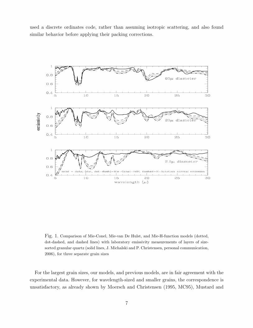
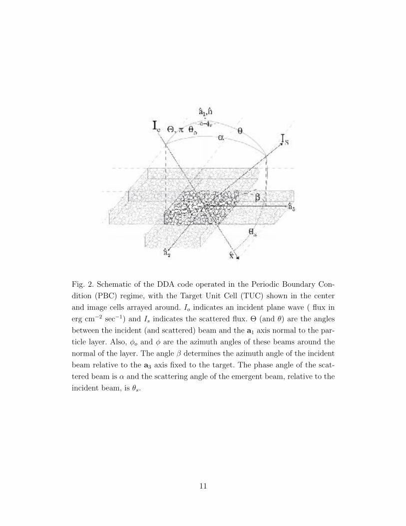
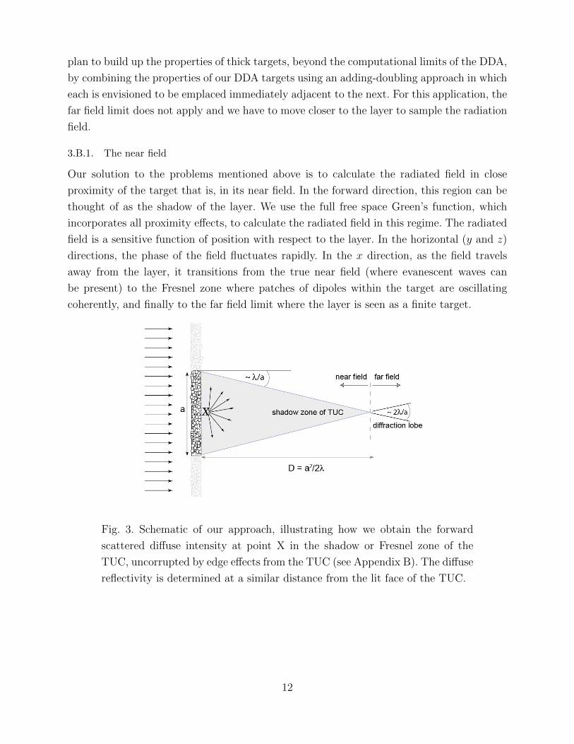
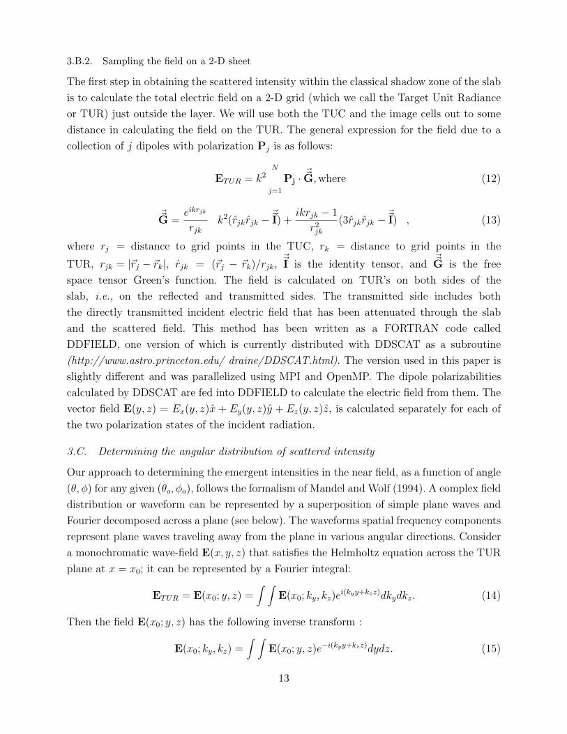
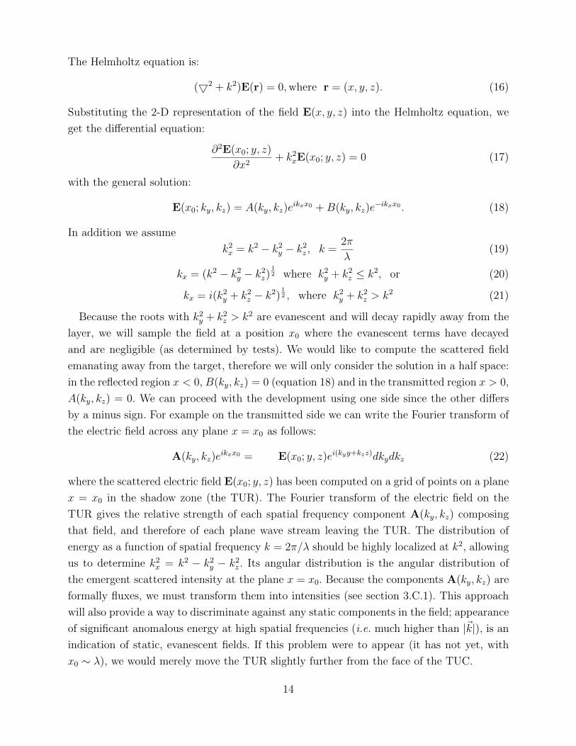
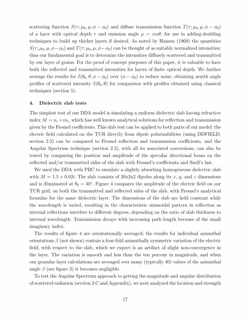
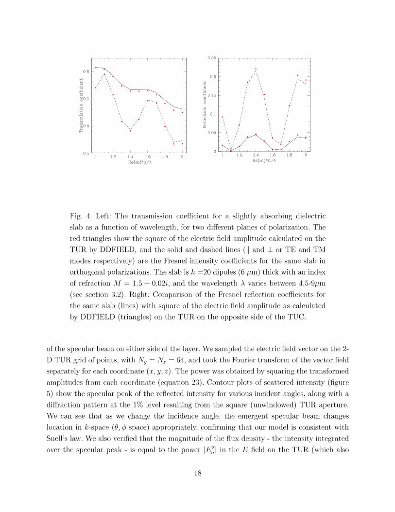
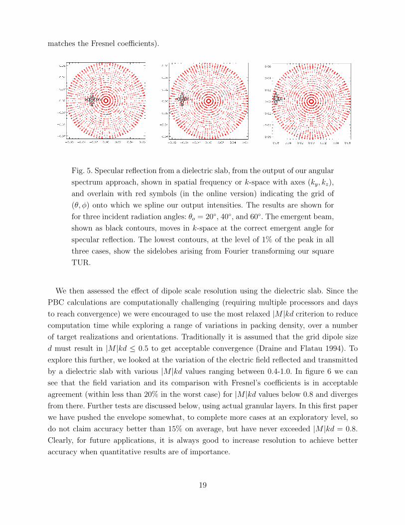
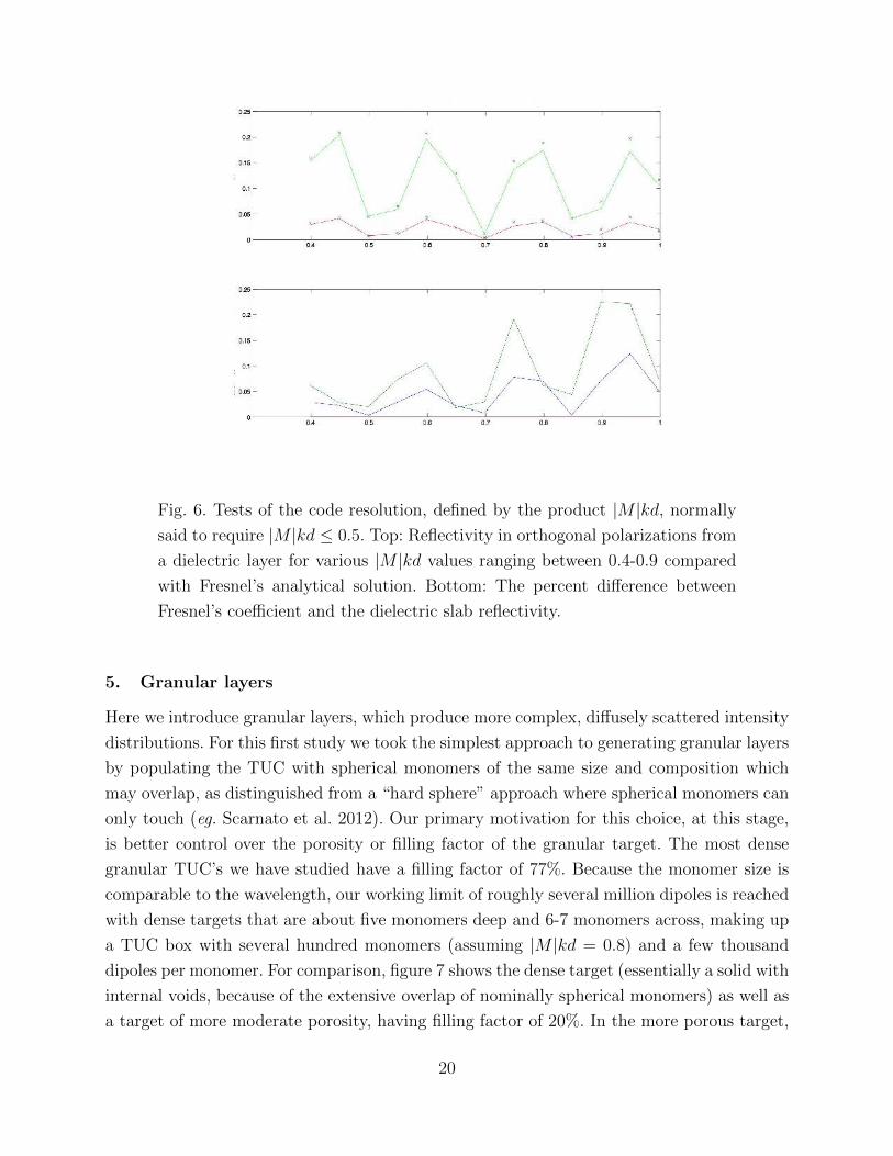
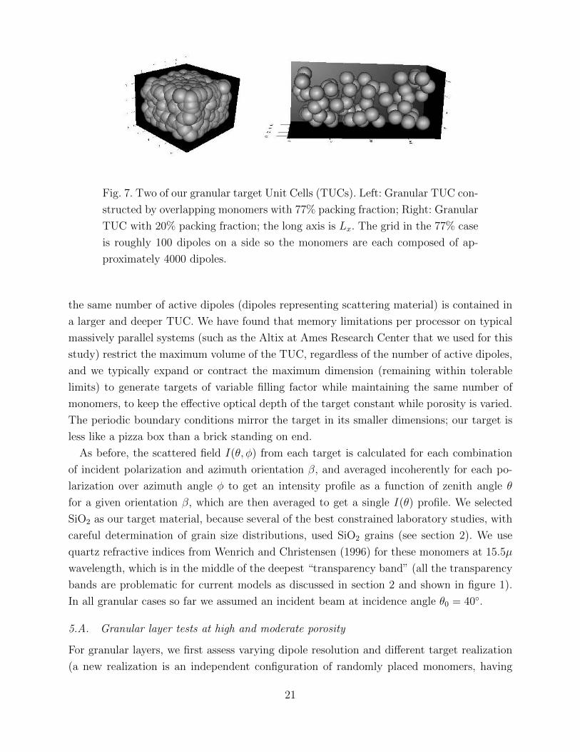
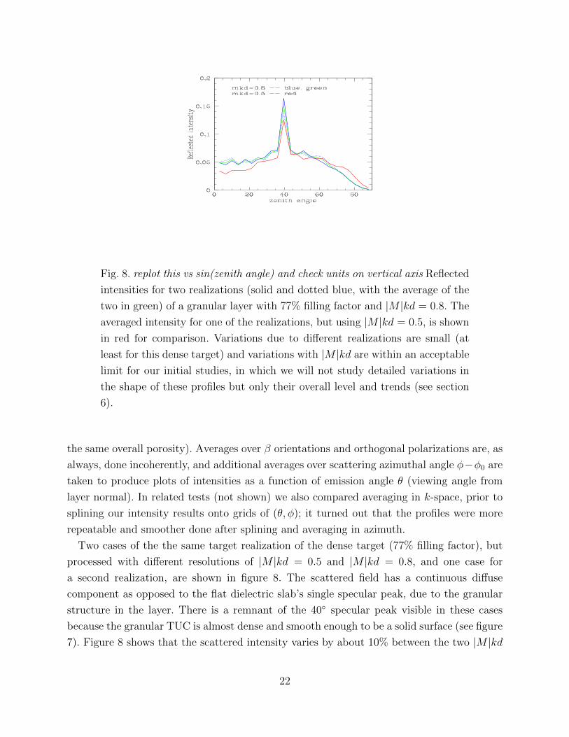
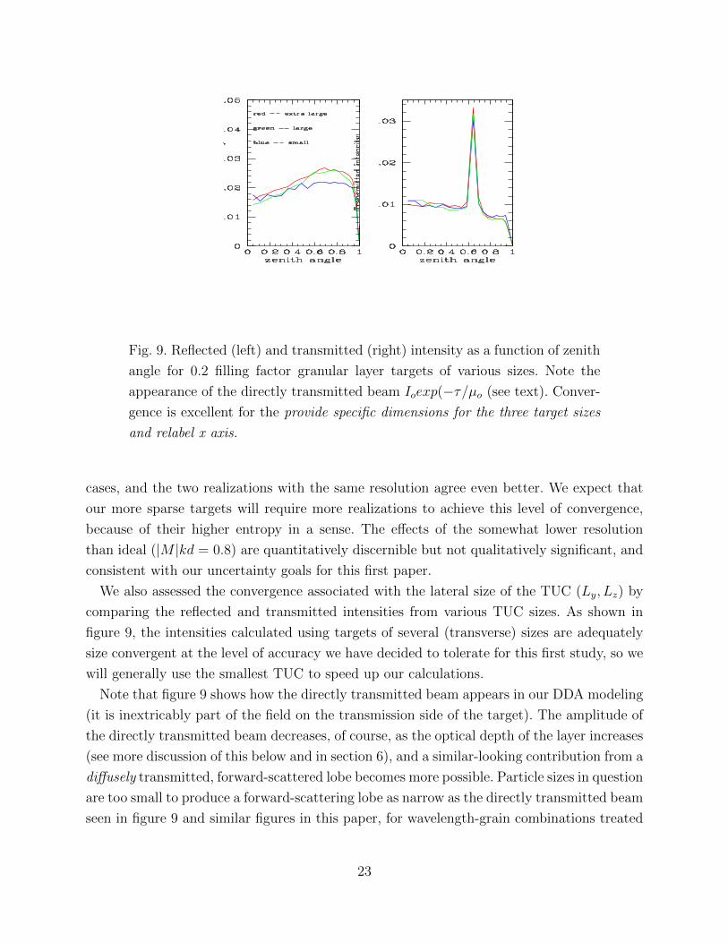
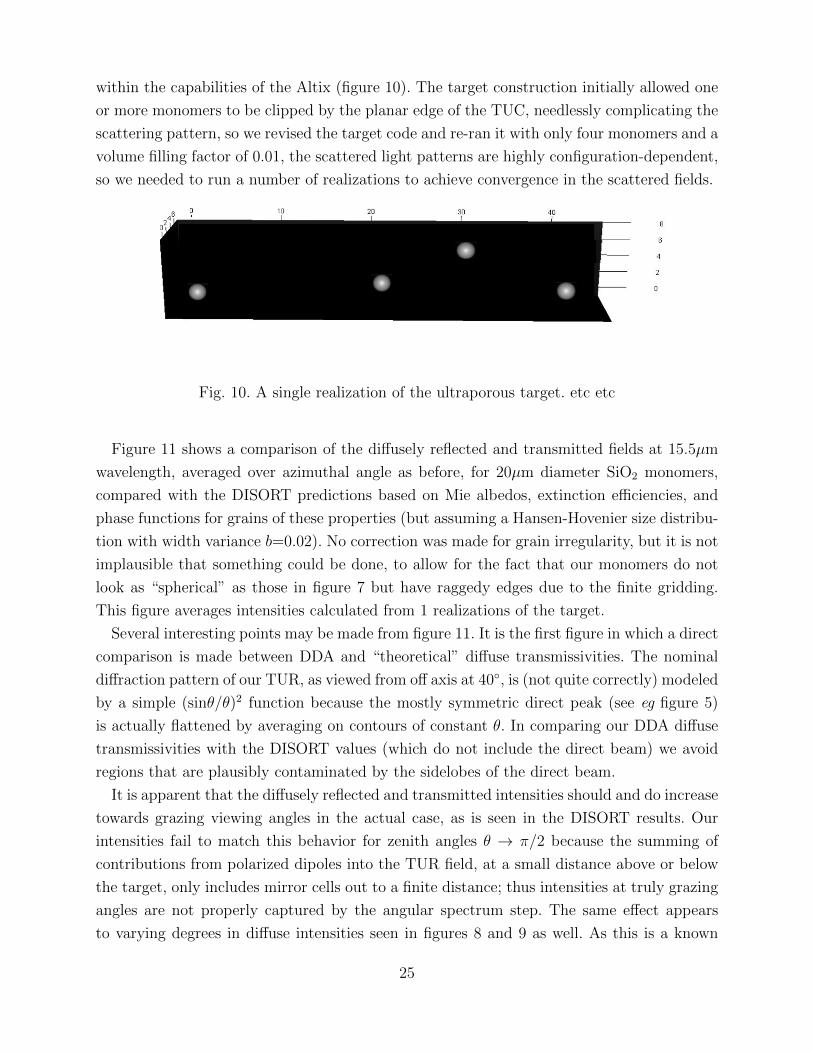
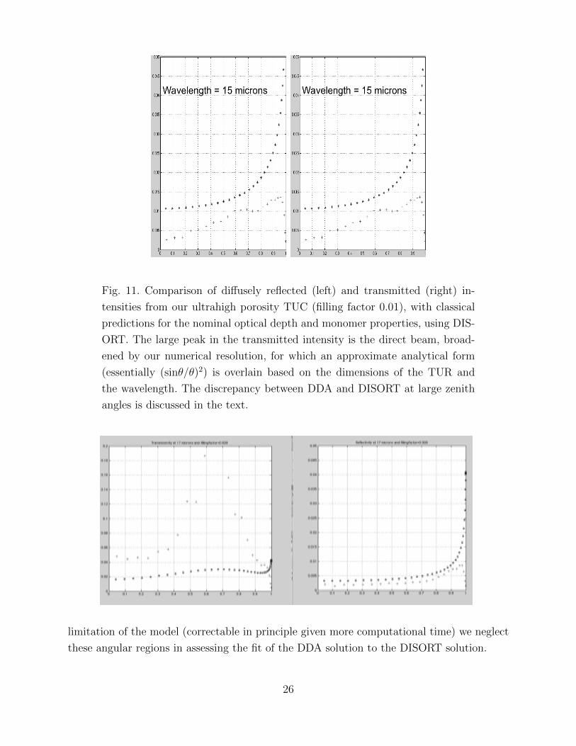
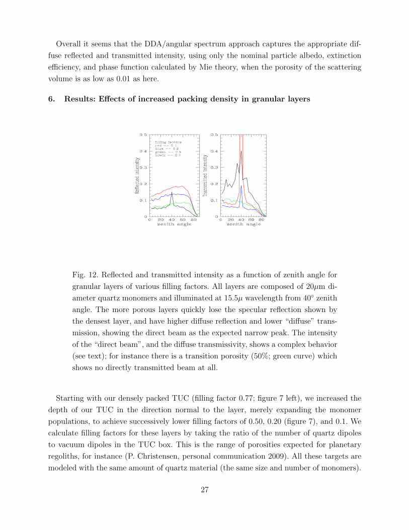
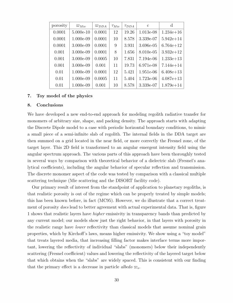
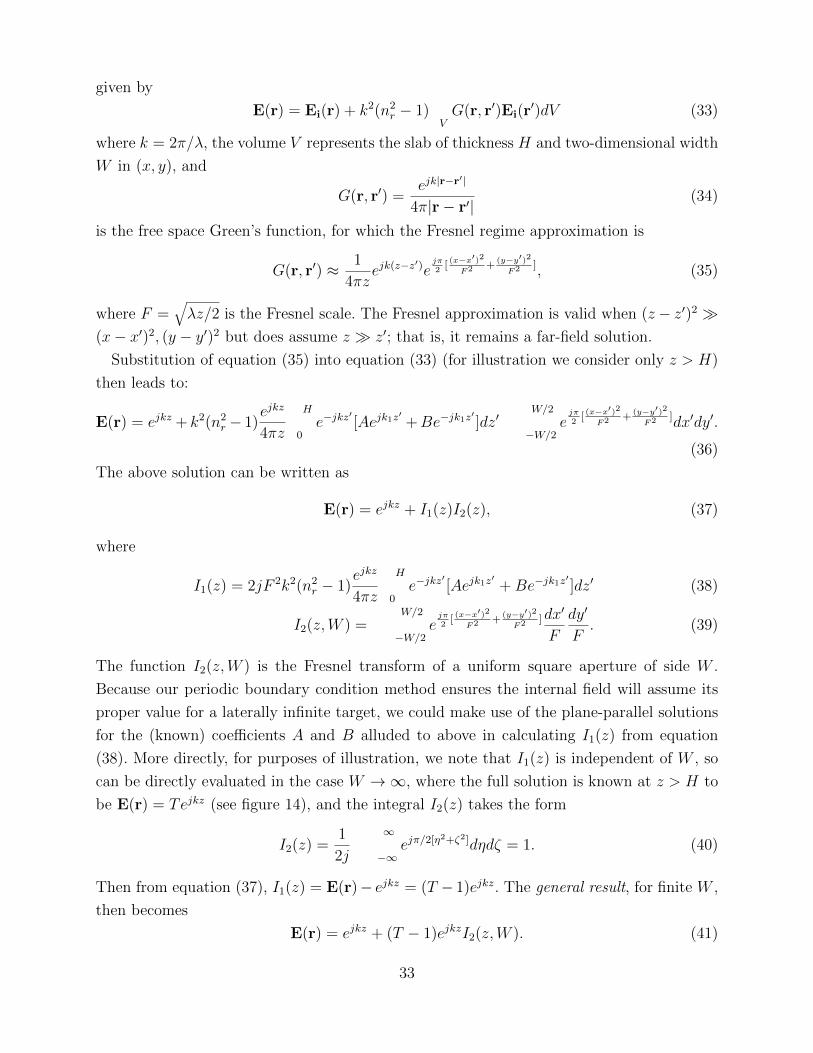
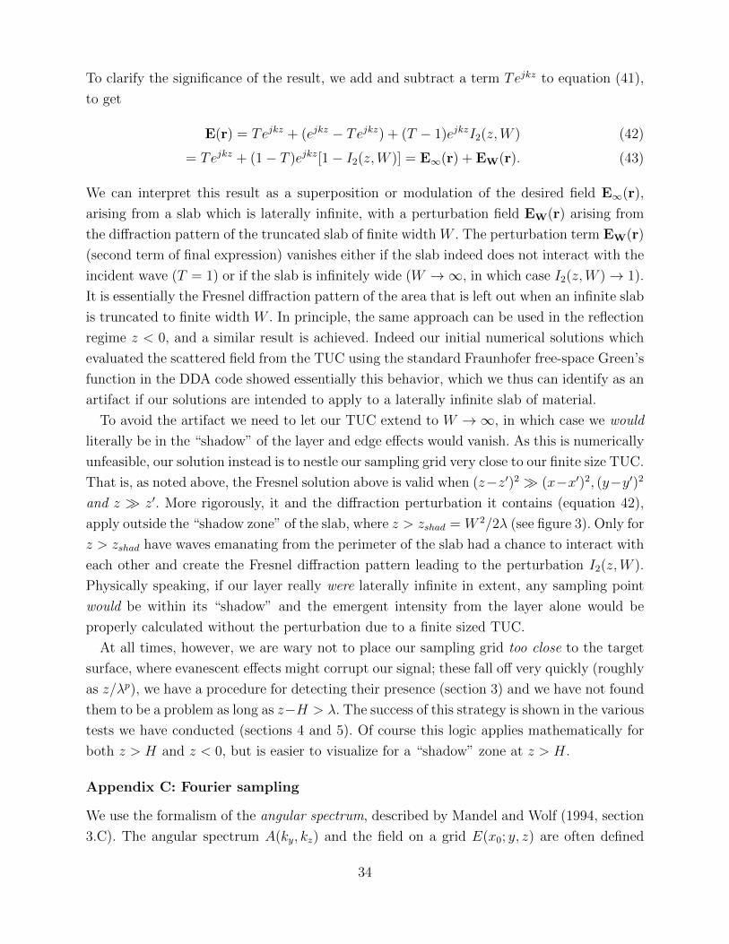
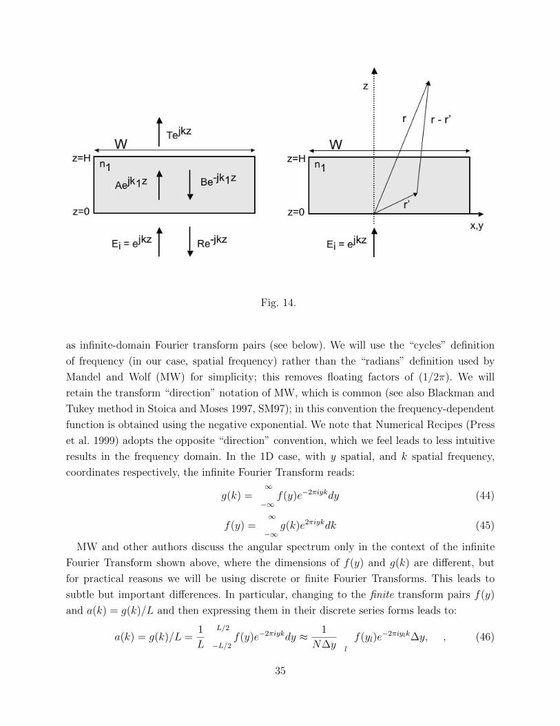
Recommended