Distributed Local Search Based on a Parallel
Neighborhood Exploration for the Rooted
Distance-Constrained Minimum
Spanning-Tree Problem
Master Thesis
Presented in partial fulfillment to obtain the Title of
Magister in Informatics and Telecommunications
by
Cesar David Loaiza Quintana
Advisor: Gabriel Tamura, PhD
Co-Advisors: Luis Quesada, PhD; Andres Aristizabal, PhD
Department of Information and Communication Technologies
Faculty of Engineering
July, 2019
Contents
List of Tables iii
List of Figures iv
1 Introduction 2
1.1 Context and Motivation . . . . . . . . . . . . . . . . . . . . . . . . . . . . . . . . . . 2
1.2 Problem Description . . . . . . . . . . . . . . . . . . . . . . . . . . . . . . . . . . . . 4
1.3 Challenges . . . . . . . . . . . . . . . . . . . . . . . . . . . . . . . . . . . . . . . . . . 4
1.4 Research Objectives . . . . . . . . . . . . . . . . . . . . . . . . . . . . . . . . . . . . 5
1.4.1 General . . . . . . . . . . . . . . . . . . . . . . . . . . . . . . . . . . . . . . . 5
1.4.2 Specific . . . . . . . . . . . . . . . . . . . . . . . . . . . . . . . . . . . . . . . 5
1.5 Methodology . . . . . . . . . . . . . . . . . . . . . . . . . . . . . . . . . . . . . . . . 5
1.6 Thesis Organization . . . . . . . . . . . . . . . . . . . . . . . . . . . . . . . . . . . . 6
1.7 Contribution Summary . . . . . . . . . . . . . . . . . . . . . . . . . . . . . . . . . . . 6
2 Theoretical Background and State of the Art 7
2.1 Minimum Spanning Trees . . . . . . . . . . . . . . . . . . . . . . . . . . . . . . . . . 7
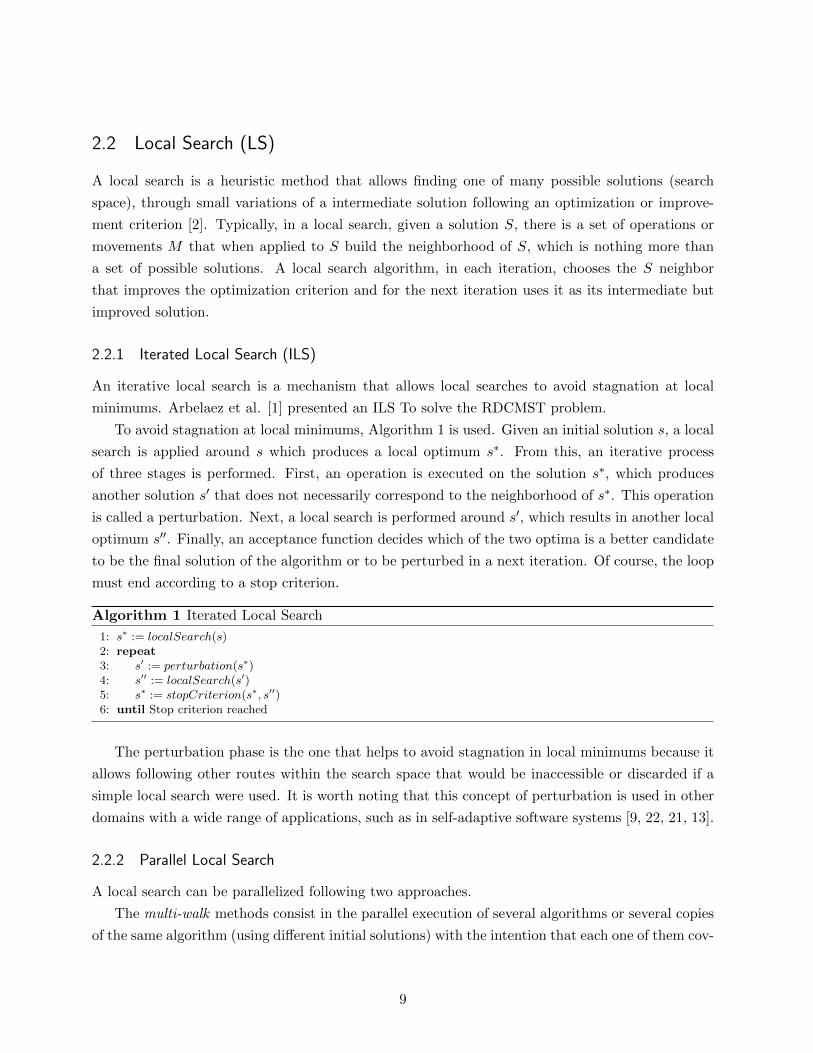
2.2 Local Search (LS) . . . . . . . . . . . . . . . . . . . . . . . . . . . . . . . . . . . . . . 9
2.2.1 Iterated Local Search (ILS) . . . . . . . . . . . . . . . . . . . . . . . . . . . . 9
2.2.2 Parallel Local Search . . . . . . . . . . . . . . . . . . . . . . . . . . . . . . . . 9
2.3 Hadoop . . . . . . . . . . . . . . . . . . . . . . . . . . . . . . . . . . . . . . . . . . . 10
2.3.1 The Hadoop Distributed File System (HDFS) . . . . . . . . . . . . . . . . . . 10
2.3.2 Yet Another Resouce Negotiator (YARN) . . . . . . . . . . . . . . . . . . . . 10
2.3.3 Hadoop MapReduce . . . . . . . . . . . . . . . . . . . . . . . . . . . . . . . . 11
2.4 Giraph . . . . . . . . . . . . . . . . . . . . . . . . . . . . . . . . . . . . . . . . . . . . 11
2.4.1 Data Model . . . . . . . . . . . . . . . . . . . . . . . . . . . . . . . . . . . . . 11
2.4.2 Bulk Synchronous Parallel Model . . . . . . . . . . . . . . . . . . . . . . . . . 12
2.4.3 Basic Computation . . . . . . . . . . . . . . . . . . . . . . . . . . . . . . . . . 13
2.4.4 Combiners . . . . . . . . . . . . . . . . . . . . . . . . . . . . . . . . . . . . . . 15
i

2.4.5 Giraph Architecture . . . . . . . . . . . . . . . . . . . . . . . . . . . . . . . . 16
2.4.6 Master Computation and Shared State . . . . . . . . . . . . . . . . . . . . . . 17
3 Understanding the Giraph Computation Model 21
3.1 A simple problem . . . . . . . . . . . . . . . . . . . . . . . . . . . . . . . . . . . . . . 21
3.2 Using the advanced Giraph’s features . . . . . . . . . . . . . . . . . . . . . . . . . . . 22
3.2.1 Data model . . . . . . . . . . . . . . . . . . . . . . . . . . . . . . . . . . . . . 23
3.2.2 Master compute . . . . . . . . . . . . . . . . . . . . . . . . . . . . . . . . . . 23
3.2.3 Basic computation . . . . . . . . . . . . . . . . . . . . . . . . . . . . . . . . . 23
3.2.4 Aggregator . . . . . . . . . . . . . . . . . . . . . . . . . . . . . . . . . . . . . 26
4 The Global Design Strategy Exploiting Giraph 27
4.1 An Iterated Local Search to solve RDCMST . . . . . . . . . . . . . . . . . . . . . . . 27
4.1.1 The problem . . . . . . . . . . . . . . . . . . . . . . . . . . . . . . . . . . . . 27
4.1.2 The sequential algorithm . . . . . . . . . . . . . . . . . . . . . . . . . . . . . 27
4.1.3 Towards a parallel solution . . . . . . . . . . . . . . . . . . . . . . . . . . . . 29
4.2 Using Giraph to Solve RDCMST: A Complete Solution . . . . . . . . . . . . . . . . 31
4.2.1 Data model . . . . . . . . . . . . . . . . . . . . . . . . . . . . . . . . . . . . . 31
4.2.2 Master compute . . . . . . . . . . . . . . . . . . . . . . . . . . . . . . . . . . 33
4.2.3 Delete operation . . . . . . . . . . . . . . . . . . . . . . . . . . . . . . . . . . 34
4.2.4 Insert operation . . . . . . . . . . . . . . . . . . . . . . . . . . . . . . . . . . 44
5 Evaluation 53
5.1 The Computational Infrastructure . . . . . . . . . . . . . . . . . . . . . . . . . . . . 53
5.2 Dataset . . . . . . . . . . . . . . . . . . . . . . . . . . . . . . . . . . . . . . . . . . . 53
5.3 Distance Constraint λ . . . . . . . . . . . . . . . . . . . . . . . . . . . . . . . . . . . 55
5.4 Pilot Experiments Phase . . . . . . . . . . . . . . . . . . . . . . . . . . . . . . . . . . 55
5.5 Small instances . . . . . . . . . . . . . . . . . . . . . . . . . . . . . . . . . . . . . . . 56
5.6 Big Instances . . . . . . . . . . . . . . . . . . . . . . . . . . . . . . . . . . . . . . . . 57
5.7 Results Analysis . . . . . . . . . . . . . . . . . . . . . . . . . . . . . . . . . . . . . . 60
5.7.1 The use of Apache Giraph . . . . . . . . . . . . . . . . . . . . . . . . . . . . . 60
5.7.2 An Implementation for Big Data . . . . . . . . . . . . . . . . . . . . . . . . . 61
5.7.3 Final remarks . . . . . . . . . . . . . . . . . . . . . . . . . . . . . . . . . . . . 61
6 Conclusions and Future Work 63
A Movement illustration 65
Bibliography 80
ii

List of Tables
5.1 Datasets’ size . . . . . . . . . . . . . . . . . . . . . . . . . . . . . . . . . . . . . . . . 56
5.2 Execution during 30 minutes on random small instances . . . . . . . . . . . . . . . . 57
5.3 Experiments’ Execution Time in minutes . . . . . . . . . . . . . . . . . . . . . . . . 57
5.4 Results of the experiments in terms of cost . . . . . . . . . . . . . . . . . . . . . . . 58
5.5 Results using different initial solutions . . . . . . . . . . . . . . . . . . . . . . . . . . 60
iii
List of Figures
1.1 An example of a Long-Reach Passive Optical Network. Adapted from [1] . . . . . . . 3
2.1 Bulk Synchronous Parallel Model . . . . . . . . . . . . . . . . . . . . . . . . . . . . . 13
2.2 Computation of a vertex that propagates the largest value received . . . . . . . . . . 14
2.3 Messages reduced by a Max combiner . . . . . . . . . . . . . . . . . . . . . . . . . . 16
2.4 Giraph Architecture . . . . . . . . . . . . . . . . . . . . . . . . . . . . . . . . . . . . 18
2.5 The master node is a centralized point of computation. Its compute() method is
executed once before each superstep. Aggregator values are passed from and to the
vertices . . . . . . . . . . . . . . . . . . . . . . . . . . . . . . . . . . . . . . . . . . . 19
3.1 A simple problem’s solution . . . . . . . . . . . . . . . . . . . . . . . . . . . . . . . . 21
3.2 Supersteps to find the average path length to farthest leaf . . . . . . . . . . . . . . . 25
4.1 Delete Operation . . . . . . . . . . . . . . . . . . . . . . . . . . . . . . . . . . . . . . 30
4.2 Insert operation’s scenarios . . . . . . . . . . . . . . . . . . . . . . . . . . . . . . . . 30
4.3 Partial solution for RDCMST problem . . . . . . . . . . . . . . . . . . . . . . . . . . 32
4.4 Feasible Delete Strategy . . . . . . . . . . . . . . . . . . . . . . . . . . . . . . . . . . 34
4.5 Update of the f attributes after vertex deletion . . . . . . . . . . . . . . . . . . . . . 39
4.6 Update of the b attributes after vertex deletion . . . . . . . . . . . . . . . . . . . . . 41
4.7 Scenarios for the new farthest leaf . . . . . . . . . . . . . . . . . . . . . . . . . . . . 42
4.8 Example of the two type of location for vertex n3 . . . . . . . . . . . . . . . . . . . . 46
5.1 Deployment diagram . . . . . . . . . . . . . . . . . . . . . . . . . . . . . . . . . . . . 54
5.2 Number of threads per working performing 10000 movements . . . . . . . . . . . . . 56
5.3 Locations evaluated per minute . . . . . . . . . . . . . . . . . . . . . . . . . . . . . . 59
A.1 Movement Illustration . . . . . . . . . . . . . . . . . . . . . . . . . . . . . . . . . . . 67
A.1 Movement Illustration . . . . . . . . . . . . . . . . . . . . . . . . . . . . . . . . . . . 68
A.1 Movement Illustration . . . . . . . . . . . . . . . . . . . . . . . . . . . . . . . . . . . 69
A.1 Movement Illustration . . . . . . . . . . . . . . . . . . . . . . . . . . . . . . . . . . . 70
iv
A.1 Movement Illustration . . . . . . . . . . . . . . . . . . . . . . . . . . . . . . . . . . . 71
A.1 Movement Illustration . . . . . . . . . . . . . . . . . . . . . . . . . . . . . . . . . . . 72
A.1 Movement Illustration . . . . . . . . . . . . . . . . . . . . . . . . . . . . . . . . . . . 73
A.1 Movement Illustration . . . . . . . . . . . . . . . . . . . . . . . . . . . . . . . . . . . 74
A.1 Movement Illustration . . . . . . . . . . . . . . . . . . . . . . . . . . . . . . . . . . . 75
A.1 Movement Illustration . . . . . . . . . . . . . . . . . . . . . . . . . . . . . . . . . . . 76
A.1 Movement Illustration . . . . . . . . . . . . . . . . . . . . . . . . . . . . . . . . . . . 77
A.1 Movement Illustration . . . . . . . . . . . . . . . . . . . . . . . . . . . . . . . . . . . 78
A.1 Movement Illustration . . . . . . . . . . . . . . . . . . . . . . . . . . . . . . . . . . . 79
v
Abstract
The Rooted Distance-Constrained Minimum Spanning-Tree Problem (RDCMST) is an optimiza-
tion problem known to be NP-hard whose solution can be applied to the design of telecommuni-
cations networks, among others. Previous research to solve the RDCMST problem have proposed
solutions ranging from exact algorithms, such as classic linear programming models, to heuristic
methods that include the use of local searches. To the best of our knowledge, the state of the
art of this problem has at least two critical shortcomings. On the one hand, there are no parallel
approaches that have been designed to take advantage of several processing units. On the other
hand, existing approaches are limited to instances of the problem of a few thousand vertices.
This master’s thesis focuses on the construction of a distributed strategy to solve the RDCMST
problem from a local search, which performs a parallel exploration of the neighborhood. Moreover,
this strategy was implemented in distributed software that allows dealing with instances of the
problem of tens of thousands of vertices. In order to achieve the above, we faced challenges mainly
associated with the performance of the solution, and therefore, with the appropriate use of the
available computing resources. Most of these challenges were overcome by adopting the Apache
Giraph graph processing framework. Therefore, this work also allowed us to study how suitable
Giraph is to solve similar problems.
Besides the strategy to solve RDCMST and its implementation in a distributed environment,
the contribution of this work includes a series of algorithms designed to be executed in parallel
using multiple processing nodes, which solve common issues in the design of graph problem’s
solutions. Finally, we made an experimental evaluation of the strategy, which showed that it is
capable of handling instances of tens of thousands of vertices in a reasonable amount of time.
Furthermore, the evaluation indicates that the implemented software may work better with even
larger instances and that it may perform better under certain conditions of the initial sub-optimal
solution in the local search.
Resumen
El Rooted Distance-Constrained Minimum Spanning-Tree Problem (Problema de Arbol de Re-
cubrimiento Mınimo Acotado por Distancia con Raız Fija, RDCMST por sus iniciales en ingles)
es un problema de optimizacion conocido por ser NP-hard cuya solucion se puede aplicar al diseno
de redes de telecomunicaciones, entre otros. Investigaciones previas para resolver el problema RD-
CMST han propuesto soluciones que van desde algoritmos exactos, como los modelos clasicos de
programacion lineal, hasta metodos heurısticos que incluyen el uso de busquedas locales. Por lo
que sabemos, el estado del arte de este problema tiene al menos dos carencias importantes. Por un
lado, no existen aproximaciones paralelas que hayan sido disenadas para aprovechar varias unidades
de procesamiento. Por el otro lado, las aproximaciones existentes estan limitadas a instancias del
problema de unos pocos miles de vertices.
Esta tesis de maestrıa se centra en la construccion de una estrategia distribuida para resolver
el problema RDCMST a partir de una busqueda local, la cual realiza una exploracion paralela del
vecindario. Mas aun, esta estrategia fue implementada en un software distribuido que permite lidiar
con instancias del problema de cientos de miles de vertices. Para lograr lo anterior, se afrontaron
retos asociados principalmente al desempeno de la solucion, y por tanto, al uso adecuado de los
recursos computacionales disponibles. La mayorıa de dichos retos fueron superados mediante la
adopcion del framework para procesamiento de grafos Apache Giraph. Por lo tanto, este trabajo
tambien permitio estudiar que tan adecuado es el uso de Giraph para resolver problemas similares.
Ademas de la estrategia para resolver RDCMST y su implementacion en un ambiente dis-
tribuido, la contribucion de este trabajo incluye una serie de algoritmos disenados para ser ejecu-
tados en paralelo en distintos nodos de procesamiento, los cuales resuelven problemas comunes en
el diseno de soluciones a problemas de grafos. Finalmente, se realizo una evaluacion experimental
de la estrategia que mostro que esta es capaz de manejar instancias de decenas de miles de vertices
en un tiempo razonable. Ademas, la evaluacion da indicios de que el software implementado puede
funcionar mejor con instancias incluso mas grandes y que puede tener un mejor desempeno bajo
ciertas condiciones de la solucion sub-optima inicial en la busqueda local.
1

Dedication
To my family, who always support and love me.
1
Acknowledgments
I would like to express my gratitude to my advisors Dr. Gabriel Tamura and Dr. Andres
Aristizabal of the Department of Information and Telecommunication Technologies, School of En-
gineering at Icesi University, and Dr. Luis Quesada of the Insight Centre for Data Analytics,
University College Cork. Without their ideas, work, and guidance, this thesis would not have been
possible. I hope to keep learning from them.
I would like to thank the professors of the School of Engineering at Icesi University who, during
my master, taught me and helped me to find this research path finally.
Lastly, I am grateful to the Center of Excellence and appropriation in Big Data and Data
Analytics (Alianza CAOBA) for granting me a full-tuition scholarship for this master.
1
Chapter 1
Introduction
1.1 Context and Motivation
Optimization problems can be formulated in terms of finding and choosing a solution that maximizes
a set of criteria, among a set of candidate solutions. A local search is a heuristic method that allows
complex problems of optimization to be addressed, finding solutions that, although they are not
the optimum, offer a good approximation to it. This is why the applications of local searches cover
fields of knowledge as general as computer science, mathematics, engineering or bioinformatics.
In many cases, in the optimization problems, the set of possible solutions is limited by a set
of restrictions. In the design of a telecommunications network for a geographical region, for ex-
ample, the goal is to minimize the cost of its implementation, and there are many cases in which
this implementation is restricted by a distance constraint originated by the delay or signal loss.
Moreover, there are problem sets that require a path between a particular vertex of the network
and all the remaining vertices, such that those paths do not exceed a limit in their length, and the
amount of used cable is minimized. These problems are instances of an NP-hard problem known as
the Rooted Distance-Constrained Minimum Spanning Tree Problem (RDCMST). In the RDCMST
problem, given a weighted graph and a root vertex, we must find a Minimum Spanning Tree in
which the shortest path from any vertex to the root does not exceed a certain threshold.
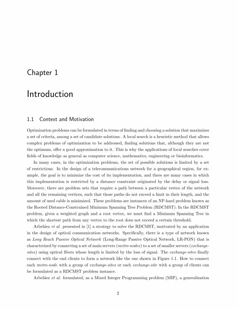
Arbelaez et al. presented in [1] a strategy to solve the RDCMST, motivated by an application
in the design of optical communication networks. Specifically, there is a type of network known
as Long Reach Passive Optical Network (Long-Range Passive Optical Network, LR-PON) that is
characterized by connecting a set of main servers (metro-nodes) to a set of smaller servers (exchange-
sites) using optical fibers whose length is limited by the loss of signal. The exchange-sites finally
connect with the end clients to form a network like the one shown in Figure 1.1. How to connect
each metro-node with a group of exchange-sites or each exchange-site with a group of clients can
be formulated as a RDCMST problem instance.
Arbelaez et al. formulated, as a Mixed Integer Programming problem (MIP), a generalization
2

Figure 1.1: An example of a Long-Reach Passive Optical Network. Adapted from [1]
of RDCMST called Edge-Disjoint Rooted Distance-Constrained Minimum Spanning-Tree Prob-
lem (ERDCMST), which in a nutshell is a set of overlapped RDCMST instances with an edge-
disjointness restriction. Arbelaez et al. also proposed an Iterated Constraint-based Local Search
(ICBLS) that is able to solve both ERDCMST and RDCMST. Furthermore, in the same paper,
they presented a parallel extension of their algorithm only for ERDCMST, which basically can solve
many RDCMST instances in parallel, but with stringent limitations on the graph size. However,
to the best of our knowledge there are no known approaches to solve the RDCMST problem in
parallel nor in distributed way.
In the ICBLS proposed by Arbelaez et al., the search space is made up of all possible Spanning
Trees that satisfy the problem constraints. Given a suboptimal solution S, an m operation is
applied iteratively over S to build the neighborhood of S in the search space. In each iteration of
the local search, the algorithm chooses the neighboring solution of S that minimizes the sum of
the weights of all the edges of the tree. This operation m makes changes in the structure of the
tree that makes up the tree that represents the approximate solution. Then, the exploration of
the neighborhood in the algorithm consists of applying the operator m to the solution S as many
times as necessary to generate a good amount of possible solutions derived from S that meet the
restrictions of the problem. After this, we must compute the cost of all possible solutions and
choose the best option.
The Simplex method [14] is an algorithm that solves linear programming problems through
an exhaustive search, guaranteeing an optimal solution. The ICBLS proposed by Arbelaez et al.
finds acceptable solutions in a considerably shorter time than the simplex method for the MIP
3
formulation, which even overflows the memory for relative small entries. Still, the ICBLS has
serious limitations on the size of the input problem.
1.2 Problem Description
As we mentioned in Section 1.1, Arbelaez et al. proposed a sequential algorithm based on a
local search to solve the RDCMST problem. However, to the best of our knowledge, no known
distributed nor parallel strategy has been presented to solve the problem. An approach, that
has been previously studied in the context of local searches, is conducting the exploration of the
neighborhood in parallel, which must be designed using distributed algorithms in order to overcome
limitations on the size of the input problem.
Problem Statement
The problem object of the present work is stated as follows: How to solve the RDCMST problem
through a parallel neighborhood exploration strategy overcoming the limitations on the input size?
1.3 Challenges
To solve the stated problem, it will be necessary to address important challenges. These challenges,
listed below, focus on the most important aspects to solve in the problem:
• In order to maximize the parallelization of neighborhood exploration, we have to define a
proper task granularity. What should be an adequate task granularity that allows us to
obtain a higher level of parallelism?
• How to design a distribution strategy that allows maximizing the use of computational
resources and minimizing communication between distributed tasks? Which graph-based
paradigm of distributed computing is more convenient for the design and implementation of
the strategy?
• How can we encode the whole local search algorithm for RDCMST in the limited program-
ming models that are supported by the state-of-the-art graph-based distributed computing
frameworks?
• How to evaluate the solution in a way that is comparable to the approaches published in the
state of the art?
4

1.4 Research Objectives
1.4.1 General
Build a distributed local search with a parallel neighborhood exploration strategy based on a
distributed software architecture to solve the RDCMST problem, balancing load distribution, as
far as possible, uniformly among the available processors enabled for processing large input graphs.
1.4.2 Specific
To fulfill the general objective, we identify the following specific objectives:
1. Find an adequate task’s granularity that allows a load distribution as uniform as possible to
execute the distributed local search.
2. Design a distributed program that implements the solution strategy in a way that exploits
the paradigms of graph distributed computing.
3. Evaluate, experimentally, the correctness and performance of the solution and compare it
with published state-of-the-art solutions.
1.5 Methodology
To fulfill the stated goals, we used the mixed research method [4], combining quantitative methods
and qualitative methods.
It is necessary to collect and analyze qualitative data in three phases.
1. The literature review on solutions for similar problems.
2. The literature review on the paradigms and techniques of distributed computing and pro-
gramming.
3. The analysis of the nature of the problem that, in conjunction with its size and the compu-
tational resources available, give rise to the design of the strategy.
The collection and analysis of quantitative data are necessary to experimentally evaluate the
proposed solution strategy. This evaluation will be carried out based on the performance obtained
by the execution of the solution in different scenarios that involve the computational infrastructure
or the input parameters. For this, it will be necessary to design multiple experiments applied to
instances of the RDCMST problem. These instances are expected to come from real deployments
of a passive optical network in Spain, as well as from artificially generated graphs.
5

1.6 Thesis Organization
The remaining chapters of this thesis are organized as follows. Chapter 2 presents the background
and state of the art related to the problem we tackle in this thesis and the toolset that we use to
solve it. Chapter 3 extends the explanation of Giraph’s computing model by analyzing solutions
for simpler problems. Chapter 4 introduces the sequential Local Search strategy on which we
based our approach. This local search strategy motivates some of the ideas that led us to work on
this project. Moreover, it presents our distributed strategy to solve the problem using the Giraph
framework, describing how we adapted every logic unit of the sequential algorithm to the Giraph’s
programming model. Chapter 5 details the evaluation of the strategy using real and artificial
instances, which revealed the pros and cons of our implementation. Finally, Chapter 6 concludes
this thesis and proposes future work.
1.7 Contribution Summary
The main contributions of this thesis are:
1. The design of a distributed strategy that performs a parallel exploration of the neighborhood
to solve the RDCMST problem.
2. The implementation of the strategy proposed in a scalable and executable distributed software
that works for large graphs, which is based on a flexible granularity that allows an automatic
uniform balance distribution regardless the number of processing nodes.
3. A series of algorithms, which were designed to be executed in a distributed enviroment, that
solve common issues in the design of graph problem’s solutions.
4. An experimental evaluation of the software implemented with a real case.
6
Chapter 2
Theoretical Background and State of the Art
This chapter gives the background and the state of the art related to the problem we tackle in this
thesis and the toolset that we use to solve it, from abstract mathematical strategies to software
frameworks.
2.1 Minimum Spanning Trees
The minimum spanning tree [6] of a weighted non-directed graph is the tree that connects all
the vertices of the graph, in such a way that the sum of the weights of its edges is minimized.
Finding that tree is a problem widely studied in computer science, which since 1930 has been
solved in polynomial time using greedy algorithms, and whose solution today can be found in
linear or almost linear time. Additionally, parallel/distributed algorithms that find a solution to
the problem faster than optimized sequential algorithms have been proposed.
Several problems have arisen from the Minimum Spanning Tree problem, some of which are
computationally much more complex than the original and require radically different strategies to
be solved.
Rooted Distance-Constrained Minimum Spanning-Tree Problem (RDCMST)
The Rooted Distance-Constrained Minimum Spanning-Tree Problem can be defined as follows:
given a weighted graph G = (V,E) with a root node r ∈ V , find a minimum spanning tree such
that the distance of a path in the tree between any node v ∈ V and the root r does not exceed a
constant λ threshold.
The RDCMST is a famous problem in the design network field known to be NP-Hard [15][7].
The complexity of the problem could be easily understood if it is seen as a generalization of the
hop-constrained minimum spanning tree problem, which is shown to be NP-Hard in [5].
Some exact algorithms that produce the optimal solution to the problem have been proposed.
J Oh, I Pyo, M Pedram [15] proposed an algorithm based on iterative negative sum exchanges
7
and L Gouveia, A Paias and D Sharma [7] presented two approaches. The first one following a
column generation scheme and the second one through a Lagrangian relaxation combined with
a subgradient optimization procedure. Furthermore, classic linear programming approaches have
been modeled and used in [1] and [7]. These methods can handle only graphs of a few hundreds of
nodes.
In order to solve larger instances of the problem, several heuristic approaches have been intro-
duced including a local iterative search. Some of these heuristic methods were designed using the
ideas of the most classic greedy algorithms to solve MST: the Prim’s algorithm and the Kruskal’s
algorithm.
A Prim’s-based heuristic was presented by Salama et al. in [20]. Starting from the root node,
the algorithm builds the tree by iteratively adding the node that can be reached in the cheapest
way without violating the distance constraint. When no more nodes can be added, the distance
constraint is tried to be relaxed by changing some of the edges of the nodes that have been already
added to the tree. Then, if all nodes have been added, a second phase using the edge-exchange
process is used to reduce the final cost of the solution.
J Oh, I Pyo and M Pedram [15] presented the Bounded KRUSkal (BKRUS) algorithm, which,
as in its classic version, starts with a completed disconnected graph and in each step picks the
best possible edge (the one with the minimum weight) that joins two graph’s components until the
graph is fully connected. However, in this version in every step, the algorithm is very careful that
there will not be a chance to violate the distance constraint in the resulting tree. Additionally, M
Ruthmair and GR Raidl [16] presented a very similar Kruskal-based approach. These Kruskal-based
approaches are prone to outperform Prim-based ones in Euclidean instances because it performs
more global searches, which can avoid the distance wasting that can happen in the surrounding
root’s neighborhood of a prim-based solution.
Some other soft computing approaches have been proposed. Berlakovich M, Ruthmair M and
Raidl GR [3] presented a Local Search based on a ranking score, which arranges the edges using
their potential convenience according to the distance constraint. This approach incorporates the
distance constraint to the heuristic, unlike the classic ones that ignore it while it is not violated.
Ruthmair, M. and Raidl, G.R. [17] proposed two methods. The first is based on the principles
of Ant Colony Optimization (ACO) which in turn conducts neighborhood explorations on two
different structures. The second is a Variable Neighborhood Search (VNS) that uses the same
neighborhood structures but introduces edge exchanges to disturb the solutions. In most cases, the
ACO was better than the VNS. An additional and very similar method to the previous one was
presented in [18], this time using a genetic algorithm to conduct the neighborhood exploration. All
of these methods have been validated in graphs of up to 1000 vertices.
8
2.2 Local Search (LS)
A local search is a heuristic method that allows finding one of many possible solutions (search
space), through small variations of a intermediate solution following an optimization or improve-
ment criterion [2]. Typically, in a local search, given a solution S, there is a set of operations or
movements M that when applied to S build the neighborhood of S, which is nothing more than
a set of possible solutions. A local search algorithm, in each iteration, chooses the S neighbor
that improves the optimization criterion and for the next iteration uses it as its intermediate but
improved solution.
2.2.1 Iterated Local Search (ILS)
An iterative local search is a mechanism that allows local searches to avoid stagnation at local
minimums. Arbelaez et al. [1] presented an ILS To solve the RDCMST problem.
To avoid stagnation at local minimums, Algorithm 1 is used. Given an initial solution s, a local
search is applied around s which produces a local optimum s∗. From this, an iterative process
of three stages is performed. First, an operation is executed on the solution s∗, which produces
another solution s′ that does not necessarily correspond to the neighborhood of s∗. This operation
is called a perturbation. Next, a local search is performed around s′, which results in another local
optimum s′′. Finally, an acceptance function decides which of the two optima is a better candidate
to be the final solution of the algorithm or to be perturbed in a next iteration. Of course, the loop
must end according to a stop criterion.
Algorithm 1 Iterated Local Search
1: s∗ := localSearch(s)2: repeat3: s′ := perturbation(s∗)4: s′′ := localSearch(s′)5: s∗ := stopCriterion(s∗, s′′)6: until Stop criterion reached
The perturbation phase is the one that helps to avoid stagnation in local minimums because it
allows following other routes within the search space that would be inaccessible or discarded if a
simple local search were used. It is worth noting that this concept of perturbation is used in other
domains with a wide range of applications, such as in self-adaptive software systems [9, 22, 21, 13].
2.2.2 Parallel Local Search
A local search can be parallelized following two approaches.
The multi-walk methods consist in the parallel execution of several algorithms or several copies
of the same algorithm (using different initial solutions) with the intention that each one of them cov-
9
ers a different area of the search space. These algorithms can perform with or without cooperation
between them.
On the other hand, single-walk methods make use of the parallelization within a single search
process. One way to do this is to parallelize the exploration of the neighborhood.
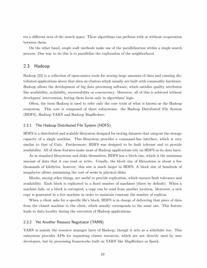
2.3 Hadoop
Hadoop [23] is a collection of open-source tools for storing large amounts of data and running dis-
tributed applications above that data on clusters which usually are built with commodity hardware.
Hadoop allows the development of big data processing software, which satisfies quality attributes
like availability, scalability, recoverability or concurrency. Moreover, all of this is achieved without
developers’ intervention, letting them focus only in algorithms’ logic.
Often, the term Hadoop is used to refer only the core tools of what is known as the Hadoop
ecosystem. This core is composed of three subsystems: the Hadoop Distributed File System
(HDFS), Hadoop YARN and Hadoop MapReduce.
2.3.1 The Hadoop Distributed File System (HDFS)
HDFS is a distributed and scalable filesystem designed for storing datasets that outgrow the storage
capacity of a single machine. This filesystem provides a command-line interface, which is very
similar to that of Unix. Furthermore, HDFS was designed to be fault tolerant and to provide
availability. All of these features make most of Hadoop applications rely on HDFS as its data layer.
As in standard filesystems and disks themselves, HDFS has a block size, which is the minimum
amount of data that it can read or write. Usually, the block size of filesystems is about a few
thousands of kilobytes, however, this size is much larger in HDFS. A block size of hundreds of
megabytes allows minimizing the cost of seeks in physical disks.
Blocks, among other things, are useful to provide replication, which ensures fault tolerance and
availability. Each block is replicated to a fixed number of machines (three by default). When a
machine fails, or a block is corrupted, a copy can be read from another location. Moreover, a new
copy is generated in a live machine in order to maintain constant the number of replicas.
When a client asks for a specific file’s block, HDFS is in charge of delivering that piece of data
from the closest machine to the client, which usually corresponds to the same one. This feature
leads to data locality during the execution of Hadoop applications.
2.3.2 Yet Another Resouce Negotiator (YARN)
YARN is mainly the resource manager layer of Hadoop, though it acts as a scheduler too. This
subsystem provides APIs for requesting cluster resources, which are not directly used by user
developers, but by processing frameworks built on YARN like MapReduce or Spark.
10

An application request in Hadoop includes an amount of memory and a number of CPU cores,
and it also usually includes a locality constraint in order to take the processing to the data and
not the data to the processing. Therefore, if for example, a MapReduce application needs to read
an HDFS block, it can ask YARN for resources in the same machine the block is stored.
YARN is also a job scheduler when there are not enough resources for all requests. It provides
some strategies that the user can use to indicate how applications will have to wait or how resources
will have to be split into shared clusters.
2.3.3 Hadoop MapReduce
At the beginning of Hadoop (I.e., Hadoop version 1), we could only use a distributed implementation
of MapReduce programming model in order to process data stored in HDFS. This implementacion
is known as Hadoop MapReduce, and many other Hadoop tools that came later were built on top
of it. Giraph is one of them, even though it is considered a fake MapReduce application (see section
2.4.5) and new releases include versions that do not depend on MapReduce anymore.
During a MapReduce execution, there are a bunch of mappers, which are small programs in
charge of processing, each of one, a chunk of data in order to produce a partial result. Then,
after other inner phases in the framework, reducers summarize or combine the partial results to
produce the final result. The user developer only has to write the map and reduce functions without
worrying about how the framework parallelizes the computation.
2.4 Giraph
Apache Giraph is a distributed computing framework running above Apache Hadoop that enables
developers to write iterative graph algorithms, which can be executed on large-scale graphs of
millions of vertices [11]. Unlike graph databases systems like Neo4 or Thinkerpop, which are useful
for online transactions, Giraph is an offline computation tool that usually makes analysis over the
whole graph, which can take minutes, hours or days.
Giraph was created as the open-source version of Pregel, a graph processing architecture devel-
oped at Google [10]. Consequently, both systems use a vertex-centric programming model, which
relies on the Bulk Synchronous Parallel (BSP) computation model. In addition to Pregel’s ba-
sic computation model, Giraph offers other features like master computation, sharded aggregators,
edge-oriented input, out-of-core computation, and more. Next, we will describe the most important
of these concepts.
2.4.1 Data Model
A graph in Giraph is represented by a distributed data structure, which follows an edge-cut ap-
proach. That means the vertices of the graph are partitioned and distributed across the processing
11

nodes in the cluster. Furthermore, all the edges in the graph are assigned to their vertex source.
Both vertices and edges have an associated value, which can be an object of any type. Therefore,
a vertex is composed of an ID, a value and a set of outgoing edges, which, at the same time, have
associated values and the ID of their target vertices. As a result, the Giraph’s data model is a
directed graph in which the vertices only have direct access to their outgoing edges and then, if
they need to know the incoming ones, they have to discover them during Giraph’s computation.
In addition to the attributes, vertices behave as illustrated in Listing 2.1.
Listing 2.1: Vertex class
c l a s s Vertex :
map<int , any> edges #1
func t i on voteToHalt ( ) #2
func t i on addEdge ( edge ) #3
func t i on removeEdges ( t a r g e t I d ) #4
#1 The key o f the map i s the t a r g e t vertex ’ s id o f the edge
#2 I s used f o r the ver tex to s i g n a l that i t f i n i s h e d i t s computation
#3 Adds an edge to the ver tex
#4 Removes a l l edges po in t ing to the t a r g e t ver tex
2.4.2 Bulk Synchronous Parallel Model
Bulk Synchronous Parallel is a computation model based on message passing to achieve scalability
for the execution of parallel algorithms in multiple processing nodes. In BSP there are N processing
nodes, which can communicate with each other through a network using for example the Message
Passing Interface (MPI). The input of an algorithm has to be divided across those processing
nodes, and each one has to compute an intermediate solution locally, or at least a part of. At
the end of those computations, which are executed in parallel, the processing nodes exchange their
intermediate results through messages; then, all of them must wait until the other have finished.
When all messages have been delivered, a new iteration starts, in which each processing node has
to compute a new intermediate solution from the previously computed state and the messages that
it received. In Giraph, the waiting phase is known as synchronization barrier and each iteration as
a superstep. The Figure 2.1 1 shows that in Giraph the input partition is made at vertex-level, as
we already explained. Furthermore, Figure 2.1 shows a rough picture of the Giraph computation
model, which we will detail in the next sections.
1Figures 2.1, 2.2, 2.3 and 2.5 are based on illustrations presented in [11].
12

Figure 2.1: Bulk Synchronous Parallel Model
2.4.3 Basic Computation
First of all, it is important to notice that, as developers, Giraph’s users do not have to worry about
distributed systems complexities of the framework. Practically, they only have to deal with the
User Defined Function (UDF), called compute function, that is invoked repeatedly for each vertex,
and which represents the core of the vertex-centric model. In other words, a Giraph programmer
just has to think as a vertex, which has a value that can change over the message exchanges, which
happens over many iterations among its vertex neighbors.
A computation in Giraph is composed of a series of supersteps, which can be seen as the
iterations of an algorithm. At each superstep, a vertex receives messages from other vertices,
which it must process in the next superstep. Moreover, a vertex can access its value and its edges,
change them, and send messages to other vertices. Additionally, a vertex can vote to halt the
computation. Every sent message is delivered to the target vertex at the beginning of the next
superstep. If a vertex vote to halt, it becomes inactive until it receives messages later. An inactive
vertex is not considered in a superstep execution. Furthermore, the computation finishes when
all vertices become inactive. Transitions between supersteps are restricted by a synchronization
barrier, which means that the next superstep cannot begin until all active vertices have been
computed. Thus, Giraph’s computation can be considered a synchronous computation. Figure 2.2
shows the computation of a vertex that receives two messages, updates its value with the largest
one and sends the value to its children.
Processing nodes are responsible to execute the compute function of all the vertices associated
to them. Moreover, at each superstep, they have to deliver the messages produced by their vertices
to the processing nodes containing the target vertices.
13
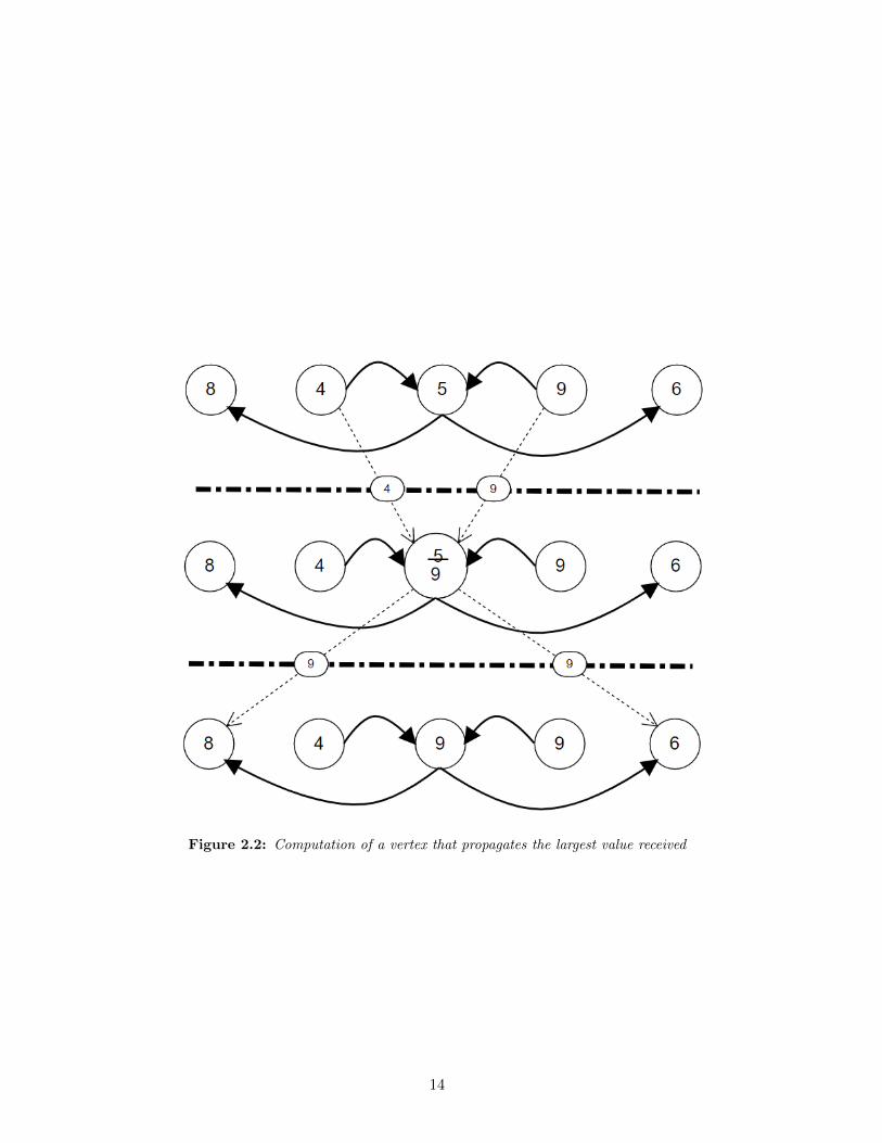
Figure 2.2: Computation of a vertex that propagates the largest value received
14
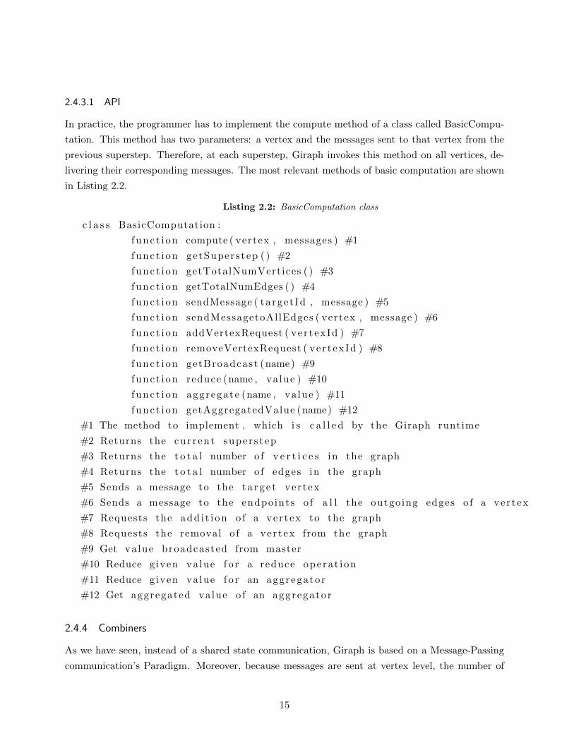
2.4.3.1 API
In practice, the programmer has to implement the compute method of a class called BasicCompu-
tation. This method has two parameters: a vertex and the messages sent to that vertex from the
previous superstep. Therefore, at each superstep, Giraph invokes this method on all vertices, de-
livering their corresponding messages. The most relevant methods of basic computation are shown
in Listing 2.2.
Listing 2.2: BasicComputation class
c l a s s BasicComputation :
func t i on compute ( vertex , messages ) #1
func t i on getSuperstep ( ) #2
func t i on getTotalNumVertices ( ) #3
func t i on getTotalNumEdges ( ) #4
func t i on sendMessage ( ta rge t Id , message ) #5
func t i on sendMessagetoAllEdges ( vertex , message ) #6
func t i on addVertexRequest ( ve r t ex Id ) #7
func t i on removeVertexRequest ( ve r t ex Id ) #8
func t i on getBroadcast (name) #9
func t i on reduce (name , va lue ) #10
func t i on aggregate (name , va lue ) #11
func t i on getAggregatedValue (name) #12
#1 The method to implement , which i s c a l l e d by the Giraph runtime
#2 Returns the cur rent super s tep
#3 Returns the t o t a l number o f v e r t i c e s in the graph
#4 Returns the t o t a l number o f edges in the graph
#5 Sends a message to the t a r g e t ver tex
#6 Sends a message to the endpoints o f a l l the outgoing edges o f a ver tex
#7 Requests the add i t i on o f a ver tex to the graph
#8 Requests the removal o f a ver tex from the graph
#9 Get value broadcasted from master
#10 Reduce g iven value f o r a reduce opera t i on
#11 Reduce g iven value f o r an aggregator
#12 Get aggregated value o f an aggregator
2.4.4 Combiners
As we have seen, instead of a shared state communication, Giraph is based on a Message-Passing
communication’s Paradigm. Moreover, because messages are sent at vertex level, the number of
15

Figure 2.3: Messages reduced by a Max combiner
them can be huge. A combiner is a function that enables to reduce the number of the messages that
are sent to a vertex. Therefore, combiners reduce the network traffic generated between processing
nodes. In practice, a combiner is just a function that combines two messages into one. This function
is known as the combine function. A combiner can be executed before each superstep, but there
is no guaranty about how many times the combiner will be invoked. Figure 2.3 shows how the
number of delivered messages can be reduced from three to one by calling the combine function
two times.
2.4.5 Giraph Architecture
Giraph follows a master-worker pattern in which the processing nodes, which we have talked about,
are the workers. Thus, the main purposes of the workers are both executing the compute function
and exposing the services that allows the direct communication among the workers. On the other
hand, the master processing node has to coordinate the transition of the workers between super-
steps, assign the partitions of nodes to the workers, monitor the health of the workers and run the
master compute code that we will see next.
16
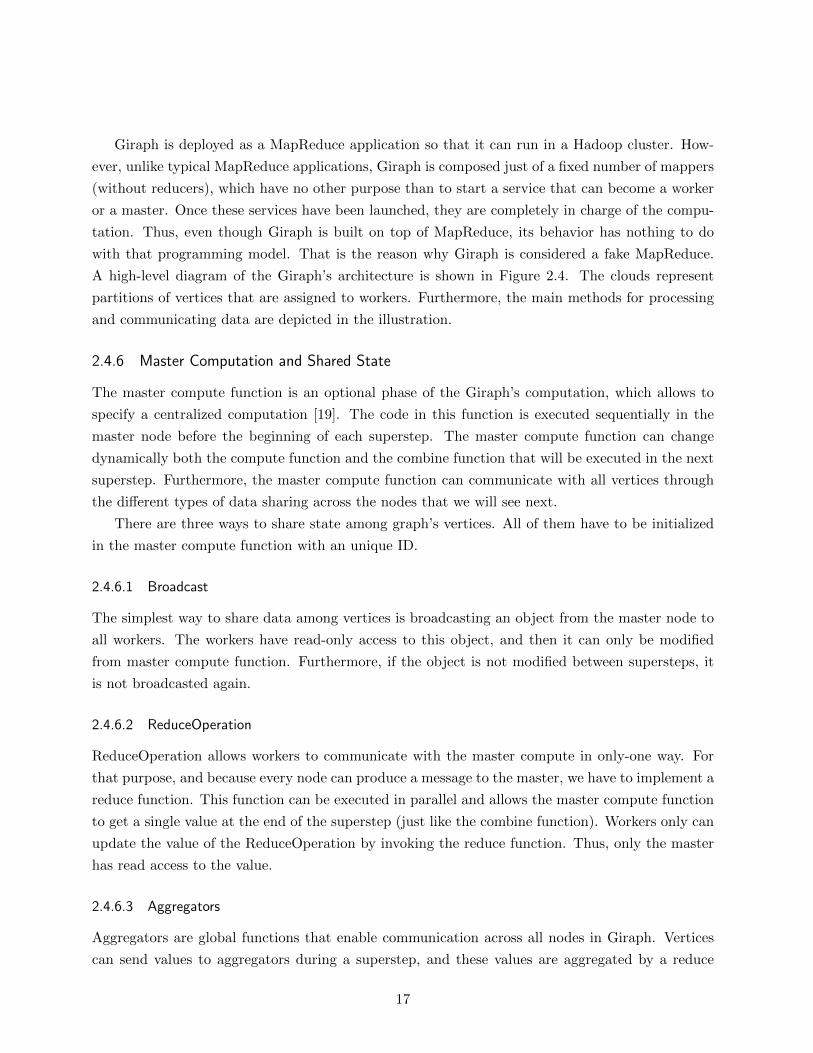
Giraph is deployed as a MapReduce application so that it can run in a Hadoop cluster. How-
ever, unlike typical MapReduce applications, Giraph is composed just of a fixed number of mappers
(without reducers), which have no other purpose than to start a service that can become a worker
or a master. Once these services have been launched, they are completely in charge of the compu-
tation. Thus, even though Giraph is built on top of MapReduce, its behavior has nothing to do
with that programming model. That is the reason why Giraph is considered a fake MapReduce.
A high-level diagram of the Giraph’s architecture is shown in Figure 2.4. The clouds represent
partitions of vertices that are assigned to workers. Furthermore, the main methods for processing
and communicating data are depicted in the illustration.
2.4.6 Master Computation and Shared State
The master compute function is an optional phase of the Giraph’s computation, which allows to
specify a centralized computation [19]. The code in this function is executed sequentially in the
master node before the beginning of each superstep. The master compute function can change
dynamically both the compute function and the combine function that will be executed in the next
superstep. Furthermore, the master compute function can communicate with all vertices through
the different types of data sharing across the nodes that we will see next.
There are three ways to share state among graph’s vertices. All of them have to be initialized
in the master compute function with an unique ID.
2.4.6.1 Broadcast
The simplest way to share data among vertices is broadcasting an object from the master node to
all workers. The workers have read-only access to this object, and then it can only be modified
from master compute function. Furthermore, if the object is not modified between supersteps, it
is not broadcasted again.
2.4.6.2 ReduceOperation
ReduceOperation allows workers to communicate with the master compute in only-one way. For
that purpose, and because every node can produce a message to the master, we have to implement a
reduce function. This function can be executed in parallel and allows the master compute function
to get a single value at the end of the superstep (just like the combine function). Workers only can
update the value of the ReduceOperation by invoking the reduce function. Thus, only the master
has read access to the value.
2.4.6.3 Aggregators
Aggregators are global functions that enable communication across all nodes in Giraph. Vertices
can send values to aggregators during a superstep, and these values are aggregated by a reduce
17
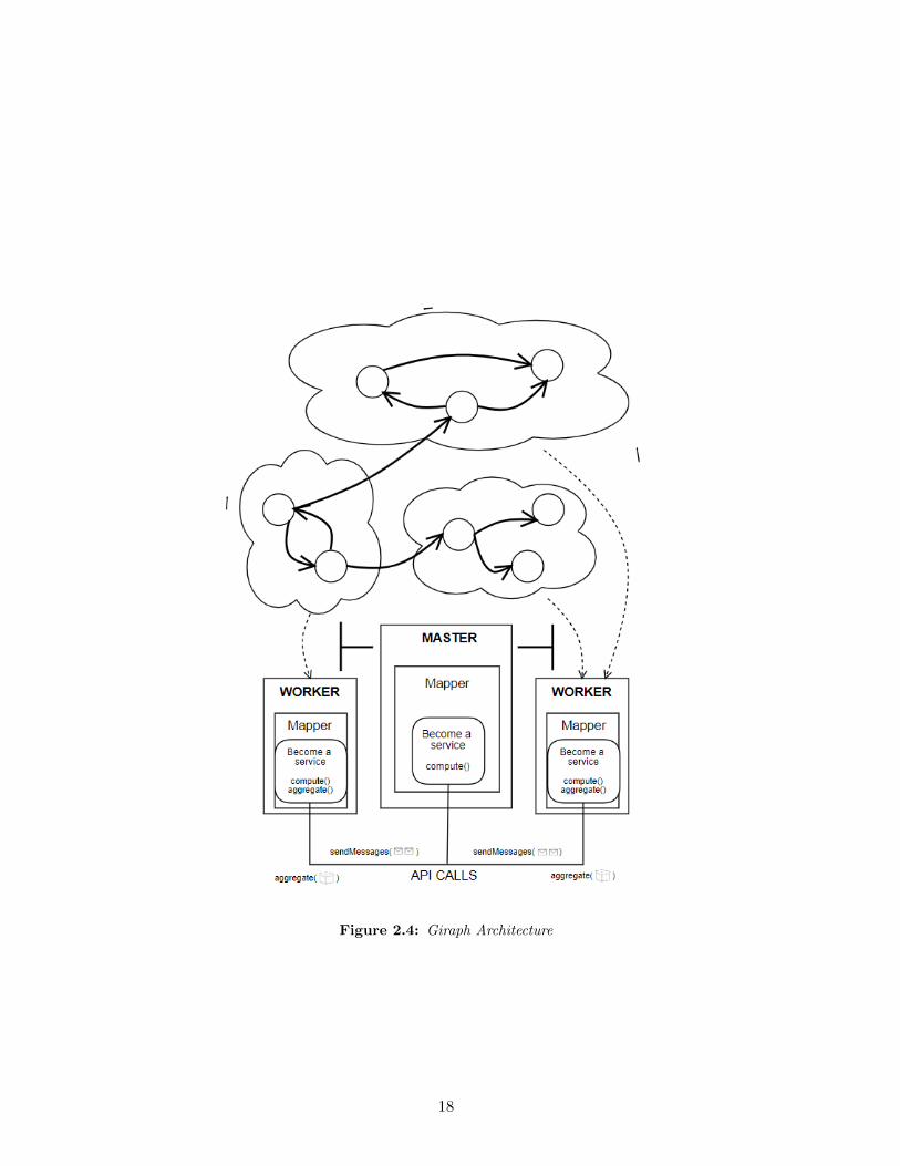
Figure 2.4: Giraph Architecture
18
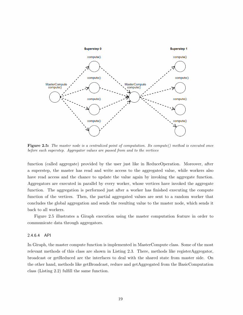
Figure 2.5: The master node is a centralized point of computation. Its compute() method is executed oncebefore each superstep. Aggregator values are passed from and to the vertices
function (called aggregate) provided by the user just like in ReduceOperation. Moreover, after
a superstep, the master has read and write access to the aggregated value, while workers also
have read access and the chance to update the value again by invoking the aggregate function.
Aggregators are executed in parallel by every worker, whose vertices have invoked the aggregate
function. The aggregation is performed just after a worker has finished executing the compute
function of the vertices. Then, the partial aggregated values are sent to a random worker that
concludes the global aggregation and sends the resulting value to the master node, which sends it
back to all workers.
Figure 2.5 illustrates a Giraph execution using the master computation feature in order to
communicate data through aggregators.
2.4.6.4 API
In Giraph, the master compute function is implemented in MasterCompute class. Some of the most
relevant methods of this class are shown in Listing 2.3. There, methods like registerAggregator,
broadcast or getReduced are the interfaces to deal with the shared state from master side. On
the other hand, methods like getBroadcast, reduce and getAggregated from the BasicComputation
class (Listing 2.2) fulfill the same function.
19
Listing 2.3: MasterComputation class
c l a s s MasterCompute :f unc t i on compute ( ) #1func t i on getSuperstep ( ) #2func t i on getTotalNumVertices ( ) #3func t i on getTotalNumEdges ( ) #4func t i on r e g i s t e r A g g r e g a t o r (name) #5func t i on reg i s terReduceOperadion (name) #6func t i on broadcast ( ob j e c t ) #7func t i on haltComputation ( ) #8func t i on setComputation ( c l a s s ) #9func t i on setCombiner ( c l a s s ) #10func t i on getReduced (name) #11func t i on getAggregatedValue (name) #12
#1 The method to implement , which i s c a l l e d by the Giraph runtime#2 Returns the cur rent super s tep#3 Returns the t o t a l number o f v e r t i c e s in the graph#4 Returns the t o t a l number o f edges in the graph#5 Reg i s t e r a aggregator#6 Reg i s t e r a reduce opera t i on#7 Sends an ob j e c t to the workers#8 Halts the computation#9 Sets the compute func t i on f o r the next super s t ep#10 Sets the combine func t i on f o r the next super s t ep#11 Get reduced value o f an reduceOperat ion#12 Get aggregated value o f an aggregator
20

Chapter 3
Understanding the Giraph Computation Model
In order to achieve a better understanding of the programming model and show the execution flow
of Giraph, in this chapter we propose a couple of small sub-problems related to the problem tackled
in this thesis, and we describe in detail how these problems can be solved in Giraph.
3.1 A simple problem
Given a tree whose vertices store a numeric value, for each vertex, find the largest value of the
subtree in which it is the root. At the end of the computation the value for the leaves should be
their original values, whereas for the root, it should be the largest value of the entire tree. Figure
3.1 shows the result of the computation given a particular input graph.
A strategy to solve the problem using the vertex-centric programming paradigm is the following:
for every vertex, propagate upwards its value (that is sending a message to its parent) and wait
until a new larger value arrives at it in a message form. As a consequence, the vertex value has
to be updated and propagated upwards again. When no messages are sent, the computation is
(a) Problem’s input (b) Problem’s solution
Figure 3.1: A simple problem’s solution
21
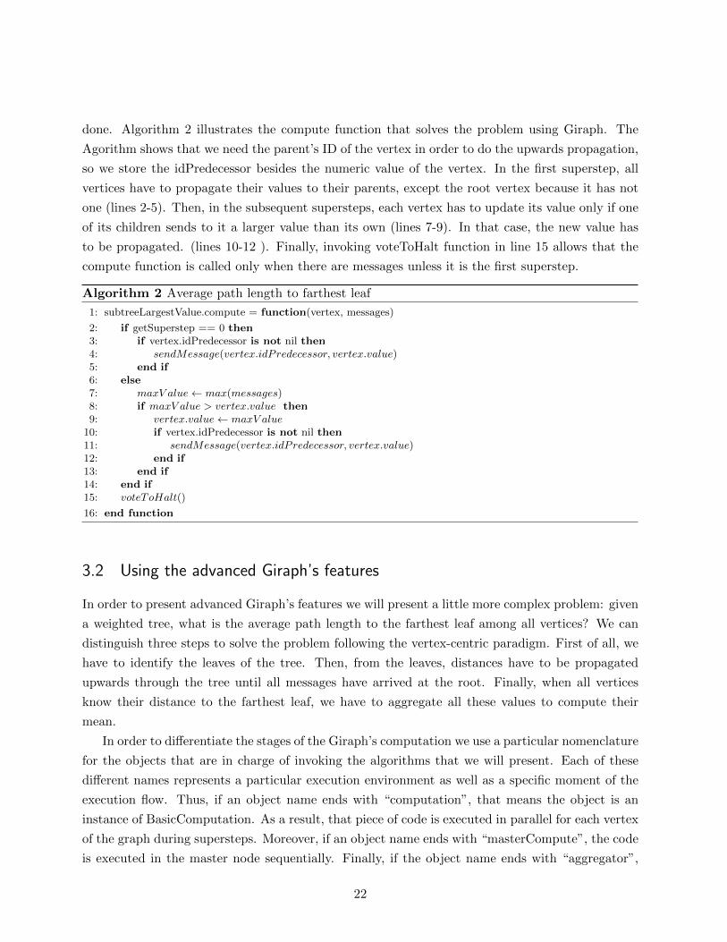
done. Algorithm 2 illustrates the compute function that solves the problem using Giraph. The
Agorithm shows that we need the parent’s ID of the vertex in order to do the upwards propagation,
so we store the idPredecessor besides the numeric value of the vertex. In the first superstep, all
vertices have to propagate their values to their parents, except the root vertex because it has not
one (lines 2-5). Then, in the subsequent supersteps, each vertex has to update its value only if one
of its children sends to it a larger value than its own (lines 7-9). In that case, the new value has
to be propagated. (lines 10-12 ). Finally, invoking voteToHalt function in line 15 allows that the
compute function is called only when there are messages unless it is the first superstep.
Algorithm 2 Average path length to farthest leaf
1: subtreeLargestValue.compute = function(vertex, messages)
2: if getSuperstep == 0 then3: if vertex.idPredecessor is not nil then4: sendMessage(vertex.idPredecessor, vertex.value)5: end if6: else7: maxV alue← max(messages)8: if maxV alue > vertex.value then9: vertex.value← maxV alue
10: if vertex.idPredecessor is not nil then11: sendMessage(vertex.idPredecessor, vertex.value)12: end if13: end if14: end if15: voteToHalt()
16: end function
3.2 Using the advanced Giraph’s features
In order to present advanced Giraph’s features we will present a little more complex problem: given
a weighted tree, what is the average path length to the farthest leaf among all vertices? We can
distinguish three steps to solve the problem following the vertex-centric paradigm. First of all, we
have to identify the leaves of the tree. Then, from the leaves, distances have to be propagated
upwards through the tree until all messages have arrived at the root. Finally, when all vertices
know their distance to the farthest leaf, we have to aggregate all these values to compute their
mean.
In order to differentiate the stages of the Giraph’s computation we use a particular nomenclature
for the objects that are in charge of invoking the algorithms that we will present. Each of these
different names represents a particular execution environment as well as a specific moment of the
execution flow. Thus, if an object name ends with “computation”, that means the object is an
instance of BasicComputation. As a result, that piece of code is executed in parallel for each vertex
of the graph during supersteps. Moreover, if an object name ends with “masterCompute”, the code
is executed in the master node sequentially. Finally, if the object name ends with “aggregator”,
22
“combiner”, or “reducer” it refers to an aggregator, a combiner and a reduce operation respectively.
Their respective “aggregate”, “combine” and “reduce” functions are executed by the workers just
after they have computed all their vertices during the superstep.
3.2.1 Data model
We defined the vertex value as an object with two attributes: a number that represents the distance
to the farthest leaf, which we call backwards distance or simply b; and the ID of the vertex
predecessor. We have to remember the vertex only has access to their outgoing edges, and because
we need to propagate messages upwards, it is necessary that each vertex knows the ID of its unique
predecessor. Only the root vertex does not have a predecessor. On the other hand, the edge value
is a number that represents the distance between nodes.
3.2.2 Master compute
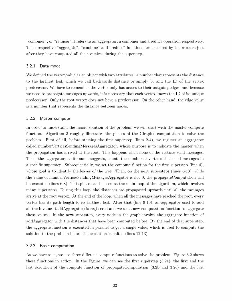
In order to understand the macro solution of the problem, we will start with the master compute
function. Algorithm 3 roughly illustrates the phases of the Giraph’s computation to solve the
problem. First of all, before starting the first superstep (lines 2-4), we register an aggregator
called numberVerticesSendingMessagesAggregator, whose purpose is to indicate the master when
the propagation has arrived at the root. This happens when none of the vertices send messages.
Thus, the aggregator, as its name suggests, counts the number of vertices that send messages in
a specific superstep. Subsequentially, we set the compute function for the first superstep (line 4),
whose goal is to identify the leaves of the tree. Then, on the next supersteps (lines 5-13), while
the value of numberVerticesSendingMessagesAggregator is not 0, the propagateComputation will
be executed (lines 6-8). This phase can be seen as the main loop of the algorithm, which involves
many supersteps. During this loop, the distances are propagated upwards until all the messages
arrive at the root vertex. At the end of the loop, when all the messages have reached the root, every
vertex has its path length to its farthest leaf. After that (line 9-10), an aggregator used to add
all the b values (addAggregator) is registered and we set a new computation function to aggregate
those values. In the next superstep, every node in the graph invokes the aggregate function of
addAggregator with the distances that have been computed before. By the end of that superstep,
the aggregate function is executed in parallel to get a single value, which is used to compute the
solution to the problem before the execution is halted (lines 12-13).
3.2.3 Basic computation
As we have seen, we use three different compute functions to solve the problem. Figure 3.2 shows
these functions in action. In the Figure, we can see the first superstep (3.2a), the first and the
last execution of the compute function of propagateComputation (3.2b and 3.2c) and the last
23
Algorithm 3 Average path length to farthest leaf
1: averagePathLengthToFarthestLeafMasterCompute.compute = function()
2: if getSuperstep() == 0 then3: registerReduceOperation(“numberV erticesSendingMessagesAggregator”)4: setComputation(leafIdentifyComputation)5: else6: if numberVerticesSendingMessagesAggregator.value is not 0 then7: setComputation(propagateComputation)8: else if meanAggregator is nil then9: registerAggregator(“addAggregator”)
10: setComputation(addAggregateComputation)11: else12: finalResult← addAggregator.value/getTotalNumV ertices()13: haltComputation()14: end if15: end if16: end function
superstep of the whole computation (3.2d). Moreover, Algorithms 4, 5 and 6, show the details of
the implementation of each one of these functions.
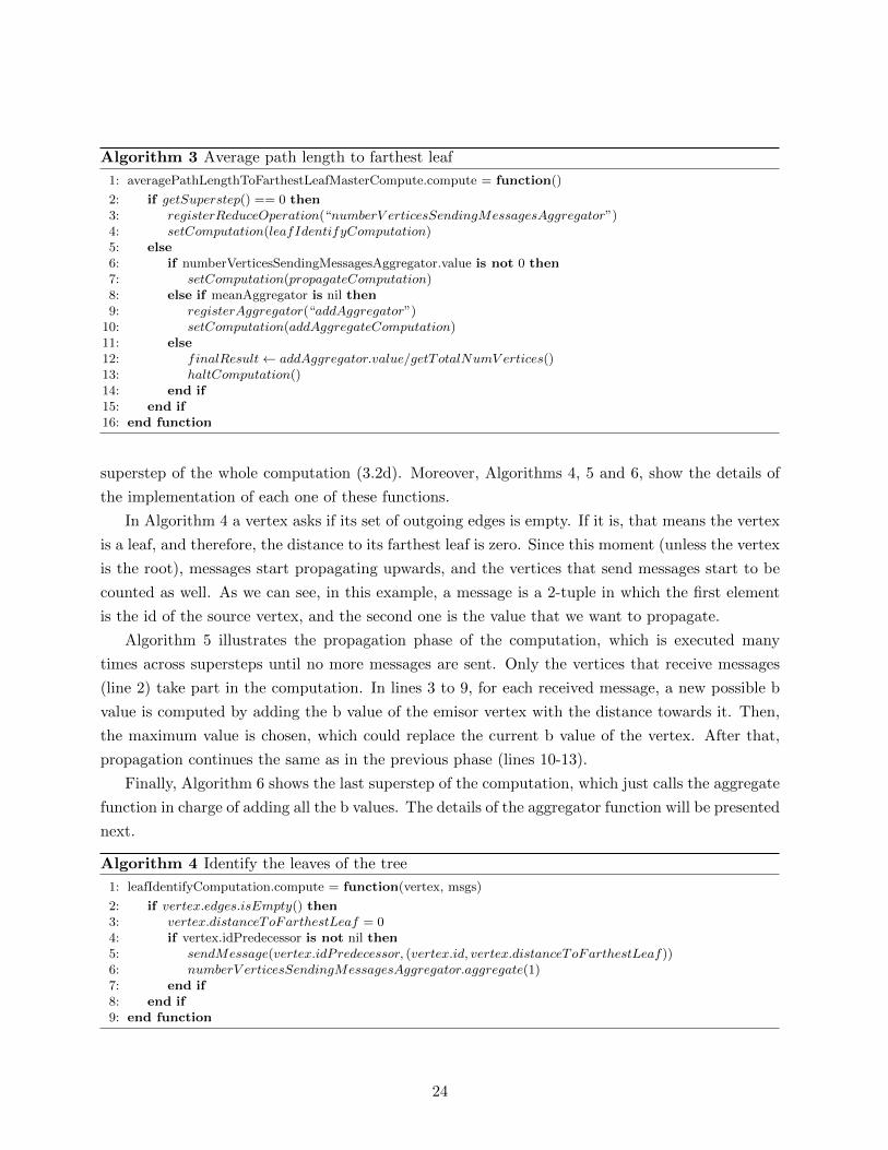
In Algorithm 4 a vertex asks if its set of outgoing edges is empty. If it is, that means the vertex
is a leaf, and therefore, the distance to its farthest leaf is zero. Since this moment (unless the vertex
is the root), messages start propagating upwards, and the vertices that send messages start to be
counted as well. As we can see, in this example, a message is a 2-tuple in which the first element
is the id of the source vertex, and the second one is the value that we want to propagate.
Algorithm 5 illustrates the propagation phase of the computation, which is executed many
times across supersteps until no more messages are sent. Only the vertices that receive messages
(line 2) take part in the computation. In lines 3 to 9, for each received message, a new possible b
value is computed by adding the b value of the emisor vertex with the distance towards it. Then,
the maximum value is chosen, which could replace the current b value of the vertex. After that,
propagation continues the same as in the previous phase (lines 10-13).
Finally, Algorithm 6 shows the last superstep of the computation, which just calls the aggregate
function in charge of adding all the b values. The details of the aggregator function will be presented
next.
Algorithm 4 Identify the leaves of the tree
1: leafIdentifyComputation.compute = function(vertex, msgs)
2: if vertex.edges.isEmpty() then3: vertex.distanceToFarthestLeaf = 04: if vertex.idPredecessor is not nil then5: sendMessage(vertex.idPredecessor, (vertex.id, vertex.distanceToFarthestLeaf))6: numberV erticesSendingMessagesAggregator.aggregate(1)7: end if8: end if9: end function
24

(a) Identify the leaves of the tree (b) Propagate the distances to farthest leaves (first itera-tion)
(c) Propagate the distances to farthest leaves (last itera-tion) (d) Aggregate the final distances
Figure 3.2: Supersteps to find the average path length to farthest leaf
Algorithm 5 Propagate the distances to farthest leaves
1: propagateComputation.compute = function(vertex, messages)
2: if not msg.isEmpty() then3: maxPossibleNewB ← 04: for msg in messages do5: maxPossibleNewB ← vertex.edges.get(msg[0]) +msg[1]6: if maxPossibleNewB > vertex.distanceToFarthestLeaf then7: vertex.distanceToFarthestLeaf ← maxPossibleNewB8: end if9: end for
10: if vertex.idPredecessor is not nil then11: sendMessage(vertex.idPredecessor, (vertex.id, vertex.distanceToFarthestLeaf))12: numberV erticesSendingMessagesAggregator.aggregate(1)13: end if14: end if15: end function
25
Algorithm 6 Aggregate the final distances
1: addAggregateComputation.compute = function(vertex, messages)
2: addAggregator.aggregate(vertex.distanceToFarthestLeaf)
3: end function
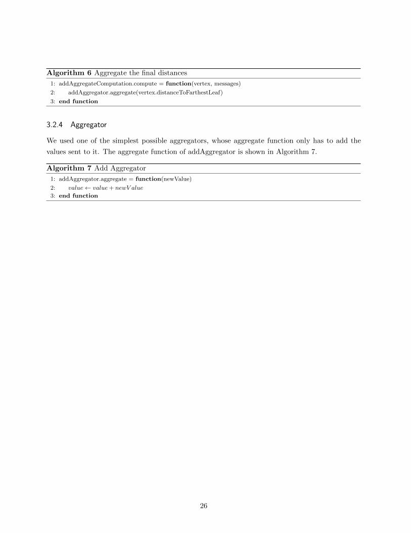
3.2.4 Aggregator
We used one of the simplest possible aggregators, whose aggregate function only has to add the
values sent to it. The aggregate function of addAggregator is shown in Algorithm 7.
Algorithm 7 Add Aggregator
1: addAggregator.aggregate = function(newValue)
2: value← value+ newV alue
3: end function
26
Chapter 4
The Global Design Strategy Exploiting Giraph
In this chapter, based on the understanding of the Giraph computation model presented in the
previous chapter, we illustrate our strategy and discuss the ideas that led us to work on this
project.
4.1 An Iterated Local Search to solve RDCMST
Arbelaez et al. proposed an ILC to solve the RDCMST problem. This thesis is born from the idea
of distributing that strategy in order to explore the possibilities and also the limitations of using
the computational model of Giraph to solve this kind of problems.
4.1.1 The problem
The Minimum Spanning Tree is one of those problems in which by adding a small constraint it
goes from a relatively easy problem to a monster of complexity. In the classic MST, given a graph,
the goal is to find a tree that contains all vertices, minimizing the overall edge’s weight. We can
solve this in linear time. However, if we select a vertex as the root, and constrain the distance from
that root to any other vertex in the tree, the problem becomes NP-Hard. Next, we will describe
the approach Arbelaez et al. follow to tackle the Rooted Distance-Constraint Minimum Spanning
Tree.
4.1.2 The sequential algorithm
Sophisticated exhaustive approaches like the Simplex Method, hardly can handle graphs of hundreds
of vertices [1]. Therefore, the most straightforward alternative is a heuristic method to approximate
a solution to the problem. The algorithm presented in this section is a Local Search in which an
initial suboptimal solution is improved step by step.
In a nutshell, given a tree, which is a partial solution to the problem, the local search consists
of selecting randomly one vertex of the tree, removing it, reinserting it in the best location and
27
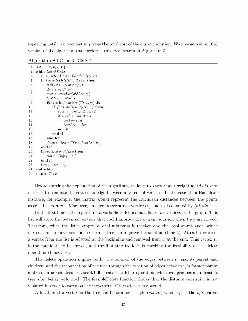
repeating until no movement improves the total cost of the current solution. We present a simplified
version of the algorithm that performs this local search in Algorithm 8.
Algorithm 8 LC for RDCMST
1: list← {vi|vi ∈ V }2: while list 6= ∅ do3: vj ← selectV ertexRandomly(list)4: if feasibleDelete(vj , T ree) then5: oldLoc← location(vj)6: delete(vj , T ree)7: cost← costLoc(oldLoc, vj)8: bestLoc← oldLoc9: for loc in locations(Tree, vj) do
10: if feasibleInsert(loc, vj) then11: cost′ ← costLoc(loc, vj)12: if cost′ < cost then13: cost← cost′
14: bestLoc← loc15: end if16: end if17: end for18: Tree← insert(Tree, bestLoc, vj)19: end if20: if bestLoc 6= oldLoc then21: list← {vi|vi ∈ V }22: end if23: list← list− vj24: end while25: return Tree
Before starting the explanation of the algorithm, we have to know that a weight matrix is kept
in order to compute the cost of an edge between any pair of vertices. In the case of an Euclidean
instance, for example, the matrix would represent the Euclidean distances between the points
assigned as vertices. Moreover, an edge between two vertices vj and vk is denoted by 〈vj, vk〉.In the first line of the algorithm, a variable is defined as a list of all vertices in the graph. This
list will store the potential vertices that could improve the current solution when they are moved.
Therefore, when the list is empty, a local minimum is reached and the local search ends, which
means that no movement in the current tree can improve the solution (Line 2). At each iteration,
a vertex from the list is selected at the beginning and removed from it at the end. This vertex vj
is the candidate to be moved, and the first step to do it is checking the feasibility of the delete
operation (Lines 3-4).
The delete operation implies both: the removal of the edges between vj and its parent and
children; and the reconnection of the tree through the creation of edges between vj ’s former parent
and vj ’s former children. Figure 4.1 illustrates the delete operation, which can produce an unfeasible
tree after being performed. The feasibleDelete function checks that the distance constraint is not
violated in order to carry on the movement. Otherwise, it is aborted.
A location of a vertex in the tree can be seen as a tuple (vpj , Sj) where vpj is the vj ’s parent
28
and Sj are the vj children. Then, immediately before the delete operation is performed, the current
location of vj is saved in a variable (Line 5). Furthermore, the costLoc function, which computes
the overall cost of the tree as if a vertex were inserted at a specified location, calculates the cost
of the current solution, and it is stored in the cost variable. Also, the bestLoc variable, that stores
the best location for vj is initialized with its former location in line 7.
A vertex can be inserted as a new leaf child for another vertex or in the middle of an existing
edge in the tree (Figure 4.8). The first scenario only implies the creation of an edge between
any new vj ’s parent vnewpj and it 〈vnewpj , vj〉. The second one is achieved by removing the edge
between two vertices 〈vm, vn〉. and creating the edges 〈vm, vj〉 and 〈vj , vn〉. Consequently, the
function locations returns all possible locations in the tree for vertex vj following the scenarios
mentioned above. Then, we evaluate each location, looking for the least expensive and verifying
its feasibility (Lines 9-17).
Finally, once all locations have been considered, the insert operation is performed with the
best location. Moreover, if a movement was actually accomplished, all vertices are reintroduced
to the list given that with the new solution’s conditions, their movements could now produce
improvements (Lines 20-22).
The time complexity of a movement is O(n), and it is always determined by the best location
operation, which has to iterate over all vertices in order to check all possible locations. The other
operation such as the insert operation, delete operation or checking feasibility in the worst case
have to go through the complete set of vertices, but usually (depending on the implementation)
the complexity is less than that.
Algorithm 8 is wrapped in the template of a general ILC illustrated in Algortithm 1. In our
case, the perturbation function performs a series of random movements without the best location
heuristic, which means they only check the feasibility of the output.
4.1.3 Towards a parallel solution
To the best of our knowledge, there is no parallel solution for the RDCMST problem. However,
nowadays computer hardware is naturally parallel [12], and therefore, parallel algorithms are needed
in order to exploit it. Moreover, big data is a reality [23], and thus, the design of distributed
algorithms is a necessity.
As we showed in chapter 2, the different approaches to solve the problem deal only with hundreds
or a few thousands of vertices at best. Furthermore, in experiments performed on real instances
of the problem, Arbelaez et al. reached ten thousand vertices at solving the more general prob-
lem edge-disjoint rooted distance-constrained minimum spanning tree (ERDCMS), which includes
solving RDCMST. Our main goal is to present a strategy that allows for handling much bigger
instances.
The most natural approach to parallelize Algorithm 8 is splitting neighborhood exploration
29

Figure 4.1
(a) As a new leaf child for another vertex (b) In the middle of an existing edge
Figure 4.2: Insert operation’s scenarios
into independent tasks, each one in charge of evaluating different locations. In code, this means
using a “parallel for” in line 9 of the algorithm. Nevertheless, some other operations inside the
local search such as checking feasibility can take advantage of parallelization. In the next chapter,
we propose a strategy to parallelize almost entirely Algorithm 8 in a distributed system following
30
Pregel’s computing paradigm [10].
4.2 Using Giraph to Solve RDCMST: A Complete Solution
This section presents our main contribution in this thesis, which is the design of a strategy to solve
the RDCMST problem following Pregel’s model of computation. This strategy is based on the
algorithm introduced in the previous section.
We have called ‘movement’ to a complete iteration of Algorithm 8. A movement can be seen as
a sequence of two primary operations: the delete operation and the insert operation. In the first
one, a vertex is selected and removed from the tree; in the second one, the algorithm chooses the
best location for the removed vertex, and it is reinserted there.
We implement a movement in Giraph as a sequence of five supersteps: roughly, the first two
correspond to the delete operation and the remaining ones to the insert operation. Repetitions of
these five supersteps constitute the iterative local search to solve the problem. Even though this
correspondence may seem pretty straightforward, the distribution across supersteps of secondary
operations in charge of dealing with the prerequisites and consequences of the principal operations
(in terms of the vertices’ state) is a little more complex. However, we will present the strategy
structured in two sections corresponding to the two main operations of the movement and for each
of them, we will have subsections explaining separately the secondary operations.
In this section, we will present our solution’s data model in Giraph, then an overview of the
solution presented through the details of the master compute function’s implementation. Finally,
we will show the design of a complete movement using Giraph in two sub-sections, one for the
delete operation and the other one for the insert operation.
In addition to this chapter, Appendix A presents a graphical description of a complete move-
ment, including all its different scenarios. That section can be used as a complementary tool to
understand the strategy.
4.2.1 Data model
We defined the vertex value as a data structure implemented in the VertexValue class (Listing 4.2)
whose fields are presented next. The examples presented on each field are explained considering
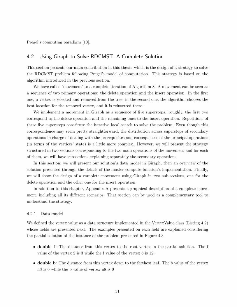
the partial solution of the instance of the problem presented in Figure 4.3
• double f : The distance from this vertex to the root vertex in the partial solution. The f
value of the vertex 2 is 3 while the f value of the vertex 8 is 12.
• double b: The distance from this vertex down to the farthest leaf. The b value of the vertex
n3 is 6 while the b value of vertex n8 is 0
31

Figure 4.3: Partial solution for RDCMST problem
• map < int, enum > positions: Relate the vertices of the tree with the position of this
vertex with respect to it. The indexes correspond to the ids of all the graph’s vertices. The
values are Enums with three possible values that indicate if, for the corresponding vertex to
the index, this vertex is an ancestor, a descendant or neither. For example, the map of vertex
3 would look like the structure presented in Listing 4.1
• map < int, double > distances: relate the vertices of the tree with the distances of this
vertex to them. In this map, the indexes are the same of positions but the values are the
distance that there would be if an edge connected directly this vertex to the corresponding
vertex in the index.
• int parentId: the ID of the unique parent of this vertex. The parentId of vertex n3 is 2
and the parentId of vertex n4 is 6. The only vertex that doesn’t have a parent is the facility
vertex.
• double olfF: the value of f just after the previous movement was completed.
• double oldB: the value of b just after the previous movement was completed.
• double partialBestLocationCost: temporarily stores the cost of inserting the selected
vertex as a child of this vertex.
32
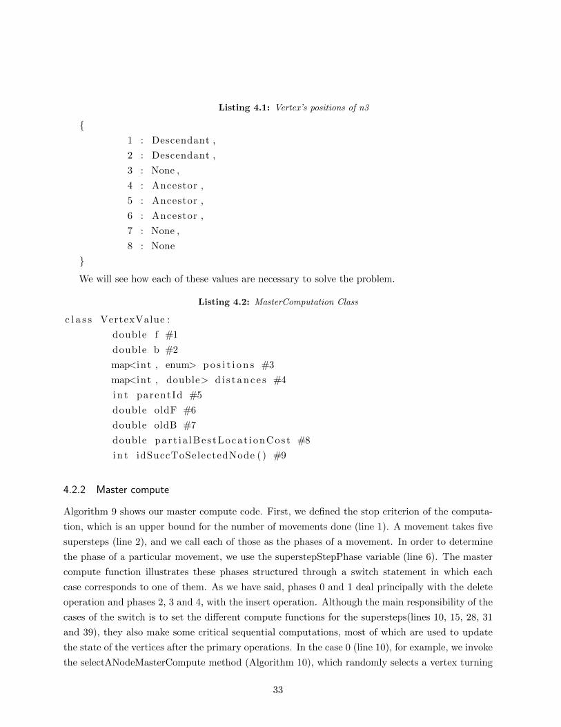
Listing 4.1: Vertex’s positions of n3
{1 : Descendant ,
2 : Descendant ,
3 : None ,
4 : Ancestor ,
5 : Ancestor ,
6 : Ancestor ,
7 : None ,
8 : None
}
We will see how each of these values are necessary to solve the problem.
Listing 4.2: MasterComputation Class
c l a s s VertexValue :
double f #1
double b #2
map<int , enum> p o s i t i o n s #3
map<int , double> d i s t a n c e s #4
i n t parentId #5
double oldF #6
double oldB #7
double par t i a lBes tLoca t i onCos t #8
i n t idSuccToSelectedNode ( ) #9
4.2.2 Master compute
Algorithm 9 shows our master compute code. First, we defined the stop criterion of the computa-
tion, which is an upper bound for the number of movements done (line 1). A movement takes five
supersteps (line 2), and we call each of those as the phases of a movement. In order to determine
the phase of a particular movement, we use the superstepStepPhase variable (line 6). The master
compute function illustrates these phases structured through a switch statement in which each
case corresponds to one of them. As we have said, phases 0 and 1 deal principally with the delete
operation and phases 2, 3 and 4, with the insert operation. Although the main responsibility of the
cases of the switch is to set the different compute functions for the supersteps(lines 10, 15, 28, 31
and 39), they also make some critical sequential computations, most of which are used to update
the state of the vertices after the primary operations. In the case 0 (line 10), for example, we invoke
the selectANodeMasterCompute method (Algorithm 10), which randomly selects a vertex turning
33
it into a global variable. Moreover, the method creates a couple of variables related to the state
update needed after the delete operation.
During the descriptions of each of the five supersteps presented next, we will see in detail all
the cases of the master compute function.
4.2.3 Delete operation
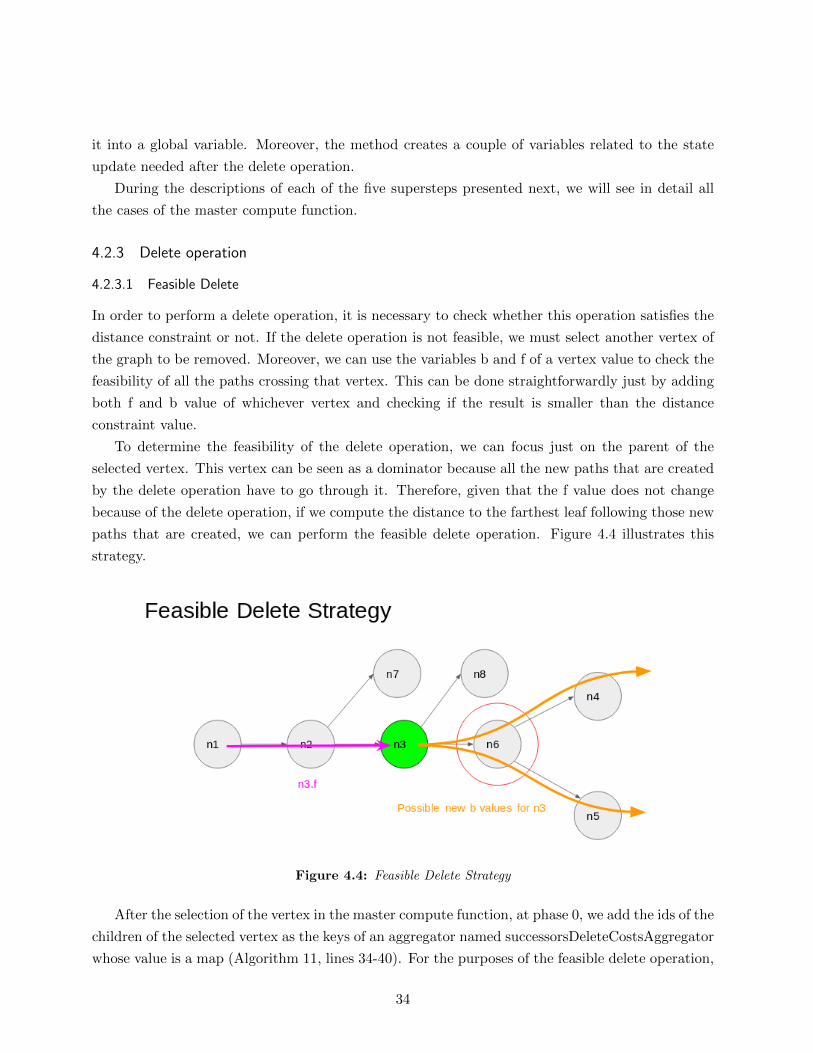
4.2.3.1 Feasible Delete
In order to perform a delete operation, it is necessary to check whether this operation satisfies the
distance constraint or not. If the delete operation is not feasible, we must select another vertex of
the graph to be removed. Moreover, we can use the variables b and f of a vertex value to check the
feasibility of all the paths crossing that vertex. This can be done straightforwardly just by adding
both f and b value of whichever vertex and checking if the result is smaller than the distance
constraint value.
To determine the feasibility of the delete operation, we can focus just on the parent of the
selected vertex. This vertex can be seen as a dominator because all the new paths that are created
by the delete operation have to go through it. Therefore, given that the f value does not change
because of the delete operation, if we compute the distance to the farthest leaf following those new
paths that are created, we can perform the feasible delete operation. Figure 4.4 illustrates this
strategy.
Figure 4.4: Feasible Delete Strategy
After the selection of the vertex in the master compute function, at phase 0, we add the ids of the
children of the selected vertex as the keys of an aggregator named successorsDeleteCostsAggregator
whose value is a map (Algorithm 11, lines 34-40). For the purposes of the feasible delete operation,
34
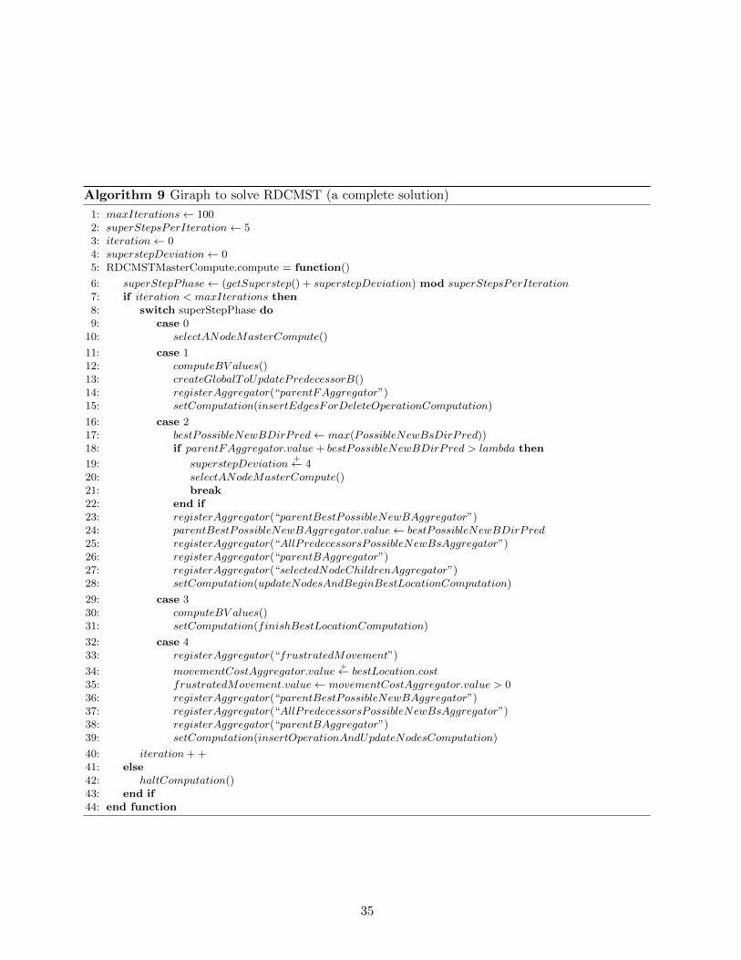
Algorithm 9 Giraph to solve RDCMST (a complete solution)
1: maxIterations← 1002: superStepsPerIteration← 53: iteration← 04: superstepDeviation← 05: RDCMSTMasterCompute.compute = function()
6: superStepPhase← (getSuperstep() + superstepDeviation) mod superStepsPerIteration7: if iteration < maxIterations then8: switch superStepPhase do9: case 0
10: selectANodeMasterCompute()
11: case 112: computeBV alues()13: createGlobalToUpdatePredecessorB()14: registerAggregator(“parentFAggregator”)15: setComputation(insertEdgesForDeleteOperationComputation)
16: case 217: bestPossibleNewBDirPred← max(PossibleNewBsDirPred))18: if parentFAggregator.value+ bestPossibleNewBDirPred > lambda then
19: superstepDeviation+← 4
20: selectANodeMasterCompute()21: break22: end if23: registerAggregator(“parentBestPossibleNewBAggregator”)24: parentBestPossibleNewBAggregator.value← bestPossibleNewBDirPred25: registerAggregator(“AllPredecessorsPossibleNewBsAggregator”)26: registerAggregator(“parentBAggregator”)27: registerAggregator(“selectedNodeChildrenAggregator”)28: setComputation(updateNodesAndBeginBestLocationComputation)
29: case 330: computeBV alues()31: setComputation(finishBestLocationComputation)
32: case 433: registerAggregator(“frustratedMovement”)
34: movementCostAggregator.value+← bestLocation.cost
35: frustratedMovement.value← movementCostAggregator.value > 036: registerAggregator(“parentBestPossibleNewBAggregator”)37: registerAggregator(“AllPredecessorsPossibleNewBsAggregator”)38: registerAggregator(“parentBAggregator”)39: setComputation(insertOperationAndUpdateNodesComputation)
40: iteration+ +41: else42: haltComputation()43: end if44: end function
35

Algorithm 10 Selection of a vertex (master compute 0)
1: selectANodeMasterCompute = function()
2: selectedNode← selectRamdomlyANode()3: broadcast(“selectedNodeAggregator”, selectedNode)4: registerReducer(“deleteCostForSuccessorsReduceOperation”)5: registerAggregator(“movementCostAggregator”)6: setComputation(removeEdgesForDeleteOperationComputation)
7: end function
we only need those keys, though the aggregator accomplishes another function. These ids are useful
to identify the new paths that would be created because of the delete operation. Then, in the case
1 of the master compute function, we create a new aggregator named parentPossibleNewBsAggre-
gator, which is a map that shares the same keys of successorsDeleteCostsAggregator, (Algorithm
9, line 13; Algorithm 13) and the same aggregate function (Algorithm 14). Each element’s value of
this aggregator is the distance from the selected vertex’s parent to the farthest leaf in the subtree
whose root is the element’s key. Thus, in phase 1, the parent of the selected vertex has to provide
to parentPossibleNewBsAggregator the cost of connecting it with all the children of the selected
vertex (Algorithm 12, lines 16-25). At the same time, the children of the selected vertex have to
add its b values in the same aggregator in the corresponding key (Algorithm 12, lines 30-32). As
a result, at the end of the phase, parentPossibleNewBsAggregator contains the distances to the
farthest leaves from the the selected vertex’s parent following the paths that go through each of the
selected vertex’s children. Those are the possible b values of the selected vertex’s parent that really
could break the distance constraint. Additionally, in phase 1, the selected vertex’s parent stores
its f value in a aggregator (Algorithm 12, line 27). This is done in order to perform the feasible
delete operation in the next invocation of the master compute function so that we do not need to
wait until next superstep. Therefore, in the case 2 of master compute function, we are ready to
compute the feasible delete operation. First, we have to find the maximum value of parentPossi-
bleNewBsAggregator, and then check if that value plus parentFAggregator value is higher than the
distance constraint value. If this is so, we have to skip the next phases of the current movement
and a complete new movement has to start in the next superstep (Algorithm 9, lines 17-21).
4.2.3.2 Delete consequences (update of graph’s state)
The delete operation has an impact over the graph’s state. The most noticeable change is the
topological one, which implies the addition and removal of edges that we have seen in Section 4.1.
However, that is not the only graph’s state change after the delete operation. We keep some crucial
variables in each vertex that must be updated: The f and b variables that allow us to check easily
the feasibility of the distance constraint and the position array that allows vertices to know their
positions with respect to any other vertex in order to perform particular tasks that depend on that.
Those variables have to be updated after both delete and insert operations. The update of those
36
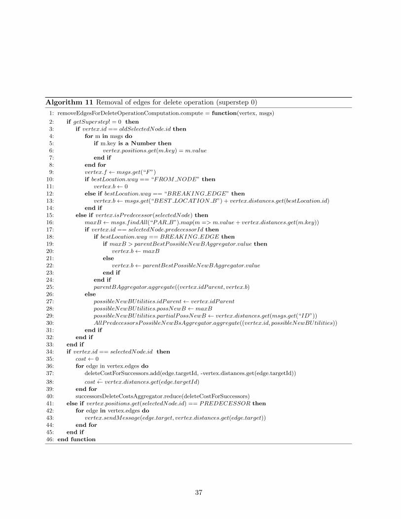
Algorithm 11 Removal of edges for delete operation (superstep 0)
1: removeEdgesForDeleteOperationComputation.compute = function(vertex, msgs)
2: if getSuperstep! = 0 then3: if vertex.id == oldSelectedNode.id then4: for m in msgs do5: if m.key is a Number then6: vertex.positions.get(m.key) = m.value7: end if8: end for9: vertex.f ← msgs.get(“F”)
10: if bestLocation.way == “FROM NODE” then11: vertex.b← 012: else if bestLocation.way == “BREAKING EDGE” then13: vertex.b← msgs.get(“BEST LOCATION B”) + vertex.distances.get(bestLocation.id)14: end if15: else if vertex.isPredecessor(selectedNode) then16: maxB ← msgs.findAll(“PAR B”).map(m => m.value+ vertex.distances.get(m.key))17: if vertex.id == selectedNode.predecessorId then18: if bestLocation.way == BREAKING EDGE then19: if maxB > parentBestPossibleNewBAggregator.value then20: vertex.b← maxB21: else22: vertex.b← parentBestPossibleNewBAggregator.value23: end if24: end if25: parentBAggregator.aggregate((vertex.idParent, vertex.b)26: else27: possibleNewBUtilities.idParent← vertex.idParent28: possibleNewBUtilities.possNewB ← maxB29: possibleNewBUtilities.partialPossNewB ← vertex.distances.get(msgs.get(“ID”))30: AllPredecessorsPossibleNewBsAggregator.aggregate((vertex.id, possibleNewBUtilities))31: end if32: end if33: end if34: if vertex.id == selectedNode.id then35: cost← 036: for edge in vertex.edges do37: deleteCostForSuccessors.add(edge.targetId, -vertex.distances.get(edge.targetId))
38: cost−← vertex.distances.get(edge.targetId)
39: end for40: successorsDeleteCostsAggregator.reduce(deleteCostForSuccessors)41: else if vertex.positions.get(selectedNode.id) == PREDECESSOR then42: for edge in vertex.edges do43: vertex.sendMessage(edge.target, vertex.distances.get(edge.target))44: end for45: end if46: end function
37
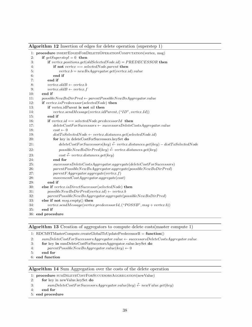
Algorithm 12 Insertion of edges for delete operation (superstep 1)
1: procedure insertEdgesForDeleteOperationComputation(vertex, msg)2: if getSuperstep! = 0 then3: if vertex.positions.get(oldSelectedNode.id) = PREDECESSOR then4: if not vertex == selectedNode.parent then5: vertex.b = newBsAggregator.get(vertex.id).value6: end if7: end if8: vertex.oldB ← vertex.b9: vertex.oldB ← vertex.f
10: end if11: possibleNewBsDirPred← parentPossibleNewBsAggregator.value12: if vertex.isPredecessor(selectedNode) then13: if vertex.idParent is not nil then14: vertex.sendMessage(vertex.idParent, (“ID”, vertex.Id))15: end if16: if vertex.id == selectedNode.predecessorId then17: deleteCostForSuccessors← successorsDeleteCostsAggregator.value18: cost← 019: distToSelectedNode← vertex.distances.get(selectedNode.id)20: for key in deleteCostForSuccessors.keySet do
21: deleteCostForSuccessors(key)+← vertex.distances.get(key)− distToSelectedNode
22: possibleNewBsDirPred(key)+← vertex.distances.get(key)
23: cost+← vertex.distances.get(key)
24: end for25: successorsDeleteCostsAggregator.aggregate(deleteCostForSuccessors)26: parentPossibleNewBsAggregator.aggregate(possibleNewBsDirPred)27: parentFAggregator.aggregate(vertex.f)28: movementCostAggregator.aggregate(cost)29: end if30: else if vertex.isDirectSuccessor(selectedNode) then31: possibleNewBsDirPred(vertex.id)← vertex.b32: parentPossibleNewBsAggregator.aggregate(possibleNewBsDirPred)33: else if not msg.empty() then34: vertex.sendMessage(vertex.predecessorId, (“POSSB”,msg + vertex.b))35: end if36: end procedure
Algorithm 13 Creation of aggregators to compute delete costs(master compute 1)
1: RDCMSTMasterCompute.createGlobalToUpdatePredecessorB = function()
2: sumDeleteCostForSuccessorsAggregator.value← successorsDeleteCostsAggregator.value3: for key in sumDeleteCostForSuccesorsAggregator.value.keySet do4: parentPossibleNewBsAggregator.value(key)← 05: end for6: end function
Algorithm 14 Sum Aggregation over the costs of the delete operation
1: procedure sumDeleteCostForSuccesorsAggregation(newValue)2: for key in newValue.keySet do
3: sumDeleteCostForSuccesorsAggregator.value(key)+← newV alue.get(key)
4: end for5: end procedure
38
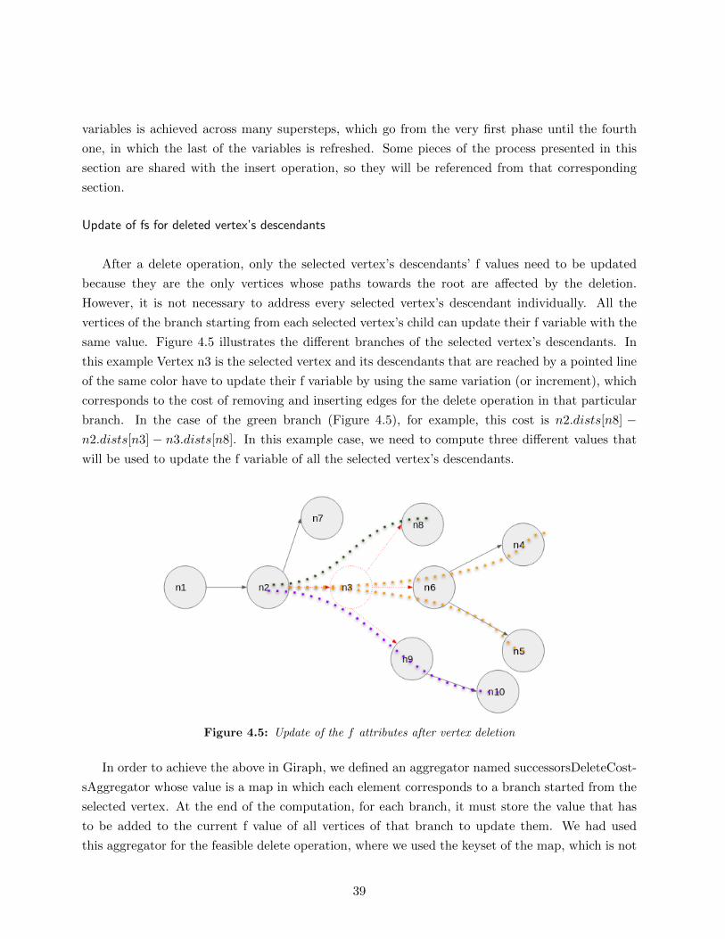
variables is achieved across many supersteps, which go from the very first phase until the fourth
one, in which the last of the variables is refreshed. Some pieces of the process presented in this
section are shared with the insert operation, so they will be referenced from that corresponding
section.
Update of fs for deleted vertex’s descendants
After a delete operation, only the selected vertex’s descendants’ f values need to be updated
because they are the only vertices whose paths towards the root are affected by the deletion.
However, it is not necessary to address every selected vertex’s descendant individually. All the
vertices of the branch starting from each selected vertex’s child can update their f variable with the
same value. Figure 4.5 illustrates the different branches of the selected vertex’s descendants. In
this example Vertex n3 is the selected vertex and its descendants that are reached by a pointed line
of the same color have to update their f variable by using the same variation (or increment), which
corresponds to the cost of removing and inserting edges for the delete operation in that particular
branch. In the case of the green branch (Figure 4.5), for example, this cost is n2.dists[n8] −n2.dists[n3] − n3.dists[n8]. In this example case, we need to compute three different values that
will be used to update the f variable of all the selected vertex’s descendants.
Figure 4.5: Update of the f attributes after vertex deletion
In order to achieve the above in Giraph, we defined an aggregator named successorsDeleteCost-
sAggregator whose value is a map in which each element corresponds to a branch started from the
selected vertex. At the end of the computation, for each branch, it must store the value that has
to be added to the current f value of all vertices of that branch to update them. We had used
this aggregator for the feasible delete operation, where we used the keyset of the map, which is not
39
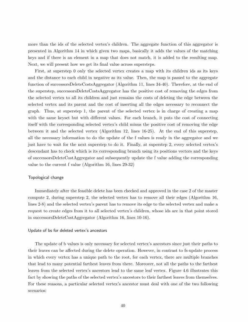
more than the ids of the selected vertex’s children. The aggregate function of this aggregator is
presented in Algorithm 14 in which given two maps, basically it adds the values of the matching
keys and if there is an element in a map that does not match, it is added to the resulting map.
Next, we will present how we get its final value across supersteps.
First, at superstep 0 only the selected vertex creates a map with its children ids as its keys
and the distance to each child in negative as its value. Then, the map is passed to the aggregate
function of successorsDeleteCostsAggregator (Algorithm 11, lines 34-40). Therefore, at the end of
the superstep, successorsDeleteCostsAggregator has the positive cost of removing the edges from
the selected vertex to all its children and just remains the costs of deleting the edge between the
selected vertex and its parent and the cost of inserting all the edges necessary to reconnect the
graph. Thus, at superstep 1, the parent of the selected vertex is in charge of creating a map
with the same keyset but with different values. For each branch, it puts the cost of connecting
itself with the corresponding selected vertex’s child minus the positive cost of removing the edge
between it and the selected vertex (Algorithm 12, lines 16-25). At the end of this superstep,
all the necessary information to do the update of the f values is ready in the aggregator and we
just have to wait for the next superstep to do it. Finally, at superstep 2, every selected vertex’s
descendant has to check which is its corresponding branch using its positions vectors and the keys
of successorsDeleteCostAggregator and subsequently update the f value adding the corresponding
value to the current f value (Algorithm 16, lines 29-32)
Topological change
Immediately after the feasible delete has been checked and approved in the case 2 of the master
compute 2, during superstep 2, the selected vertex has to remove all their edges (Algorithm 16,
lines 2-8) and the selected vertex’s parent has to remove its edge to the selected vertex and make a
request to create edges from it to all selected vertex’s children, whose ids are in that point stored
in successorsDeleteCostAggregator (Algorithm 16, lines 10-16).
Update of bs for deleted vertex’s ancestors
The update of b values is only necessary for selected vertex’s ancestors since just their paths to
their leaves can be affected during the delete operation. However, in contrast to fs-update process
in which every vertex has a unique path to the root, for each vertex, there are multiple branches
that lead to many potential farthest leaves from there. Moreover, not all the paths to the farthest
leaves from the selected vertex’s ancestors lead to the same leaf vertex. Figure 4.6 illustrates this
fact by showing the paths of the selected vertex’s ancestors to their farthest leaves from themselves.
For these reasons, a particular selected vertex’s ancestor must deal with one of the two following
scenarios:
40

Figure 4.6: Update of the b attributes after vertex deletion
1. Its new farthest leaf comes from a branch which was not affected by the delete operation
2. Its new farthest leaf comes from the unique branch that is born from the child that leads to
the path that has been affected by the delete operation. In the same way, the b value of that
child is affected by one of these two scenarios.
Figure 4.7 shows the two scenarios for the vertex n2, which has to decide if its new farthest
leaf comes from the branch of its child n3 or from its other branches. The problem is that it has
to wait for the computation of n3’s b value in order to perform its own. Therefore, we can see the
recursive structure that has to be executed sequentially in order to update b values, starting from
the selected vertex’s parent until the root vertex.
Using the pure computational model of Giraph, these updates will take as many supersteps
as the number of selected vertex’s ancestors. However, using the master compute function and
aggregators features, we follow a different approach. First, across many supersteps, we collect in
some aggregator all the necessary information to do the update, so that in the master compute
function we can compute sequentially each one of the new b values, store them again in a global
variable and use them to update the b values at the next superstep. Next, we will describe this
process in detail.
In order to understand the whole process, we need to keep in mind the two options to update
the b value of a particular selected vertex’s ancestor: The new farthest leave can come from the
branches that are not affected by the delete operation or it can come from the only branch that
is affected by the delete operation. Thus, from the first superstep we start to work in the first of
these scenarios. In lines 41-45 of Algorithm 11, each one of the selected vertex’s ancestors sends its
distance to all of its children. This distance plus the current b value of the child is the distance to
41
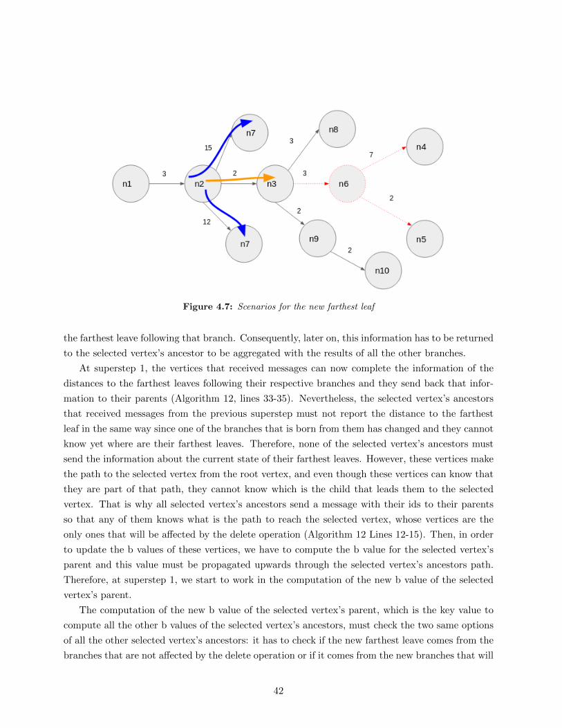
Figure 4.7: Scenarios for the new farthest leaf
the farthest leave following that branch. Consequently, later on, this information has to be returned
to the selected vertex’s ancestor to be aggregated with the results of all the other branches.
At superstep 1, the vertices that received messages can now complete the information of the
distances to the farthest leaves following their respective branches and they send back that infor-
mation to their parents (Algorithm 12, lines 33-35). Nevertheless, the selected vertex’s ancestors
that received messages from the previous superstep must not report the distance to the farthest
leaf in the same way since one of the branches that is born from them has changed and they cannot
know yet where are their farthest leaves. Therefore, none of the selected vertex’s ancestors must
send the information about the current state of their farthest leaves. However, these vertices make
the path to the selected vertex from the root vertex, and even though these vertices can know that
they are part of that path, they cannot know which is the child that leads them to the selected
vertex. That is why all selected vertex’s ancestors send a message with their ids to their parents
so that any of them knows what is the path to reach the selected vertex, whose vertices are the
only ones that will be affected by the delete operation (Algorithm 12 Lines 12-15). Then, in order
to update the b values of these vertices, we have to compute the b value for the selected vertex’s
parent and this value must be propagated upwards through the selected vertex’s ancestors path.
Therefore, at superstep 1, we start to work in the computation of the new b value of the selected
vertex’s parent.
The computation of the new b value of the selected vertex’s parent, which is the key value to
compute all the other b values of the selected vertex’s ancestors, must check the two same options
of all the other selected vertex’s ancestors: it has to check if the new farthest leave comes from the
branches that are not affected by the delete operation or if it comes from the new branches that will
42

be created by connecting the selected vertex’s parent with the selected vertex’s children. We saw
how the distance to the farthest leaf following the last option is computed in section 4.2.3.1 to be
used in the feasible delete operation. It is important to remember that this value is stored, at case
2 of the master compute function, in a global variable named parentBestPossibleNewB (Algorithm
9, line 24).
Now, at superstep 2, we are ready to store all the information required to produce the new
b values of all selected vertex’s ancestors. Thus, this information is going to be stored in the
aggregator AllPredecessorsPossibleNewBsAggregator (Algorithm 9, line 25) whose value is a Map
in which the keys correspond to the id of each one of the selected vertex’s ancestors and the values
to a data structure named ElementsToComputeB whose fields are described next:
• Int idParent: The id of the vertex’s parent
• Dbl possNewB: This is the possible new b value that would come from the farthest leaf of
the branches that were not affected by the delete operation
• Dbl ptlPossNewBs: This is just the distance to the only child that leads to the selected vertex.
This value plus the new b value of that child is the other possible new b value of the vertex.
For the example illustrated in Figure 4.6, the value of AllPredecessorsPossibleNewBsAggregator,
when it is completely aggregated, should look like the structure presented in Listings 4.3
Listing 4.3: AllPredecessorsPossibleNewBsAggregator
{n1 : {
idParent : n i l l
possNewB : 0
ptlPossNewBs : 3
} ,
n2 : {idParent : n1
possNewB : 15
ptlPossNewBs : 2
}}
At superstep 2, whereas selected vertex’s parent can directly update its b value, the other
selected vertex’s ancestors just can store partial information in the ElementsToComputeB Aggre-
gator that just can be completed in the next invocation of the master compute function as far
as sequentially one by one of the new b values of the selected vertex’s ancestors are computed.
Therefore, at this superstep, all selected vertex’s ancestors receive the messages with the possible
43
new b values coming from its unaffected branches, which have to be reduced to a single value that
is the distance to the farthest leaf following those paths. In the case of the selected vertex’s parent,
it just has to compare that value with the parentBestPossibleNewB’s value to update its own b
value (Algorithm 16, lines 17-22). However, the others selected vertex’s ancestors can only put
information into the ElementsToComputeB. They must store the reduced value of the incoming
messages from unaffected branches into the possNewB field. On the other hand, with the message
delivered by its selected vertex’s ancestor child, it can get the value for ptlPossNewBs (Algorithm
16, lines 23-28)
Once all the information of AllPredecessorsPossibleNewBsAggregator is complete, we can com-
pute in the case 3 of the master compute function all the new b values of selected vertex’s ancestors.
Algorithm 17 shows in detail how this is achieved. At the end of the execution of that algorithm,
a new aggregator named newBs will have been created storing a Map with the new b value for
each selected vertex’s ancestor, which is used at superstep 3 to update the corresponding b values
(Algorithm 18, lines 2-6).
Algorithm 15 Compute b value for predecessor of selected vertex (master compute 2 )
1: procedure createGlobalToUpdatePredeccesorsMasterCompute2: parentBestPossibleNewBAggregator.value← max(parentPossibleNewBsAggregator.value)3: end procedure
4.2.4 Insert operation
The insert operation is composed by two sub operations: The best location operation, which is in
charge of computing the place where the selected vertex is going to be inserted; and the update of
the graph’s state produced by the insert operation itself.
4.2.4.1 Best Location Operation
For each vertex there are two possible ways of inserting the selected vertex: 1) directly as a leaf
child of the vertex; and 2) as a parent of the vertex, breaking the existing edge between the vertex
and its old parent. In what follows we use ATLEAF to refer to the first type of location and
ATEDGE to refer to the second one. Figure 4.8 shows both types of location for the vertex n3.
In a nutshell, our strategy to find the best location is the following: for each vertex on the
graph, we compute the cost of inserting the selected vertex in both locations. Then, again for each
vertex, we choose the best “local” location between ATLEAF and ATEDGE (The one with the
lowest cost). Finally, using an aggregator, we choose the best location among all the vertices on
the graph. Next, we will present how the best location operation is performed in Giraph.
At superstep 2, we compute the cost of inserting the selected vertex ATLEAF in each vertex.
This cost just has to be computed if the insertion in that particular location is feasible, that is
44
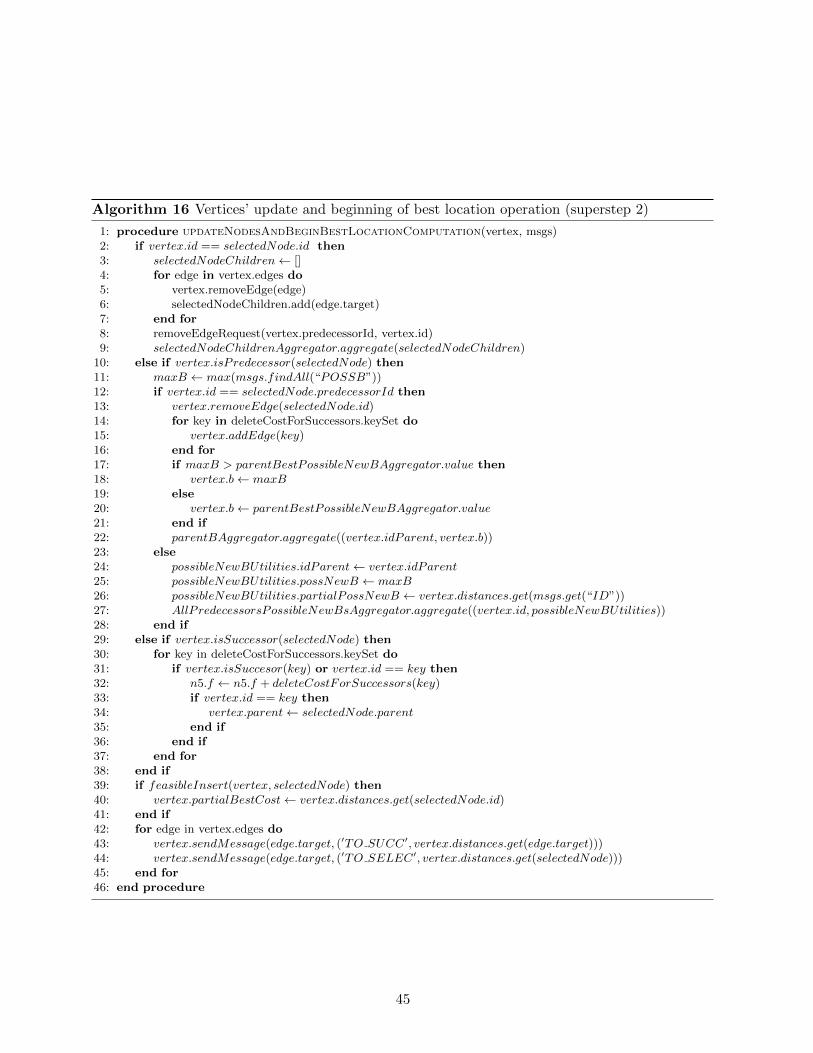
Algorithm 16 Vertices’ update and beginning of best location operation (superstep 2)
1: procedure updateNodesAndBeginBestLocationComputation(vertex, msgs)2: if vertex.id == selectedNode.id then3: selectedNodeChildren← []4: for edge in vertex.edges do5: vertex.removeEdge(edge)6: selectedNodeChildren.add(edge.target)7: end for8: removeEdgeRequest(vertex.predecessorId, vertex.id)9: selectedNodeChildrenAggregator.aggregate(selectedNodeChildren)
10: else if vertex.isPredecessor(selectedNode) then11: maxB ← max(msgs.findAll(“POSSB”))12: if vertex.id == selectedNode.predecessorId then13: vertex.removeEdge(selectedNode.id)14: for key in deleteCostForSuccessors.keySet do15: vertex.addEdge(key)16: end for17: if maxB > parentBestPossibleNewBAggregator.value then18: vertex.b← maxB19: else20: vertex.b← parentBestPossibleNewBAggregator.value21: end if22: parentBAggregator.aggregate((vertex.idParent, vertex.b))23: else24: possibleNewBUtilities.idParent← vertex.idParent25: possibleNewBUtilities.possNewB ← maxB26: possibleNewBUtilities.partialPossNewB ← vertex.distances.get(msgs.get(“ID”))27: AllPredecessorsPossibleNewBsAggregator.aggregate((vertex.id, possibleNewBUtilities))28: end if29: else if vertex.isSuccessor(selectedNode) then30: for key in deleteCostForSuccessors.keySet do31: if vertex.isSuccesor(key) or vertex.id == key then32: n5.f ← n5.f + deleteCostForSuccessors(key)33: if vertex.id == key then34: vertex.parent← selectedNode.parent35: end if36: end if37: end for38: end if39: if feasibleInsert(vertex, selectedNode) then40: vertex.partialBestCost← vertex.distances.get(selectedNode.id)41: end if42: for edge in vertex.edges do43: vertex.sendMessage(edge.target, (′TO SUCC′, vertex.distances.get(edge.target)))44: vertex.sendMessage(edge.target, (′TO SELEC′, vertex.distances.get(selectedNode)))45: end for46: end procedure
45

Algorithm 17 compute b values for selected vertex’s predecessors (master compute 3 )
1: RDCMSTMasterCompute.computeBValues = function()
2: registerAggregator(“bestLocationAggregator”)3: registerAggregator(“newBsAggregator”)4: possibleNewBs← AllPredecessorsPossibleNewBsAggregator.value5: parentId← parentBAggregator.value.id6: bV alue← parentBAggregator.value.b7: while not possibleNewBs.isEmpty() do8: elementToComputeB ← possibleNewBs.get(parentId)9: possNewBFromSelectedNode← elementToComputeB.partialPossibleB + bV alue
10: possNewBFromOtherBranches← elementToComputeB.bFromOtherBranches11: if possNewBFromOtherBranches > possNewBFromSelectedNode then12: bV alue← possNewBFromOtherBranches13: else14: bV alue← possNewBFromSelectedNode15: end if16: newBsAggregator.value(parentId)← bV alue17: formerSuccessorId← parentId18: parentId← elementToComputeB.predecessorId19: possibleNewBs.remove(formerSuccessorId)20: end while21: end function
(a) ATLEAF (b) ATEDGE
Figure 4.8: Example of the two type of location for vertex n3
46
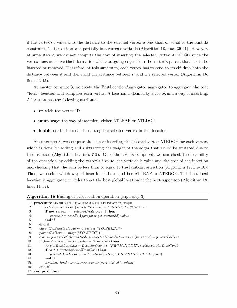
if the vertex’s f value plus the distance to the selected vertex is less than or equal to the lambda
constraint. This cost is stored partially in a vertex’s variable (Algorithm 16, lines 39-41). However,
at superstep 2, we cannot compute the cost of inserting the selected vertex ATEDGE since the
vertex does not have the information of the outgoing edges from the vertex’s parent that has to be
inserted or removed. Therefore, at this superstep, each vertex has to send to its children both the
distance between it and them and the distance between it and the selected vertex (Algorithm 16,
lines 42-45).
At master compute 3, we create the BestLocationAggregator aggregator to aggregate the best
“local” location that computes each vertex. A location is defined by a vertex and a way of inserting.
A location has the following attributes:
• int vId: the vertex ID.
• enum way: the way of insertion, either ATLEAF or ATEDGE
• double cost: the cost of inserting the selected vertex in this location
At superstep 3, we compute the cost of inserting the selected vertex ATEDGE for each vertex,
which is done by adding and subtracting the weight of the edges that would be mutated due to
the insertion (Algorithm 18, lines 7-9). Once the cost is computed, we can check the feasibility
of the operation by adding the vertex’s f value, the vertex’s b value and the cost of the insertion
and checking that the sum be less than or equal to the lambda restriction (Algorithm 18, line 10).
Then, we decide which way of insertion is better, either ATLEAF or ATEDGE. This best local
location is aggregated in order to get the best global location at the next superstep (Algorithm 18,
lines 11-15).
Algorithm 18 Ending of best location operation (superstep 3)
1: procedure finishBestLocationComputation(vertex, msgs)2: if vertex.positions.get(selectedNode.id) = PREDECESSOR then3: if not vertex == selectedNode.parent then4: vertex.b = newBsAggregator.get(vertex.id).value5: end if6: end if7: parentToSelectedNode← msgs.get(“TO SELEC”)8: parentToHere← msgs(“TO SUCC”)9: cost← parentToSelectedNode+ selectedNode.distances.get(vertex.id)− parentToHere
10: if feasibleInsert(vertex, selectedNode, cost) then11: partialBestLocation = Location(vertex, “FROM NODE”, vertex.partialBestCost)12: if cost < vertex.partialBestCost then13: partialBestLocation = Location(vertex, “BREAKING EDGE”, cost)14: end if15: bestLocationAggregator.aggregate(partialBestLocation)16: end if17: end procedure
47
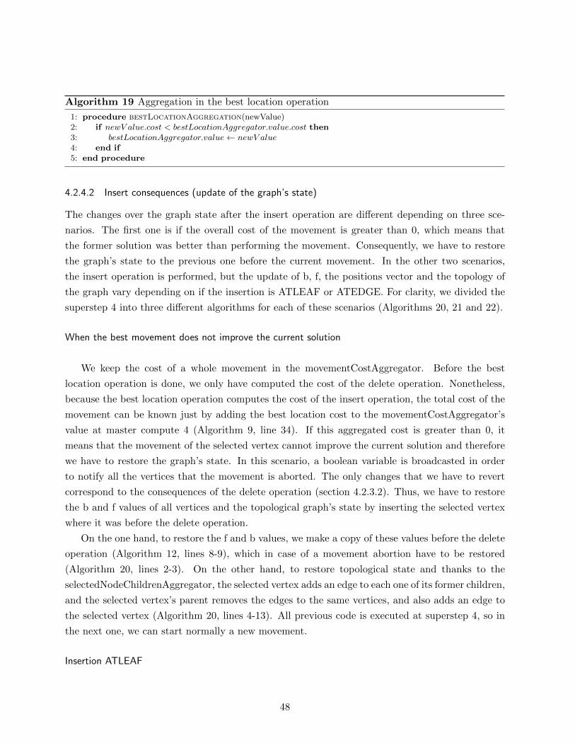
Algorithm 19 Aggregation in the best location operation
1: procedure bestLocationAggregation(newValue)2: if newV alue.cost < bestLocationAggregator.value.cost then3: bestLocationAggregator.value← newV alue4: end if5: end procedure
4.2.4.2 Insert consequences (update of the graph’s state)
The changes over the graph state after the insert operation are different depending on three sce-
narios. The first one is if the overall cost of the movement is greater than 0, which means that
the former solution was better than performing the movement. Consequently, we have to restore
the graph’s state to the previous one before the current movement. In the other two scenarios,
the insert operation is performed, but the update of b, f, the positions vector and the topology of
the graph vary depending on if the insertion is ATLEAF or ATEDGE. For clarity, we divided the
superstep 4 into three different algorithms for each of these scenarios (Algorithms 20, 21 and 22).
When the best movement does not improve the current solution
We keep the cost of a whole movement in the movementCostAggregator. Before the best
location operation is done, we only have computed the cost of the delete operation. Nonetheless,
because the best location operation computes the cost of the insert operation, the total cost of the
movement can be known just by adding the best location cost to the movementCostAggregator’s
value at master compute 4 (Algorithm 9, line 34). If this aggregated cost is greater than 0, it
means that the movement of the selected vertex cannot improve the current solution and therefore
we have to restore the graph’s state. In this scenario, a boolean variable is broadcasted in order
to notify all the vertices that the movement is aborted. The only changes that we have to revert
correspond to the consequences of the delete operation (section 4.2.3.2). Thus, we have to restore
the b and f values of all vertices and the topological graph’s state by inserting the selected vertex
where it was before the delete operation.
On the one hand, to restore the f and b values, we make a copy of these values before the delete
operation (Algorithm 12, lines 8-9), which in case of a movement abortion have to be restored
(Algorithm 20, lines 2-3). On the other hand, to restore topological state and thanks to the
selectedNodeChildrenAggregator, the selected vertex adds an edge to each one of its former children,
and the selected vertex’s parent removes the edges to the same vertices, and also adds an edge to
the selected vertex (Algorithm 20, lines 4-13). All previous code is executed at superstep 4, so in
the next one, we can start normally a new movement.
Insertion ATLEAF
48

Algorithm 20 Restore (superstep 4)
1: procedure restorePreviousMovement(vertex, msg)2: vertex.b← vertex.oldB3: vertex.f ← vertex.oldF4: if vertex == selectedNode then5: for child in selectedNodeChildrenAggregator.value do6: vertex.addEdge(child)7: end for8: else if vertex == selectedV ertex.parent then9: vertex.addEdge(selectedNode)
10: for child in selectedNodeChildrenAggregator.value do11: vertex.removeEdge(child)12: end for13: end if14: end procedure
The insertion ATLEAF is the simplest way of insertion so it is the one that implies fewer changes
in the state of the graph. First of all, the topological change simply is made by inserting an edge
between the best location vertex and the selected vertex (Algorithm 21, line 22).
Then, it is noticeable that we do not have to update the f value of any vertex in the graph
except the selected vertex itself. This is due to none of the paths from the vertices to the root are
affected. Therefore, the best location vertex just has to send its own f value plus the distance to
the selected vertex (Algorithm 21, lines 23-24) in order for the selected vertex be able to replace
its f value with the message’s value in the next superstep (Algorithm 11, line 9).
Moreover, even though the update of the b values is very similar as in the delete operation,
none of the current paths to the leaves are affected by the operation. As a result, every ancestor
just has to check if the distance to the selected vertex is greater than its actual b value. However,
although this seems to be an easier procedure, it has to use practically the same algorithm that
we present in section 4.2.3.2. So, at superstep 4, it starts by updating the b value of the selected
vertex’s parent. At the same time, the ancestors of the best location vertex send their ids to their
parents in order to unfold the path towards the new leaf (Algorithm 21, line 25). From the next
superstep (Superstep 0), the update is performed in the same way the delete operation does it.
The only difference is that for each ancestor, its corresponding elementsToComputeB.possNwBs is
equal to its current b value (because none of the paths to the leaves are affected by the operation).
Therefore, at master compute 1 (Algorithm 9, line 12) all the new b values are computed and by
superstep 1, all the ancestors have updated their b values (Algorithm 12, lines 4-6).
Finally, we have to deal with a variable that we have not modified until now. After the insert
operation, the positions of all the vertices about the selected vertex have changed as well as the
positions of the selected vertex about all the other vertices. Therefore, all the new ancestors of the
selected vertex (the best location vertex and all its ancestors) have to update their positions about
the selected vertex with the label ANCESTOR (Algorithm 21, lines 8 and 21), whereas all the other
vertices in the graph have to do the same but with the label NONE (Algorithm 21, lines 13 and
49

28). On the other hand, all the vertices in the graph send a message to the selected vertex with
the position that it needs to update in its own positions array in the next superstep. The selected
vertex’s ancestors send the DESCENDANT label and the vertices that are neither ancestors nor
descendants send the NONE label. Each of these messages is sent in a tuple with the id of the
emisor vertex and the label, which are used at superstep 0 to update the selected vertex’s positions
array (Algorithm 11, lines 4-8)
Algorithm 21 Nodes’ update and insert operation ATLEAF (superstep 4)
1: procedure insertOperationAndUpdateNodesComputation(vertex, msg)2: if vertex == selectedNode then3: if bestLocation.way == “FROM NODE” then4: vertex.parent← bestLocation.node5: end if6: end if7: if vertex.isPredecessor(bestLocation.node) then8: vertex.positions.get(selectedNode.id) = PREDECESSOR9: sendMessage(vertex.parent, (“ID”, vertex.id))
10: sendMessage(selectedNode, (vertex.id, PREDECESSOR))11: else if vertex.isSuccessor(bestLocation.node) then12: if bestLocation.way == “FROM NODE” then13: vertex.positions(selectedNode) = NONE14: sendMessage(selectedNode, (vertex.id,NONE))15: end if16: else if vertex == bestLocation.node then17: if bestLocation.way == “FROM NODE” then18: if bestLocation.cost > vertex.b then19: vertex.b← bestLocation.cost20: end if21: vertex.positions.get(selectedNode.id) = PREDECESSOR22: vertex.addEdge(selectedNode.id)23: selectedNodeF ← vertex.f + vertex.distances.get(selectedNode.id)24: sendMessage(selectedNode, (“F”, selectedNodeF ))25: sendMessage(vertex.parent, (“ID”, vertex.id))26: end if27: else28: vertex.positions.get(selectedNode) = NONE29: sendMessage(vertex.parent, (“PAR B”, vertex.b))30: end if31: end procedure
Insertion ATEDGE
The insertion ATEDGE is a little more complex because it affects more vertices in the graph.
Firstly, the topological changes are made by both the selected vertex and the best location vertex’s
parent (Algorithm 22, lines 5, 15 and 16).
All the new selected vertex’s descendants have to update their f value by adding the best location
cost to their current f values (Algorithm 22, lines 24 and 29). These vertices are the best location
vertex and all its descendants. Additionally, the selected vertex’s f value has to be updated in
50

exactly the same way as in the insertion ATLEAF.
The insertion ATEDGE affects the distance from the new selected vertex’s ancestor to some of
the leaves. Therefore, we can use the concept of affected and unaffected branches (section 4.2.3.2)
in order to update their b values. Thus, the idea is for each new selected vertex’s ancestor to check
whether the new farthest leaf comes from the unaffected branches or from the affected one. In
order to compute the farthest leaf coming from the unaffected branches, the vertices, which are
neither ancestors nor descendants of the best location vertex, send their b values to their parents
(Algorithm 22, line 37). At the next superstep, the new descendants of the selected vertex can
compute the distance to the farthest leaves following its unaffected branches just by adding the
distance to the emisor vertex to the value of the message itself. Then, the maximum of these values
has to be chosen and stored in elementsToComputeB.possNwBs (Algorithm 11, line 28). On the
other hand, unlike the delete operation, there is only one branch from the new selected vertex’s
parent that is affected by the insert operation. Consequently, we just have to compare the distance
to the farthest leaf following this branch with the one computed from the unaffected branches.
In order to compute this distance, we use an aggregator named parentBestPossibleNewB, whose
aggregate function just sum up double values. Therefore, we have to add up the best location
vertex’s b value and the distance from the new selected vertex’ parent to the the best location
vertex crossing the new two edges (Algorithm 22, lines 6, 17 and 32). Once the the new b value
of the selected vertex’s parent has been updated (Algorithm 11, lines 18-24), the procedure to
update the b values of all the selected vertex’s ancestors is the same as the delete operation and
the insert operation ATLEAF. Finally to update the selected vertex’s b value, at superstep 4, the
best location vertex sends to it its own b value (Algorithm 22, line 33), which has to be used in
the next superstep by the selected vertex to make the update (Algorithm 11, line 18).
Lastly, the update of the positions array is pretty similar to the insertion ATLEAF, except that
the new selected vertex’s descendants also have to update their positions about the selected vertex,
and send a message to it in order to allow the update of its own array.
51

Algorithm 22 Nodes’ update and insert operation ATEDGE(superstep 4)
1: procedure insertOperationAndUpdateNodesComputation(vertex, msg)2: if vertex == selectedNode then3: if bestLocation.way == “BREAKING EDGE” then4: vertex.parent = bestLocation.node.parent5: vertex.addEdge(bestLocation.node)6: parentBestPossibleNewBAggregator.aggregate(vertex.distances.get(bestLocation.id))7: end if8: end if9: if vertex.isPredecessor(bestLocation.node) then
10: vertex.positions.get(selectedNode.id) = PREDECESSOR11: sendMessage(vertex.parent, (“ID”, vertex.id))12: sendMessage(selectedNode, (vertex.id, PREDECESSOR))13: if vertex == bestLocation.node.parent then14: if bestLocation.way == “BREAKING EDGE” then15: vertex.addEdge(selectedNode.id)16: vertex.removeEdge(bestLocation.node.id)17: parentBestPossibleNewBAggregator.aggregate(vertex.distances.get(selectedNode.id))18: selectedNodeF ← vertex.f + vertex.distances.get(selectedNode.id)19: sendMessage(selectedNode, (“F”, selectedNodeF ))20: end if21: end if22: else if vertex.isSuccessor(bestLocation.node) then23: if bestLocation.way == “BREAKING EDGE” then24: vertex.f ← vertex.f + bestLocation.cost25: vertex.positions.get(selectedNode) = SUCCESSOR26: end if27: else if vertex == bestLocation.node then28: if bestLocation.way == “BREAKING EDGE” then29: vertex.f ← vertex.f + bestLocation.cost30: vertex.positions.get(selectedNode) = SUCCESSOR31: vertex.parent = selectedNode32: parentBestPossibleNewBAggregator.aggregate(vertex.b)33: sendMessage(selectedNode, (“BEST LOCATION B”, vertex.b))34: end if35: else36: vertex.positions.get(selectedNode) = NONE37: sendMessage(vertex.parent, (“PAR B”, vertex.b))38: end if39: end procedure
52
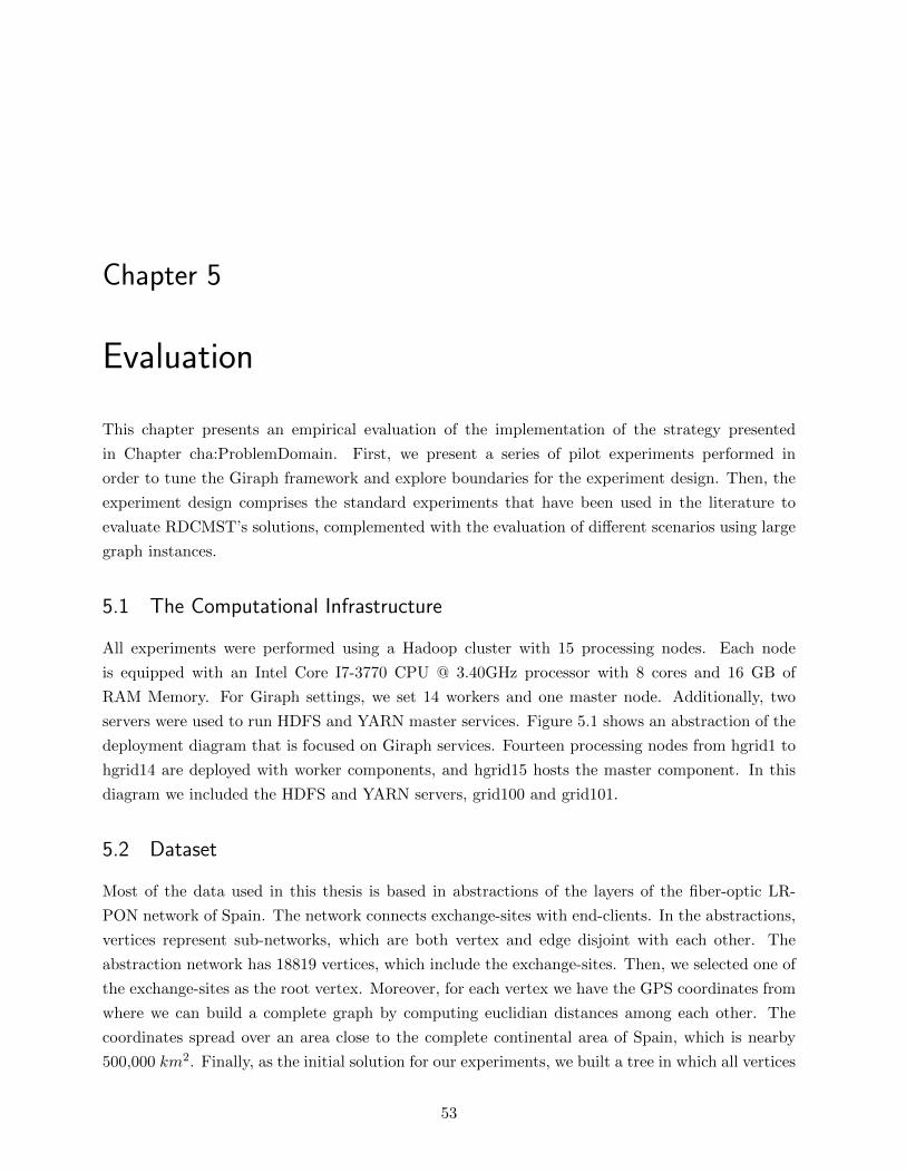
Chapter 5
Evaluation
This chapter presents an empirical evaluation of the implementation of the strategy presented
in Chapter cha:ProblemDomain. First, we present a series of pilot experiments performed in
order to tune the Giraph framework and explore boundaries for the experiment design. Then, the
experiment design comprises the standard experiments that have been used in the literature to
evaluate RDCMST’s solutions, complemented with the evaluation of different scenarios using large
graph instances.
5.1 The Computational Infrastructure
All experiments were performed using a Hadoop cluster with 15 processing nodes. Each node
is equipped with an Intel Core I7-3770 CPU @ 3.40GHz processor with 8 cores and 16 GB of
RAM Memory. For Giraph settings, we set 14 workers and one master node. Additionally, two
servers were used to run HDFS and YARN master services. Figure 5.1 shows an abstraction of the
deployment diagram that is focused on Giraph services. Fourteen processing nodes from hgrid1 to
hgrid14 are deployed with worker components, and hgrid15 hosts the master component. In this
diagram we included the HDFS and YARN servers, grid100 and grid101.
5.2 Dataset
Most of the data used in this thesis is based in abstractions of the layers of the fiber-optic LR-
PON network of Spain. The network connects exchange-sites with end-clients. In the abstractions,
vertices represent sub-networks, which are both vertex and edge disjoint with each other. The
abstraction network has 18819 vertices, which include the exchange-sites. Then, we selected one of
the exchange-sites as the root vertex. Moreover, for each vertex we have the GPS coordinates from
where we can build a complete graph by computing euclidian distances among each other. The
coordinates spread over an area close to the complete continental area of Spain, which is nearby
500,000 km2. Finally, as the initial solution for our experiments, we built a tree in which all vertices
53
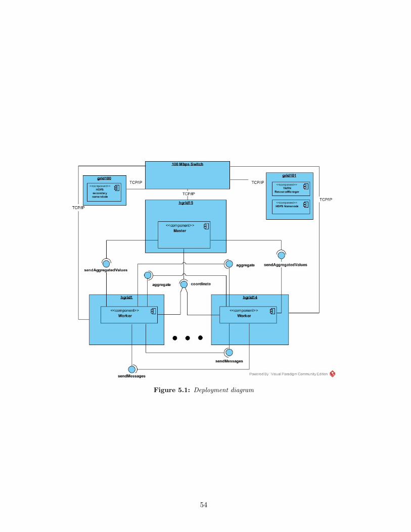
Figure 5.1: Deployment diagram
54
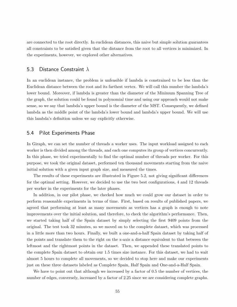
are connected to the root directly. In euclidean distances, this naive but simple solution guarantees
all constraints to be satisfied given that the distance from the root to all vertices is minimized. In
the experiments, however, we explored other alternatives.
5.3 Distance Constraint λ
In an euclidean instance, the problem is unfeasible if lambda is constrained to be less than the
Euclidean distance between the root and its farthest vertex. We will call this number the lambda’s
lower bound. Moreover, if lambda is greater than the diameter of the Minimum Spanning Tree of
the graph, the solution could be found in polynomial time and using our approach would not make
sense, so we say that lambda’s upper bound is the diameter of the MST. Consequently, we defined
lambda as the middle point of the lambda’s lower bound and lambda’s upper bound. We will use
this lambda’s definition unless we say explicitly otherwise.
5.4 Pilot Experiments Phase
In Giraph, we can set the number of threads a worker uses. The input workload assigned to each
worker is then divided among the threads, and each one computes its group of vertices concurrently.
In this phase, we tried experimentally to find the optimal number of threads per worker. For this
purpose, we took the original dataset, performed ten thousand movements starting from the naive
initial solution with a given input graph size, and measured the times.
The results of these experiments are illustrated in Figure 5.2, not giving significant differences
for the optimal setting. However, we decided to use the two best configurations, 4 and 12 threads
per worker in the experiments for the later phases.
In addition, in our pilot phase, we checked how much we could grow our dataset in order to
perform reasonable experiments in terms of time. First, based on results of published papers, we
agreed that performing at least as many movements as vertices has a graph is enough to note
improvements over the initial solution, and therefore, to check the algorithm’s performance. Then,
we started taking half of the Spain dataset by simply selecting the first 9409 points from the
original. The test took 32 minutes, so we moved on to the complete dataset, which was processed
in a little more than two hours. Finally, we built a one-and-a-half Spain dataset by taking half of
the points and translate them to the right on the x-axis a distance equivalent to that between the
leftmost and the rightmost points in the dataset. Then, we appended these translated points to
the complete Spain dataset to obtain our 1.5 times size instance. For this dataset, we had to wait
almost 5 hours to complete all movements, so we decided to stop here and make our experiments
just on these three datasets labeled as Complete Spain, Half Spain and One-and-a-Half Spain.
We have to point out that although we increased by a factor of 0.5 the number of vertices, the
number of edges, conversely, increased by a factor of 2.25 since we are considering complete graphs.
55
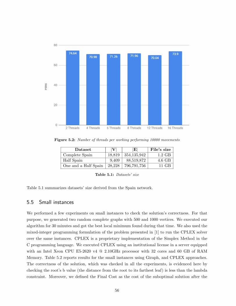
Figure 5.2: Number of threads per working performing 10000 movements
Dataset |V| |E| File’s size
Complete Spain 18,819 354,135,942 1.2 GB
Half Spain 9,409 88,519,872 4.6 GB
One and a Half Spain 28,228 796,791,756 11 GB
Table 5.1: Datasets’ size
Table 5.1 summarizes datasets’ size derived from the Spain network.
5.5 Small instances
We performed a few experiments on small instances to check the solution’s correctness. For that
purpose, we generated two random complete graphs with 500 and 1000 vertices. We executed our
algorithm for 30 minutes and got the best local minimum found during that time. We also used the
mixed-integer programming formulation of the problem presented in [1] to run the CPLEX solver
over the same instances. CPLEX is a proprietary implementation of the Simplex Method in the
C programming language. We executed CPLEX using an institutional license in a server equipped
with an Intel Xeon CPU E5-2620 v4 @ 2.10GHz processor with 32 cores and 60 GB of RAM
Memory. Table 5.2 reports results for the small instances using Giraph, and CPLEX approaches.
The correctness of the solution, which was checked in all the experiments, is evidenced here by
checking the root’s b value (the distance from the root to its farthest leaf) is less than the lambda
constraint. Moreover, we defined the Final Cost as the cost of the suboptimal solution after the
56
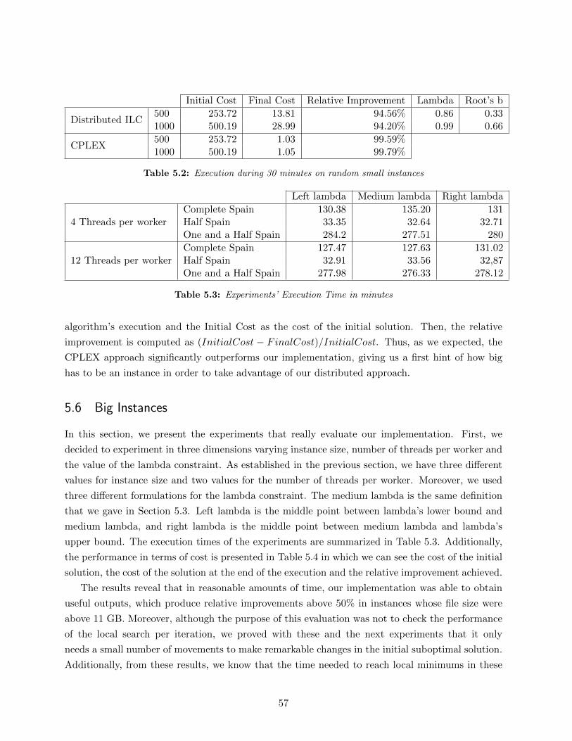
Initial Cost Final Cost Relative Improvement Lambda Root’s b
Distributed ILC500 253.72 13.81 94.56% 0.86 0.331000 500.19 28.99 94.20% 0.99 0.66
CPLEX500 253.72 1.03 99.59%1000 500.19 1.05 99.79%
Table 5.2: Execution during 30 minutes on random small instances
Left lambda Medium lambda Right lambda
4 Threads per workerComplete Spain 130.38 135.20 131Half Spain 33.35 32.64 32.71One and a Half Spain 284.2 277.51 280
12 Threads per workerComplete Spain 127.47 127.63 131.02Half Spain 32.91 33.56 32,87One and a Half Spain 277.98 276.33 278.12
Table 5.3: Experiments’ Execution Time in minutes
algorithm’s execution and the Initial Cost as the cost of the initial solution. Then, the relative
improvement is computed as (InitialCost − FinalCost)/InitialCost. Thus, as we expected, the
CPLEX approach significantly outperforms our implementation, giving us a first hint of how big
has to be an instance in order to take advantage of our distributed approach.
5.6 Big Instances
In this section, we present the experiments that really evaluate our implementation. First, we
decided to experiment in three dimensions varying instance size, number of threads per worker and
the value of the lambda constraint. As established in the previous section, we have three different
values for instance size and two values for the number of threads per worker. Moreover, we used
three different formulations for the lambda constraint. The medium lambda is the same definition
that we gave in Section 5.3. Left lambda is the middle point between lambda’s lower bound and
medium lambda, and right lambda is the middle point between medium lambda and lambda’s
upper bound. The execution times of the experiments are summarized in Table 5.3. Additionally,
the performance in terms of cost is presented in Table 5.4 in which we can see the cost of the initial
solution, the cost of the solution at the end of the execution and the relative improvement achieved.
The results reveal that in reasonable amounts of time, our implementation was able to obtain
useful outputs, which produce relative improvements above 50% in instances whose file size were
above 11 GB. Moreover, although the purpose of this evaluation was not to check the performance
of the local search per iteration, we proved with these and the next experiments that it only
needs a small number of movements to make remarkable changes in the initial suboptimal solution.
Additionally, from these results, we know that the time needed to reach local minimums in these
57
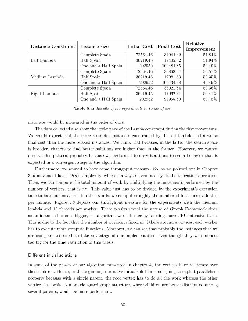
Distance Constraint Instance size Initial Cost Final CostRelativeImprovement
Left LambdaComplete Spain 72564.46 34944.42 51.84%Half Spain 36219.45 17405.82 51.94%One and a Half Spain 202952 100484.85 50.49%
Medium LambdaComplete Spain 72564.46 35868.64 50.57%Half Spain 36219.45 17981.83 50.35%One and a Half Spain 202952 100434.38 49.49%
Right LambdaComplete Spain 72564.46 36021.84 50.36%Half Spain 36219.45 17962.31 50.41%One and a Half Spain 202952 99955.80 50.75%
Table 5.4: Results of the experiments in terms of cost
instances would be measured in the order of days.
The data collected also show the irrelevance of the Lamba constraint during the first movements.
We would expect that the more restricted instances constrained by the left lambda had a worse
final cost than the more relaxed instances. We think that because, in the latter, the search space
is broader, chances to find better solutions are higher than in the former. However, we cannot
observe this pattern, probably because we performed too few iterations to see a behavior that is
expected in a convergent stage of the algorithm.
Furthermore, we wanted to have some throughput measure. So, as we pointed out in Chapter
3, a movement has a O(n) complexity, which is always determined by the best location operation.
Then, we can compute the total amount of work by multiplying the movements performed by the
number of vertices, that is n2. This value just has to be divided by the experiment’s execution
time to have our measure. In other words, we compute roughly the number of locations evaluated
per minute. Figure 5.3 depicts our throughput measure for the experiments with the medium
lambda and 12 threads per worker. These results reveal the nature of Giraph Framework since
as an instance becomes bigger, the algorithm works better by tackling more CPU-intensive tasks.
This is due to the fact that the number of workers is fixed, so if there are more vertices, each worker
has to execute more compute functions. Moreover, we can see that probably the instances that we
are using are too small to take advantage of our implementation, even though they were almost
too big for the time restriction of this thesis.
Different initial solutions
In some of the phases of our algorithm presented in chapter 4, the vertices have to iterate over
their children. Hence, in the beginning, our naive initial solution is not going to exploit parallelism
properly because with a single parent, the root vertex has to do all the work whereas the other
vertices just wait. A more elongated graph structure, where children are better distributed among
several parents, would be more performant.
58
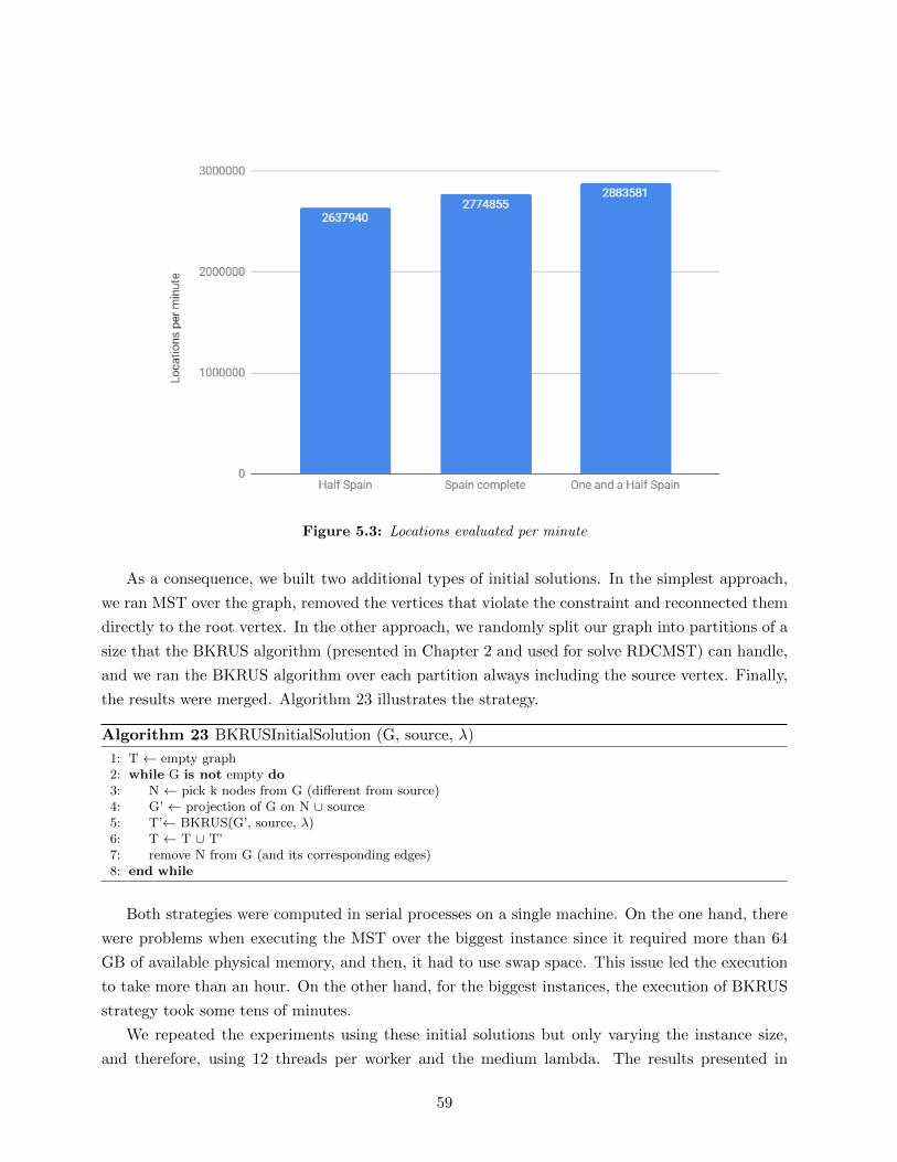
Figure 5.3: Locations evaluated per minute
As a consequence, we built two additional types of initial solutions. In the simplest approach,
we ran MST over the graph, removed the vertices that violate the constraint and reconnected them
directly to the root vertex. In the other approach, we randomly split our graph into partitions of a
size that the BKRUS algorithm (presented in Chapter 2 and used for solve RDCMST) can handle,
and we ran the BKRUS algorithm over each partition always including the source vertex. Finally,
the results were merged. Algorithm 23 illustrates the strategy.
Algorithm 23 BKRUSInitialSolution (G, source, λ)
1: T ← empty graph2: while G is not empty do3: N ← pick k nodes from G (different from source)4: G’ ← projection of G on N ∪ source5: T’← BKRUS(G’, source, λ)6: T ← T ∪ T’7: remove N from G (and its corresponding edges)8: end while
Both strategies were computed in serial processes on a single machine. On the one hand, there
were problems when executing the MST over the biggest instance since it required more than 64
GB of available physical memory, and then, it had to use swap space. This issue led the execution
to take more than an hour. On the other hand, for the biggest instances, the execution of BKRUS
strategy took some tens of minutes.
We repeated the experiments using these initial solutions but only varying the instance size,
and therefore, using 12 threads per worker and the medium lambda. The results presented in
59
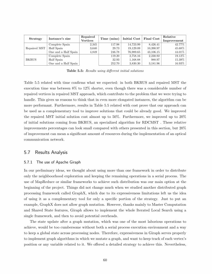
Strategy Instance’s sizeRepairedVertices
Time (mins) Initial Cost Final CostRelativeImprovement
Repaired MSTComplete Spain 2,345 117.98 14,723.99 8,426.41 42.77%Half Spain 3,640 29.73 19,129.09 10,390.97 45.68%One and a Half Spain 4,849 246.78 76,989.65 43,106.15 44.01%
BKRUSComplete Spain 119.20 2,758.16 2,230.92 19.12%Half Spain 32.93 1,168.88 988.97 15.39%One and a Half Spain 252.70 3,830.30 3,181.96 16.93%
Table 5.5: Results using different initial solutions
Table 5.5 related with time confirms what we expected: in both BKRUS and repaired MST the
execution time was between 8% to 12% shorter, even though there was a considerable number of
repaired vertices in repaired MST approach, which contribute to the problem that we were trying to
handle. This gives us reasons to think that in even more elongated instances, the algorithm can be
more performant. Furthermore, results in Table 5.5 related with cost prove that our approach can
be used as a complementary tool to improve solutions that could be already good. We improved
the repaired MST initial solution cost almost up to 50%. Furthermore, we improved up to 20%
of initial solutions coming from BKRUS, an specialized algorithm for RDCMST . These relative
improvements percentages can look small compared with others presented in this section, but 20%
of improvement can mean a significant amount of resources during the implementation of an optical
communication network.
5.7 Results Analysis
5.7.1 The use of Apache Giraph
In our preliminary ideas, we thought about using more than one framework in order to distribute
only the neighboorhood exploration and keeping the remaining operations in a serial process. The
use of MapReduce or similar frameworks to achieve such distribution was our main option at the
beginning of the project. Things did not change much when we studied another distributed graph
processing framework called GraphX, which due to its expressiveness limitations left us the idea
of using it as a complementary tool for only a specific portion of the strategy. Just to put an
example, GraphX does not allow graph mutation. However, thanks mainly to Master Computation
and Shared State features, Giraph allows to implement the whole Iterated Local Search using a
single framework, and then to avoid potential overheads.
The state update after a graph mutation, which was one of the most laborious operations to
achieve, would be too cumbersome without both a serial process execution environment and a way
to keep a global state across processing nodes. Therefore, expressiveness in Giraph serves properly
to implement graph algorithms in which we mutate a graph, and want to keep track of each vertex’s
position or any variable related to it. We offered a detailed strategy to achieve this. Nevertheless,
60
Giraph API can still be improved to solve this kind of problems.
The only way to implement shared state in Giraph is by the aggregator’s philosophy, in which
we have to use a commutative and associative function in order to store data. However, it is not
always desirable to aggregate our global variables. For example, with the aggregator parentPossi-
bleNewBsAggregator (Algorithm 14), we wanted to store a hashmap that allows its extension and
updating its elements. Storing such a structure using an aggregator comes with performance penal-
ties since for each aggregate function invocation, we have to get through the entire structure, and
it is invoked several times. To extend Giraph with a specialized distributed data structure without
the limitations of the aggregators would help to build a better implementation of our strategy.
To finish this Giraph analysis, we want to highlight the flexible granularity that we could achieve
in this framework thanks to the vertex-centric programming paradigm. The grain size is determined
by the number of vertices a worker has assigned. To be precise, the total amount of work of each
worker before communication is the execution of all vertices’ compute function. Therefore, thanks
to the graph partition performed by Giraph, we can say that our solution allows an automatic
uniform-balance distribution regardless of the number of processing nodes.
5.7.2 An Implementation for Big Data
We evaluated our distributed strategy in different scenarios, which included random no-euclidean
instances, a real LP-RON network instance and variations of it in order to establish the boundaries
of this project. The implementation allows us to work with instances that outgrow the memory
capacity of a single machine, making remarkable improvements over solutions that even come from
outputs of other strategies. Thus, it certainly can be used in RDCMST problem as a primary or
complementary tool. Moreover, our results seem to show that our implementation’s performance
improves as the instance grows, which is promissory since in this thesis we are working with an
abstraction network that is smaller than the real one.
Furthermore, Giraph is built on top of the highly scalable system Hadoop, in which just by
adding more processing nodes to the cluster, we can easily increase both processing power and
memory capacity. For time reasons, we did not perform experiments varying the number of node
processors, which would give us valuable information about the scalability of our implementation.
However, there is no reason to think that this is not able to handle much bigger instances. Finally,
we would have liked to evaluate the strategy using more real instances of networks with different
configurations and to look for the optimum number of workers that deal with the dataset used.
However, obtaining such datasets is really difficult. We hope to tackle these issues in future work.
5.7.3 Final remarks
In the end, this thesis pursued two main goals, one derived from the other. First, we looked for
a distributed approach to solve RDCMST, and as a consequence, we ran into the Apache Giraph
61
framework. Then, we decided to evaluate how fast, simple, and scalable is Giraph to implement
solutions to problems like RDCMST.
We discovered the Local Search, stated in Algorithm 8, can be implemented entirely using
Giraph. Moreover, most of the logic, including the key parts of the search, was implemented easily
with the core of the vertex-centric programming paradigm. Nevertheless, some details, related to
preserving state, needed more advanced features of Giraph, which involved extra difficulties in the
algorithm’s design.
Conclusively, in this thesis, we confirmed that scaling the input size for the RDCMST problem
had no impact on us as developers, and the code executions show acceptable results in instances
that could be not large enough to exploit Giraph’s potential.
62
Chapter 6
Conclusions and Future Work
In this thesis, we presented the first known distributed strategy to solve the RDCMST problem,
which was based on the idea of a parallel neighborhood exploration. The implementation of the
strategy on a distributed software architecture allows us to deal with problem instances of ten of
thousands of vertices, which is a size that has not been reported until now.
We designed, implemented and presented a collection of algorithms that serve to solve common
problems in the design of graph algorithms using the vertex-centric programming paradigm and,
consequently, a distributed architecture. Our algorithms can be used in procedures in which there
can be mutations in directed graphs, and we want to keep track of each vertex’s position or any
variable related to it. The design of these algorithms was the hardest work in this project, and we
hope them to be a valuable contribution.
The vertex-centric programming paradigm gave us a flexible task granularity for distributing
the problem solution, based on the fact that every vertex has to compute its micro local search op-
erations. Moreover, the open-source framework Apache Giraph offered us a distributed architecture
on where to run our algorithm by exploiting computational resources. However, although Giraph
allowed us to solve big instances of the problem, it penalizes the execution on small instances that
have tested previous approaches.
The results of this thesis suggest the potential of the implementation to handle bigger problem
instances than those we evaluated. However, they also show the performance weakness of our
solution to solve the problem instances that have been validated in the literature, which are too
small to take advantage of our distributed approach. However, this limitation is found in almost
every other solution implemented in this kind of distributed frameworks. Therefore, these results
are focused on how well we can solve big instances instead of comparing the performance of our
approach with previous approaches, even though we checked that our implementation produced
correct solutions.
Moreover, we show that our performance results are being affected by the structure of the naive
initial solution we proposed. The huge vertex degree of the root in such structure reduces the
63
parallel level that the algorithm can achieve in its initial iterations. We followed two strategies to
get more elongated initial solutions and, besides the performance improvements, we confirm that
our implementations could be used as a complementary tool to refine already good solutions.
Beyond that, despite we were able to deal with problem instances of ten of thousands of vertices,
we could not establish with certainty the real boundaries of our solution. The time restrictions of
this project made it impossible to experiment with bigger instances in order to check performance
in such executions. Nonetheless, our contribution weights beyond our implementation since the pro-
posed strategy can be coded and deployed in other architectures that may include shared-memory
approaches or even alternative distributed frameworks that use the vertex-centric programming
model [8]. Different implementations could offer better or worse performance depending on the
problem instances.
Getting a distributed solution of RDCMST left us very close to obtaining a distributed solu-
tion for EDRDCMT, whose sequential solution’s algorithm inspired our approach. Likewise, our
approach could help to solve generalizations or derivations of RDCMST.
As future work, we want to evaluate our implementation more thoroughly, by taking account
its scalability, and with that, exploring the real boundaries of it. To achieve this goal, we would like
to use the original LR-PON networks of some European countries. Also, we would like to explore
some additional Giraph’s features such as custom graph partition, in order to improve performance.
Finally, we want to implement our strategy using other distributed software architectures and
measure performance differences regarding problem size so we can make a complete analysis of the
pros and cons of the different implementations.
64

Appendix A
Movement illustration
Figure A.1 illustrates the whole strategy introduced in Chapter 4, which is a description of a
complete movement including all its different scenarios. Next, we explain how this illustration
must be read.
To begin with, there are two kinds of stages within a movement and both have different exe-
cution environments. Then, for each phase two classes of images are shown, one for the superstep
computation stage that is executed in parallel by the workers and the other one for the master
computation stage which is executed sequentially by the master node. Nevertheless, the superstep
computation stage often requires several images per phase whereas the master computation stage
always requires a single image.
The master computation stage only deals with the state of the global variables: the broadcasted
variables, reducers and aggregators, which in these illustrations are treated without differentiation.
These global variables are represented as rectangles with squared corners drawn in black, in whose
background is illustrated their current state. When that background is colored with green, it means
the variable is being initialized, which can only happen in the master computation stage. Moreover,
a variable’s initialization always includes its type besides its initial value.
Conversely, in the superstep computation stages, some vertices are circled by colors. For one
vertex, this means that its compute function is executed and sometimes also a rounded corner
rectangle is drawn with the same color in order to contain the most significant pseudocode of the
function. Furthermore, when the vertex’s compute function is writing a global variable, the changes
produced by it are painted with the same color within the variable’s rectangle. For instance, vertex
n6 is writing the movement cost at superstep 0 in Figure A.1b. In addition, images show outgoing
messages as envelopes with their content written next to them.
Finally, a big rounded corner rectangle drawn with black, which is always put in the top right
corner of supersteps computations, shows the pseudocode that defines how the different colors are
assigned to each vertex in the graph.
These images were made as a complementary tool to understand what is written in this chapter
65

and therefore they are a graphic illustration of the algorithms presented here. As a consequence,
they are not supposed to be understood only by themselves.
66
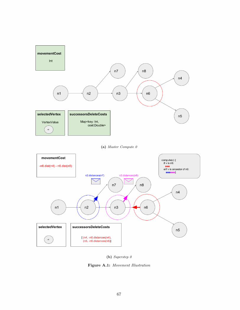
(a) Master Compute 0
(b) Superstep 0
Figure A.1: Movement Illustration
67
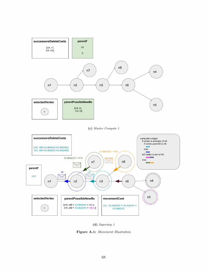
(c) Master Compute 1
(d) Superstep 1
Figure A.1: Movement Illustration
68
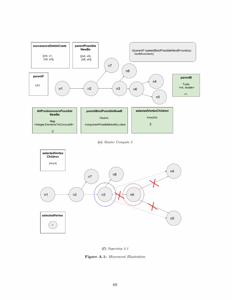
(e) Master Compute 2
(f) Superstep 2-1
Figure A.1: Movement Illustration
69

(g) Superstep 2-2
(h) Superstep 2-3
Figure A.1: Movement Illustration
70
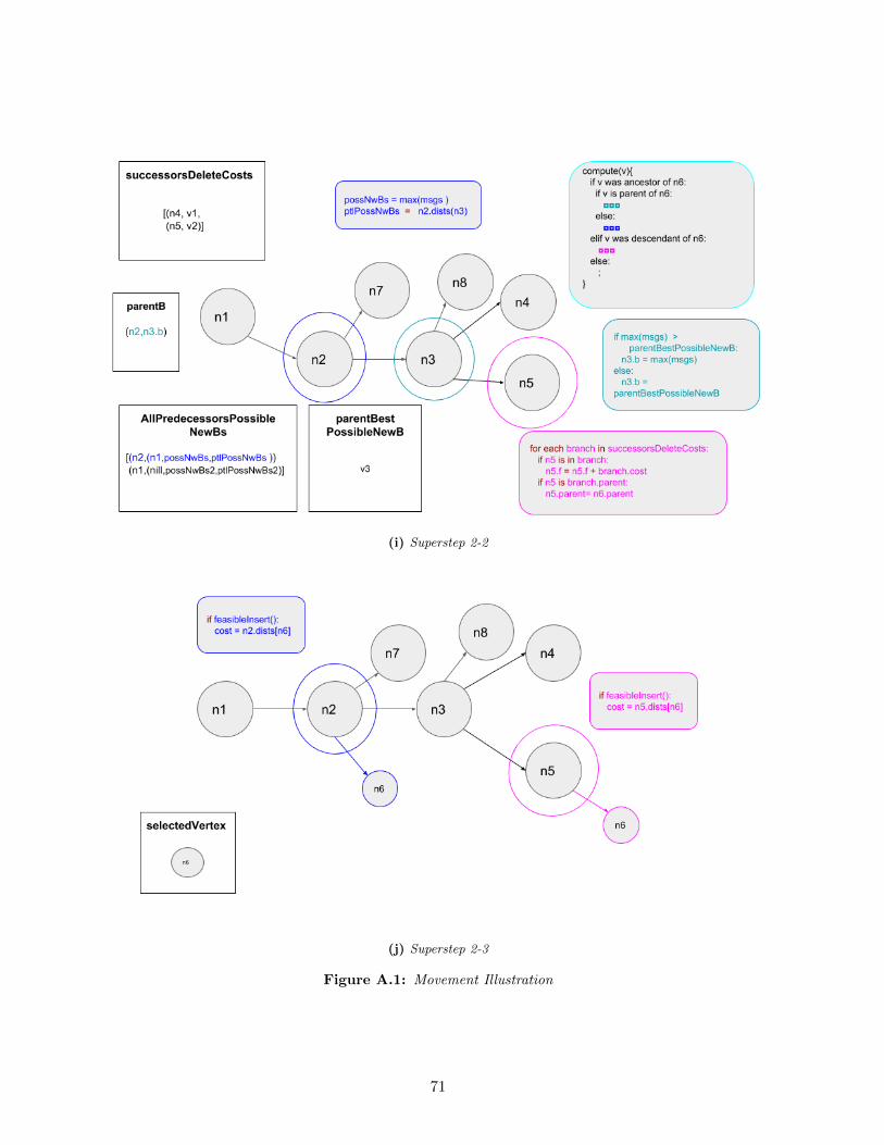
(i) Superstep 2-2
(j) Superstep 2-3
Figure A.1: Movement Illustration
71
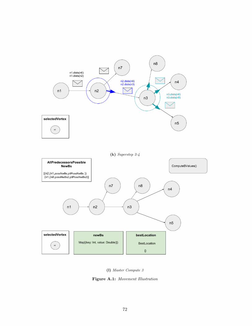
(k) Superstep 2-4
(l) Master Compute 3
Figure A.1: Movement Illustration
72
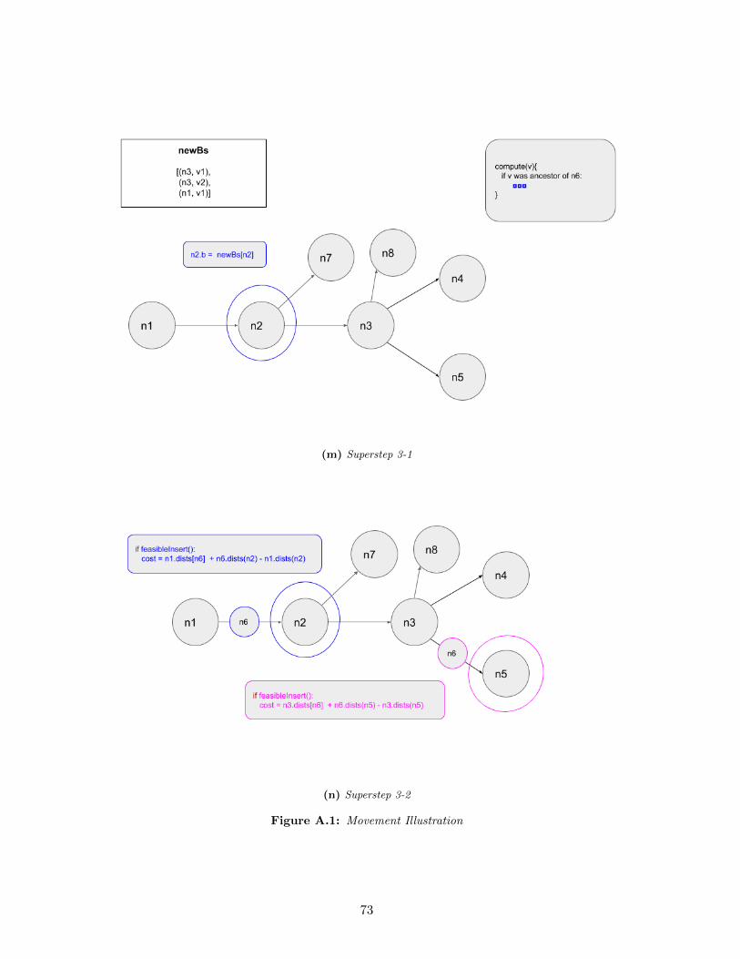
(m) Superstep 3-1
(n) Superstep 3-2
Figure A.1: Movement Illustration
73
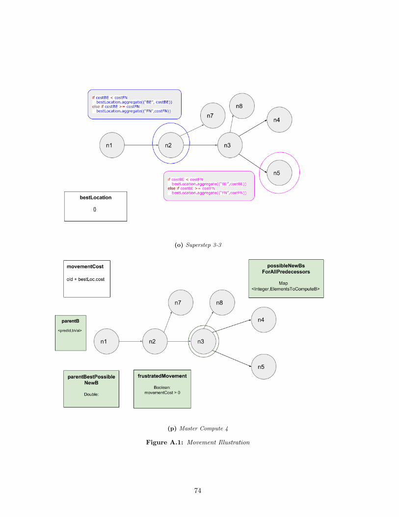
(o) Superstep 3-3
(p) Master Compute 4
Figure A.1: Movement Illustration
74

(q) Superstep 4-1
(r) Superstep 4-2
Figure A.1: Movement Illustration
75
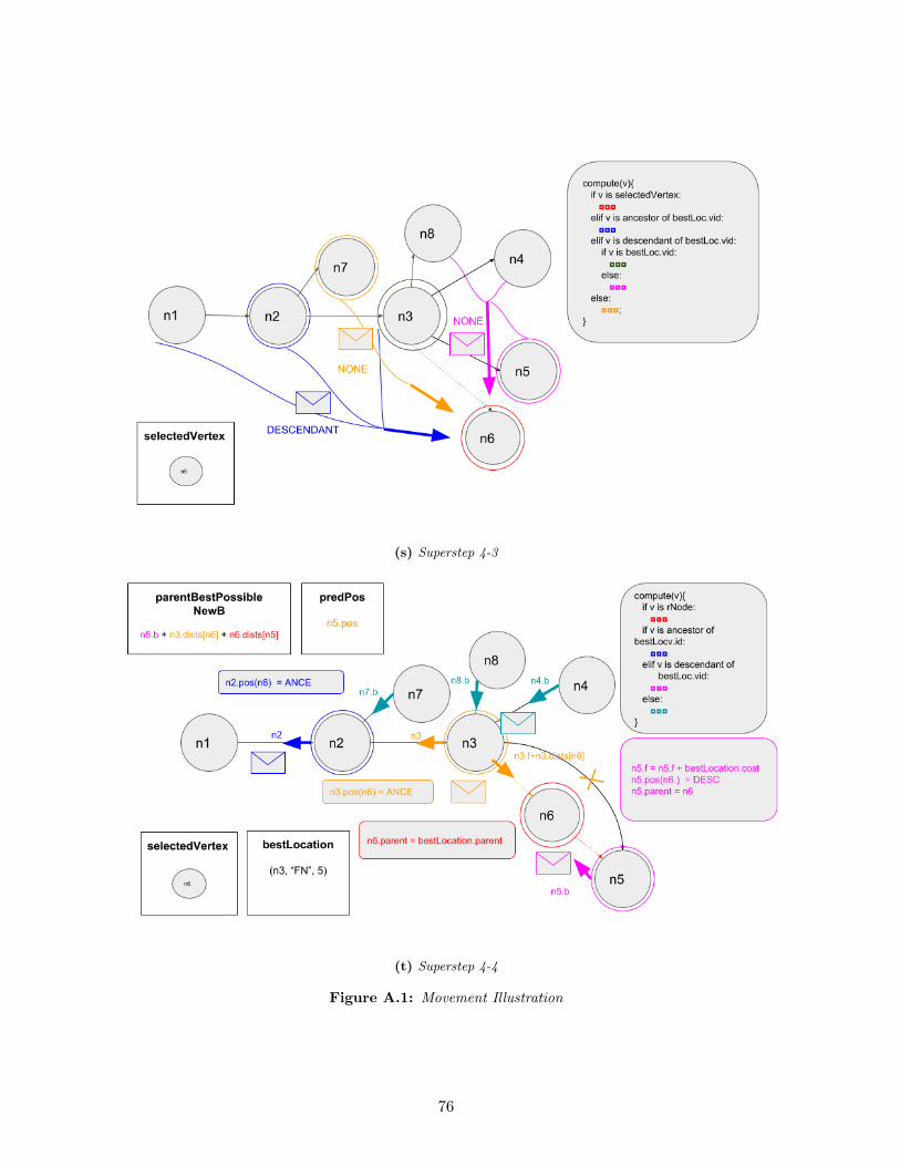
(s) Superstep 4-3
(t) Superstep 4-4
Figure A.1: Movement Illustration
76
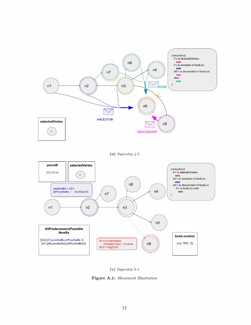
(u) Superstep 4-5
(v) Superstep 0-1
Figure A.1: Movement Illustration
77
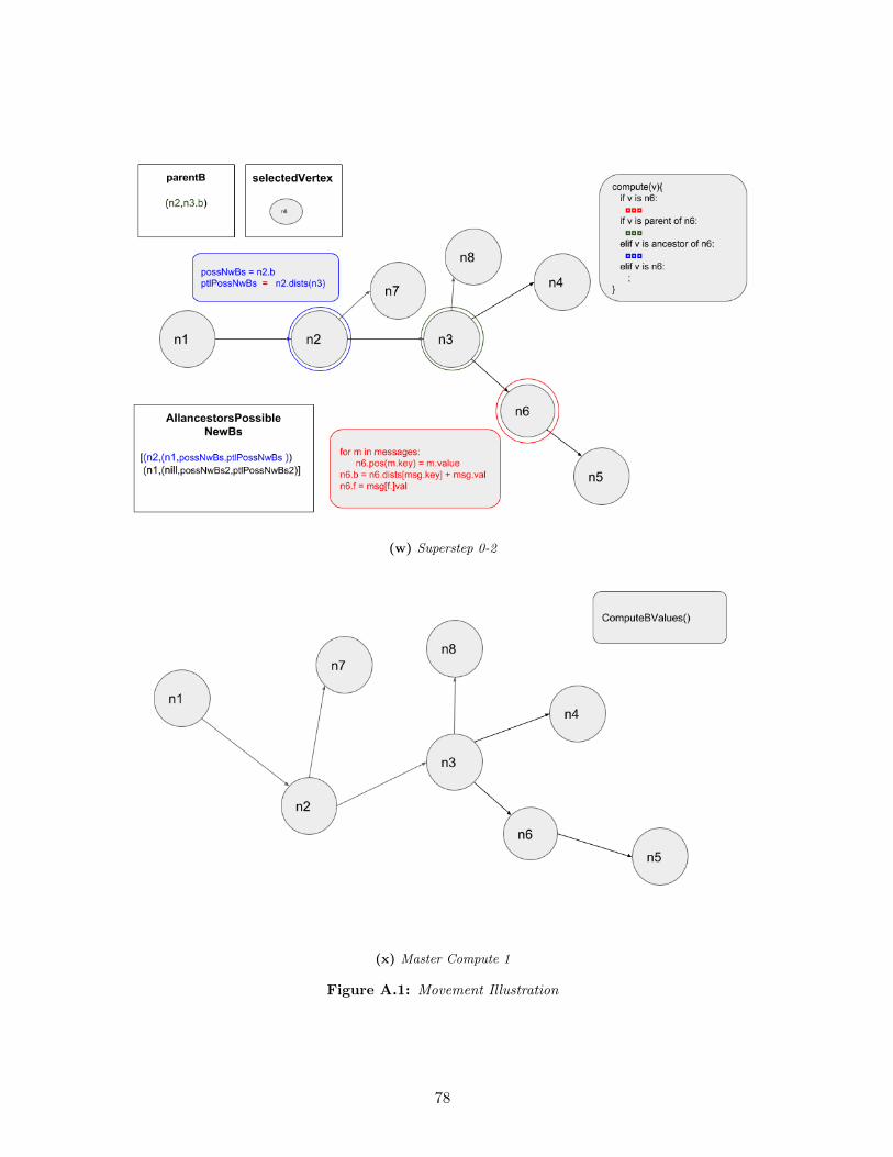
(w) Superstep 0-2
(x) Master Compute 1
Figure A.1: Movement Illustration
78
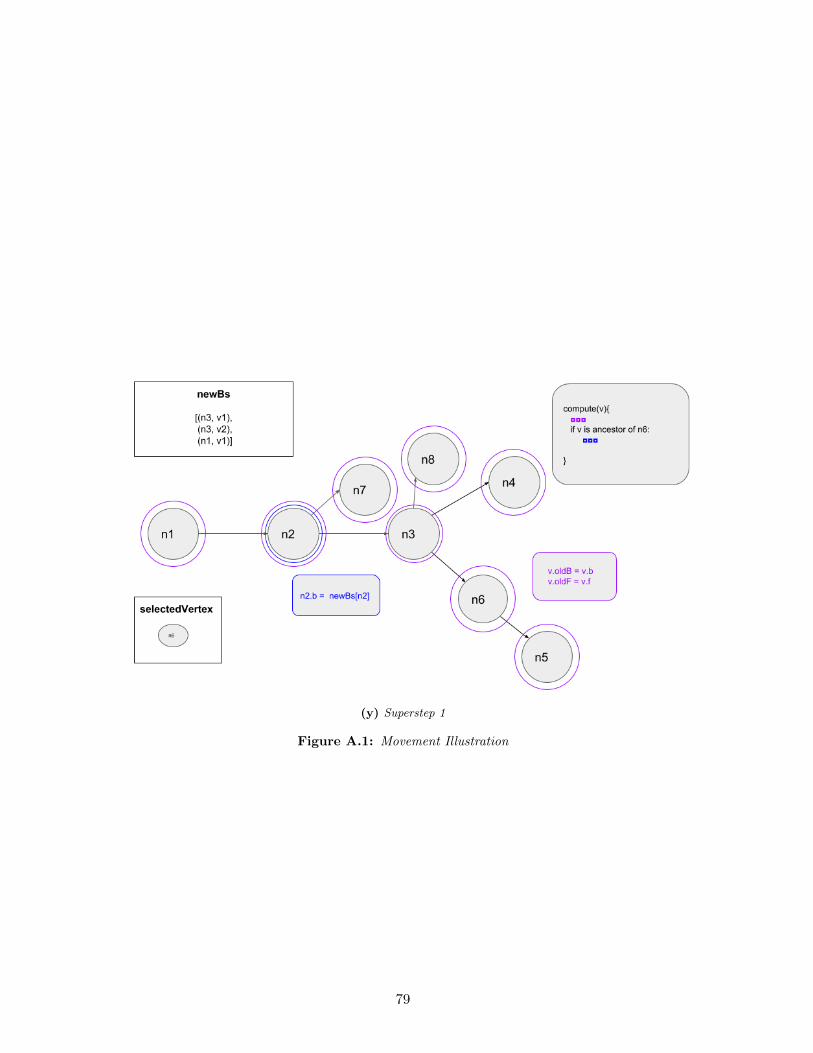
(y) Superstep 1
Figure A.1: Movement Illustration
79
Bibliography
[1] Alejandro Arbelaez, Deepak Mehta, Barry O’Sullivan, and Luis Quesada. A constraint-based
local search for edge disjoint rooted distance-constrained minimum spanning tree problem. In
Laurent Michel, editor, Integration of AI and OR Techniques in Constraint Programming: 12th
International Conference, CPAIOR 2015, Barcelona, Spain, May 18-22, 2015, Proceedings,
pages 31–46. Springer International Publishing, Cham, 2015.
[2] Roberto Battiti, Mauro Brunato, and Franco Mascia. Reactive search and intelligent optimiza-
tion, volume 45. Springer Science & Business Media, 2008.
[3] Martin Berlakovich, Mario Ruthmair, and Gunther R Raidl. A multilevel heuristic for the
rooted delay-constrained minimum spanning tree problem. In International Conference on
Computer Aided Systems Theory, pages 256–263. Springer, 2011.
[4] John W. Creswell. Research Design: Qualitative, Quantitative, and Mixed Methods Ap-
proaches. Sage Publications, 3rd edition, 2008.
[5] Geir Dahl, Luis Gouveia, and Cristina Requejo. On formulations and methods for the hop-
constrained minimum spanning tree problem. In Handbook of optimization in telecommunica-
tions, pages 493–515. Springer, 2006.
[6] Jason Eisner. State-of-the-art algorithms for minimum spanning trees-a tutorial discussion.
1997.
[7] Luis Gouveia, Ana Paias, and Dushyant Sharma. Modeling and solving the rooted distance-
constrained minimum spanning tree problem. Computers & Operations Research, 35(2):600
– 613, 2008. Part Special Issue: Location Modeling Dedicated to the memory of Charles S.
ReVelle.
[8] Safiollah Heidari, Yogesh Simmhan, Rodrigo N Calheiros, and Rajkumar Buyya. Scalable
graph processing frameworks: A taxonomy and open challenges. ACM Computing Surveys
(CSUR), 51(3):60, 2018.
80
[9] Marin Litoiu, Mary Shaw, Gabriel Tamura, Norha M. Villegas, Hausi A. Muller, Holger Giese,
Romain Rouvoy, and Eric Rutten. What Can Control Theory Teach Us About Assurances
in Self-Adaptive Software Systems? In Rogerio de Lemos, David Garlan, Carlo Ghezzi, and
Holger Giese, editors, Software Engineering for Self-Adaptive Systems III, volume 9640 of
LNCS, pages 90–134. Springer, 2017.
[10] Grzegorz Malewicz, Matthew H Austern, Aart JC Bik, James C Dehnert, Ilan Horn, Naty
Leiser, and Grzegorz Czajkowski. Pregel: a system for large-scale graph processing. In Pro-
ceedings of the 2010 ACM SIGMOD International Conference on Management of data, pages
135–146. ACM, 2010.
[11] Claudio Martella, Roman Shaposhnik, Dionysios Logothetis, and Steve Harenberg. Practical
graph analytics with apache giraph. Springer, 2015.
[12] Michael McCool, James Reinders, and Arch Robison. Structured parallel programming: pat-
terns for efficient computation. Elsevier, 2012.
[13] Juan C. Munoz-Fernandez, Gabriel Tamura, Raul Mazo, and Camille Salinesi. Towards a
requirements specification multi-view framework for self-adaptive systems. In 2014 XL Latin
American Computing Conference (CLEI), pages 1–14. IEEE, 2014.
[14] K.G. Murty. Linear programming. Wiley, 1983.
[15] Iksoo Pyo, Jaewon Oh, and Massoud Pedram. Constructing minimal spanning/steiner trees
with bounded path length. In European Design and Test Conference, 1996. ED&TC 96.
Proceedings, pages 244–249. IEEE, 1996.
[16] Mario Ruthmair and Gunther R Raidl. A kruskal-based heuristic for the rooted delay-
constrained minimum spanning tree problem. In International Conference on Computer Aided
Systems Theory, pages 713–720. Springer, 2009.
[17] Mario Ruthmair and Gunther R. Raidl. Variable Neighborhood Search and Ant Colony Opti-
mization for the Rooted Delay-Constrained Minimum Spanning Tree Problem, pages 391–400.
Springer Berlin Heidelberg, Berlin, Heidelberg, 2010.
[18] Mario Ruthmair and Gunther R Raidl. A memetic algorithm and a solution archive for the
rooted delay-constrained minimum spanning tree problem. In International Conference on
Computer Aided Systems Theory, pages 351–358. Springer, 2011.
[19] Sherif Sakr, Faisal Moeen Orakzai, Ibrahim Abdelaziz, and Zuhair Khayyat. Large-scale graph
processing using Apache Giraph. Springer, 2016.
81
[20] HF Salama, DS Reeves, and Y Viniotis. An efficient delay-constrained minimum spanning tree
heuristic. In Proceedings of the 5th International Conference on Computer Communications
and Networks, 1996.
[21] Gabriel Tamura. QoS-CARE: A Reliable System for Preserving QoS Contracts through Dy-
namic Reconfiguration. PhD Thesis, University of Lille 1 - Science and Technology and Uni-
versity of Los Andes, May 2012.
[22] Gabriel Tamura, Rubby Casallas, Anthony Cleve, and Laurence Duchien. QoS Contract
Preservation through Dynamic Reconfiguration: A Formal Semantics Approach. Science of
Computer Programming (SCP), 94(3):307–332, 2014.
[23] Tom White. Hadoop: The Definitive Guide. O’Reilly Media, Inc., 4th edition, 2015.
82
Recommended