
DO MUTUAL FUND MANAGERS HAVE SUPERIOR SKILLS?
An Analysis of the Portfolio Deviations from a Benchmark
by
Jean-François Guimond
Working Paper
December 2006
Please do not cite without permission. Comments welcome.
_______________________
Jean-François Guimond is assistant professor of finance at the Département de finance et assurance, Faculté des sciences de l’administration, Université Laval, bureau 3636, pavillon Palasis-Prince, Québec, Qc, Canada, G1K 7P4, 418-656-2131 ext. 12470, email: [email protected] This paper is based on my Ph.D. dissertation at Georgia State University. I thank my committee members: Stephen Smith (co-chair), Jason Greene (co-chair), David Nachman, and Richard Phillips. I also benefited from discussions with Jayant Kale and Patrick Savaria.

ABSTRACT
DO MUTUAL FUND MANAGERS HAVE SUPERIOR SKILLS?
An Analysis of the Portfolio Deviations from a Benchmark
By construction, actively managed portfolios must differ from those passively managed. Consequently, the manager’s problem can be viewed as selecting how to deviate from a passive portfolio composition. The purpose of this study is to examine whether we can infer the presence of superior skills through the analysis of the portfolio deviations from a benchmark. Based on the Black-Litterman approach, we hypothesize that positive signals should lead to an increase in weight, from which should follow that the largest deviations from a benchmark weight reveal the presence of superior skills. More precisely, this study looks at the subsequent performance of the securities corresponding to the largest deviations from different external benchmarks. We use a sample of 8385 US funds from the CRSP Survivorship bias free database from June 2003 to June 2004 to test our predictions. We use two external benchmarks to calculate the deviations: the CRSP value weighted index (consistent with the Black-Litterman model) and the investment objective of each fund. Our main result shows that a portfolio of the securities with the most important positive deviations with respect to a passive benchmark (either CRSP-VW or investment objective), would have earned a subsequent positive abnormal return (on a risk-adjusted basis) for one month after the portfolio date. The magnitude of this return is around 0.6% for all the funds, and can be as high as 2.77% for small caps value funds. This result is robust to all the performance measures used in this study.

Do mutual fund managers have superior skills? 1
DO MUTUAL FUND MANAGERS HAVE SUPERIOR SKILLS? :
An Analysis of the Portfolio Deviations from a Benchmark
1) INTRODUCTION
Do mutual fund managers have superior skills allowing them to do realize returns superior to that
of a passive benchmark on a risk-adjusted basis? This is an old issue in finance and for a long period of
time, the answer has been no1. More recent studies2, focusing on the trades made by mutual fund
managers, have uncovered evidence of superior skills. However, this new evidence answers a different
question. Instead of measuring the added value of active management over passive management, the
focus on the subsequent performance of trades is actually measuring whether the manager has improved
her previous position or not. Since the previous position of a fund is not, by definition, a passive
uninformed portfolio, the question about the added value of active management remains an open one.
By construction, actively managed portfolios must differ from passively managed ones,
regardless of how passive management is defined. Consequently, the manager’s problem can be viewed
as selecting how to deviate from a passive portfolio composition. The purpose of this study is to examine
whether we can infer the presence of superior skills through the analysis of the portfolio deviations from a
benchmark.
In a Bayesian setting, Black and Litterman (1992) have shown that positive information for a
given security will result in a higher weight in the optimal portfolio. This means that positive signals
should lead to an increase in weight, from which should follow that the largest deviations from a
benchmark weight reveal the presence of superior skills3. The rationale holds for both positive and
negative signals, and the largest negative signals should lead to the largest negative deviations.
1 Studies focusing on the returns of mutual funds, from Sharpe (1966), Jensen (1968), and Treynor (1965) to Malkiel (1995), have shown that actively managed funds have not earned abnormal returns or that, at best, they can recover their costs, explaining in part the growth in popularity of index funds. 2 E.g., Wermers (2000), Chen, Jegadeesh, and Wermers (2000), Pinnuck (2003), Alexander, Cici, and Gibson (2004). 3 Determining the source of the superior skills is beyond the scope of this study.

Do mutual fund managers have superior skills? 2
Since mutual funds cannot short sell, the strongest negative signal is not to hold a security, which
can be considered an active decision, just as the decision to hold a security. Even though negative signals
have the same weight in the portfolio (i.e. none), it is still possible to rank them. Indeed, not holding a
security that represents 5% of an index is a different decision than not holding a security that represents
only 0.1%.
Based on the Black-Litterman model, we test the null hypothesis that mutual fund managers have
no skills and make the following predictions: 1) if they have superior skills, then their largest absolute
deviations (including both positive and negative signals) will exhibit positive abnormal returns; 2) if they
have superior skills, the largest positive deviations will exhibit positive abnormal returns; and 3) if they
have superior skills, the difference between positive and negative deviations will exhibit positive
abnormal returns.
At the security level, deviations from a benchmark have been considered before in the literature,
but only from an internal benchmark, through the analysis of trades. Our study differs by looking at
deviations from an external benchmark. At the fund level, Wermers (2003) has studied the ex post
relationship between the deviations of the overall portfolio returns with respect to the S&P500 returns4
and the volatility of these deviations. This study looks at the subsequent performance of the securities
corresponding to the largest deviations from different external benchmarks.
We use a sample of 8385 US funds from the CRSP Survivorship bias free database from June
2003 to June 2004 to test our predictions. We use two external benchmarks to calculate the deviations:
the CRSP value weighted index (consistent with the Black-Litterman model) and the investment
objective5 of each fund (to consider the fact that most funds specialize in a subset of the CRSP universe).
Our main result shows that a portfolio of the securities with the most important positive
deviations with respect to a passive benchmark (either CRSP-VW or investment objective), would have
4 By considering the deviation of the overall portfolio return, this is equivalent to considering the deviation of all the securities in the portfolio. 5 The investment objective used reflects two dimensions: the market capitalization of the stocks held in the portfolio (large, mid, and small) and the investment style (blend, growth, and value).

Do mutual fund managers have superior skills? 3
earned a subsequent positive abnormal return (on a risk-adjusted basis) for one month after the portfolio
date. The magnitude of this return is around 0.6% for all the funds, and can be as high as 2.77% for small
caps value funds. This result is robust to all the performance measures used in this study.
Furthermore, our three predictions are verified in our sample, as the largest deviations seem to
indicate the presence of superior skills, but the largest positive deviations dominate.
Our results hold for all investment objectives, with the exception of large caps growth funds.
Also, contrary to the recent literature, the results are stronger for value funds and weaker for the growth
funds, on a risk-adjusted basis. This result is particularly interesting because it holds even when the
Fama-French or the Carhart model is used. In addition, the evidence on value funds is not driven by a
small cap effect, as the largest positive deviations of the large caps value funds also earn positive
abnormal returns.
Interestingly, the use of the corresponding investment objective index as the benchmark has
revealed that mutual funds tend to select a significant portion of their portfolio outside the index (up to
80% for value funds). Our results also show that these outside picks tend to drive the performance of the
largest positive deviations.
This study contributes to the literature by exploring subsets of the portfolio based on the idea that
active weights must deviate from passive benchmark weights. Overall, we provide evidence consistent
with the predictions based on the Black-Litterman model. To the best of our knowledge, this is the first
study to do so. Finally, our results support the idea that active managers do possess superior skills, but that
the constraints that they face obscure their detection through the analysis of overall returns.
The study is organized as follows. Section 2 reviews the literature. Section 3 develops the
hypotheses. Sections 4 and 5 present the data and methodology. Sections 6 and 7 present and discuss the
results, and section 8 concludes.
Do mutual fund managers have superior skills? 4
2) REVIEW OF THE LITERATURE
The search to find evidence that mutual fund managers possess superior skills, justifying the
existence of actively managed funds, is not a new one and the tools to investigate the question have
evolved through time.
The first studies have focused on the returns of mutual funds and, from Sharpe (1966), Jensen
(1968), and Treynor (1965) to Malkiel (1995), they have shown that actively managed funds have not
earned abnormal returns or that, at best, they can recover their costs, explaining in part the growth in
popularity of index funds.
These results are based on the study of actual portfolio returns. The main problem with using
actual portfolio returns is that they are affected by constraints faced by the manager, but their
performance is compared with benchmarks with fewer constraints, or constraints that are different. These
constraints include liquidity from investor flows6, tax considerations, legal limits or restrictions7, or
compensation incentives8 (e.g., benchmarking with other funds). Consequently, the aggregate
performance measures that are generally used may simply be inaccurate or unable to capture the
managers’ abilities, considering that they have little control over these constraints. Furthermore, the same
benchmark is imposed on all funds, regardless of both their individual constraints and investment
objective9.
In order to mitigate the mismatch between the constrained portfolio returns and the benchmarks,
two approaches are possible.
The first approach is to modify the benchmark in order to more appropriately reflect the
constraints of the portfolio. Some authors have adjusted the benchmark to reflect the specific investment
6 Edelen (1999) shows how the fund flows affect the returns. Rakowski (2002) also shows that the fund flow volatility negatively affects the performance of a fund. 7 For example, the funds face limits as to the fraction of outstanding shares that they can hold for a given security. Short-selling is also not permitted. 8 This issue will be discussed in section 5.1. 9 Lehmann and Modest (1987) study the importance of the benchmark portfolio and find that the performance measures are sensitive to the choice of the benchmark, when the same benchmark is applied to all funds. This has lead some authors [e.g., Daniel, Grinblatt, Titman, and Wermers (1997)] to develop customized benchmarks. This issue will be discussed in section 5.2.

Do mutual fund managers have superior skills? 5
objective of each fund [e.g., Daniel, Grinblatt, Titman, and Wermers (1997)], while others have
conditioned the performance measure on certain variables [e.g., Ferson and Schadt (1996) and Ferson and
Khang (2002)]. Finally, others have adjusted the benchmark in order to prohibit certain strategies to be
rewarded [e.g., Carhart (1997), Wermers (2000), Pinnuck (2003)]
With the exception of the last category, the effect of such adjustments is to improve the
performance of certain categories of managers, thus providing some evidence supporting active
management.
However, other important constraints, such as incentive contracts, liquidity provisions, flow of
funds, and taxes (also, marketing strategies and peer ranking), are not considered and would have to be
customized to each fund. It is not clear that we will ever get enough information to appropriately match
the constraints of each fund, when using all the portfolio composition.
The problem is twofold: first, it is difficult to account for these varying constraints (both over
time and across funds) in the design of an appropriate passive benchmark; and second, the manager has
little or no control over several constraints10.
The second approach focuses on removing the effects of some constraints on the returns. The
first constraint to be removed was the effect of transaction costs11. Although the results at the industry
level are not highly significant, this approach has uncovered some evidence that managers have superior
skills.
Since it is difficult to directly remove the effect of the other constraints, a solution to counter this
problem has been to identify a subset of the portfolio where the choices would be less affected by the
constraints. In other words, if managers have superior skills, where are we most likely to see evidence of
it? The only subset considered so far is the one containing stocks with a recent trading activity. This
10 E.g., Edelen (1999) has shown that the timing and the magnitude of the flows in and out of the fund have a negative effect on performance. 11 Hypothetical gross portfolio returns have been used by Grinblatt and Titman (1989), Grinblatt and Titman (1993), Grinblatt, Titman, and Wermers (1995), Malkiel (1995), Daniel, Grinblatt, Titman, and Wermers (1997), Chen, Jegadeesh, and Wermers (2000), Wermers (2000) and others.
Do mutual fund managers have superior skills? 6
approach has uncovered further evidence that managers may indeed possess superior skills12. This is
important, as for a long time, the literature had beaten up active portfolio management by demonstrating
the inability of active managers to outperform passive benchmarks or strategies.
However, there are some limitations as to the inferences that can be made from the evidence
uncovered by focusing on the trading activity. Instead of measuring the added value of active
management over passive management, the focus on the subsequent performance of trades is actually
measuring whether the manager has improved her previous position or not, because the reference
portfolio is internal (i.e. the fund itself). While making decisions that improve a position may increase the
likelihood of “beating” the benchmark, it is not guaranteed. In fact, it is not even a necessary condition,
as a fund could potentially beat the benchmark without improving its previous position. But the key point
here is that the previous position of a fund is not, by definition, a passive uninformed portfolio, leaving
the question about the added value of active management still open.
This study will focus on subsets of deviations with respect to an external benchmark. Trades can
be viewed as deviations from an internal benchmark. The other similarity with the study of the trading
activity is that the focus is also on a subset of the portfolio, as only the largest deviations will be
considered.
Finally, this study builds on Wermers (2003) who also looked at the deviations from an external
benchmark, but at the fund level, using the deviations of the portfolio return from the benchmark return.
His study focused on the ex post risk-return relationship of the portfolio return deviations. Our study will
consider the future performance of the largest deviations.
3) DEVELOPMENT OF HYPOTHESES
We will assume that the manager is maximizing the value of the fund and we will review the
potential effects of different objectives and constraints on the hypotheses in section 5.
12 E.g., Daniel, Grinblatt, Titman, and Wermers (1997), Chen, Jegadeesh, and Wermers (2000), Ferson and Khang (2002), Pinnuck (2003), and Alexander, Cici, and Gibson (2004).

Do mutual fund managers have superior skills? 7
By construction, actively managed portfolios must differ from passively managed ones,
regardless of how passive management is defined for now. Active management will then necessarily lead
to deviations from the benchmark weights. Consequently, the manager’s problem can be viewed as
selecting how to deviate from a passive portfolio composition.
There are essentially three approaches that can be taken by the manager to incorporate the signals
received from the available information13.
The first approach simply consists in using the information for choosing whether a security
should be over-weighted or under-weighted with respect to a passive benchmark (e.g., the S&P 500).
Under this approach, the deviation is the active decision made by the manager. However, this approach
does not guarantee that the resulting portfolio is optimal in any way.
A second approach consists in identifying undervalued securities and then decide how much to
invest in each one. If the manager believes in her ability (and her processing of the available
information), then she is more likely to put more money into stocks with higher positive information.
This should increase the likelihood of high deviations with respect to passive benchmark weights. But
this approach is not better than the first one to guarantee that the resulting portfolio is optimal in any way.
A third approach is to incorporate the private information in an optimization process in a mean-
variance setting. Black and Litterman (1992) propose such an approach. They argue that most investors’
views are relative and they propose to combine investors’ views with the market equilibrium. In a
Bayesian setting, they develop an approach where the optimal portfolios have the following properties14:
1) the unconstrained optimal portfolio is the market equilibrium portfolio plus a weighted sum of
portfolios representing an investor’s view; that is, the starting point of their model is the CAPM
equilibrium to which they add the private information signals of the investor; 2) the weight on a portfolio
representing a view is positive when the view is more bullish than the one implied by the equilibrium and
13 In this study, we will not seek to identify the source of the superior skills that the manager may have. Indeed, we will not try to see if the superior performance comes from private information or from a better processing of all sources of information. Consequently, the expression “private information” will refer to either information not publicly available and/or the “private” signal derived by the manager’s processing of public information. 14 He and Litterman (1999) present the intuition behind the Black-Litterman approach.

Do mutual fund managers have superior skills? 8
other views; 3) the weight increases as the investor becomes more bullish on the view as well as when the
investor becomes more confident about the view.
In other words, Black and Litterman (1992) have shown that positive information for a given
security will result in a higher weight in the optimal portfolio. This means that positive signals should
lead to an increase in weight, from which should follow that the largest positive deviations from a
benchmark weight reveal the strongest positive information possessed by the manager.
The rationale holds for both positive and negative signals, and the largest negative signals should
lead to the largest negative deviations.
Since mutual funds cannot short sell, the strongest negative signal is not to hold a security, which
can be considered an active decision, just as the decision to hold a security. Even though negative signals
have the same weight in the portfolio (i.e. none), it is still possible to rank them. Indeed, not holding a
security that represents 5% of an index is a different decision than not holding a security that represents
only 0.1%.
It is impossible to know exactly which approach is actually followed by the managers15.
However, regardless of the approach, the strongest signals of private information should show up in the
largest deviations. This should also be true regardless of the investment strategy, because what matters is
that a stronger signal of private information should lead to a larger weight (positive or negative), no
matter how the signal is obtained.
In order to consider the possibility that the largest deviations may be positive or negative, we will
look at the largest absolute deviations. In this study, the null hypothesis is that the manager does not have
any superior skills and that the abnormal return should be zero.
Based on the Black-Litterman model, our first prediction will be that, if managers have superior
skills, then a portfolio of their largest absolute deviations will exhibit a positive abnormal return. The
15 We do know however that the Black-Litterman approach is still used at Goldman Sachs and that other managers are likely to follow their approach as well. He and Litterman (1999) confirm that the model has gained wide applications. Also, most financial letters present their analysts’ recommendations in terms of deviation from a benchmark (e.g., overweight the energy sector and underweight the transportation sector).

Do mutual fund managers have superior skills? 9
portfolio will correspond to a long position in the securities with a positive deviation and a short position
in the securities with a negative deviation.
Since we hypothesize that the strongest signals are more likely to be the largest deviations,
focusing on the largest deviations has the power to detect superior ability if it exists. However, by
looking at the largest deviations, we are assuming that there is a monotonic relationship between the
deviations and the performance. Indeed, finding evidence of superior skills when focusing on the most
important deviations implies that they are expected to yield a higher performance. In other words, the
ordering of the deviations should be the same as for the performance. This implies that we will need a
two-step procedure to assess the validity of the largest deviations as a subset revealing the strongest
signals that the manager has. More precisely, we will test whether the largest deviations do better than
the entire portfolio. If true, then the monotonic relationship would be weakly respected.16
Focusing only on absolute deviations makes the implicit assumption that the positive and
negative signals have expected returns of opposite signs. However, if we decompose the difference
between the portfolio and the benchmark return [ ),(,11
),(,,),(, kttj
N
j
Bjt
N
ikttiit
Bkttkttp RwRwRR
ji
+==
+++ ∑∑ −=− ,
where wi,t is the weight of security i in the portfolio17 at time t, Bjtw is the weight of the security j in the
benchmark at time t, and Ri,(t,t+k) is the return of security i for the period between date t and t+k], we can
see that this assumption may lead to ambiguous results. Equation (1) provides the decomposition in
terms of deviations from an external benchmark.
44344214434421444 3444 21444 3444 21
?
0
?
)(
0
)(0
),(,
0
),(,),(,),(,
=
−
>
+
=
−+
>
− ∑∑∑∑=≠
+
=≠
+=
+−
=+
+
signportofliooutside
Rw
signbenchmarkoutside
Rw
signdeviationnegative
Rww
signdeviationpositive
Rwwi
jikttj
Bjt
jji
kttiitji
kttiBitit
jiktti
Bitit (1)
16 The relationship would be weakly respected because we will simply test the difference in the mean of the two groups, and not verify that the ordering is respected for all securities. 17 Note that the set of securities in the portfolio is not necessarily included entirely in the set of securities composing the benchmark. At the limit, they may even be mutually exclusive.

Do mutual fund managers have superior skills? 10
Intuitively, when the manager has a positive private signal, this should lead her to increase the
deviation of that position, and if the return is positive, then the combined effect produces a positive result.
Likewise, a negative private signal should lead to a negative deviation, and if the return is negative, then
the combined effect produces a positive result, indicating that the negative deviation was a good decision.
However, because we are considering two dimensions (the decision and the return), there is an
implicit assumption in our measure. In fact, we have the joint hypothesis that 1) positive information
leads (or is revealed by) to positive deviations, and 2) larger deviations must have higher returns.
A simple way of understanding the importance of this assumption is to realize that for a negative
deviation to be a good decision, the future return, (actual or abnormal) must be negative. Otherwise, if
the return is positive, then the measure will penalize the manager. The only reason why she should be
penalized is if the negative deviation had a higher return than the positive deviation. Otherwise, the
ordering was respected and the decision was not bad.
The main problem is that a negative deviation does not necessarily imply a negative subsequent
return. And the cause of this problem is that the sum of the deviations must add to zero, which means that
a positive signal leading to a positive deviation, must necessarily lead to a negative deviation somewhere
else. And this negative deviation is not motivated by any information other than the stock is not expected
to perform as well as the stock for which the deviation was increased positively.
For all these reasons, we have only two clear unambiguous predictions18. The first one is that, if
the manager has superior skills, the positive deviations (whether in the intersection or outside the
benchmark) should exhibit positive abnormal returns. The second one is derived from the monotonicity
assumption and is the following: if managers have superior skills, the difference between the positive and
negative deviations should exhibit positive abnormal returns.
18 Note that, in theory, if the signal leads to a decrease in deviation, then another deviation will necessarily be increased as a result. However, since short sales are not permitted for mutual funds, we will assume that positive signals are the source of most increases in deviations, and not the consequence of a negative signal. This point is not trivial, but it should be noted that, with the methodology developed in the next section, if the source of a positive deviation is a negative signal, it would actually work against finding evidence of superior skills.

Do mutual fund managers have superior skills? 11
Since the Black-Litterman model is based on the CAPM, a natural starting point to calculate the
deviations is to use the CRSP value-weighted index for the benchmark weights. However, the investment
objective of most funds is usually not as broad and restricts the choice of securities of the manager. It
also delimitates the reference point to which the manager’s performance is compared. For this reason, we
will also consider the index corresponding to the investment objective of the fund to calculate the
deviations.
We will also use a variety of subsets to capture the “largest” deviations. These will be described
in the next section. If we restate our predictions in terms of the largest deviations, this study will focus on
the following three predictions:
1) If managers have superior skills, then a portfolio of their largest absolute deviations should
exhibit a positive abnormal return.
2) If managers have superior skills, then a portfolio of the largest positive deviations (in the
intersection or outside the benchmark) should exhibit a positive abnormal return.
3) If managers have superior skills, then the difference between the largest positive and negative
deviations should exhibit a positive abnormal return.
Since the last two predictions are in fact the decomposition of the first one, testing them is likely
to reveal the source of the performance of the largest absolute deviations.
Finally, if there is a subset providing evidence that managers have superior skills, then it might
affect the overall return of the fund. Consequently, we might be able to use this information to predict, ex
ante, which funds are likely to do better for all holdings.
The next section presents exactly how each subset will be defined and which measures will be
used to compare them.

Do mutual fund managers have superior skills? 12
4) DATA AND METHODOLOGY
4.1) Data
The information on the characteristics of the mutual funds comes from the CRSP Survivor-Bias
Free US Mutual Fund Database (Sept. 2004 release). The information on the individual security returns
is from the CRSP database and the data necessary for the Fama-French three-factor model and Carhart
momentum model is from the Kenneth French’s internet data library. Finally, the information for the
exact composition of all the investment style indices is from Standard&Poor’s Research Insight Database.
The sample is based on the portfolio holdings information from June 2003 to June 200419. Only
funds with at least 50% of their holdings invested in domestic US equities are included. Since this study
is concerned with actively managed funds, index funds have been removed from the sample. Because
mutual funds usually have multiple classes, not all these funds have a distinct composition20. Taking all
the duplicates into account, 1751 funds21 are left in the sample with 8385 distinct portfolios from June
2003 to June 200422.
In order to use as many funds as possible, we have reconstructed the stock portfolio of all the
funds, i.e. all the holdings that were not US equity have been removed. Proceeding like this allows us to
focus on actively managed portfolios of stocks that can be compared with a passive portfolio of stocks. It
also eliminates the need to construct a passive portfolio that would appropriately consider the non-equity
holdings held in the funds.
19 In the CRSP Survivor-Bias Free US Mutual Fund Database, the holdings information is only available for portfolio dates starting in June 2003. 20 Several funds, within a same family, are exactly similar with respect to their portfolio composition. There are essentially four categories of funds that are replicates of each other: front load, deferred load, no load, and institutional. The first three categories are funds catering to individuals and the last one to institutional investors. In some cases, there may be more than one fund in a given category, but all the characteristics of the funds are the same except for the load factors, size and inception date. 21 The funds selected were funds for which it was possible to establish a relatively clear investment objective based on the market capitalization and the investment style. This selection was based in part on a sample drawn from the Morningstar Principia Pro database (version June 1999) and the rest was based on information found in the CRSP Survivor-bias free US mutual fund database. 22 The occurrence of each fund ranges from one to ten in the sample with 1596 funds appearing at least twice over 13 months.

Do mutual fund managers have superior skills? 13
Table 1 presents the characteristics of the sample based on the characteristics of the stocks held
by the funds (i.e. market capitalization and investment style).
[Insert Table 1 here]
This table highlights a number of interesting differences. The first one is that large cap funds
have fewer holdings than small cap funds. Large cap funds are also more concentrated than small cap
funds, as evidenced by their higher Herfindahl index.
Another interesting difference is that small cap funds tend to have a large number of their
holdings selected outside the composition of the index related to their investment objective. This number
is considerably less for large cap funds. The same relationship holds for the proportion of the portfolio
(in $) selected outside the index. This proportion is surprisingly high (around 80% for small cap funds
and 45% for large cap funds), which may reflect that managers are not really restricted by their
investment objective and/or there are more than two dimensions along which managers select their
securities. The proportion seems too high to be explained by the fact that the composition of the index
changes only twice a year on average. When the investment style is considered, the proportion selected
outside the index for value funds is higher than for growth and blend funds.
4.2) Methodology
Measures of performance
In this study, we compare the performance of different subsets of the portfolio, which will be
defined shortly. In order to compare the relative value of each subset, the same measure of performance
should be used for all subsets. Also, given that our ultimate goal is to detect the added value of active
management, the measure should use an external benchmark.
Essentially, the test is always to compare a portfolio of the securities included in a subset and to
compare the excess return or the abnormal performance with respect to a passive benchmark. So, the
question that we ask is: if we pick those securities that are part of a subset, and respect their relative
importance, could we beat a passive benchmark portfolio?

Do mutual fund managers have superior skills? 14
For each subset in the fund, we calculate the excess return as follows:
Bktktq
Q
q
Nqt RRw ++
=
−∑ ,1
where
∑=
= Q
qqt
qtNqt
w
ww
1
is the normalized weight of security q in the subset of Q securities,
ktqR +, is the security return23 from month t to t+k, and BktR + is the benchmark return.
Three benchmarks are considered for the excess returns: the CRSP value-weighted index, the
S&P500 and a custom benchmark based on the market capitalization of the fund24. Note that, in order to
reflect the private information of each fund, the relative importance of each security in each subset must
be preserved. This is achieved with the weight normalization procedure.
For each subset in the fund, we also calculate the abnormal performance as follows25:
[ ])( ,,1
Bktqtktq
Q
q
Nqt RERw ++
=
−∑
where ( )Bktqt RE +, is the expected return of each security q with the parameters evaluated at t.
23 Note that the subset return is a cumulative projected hypothetical return since we are making the assumption that the composition holds after the portfolio date t. 24 The custom benchmark reflects both the market capitalization (large caps, mid caps, and small caps) and the style (blend, growth, and value) of the securities in the funds. The following benchmarks are used: the S&P500 index for the large caps blend funds, the S&P500/BARRA growth index for the large caps growth funds, the S&P500/BARRA value index for the large caps value funds, the S&Pmidcap400 for the mid caps blend funds, the S&Pmidcap400/BARRA growth index for the mid caps growth funds, the S&Pmidcap400/BARRA value index for the mid caps value funds, the S&Psmallcap600 for the small caps blend funds, the S&Psmallcap600/BARRA growth index for the small caps growth funds, and the S&Psmallcap600/BARRA value index for the small caps value funds. 25 Note that this is similar to the selectivity measure by Daniel, Grinblatt, Titman, and Wermers (1997). The differences are that not all securities are considered (only those in the subset are) and that the expected return is not the characteristic-based benchmark that they develop.

Do mutual fund managers have superior skills? 15
For each security in the subset, the abnormal return is the actual return minus the projected (or
expected) return of the stock, i.e ( )Bktqtktqktq RERAR +++ −= ,,, . The following measures of expected
returns are used26:
1) ARq,t+k = Rq,t+k – [αq + βq Rm,t+k] (Market model) 2) ARq,t+k = [Rq,t+k – rf,t+k] – [αq + βq (Rm,t+k – rf,t+k)] (Jensen model) 3) ARq,t+k = [Rq,t+k – rf,t+k] – [αq + βq (Rm,t+k – rf,t+k) + γq HMLt+k + δq BMt+k] (Fama-French model) 4) ARq,t+k = [Rq,t+k – rf,t+k] – [αq + βq (Rm,t+k – rf,t+k) + γq HMLt+k + δq BMt+k + λq MOMt+k] (Carhart model) For each security, the return is evaluated using monthly data. The estimation period to calculate
the parameters of the different models is 60 months (with at least 30 months to enter the sample) prior to
each portfolio date.
The cumulative abnormal returns for the three projection periods (1, 3, and 6 months) are
calculated in the following manner:
CARq,p = ( ) 111
, −⎥⎦
⎤⎢⎣
⎡+∏
=
p
kkqAR
where p is the number of months in the projection and ARq,k is the monthly abnormal return.
The cumulative abnormal return for each subset is then pq
Q
q
Nqt CARw ,
1∑=
.
It is important to note that the unit of observation is at the fund level and that by specifying the
measure relative to a portfolio date at t, this study has a cross-sectional nature27, i.e. contrary to most other
studies28, the unit of observation is not a time-series of the fund returns.
Definition of subsets
As already mentioned, the performance measures are the same for each subset of the fund. The
definition of the subset will only identify the securities that will be used to form the subset portfolio. In 26 The same three benchmarks as for the excess returns are used for the market model specification. 27 There are 13 portfolio dates in our sample, from June 2003 to June 2004. The distribution of the observations by month is as follows: Jun03: 1337obs, Jul03: 515obs, Aug03: 522obs, Sep03: 1270 obs, Oct03: 153 obs, Nov03: 137 obs, Dec03: 897 obs, Jan04: 145 obs, Feb04: 350 obs, Mar04: 1115 obs, Apr04: 332 obs, May04: 407 obs, and Jun04: 1205 obs. 28 E.g., Daniel, Grinblatt, Titman, and Wermers (1997), Ferson and Khang (2002), and Pinnuck (2003).

Do mutual fund managers have superior skills? 16
order to test our predictions, we are using different types of deviations from a benchmark. The basic
deviation is defined as Bqtqt ww − , where wqt is the weight of the security q in the portfolio at time t and
Bqtw is the weight of the security in the benchmark. The absolute deviation is defined as B
qtqt ww − .
Scaled measures of deviations will also be used to express the relative importance of each deviation. Two
scales will be used. The first one is the ratio of the weight in the portfolio to the corresponding weight in
the benchmark: Bqt
qt
ww
(scale 1). The second one is the ratio of the deviation to the corresponding weight in
the benchmark: ( )
Bqt
Bqtqt
www −
(scale 2).
We use two different benchmarks to calculate the deviations. The first one is the CRSP value
weighted index and the second is the index corresponding to the investment objective of each fund. The
investment objective reflects the market capitalization and the style of the securities of each fund. The
specific indices used are the same as for the calculation of the performance based on customized market
models.
Some of the relative measures are not valid for the subsets using the investment objective as the
benchmark. More precisely, because a security can be chosen outside the investment objective index, the
relative measures are undefined for certain securities. For the scale 1 and the scale 2, the measures are
undefined when the security is outside the index, as the index weight is zero, making the measure infinite.
For most of these definitions, we will form subsets using the top 5, 10, and 15 securities (where
the rank is based on the different definitions of the deviations). To account for the problems with the
relative measures, we will also segment the securities to reflect the different composition of the portfolio
and the benchmark. More precisely, we will consider the securities in the portfolio only (outside the
index), those in the intersection, and those in the index only.
Because some of the subsets will use securities with no weight in the portfolio, it will not always
be possible to use the normalization procedure described above. In those cases, we will use equal weights

Do mutual fund managers have superior skills? 17
to form the subset normalized portfolio returns. This will mainly affect the subsets using either an
absolute deviation and/or a scale 2 measure.
Statistical tests
In order to test our predictions, we will perform three statistical tests. Test 1 will be a t-test of the
different measures of performance (gross returns, excess returns, and abnormal returns) for each of the
potential subsets29 likely to provide evidence of superior skills.
However, since we are using subsets of the portfolio, we must also verify that the performance of
the subset is better than the rest of the portfolio. Test 2 will then be a t-test of the difference between the
subset and the overall portfolio return30.
Finally, if there is a subset providing evidence that managers possess superior skills, then it might
be possible to use that information to see if we can identify ex ante the funds that will do better at the
overall level. Consequently, test 3 will consist in a comparison of the overall returns (using all holdings)
categorized according to the size of the deviations of the most revealing subset. In other words, the funds
will be ranked in decreasing order based on the size of the deviations at time t, quintiles (or deciles) will
be formed, and t-tests of the results by quintile (or decile) will be performed.
5) DISCUSSION OF THE METHODOLOGY
The purpose of this section is to come back on certain issues and discuss how they affect the
methodology presented in section 4.
29 This method of uncovering evidence of superior skills (with t-tests of means by grouping) has been used in the recent literature on the same topic, e.g., Daniel, Grinblatt, Titman, and Wermers (1997), Wermers (2000), Chen, Jegadeesh, and Wermers (2000), Badrinath and Wahal (2002), Pinnuck (2003), and Alexander, Cici, and Gibson (2004). 30 Since the overall portfolio return is a combination of the subset and its complement, comparing the subset to the overall return will give the same result as using the rest of the portfolio. Only the magnitude of the results is affected, as the sign of the difference is the same.

Do mutual fund managers have superior skills? 18
5.1) Objective function of the manager
In order to assess whether a mutual fund manager can add value over a passive management
strategy, it is necessary to consider what is the mission given to the manager. This is important as all
performance measures make implicit assumptions about it.
In a world with no information asymmetries between the agent (manager) and the principal
(investor), the delegation would lead the manager to make the same choices as would the investor. In this
case, the objective function of the manager would be to make choices that maximize the value of the fund.
However, in a world with information asymmetries, it is possible that the choices made by the manager
may not be optimal from the investor’s point of view. In addition to any information asymmetries, there
also exist incentive and operational constraints that the manager must consider. We will explain these
constraints below.
It is important to highlight that the manager’s maximization problem is usually not addressed
explicitly in the studies evaluating the performance of portfolio managers. This is so because the
evaluation is made from the investor’s perspective. At best, it is assumed, as mentioned in Wermers
(2000), that “The fundamental goal of a manager of an actively managed mutual fund is to consistently
hold stocks that have higher returns than an appropriate benchmark portfolio for the stocks31.”
In fact, the only literature explicitly considering the manager’s objective function is the one on
incentive contracts design. Recently though, incentive contracts have been considered in conjunction
with mutual fund performance [see Elton, Gruber, and Blake (2003)], but as a determinant of performance
and not as a constraint affecting the detection of superior ability (or the performance measure itself).
The ability of a manager of an actively managed fund is usually inferred by comparing the excess
return (adjusted for risk or not) of the fund with respect to some benchmark. So, from the manager’s
perspective, it would seem that her objective function is to maximize the value of the fund with respect to
some predetermined benchmark.
31 Note that the key word is “appropriate” which gives no information on the desired characteristics of the benchmark. Should it be on an excess return basis or on a risk-adjusted basis? Should it rule out strategies using public information or not?

Do mutual fund managers have superior skills? 19
However, as intuitive as this last statement may seem, Admati and Pfleiderer (1997) argue that
enforcing that constraint actually modifies the choices that the manager will make. Consequently, it is
important to differentiate between inferring ex post the ability of a manager with respect to some
benchmark and imposing the benchmark as an incentive in the objective function.
According to Admati and Pfleiderer (1997), if the objective function of the manager is to beat
some benchmark, AND if her compensation is tied to this benchmark, then her allocation will not be
optimal, from the investor’s perspective. The authors also look at the inferences that one can make about
using benchmarks to detect abnormal performance. Although the simple Bayesian model that they
develop tends to show some problems may be associated with tying the compensation to the benchmark,
they do not conclude that the usual approach of defining abnormal performance with respect to some
benchmark, will necessarily lead to incorrect inferences about the managers’ abilities32.
Incentive contracts are more common in the hedge fund industry as well as in the fixed-income
portfolio management industry. They however do exist in the mutual fund industry. In 1999, Elton,
Gruber, and Blake (2003) found that only a small fraction of the funds had explicit incentive contracts
(108 funds out of 6716).
It should be noted that, even if a manager does not have an explicit incentive contract to exceed a
benchmark, the constraint may still exist implicitly. Indeed, investors may have expectations that affect
their flow of money. If investors value past performance and invest in the best performing funds, then the
manager compensation function will become convex, as it is based on a fixed percentage of the assets
under management. This means that an unconstrained objective function, with implicit constraints, will
affect the portfolio choices as well.
However, incentive constraints are not the only ones to affect the manager’s maximization
problem. Almazan, Brown, Carlson, and Chapman (2004) study the effects of several operating
constraints and argue that they may serve as monitoring mechanisms to resolve some of the costs arising
32 In fact, on page 341, they state: “It is possible that assessments based on performance relative to a benchmark are good “rules of thumb” given the complexity of the Bayesian inference problem. However, examining the extent to which this might be true is beyond the scope of this article.”

Do mutual fund managers have superior skills? 20
from the principal-agent problem. They specifically consider the following operating restrictions
commonly found in the mutual fund industry: borrowing, short-selling, purchasing securities on margin,
holding individual security options, and trading in equity index futures.
Also, from the manager’s perspective, the flows of funds constitute operational constraints as she
has no control over these, and Edelen (1999) has shown that these flows negatively affect the measures of
performance.
Furthermore, Basak, Pavlova, and Shapiro (2003) provide an analysis of delegation in which
benchmarking practices may be welfare improving.
Operational constraints are important for three reasons. First, they may reduce the adverse effect
of incentive constraints. Second, they are beyond the control of the manager. And third, they affect the
choices and the performance of mutual funds.
The manager is also implicitly restricted (by some investors), at least ex post, on the information
set that she can use. Indeed, from a market efficiency perspective, several authors [e.g, Ferson and Schadt
(1996), Daniel, Grinblatt, Titman, and Wermers (1997)] argue that a manager should not be rewarded for
using strategies that can be replicated with public information. This is equivalent to imposing, ex post, a
minimum return constraint.
The purpose of this section was not to uncover the exact form of the objective function, but rather
to highlight the fact that different objectives and constraints will lead to different choices. At best,
constraints interact so that the optimal portfolio choices are the same from both the manager and the
investor point of view. At worst, constraints make the choices suboptimal from the investor’s
perspective. This implies that this problem should work against finding evidence of superior skills.
Nonetheless, one benefit of focusing on the top deviations is that they are less likely to be
affected by suboptimal choices, since they should represent the highest intensity of the manager’s skills.
So, if the objective function is different than the one assumed in section 3, it is mainly because of implicit
constraints which, if binding, should lead to suboptimal choices, making it more difficult to uncover
evidence of superior ability.

Do mutual fund managers have superior skills? 21
5.2) What is the appropriate benchmark?
This question is relevant mostly because the investment objective of a mutual fund is usually not
explicitly stated, or not always clearly determined. Indeed, when one looks into the Securities and
Exchange Commission prospectus of a fund, the information provided is usually insufficient to determine
what benchmark the fund is trying to “beat”. For certain funds, such as some Fidelity funds, the objective
to beat the S&P 500 is clearly stated. However, for a majority of funds, the information is provided in the
following format: invest 20-30% in bonds, invest 50-70% in US stocks, and invest 20-30% in
international stocks.
Having some idea of the composition, or even the exact composition of a fund, does not say much
about the objective being pursued. For example, the objective may be to outperform the S&P 500 and the
strategy may be to do so with small cap stocks. So, inferring that the appropriate benchmark to value the
active management is a small cap index would not be correct.
This ambiguity in the identification of the benchmark means that we have to guess what the
appropriate benchmark is.
One option is to assume the same index benchmark for all funds (e.g., the CRSP value-weighted
index). Another one is to assume the same benchmark strategy for all funds (e.g., the Fama-French
model) or the same set of public information [e.g., Ferson and Khang (2002)].
However, Lehman and Modest (1987) have shown that the choice of the benchmark is of primary
importance as it can, not only modify the magnitude of the abnormal performance, but also the ranking
among different funds. More recent papers [e.g., Brown and Goetzmann (1997)] have also argued that
the investment objective of the fund should be considered when choosing an appropriate benchmark.
Indeed, a one-size-fits-all benchmark may not capture the reality of the mutual fund industry as
funds tend to specialize into certain types of stocks or strategies. This is why customized benchmarks
have been proposed. Essentially, the idea is to attribute a different benchmark to each fund based on its
particular characteristics. The goal is to reflect the fact that not all funds are trying to “beat” the same
benchmark and that, consequently, applying the same benchmark to all funds is biasing the results.

Do mutual fund managers have superior skills? 22
It can then be an external benchmark based on the market capitalization of the stocks held by the
fund, such as the S&P500, S&Pmid400, S&Psmall600, or based on other dimensions, such as value vs
growth, etc. The customized benchmark can also be internally generated based on certain characteristics
of the stocks held in the fund. An example of such internally generated benchmark is the characteristic-
based benchmark33 developed by Daniel, Grinblatt, Titman, and Wermers (1997).
Having to guess what the benchmark is has two implications. The first one is to produce
potentially noisy measures of performance. And the second is that, even if we get positive results, they
are only as good as our guesses, as we do not know if we guessed correctly.
Once the appropriate benchmark has been determined, the next question is to decide which
dimensions should be considered in the performance measurement. The dimensions should be related to
the objective function of the manager (and the investors).
Different objectives are possible, but there are essentially two types that dominate the literature:
excess return (difference with the return of the benchmark) and risk-adjusted returns (difference adjusted
to reflect the difference in the mean and the variance)34. Note that we could also design benchmarks that
consider higher moments such as the skewness.
Even though most individual investors are happy to simply get a return that beats a benchmark
(usually some index), our goal in using risk-adjusted returns is to make sure that the performance of the
manager is not based on luck, i.e. it is based on superior skills.
5.3) The effect of time
So far, we have presented our analysis in a cross-sectional setting, i.e. considering each portfolio
composition (or set of decisions) at a given point in time as one observation. In a time-series setting, it is
the set of all decisions for the same fund through a period of time that is considered as one observation.
33 More precisely, the DGTW model is a customized benchmark based on the factors of the Carhart model. 34 To the best of our knowledge, when a fund explicitly states a benchmark to beat, it is only from an excess return basis only and never on a risk-adjusted basis.

Do mutual fund managers have superior skills? 23
What is important to realize is that when we are using time series, we are imposing a lot of factors
to be constant over time (e.g., the risk characteristics of the fund). We can see this as either adding a lot
of noise in the tests or imposing very strong restrictions on the management of the fund. By taking
averages of decisions over time, what we cannot capture is how those decisions reflected varying
constraints and information environments. Apart from the decision component itself, it also implies that
the risk-return profile of both the fund and the benchmark remained constant over the test period.
In order to solve these problems, conditional measures have been developed to account for the
dynamic behaviour of both the decision process and the environment [see Ferson and Schadt (1996) and
Ferson and Khang (2002)]. Conditional tests usually improve the performance of managers. Coggins
(2004) conditions the returns based on volatility and also gets results improving the performance of
managers.
Another problem with using times series is that it cannot account for the changes in managers that
inevitably take place over time. It also imposes the manager’s skill to remain constant over time, i.e. that
the manager does not learn more with experience. A new strand of the literature has considered this
problem and developed a database where the unit of observation is indeed the manager throughout her
career [see Baks (2003)].
Another way to get around the problems of time series is to develop a cross-sectional test that can
capture the essence of active management without imposing the restrictions of time series tests. In other
words, we should proceed with cross-sectional tests first before rejecting the existence of superior ability.
This is the approach taken in this study. However, time-series allow us to ask other relevant questions,
such as the persistence of superior skills should they exist. This topic is beyond the scope of this study.

Do mutual fund managers have superior skills? 24
5.4) Window dressing
An important issue that affects all studies using portfolio holdings at a given date and projecting
abnormal returns is the issue of window dressing35. It is important because all the measures are
dependent upon the reliability of the information. If the picture presented is not accurate, any conclusion
drawn from the data will be useless and false36.
Window dressing allegedly consists in modifying the portfolio composition of a fund for
cosmetic reasons, usually around reporting dates to impress or reassure investors. Although there are
anecdotal reports that it is a current practice, the empirical evidence uncovering it is rather mixed.
Window dressing is usually studied in conjunction with the January effect, as it might be
important enough to cause it. However, there are several other potential causes to the January effect.
Sias and Starks (1997) find that the January effect is primarily a result of individual investor
trading activity related to tax-loss selling rather than institutional window dressing. Lee, Porter, and
Weaver (1998) conclude that if the January effect is driven by institutional investors, it is not likely as a
result of window dressing. Lakonishok, Shleifer, Thaler, and Vishny (1991) examine the trading
activity of pension fund managers and do not find evidence of window dressing. Musto (1999) examines
yield patterns in the money markets at the turn of the year and finds evidence consistent with window
dressing by money market managers.
Carhart, Kaniel, Musto, and Reed (2001) examine whether mutual fund managers attempt equity
trades at the close of calendar quarters to temporarily inflate the net asset value and calendar quarter
returns37. They find that fund returns at calendar year-ends especially, and calendar quarter ends to a
35 Moskowitz (2000) mentions that window dressing may be a problem when projecting hypothetical returns. He finds evidence that could be consistent either with window dressing or tax-motivated trading. He also argues that the stock selectivity may be due to problems related to the turn of the year since it is positive only for that period. 36 Note that if managers are using derivative products to alter the characteristics of their portfolios, the indicated weights may not be representative of the real position. However, there is no information available to account for such usage. 37 They call this practice “leaning for the tape,” and it is commonly referred to in the financial press as “portfolio pumping.”

Do mutual fund managers have superior skills? 25
lesser extent, exhibit behaviour consistent with portfolio pumping. Note that portfolio pumping is also
consistent with window dressing if the funds’ fiscal years correspond with the calendar year.
O’Neil (2001) uses market-model residuals around fiscal year-ends. The residual are found to be
larger in magnitude and negative surrounding the days of a fiscal-year end than at other times of the year.
He argues that the results are consistent with the practice of window dressing.
However, Chen and Singal (2001) argue that several causes of the January effects are studied
individually, even though the evidence may be consistent with several hypotheses. The usual causes
studied are: tax-loss selling, window dressing, information, bid-ask bounce, or a combination of these. In
order to test window dressing, the authors focus on the stock returns of the June-July period, the period of
semi-annual reporting by institutional managers that is not contaminated by tax-related trading. They find
neither return patterns, nor volume patterns to be consistent with window dressing. Chen, Hong, and
Stein (2002) also do not find any significant tax effect, nor any window dressing effect.
It is thus not clear that window dressing exists and that it will affect the results of this study. It is
however an issue that needs to be addressed because the methodology relies on portfolio holdings and a
significant portion of the observations correspond to fiscal-year ends.
In this study, the window dressing issue is considered from a different angle. More precisely, if
window dressing is important, then we should not only see patterns in the returns, but it should also affect
the turnover ratio. Most studies so far have focused on the returns to detect the presence of window
dressing. While the turnover ratio is not really an indicator of window dressing per se, the window
dressing problem, by construction, cannot be significant for low turnover funds. Breaking down the
results by turnover ratio has the advantage of presenting a subset where the window dressing problem is
minimized and, considering that the majority of the portfolio dates correspond to quarterly reporting
dates, to potentially compare the importance of the problem for specific months, namely March, June,
September, and December. The goal is not to detect the presence of window dressing, but to find a way
to get results that are less likely to be affected by it.
Do mutual fund managers have superior skills? 26
Regardless of what has been mentioned so far, it is important to analyze the potential effects of
performing the evaluation with the wrong stocks (i.e. assuming that window dressing is present). The
detailed analysis is performed in Appendix A, but the general conclusion is that the proposed
methodology minimizes the likelihood that window dressing would bias our results favourably. This is
especially true for the subsets focusing on top deviations. Indeed, the main effect of window dressing is
probably to reduce the effect of extreme choices by moving the positions closer to the benchmark. The
choices potentially affected by window dressing are thus less likely to enter the subsets of extreme
choices, like the top deviations.
It is nonetheless possible that window dressing affects the results because several assumptions are
needed to conclude that it would be biasing only against finding something. However, considering that
the window dressing practice would have to affect all funds in the same manner, it can be argued that the
risk that the results will be due to window dressing is minimized, although not necessarily eliminated.
Indeed, the combination of conditions that must be met for window dressing to bias in favour of finding
superior performance when there is none, somehow reduces that probability38.
5.5) Survivorship bias
An important issue not yet discussed is the potential presence of survivorship bias that may be
introduced by not using a complete image of the industry, therefore potentially biasing the results.
Poor performing mutual funds are less likely to be observed in the data sets that are typically
provided by data providers. This so-called survivor problem can induce a substantial bias in measures of
the performance of the funds and the persistence of this performance. Many studies have recently argued
that survivorship bias can be avoided by analyzing a sample that contains returns on each fund up to the
38 Note that most studies using portfolio holdings to get abnormal returns do not attempt to qualify the effect of window dressing on their results. In fact, several authors [e.g., Daniel, Grinblatt, Titman and Wermers (1997), Wermers (2000), Kacperczyk, Sialm and Zheng (2003)] do not even mention the expression “window dressing” in their paper, even though the reliability of the portfolio composition is an assumption underlying all their measures and conclusions. Alexander, Cici, and Gibson (2004) is a notable exception.

Do mutual fund managers have superior skills? 27
period of disappearance using standard techniques. Such data sets are usually referred to as "survivorship
free".
What has been suggested to counter this problem is to constitute databases that include data about
funds that have disappeared [e.g., Elton, Gruber, and Blake (1996), Carhart, Carpenter, Lynch, and Musto
(2002)]. The Center for Research in Security Prices has even created such a database. However, Elton,
Gruber, and Blake (2001) find that another problem is created (an omission bias) that is as equally
important. The question is whether it is biasing for or against the results of this study.
It is not obvious how survivorship might actually influence the results as the approach does not
impose any existence period on the funds, nor does it consider specifically the past performance of a fund.
At the fund level, all that is really needed is a portfolio date and the portfolio composition. In fact, it is
the holdings of the funds that must exhibit some survival in order to calculate the abnormal performance
(which is prospective with respect to the portfolio date). So, the survival of the mutual funds themselves,
as generally discussed in the literature, is not really an issue. Instead, the issue might be that not all the
funds are in the sample, but there is no a priori reason to believe that the hypotheses tested should differ
for any particular subset of the industry.
6) PRESENTATION OF RESULTS
6.1) Largest absolute deviations
Table 2-AB presents the performance of all mutual funds for different subsets of the portfolio
based on the absolute deviations from a benchmark. Absolute deviations include either a long position in
the portfolio or a short position of stocks not in the portfolio. Since the subsets may include stocks
outside the portfolio (with a weight of zero), the subsets are based on equally-weighted portfolios of
securities forming the top absolute deviations.
[Insert Table 2-AB here]

Do mutual fund managers have superior skills? 28
The “all holdings” category represents the overall equity portfolio39. The calculated returns are
thus the projected hypothetical returns without transaction costs. On a gross return basis, the group of all
funds exhibits positive and significant performance. On an excess return basis, the returns are also
positive and significant, for all benchmarks and projection periods. When risk is considered, the
abnormal performance becomes negative and significant, which is in conformity with earlier studies of
mutual funds [e.g., Malkiel (1995)].
The performance of the top absolute deviations is generally negative and significant on an excess
return basis, but positive and significant on a risk-adjusted basis, for all the model specifications. There
are a few exceptions. First, the top absolute deviations provide stronger evidence when the deviations are
defined with respect to the investment objective rather than with respect to the CRSP universe. The
results are also stronger as the number of securities in the subset increases, as well as for the Fama-French
and Carhart models. The results are the same when a relative measure of absolute deviation (scale 2) is
used to rank the securities.
[Insert Table 2-CD here]
Table 2-CD presents the performance of the difference between the subsets in Table 2-AB and
the overall return of the funds. This is a weak test of the monotonicity of the top deviations with respect
to the rest of the portfolio. The results of this table confirm that the rest of the portfolio would not have
earned positive abnormal returns and that the top absolute deviations really provide evidence of superior
skills in our sample.
The decomposition of the results by investment objective shows that these results generally hold.
Unreported results reveal that this is however not the case for growth funds in general (regardless of the
market capitalization). Blend funds and value funds do much better. This is especially true for small caps
value funds for which we report the results in Table 3-AB.
[Insert Table 3-AB here]
39 These portfolios do not correspond to the real portfolios without transaction costs, but only to the domestic equity portion of the real portfolios. All the non-domestic equity securities have been removed (i.e. cash, bonds and international stocks).

Do mutual fund managers have superior skills? 29
In section 3, we mentioned that the predictions based on absolute deviations were ambiguous as
the sign of the performance of the negative deviations could be either positive or negative. This might
explain the unintuitive pattern that we observe between the excess returns and the abnormal returns.
Indeed, the results between the two groups of performance measures are systematically opposite. The
equal-weighting procedure may also contribute to the ambiguity of these results. Also, considering all the
possible negative deviations may not reflect the constraints imposed on the manager. Indeed, a lot of
small stocks may not be sufficiently traded.
Absolute deviations include either long position of the stocks in the portfolio or short position of
stocks not in the portfolio. Our results indicate that the largest deviations (regardless of the sign) would
have earned a positive return on a risk-adjusted basis. The next sections will decompose these deviations
to find out if the abnormal performance is driven by the selection or the non-selection of stocks. We will
first look at the largest positive deviations and then at the difference between the largest positive
deviations and the negative deviations.
6.2) Largest positive deviations
Table 4-AB presents the performance of all mutual funds for different subsets of the portfolio
based on the positive deviations from a benchmark. On an excess return basis, all the subsets exhibit
positive and significant returns. On a risk-adjusted basis, the results are positive and significant for the
one month projection period for the top 5 positive deviations. This is true for all performance measures.
This result also holds for different definitions, e.g., the top 5 positive deviations w.r.t. the CRSP index,
the top 5 positive deviations w.r.t. the investment objective index, and top 5 positive deviations for the
securities chosen outside the investment objective index (i.e. only in the portfolio). These results
generally hold also for top 10 and top 15 positive deviations for the one month projection period,
although these results are not reported. The abnormal performance ranges from 0.37% to 0.94% for one
month.
[Insert Table 4-AB here]

Do mutual fund managers have superior skills? 30
It is interesting to note that the most important positive deviations within the securities in both the
portfolio and the index (intersection) have negative and significant returns while those outside the index
(Portfolio only) have positive and significant returns. This might be caused by the fact that funds tend to
select a significant portion of their portfolio outside the index (as shown in Table 1). This would imply
that managers seek to differentiate themselves by selecting outside the index and seem to be successful at
it, based on this sample. This result also indicates that the largest positive deviations may not be in the
intersection, and that the abnormal performance may be driven by those securities selected outside the
index.
Table 4-CD presents the performance of the difference between the subsets in Table 4-AB and
the overall return of the funds. Almost all the subsets considered do better than the overall return, which
confirms the results in Table 4-AB. Again, the largest positive deviations in both the portfolio and the
index have either a negative or a lower positive performance with respect to the entire portfolio.
[Insert Table 4-CD here]
The decomposition of the results by investment objective shows that these results generally
hold40. The tables reveal that this is however not the case for the large caps growth funds. Blend funds
and value funds do much better. This is especially true for small caps value funds for which we report the
results in Table 5-AB. For example, the abnormal performance ranges from 2.04% to 2.76% for one
month.
[Insert Table 5-AB here]
In addition to larger abnormal returns, the results for small caps value funds generally extend to
the three month projection period. The top 5 relative deviations (scale 1) with respect to the CRSP value
weighted index, also exhibit positive and significant abnormal returns for all the models.
Table 5-CD presents the performance of the difference between the subsets in Table 5-AB and
the overall return of the funds. It clearly shows that the largest deviations in the intersection do not
perform as well as the largest deviations chosen outside the index. 40 The results are not reported.

Do mutual fund managers have superior skills? 31
[Insert Table 5-CD here]
The results in this section are consistent with the prediction that was made in section 3, i.e. the
largest positive deviations should exhibit positive abnormal returns, if managers have superior skills.
6.3) Largest positive minus negative deviations
The results obtained for the absolute deviations were also generally consistent with the presence
of superior skills. We have seen in the last section that the largest positive deviations were also consistent
with the presence of superior skills. This is not sufficient to claim that the largest positive deviations
were driving the results for the largest absolute deviations. In order to do so, we must compare the largest
positive deviations with the negative deviations. Since the top 5 positive deviations subset is the
definition for which we get the most consistent results, we will use it to represent the largest positive
deviations subset and compare it to negative deviations. The results of this comparison are presented in
Table 6-AB.
[Insert Table 6-AB here]
The results indicate that, for the one month projection, the largest deviations do better than the
negative deviations. This is true for different definitions of negative deviations41. When we decompose
the results by investment objective42, the results still hold, but the largest deviations for small caps value
funds exhibit are even more convincing, as shown in Table 7-AB. The results hold for almost all
definitions and projection periods.
[Insert Table 7-AB here]
The evidence from this sample thus seems to indicate that the largest positive deviations were
greatly influencing, if not driving, the results of the largest absolute deviations. Our results show an
interesting similarity with the evidence based on trades. With trades, entry and exit seems to convey
41 To represent all the negative deviations, we consider four possibilities: 1) all the negative deviations in both the portfolio and the index; 2) all the negative deviations in the portfolio only; 3) all the negative deviations in the index only, using the index weights to construct the portfolio of negative deviations; and 4) same as in (3) but using equal weights to construct the portfolio of negative deviations 42 The results are not reported.

Do mutual fund managers have superior skills? 32
more information43. These are the largest deviations from an internal benchmark. Our results also imply
that the largest deviations from an external benchmark are conveying more information
6.4) Predictive value of the subsets
In the previous section, our results have shown that selecting the securities with the largest
positive deviations with respect to a passive benchmark would yield a significant positive abnormal
performance. An important argument for focusing on subsets of the portfolio to uncover the presence of
superior abilities was that the overall returns were affected by all the constraints faced by the manager.
And these constraints may obscure the detection of superior skills. Now that we have found evidence
consistent with the presence of superior skills, it is only logical to see if we can use this information to
identify, ex ante, the funds with the best overall returns.
A simple way to test this is to, first, rank all the funds based on the sum of top 5 positive
deviations at time t (the portfolio date), form quintiles or deciles, and then perform t-test of the average
overall performance of each grouping. Table 8 presents the performance of the hypothetical returns when
the funds are ranked based on their top 5 positive deviations. The results show that the top 5 positive
deviations do not seem to have any predictive value in our sample. Segmenting the funds by investment
objective does not reveal any predictive value44.
[Insert Table 8 here]
7) DISCUSSION OF RESULTS
7.1) Effect of the procedure for ranking In this study, we have used two external benchmarks to rank the different deviations. The Black-
Litterman model, which provides the theoretical foundation for our approach, is based on the CAPM.
This means that the CRSP value weighted index is the only optimal index consistent with the model.
43 See Alexander, Cici, and Gibson (2004). 44 The results are not reported.

Do mutual fund managers have superior skills? 33
Indeed, it is difficult to argue that the investment objective index (which a subset of CRSP value weighted
index based on the same relative market capitalization) constitutes an optimal index. However, most
funds specialize in a subset of the CRSP universe45.
As we have seen in the previous section, the choice of the index does not materially affect the
main conclusion, i.e. the top positive deviations exhibit positive abnormal performance. But the use of
the investment objective index has revealed that most of this abnormal performance can be attributed to
securities selected outside the index of reference, something that cannot be revealed by the use of the
CRSP value-weighted index.
7.2) Effect of the investment objective
Our sample reveals that the main result is that the one month future performance of the top 5
positive deviations (both with respect to CRSP or the investment objective) is positive and significant for
all investment objectives (with the exception of the large caps growth funds).
In our sample, we also find that value funds do better and that growth funds do worse. This is
different than the results usually reported in the literature. For example, Daniel, Grinblatt, Titman, and
Wermers (1997) find that aggressive-growth funds exhibit some selectivity ability. Chen, Jegadeesh, and
Wermers (2000) find that growth-oriented funds have unique skills in identifying underpriced large-
capitalization growth stocks. Kosowski, Timmermann, White, and Wermers (2001) use a bootstrap
analysis and find that the performance of the best and worse funds is not due to luck and that the growth-
oriented funds show superior performance.
There are a few reasons that may explain our different result. First, the fund investment
objectives used in this study differ from other studies. For example, we use the Morningstar
categorization which uses nine categories based on the market capitalization (large, mid, and small) and
the investment style (blend, growth, and value). This is somewhat different from the aggressive growth,
45 In fact, for practical reasons such as the liquidity of a stock, all funds end up specializing in a subset of the CRSP universe.

Do mutual fund managers have superior skills? 34
growth, growth and income, and balanced funds used in other studies [e.g., Wermers (2000), Chen,
Jegadeesh, and Wermers (2000)]. For these reasons, the results of this study may not be directly
comparable, as only domestic equity funds are used.
Second, because the growth category in this study is broader than in the rest of the literature, it
may explain why the results are different. However, it should be pointed out that the mid caps and small
caps growth funds also provide evidence of superior skills, but with less intensity than the value funds. If
aggressive growth funds invest primarily in small caps, then this evidence would be consistent with the
existing literature.
Another reason that may explain our different result is the measure of performance used. In all
the studies finding evidence of superior skills with growth funds, the measure of performance is the
DGTW (1997) characteristic-based benchmark mentioned before. Because this measure is based on the
previous security weights of the portfolio, the benchmark in this measure is therefore internal, which is
different from our approach based on an external benchmark.
Interestingly, the results for value funds hold regardless of the market capitalization (large, mid,
and small caps) of the stocks held in the fund. This means that the market capitalization does not seem to
affect the likelihood that managers possess private information. More precisely, even though there is
more public information available for large caps stocks46, which should reduce the importance of
abnormal returns based on private information, managers are still able to profit from their private
information. This means that active management may still be a relevant strategy for investors willing to
invest in large caps stocks.
In our sample, most funds are present more than once and some of them show up to ten times.
Although it is not clear how this might influence the results, we have verified our findings by using funds
that appeared no more than two times in our sample. Considering that the time between the two
46 These stocks are also more closely followed by analysts, reducing further the possibility of abnormal performance based on private information.

Do mutual fund managers have superior skills? 35
observations is most likely six months47, the possibility of autocorrelation (or overlap) between
observations from the same fund is eliminated, because we only project for six months. With 379
observations, the results still hold48.
Finally, our evidence may simply show that managers following a value strategy build their
portfolio differently than those who follow a growth strategy. Maybe it pays more to deviate more with
value stocks than with growth stocks.
7.3) Effect of the deviation definition
The main difference between absolute deviations and positive deviations is that positive abnormal
performance is present for the three projection periods for the absolute deviations and mostly for the one
month projection with the positive deviations. However, because of the ambiguity of the predictions
based on absolute deviations, the basis of comparison may not be appropriate.
As for using straight deviations or different scales for relative deviations, the main results do not
seem to be qualitatively affected when the ranking is done with respect to the investment objective.
However, the results do seem more consistent for straight deviations. There is no a priori reason to
believe that one should do better. In fact, it is mostly dependent on how the managers make their decision
about the extent of deviation from the benchmark weight. If they think in terms of the impact on the
overall portfolio return, they might focus on straight deviations. This approach might be easier to
rebalance the portfolio and decide which stocks will decrease in importance.
But if they think in terms percentage deviations, then scaled measures may capture more.
However, this makes the rebalancing a little more complicating as a percentage increase in one security
will not lead directly to a similar decrease (in percentage) in another one. For practical reasons, straight
deviations may then provide more consistent evidence across different categories of funds. This may
47 Mutual funds must disclose their portfolio composition semi-annually to the Security and Exchange Commission. 48 We have also considered funds present no more than four times in the sample (1629 observations) and the results are qualitatively the same.

Do mutual fund managers have superior skills? 36
explain why the relative deviations with respect to the CRSP index do not reveal much, except for small
caps value funds.
7.4) Effect of the projection period
At the overall level, the positive abnormal performance generally holds for the one month
projection period, but the results are usually negative and significant for the three and six months
projection period49. These results seem to indicate that there is a limited period for which the superior
ability persists, as we observe a reversal of abnormal performance through time.
In unreported results, we have explored the effect of the reporting frequency for the funds in our
sample50. We get the same result for higher frequencies than with lower frequencies, which seems to
indicate that the largest positive deviations provide evidence of some persistence in the ability.
The pattern highlighted in the results suggests that the forecasting ability of the managers only
last one month. If these results indicate the true ability of the managers, then they would be justified to
rebalance their portfolio more frequently to capture the gains from their forecasting ability. We should
then observe that the funds with a high turnover do better. However, in unreported results, the high
turnover funds do not seem to make better forecasts for longer projection periods, even if they have
higher abnormal performance for the one month projection.
It is tempting to relate the overall negative mutual funds to the reluctance of managers to sell their
stocks, since their prediction ability seems to be better for very short term horizons. However, we must
not forget the limits of our methodology.
Our methodology projects hypothetical buy-and-hold portfolios, i.e. we make the assumption that
the composition of the portfolio will remain the same for the entire projection period. Considering that
49 There are some exceptions, e.g. the mid caps and small caps value funds, where the positive abnormal performance may hold for three and six months as well. 50 The frequencies that we have considered range from one (the most recent portfolio composition as of June 2004) to ten. However, it should be noted that only 8 funds have reported 10 times (33 funds have reported 9 times), but these 8 funds all belong to the same family of funds. Also, the frequency is not uniform throughout the sample period. For example, some funds may have reported on a quarterly basis in 2003 and on a monthly basis in 2004.

Do mutual fund managers have superior skills? 37
the median turnover ratio ranges from 52% to 123%, the importance of this assumption is not trivial and
seriously limits the credibility of the projection for longer periods. This means that the reversals that we
observe for our hypothetical portfolios may not be present in actual portfolios. However, the credibility
of the projection for one month is higher as the changes to the portfolio composition are less likely to be
important over a small period of time51. Our projected returns are also based on the assumption that the
estimated parameters for the models are stable through time and valid for longer horizons.
Only monthly time-series of portfolio composition will enable us to truly see if the managers
have the ability to take advantage of the reversal effect that we observe in the projected returns.
7.5) Window dressing
All the studies using the portfolio composition of mutual funds are potentially subject to the
window dressing problem. In section 5, we argued that clear evidence (i.e. that cannot be explained by
something else) has yet to be found and that, if present, window dressing should work against finding
evidence of superior information52.
We also argued that the window dressing potential bias could be minimized by looking at the
results for low turnover funds, where window dressing is less likely to be important, by construction. In
unreported results, the main result, that the top positive deviations subset provides evidence of superior
private information (on a risk-adjusted basis), also holds for low turnover funds53.
Another place to look for evidence of window dressing is the portfolio composition date54.
However, the main problem with the portfolio dates is that the number of funds per portfolio date is not
uniformly distributed. In our sample, the dates with the most observations are March, June, September, 51 This is especially true for funds with large positions in a stock. Indeed, they may decide to modify their position over a longer period of time. 52 Indeed, if the manager has superior private information, then modifying the composition for cosmetic reasons (not information-based) would decrease the likelihood of earning abnormal returns. Also, selecting the most important deviations minimizes the problem as window dressing would probably move the active weight closer to its passive benchmark weight, thereby decreasing the likelihood of being included in the top. 53 This is true for the entire range of turnover, i.e. from funds with turnover below 25 (1241 funds) to funds with a turnover above 150 (1423 funds). It should also be mentioned that the results are better for high turnover funds. This is consistent with Wermers (2000) who finds that high turnover funds have better performance. 54 The results are not reported.

Do mutual fund managers have superior skills? 38
and December. These represent the most common dates at which the funds disclose their portfolio
composition, and they also correspond to fiscal year-end for most funds. The observations for the other
months most likely represent funds that disclose their information on a monthly basis. Since it is
supposed that window dressing is more likely to take place at fiscal year-end dates, we have segmented
the data in two groups: the funds reporting in March, June, September, and December (5824
observations), and the funds reporting in other months (2561 observations). The results for the two
groups are similar, i.e. the largest positive deviations earn positive and significant abnormal returns for
the one month projection period and for all performance measures. These results do not support the
presence of window dressing.
For all these reasons, we believe that the likelihood that our results are driven by window
dressing effects is very low.
8) CONCLUSIONS
Do mutual fund managers have superior skills? Since active management must deviate from
passive management, our hypothesis was that, if they have superior skills, the largest deviations should
exhibit positive abnormal performance. We find evidence consistent with this hypothesis. More
precisely, we find that the top 5 positive deviations from the corresponding investment objective index
exhibit positive abnormal performance on both an excess return and risk-adjusted basis for a one month
projection period. The top 5 absolute deviations also provide evidence of superior skills, but the evidence
is somewhat ambiguous and seems to be driven by the largest positive deviations. This result is
reinforced by the fact that the largest positive deviations do better than the negative deviations.
In our sample of 8385 mutual funds, the main result holds for all the investment objectives
considered (with the exception of the large caps growth funds). The results are strongest for the value
funds, and the weakest for growth funds, which is in sharp contrast with previous studies where growth
funds are usually providing the best results. It should be noted that the evidence in these studies is based
on trades, which compares the portfolio weights with an internal benchmark. In this study, we compare

Do mutual fund managers have superior skills? 39
them to an external benchmark. The results for value funds are reinforced by the fact that they hold even
with the Fama-French and the Carhart models.
In our sample, the results do not seem to be affected by window dressing or survivorship bias.
We have also used two external benchmarks and a variety of deviation definitions, without altering the
results qualitatively. Furthermore, we have found no evidence that using this information could be used
to identify ex ante the funds most likely to earn the best overall returns.
Our sample also reveals that mutual funds tend to select most of their stocks outside the
composition of their corresponding investment objective index (e.g., up to 80% on average for value
funds). This is important as the most important picks outside the index seem to provide a positive
abnormal performance, as well as driving the overall results.
This study contributes to the literature in several ways. It is the first one to explore new subsets
of the portfolio based on the idea that active weights must deviate from passive benchmark weights. To
the best of our knowledge, it is also the first empirical test of the Black-Litterman model. Our results are
also consistent with managers following the portfolio management approach described in Black and
Litterman (1992). This evidence supports the idea that active managers do possess superior skills, but
that the constraints that they face obscure their detection through the analysis of overall returns.
The evidence of superior information found in this study is based on a cross-sectional approach
and is based on one year of data. Further research will look at time-series to search for the persistence of
the ability through time.
REFERENCES Admati, A. R. and P. Pfleiderer, 1997, Does it All Add Up? Benchmarks and the Compensation of Active Portfolio Managers, Journal of Business, Vol. 70, No. 3 Alexander, Cici, and Gibson, 2004, Does Motivation Matter When Assessing Trade Performance? An Analysis of Mutual Fund, Working Paper Almazan, A., K. C. Brown, M. Carlson, and D. A. Chapman, 2004, Why Constrain your Mutual Fund Manager? Journal of Financial Economics,

Do mutual fund managers have superior skills? 40
Badrinath, S. G. and S. Wahal, 2002, Momentum Trading by Institutions, Journal of Finance, Vol. 57, No. 6 Baks, K. P., 2003, On the Performance of Mutual Fund Managers, Working Paper, Emory University Basak, S., A. Pavlova, and A. Shapiro, 2003, Offsetting the Incentives: Risk Shifting and Benefits of Benchmarking in Money Management, Working Paper, December Black, F. and R. Litterman, 1992, Global Portfolio Optimization, Financial Analysts Journal, Vol. 48, No. 5 Brown, S. and W. Goetzmann, 1997, Mutual Fund Styles, Journal of Financial Economics, 43, 373-399 Carhart, M., 1997, On Persistence in Mutual Fund Performance, Journal of Finance, Vol. 52, No. 1 Carhart, M. M., J. N. Carpenter, A. W. Lynch, and D. K. Musto, 2002, Mutual Fund Survivorship, Review of Financial Studies, Vol. 15, No. 5, Winter, p. 1439-1463 Carhart, M. M., R. Kaniel, D. K. Musto, and A. V. Reed, 2001, Leaning for the tape: Evidence of gaming behavior in equity mutual funds, Journal of Finance Chen, H., C. Hong and J. Stein, 2002, Breadth of ownership and stock returns, Journal of Financial Economics, Vol. 66, p. 171-205 Chen, H-L, N. Jegadeesh, and R. Wermers, 2000, The Value of Active Mutual Fund Management: An Examination of the Stockholdings and Trades of Fund Managers, Journal of Financial and Quantitative Analysis, 35 Chen, H. and V. Singal, 2001, What drives the January Effect?, Working paper, Virginia Tech Coggins, F., 2004, Évaluation de la performance des fonds mutuels lorsque les mesures de risque sont conditionnelles à l’information publique (Mutual fund performance evaluation when the risk measures are conditional on public information), Ph.D. Dissertation, Université Laval Daniel, K., M. Grinblatt, S. Titman, and R. Wermers, 1997, Measuring Mutual Fund Performance with Characteristic-Based Benchmarks, Journal of Finance, Vol. 52, No. 3 Edelen, R. M., 1999, Investor Flows and the Assessed Performance of Open-End Mutual Funds, Journal of Financial Economics, Vol. 53 Elton, E. J., M. J. Gruber, and C. R. Blake, 1996, Survivorship Bias and Mutual Fund Performance, Review of Financial Studies, Vol. 9, No. 4, Winter, p. 1097-1120 Elton, E. J., M. J. Gruber, and C. R. Blake, 2001, A First Look at the Accuracy of the CRSP Mutual Fund Database and a Comparison of the CRSP and Morningstar Mutual Fund Databases, Journal of Finance, Vol. 56, No. 6, December, p. 2415-2430 Elton, E. J., M. J. Gruber, and C. R. Blake, 2003, Incentive Fees and Mutual Funds, Journal of Finance, Vol. 58, No. 2

Do mutual fund managers have superior skills? 41
Ferson, W. and R. Schadt, 1996, Measuring Fund Strategy and Performance in Changing Economic Conditions, Journal of Finance, Vol. 51 Ferson, W. and K. Khang, 2002, Conditional Performance Measurement Using Portfolio Weights: Evidence for Pension Funds, Journal of Financial Economics, Vol. 65 Grinblatt, M. and S. Titman, 1989, Mutual Fund Performance: An Analysis of Quarterly Portfolio Holdings, Journal of Business, Vol. 62, No. 3 Grinblatt, M. and S. Titman, 1993, Performance Measurement without Benchmarks: An Examination of Mutual Funds Returns, Journal of Business, Vol. 66, No. 1 Grinblatt, M., S. Titman, and R. Wermers, 1995, Momentum Investment Strategies, Portfolio Performance, and Herding: a Study of Mutual Fund Behavior, American Economic Review, Vol. 85 He, G. and R. Litterman, 1999, The Intuition Behind Black-Litterman Model Portfolios, Goldman Sachs Investment Management Research Jensen, M. C., 1968, The Performance of Mutual Funds in the Period1945-1964, Journal of Finance, Vol. 23, No. 2 Kacperczyk, M., C. Sialm, and L. Zheng, 2003, On the Industry Concentration of Actively Managed Equity Mutual Funds, Working paper, University of Michigan Kosowski, R., A. Timmermann, H. White, and R. Wermers, 2001, Can mutual fund stars really pick stocks? New evidence from a bootstrap analysis, Working paper Lakonishok, J., A. Shleifer, R. Thaler, and R. Vishny, 1991, Window dressing by pension fund managers, AEA Papers and Proceedings, 227-231 Lee, C. F., D. C. Porter, and D. G. Weaver, 1998, Indirect Indirect Tests of the Haugen-Lakonishok Small-Firm/January Effect Hypotheses: Window Dressing versus Performance Hedging, Lehmann, B. and D. Modest, 1987, Mutual Fund Performance Evaluations: A Comparison of Benchmarks and Benchmark Comparisons, Journal of Finance, Vol. 42 Malkiel, B. G., 1995, Returns from Investing in Equity Mutual Funds 1971 to 1991, Journal of Finance, Vol. 42, 233-265 Moskowitz, T. J., 2000, Discussion of Mutual Fund Performance: An Empirical Decomposition into Stock-Picking Talent, Style, Transactions Costs, and Expenses, Journal of Finance, Vol. 55, No. 4 Musto, David K., 1999, Investment decisions depend on portfolio disclosures, Journal of Finance 54, 935-952 O=Neil, E. S., 2001, Window dressing and equity mutual funds, Working Paper Pinnuck, M., 2003, An Examination of the Performance of the Trades and Stock Holdings of Fund Managers: Further Evidence, Journal of Financial and Quantitative Analysis, Vol. 38, No. 4, December Rakowski, D., 2002, Fund Flow Volatility and Performance, Working Paper, Georgia State University

Do mutual fund managers have superior skills? 42
Sharpe, W. F., 1966, Mutual Fund Performance, Journal of Business, 39 Sias, R. W. and L. T. Starks, 1997, Institutions and individuals at the turn-of-the-year, Journal of Finance 52, 1543-1562 Treynor, J. L., 1965, How to Rate Management of Investment Funds, Harvard Business Review, Vol. 43 Wermers, R., 2000, Mutual Fund Performance: An Empirical Decomposition into Stock-Picking Talent, Style, Transactions Costs, and Expenses, Journal of Finance, Vol. 55, No. 4 Wermers, R., 2003, Are Mutual Fund Shareholders Compensated for Active Management “Bets”?, Working paper, University of Maryland

Do mutual fund managers have superior skills? 43
APPENDIX A Analysis of the potential effects of window dressing in this study
The goal of this section is to analyze the potential effects of performing the evaluation with the
wrong stocks, i.e. assuming the presence of window dressing. Note that if managers have some ability, it
means that any replacement stocks (chosen for cosmetic reasons) should do more poorly than the original
stock.
There are two cases to consider: the case of the entire portfolio and the case of subsets. In the
first case, if a stock is in the portfolio, it should be either because the manager has no information or
because she has some positive information, assuming that the composition reflects a selection process. If
she sells a stock for cosmetic reasons and buys it back after the portfolio date, it has to be that she
believes that the stock has more potential than the replacement stock, otherwise, she would not buy it
back. So, on average, she expects the replacement stock to earn a lower abnormal period in the future.
Consequently, any projection using the window dressed portfolio should not do as well as the real
portfolio, if managers have superior ability of course.
Note that this does not mean that the replacement stock should earn negative abnormal returns,
but simply that the abnormal returns should be lower. So, if managers have some ability, then using the
window dressed portfolio should reduce the abnormal performance of the funds. If they do not, then it
could be that the replacement stock will turn out to be better and give the impression that the results will
be better. Although this can be possible for a particular fund, it is not obvious that it would necessarily
lead to a bias towards finding abnormal performance when there is none.
As for the top deviations, they are less likely to be affected as the main effect of window dressing
is probably to modify the weight to make it closer to the benchmark weight. Focusing on top deviations
(whether relative or absolute) minimizes the effect of window dressing on these subsets.

Do mutual fund managers have superior skills? 44
Note also that the preceding analysis assumes that the proceeds of the stocks sold for cosmetic
reasons are actually reinvested in stocks, but the fund may simply hold the proceeds in cash. In this case,
the effect of window dressing would also bias the results against finding superior performance, assuming
that managers do have superior ability.
It is nonetheless possible that window dressing affects the results because several assumptions are
needed to conclude that it would be biasing only against finding something. However, considering that
the window dressing practice would have to affect all funds to consistently affect the results, it can be
argued that the risk that the results will be due to window dressing is minimized, although not necessarily
eliminated. Indeed, the combination of conditions that must be met for window dressing to bias in favour
of finding superior performance when there is none, somehow reduces that probability.

Do mutual fund managers have superior skills? 45
Table 1 - Descriptive statistics by market capitalization and investment style
Category # obs SizeTurnover
ratioExpense
ratio % cash % equityNumber of
holdings Herfindahl
Number of holdings
(intersection)
Weight holdings
(intersection)
Number of holdings (outside index)
Weight holdings (outside index)
Mean 607.33 94.36 1.46 3.82 94.80 111.24 20.13 38.87 41.84% 72.37 58.16%Std. dev. 2975.58 111.95 0.56 5.07 6.21 151.13 15.12 57.92 28.82% 116.31 28.82%
Min 1.01 0.00 0.10 0.00 50.49 10.00 0.73 0.00 0.47% 0.00 0.80%Max 77951.90 2322.00 5.26 47.38 111.07 3277.00 466.52 817.00 99.20% 2476.00 99.53%
Median 75.70 68.48 1.35 2.34 96.58 80.00 17.13 23.00 27.45% 51.00 72.55%Mean 856.16 77.86 1.41 3.24 95.52 90.07 23.35 46.26 54.13% 43.81 45.87%
Std. dev. 3951.18 78.74 0.59 4.41 5.87 84.46 12.86 56.72 28.52% 51.12 28.52%Min 1.01 0.00 0.12 0.00 52.28 10.00 2.00 0.00 0.47% 0.00 0.80%Max 77951.90 1359.00 4.71 42.07 111.07 994.00 229.33 482.00 99.20% 667.00 99.53%
Median 80.00 59.00 1.29 1.95 97.25 69.00 20.15 32.00 65.11% 29.00 34.89%Mean 355.91 113.63 1.49 3.93 94.46 98.36 17.62 25.02 23.68% 73.34 76.32%
Std. dev. 999.07 132.63 0.51 4.72 6.21 68.29 10.32 39.32 16.89% 50.65 16.89%Min 1.10 0.00 0.19 0.00 53.70 19.00 2.89 0.00 2.58% 3.00 1.58%Max 11332.70 2235.00 4.24 44.31 104.34 651.00 104.48 380.00 98.42% 566.00 97.42%
Median 60.05 82.00 1.38 2.73 96.21 84.00 14.94 16.00 20.52% 63.00 79.48%Mean 297.24 113.10 1.54 4.88 93.64 161.74 15.60 34.15 20.19% 127.60 79.81%
Std. dev. 947.36 142.25 0.52 6.22 6.64 250.69 19.83 68.09 11.89% 194.86 11.89%Min 1.03 0.91 0.10 0.00 50.49 11.00 0.73 0.00 1.11% 1.00 1.55%Max 29967.60 2322.00 5.26 47.38 106.74 3277.00 466.52 817.00 98.45% 2476.00 98.89%
Median 78.00 82.00 1.45 3.05 95.34 105.00 12.27 18.00 17.54% 83.00 82.46%Mean 471.12 84.33 1.38 3.94 94.74 148.09 18.43 83.30 72.52% 64.79 27.48%
Std. dev. 2462.88 79.86 0.55 5.23 6.23 259.15 11.24 102.51 23.03% 189.28 23.03%Min 1.01 0.00 0.12 0.00 52.07 10.00 0.73 0.00 7.53% 0.00 0.80%Max 66873.30 965.00 4.50 47.38 104.09 3277.00 101.98 817.00 99.20% 2476.00 92.47%
Median 83.65 66.48 1.26 2.30 96.57 86.00 15.68 51.00 82.41% 24.00 17.59%Mean 571.27 116.80 1.54 3.49 95.44 98.63 20.97 34.70 48.28% 63.93 51.72%
Std. dev. 2524.19 124.97 0.59 4.69 5.31 83.14 17.73 31.36 25.58% 68.44 25.58%Min 1.06 0.00 0.10 0.00 53.05 11.00 1.67 0.00 1.11% 2.00 6.88%Max 77951.90 2235.00 4.71 46.95 111.07 1011.00 466.52 341.00 93.12% 834.00 98.89%
Median 72.90 87.00 1.41 2.20 96.94 80.00 17.44 27.00 55.78% 48.00 44.22%Mean 738.71 70.35 1.41 4.18 93.98 105.74 20.04 17.41 17.07% 88.32 82.93%
Std. dev. 3723.11 104.06 0.52 5.42 7.14 127.27 13.18 22.39 6.34% 107.03 6.34%Min 1.03 0.00 0.17 0.00 50.49 10.00 1.55 0.00 0.47% 7.00 49.56%Max 68573.10 2322.00 5.26 45.39 100.00 1764.00 229.33 279.00 50.44% 1522.00 99.53%
Median 73.45 52.00 1.32 2.63 96.14 77.00 17.60 12.00 16.71% 63.00 83.29%
Value 2829
Blend 1719
Growth 3837
Mid 1610
Small 2291
All 8385
Large 4484

Do mutual fund managers have superior skills? 46
Table 1 - Descriptive statistics by market capitalization and investment style (continued)
Category # obs SizeTurnover
ratioExpense
ratio % cash % equityNumber of
holdings Herfindahl
Number of holdings
(intersection)
Weight holdings
(intersection)
Number of holdings (outside index)
Weight holdings (outside index)
Mean 569.08 77.51 1.34 3.30 95.66 112.51 21.25 88.24 83.83% 24.27 16.17%Std. dev. 3103.87 70.14 0.56 4.55 5.62 119.56 11.75 89.67 10.20% 46.32 10.20%
Min 1.01 1.00 0.12 0.00 56.50 10.00 5.81 9.00 32.41% 0.00 0.80%Max 66873.30 490.00 4.50 35.48 104.09 994.00 101.98 482.00 99.20% 533.00 67.59%
Median 84.60 59.00 1.25 1.81 97.40 77.00 17.86 60.00 86.12% 15.00 13.88%Mean 848.23 89.54 1.50 2.93 96.14 80.69 25.55 47.53 68.51% 33.16 31.49%
Std. dev. 3472.44 80.96 0.64 4.13 5.09 69.11 12.89 35.54 11.65% 39.98 11.65%Min 1.06 0.00 0.36 0.00 59.00 14.00 5.73 3.00 16.30% 2.00 6.88%Max 77951.90 762.18 4.71 41.00 111.07 722.00 113.93 341.00 93.12% 387.00 83.70%
Median 86.20 70.00 1.34 1.67 97.53 65.00 21.94 41.00 70.09% 22.00 29.91%Mean 1059.65 64.20 1.36 3.57 94.67 86.05 22.14 16.37 19.35% 69.68 80.65%
Std. dev. 4879.14 79.38 0.53 4.60 6.74 68.19 13.15 14.17 5.67% 55.48 5.67%Min 1.10 0.00 0.17 0.00 52.28 10.00 2.00 0.00 0.47% 7.00 49.56%Max 68573.10 1359.00 3.64 42.07 100.00 776.00 229.33 128.00 50.44% 667.00 99.53%
Median 72.40 51.00 1.26 2.26 96.80 71.00 19.62 13.00 18.53% 57.00 81.47%Mean 329.75 76.60 1.39 4.91 92.73 117.02 16.58 58.59 50.61% 58.43 49.39%
Std. dev. 715.74 54.81 0.48 5.51 7.36 92.27 10.26 78.96 25.19% 48.66 25.19%Min 1.10 0.00 0.19 0.00 55.59 24.00 3.36 3.00 7.53% 3.00 1.58%Max 7194.10 253.00 3.39 44.31 100.00 489.00 51.12 380.00 98.42% 322.00 92.47%
Median 66.90 60.20 1.28 3.50 95.32 102.00 12.65 33.00 39.16% 47.00 60.84%Mean 377.34 145.18 1.56 3.66 95.26 98.77 17.06 22.29 23.44% 76.48 76.56%
Std. dev. 1114.05 162.83 0.56 4.47 4.60 65.11 10.48 18.08 8.99% 52.47 8.99%Min 1.10 4.24 0.49 0.00 73.04 19.00 3.66 0.00 3.11% 13.00 29.64%Max 11332.70 2235.00 4.24 33.29 104.34 651.00 104.48 155.00 70.36% 566.00 96.89%
Median 54.55 123.00 1.45 2.56 96.52 86.00 14.21 19.00 22.49% 66.00 77.51%Mean 330.92 75.98 1.43 3.84 93.98 86.30 19.30 9.92 12.06% 76.38 87.94%
Std. dev. 911.69 72.96 0.41 4.59 7.70 53.04 9.86 10.89 6.30% 46.65 6.30%Min 1.34 4.00 0.75 0.00 53.70 22.00 2.89 0.00 2.58% 20.00 63.78%Max 10781.10 600.00 2.45 44.30 100.00 436.00 71.80 100.00 36.22% 407.00 97.42%
Median 68.90 56.00 1.33 2.65 95.95 75.00 17.24 8.00 10.89% 67.00 89.11%Mean 308.35 108.04 1.48 5.00 93.70 265.16 12.20 87.45 37.49% 177.71 62.51%
Std. dev. 605.31 109.36 0.55 6.35 6.46 482.30 6.87 140.25 14.92% 364.13 14.92%Min 1.30 16.00 0.42 0.00 52.07 34.00 0.73 0.00 13.93% 1.00 1.55%Max 5624.00 965.00 3.65 47.38 100.00 3277.00 31.44 817.00 98.45% 2476.00 86.07%
Median 94.30 104.75 1.36 3.28 94.96 108.00 11.94 34.00 34.65% 69.00 65.35%Mean 250.29 140.86 1.59 4.32 94.38 129.49 16.22 22.61 19.90% 106.88 80.10%
Std. dev. 674.31 141.26 0.50 5.58 6.00 106.18 25.78 21.88 9.45% 89.33 9.45%Min 1.10 0.91 0.10 0.00 53.05 11.00 1.67 0.00 1.11% 10.00 20.87%Max 12278.70 1485.60 3.13 46.95 106.74 1011.00 466.52 177.00 79.13% 834.00 98.89%
Median 75.80 106.00 1.49 2.76 96.00 105.00 12.15 17.00 18.84% 84.00 81.16%Mean 353.80 78.93 1.50 5.55 92.65 154.32 16.43 23.62 13.95% 130.71 86.05%
Std. dev. 1316.89 149.84 0.52 6.87 7.39 206.25 14.02 34.94 4.75% 173.75 4.75%Min 1.03 1.00 0.47 0.00 50.49 16.00 1.55 0.00 3.72% 15.00 72.89%Max 29967.60 2322.00 5.26 45.39 100.00 1764.00 141.05 279.00 27.11% 1522.00 96.28%
Median 77.70 52.00 1.40 3.33 94.73 103.00 12.53 15.00 13.22% 90.00 86.78%
small growth 1089
small value 806
Mid value 460
Small blend 396
Mid blend 274
Mid growth 876
Large growth 1872
Large value 1563
Large blend 1049

Do mutual fund managers have superior skills? 47
Table 2-AB : Comparison of mutual fund performance by subset - Panels A and B Largest absolute deviations (all funds)
This table reports the t-test results for the average return for each subset. The first entry in each cell is the average cumulative return according to the model specification (the values are in percentage) and the second is the associated p-value. “wit “ indicates that the portfolio weighting procedure for the subset is based on actual weights in the portfolio (the weights are normalized so that the sum equals one). “eq” indicates that the all weights within the subset are equal. ***, **, and * indicate a significance level of 1%, 5%, and 10% respectively.
Subset Obs2.18 0.89 1.06 0.79 -0.75 -0.74 -0.57 -0.66 -0.89 -0.91
0.0000 *** 0.0000 *** 0.0000 *** 0.0000 *** 0.0000 *** 0.0000 *** 0.0000 *** 0.0000 *** 0.0000 *** 0.0000 ***4.77 1.18 1.65 0.71 -3.49 -3.50 -3.14 -3.38 -3.71 -3.75
0.0000 *** 0.0000 *** 0.0000 *** 0.0000 *** 0.0000 *** 0.0000 *** 0.0000 *** 0.0000 *** 0.0000 *** 0.0000 ***9.85 1.30 2.39 0.67 -7.34 -7.36 -6.46 -6.96 -7.78 -8.04
0.0000 *** 0.0000 *** 0.0000 *** 0.0000 *** 0.0000 *** 0.0000 *** 0.0000 *** 0.0000 *** 0.0000 *** 0.0000 ***
-2.37 -3.66 -3.49 -3.76 -0.35 -0.43 -0.54 -0.46 -0.10 -0.100.0000 *** 0.0000 *** 0.0000 *** 0.0000 *** 0.0000 *** 0.0000 *** 0.0000 *** 0.0000 *** 0.1335 0.1542
8385 -5.59 -9.19 -8.72 -9.66 0.23 0.02 -0.23 0.02 0.46 0.450.0000 *** 0.0000 *** 0.0000 *** 0.0000 *** 0.0494 ** 0.8409 0.0535 * 0.8807 0.0000 *** 0.0000 ***-11.61 -20.18 -19.10 -20.82 0.48 0.03 -0.60 -0.05 0.53 0.740.0000 *** 0.0000 *** 0.0000 *** 0.0000 *** 0.0046 *** 0.8442 0.0005 *** 0.7631 0.0008 *** 0.0000 ***
1 m -0.91 -2.20 -2.04 -2.30 -0.10 -0.10 -0.15 -0.14 0.09 0.110.0000 *** 0.0000 *** 0.0000 *** 0.0000 *** 0.0287 ** 0.0241 ** 0.0006 *** 0.0015 *** 0.0493 ** 0.0166 **
8385 3 m -2.36 -5.96 -5.49 -6.43 -0.04 -0.04 -0.17 -0.12 0.30 0.330.0000 *** 0.0000 *** 0.0000 *** 0.0000 *** 0.6062 0.5836 0.0230 ** 0.1188 0.0001 *** 0.0000 ***
6 m -5.06 -13.62 -12.54 -14.25 -0.03 -0.03 -0.40 -0.24 0.68 1.010.0000 *** 0.0000 *** 0.0000 *** 0.0000 *** 0.8151 0.7668 0.0004 *** 0.0445 ** 0.0000 *** 0.0000 ***
1 m -0.94 -2.23 -2.06 -2.33 0.04 0.03 -0.01 -0.01 0.23 0.250.0000 *** 0.0000 *** 0.0000 *** 0.0000 *** 0.1866 0.2893 0.6396 0.8198 0.0000 *** 0.0000 ***
8385 3 m -2.48 -6.08 -5.61 -6.55 0.28 0.27 0.16 0.19 0.63 0.690.0000 *** 0.0000 *** 0.0000 *** 0.0000 *** 0.0000 *** 0.0000 *** 0.0041 *** 0.0012 *** 0.0000 *** 0.0000 ***
6 m -5.49 -14.06 -12.97 -14.69 0.52 0.50 0.17 0.29 1.25 1.610.0000 *** 0.0000 *** 0.0000 *** 0.0000 *** 0.0000 *** 0.0000 *** 0.0411 ** 0.0010 *** 0.0000 *** 0.0000 ***
1 m -0.95 -2.24 -2.07 -2.34 0.08 0.07 0.03 0.03 0.27 0.300.0000 *** 0.0000 *** 0.0000 *** 0.0000 *** 0.0014 *** 0.0056 *** 0.2480 0.2114 0.0000 *** 0.0000 ***
8385 3 m -2.54 -6.15 -5.67 -6.61 0.38 0.36 0.26 0.29 0.74 0.790.0000 *** 0.0000 *** 0.0000 *** 0.0000 *** 0.0000 *** 0.0000 *** 0.0000 *** 0.0000 *** 0.0000 *** 0.0000 ***
6 m -5.68 -14.24 -13.15 -14.87 0.68 0.65 0.33 0.44 1.41 1.790.0000 *** 0.0000 *** 0.0000 *** 0.0000 *** 0.0000 *** 0.0000 *** 0.0000 *** 0.0000 *** 0.0000 *** 0.0000 ***
1 m -0.80 -2.09 -1.92 -2.19 0.30 0.28 0.22 0.24 0.45 0.480.0000 *** 0.0000 *** 0.0000 *** 0.0000 *** 0.0000 *** 0.0000 *** 0.0000 *** 0.0000 *** 0.0000 *** 0.0000 ***
8385 3 m -2.53 -6.13 -5.66 -6.60 0.65 0.63 0.53 0.57 0.96 1.040.0000 *** 0.0000 *** 0.0000 *** 0.0000 *** 0.0000 *** 0.0000 *** 0.0000 *** 0.0000 *** 0.0000 *** 0.0000 ***
6 m -6.10 -14.65 -13.57 -15.28 0.99 0.97 0.61 0.76 1.65 2.010.0000 *** 0.0000 *** 0.0000 *** 0.0000 *** 0.0000 *** 0.0000 *** 0.0000 *** 0.0000 *** 0.0000 *** 0.0000 ***
1 m -0.86 -2.15 -1.99 -2.25 0.21 0.20 0.13 0.15 0.39 0.420.0000 *** 0.0000 *** 0.0000 *** 0.0000 *** 0.0000 *** 0.0000 *** 0.0000 *** 0.0000 *** 0.0000 *** 0.0000 ***
8385 3 m -2.66 -6.26 -5.79 -6.73 0.47 0.46 0.34 0.37 0.85 0.920.0000 *** 0.0000 *** 0.0000 *** 0.0000 *** 0.0000 *** 0.0000 *** 0.0000 *** 0.0000 *** 0.0000 *** 0.0000 ***
6 m -6.10 -14.66 -13.58 -15.30 0.76 0.77 0.36 0.51 1.58 1.970.0000 *** 0.0000 *** 0.0000 *** 0.0000 *** 0.0000 *** 0.0000 *** 0.0000 *** 0.0000 *** 0.0000 *** 0.0000 ***
1 m -0.85 -2.14 -1.98 -2.24 0.24 0.24 0.17 0.19 0.43 0.460.0000 *** 0.0000 *** 0.0000 *** 0.0000 *** 0.0000 *** 0.0000 *** 0.0000 *** 0.0000 *** 0.0000 *** 0.0000 ***
8385 3 m -2.66 -6.26 -5.79 -6.73 0.54 0.53 0.41 0.44 0.92 0.980.0000 *** 0.0000 *** 0.0000 *** 0.0000 *** 0.0000 *** 0.0000 *** 0.0000 *** 0.0000 *** 0.0000 *** 0.0000 ***
6 m -6.04 -14.60 -13.52 -15.24 0.92 0.92 0.53 0.67 1.71 2.090.0000 *** 0.0000 *** 0.0000 *** 0.0000 *** 0.0000 *** 0.0000 *** 0.0000 *** 0.0000 *** 0.0000 *** 0.0000 ***
BenchmarkExcess return Abnormal performance
Market SPcustom
Jensen model
Gross returns CRSP-VW SP500
Custom SP index
Fama-French model
Carhart model
Panel A - Rankings with respect to CRSP
All holdings 8385
1 m
3 m
6 m
Market CRSP-VW
Market SP500
Top5 abs. dev.
(eq)
1 m
3 m
6 m
Panel B - Rankings with respect to investment objective
Top5 abs. dev.
(eq)
Top10 abs. dev.
(eq)
Top15 abs. dev.
(eq)
Top10 abs. dev. Scale 2
(eq)
Top15 abs. dev. Scale 2
(eq)
Top5 abs. dev.
Scale 2 (eq)

Do mutual fund managers have superior skills? 48
Table 2-CD : Comparison of mutual fund performance by subset - Panels C and D Largest absolute deviations (all funds)
This table reports the t-test results for the average return for each subset. The first entry in each cell is the average cumulative return according to the model specification (the values are in percentage) and the second is the associated p-value. “wit “ indicates that the portfolio weighting procedure for the subset is based on actual weights in the portfolio (the weights are normalized so that the sum equals one). “eq” indicates that the all weights within the subset are equal. ***, **, and * indicate a significance level of 1%, 5%, and 10% respectively.
Subset Obs
-4.56 -4.56 -4.56 -4.56 0.39 0.29 0.02 0.19 0.78 0.800.0000 *** 0.0000 *** 0.0000 *** 0.0000 *** 0.0000 *** 0.0001 *** 0.8347 0.0082 *** 0.0000 *** 0.0000 ***-10.37 -10.36 -10.36 -10.36 3.71 3.51 2.90 3.39 4.16 4.190.0000 *** 0.0000 *** 0.0000 *** 0.0000 *** 0.0000 *** 0.0000 *** 0.0000 *** 0.0000 *** 0.0000 *** 0.0000 ***-21.52 -21.53 -21.53 -21.53 7.77 7.36 5.82 6.87 8.27 8.750.0000 *** 0.0000 *** 0.0000 *** 0.0000 *** 0.0000 *** 0.0000 *** 0.0000 *** 0.0000 *** 0.0000 *** 0.0000 ***
1 m -3.08 -3.08 -3.08 -3.08 0.65 0.63 0.42 0.51 0.97 1.010.0000 *** 0.0000 *** 0.0000 *** 0.0000 *** 0.0000 *** 0.0000 *** 0.0000 *** 0.0000 *** 0.0000 *** 0.0000 ***
8385 3 m -7.09 -7.08 -7.08 -7.08 3.44 3.44 2.96 3.25 3.99 4.070.0000 *** 0.0000 *** 0.0000 *** 0.0000 *** 0.0000 *** 0.0000 *** 0.0000 *** 0.0000 *** 0.0000 *** 0.0000 ***
6 m -14.87 -14.86 -14.86 -14.86 7.28 7.30 6.03 6.69 8.43 9.010.0000 *** 0.0000 *** 0.0000 *** 0.0000 *** 0.0000 *** 0.0000 *** 0.0000 *** 0.0000 *** 0.0000 *** 0.0000 ***
1 m -3.10 -3.10 -3.10 -3.10 0.79 0.77 0.55 0.65 1.12 1.150.0000 *** 0.0000 *** 0.0000 *** 0.0000 *** 0.0000 *** 0.0000 *** 0.0000 *** 0.0000 *** 0.0000 *** 0.0000 ***
8385 3 m -7.21 -7.20 -7.20 -7.20 3.76 3.76 3.29 3.56 4.33 4.420.0000 *** 0.0000 *** 0.0000 *** 0.0000 *** 0.0000 *** 0.0000 *** 0.0000 *** 0.0000 *** 0.0000 *** 0.0000 ***
6 m -15.29 -15.29 -15.29 -15.29 7.83 7.83 6.61 7.21 8.99 9.610.0000 *** 0.0000 *** 0.0000 *** 0.0000 *** 0.0000 *** 0.0000 *** 0.0000 *** 0.0000 *** 0.0000 *** 0.0000 ***
1 m -3.11 -3.11 -3.11 -3.11 0.83 0.81 0.60 0.69 1.16 1.200.0000 *** 0.0000 *** 0.0000 *** 0.0000 *** 0.0000 *** 0.0000 *** 0.0000 *** 0.0000 *** 0.0000 *** 0.0000 ***
8385 3 m -7.27 -7.26 -7.26 -7.26 3.87 3.86 3.40 3.67 4.44 4.530.0000 *** 0.0000 *** 0.0000 *** 0.0000 *** 0.0000 *** 0.0000 *** 0.0000 *** 0.0000 *** 0.0000 *** 0.0000 ***
6 m -15.47 -15.47 -15.47 -15.47 8.00 8.00 6.77 7.38 9.16 9.800.0000 *** 0.0000 *** 0.0000 *** 0.0000 *** 0.0000 *** 0.0000 *** 0.0000 *** 0.0000 *** 0.0000 *** 0.0000 ***
1 m -2.96 -2.96 -2.96 -2.96 1.04 1.02 0.79 0.90 1.34 1.380.0000 *** 0.0000 *** 0.0000 *** 0.0000 *** 0.0000 *** 0.0000 *** 0.0000 *** 0.0000 *** 0.0000 *** 0.0000 ***
8385 3 m -7.24 -7.24 -7.24 -7.24 4.13 4.12 3.65 3.94 4.66 4.780.0000 *** 0.0000 *** 0.0000 *** 0.0000 *** 0.0000 *** 0.0000 *** 0.0000 *** 0.0000 *** 0.0000 *** 0.0000 ***
6 m -15.89 -15.88 -15.88 -15.88 8.29 8.30 7.04 7.68 9.40 10.010.0000 *** 0.0000 *** 0.0000 *** 0.0000 *** 0.0000 *** 0.0000 *** 0.0000 *** 0.0000 *** 0.0000 *** 0.0000 ***
1 m -3.02 -3.02 -3.02 -3.02 0.96 0.94 0.70 0.81 1.28 1.330.0000 *** 0.0000 *** 0.0000 *** 0.0000 *** 0.0000 *** 0.0000 *** 0.0000 *** 0.0000 *** 0.0000 *** 0.0000 ***
8385 3 m -7.36 -7.36 -7.36 -7.36 3.96 3.96 3.48 3.76 4.57 4.680.0000 *** 0.0000 *** 0.0000 *** 0.0000 *** 0.0000 *** 0.0000 *** 0.0000 *** 0.0000 *** 0.0000 *** 0.0000 ***
6 m -15.89 -15.88 -15.88 -15.88 8.08 8.12 6.81 7.45 9.34 9.980.0000 *** 0.0000 *** 0.0000 *** 0.0000 *** 0.0000 *** 0.0000 *** 0.0000 *** 0.0000 *** 0.0000 *** 0.0000 ***
1 m -3.02 -3.02 -3.02 -3.02 0.99 0.97 0.73 0.84 1.31 1.360.0000 *** 0.0000 *** 0.0000 *** 0.0000 *** 0.0000 *** 0.0000 *** 0.0000 *** 0.0000 *** 0.0000 *** 0.0000 ***
8385 3 m -7.37 -7.37 -7.37 -7.37 4.02 4.02 3.54 3.82 4.62 4.720.0000 *** 0.0000 *** 0.0000 *** 0.0000 *** 0.0000 *** 0.0000 *** 0.0000 *** 0.0000 *** 0.0000 *** 0.0000 ***
6 m -15.82 -15.82 -15.82 -15.82 8.23 8.26 6.97 7.60 9.47 10.100.0000 *** 0.0000 *** 0.0000 *** 0.0000 *** 0.0000 *** 0.0000 *** 0.0000 *** 0.0000 *** 0.0000 *** 0.0000 ***
BenchmarkExcess return Abnormal performance
Market SPcustom
Jensen model
Gross returns CRSP-VW SP500
Custom SP index
Fama-French model
Carhart model
Panel C - Rankings with respect to CRSP - Comparison of subset vs all holdings
Top5 abs. dev.
(eq) minus all
8385
1 m
3 m
6 m
Market CRSP-VW
Market SP500
Panel D - Rankings with respect to investment objective - Comparison of subset vs all holdings
Top5 abs. dev.
(eq) minus all
Top10 abs. dev.
(eq) minus all
Top15 abs. dev.
(eq) minus all
Top15 abs. dev. Scale 2
(eq) minus all
Top5 abs. dev.
Scale 2 (eq)
minus all
Top10 abs. dev. Scale 2
(eq) minus all
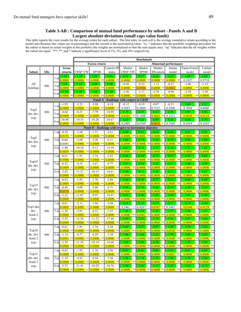
Do mutual fund managers have superior skills? 49
Table 3-AB : Comparison of mutual fund performance by subset - Panels A and B Largest absolute deviations (small caps value funds)
This table reports the t-test results for the average return for each subset. The first entry in each cell is the average cumulative return according to the model specification (the values are in percentage) and the second is the associated p-value. “wit “ indicates that the portfolio weighting procedure for the subset is based on actual weights in the portfolio (the weights are normalized so that the sum equals one). “eq” indicates that the all weights within the subset are equal. ***, **, and * indicate a significance level of 1%, 5%, and 10% respectively.
Subset Obs3.18 1.88 2.05 0.96 0.51 0.57 0.26 0.63 0.08 0.00
0.0000 *** 0.0000 *** 0.0000 *** 0.0000 *** 0.0000 *** 0.0000 *** 0.0000 *** 0.0000 *** 0.1927 0.97187.24 3.61 4.09 0.98 -0.48 -0.32 -1.12 -0.27 -1.06 -1.15
0.0000 *** 0.0000 *** 0.0000 *** 0.0000 *** 0.0008 *** 0.0506 * 0.0000 *** 0.0661 * 0.0000 *** 0.0000 ***15.30 6.48 7.60 1.14 -1.50 -1.17 -2.70 -0.96 -2.39 -3.36
0.0000 *** 0.0000 *** 0.0000 *** 0.0000 *** 0.0000 *** 0.0000 *** 0.0000 *** 0.0000 *** 0.0000 *** 0.0000 ***
-1.95 -3.25 -3.08 -4.18 -0.12 -0.19 -0.07 -0.21 0.08 0.110.0000 *** 0.0000 *** 0.0000 *** 0.0000 *** 0.5687 0.3809 0.7537 0.3200 0.7094 0.6060
806 -4.64 -8.27 -7.79 -10.89 0.75 0.53 0.93 0.56 0.91 0.820.0000 *** 0.0000 *** 0.0000 *** 0.0000 *** 0.0365 ** 0.1488 0.0065 *** 0.1212 0.0058 *** 0.0118 **-10.48 -19.33 -18.20 -24.67 0.67 0.24 0.95 0.20 0.64 0.750.0000 *** 0.0000 *** 0.0000 *** 0.0000 *** 0.2405 0.6769 0.0832 * 0.7305 0.2414 0.1635
1 m -0.38 -1.68 -1.51 -2.61 0.69 0.62 0.84 0.64 0.91 0.960.0193 ** 0.0000 *** 0.0000 *** 0.0000 *** 0.0000 *** 0.0001 *** 0.0000 *** 0.0000 *** 0.0000 *** 0.0000 ***
806 3 m -0.06 -3.69 -3.20 -6.31 2.84 2.72 3.13 2.78 2.95 3.000.8481 0.0000 *** 0.0000 *** 0.0000 *** 0.0000 *** 0.0000 *** 0.0000 *** 0.0000 *** 0.0000 *** 0.0000 ***
6 m -1.40 -10.24 -9.12 -15.59 4.57 4.24 5.27 4.38 4.71 5.020.0029 *** 0.0000 *** 0.0000 *** 0.0000 *** 0.0000 *** 0.0000 *** 0.0000 *** 0.0000 *** 0.0000 *** 0.0000 ***
1 m -0.61 -1.91 -1.74 -2.83 0.56 0.49 0.73 0.51 0.80 0.850.0000 *** 0.0000 *** 0.0000 *** 0.0000 *** 0.0000 *** 0.0000 *** 0.0000 *** 0.0000 *** 0.0000 *** 0.0000 ***
806 3 m -0.52 -4.15 -3.67 -6.77 2.75 2.59 3.23 2.67 2.94 2.990.0409 ** 0.0000 *** 0.0000 *** 0.0000 *** 0.0000 *** 0.0000 *** 0.0000 *** 0.0000 *** 0.0000 *** 0.0000 ***
6 m -2.42 -11.27 -10.15 -16.61 4.50 4.11 5.46 4.27 4.65 5.070.0000 *** 0.0000 *** 0.0000 *** 0.0000 *** 0.0000 *** 0.0000 *** 0.0000 *** 0.0000 *** 0.0000 *** 0.0000 ***
1 m -0.63 -1.93 -1.76 -2.86 0.58 0.50 0.77 0.52 0.84 0.880.0000 *** 0.0000 *** 0.0000 *** 0.0000 *** 0.0000 *** 0.0000 *** 0.0000 *** 0.0000 *** 0.0000 *** 0.0000 ***
806 3 m -0.46 -4.09 -3.60 -6.71 2.94 2.76 3.46 2.86 3.14 3.200.0510 * 0.0000 *** 0.0000 *** 0.0000 *** 0.0000 *** 0.0000 *** 0.0000 *** 0.0000 *** 0.0000 *** 0.0000 ***
6 m -2.22 -11.07 -9.95 -16.41 4.92 4.48 5.95 4.68 5.01 5.480.0000 *** 0.0000 *** 0.0000 *** 0.0000 *** 0.0000 *** 0.0000 *** 0.0000 *** 0.0000 *** 0.0000 *** 0.0000 ***
1 m -0.81 -2.11 -1.94 -3.04 0.21 0.14 0.37 0.17 0.39 0.440.0000 *** 0.0000 *** 0.0000 *** 0.0000 *** 0.2461 0.4287 0.0307 ** 0.3487 0.0248 ** 0.0118 **
806 3 m -1.38 -5.01 -4.52 -7.63 1.43 1.28 1.88 1.37 1.56 1.670.0004 *** 0.0000 *** 0.0000 *** 0.0000 *** 0.0000 *** 0.0001 *** 0.0000 *** 0.0000 *** 0.0000 *** 0.0000 ***
6 m -3.52 -12.34 -11.22 -17.69 2.59 2.22 3.38 2.41 2.51 3.040.0000 *** 0.0000 *** 0.0000 *** 0.0000 *** 0.0000 *** 0.0000 *** 0.0000 *** 0.0000 *** 0.0000 *** 0.0000 ***
1 m -0.61 -1.91 -1.74 -2.84 0.43 0.37 0.57 0.39 0.59 0.620.0000 *** 0.0000 *** 0.0000 *** 0.0000 *** 0.0009 *** 0.0051 *** 0.0000 *** 0.0028 *** 0.0000 *** 0.0000 ***
806 3 m -1.14 -4.77 -4.29 -7.39 1.80 1.64 2.23 1.75 1.92 2.020.0001 *** 0.0000 *** 0.0000 *** 0.0000 *** 0.0000 *** 0.0000 *** 0.0000 *** 0.0000 *** 0.0000 *** 0.0000 ***
6 m -2.39 -11.26 -10.14 -16.60 3.63 3.26 4.38 3.46 3.52 3.960.0000 *** 0.0000 *** 0.0000 *** 0.0000 *** 0.0000 *** 0.0000 *** 0.0000 *** 0.0000 *** 0.0000 *** 0.0000 ***
1 m -0.63 -1.93 -1.76 -2.86 0.47 0.41 0.60 0.43 0.61 0.650.0000 *** 0.0000 *** 0.0000 *** 0.0000 *** 0.0000 *** 0.0003 *** 0.0000 *** 0.0001 *** 0.0000 *** 0.0000 ***
806 3 m -1.19 -4.82 -4.34 -7.44 1.90 1.74 2.30 1.85 1.98 2.080.0000 *** 0.0000 *** 0.0000 *** 0.0000 *** 0.0000 *** 0.0000 *** 0.0000 *** 0.0000 *** 0.0000 *** 0.0000 ***
6 m -2.53 -11.41 -10.29 -16.76 3.80 3.42 4.53 3.62 3.65 4.120.0000 *** 0.0000 *** 0.0000 *** 0.0000 *** 0.0000 *** 0.0000 *** 0.0000 *** 0.0000 *** 0.0000 *** 0.0000 ***
Top15 abs. dev. Scale 2
(eq)
Top5 abs. dev.
Scale 2 (eq)
Panel B - Rankings with respect to investment objective
Top5 abs. dev.
(eq)
Top10 abs. dev. Scale 2
(eq)
Top10 abs. dev.
(eq)
Top15 abs. dev.
(eq)
Panel A - Rankings with respect to CRSP
Top5 abs. dev.
(eq)
1 m
3 m
6 m
Fama-French model
Carhart model
All holdings 806
1 m
3 m
6 m
Market CRSP-VW
Market SP500
Market SPcustom
Jensen model
Gross returns CRSP-VW SP500
Custom SP index
BenchmarkExcess return Abnormal performance

Do mutual fund managers have superior skills? 50
Table 4-AB : Comparison of mutual fund performance by subset - Panels A and B Largest positive deviations (all funds)
This table reports the t-test results for the average return for each subset. The first entry in each cell is the average cumulative return according to the model specification (the values are in percentage) and the second is the associated p-value. “wit “ indicates that the portfolio weighting procedure for the subset is based on actual weights in the portfolio (the weights are normalized so that the sum equals one). “eq” indicates that the all weights within the subset are equal. ***, **, and * indicate a significance level of 1%, 5%, and 10% respectively.
Subset Obs2.18 0.89 1.06 0.79 -0.75 -0.74 -0.57 -0.66 -0.89 -0.91
0.0000 *** 0.0000 *** 0.0000 *** 0.0000 *** 0.0000 *** 0.0000 *** 0.0000 *** 0.0000 *** 0.0000 *** 0.0000 ***4.77 1.18 1.65 0.71 -3.49 -3.50 -3.14 -3.38 -3.71 -3.75
0.0000 *** 0.0000 *** 0.0000 *** 0.0000 *** 0.0000 *** 0.0000 *** 0.0000 *** 0.0000 *** 0.0000 *** 0.0000 ***9.85 1.30 2.39 0.67 -7.34 -7.36 -6.46 -6.96 -7.78 -8.04
0.0000 *** 0.0000 *** 0.0000 *** 0.0000 *** 0.0000 *** 0.0000 *** 0.0000 *** 0.0000 *** 0.0000 *** 0.0000 ***
2.66 1.37 1.54 1.27 -0.66 -0.59 -0.42 -0.57 -0.86 -0.890.0000 *** 0.0000 *** 0.0000 *** 0.0000 *** 0.0000 *** 0.0000 *** 0.0000 *** 0.0000 *** 0.0000 *** 0.0000 ***
8385 6.02 2.43 2.90 1.96 -3.25 -3.12 -2.80 -3.16 -3.43 -3.500.0000 *** 0.0000 *** 0.0000 *** 0.0000 *** 0.0000 *** 0.0000 *** 0.0000 *** 0.0000 *** 0.0000 *** 0.0000 ***11.93 3.39 4.47 2.76 -7.37 -7.09 -6.27 -7.01 -7.48 -7.88
0.0000 *** 0.0000 *** 0.0000 *** 0.0000 *** 0.0000 *** 0.0000 *** 0.0000 *** 0.0000 *** 0.0000 *** 0.0000 ***
1 m 3.89 2.61 2.77 2.50 0.76 0.77 0.94 0.85 0.62 0.620.0000 *** 0.0000 *** 0.0000 *** 0.0000 *** 0.0000 *** 0.0000 *** 0.0000 *** 0.0000 *** 0.0000 *** 0.0000 ***
8385 3 m 6.28 2.70 3.17 2.23 -2.45 -2.47 -2.08 -2.35 -2.72 -2.740.0000 *** 0.0000 *** 0.0000 *** 0.0000 *** 0.0000 *** 0.0000 *** 0.0000 *** 0.0000 *** 0.0000 *** 0.0000 ***
6 m 11.22 2.69 3.77 2.05 -6.79 -6.86 -5.95 -6.44 -7.33 -7.580.0000 *** 0.0000 *** 0.0000 *** 0.0000 *** 0.0000 *** 0.0000 *** 0.0000 *** 0.0000 *** 0.0000 *** 0.0000 ***
1 m 2.21 0.93 1.09 0.82 -0.84 -0.82 -0.70 -0.74 -1.13 -1.150.0000 *** 0.0000 *** 0.0000 *** 0.0000 *** 0.0000 *** 0.0000 *** 0.0000 *** 0.0000 *** 0.0000 *** 0.0000 ***
8385 3 m 5.52 1.93 2.40 1.46 -3.22 -3.19 -2.98 -3.10 -3.73 -3.810.0000 *** 0.0000 *** 0.0000 *** 0.0000 *** 0.0000 *** 0.0000 *** 0.0000 *** 0.0000 *** 0.0000 *** 0.0000 ***
6 m 11.51 2.96 4.04 2.34 -6.79 -6.74 -6.16 -6.38 -7.71 -8.250.0000 *** 0.0000 *** 0.0000 *** 0.0000 *** 0.0000 *** 0.0000 *** 0.0000 *** 0.0000 *** 0.0000 *** 0.0000 ***
1 m 3.83 2.54 2.71 2.44 0.74 0.75 0.93 0.83 0.61 0.600.0000 *** 0.0000 *** 0.0000 *** 0.0000 *** 0.0000 *** 0.0000 *** 0.0000 *** 0.0000 *** 0.0000 *** 0.0000 ***
8385 3 m 6.08 2.50 2.97 2.03 -2.49 -2.51 -2.10 -2.38 -2.74 -2.790.0000 *** 0.0000 *** 0.0000 *** 0.0000 *** 0.0000 *** 0.0000 *** 0.0000 *** 0.0000 *** 0.0000 *** 0.0000 ***
6 m 11.02 2.48 3.56 1.85 -6.65 -6.73 -5.75 -6.28 -7.18 -7.490.0000 *** 0.0000 *** 0.0000 *** 0.0000 *** 0.0000 *** 0.0000 *** 0.0000 *** 0.0000 *** 0.0000 *** 0.0000 ***
1 m 2.70 1.42 1.59 1.32 -0.25 -0.24 -0.14 -0.15 -0.49 -0.490.0000 *** 0.0000 *** 0.0000 *** 0.0000 *** 0.0000 *** 0.0000 *** 0.0028 *** 0.0029 *** 0.0000 *** 0.0000 ***
8385 3 m 5.49 1.90 2.38 1.46 -2.95 -2.96 -2.77 -2.81 -3.37 -3.460.0000 *** 0.0000 *** 0.0000 *** 0.0000 *** 0.0000 *** 0.0000 *** 0.0000 *** 0.0000 *** 0.0000 *** 0.0000 ***
6 m 10.99 2.43 3.51 1.84 -6.69 -6.75 -6.19 -6.28 -7.54 -8.010.0000 *** 0.0000 *** 0.0000 *** 0.0000 *** 0.0000 *** 0.0000 *** 0.0000 *** 0.0000 *** 0.0000 *** 0.0000 ***
1 m 3.58 2.29 2.46 2.19 0.50 0.52 0.71 0.59 0.39 0.370.0000 *** 0.0000 *** 0.0000 *** 0.0000 *** 0.0000 *** 0.0000 *** 0.0000 *** 0.0000 *** 0.0000 *** 0.0000 ***
8385 3 m 5.71 2.12 2.59 1.66 -2.76 -2.77 -2.34 -2.66 -2.96 -3.020.0000 *** 0.0000 *** 0.0000 *** 0.0000 *** 0.0000 *** 0.0000 *** 0.0000 *** 0.0000 *** 0.0000 *** 0.0000 ***
6 m 10.65 2.11 3.19 1.48 -6.80 -6.85 -5.85 -6.44 -7.22 -7.610.0000 *** 0.0000 *** 0.0000 *** 0.0000 *** 0.0000 *** 0.0000 *** 0.0000 *** 0.0000 *** 0.0000 *** 0.0000 ***
BenchmarkExcess return Abnormal performance
Market SPcustom
Jensen model
Gross returns CRSP-VW SP500
Custom SP index
Fama-French model
Carhart model
Panel A - Rankings with respect to CRSP
All holdings 8385
1 m
3 m
6 m
Market CRSP-VW
Market SP500
Top5 rel. dev. Scale 1
1 m
3 m
6 m
Top5 rel. dev.
Scale 1 (Inter)
Panel B - Rankings with respect to investment objective
Top5 pos. dev.
Top5 pos. dev. (Ponly)
Top5 pos. dev.
(Inter)
Top5 pos. dev.
(All)
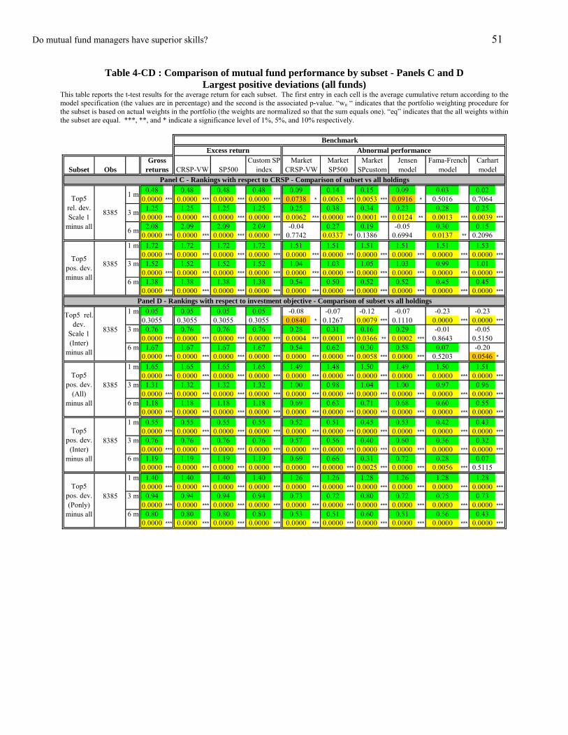
Do mutual fund managers have superior skills? 51
Table 4-CD : Comparison of mutual fund performance by subset - Panels C and D Largest positive deviations (all funds)
This table reports the t-test results for the average return for each subset. The first entry in each cell is the average cumulative return according to the model specification (the values are in percentage) and the second is the associated p-value. “wit “ indicates that the portfolio weighting procedure for the subset is based on actual weights in the portfolio (the weights are normalized so that the sum equals one). “eq” indicates that the all weights within the subset are equal. ***, **, and * indicate a significance level of 1%, 5%, and 10% respectively.
Subset Obs
0.48 0.48 0.48 0.48 0.09 0.14 0.15 0.09 0.03 0.020.0000 *** 0.0000 *** 0.0000 *** 0.0000 *** 0.0738 * 0.0063 *** 0.0053 *** 0.0916 * 0.5016 0.7064
1.25 1.25 1.25 1.25 0.25 0.38 0.34 0.23 0.28 0.250.0000 *** 0.0000 *** 0.0000 *** 0.0000 *** 0.0062 *** 0.0000 *** 0.0001 *** 0.0124 ** 0.0013 *** 0.0039 ***
2.08 2.09 2.09 2.09 -0.04 0.27 0.19 -0.05 0.30 0.150.0000 *** 0.0000 *** 0.0000 *** 0.0000 *** 0.7742 0.0337 ** 0.1386 0.6994 0.0137 ** 0.2096
1 m 1.72 1.72 1.72 1.72 1.51 1.51 1.51 1.51 1.51 1.530.0000 *** 0.0000 *** 0.0000 *** 0.0000 *** 0.0000 *** 0.0000 *** 0.0000 *** 0.0000 *** 0.0000 *** 0.0000 ***
8385 3 m 1.52 1.52 1.52 1.52 1.04 1.03 1.05 1.03 0.99 1.010.0000 *** 0.0000 *** 0.0000 *** 0.0000 *** 0.0000 *** 0.0000 *** 0.0000 *** 0.0000 *** 0.0000 *** 0.0000 ***
6 m 1.38 1.38 1.38 1.38 0.54 0.50 0.52 0.52 0.45 0.450.0000 *** 0.0000 *** 0.0000 *** 0.0000 *** 0.0000 *** 0.0000 *** 0.0000 *** 0.0000 *** 0.0000 *** 0.0000 ***
1 m 0.05 0.05 0.05 0.05 -0.08 -0.07 -0.12 -0.07 -0.23 -0.230.3055 0.3055 0.3055 0.3055 0.0840 * 0.1267 0.0079 *** 0.1110 0.0000 *** 0.0000 ***
8385 3 m 0.76 0.76 0.76 0.76 0.28 0.31 0.16 0.29 -0.01 -0.050.0000 *** 0.0000 *** 0.0000 *** 0.0000 *** 0.0004 *** 0.0001 *** 0.0366 ** 0.0002 *** 0.8643 0.5150
6 m 1.67 1.67 1.67 1.67 0.54 0.62 0.30 0.58 0.07 -0.200.0000 *** 0.0000 *** 0.0000 *** 0.0000 *** 0.0000 *** 0.0000 *** 0.0058 *** 0.0000 *** 0.5203 0.0546 *
1 m 1.65 1.65 1.65 1.65 1.49 1.48 1.50 1.49 1.50 1.510.0000 *** 0.0000 *** 0.0000 *** 0.0000 *** 0.0000 *** 0.0000 *** 0.0000 *** 0.0000 *** 0.0000 *** 0.0000 ***
8385 3 m 1.31 1.32 1.32 1.32 1.00 0.98 1.04 1.00 0.97 0.960.0000 *** 0.0000 *** 0.0000 *** 0.0000 *** 0.0000 *** 0.0000 *** 0.0000 *** 0.0000 *** 0.0000 *** 0.0000 ***
6 m 1.18 1.18 1.18 1.18 0.69 0.63 0.71 0.68 0.60 0.550.0000 *** 0.0000 *** 0.0000 *** 0.0000 *** 0.0000 *** 0.0000 *** 0.0000 *** 0.0000 *** 0.0000 *** 0.0000 ***
1 m 0.55 0.55 0.55 0.55 0.52 0.51 0.45 0.53 0.42 0.430.0000 *** 0.0000 *** 0.0000 *** 0.0000 *** 0.0000 *** 0.0000 *** 0.0000 *** 0.0000 *** 0.0000 *** 0.0000 ***
8385 3 m 0.76 0.76 0.76 0.76 0.57 0.56 0.40 0.60 0.36 0.320.0000 *** 0.0000 *** 0.0000 *** 0.0000 *** 0.0000 *** 0.0000 *** 0.0000 *** 0.0000 *** 0.0000 *** 0.0000 ***
6 m 1.19 1.19 1.19 1.19 0.69 0.66 0.31 0.72 0.28 0.070.0000 *** 0.0000 *** 0.0000 *** 0.0000 *** 0.0000 *** 0.0000 *** 0.0025 *** 0.0000 *** 0.0056 *** 0.5115
1 m 1.40 1.40 1.40 1.40 1.26 1.26 1.28 1.26 1.28 1.280.0000 *** 0.0000 *** 0.0000 *** 0.0000 *** 0.0000 *** 0.0000 *** 0.0000 *** 0.0000 *** 0.0000 *** 0.0000 ***
8385 3 m 0.94 0.94 0.94 0.94 0.73 0.72 0.80 0.72 0.75 0.730.0000 *** 0.0000 *** 0.0000 *** 0.0000 *** 0.0000 *** 0.0000 *** 0.0000 *** 0.0000 *** 0.0000 *** 0.0000 ***
6 m 0.80 0.80 0.80 0.80 0.53 0.51 0.60 0.51 0.56 0.430.0000 *** 0.0000 *** 0.0000 *** 0.0000 *** 0.0000 *** 0.0000 *** 0.0000 *** 0.0000 *** 0.0000 *** 0.0000 ***
Top5 pos. dev.
(All) minus all
Top5 pos. dev.
(Inter) minus all
Top5 pos. dev. (Ponly)
minus all
Top5 pos. dev. minus all
Panel D - Rankings with respect to investment objective - Comparison of subset vs all holdings
Top5 rel. dev.
Scale 1 (Inter)
minus all
Panel C - Rankings with respect to CRSP - Comparison of subset vs all holdings
Top5 rel. dev. Scale 1
minus all
8385
1 m
3 m
6 m
Fama-French model
Carhart model
Market CRSP-VW
Market SP500
Market SPcustom
Jensen model
Gross returns CRSP-VW SP500
Custom SP index
Excess return Abnormal performanceBenchmark

Do mutual fund managers have superior skills? 52
Table 5-AB : Comparison of mutual fund performance by subset - Panels A and B Largest positive deviations (small caps value funds)
This table reports the t-test results for the average return for each subset. The first entry in each cell is the average cumulative return according to the model specification (the values are in percentage) and the second is the associated p-value. “wit “ indicates that the portfolio weighting procedure for the subset is based on actual weights in the portfolio (the weights are normalized so that the sum equals one). “eq” indicates that the all weights within the subset are equal. ***, **, and * indicate a significance level of 1%, 5%, and 10% respectively.
Subset Obs3.18 1.88 2.05 0.96 0.51 0.57 0.26 0.63 0.08 0.00
0.0000 *** 0.0000 *** 0.0000 *** 0.0000 *** 0.0000 *** 0.0000 *** 0.0000 *** 0.0000 *** 0.1927 0.97187.24 3.61 4.09 0.98 -0.48 -0.32 -1.12 -0.27 -1.06 -1.15
0.0000 *** 0.0000 *** 0.0000 *** 0.0000 *** 0.0008 *** 0.0506 * 0.0000 *** 0.0661 * 0.0000 *** 0.0000 ***15.30 6.48 7.60 1.14 -1.50 -1.17 -2.70 -0.96 -2.39 -3.36
0.0000 *** 0.0000 *** 0.0000 *** 0.0000 *** 0.0000 *** 0.0000 *** 0.0000 *** 0.0000 *** 0.0000 *** 0.0000 ***
3.72 2.43 2.60 1.50 1.24 1.35 1.06 1.36 0.82 0.750.0000 *** 0.0000 *** 0.0000 *** 0.0000 *** 0.0000 *** 0.0000 *** 0.0000 *** 0.0000 *** 0.0001 *** 0.0003 ***
806 8.19 4.56 5.05 1.94 0.89 1.21 0.19 1.11 0.35 0.230.0000 *** 0.0000 *** 0.0000 *** 0.0000 *** 0.0204 ** 0.0026 *** 0.5969 0.0041 *** 0.3123 0.512016.68 7.82 8.95 2.48 0.31 1.01 -0.90 0.88 -0.11 -1.04
0.0000 *** 0.0000 *** 0.0000 *** 0.0001 *** 0.5941 0.0947 * 0.0839 * 0.1318 0.8230 0.0359 **
1 m 5.63 4.33 4.50 3.41 2.64 2.69 2.36 2.76 2.20 2.100.0000 *** 0.0000 *** 0.0000 *** 0.0000 *** 0.0000 *** 0.0000 *** 0.0000 *** 0.0000 *** 0.0000 *** 0.0000 ***
806 3 m 9.65 6.02 6.51 3.40 1.20 1.35 0.58 1.42 0.50 0.420.0000 *** 0.0000 *** 0.0000 *** 0.0000 *** 0.0000 *** 0.0000 *** 0.0294 ** 0.0000 *** 0.0542 * 0.1064
6 m 17.94 9.10 10.22 3.76 -0.27 0.01 -1.51 0.28 -1.39 -2.460.0000 *** 0.0000 *** 0.0000 *** 0.0000 *** 0.5364 0.9745 0.0001 *** 0.5219 0.0004 *** 0.0000 ***
1 m 3.00 1.71 1.88 0.78 0.35 0.47 -0.02 0.48 -0.10 -0.180.0000 *** 0.0000 *** 0.0000 *** 0.0001 *** 0.1077 0.0370 ** 0.9081 0.0304 ** 0.6323 0.3838
806 3 m 6.20 2.60 3.08 -0.02 -1.46 -1.16 -2.46 -1.26 -1.95 -2.150.0000 *** 0.0000 *** 0.0000 *** 0.9601 0.0002 *** 0.0045 *** 0.0000 *** 0.0015 *** 0.0000 *** 0.0000 ***
6 m 12.32 3.54 4.66 -1.80 -4.37 -3.72 -6.24 -3.81 -4.80 -6.120.0000 *** 0.0000 *** 0.0000 *** 0.0022 *** 0.0000 *** 0.0000 *** 0.0000 *** 0.0000 *** 0.0000 *** 0.0000 ***
1 m 5.64 4.34 4.51 3.41 2.65 2.70 2.38 2.77 2.22 2.120.0000 *** 0.0000 *** 0.0000 *** 0.0000 *** 0.0000 *** 0.0000 *** 0.0000 *** 0.0000 *** 0.0000 *** 0.0000 ***
806 3 m 9.71 6.08 6.57 3.46 1.27 1.42 0.67 1.49 0.57 0.500.0000 *** 0.0000 *** 0.0000 *** 0.0000 *** 0.0000 *** 0.0000 *** 0.0120 ** 0.0000 *** 0.0304 ** 0.0555 *
6 m 18.18 9.36 10.48 4.02 0.00 0.27 -1.19 0.55 -1.15 -2.190.0000 *** 0.0000 *** 0.0000 *** 0.0000 *** 0.9961 0.5432 0.0021 *** 0.2145 0.0038 *** 0.0000 ***
1 m 3.28 2.00 2.17 1.06 0.58 0.69 0.20 0.71 0.13 0.050.0000 *** 0.0000 *** 0.0000 *** 0.0000 *** 0.0079 *** 0.0019 *** 0.3246 0.0013 *** 0.5260 0.7888
806 3 m 6.12 2.55 3.04 -0.07 -1.68 -1.41 -2.63 -1.47 -2.10 -2.270.0000 *** 0.0000 *** 0.0000 *** 0.8608 0.0000 *** 0.0004 *** 0.0000 *** 0.0001 *** 0.0000 *** 0.0000 ***
6 m 12.28 3.52 4.64 -1.83 -4.68 -4.09 -6.48 -4.12 -5.03 -6.350.0000 *** 0.0000 *** 0.0000 *** 0.0015 *** 0.0000 *** 0.0000 *** 0.0000 *** 0.0000 *** 0.0000 *** 0.0000 ***
1 m 5.55 4.25 4.42 3.33 2.56 2.61 2.32 2.68 2.13 2.040.0000 *** 0.0000 *** 0.0000 *** 0.0000 *** 0.0000 *** 0.0000 *** 0.0000 *** 0.0000 *** 0.0000 *** 0.0000 ***
806 3 m 9.60 5.97 6.46 3.35 1.15 1.29 0.57 1.37 0.45 0.370.0000 *** 0.0000 *** 0.0000 *** 0.0000 *** 0.0001 *** 0.0000 *** 0.0347 ** 0.0000 *** 0.0913 * 0.1617
6 m 18.40 9.57 10.70 4.23 0.17 0.43 -0.99 0.72 -0.99 -2.030.0000 *** 0.0000 *** 0.0000 *** 0.0000 *** 0.6915 0.3417 0.0112 ** 0.1020 0.0122 ** 0.0000 ***
BenchmarkExcess return Abnormal performance
Market SPcustom
Jensen model
Gross returns CRSP-VW SP500
Custom SP index
Fama-French model
Carhart model
Panel A - Rankings with respect to CRSP
All holdings 806
1 m
3 m
6 m
Market CRSP-VW
Market SP500
Top5 rel. dev. Scale 1
1 m
3 m
6 m
Top5 rel. dev.
Scale 1 (Inter)
Panel B - Rankings with respect to investment objective
Top5 pos. dev.
Top5 pos. dev. (Ponly)
Top5 pos. dev.
(Inter)
Top5 pos. dev.
(All)

Do mutual fund managers have superior skills? 53
Table 5-CD : Comparison of mutual fund performance by subset - Panels C and D Largest positive deviations (small caps value funds)
This table reports the t-test results for the average return for each subset. The first entry in each cell is the average cumulative return according to the model specification (the values are in percentage) and the second is the associated p-value. “wit “ indicates that the portfolio weighting procedure for the subset is based on actual weights in the portfolio (the weights are normalized so that the sum equals one). “eq” indicates that the all weights within the subset are equal. ***, **, and * indicate a significance level of 1%, 5%, and 10% respectively.
Subset Obs
0.54 0.54 0.54 0.54 0.73 0.77 0.80 0.73 0.74 0.740.0047 *** 0.0047 *** 0.0047 *** 0.0047 *** 0.0001 *** 0.0001 *** 0.0000 *** 0.0001 *** 0.0001 *** 0.0001 ***
0.96 0.96 0.96 0.96 1.37 1.53 1.31 1.38 1.41 1.380.0069 *** 0.0069 *** 0.0069 *** 0.0069 *** 0.0000 *** 0.0000 *** 0.0000 *** 0.0000 *** 0.0000 *** 0.0000 ***
1.38 1.34 1.34 1.34 1.81 2.18 1.80 1.84 2.28 2.310.0139 ** 0.0166 ** 0.0166 ** 0.0166 ** 0.0002 *** 0.0000 *** 0.0001 *** 0.0002 *** 0.0000 *** 0.0000 ***
1 m 2.45 2.45 2.45 2.45 2.13 2.12 2.09 2.13 2.12 2.090.0000 *** 0.0000 *** 0.0000 *** 0.0000 *** 0.0000 *** 0.0000 *** 0.0000 *** 0.0000 *** 0.0000 *** 0.0000 ***
806 3 m 2.41 2.41 2.41 2.41 1.68 1.67 1.70 1.68 1.56 1.570.0000 *** 0.0000 *** 0.0000 *** 0.0000 *** 0.0000 *** 0.0000 *** 0.0000 *** 0.0000 *** 0.0000 *** 0.0000 ***
6 m 2.64 2.62 2.62 2.62 1.23 1.18 1.19 1.24 1.00 0.900.0000 *** 0.0000 *** 0.0000 *** 0.0000 *** 0.0002 *** 0.0004 *** 0.0001 *** 0.0002 *** 0.0016 *** 0.0035 ***
1 m -0.16 -0.16 -0.16 -0.16 -0.15 -0.10 -0.27 -0.14 -0.17 -0.170.4083 0.4083 0.4083 0.4083 0.4433 0.6070 0.1572 0.4576 0.3722 0.3710
806 3 m -1.00 -1.00 -1.00 -1.00 -1.00 -0.86 -1.35 -1.01 -0.92 -1.020.0049 *** 0.0049 *** 0.0049 *** 0.0049 *** 0.0034 *** 0.0121 ** 0.0000 *** 0.0032 *** 0.0053 *** 0.0015 ***
6 m -2.95 -2.93 -2.93 -2.93 -2.92 -2.61 -3.59 -2.91 -2.48 -2.820.0000 *** 0.0000 *** 0.0000 *** 0.0000 *** 0.0000 *** 0.0000 *** 0.0000 *** 0.0000 *** 0.0000 *** 0.0000 ***
1 m 2.46 2.46 2.46 2.46 2.14 2.13 2.12 2.14 2.14 2.120.0000 *** 0.0000 *** 0.0000 *** 0.0000 *** 0.0000 *** 0.0000 *** 0.0000 *** 0.0000 *** 0.0000 *** 0.0000 ***
806 3 m 2.47 2.47 2.47 2.47 1.75 1.74 1.79 1.76 1.63 1.650.0000 *** 0.0000 *** 0.0000 *** 0.0000 *** 0.0000 *** 0.0000 *** 0.0000 *** 0.0000 *** 0.0000 *** 0.0000 ***
6 m 2.89 2.88 2.88 2.88 1.50 1.44 1.51 1.51 1.24 1.170.0000 *** 0.0000 *** 0.0000 *** 0.0000 *** 0.0000 *** 0.0000 *** 0.0000 *** 0.0000 *** 0.0002 *** 0.0003 ***
1 m 0.16 0.16 0.16 0.16 0.10 0.15 -0.03 0.11 0.08 0.080.3982 0.3982 0.3982 0.3982 0.6019 0.4470 0.8825 0.5784 0.6711 0.6814
806 3 m -0.98 -0.98 -0.98 -0.98 -1.17 -1.05 -1.48 -1.17 -1.03 -1.110.0043 *** 0.0043 *** 0.0043 *** 0.0043 *** 0.0004 *** 0.0015 *** 0.0000 *** 0.0004 *** 0.0013 *** 0.0004 ***
6 m -2.87 -2.86 -2.86 -2.86 -3.16 -2.91 -3.75 -3.15 -2.66 -3.000.0000 *** 0.0000 *** 0.0000 *** 0.0000 *** 0.0000 *** 0.0000 *** 0.0000 *** 0.0000 *** 0.0000 *** 0.0000 ***
1 m 2.37 2.37 2.37 2.37 2.05 2.04 2.05 2.05 2.06 2.040.0000 *** 0.0000 *** 0.0000 *** 0.0000 *** 0.0000 *** 0.0000 *** 0.0000 *** 0.0000 *** 0.0000 *** 0.0000 ***
806 3 m 2.37 2.37 2.37 2.37 1.63 1.61 1.69 1.63 1.51 1.520.0000 *** 0.0000 *** 0.0000 *** 0.0000 *** 0.0000 *** 0.0000 *** 0.0000 *** 0.0000 *** 0.0000 *** 0.0000 ***
6 m 3.10 3.09 3.09 3.09 1.67 1.60 1.72 1.68 1.40 1.320.0000 *** 0.0000 *** 0.0000 *** 0.0000 *** 0.0000 *** 0.0000 *** 0.0000 *** 0.0000 *** 0.0000 *** 0.0000 ***
Top5 pos. dev.
(All) minus all
Top5 pos. dev.
(Inter) minus all
Top5 pos. dev. (Ponly)
minus all
Top5 pos. dev. minus all
Panel D - Rankings with respect to investment objective - Comparison of subset vs all holdings
Top5 rel. dev.
Scale 1 (Inter)
minus all
Panel C - Rankings with respect to CRSP - Comparison of subset vs all holdings
Top5 rel. dev. Scale 1
minus all
806
1 m
3 m
6 m
Fama-French model
Carhart model
Market CRSP-VW
Market SP500
Market SPcustom
Jensen model
Gross returns CRSP-VW SP500
Custom SP index
Excess return Abnormal performanceBenchmark
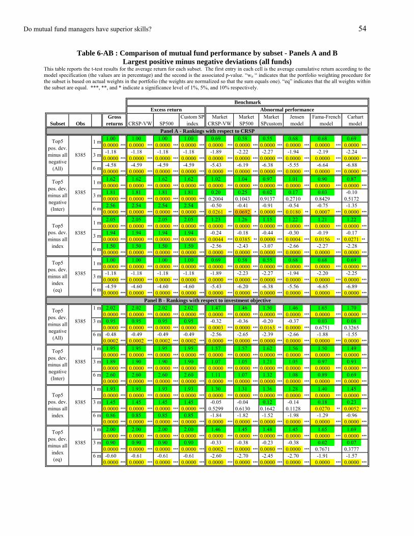
Do mutual fund managers have superior skills? 54
Table 6-AB : Comparison of mutual fund performance by subset - Panels A and B Largest positive minus negative deviations (all funds)
This table reports the t-test results for the average return for each subset. The first entry in each cell is the average cumulative return according to the model specification (the values are in percentage) and the second is the associated p-value. “wit “ indicates that the portfolio weighting procedure for the subset is based on actual weights in the portfolio (the weights are normalized so that the sum equals one). “eq” indicates that the all weights within the subset are equal. ***, **, and * indicate a significance level of 1%, 5%, and 10% respectively.
Subset Obs
1.00 1.00 1.00 1.00 0.69 0.58 0.55 0.68 0.68 0.690.0000 *** 0.0000 *** 0.0000 *** 0.0000 *** 0.0000 *** 0.0000 *** 0.0000 *** 0.0000 *** 0.0000 *** 0.0000 ***-1.18 -1.18 -1.18 -1.18 -1.89 -2.22 -2.27 -1.94 -2.19 -2.24
0.0000 *** 0.0000 *** 0.0000 *** 0.0000 *** 0.0000 *** 0.0000 *** 0.0000 *** 0.0000 *** 0.0000 *** 0.0000 ***-4.58 -4.59 -4.59 -4.59 -5.43 -6.19 -6.38 -5.55 -6.64 -6.88
0.0000 *** 0.0000 *** 0.0000 *** 0.0000 *** 0.0000 *** 0.0000 *** 0.0000 *** 0.0000 *** 0.0000 *** 0.0000 ***
1.62 1.62 1.62 1.62 1.02 1.04 0.97 1.01 0.90 0.870.0000 *** 0.0000 *** 0.0000 *** 0.0000 *** 0.0000 *** 0.0000 *** 0.0000 *** 0.0000 *** 0.0000 *** 0.0000 ***
8385 1.81 1.81 1.81 1.81 0.20 0.25 0.02 0.17 0.03 -0.100.0000 *** 0.0000 *** 0.0000 *** 0.0000 *** 0.2004 0.1043 0.9137 0.2710 0.8429 0.5172
2.56 2.54 2.54 2.54 -0.50 -0.41 -0.91 -0.54 -0.75 -1.350.0000 *** 0.0000 *** 0.0000 *** 0.0000 *** 0.0261 ** 0.0692 * 0.0000 *** 0.0180 ** 0.0007 *** 0.0000 ***
2.05 2.05 2.05 2.05 1.23 1.26 1.15 1.22 1.21 1.220.0000 *** 0.0000 *** 0.0000 *** 0.0000 *** 0.0000 *** 0.0000 *** 0.0000 *** 0.0000 *** 0.0000 *** 0.0000 ***
8385 1.94 1.94 1.94 1.94 -0.24 -0.18 -0.44 -0.30 -0.19 -0.170.0000 *** 0.0000 *** 0.0000 *** 0.0000 *** 0.0044 *** 0.0385 ** 0.0000 *** 0.0004 *** 0.0156 ** 0.0271 **
1.50 1.50 1.50 1.50 -2.56 -2.43 -3.07 -2.66 -2.27 -2.280.0000 *** 0.0000 *** 0.0000 *** 0.0000 *** 0.0000 *** 0.0000 *** 0.0000 *** 0.0000 *** 0.0000 *** 0.0000 ***
1.00 1.00 1.00 1.00 0.69 0.58 0.55 0.68 0.68 0.690.0000 *** 0.0000 *** 0.0000 *** 0.0000 *** 0.0000 *** 0.0000 *** 0.0000 *** 0.0000 *** 0.0000 *** 0.0000 ***
8385 -1.18 -1.18 -1.18 -1.18 -1.89 -2.23 -2.27 -1.94 -2.20 -2.250.0000 *** 0.0000 *** 0.0000 *** 0.0000 *** 0.0000 *** 0.0000 *** 0.0000 *** 0.0000 *** 0.0000 *** 0.0000 ***-4.59 -4.60 -4.60 -4.60 -5.43 -6.20 -6.38 -5.56 -6.65 -6.89
0.0000 *** 0.0000 *** 0.0000 *** 0.0000 *** 0.0000 *** 0.0000 *** 0.0000 *** 0.0000 *** 0.0000 *** 0.0000 ***
1 m 2.02 2.02 2.02 2.02 1.47 1.46 1.50 1.46 1.65 1.700.0000 *** 0.0000 *** 0.0000 *** 0.0000 *** 0.0000 *** 0.0000 *** 0.0000 *** 0.0000 *** 0.0000 *** 0.0000 ***
8385 3 m 0.95 0.95 0.95 0.95 -0.32 -0.36 -0.20 -0.37 0.03 0.080.0000 *** 0.0000 *** 0.0000 *** 0.0000 *** 0.0003 *** 0.0000 *** 0.0163 ** 0.0000 *** 0.6751 0.3265
6 m -0.48 -0.49 -0.49 -0.49 -2.56 -2.65 -2.39 -2.66 -1.88 -1.550.0002 *** 0.0002 *** 0.0002 *** 0.0002 *** 0.0000 *** 0.0000 *** 0.0000 *** 0.0000 *** 0.0000 *** 0.0000 ***
1 m 1.95 1.95 1.95 1.95 1.57 1.57 1.62 1.56 1.50 1.490.0000 *** 0.0000 *** 0.0000 *** 0.0000 *** 0.0000 *** 0.0000 *** 0.0000 *** 0.0000 *** 0.0000 *** 0.0000 ***
8385 3 m 1.89 1.90 1.90 1.90 1.07 1.05 1.21 1.05 0.97 0.930.0000 *** 0.0000 *** 0.0000 *** 0.0000 *** 0.0000 *** 0.0000 *** 0.0000 *** 0.0000 *** 0.0000 *** 0.0000 ***
6 m 2.60 2.60 2.60 2.60 1.11 1.07 1.32 1.08 0.89 0.690.0000 *** 0.0000 *** 0.0000 *** 0.0000 *** 0.0000 *** 0.0000 *** 0.0000 *** 0.0000 *** 0.0000 *** 0.0000 ***
1 m 1.93 1.93 1.93 1.93 1.30 1.31 1.36 1.28 1.40 1.450.0000 *** 0.0000 *** 0.0000 *** 0.0000 *** 0.0000 *** 0.0000 *** 0.0000 *** 0.0000 *** 0.0000 *** 0.0000 ***
8385 3 m 1.45 1.45 1.45 1.45 -0.05 -0.04 0.12 -0.14 0.18 0.230.0000 *** 0.0000 *** 0.0000 *** 0.0000 *** 0.5299 0.6130 0.1642 0.1128 0.0270 ** 0.0052 ***
6 m 0.86 0.85 0.85 0.85 -1.84 -1.82 -1.52 -1.98 -1.29 -0.960.0000 *** 0.0000 *** 0.0000 *** 0.0000 *** 0.0000 *** 0.0000 *** 0.0000 *** 0.0000 *** 0.0000 *** 0.0000 ***
1 m 2.00 2.00 2.00 2.00 1.46 1.45 1.48 1.45 1.65 1.690.0000 *** 0.0000 *** 0.0000 *** 0.0000 *** 0.0000 *** 0.0000 *** 0.0000 *** 0.0000 *** 0.0000 *** 0.0000 ***
8385 3 m 0.90 0.90 0.90 0.90 -0.33 -0.38 -0.23 -0.38 0.02 0.070.0000 *** 0.0000 *** 0.0000 *** 0.0000 *** 0.0002 *** 0.0000 *** 0.0080 *** 0.0000 *** 0.7671 0.3777
6 m -0.60 -0.61 -0.61 -0.61 -2.60 -2.70 -2.45 -2.70 -1.91 -1.570.0000 *** 0.0000 *** 0.0000 *** 0.0000 *** 0.0000 *** 0.0000 *** 0.0000 *** 0.0000 *** 0.0000 *** 0.0000 ***
Excess return Abnormal performanceBenchmark
Gross returns CRSP-VW SP500
Custom SP index
Fama-French model
Carhart model
Market CRSP-VW
Market SP500
Market SPcustom
Jensen model
Panel A - Rankings with respect to CRSP
Top5 pos. dev. minus all negative
(All)
8385
1 m
3 m
6 m
Top5 pos. dev. minus all negative (Inter)
1 m
3 m
6 m
Top5 pos. dev. minus all
index
1 m
3 m
6 m
3 m
6 m
Top5 pos. dev. minus all
index (eq)
1 m
Top5 pos. dev. minus all
index (eq)
Top5 pos. dev. minus all negative (Inter)
Top5 pos. dev. minus all
index
Panel B - Rankings with respect to investment objective
Top5 pos. dev. minus all negative
(All)

Do mutual fund managers have superior skills? 55
Table 7-AB : Comparison of mutual fund performance by subset - Panels A and B Largest positive minus negative deviations (small caps value funds)
This table reports the t-test results for the average return for each subset. The first entry in each cell is the average cumulative return according to the model specification (the values are in percentage) and the second is the associated p-value. “wit “ indicates that the portfolio weighting procedure for the subset is based on actual weights in the portfolio (the weights are normalized so that the sum equals one). “eq” indicates that the all weights within the subset are equal. ***, **, and * indicate a significance level of 1%, 5%, and 10% respectively.
Subset Obs
2.69 2.69 2.69 2.69 2.54 2.47 2.14 2.55 2.27 2.180.0000 *** 0.0000 *** 0.0000 *** 0.0000 *** 0.0000 *** 0.0000 *** 0.0000 *** 0.0000 *** 0.0000 *** 0.0000 ***
2.04 2.04 2.04 2.04 1.69 1.50 0.84 1.75 1.00 0.880.0000 *** 0.0000 *** 0.0000 *** 0.0000 *** 0.0000 *** 0.0000 *** 0.0035 *** 0.0000 *** 0.0002 *** 0.0016 ***
1.63 1.59 1.59 1.59 0.94 0.48 -1.01 1.00 -0.77 -1.840.0005 *** 0.0006 *** 0.0006 *** 0.0006 *** 0.0268 ** 0.2549 0.0156 ** 0.0191 ** 0.0527 * 0.0000 ***
2.65 2.65 2.65 2.65 2.00 2.03 1.82 2.00 2.04 2.100.0016 *** 0.0016 *** 0.0016 *** 0.0016 *** 0.0174 ** 0.0144 ** 0.0229 ** 0.0174 ** 0.0095 *** 0.0056 ***
806 2.86 2.86 2.86 2.86 1.11 1.10 0.51 1.08 0.85 0.580.0524 * 0.0524 * 0.0524 * 0.0524 * 0.3879 0.3915 0.6938 0.4071 0.4900 0.6627
5.85 5.82 5.82 5.82 2.23 2.24 1.30 2.21 1.91 1.260.0081 *** 0.0090 *** 0.0090 *** 0.0090 *** 0.2388 0.2304 0.4934 0.2495 0.2799 0.5054
3.86 3.86 3.86 3.86 3.14 3.22 2.73 3.15 2.80 2.710.0000 *** 0.0000 *** 0.0000 *** 0.0000 *** 0.0000 *** 0.0000 *** 0.0000 *** 0.0000 *** 0.0000 *** 0.0000 ***
806 5.54 5.54 5.54 5.54 3.53 3.77 2.60 3.58 3.12 3.070.0000 *** 0.0000 *** 0.0000 *** 0.0000 *** 0.0000 *** 0.0000 *** 0.0000 *** 0.0000 *** 0.0000 *** 0.0000 ***
8.53 8.51 8.51 8.51 4.22 4.74 2.10 4.32 3.91 3.010.0000 *** 0.0000 *** 0.0000 *** 0.0000 *** 0.0000 *** 0.0000 *** 0.0000 *** 0.0000 *** 0.0000 *** 0.0000 ***
2.69 2.69 2.69 2.69 2.54 2.47 2.14 2.55 2.27 2.180.0000 *** 0.0000 *** 0.0000 *** 0.0000 *** 0.0000 *** 0.0000 *** 0.0000 *** 0.0000 *** 0.0000 *** 0.0000 ***
806 2.04 2.04 2.04 2.04 1.69 1.50 0.84 1.75 1.00 0.880.0000 *** 0.0000 *** 0.0000 *** 0.0000 *** 0.0000 *** 0.0000 *** 0.0035 *** 0.0000 *** 0.0002 *** 0.0016 ***
1.62 1.59 1.59 1.59 0.94 0.48 -1.01 1.00 -0.78 -1.840.0005 *** 0.0007 *** 0.0007 *** 0.0007 *** 0.0269 ** 0.2554 0.0156 ** 0.0192 ** 0.0525 * 0.0000 ***
1 m 3.54 3.54 3.54 3.54 3.43 3.35 3.46 3.43 3.36 3.340.0000 *** 0.0000 *** 0.0000 *** 0.0000 *** 0.0000 *** 0.0000 *** 0.0000 *** 0.0000 *** 0.0000 *** 0.0000 ***
806 3 m 5.15 5.15 5.15 5.15 4.81 4.66 4.98 4.87 4.34 4.410.0000 *** 0.0000 *** 0.0000 *** 0.0000 *** 0.0000 *** 0.0000 *** 0.0000 *** 0.0000 *** 0.0000 *** 0.0000 ***
6 m 8.16 8.14 8.14 8.14 7.04 6.64 7.29 7.09 5.79 5.760.0000 *** 0.0000 *** 0.0000 *** 0.0000 *** 0.0000 *** 0.0000 *** 0.0000 *** 0.0000 *** 0.0000 *** 0.0000 ***
1 m 3.13 3.13 3.13 3.13 2.86 2.84 2.88 2.86 2.77 2.780.0000 *** 0.0000 *** 0.0000 *** 0.0000 *** 0.0000 *** 0.0000 *** 0.0000 *** 0.0000 *** 0.0000 *** 0.0000 ***
806 3 m 4.34 4.34 4.34 4.34 3.53 3.43 3.68 3.52 3.19 3.220.0000 *** 0.0000 *** 0.0000 *** 0.0000 *** 0.0000 *** 0.0000 *** 0.0000 *** 0.0000 *** 0.0000 *** 0.0000 ***
6 m 7.37 7.40 7.40 7.40 5.64 5.47 5.87 5.65 4.84 4.940.0000 *** 0.0000 *** 0.0000 *** 0.0000 *** 0.0000 *** 0.0000 *** 0.0000 *** 0.0000 *** 0.0000 *** 0.0000 ***
1 m 3.33 3.33 3.33 3.33 3.34 3.29 3.39 3.34 3.26 3.260.0000 *** 0.0000 *** 0.0000 *** 0.0000 *** 0.0000 *** 0.0000 *** 0.0000 *** 0.0000 *** 0.0000 *** 0.0000 ***
806 3 m 5.53 5.53 5.53 5.53 5.47 5.37 5.61 5.51 4.95 5.030.0000 *** 0.0000 *** 0.0000 *** 0.0000 *** 0.0000 *** 0.0000 *** 0.0000 *** 0.0000 *** 0.0000 *** 0.0000 ***
6 m 9.33 9.32 9.32 9.32 8.65 8.40 8.87 8.69 7.42 7.500.0000 *** 0.0000 *** 0.0000 *** 0.0000 *** 0.0000 *** 0.0000 *** 0.0000 *** 0.0000 *** 0.0000 *** 0.0000 ***
1 m 3.54 3.54 3.54 3.54 3.48 3.40 3.51 3.48 3.40 3.390.0000 *** 0.0000 *** 0.0000 *** 0.0000 *** 0.0000 *** 0.0000 *** 0.0000 *** 0.0000 *** 0.0000 *** 0.0000 ***
806 3 m 5.19 5.19 5.19 5.19 4.97 4.81 5.13 5.03 4.47 4.550.0000 *** 0.0000 *** 0.0000 *** 0.0000 *** 0.0000 *** 0.0000 *** 0.0000 *** 0.0000 *** 0.0000 *** 0.0000 ***
6 m 8.23 8.21 8.21 8.21 7.34 6.92 7.57 7.38 6.04 6.010.0000 *** 0.0000 *** 0.0000 *** 0.0000 *** 0.0000 *** 0.0000 *** 0.0000 *** 0.0000 *** 0.0000 *** 0.0000 ***
Excess return Abnormal performanceBenchmark
Gross returns CRSP-VW SP500
Custom SP index
Fama-French model
Carhart model
Market CRSP-VW
Market SP500
Market SPcustom
Jensen model
Panel A - Rankings with respect to CRSP
Top5 pos. dev. minus all negative
(All)
806
1 m
3 m
6 m
Top5 pos. dev. minus all negative (Inter)
1 m
3 m
6 m
Top5 pos. dev. minus all
index
1 m
3 m
6 m
3 m
6 m
Top5 pos. dev. minus all
index (eq)
1 m
Top5 pos. dev. minus all
index (eq)
Top5 pos. dev. minus all negative (Inter)
Top5 pos. dev. minus all
index
Panel B - Rankings with respect to investment objective
Top5 pos. dev. minus all negative
(All)
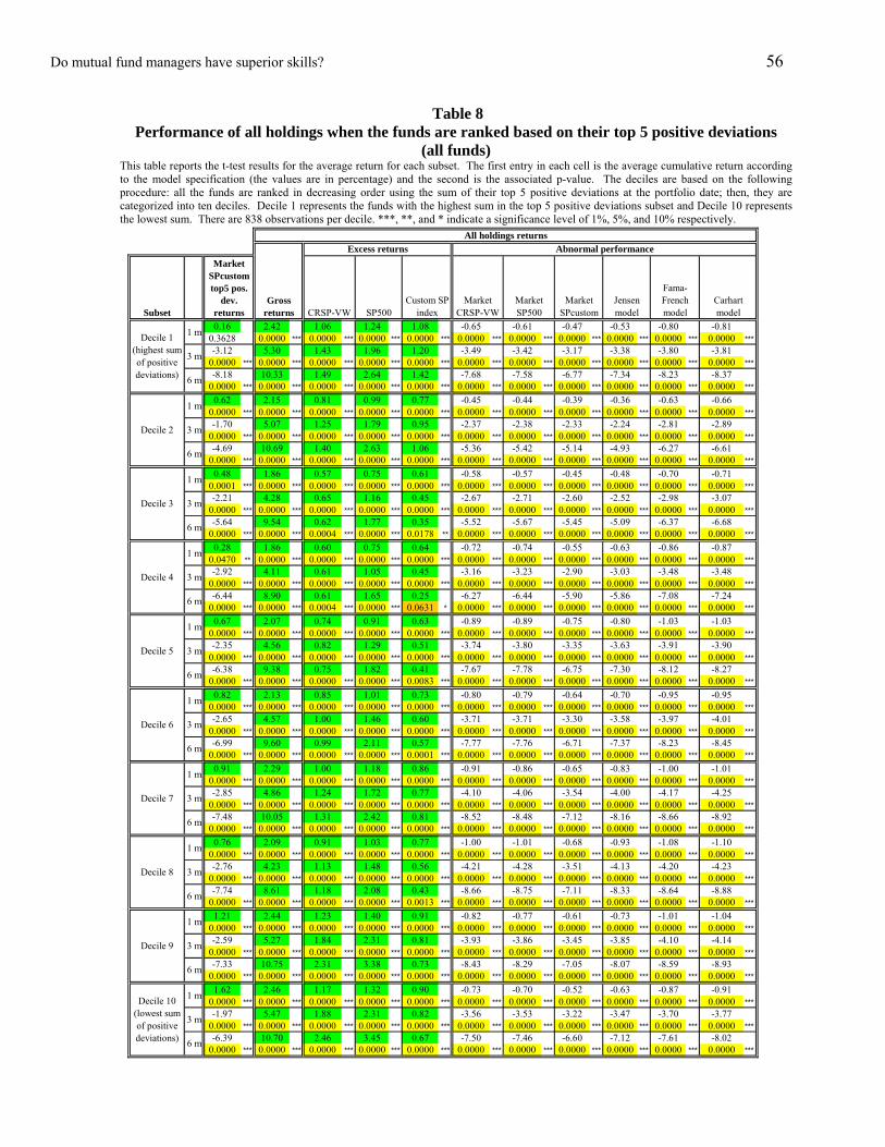
Do mutual fund managers have superior skills? 56
Table 8 Performance of all holdings when the funds are ranked based on their top 5 positive deviations
(all funds) This table reports the t-test results for the average return for each subset. The first entry in each cell is the average cumulative return according to the model specification (the values are in percentage) and the second is the associated p-value. The deciles are based on the following procedure: all the funds are ranked in decreasing order using the sum of their top 5 positive deviations at the portfolio date; then, they are categorized into ten deciles. Decile 1 represents the funds with the highest sum in the top 5 positive deviations subset and Decile 10 represents the lowest sum. There are 838 observations per decile. ***, **, and * indicate a significance level of 1%, 5%, and 10% respectively.
Subset0.16 2.42 1.06 1.24 1.08 -0.65 -0.61 -0.47 -0.53 -0.80 -0.81
0.3628 0.0000 *** 0.0000 *** 0.0000 *** 0.0000 *** 0.0000 *** 0.0000 *** 0.0000 *** 0.0000 *** 0.0000 *** 0.0000 ***-3.12 5.30 1.43 1.96 1.20 -3.49 -3.42 -3.17 -3.38 -3.80 -3.81
0.0000 *** 0.0000 *** 0.0000 *** 0.0000 *** 0.0000 *** 0.0000 *** 0.0000 *** 0.0000 *** 0.0000 *** 0.0000 *** 0.0000 ***-8.18 10.33 1.49 2.64 1.42 -7.68 -7.58 -6.77 -7.34 -8.23 -8.37
0.0000 *** 0.0000 *** 0.0000 *** 0.0000 *** 0.0000 *** 0.0000 *** 0.0000 *** 0.0000 *** 0.0000 *** 0.0000 *** 0.0000 ***
0.62 2.15 0.81 0.99 0.77 -0.45 -0.44 -0.39 -0.36 -0.63 -0.660.0000 *** 0.0000 *** 0.0000 *** 0.0000 *** 0.0000 *** 0.0000 *** 0.0000 *** 0.0000 *** 0.0000 *** 0.0000 *** 0.0000 ***-1.70 5.07 1.25 1.79 0.95 -2.37 -2.38 -2.33 -2.24 -2.81 -2.89
0.0000 *** 0.0000 *** 0.0000 *** 0.0000 *** 0.0000 *** 0.0000 *** 0.0000 *** 0.0000 *** 0.0000 *** 0.0000 *** 0.0000 ***-4.69 10.69 1.40 2.63 1.06 -5.36 -5.42 -5.14 -4.93 -6.27 -6.61
0.0000 *** 0.0000 *** 0.0000 *** 0.0000 *** 0.0000 *** 0.0000 *** 0.0000 *** 0.0000 *** 0.0000 *** 0.0000 *** 0.0000 ***
0.48 1.86 0.57 0.75 0.61 -0.58 -0.57 -0.45 -0.48 -0.70 -0.710.0001 *** 0.0000 *** 0.0000 *** 0.0000 *** 0.0000 *** 0.0000 *** 0.0000 *** 0.0000 *** 0.0000 *** 0.0000 *** 0.0000 ***-2.21 4.28 0.65 1.16 0.45 -2.67 -2.71 -2.60 -2.52 -2.98 -3.07
0.0000 *** 0.0000 *** 0.0000 *** 0.0000 *** 0.0000 *** 0.0000 *** 0.0000 *** 0.0000 *** 0.0000 *** 0.0000 *** 0.0000 ***-5.64 9.54 0.62 1.77 0.35 -5.52 -5.67 -5.45 -5.09 -6.37 -6.68
0.0000 *** 0.0000 *** 0.0004 *** 0.0000 *** 0.0178 ** 0.0000 *** 0.0000 *** 0.0000 *** 0.0000 *** 0.0000 *** 0.0000 ***
0.28 1.86 0.60 0.75 0.64 -0.72 -0.74 -0.55 -0.63 -0.86 -0.870.0470 ** 0.0000 *** 0.0000 *** 0.0000 *** 0.0000 *** 0.0000 *** 0.0000 *** 0.0000 *** 0.0000 *** 0.0000 *** 0.0000 ***-2.92 4.11 0.61 1.05 0.45 -3.16 -3.23 -2.90 -3.03 -3.48 -3.48
0.0000 *** 0.0000 *** 0.0000 *** 0.0000 *** 0.0000 *** 0.0000 *** 0.0000 *** 0.0000 *** 0.0000 *** 0.0000 *** 0.0000 ***-6.44 8.90 0.61 1.65 0.25 -6.27 -6.44 -5.90 -5.86 -7.08 -7.24
0.0000 *** 0.0000 *** 0.0004 *** 0.0000 *** 0.0631 * 0.0000 *** 0.0000 *** 0.0000 *** 0.0000 *** 0.0000 *** 0.0000 ***
0.67 2.07 0.74 0.91 0.63 -0.89 -0.89 -0.75 -0.80 -1.03 -1.030.0000 *** 0.0000 *** 0.0000 *** 0.0000 *** 0.0000 *** 0.0000 *** 0.0000 *** 0.0000 *** 0.0000 *** 0.0000 *** 0.0000 ***-2.35 4.56 0.82 1.29 0.51 -3.74 -3.80 -3.35 -3.63 -3.91 -3.90
0.0000 *** 0.0000 *** 0.0000 *** 0.0000 *** 0.0000 *** 0.0000 *** 0.0000 *** 0.0000 *** 0.0000 *** 0.0000 *** 0.0000 ***-6.38 9.38 0.75 1.82 0.41 -7.67 -7.78 -6.75 -7.30 -8.12 -8.27
0.0000 *** 0.0000 *** 0.0000 *** 0.0000 *** 0.0083 *** 0.0000 *** 0.0000 *** 0.0000 *** 0.0000 *** 0.0000 *** 0.0000 ***
0.82 2.13 0.85 1.01 0.73 -0.80 -0.79 -0.64 -0.70 -0.95 -0.950.0000 *** 0.0000 *** 0.0000 *** 0.0000 *** 0.0000 *** 0.0000 *** 0.0000 *** 0.0000 *** 0.0000 *** 0.0000 *** 0.0000 ***-2.65 4.57 1.00 1.46 0.60 -3.71 -3.71 -3.30 -3.58 -3.97 -4.01
0.0000 *** 0.0000 *** 0.0000 *** 0.0000 *** 0.0000 *** 0.0000 *** 0.0000 *** 0.0000 *** 0.0000 *** 0.0000 *** 0.0000 ***-6.99 9.60 0.99 2.11 0.57 -7.77 -7.76 -6.71 -7.37 -8.23 -8.45
0.0000 *** 0.0000 *** 0.0000 *** 0.0000 *** 0.0001 *** 0.0000 *** 0.0000 *** 0.0000 *** 0.0000 *** 0.0000 *** 0.0000 ***
0.91 2.29 1.00 1.18 0.86 -0.91 -0.86 -0.65 -0.83 -1.00 -1.010.0000 *** 0.0000 *** 0.0000 *** 0.0000 *** 0.0000 *** 0.0000 *** 0.0000 *** 0.0000 *** 0.0000 *** 0.0000 *** 0.0000 ***-2.85 4.86 1.24 1.72 0.77 -4.10 -4.06 -3.54 -4.00 -4.17 -4.25
0.0000 *** 0.0000 *** 0.0000 *** 0.0000 *** 0.0000 *** 0.0000 *** 0.0000 *** 0.0000 *** 0.0000 *** 0.0000 *** 0.0000 ***-7.48 10.05 1.31 2.42 0.81 -8.52 -8.48 -7.12 -8.16 -8.66 -8.92
0.0000 *** 0.0000 *** 0.0000 *** 0.0000 *** 0.0000 *** 0.0000 *** 0.0000 *** 0.0000 *** 0.0000 *** 0.0000 *** 0.0000 ***
0.76 2.09 0.91 1.03 0.77 -1.00 -1.01 -0.68 -0.93 -1.08 -1.100.0000 *** 0.0000 *** 0.0000 *** 0.0000 *** 0.0000 *** 0.0000 *** 0.0000 *** 0.0000 *** 0.0000 *** 0.0000 *** 0.0000 ***-2.76 4.23 1.13 1.48 0.56 -4.21 -4.28 -3.51 -4.13 -4.20 -4.23
0.0000 *** 0.0000 *** 0.0000 *** 0.0000 *** 0.0000 *** 0.0000 *** 0.0000 *** 0.0000 *** 0.0000 *** 0.0000 *** 0.0000 ***-7.74 8.61 1.18 2.08 0.43 -8.66 -8.75 -7.11 -8.33 -8.64 -8.88
0.0000 *** 0.0000 *** 0.0000 *** 0.0000 *** 0.0013 *** 0.0000 *** 0.0000 *** 0.0000 *** 0.0000 *** 0.0000 *** 0.0000 ***
1.21 2.44 1.23 1.40 0.91 -0.82 -0.77 -0.61 -0.73 -1.01 -1.040.0000 *** 0.0000 *** 0.0000 *** 0.0000 *** 0.0000 *** 0.0000 *** 0.0000 *** 0.0000 *** 0.0000 *** 0.0000 *** 0.0000 ***-2.59 5.27 1.84 2.31 0.81 -3.93 -3.86 -3.45 -3.85 -4.10 -4.14
0.0000 *** 0.0000 *** 0.0000 *** 0.0000 *** 0.0000 *** 0.0000 *** 0.0000 *** 0.0000 *** 0.0000 *** 0.0000 *** 0.0000 ***-7.33 10.75 2.31 3.38 0.73 -8.43 -8.29 -7.05 -8.07 -8.59 -8.93
0.0000 *** 0.0000 *** 0.0000 *** 0.0000 *** 0.0000 *** 0.0000 *** 0.0000 *** 0.0000 *** 0.0000 *** 0.0000 *** 0.0000 ***
1.62 2.46 1.17 1.32 0.90 -0.73 -0.70 -0.52 -0.63 -0.87 -0.910.0000 *** 0.0000 *** 0.0000 *** 0.0000 *** 0.0000 *** 0.0000 *** 0.0000 *** 0.0000 *** 0.0000 *** 0.0000 *** 0.0000 ***-1.97 5.47 1.88 2.31 0.82 -3.56 -3.53 -3.22 -3.47 -3.70 -3.77
0.0000 *** 0.0000 *** 0.0000 *** 0.0000 *** 0.0000 *** 0.0000 *** 0.0000 *** 0.0000 *** 0.0000 *** 0.0000 *** 0.0000 ***-6.39 10.70 2.46 3.45 0.67 -7.50 -7.46 -6.60 -7.12 -7.61 -8.02
0.0000 *** 0.0000 *** 0.0000 *** 0.0000 *** 0.0000 *** 0.0000 *** 0.0000 *** 0.0000 *** 0.0000 *** 0.0000 *** 0.0000 ***
All holdings returns
Gross returns
Excess returns Abnormal performanceMarket
SPcustom top5 pos.
dev. returns CRSP-VW SP500
Custom SP index
Market CRSP-VW
Carhart model
Decile 1 (highest sum of positive deviations)
1 m
3 m
6 m
Market SP500
Market SPcustom
Jensen model
Fama-French model
Decile 2
1 m
3 m
6 m
Decile 3
1 m
3 m
6 m
Decile 4
1 m
3 m
6 m
Decile 9
Decile 10 (lowest sum of positive deviations)
Decile 5
Decile 6
Decile 7
Decile 8
1 m
3 m
6 m
1 m
3 m
6 m
1 m
3 m
6 m
1 m
3 m
6 m
1 m
3 m
6 m
1 m
3 m
6 m
Recommended