8/12/2019 Dougherty (LSE, 2011) - Ref C1E1
http://slidepdf.com/reader/full/dougherty-lse-2011-ref-c1e1 1/25
1
Y
SIMPLE REGRESSION MODEL
Suppose that a variable Y is a linear function of another variable X , with unknown
parameters 1 and 2 that we wish to estimate.
X Y 21
1
X X 1 X 2 X
3 X 4
8/12/2019 Dougherty (LSE, 2011) - Ref C1E1
http://slidepdf.com/reader/full/dougherty-lse-2011-ref-c1e1 2/25
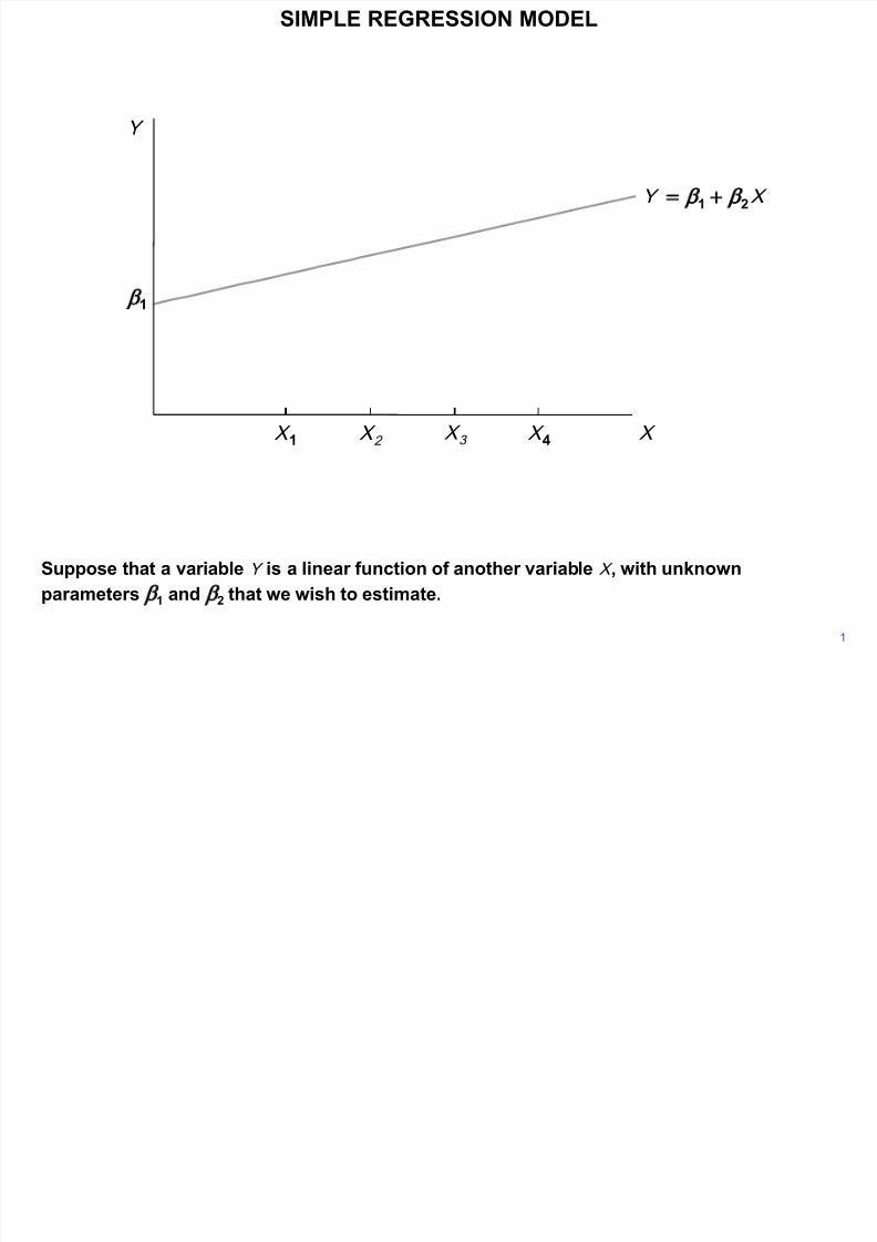
Suppose that we have a sample of 4 observations with X values as shown.
SIMPLE REGRESSION MODEL
2
X Y 21
1
Y
X X 1 X 2 X
3 X 4
8/12/2019 Dougherty (LSE, 2011) - Ref C1E1
http://slidepdf.com/reader/full/dougherty-lse-2011-ref-c1e1 3/25
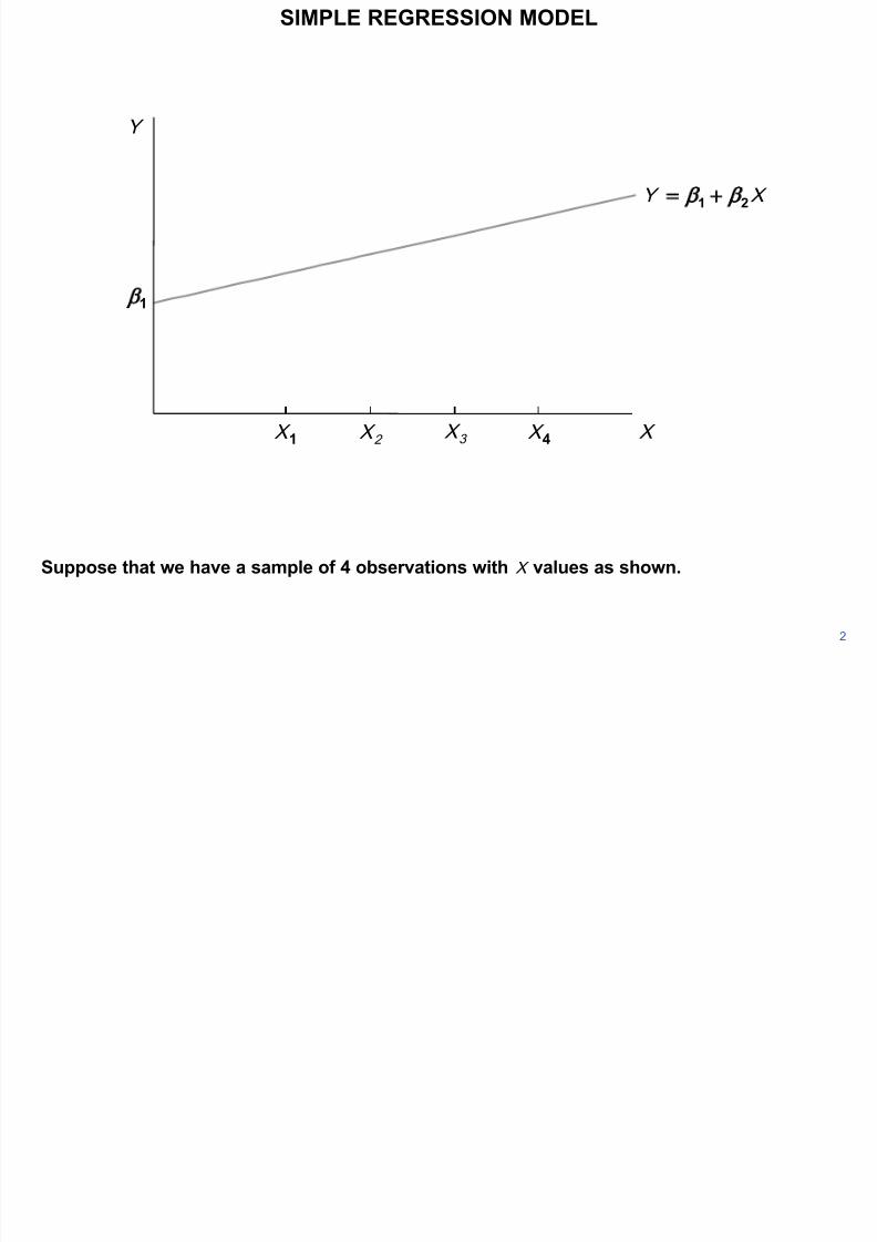
If the relationship were an exact one, the observations would lie on a straight line and we
would have no trouble obtaining accurate estimates of 1 and 2.
Q 1 Q 2 Q 3 Q 4
SIMPLE REGRESSION MODEL
3
X Y 21
1
Y
X X 1 X 2 X
3 X 4
8/12/2019 Dougherty (LSE, 2011) - Ref C1E1
http://slidepdf.com/reader/full/dougherty-lse-2011-ref-c1e1 4/25
P 4
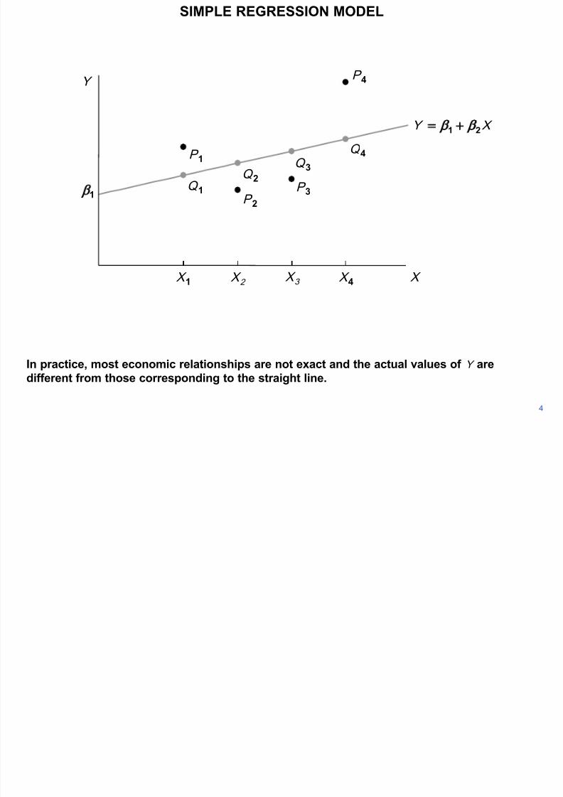
In practice, most economic relationships are not exact and the actual values of Y are
different from those corresponding to the straight line.
P 3
P 2
P 1 Q 1 Q 2 Q 3 Q 4
SIMPLE REGRESSION MODEL
4
X Y 21
1
Y
X X 1 X 2 X
3 X 4
8/12/2019 Dougherty (LSE, 2011) - Ref C1E1
http://slidepdf.com/reader/full/dougherty-lse-2011-ref-c1e1 5/25
P 4
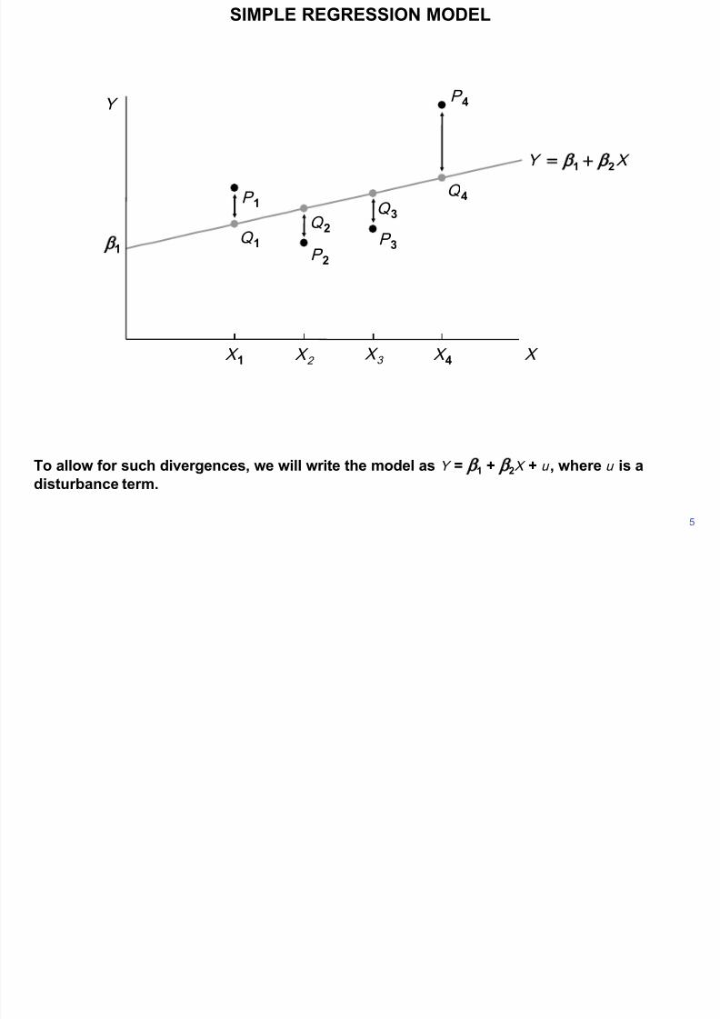
To allow for such divergences, we will write the model as Y = 1 + 2X + u , where u is a
disturbance term.
P 3
P 2
P 1 Q 1 Q 2 Q 3 Q 4
SIMPLE REGRESSION MODEL
5
X Y 21
1
Y
X X 1 X 2 X
3 X 4
8/12/2019 Dougherty (LSE, 2011) - Ref C1E1
http://slidepdf.com/reader/full/dougherty-lse-2011-ref-c1e1 6/25
P 4
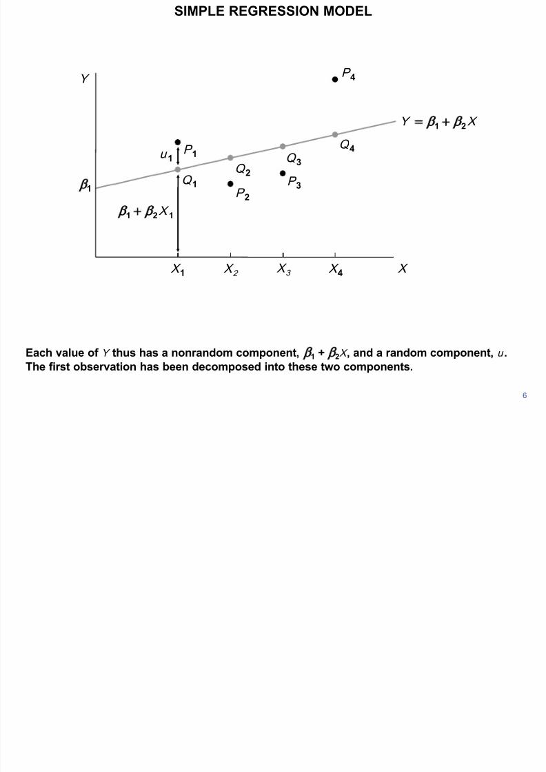
Each value of Y thus has a nonrandom component, 1 + 2X , and a random component, u .
The first observation has been decomposed into these two components.
P 3 P 2
P 1 Q 1 Q 2 Q 3 Q 4
u 1
SIMPLE REGRESSION MODEL
6
X Y 21
1
Y
121 X
X X 1 X 2 X
3 X 4
8/12/2019 Dougherty (LSE, 2011) - Ref C1E1
http://slidepdf.com/reader/full/dougherty-lse-2011-ref-c1e1 7/25
P 4
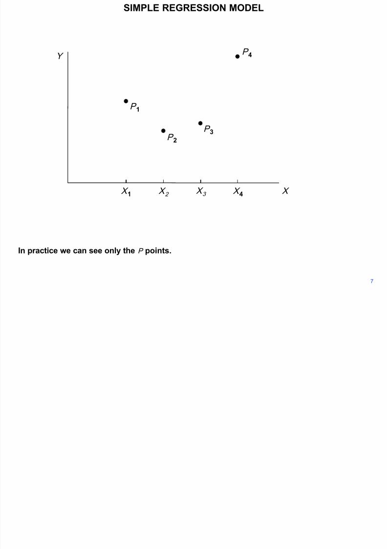
In practice we can see only the P points.
P 3 P 2
P 1
SIMPLE REGRESSION MODEL
7
Y
X X 1 X 2 X
3 X 4
8/12/2019 Dougherty (LSE, 2011) - Ref C1E1
http://slidepdf.com/reader/full/dougherty-lse-2011-ref-c1e1 8/25
P 4
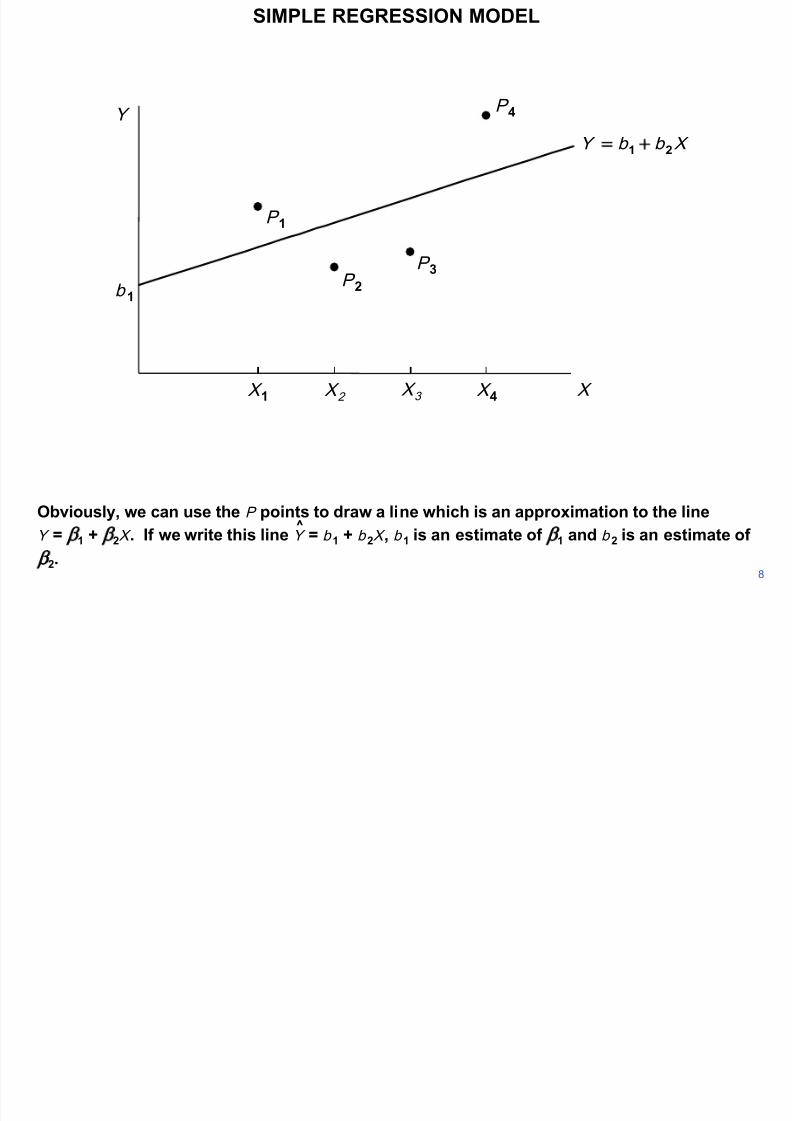
Obviously, we can use the P points to draw a line which is an approximation to the line
Y = 1 + 2X . If we write this line Y = b 1 + b 2X , b 1 is an estimate of 1 and b 2 is an estimate of
2.
P 3 P 2
P 1
^
SIMPLE REGRESSION MODEL
8
X b b Y 21ˆ
b 1
Y
X X 1 X 2 X
3 X 4
8/12/2019 Dougherty (LSE, 2011) - Ref C1E1
http://slidepdf.com/reader/full/dougherty-lse-2011-ref-c1e1 9/25
P 4
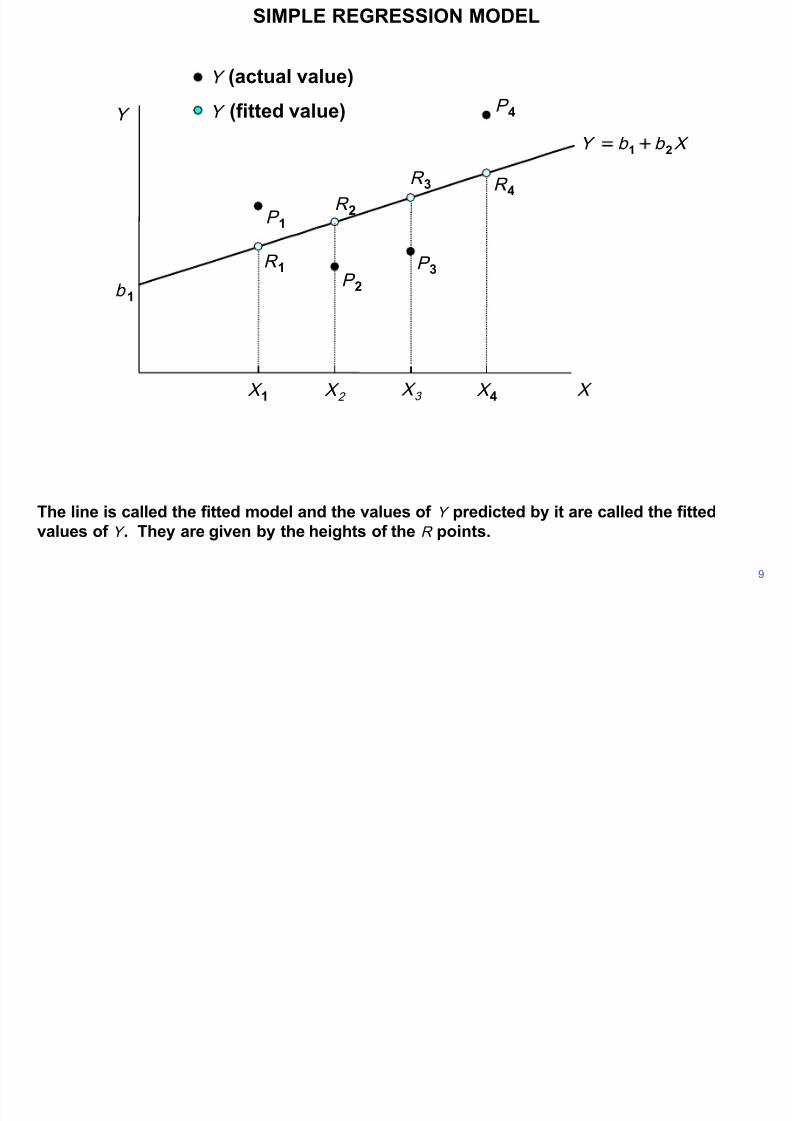
The line is called the fitted model and the values of Y predicted by it are called the fitted
values of Y . They are given by the heights of the R points.
P 3 P 2
P 1 R 1
R 2 R 3 R 4
SIMPLE REGRESSION MODEL
9
X b b Y 21ˆ
b 1
Y ̂(fitted value) Y (actual value)
Y
X X 1 X 2 X
3 X 4
8/12/2019 Dougherty (LSE, 2011) - Ref C1E1
http://slidepdf.com/reader/full/dougherty-lse-2011-ref-c1e1 10/25
P 4
X X 1 X 2 X
3 X 4
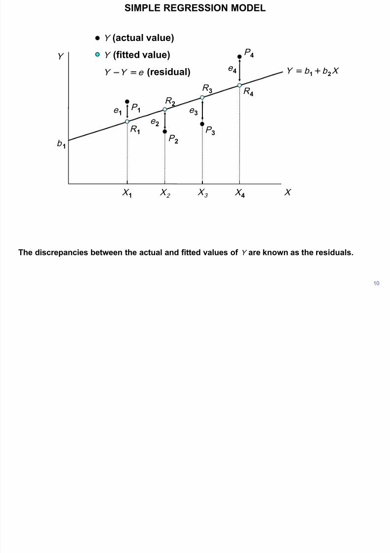
The discrepancies between the actual and fitted values of Y are known as the residuals.
P 3 P 2
P 1 R 1
R 2 R 3 R 4 (residual)
e 1 e 2
e 3
e 4
SIMPLE REGRESSION MODEL
10
X b b Y 21ˆ
b 1
Y ̂(fitted value) Y (actual value)
e Y Y ˆ
Y
8/12/2019 Dougherty (LSE, 2011) - Ref C1E1
http://slidepdf.com/reader/full/dougherty-lse-2011-ref-c1e1 11/25
P 4
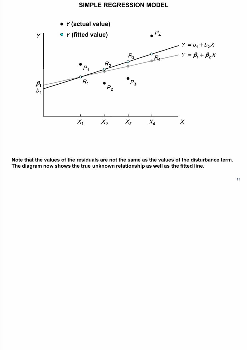
Note that the values of the residuals are not the same as the values of the disturbance term.
The diagram now shows the true unknown relationship as well as the fitted line.
P 3 P 2
P 1 R 1
R 2 R 3 R 4
b 1
SIMPLE REGRESSION MODEL
11
X b b Y 21ˆ
X Y 21
1
Y ̂(fitted value) Y (actual value)
Y
X X 1 X 2 X
3 X 4
8/12/2019 Dougherty (LSE, 2011) - Ref C1E1
http://slidepdf.com/reader/full/dougherty-lse-2011-ref-c1e1 12/25
P 4
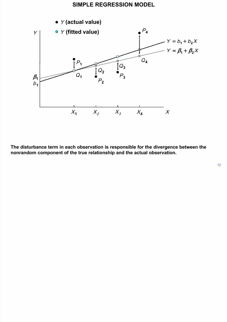
The disturbance term in each observation is responsible for the divergence between the
nonrandom component of the true relationship and the actual observation.
P 3 P 2
P 1
SIMPLE REGRESSION MODEL
12
Q 2 Q 1
Q 3 Q 4 X b b Y 21
ˆ
X Y 21
1
b 1
Y ̂(fitted value) Y (actual value)
Y
X X 1 X 2 X
3 X 4

8/12/2019 Dougherty (LSE, 2011) - Ref C1E1
http://slidepdf.com/reader/full/dougherty-lse-2011-ref-c1e1 13/25
P 4
The residuals are the discrepancies between the actual and the fitted values.
P 3 P 2
P 1 R 1
R 2 R 3 R 4
SIMPLE REGRESSION MODEL
13
X b b Y 21ˆ
X Y 21
1
b 1
Y ̂(fitted value) Y (actual value)
Y
X X 1 X 2 X
3 X 4
8/12/2019 Dougherty (LSE, 2011) - Ref C1E1
http://slidepdf.com/reader/full/dougherty-lse-2011-ref-c1e1 14/25
P 4
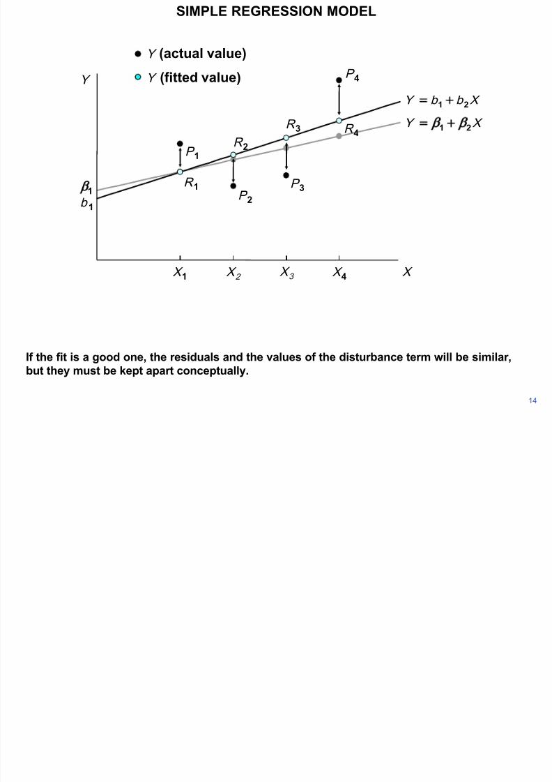
If the fit is a good one, the residuals and the values of the disturbance term will be similar,
but they must be kept apart conceptually.
P 3 P 2
P 1 R 1
R 2 R 3 R 4
SIMPLE REGRESSION MODEL
14
X b b Y 21ˆ
X Y 21
1
b 1
Y ̂(fitted value) Y (actual value)
Y
X X 1 X 2 X
3 X 4
8/12/2019 Dougherty (LSE, 2011) - Ref C1E1
http://slidepdf.com/reader/full/dougherty-lse-2011-ref-c1e1 15/25
SIMPLE REGRESSION MODEL
8/12/2019 Dougherty (LSE, 2011) - Ref C1E1
http://slidepdf.com/reader/full/dougherty-lse-2011-ref-c1e1 16/25
P 4
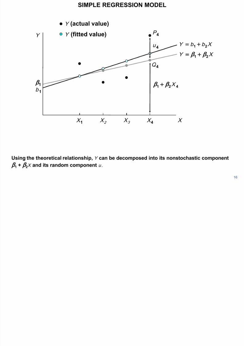
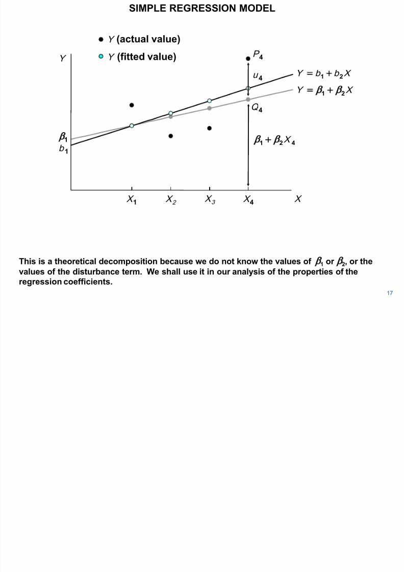
Using the theoretical relationship, Y can be decomposed into its nonstochastic component
1 + 2X and its random component u.
SIMPLE REGRESSION MODEL
16
Q 4 u 4 X b b Y 21
ˆ
X Y 21
1
b 1
Y ̂(fitted value) Y (actual value)
Y
421 X
X X 1 X 2 X
3 X 4
SIMPLE REGRESSION MODEL
8/12/2019 Dougherty (LSE, 2011) - Ref C1E1
http://slidepdf.com/reader/full/dougherty-lse-2011-ref-c1e1 17/25
P 4
This is a theoretical decomposition because we do not know the values of 1 or 2, or the
values of the disturbance term. We shall use it in our analysis of the properties of the
regression coefficients.
SIMPLE REGRESSION MODEL
17
Q 4 u 4 X b b Y 21
ˆ
X Y 21
1
b 1
Y ̂(fitted value) Y (actual value)
Y
421 X
X X 1 X 2 X
3 X 4
SIMPLE REGRESSION MODEL
8/12/2019 Dougherty (LSE, 2011) - Ref C1E1
http://slidepdf.com/reader/full/dougherty-lse-2011-ref-c1e1 18/25
P 4
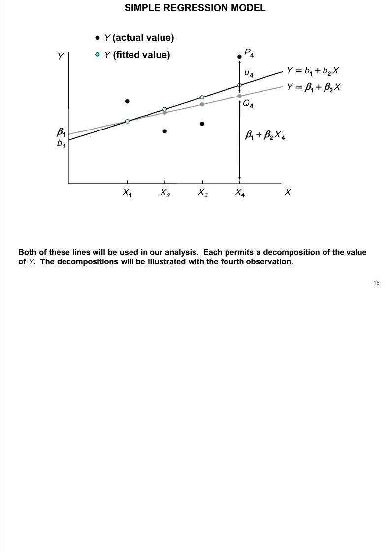
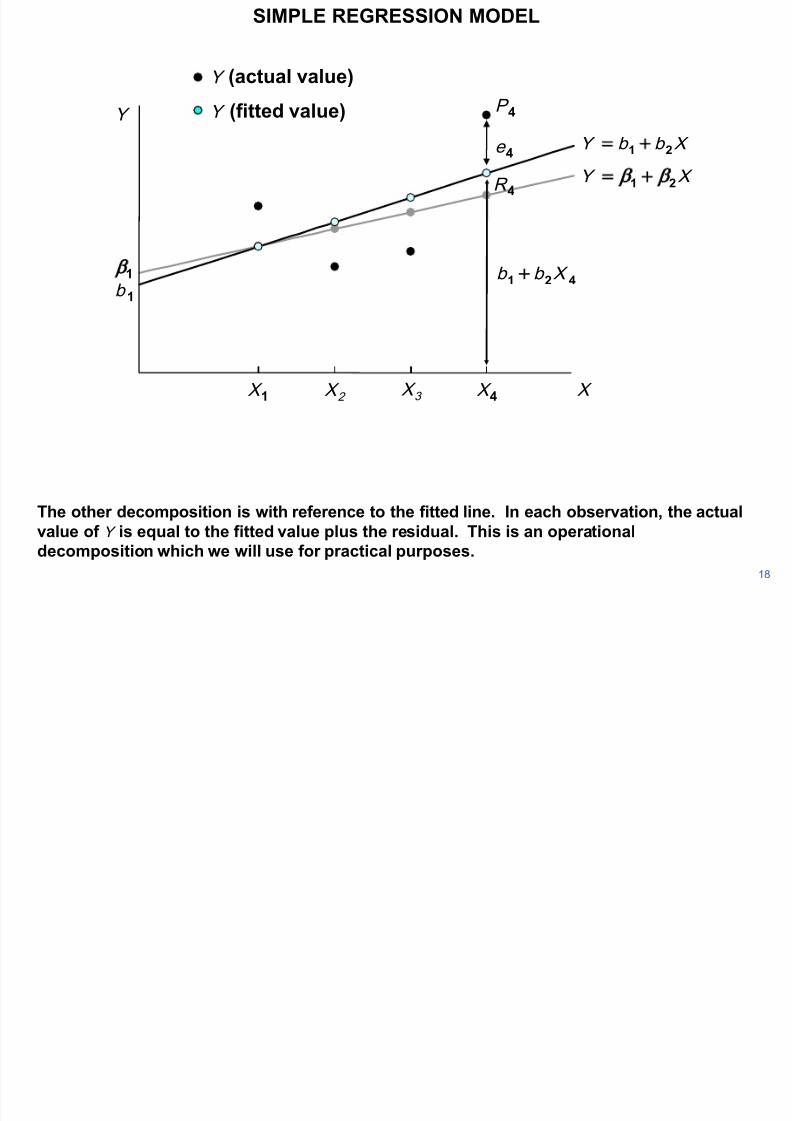
The other decomposition is with reference to the fitted line. In each observation, the actual
value of Y is equal to the fitted value plus the residual. This is an operational
decomposition which we will use for practical purposes.
SIMPLE REGRESSION MODEL
18
e 4 R 4
X b b Y 21ˆ
X Y 21
1
b 1
Y ˆ
Y (actual value) (fitted value) Y
421 X b b
X X 1 X 2 X
3 X 4
SIMPLE REGRESSION MODEL
8/12/2019 Dougherty (LSE, 2011) - Ref C1E1
http://slidepdf.com/reader/full/dougherty-lse-2011-ref-c1e1 19/25
SIMPLE REGRESSION MODEL
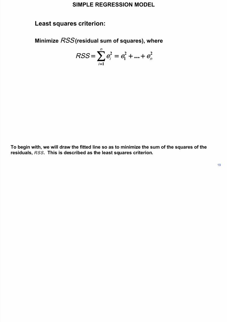
To begin with, we will draw the fitted line so as to minimize the sum of the squares of the
residuals, RSS . This is described as the least squares criterion. 19
Least squares criterion:
22
1
1
2...
n
n
i
i e e e RSS
Minimize RSS (residual sum of squares), where
SIMPLE REGRESSION MODEL
8/12/2019 Dougherty (LSE, 2011) - Ref C1E1
http://slidepdf.com/reader/full/dougherty-lse-2011-ref-c1e1 20/25
SIMPLE REGRESSION MODEL
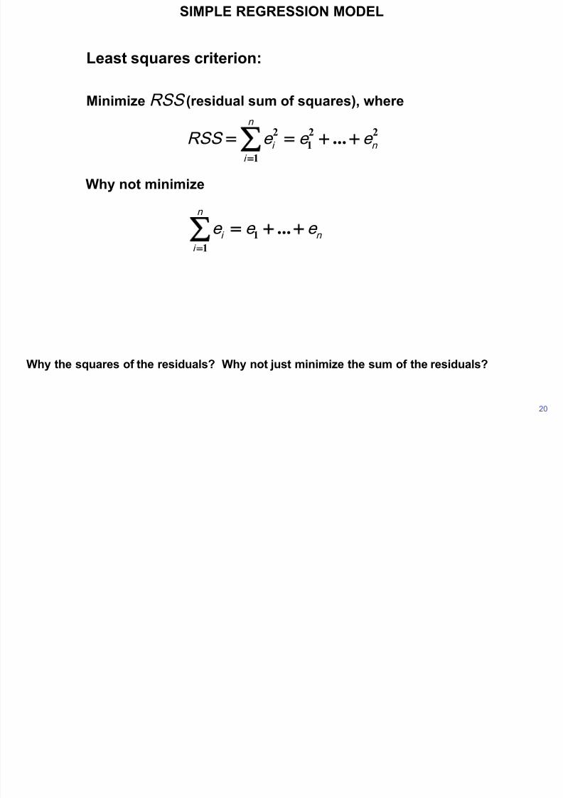
Why the squares of the residuals? Why not just minimize the sum of the residuals?
Least squares criterion:
Why not minimize
22
1
1
2...
n
n
i
i e e e RSS
n
n
i
i e e e
...1
1
20
Minimize RSS (residual sum of squares), where
SIMPLE REGRESSION MODEL
8/12/2019 Dougherty (LSE, 2011) - Ref C1E1
http://slidepdf.com/reader/full/dougherty-lse-2011-ref-c1e1 21/25
P 4
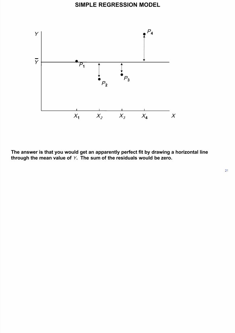
The answer is that you would get an apparently perfect fit by drawing a horizontal line
through the mean value of Y . The sum of the residuals would be zero.
P 3 P 2
P 1
SIMPLE REGRESSION MODEL
Y
21
X X 1 X 2 X
3 X 4
Y
SIMPLE REGRESSION MODEL
8/12/2019 Dougherty (LSE, 2011) - Ref C1E1
http://slidepdf.com/reader/full/dougherty-lse-2011-ref-c1e1 22/25
P 4
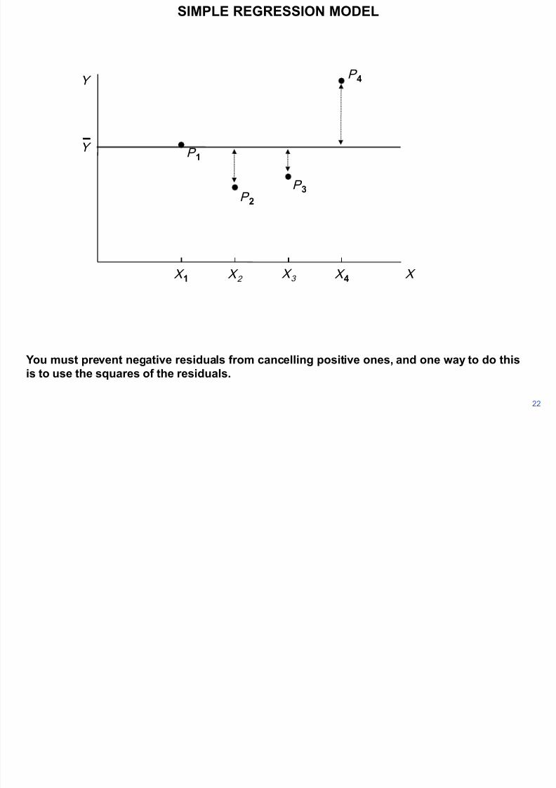
You must prevent negative residuals from cancelling positive ones, and one way to do this
is to use the squares of the residuals.
P 3 P 2
P 1
SIMPLE REGRESSION MODEL
22
X X 1 X 2 X
3 X 4
Y
Y
SIMPLE REGRESSION MODEL
8/12/2019 Dougherty (LSE, 2011) - Ref C1E1
http://slidepdf.com/reader/full/dougherty-lse-2011-ref-c1e1 23/25
P 4
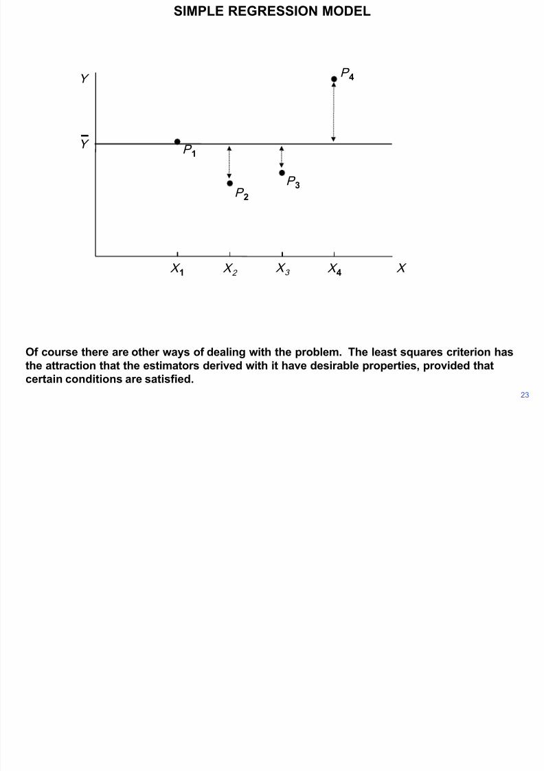
Of course there are other ways of dealing with the problem. The least squares criterion has
the attraction that the estimators derived with it have desirable properties, provided that
certain conditions are satisfied.
P 3 P 2
P 1
SIMPLE REGRESSION MODEL
23
X X 1 X 2 X
3 X 4
Y
Y
SIMPLE REGRESSION MODEL
8/12/2019 Dougherty (LSE, 2011) - Ref C1E1
http://slidepdf.com/reader/full/dougherty-lse-2011-ref-c1e1 24/25
P 4
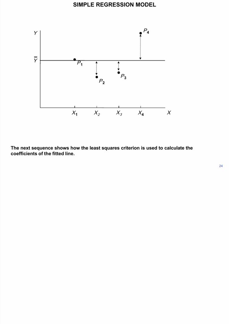
The next sequence shows how the least squares criterion is used to calculate the
coefficients of the fitted line.
P 3 P 2
P 1
SIMPLE REGRESSION MODEL
24
X X 1 X 2 X
3 X 4
Y
Y

8/12/2019 Dougherty (LSE, 2011) - Ref C1E1
http://slidepdf.com/reader/full/dougherty-lse-2011-ref-c1e1 25/25
Copyright Christopher Dougherty 2011.
These slideshows may be downloaded by anyone, anywhere for personal use.
Subject to respect for copyright and, where appropriate, attribution, they may be
used as a resource for teaching an econometrics course. There is no need to
refer to the author.
The content of this slideshow comes from Section 1.2 of C. Dougherty,
In troduct ion to Econ ometr ics , fourth edition 2011, Oxford University Press.
Additional (free) resources for both students and instructors may be
downloaded from the OUP Online Resource Centre
http://www.oup.com/uk/orc/bin/9780199567089/.
Individuals studying econometrics on their own and who feel that they might
benefit from participation in a formal course should consider the London School
of Economics summer school course
EC212 Introduction to Econometrics
http://www2.lse.ac.uk/study/summerSchools/summerSchool/Home.aspx or the University of London International Programmes distance learning course
20 Elements of Econometrics
www.londoninternational.ac.uk/lse.
11 07 25
Recommended