Journal of Science and Technology of the Arts, Volume 10, No. 1 – 2018
CITARJ 15
Drawing Equirectangular VR Panoramas with Ruler, Compass, and Protractor
António Bandeira Araújo Department of Science and Technology, Universidade Aberta, Portugal ----- [email protected] -----
ABSTRACT
This work presents a method for drawing Virtual
Reality panoramas by ruler and compass
operations. VR panoramas are immersive
anamorphoses rendered from equirectangular
spherical perspective data. This data is usually
photographic, but some artists are creating hand-
drawn equirectangular perspectives to be visualized
in VR. This practice, that lies interestingly at the
interface between analog and digital drawing, is
hindered by a lack of method, as these drawings are
usually done by trial-and-error, with ad-hoc
measurements and interpolation of pre-computed
grids, a process with considerable artistic limitations.
I develop here the analytic tools for plotting all great
circles, line images and their vanishing points, and
then show how to achieve these constructions
through descriptive geometry diagrams that can be
executed using only ruler, compass, and protractor.
Approximations of line images by circular arcs and
sinusoids are shown to have acceptable errors for
low values of angular elevation. The symmetries of
the perspective are studied and their uses for
improving gridding methods are discussed.
KEYWORDS
Visual arts; immersive art; immersive panoramas;
VR panoramas; equirectangular perspective;
spherical perspective; perspective; drawing;
descriptive geometry; digital art; ruler and compass;
social networks.
ARTICLE INFO
Received: 02 January 2018
Accepted: 21 February 2018
Published: 03 April 2018
https://dx.doi.org/10.7559/citarj.v10i1.471
1 | INTRODUCTION
1.1 PREVIOUS WORK
This work intends to settle equirectangular spherical
perspective as a proper perspective, by providing
clear and complete rules to solve all lines and
vanishing points, and a method for drawing them
with simple tools. It aims to bridge the gap between
traditional and digital drawing, in the creation of
immersive VR panoramas. This is a revision and
expansion of previous results I presented in a recent
conference paper (Araújo, 2017).
1.2 MOTIVATION
Artists are subverting Virtual Reality panoramas. VR
panoramas have been integrated into social
networking platforms mostly to accommodate
photographic pieces generated by 360-degree
cameras. Such cameras create equirectangular
spherical perspective pictures and the VR software
provides an immersive experience, by monitoring
the viewpoint of the user’s mobile phone or headset
and rendering at each instant a plane perspective of
a certain field of view from within the total picture.
Facebook, Google, and Flickr all provide simple
ways for the user to upload these pictures and share
them as VR, and specialized services keep popping
up, such as Kuula, offering new variations and
features for their display. But as this integration
grew, some artists started tentatively hand drawing –
rather than shooting - they own panoramas. Once
uploaded, these drawings will “look right” as VR
panoramas if they follow the rules of equirectangular
perspective. There’s an interesting collection of such
drawings appearing at Flickr’s artistic panorama
group (Art Panorama Group, 2017). See also the
whimsical examples by David Anderson (Anderson,
CITARJ 16
n.d.) and the virtuoso on-location drawing by Gérard
Michel (Michel, 2007; 2017).
This interest in drawing VR panoramas is part of a
trend. Illustrators and urban sketchers (the present
author hails from both tribes) seem of late rather
keen on curvilinear perspectives and
anamorphoses. Such waves of enthusiasm arise
whenever anamorphosis finds a new technological
expression. The current VR experience rehashes
that of once popular 19th century panoramas, for the
display of which large rotundas were built (Huhtamo,
2013), or the immersive spectacle of illusionary
church ceilings. These large scale immersive
anamorphoses were drawn out in plan and elevation
as if to build real architecture (and sometimes in
replacement of such, as in the case of Andrea
Pozzo’s famous dome at Sant’Ignazzio’s (Kemp,
1990), and then painted as a 2D simulacrum of the
imagined object. VR panorama drawings work much
the same way. Here too the artist starts with a flat
perspective drawing and aims at an immersive
experience. The obvious difference is in the
technology. A further, crucial difference, concerns us
here: When Andrea Pozzo did his illusionary work in
the late 1600s, he was firmly grounded in the
knowledge of linear perspective, as his treatise
attests (Pozzo, 1700); crudely put, he knew what he
was doing. By contrast, our VR panorama makers
have no handy equirectangular perspective manual
they can rely upon. What is available addresses
computer rendering, not human drawing. Artists do
without it in their usual fashion, being notorious
hackers of ad-hoc perspective, classical or
otherwise, who will - quite rightly! - cheat and fake it
if they must, by sheer trial-and-error, by drawing
over pre-computed grids or on top of photographs.
But it is lamentable to have to settle for such crude
methods. It can be argued that technology tends to
generate ignorance of the very processes it
streamlines (Stiegler, 2010), and this is true in
particular of the naive use of digital tools in art
(Rodriguez, 2016). That you can click a menu and
get a perspective grid does not enhance your
knowledge of perspective. It hinders it, by making it
unnecessary. That knowledge gets expressed in the
machine’s primitive operations rather than the
human’s (brute force plots rather than judicious ruler
and compass operations) and then black-boxed out
of view through abstraction and encapsulation,
which itself limits one’s modes of thought and
expression (Papert & Turkle, 1991); instead of
learning perspective you learn to turn knobs on a
black box whose interface delimits the scope of your
imagination. There is a knowledge of space and
form that you only get from drawing with your hands
and computing with your brain. That you can get a
perspective at the click of a button only makes it
more urgent that you know how to get one through
your mind and hands.
I argued, in a recent paper (Araújo, 2017b), for a
“deliberate rudimentarization” or “cardboarding” in
teaching the concepts behind digital tools - exposing
the conceptual gears of digital black boxes by
reducing them to their most basic physical
expression. The aim is to translate between the
human and the machine-executable, creating digital-
analog feedback loops that enhance the
understanding of both realms, and create spots for
artistic intervention upon the tools themselves. The
connection between anamorphoses, descriptive
geometry (DG) and Mixed Reality (MR) is one such
example of feedback loop. Through analog DG
techniques (Araújo, 2017a), the student can build
illusory objects that can be shared through digital
photography (the camera being the perfect cycloptic
eye of perspective), in a way that both motivates the
learning of DG techniques and illuminates the
operations behind MR tools. VR panoramas can
expand on this approach since they enable the
sharing in social networks not only of the static
photograph of the resulting anamorphosis, but the
actual immersive experience of the imagined
object’s visual presence. Note that curvilinear
perspectives are intimately related to
anamorphoses. A perspective can be seen as an
entailment of two maps - a conical anamorphosis
followed by a flattening (Araújo, 2015). Usually the
anamorphosis remains merely conceptual - although
some artists, notably Dick Termes (Termes, n.a.)
have explored it explicitly - as the artist works
directly on the perspective due to the convenience of
drawing on a plane. The VR display reverses the
entailment, allowing for an analog spherical
perspective, drawn by hand, to acquire its
anamorphic (mimetic) character. As a didactic tool
this allows the student to check the correctness of
his perspective construction in the most direct
manner. A curvilinear perspective drawing can be
hard to interpret, but an anamorphosis is judged by
eye: a line, planned out in spherical perspective,
either looks straight in VR or it doesn’t - allowing for
Journal of Science and Technology of the Arts, Volume 10, No. 1 – 2018
CITARJ 17
an experiential confirmation of the successful
perspective drawing. This specific type of
visualization will in turn feed back into the drawing
process, nor merely as a verification tool but as a
motivator of specific aesthetics (the VR display is a
reading mode and there is no such thing as a
passive reading mode) and therefore of the need to
solve geometric problems that derive from these
aesthetic goals.
But if the VR panorama is to have such didactic
applications, a clear method is required to plot the
perspectives by hand, not only within precomputed
grids (which are just another black box), but for all
general line projections. That is, one must solve the
perspective. This is what I propose here, in two
parts: First I develop the analytic and computational
tools for the systematic plotting of great circles,
straight line images and their vanishing points. Next,
I provide diagrammatic methods to achieve these
constructions without a computer, so as to draw
general equirectangular projections, from
observation or orthographic plans, using only ruler,
compass, and protractor.
2 | SOLVING EQUIRECTANGULAR
PERSPECTIVE
A spherical perspective can be defined as a conical
anamorphosis onto a sphere followed by a flattening
of the sphere onto a plane (Araújo, 2015). The
anamorphosis is just the central projection map 𝑃 ↦
𝑂𝑃⃗⃗⃗⃗ ⃗/|𝑂𝑃| where O is the center of the sphere,
representing the viewpoint. It is the same for any
spherical perspective, and turns spatial lines into
meridians with exactly two antipodal vanishing
points. Hence it is the choice of the flattening map
that distinguishes between spherical perspectives.
These flattenings are usually cartographic maps,
chosen for some useful property. For instance, the
most well-known example of a spherical perspective,
and the first to be solved by elementary means
(Barre & Flocon, 1964), was defined by choosing the
azimuthal equidistant map projection for its
flattening. In the anterior hemisphere, this flattening
shows low deformations and turns meridians into
(approximate) circular arcs (Barre, Flocon, &
Bouligand, 1964); in the posterior hemisphere, it
turns meridians into curves that are constructible
from circular arcs by simple ruler and compass
operations (Araújo, 2015). The simplicity of these
line projections makes it a strong choice for a hand-
drawn perspective. In contrast, equirectangular line
projections (meridians) are clearly not as simple as
arcs of circle, as can be seen in a comparison of the
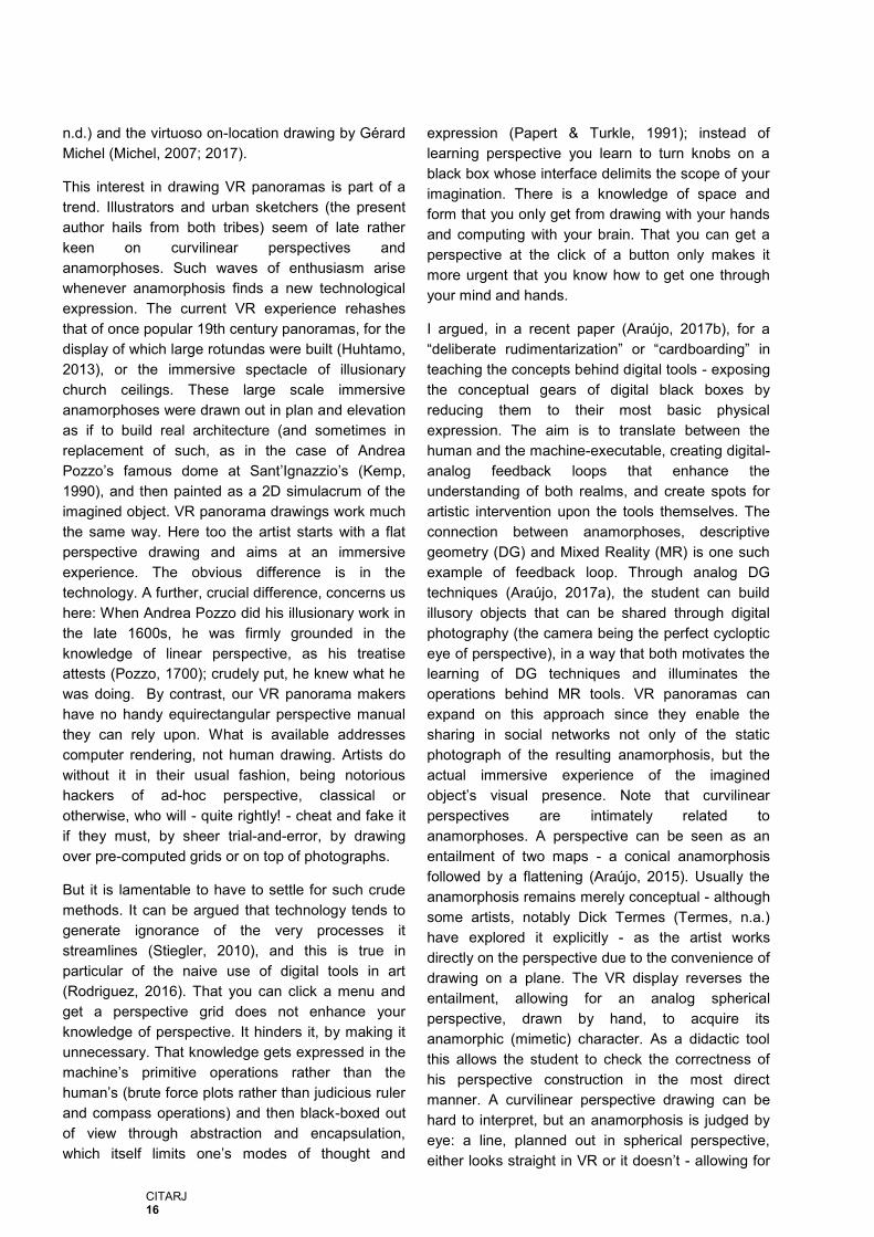
two projections in Figure 1. Equirectangular
perspective has, however, some important
advantages: it is the standard input for VR
panorama rendering engines, so it skips a
conversion step that tends to generate troublesome
artefacts; its coordinates correspond to the natural
angles that one measures in surveying; it renders
onto a rectangle rather than a disc, which accords
well both with image files and with the usual shape
of drawing pads, sketchbooks and picture frames;
and, as we shall see, it has many of the useful
features of cylindrical perspective with the
advantage of covering the whole field of view. For
all these reasons, it would be useful to solve this
perspective. To solve a perspective means to give a
classification of all lines and of their vanishing
points, and a method to plot them in practice. It also
implies a specification of means. Equirectangular
perspective is trivially plotted point-by-point by a
computer, but we want it to be solvable with simple
Figure 1 | Equirectangular panorama of a cubical room seen from its center (left), compared with azimuthal equidistant perspective of the same (right). Drawings by the author. The VR panorama rendering is available at the author’s website (Araújo, 2017c).
CITARJ 18
tools. The usual candidates are ruler and compass.
To tackle equirectangular perspective we need to
add to these a protractor.
2.1 THE EQUIRECTANGULAR MAP PROJECTION AND
ITS PERSPECTIVE
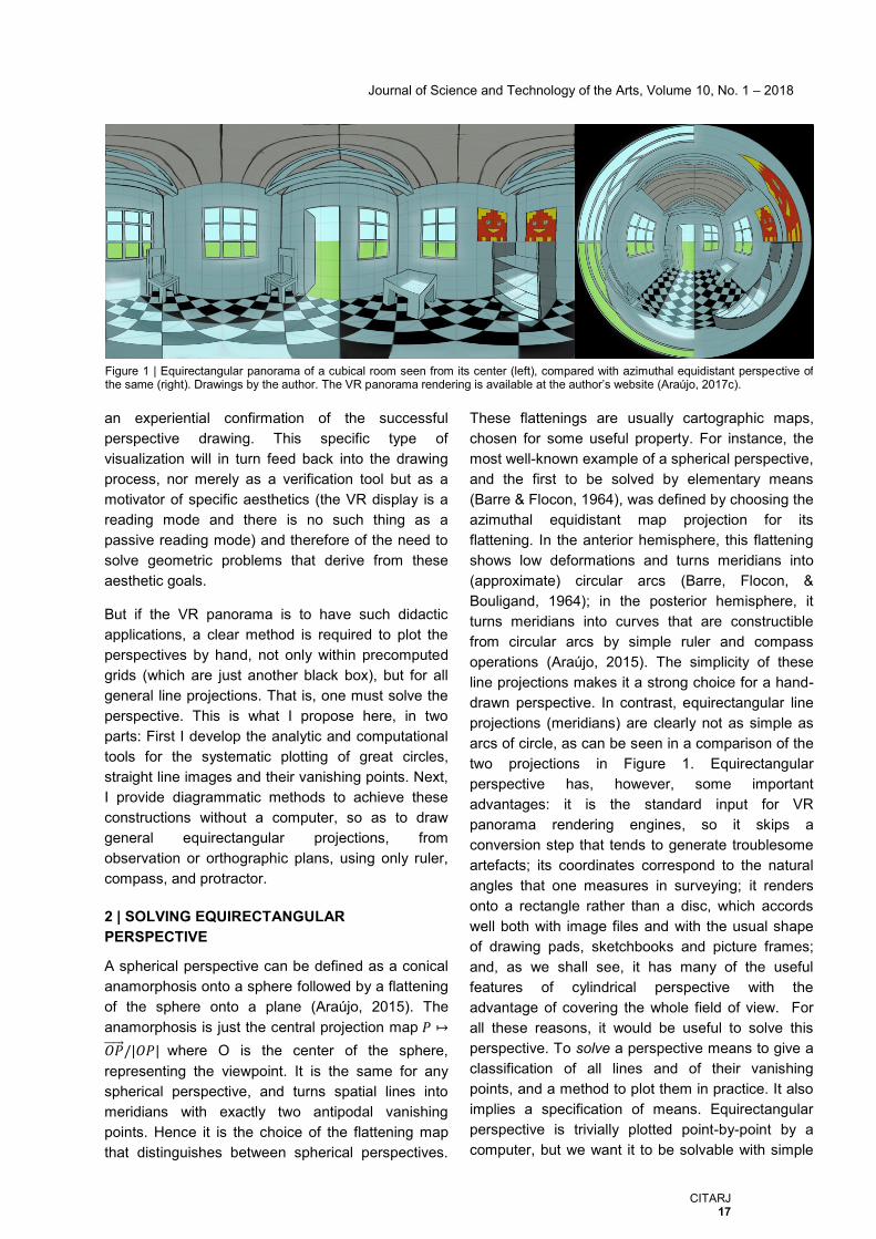
Let us define the equirectangular perspective image
of a point 𝑃. As discussed above, it is a two-step
process. 𝑃 is first projected radially onto the sphere
surface. Then that image point 𝑃’ is flattened onto
the plane by the equirectangular map projection.
This cartographic projection maps a point of the
sphere onto its longitude (λ) and latitude (φ)
coordinate pair, (λ, φ) (Snyder, 1987). It maps the
sphere onto the 2 × 1 rectangle ] − 180∘, 180∘[×] −
90∘, 90∘[ and turns parallels and (north-south)
meridians into horizontal and vertical straight lines,
respectively (Figure 2). Note that we will mostly
measure angles in degrees rather than radians
(asking the reader to mind the trigonometric
conversions assumed) since degrees are so
convenient for drawing (an A3 sheet will nicely fit a
360x180[mm] drawing rectangle, with longitudes in
the interval [-180mm,180mm] and latitudes in [-
90mm,90mm]. We choose a right-handed
orthonormal referential (𝑢𝑥⃗⃗⃗⃗ , 𝑢𝑦⃗⃗ ⃗⃗ , 𝑢𝑧⃗⃗⃗⃗ ) at the center of
the sphere O, such that (x, y) is the equatorial plane,
𝑢𝑧⃗⃗⃗⃗ points at the north pole, and 𝑂 + 𝑢𝑥⃗⃗⃗⃗ has zero
longitude. Then by simple trigonometry applied to
Figure 2, we see that φ = arcsin(𝑧/√𝑥2 + 𝑦2 + 𝑧2) .
As for 𝜆, it equals arctan(𝑦/𝑥) when 𝑥 > 0. For 𝑥 ≤
0 we must add or subtract 180º to this, for 𝑦 ≥ 0 or
𝑦 < 0 , respectively, and settle the 𝑥 = 0 case by
continuity. The case 𝑥 = 𝑦 = 0 is undefined. This is
neatly summed up by the function 𝑎𝑡𝑎𝑛2(𝑦, 𝑥) =
𝐴𝑟𝑔(𝑥 + 𝑖𝑦) , the so-called four-quadrant inverse
tangent, that verifies 𝑎𝑡𝑎𝑛2(cos(𝜃) , sin(𝜃)) = 𝜃 for
𝜃 ∈] − 180∘, 180∘] . Hence the equirectangular
perspective is given by the ℝ3 → ℝ2map
(𝜆, 𝜑) = (atan2(𝑦, 𝑥) , arcsin (𝑧
√𝑥2+𝑦2+𝑧2)).
This verifies the technical conditions for a curvilinear
perspective specified by (Araújo, 2015), namely: the
flattening is a homeomorphism in a dense open
subset of the sphere, and its inverse can be
extended to a continuous map between compact
sets. In fact, the flattening is one-to-one outside of
the north-south meridian 𝑚 that goes through
(−1,0,0) , and its inverse can be extended by
continuity to map the closed 2 × 1 rectangle to the
whole sphere, by the continuous map
(𝜆, 𝜑) ↦ (cos(𝜑) cos(𝜆) , cos(𝜑) sin(𝜆) , sin (𝜑))
that sends the top and bottom edges of the
rectangle to the north and south poles respectively,
and sends both vertical edges to the meridian 𝑚
(Figure 2).
2.2 ON LINES AND VANISHING POINTS
Solving a perspective requires a classification of
spatial lines and their vanishing points. How you
classify spatial lines depends on what you can
measure. An architect, drawing from plan and
elevation, can measure lengths. An astronomer
measures angles from a fixed point. The
draughtsman finds himself in the latter’s position
when drawing from life. I will now define what for
such a draughtsman may be a natural set of
variables to classify spatial lines.
Given a spatial line 𝑙, it is often possible to identify
the direction of the vertical plane H where it lies.
Suppose the viewer rotates (to a given longitude 𝜆0)
to face this plane. Then 𝑙 will extend 90 degrees to
his left and right, going to its vanishing points. The
Figure 2 | Equirectangular perspective and flattening. 𝑃 maps to 𝑃′ on the sphere by central projection and onto 𝑃′′ on the rectangle of the perspective drawing.
Journal of Science and Technology of the Arts, Volume 10, No. 1 – 2018
CITARJ 19
viewer can measure the incline of 𝑙 (the angle 𝜃 that
𝑙 makes with the horizontal through H) by tilting a
pencil on a plane parallel to H while visually
superimposing it on 𝑙 (the angle is preserved by
triangle similarity). Finally, he can measure the
angular elevation 𝜑0 at which 𝑙 passes in front of
him. We thus get coordinates (𝜆0, 𝜑0, 𝜃) that fully
specify line 𝑙.
Now we’d like to know how to plot such a line. If 𝑙 is
contained on a vertical plane through 𝑂(𝑂 ∉ 𝑙), then
it’s trivial: 𝑙 projects onto a vertical line (if 𝑙 is
vertical) or onto two antipodal vertical line segments
differing by 180º in longitude.
Let us consider then the non-trivial case: Let 𝑙 be a
spatial line such that 𝑂 ∉ 𝑙 and 𝑙 is not on a vertical
plane through 𝑂. We start by defining our three line
parameters more carefully: Let 𝑙′ be the orthogonal
projection of 𝑙 onto the equatorial plane. There is a
point 𝑄0 such that 𝑂𝑄0 and 𝑙′ define a right angle
(Figure 3). Let 𝜆0 be the longitude of 𝑄0 . Let 𝑃0 be
the point of 𝑙 lying on the vertical plane through 𝑂𝑄0.
Let 𝜑0 be the latitude of 𝑃0. Let 𝜃 to be the incline of
𝑙 , i.e., the angle between 𝑙 and 𝑙′ on the vertical
plane through 𝑙. We wish to plot a generic point 𝑃 on
the line 𝑙 of coordinates (𝜆0, 𝜑0, 𝜃) . We will
determine an expression 𝜑(𝜆) = 𝑓(𝜆|𝜆0, 𝜑0, 𝜃) for
the latitude 𝜑 of 𝑃 in terms of its longitude 𝜆. Let 𝑄
be the orthogonal projection of 𝑃 onto the equatorial
plane. Let Δ𝑥 = |𝑄0𝑄|, 𝑑0 = |𝑂𝑄0|, ℎ0 = |𝑄0𝑃0|. Then
𝜑(𝑃) = arctan (|𝑃𝑄|
|𝑄𝑂|) = arctan (
ℎ0 + tan(𝜃)Δ𝑥
√𝑑02 + Δ𝑥2
)
= arctan (ℎ0/𝑑0 + tan(𝜃)Δ𝑥/𝑑0
√1 + (Δ𝑥/𝑑0)2
)
= arctan (tan(𝜑0) + tan(𝜃)tan (𝜆 − 𝜆0 )
√1 + tan2(𝜆 − 𝜆0) )
= arctan(cos (λ − λ0)(tan (𝜑0) + tan(𝜃) tan(𝜆 − 𝜆0 )))
= arctan (tan(𝜑0) cos(𝜆 − 𝜆0) + tan (𝜃)sin (𝜆 − 𝜆0))
Hence the line of coordinates (𝜆0, 𝜑0, 𝜃) has
parametrization 𝜆 ↦ 𝜑(𝜆) = 𝑓(𝜆|𝜆0, 𝜑0, 𝜃)
= arctan(tan(𝜑0) cos(𝜆 − 𝜆0) + tan(𝜃) sin(𝜆 − 𝜆0)) (1)
where 𝜆 ∈ [𝜆0 − 𝜋/2, 𝜆0 + 𝜋/2 ].
Let us use this to plot some lines and get a feel for
their appearance. First, we note that spatial
rotational symmetries around the z axis become
translational symmetries for 𝜆 . We see that
𝑓(𝜆|𝜆0, 𝜑0, 𝜃) = 𝑓(𝜆 − 𝜆′|𝜆0 − 𝜆′, 𝜑0, 𝜃) for any 𝜆′ ; in
particular, 𝑓(𝜆|𝜆0, 𝜑0, 𝜃) = 𝑓(𝜆 − 𝜆0|0, 𝜑0, 𝜃) , so we
can draw any line as if it lies on the 𝜆0 = 0 vertical
plane, and then shift it sideways to its correct
position on the perspective plane. This reduces the
drawing problem to the 𝜆0 = 0 case.
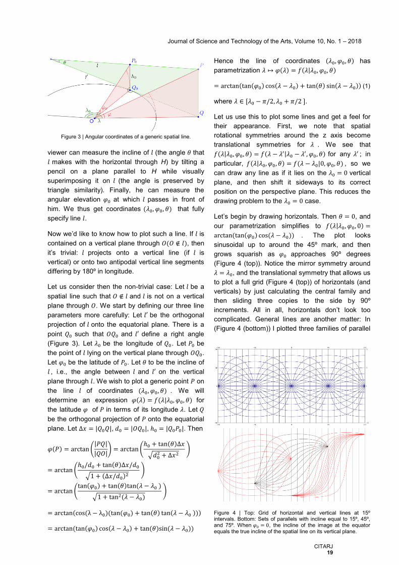
Let’s begin by drawing horizontals. Then 𝜃 = 0, and
our parametrization simplifies to 𝑓(𝜆|𝜆0, 𝜑0, 0) =
arctan(tan(𝜑0) cos(𝜆 − 𝜆0)) . The plot looks
sinusoidal up to around the 45º mark, and then
grows squarish as 𝜑0 approaches 90º degrees
(Figure 4 (top)). Notice the mirror symmetry around
𝜆 = 𝜆0, and the translational symmetry that allows us
to plot a full grid (Figure 4 (top)) of horizontals (and
verticals) by just calculating the central family and
then sliding three copies to the side by 90º
increments. All in all, horizontals don’t look too
complicated. General lines are another matter: In
(Figure 4 (bottom)) I plotted three families of parallel
Figure 3 | Angular coordinates of a generic spatial line.
Figure 4 | Top: Grid of horizontal and vertical lines at 15º intervals. Bottom: Sets of parallels with incline equal to 15º, 45º, and 75º. When 𝜑0 = 0, the incline of the image at the equator equals the true incline of the spatial line on its vertical plane.
CITARJ 20
lines. From left to right we have 𝜃 =15º, 45º and 75º,
with 𝜆0 = −90º, 0º, 90º respectively, and lines in
each family separated by intervals of 15 degrees of
latitude. We see that as 𝜃 grows the lines become
S-shaped, and then progressively sigmoidal, with
the maximum of the curve being reached closer and
closer to the vanishing point. Individual lines are no
longer mirror symmetric across the 𝜆 = 𝜆0 axis, only
the 𝜑0 = 0 line of each family retaining central
symmetry. These curves seem rather daunting to
the unaided analog artist!
Fortunately, there is a way to reduce all lines to the
𝜃 = 0 case. In any spherical perspective is it always
smart to draw a line by first drawing its great circle
and then finding the line inside it. A line projected on
a sphere is always a meridian (half of a great circle),
and a great circle projects either as a vertical or as a
union of two horizontals (Figure 5) oriented at some
angle 𝜆𝑀. We will find that angle, those horizontals,
and our line within them, as a subset delimited by its
two vanishing points. Start by recalling some
spherical geometry: The antipodal point of a point 𝑃
is the point 𝑃⋆ diametrically opposite to it on the
sphere. If 𝑃 = (𝜆, 𝜑) then 𝑃⋆ = (𝜆 − 𝑠𝑔𝑛(𝜆)𝜋, −𝜑)
where 𝑠𝑔𝑛(𝑥) = 𝑥/|𝑥| . A great circle is the
intersection of the sphere with a plane through its
center. A spatial line defines such a plane; Hence a
spatial line defines a single great circle and projects
as a meridian, the great circle being the union of two
meridians whose points are antipodal to each other.
The vanishing points of the line, that delimit it inside
its great circle, are obtained (in any central
perspective) by translating the line to 𝑂 and
intersecting with the sphere. Hence a line (𝜆0, 𝜑0, 𝜃)
has vanishing points at 𝑣1 = (𝜆0 − 𝑠𝑔𝑛(𝜆0)𝜋, 𝜃) and
at its antipode 𝑣1⋆ . We now note that our
parametrization of a line (hence, of a meridian) can
already be used to plot the whole great circle that
contains it, simply by extending its domain while
preserving its functional form. In fact, let 𝐶 be the
great circle of 𝑙. Then the perspective image of 𝐶 is
the union of the image of 𝑙 with the set of the images
of the antipodal points of 𝑙. But from eq. 1 we see
that 𝜑(𝜆 − 𝑠𝑔𝑛(𝜆)𝜋|𝜆0, 𝜑0, 𝜃) = −𝜑(𝜆|𝜆0, 𝜑0, 𝜃), since
the sin and cos reverse sign and arctan is odd, so
the function 𝜆 ↦ 𝑓(𝜆|𝜆0, 𝜑0, 𝜃) already parametrizes
the whole great circle of 𝑙 if we extend its domain to
[𝜆0 − 𝜋, 𝜆0 + 𝜋] . Further, we can rewrite the
parametrization to get a single cosine in the arctan
argument. Just set 𝐶 cos(𝜆 − 𝜆𝑀) = tan(𝜑0) cos(𝜆 −
𝜆0) + tan(𝜃) sin(𝜆 − 𝜆0) for unknown 𝜆𝑀 , 𝐶 . Setting
𝜆 = 𝜆0we get 𝐶 cos(𝜆0 − 𝜆𝑀) = tan(𝜑0) , and setting
𝜆 = 𝜆0 + 𝜋/2 we get 𝐶 sin(𝜆0 − 𝜆𝑀) = − tan(𝜃 ) ,
whence C2 = tan2(𝜑0) + tan2(𝜃) and 𝜆𝑀 = 𝜆0 +
arctan(tan(𝜃)/ tan(𝜑0)) . Then the parametrization
of the great circle containing line (𝜆0, 𝜑0, 𝜃) takes the
form
𝑔(𝜆|𝜆𝑀, 𝜑𝑀) = arctan(tan(𝜑𝑀) cos(𝜆 − 𝜆𝑀)) (2)
where 𝜆 ∈ [−𝜋, 𝜋], and
𝜆𝑀 = 𝜆0 + arctan(tan(𝜃)/ tan(𝜑0)),
𝜑𝑀 = arctan(√tan(𝜑0) + tan(𝜃) ).
We see that a great circle is therefore described by
the pair of parameters (𝜆𝑀, 𝜑𝑀) . We have
𝑓(𝜆|𝜆0, 𝜑0, 𝜃) = 𝑔(𝜆|𝜆𝑀, 𝜑𝑀) when 𝜆 ∈ [𝜆0 − 𝜋/2, 𝜆0 +
𝜋/2], so that both parametrize the same line in a
given window of width 𝜋. But notice that (2) has the
functional form the plot of a horizontal! It is the plot
of the horizontal (𝜆𝑀, 𝜑𝑀 , 0) when 𝜆 is in the interval
[𝜆𝑀 − 𝜋, 𝜆𝑀 + 𝜋] and of its antipode (𝜆𝑀 ± 𝜋,−𝜑𝑀 , 0)
outside of that interval. That means we can draw
any line by drawing horizontals and clipping them at
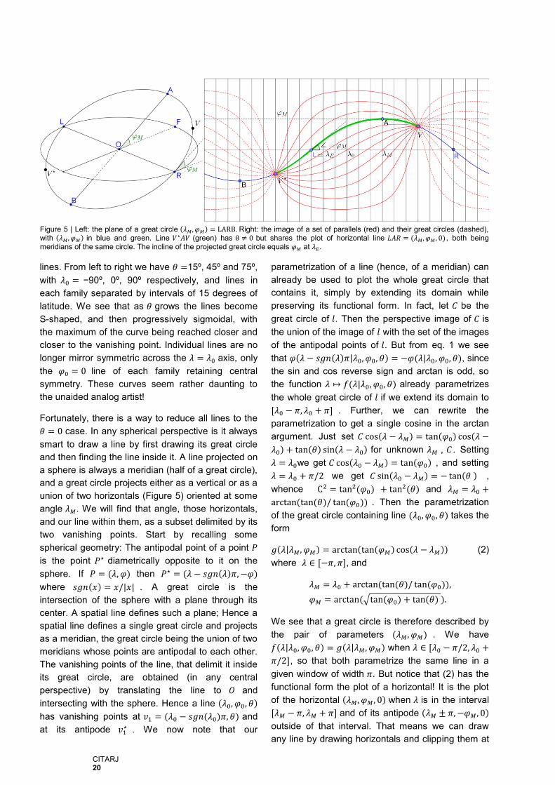
Figure 5 | Left: the plane of a great circle (𝜆𝑀, 𝜑𝑀) = LARB. Right: the image of a set of parallels (red) and their great circles (dashed), with (𝜆𝑀, 𝜑𝑀) in blue and green. Line 𝑉⋆𝐴𝑉 (green) has θ ≠ 0 but shares the plot of horizontal line 𝐿𝐴𝑅 = (𝜆𝑀, 𝜑𝑀 , 0), both being meridians of the same circle. The incline of the projected great circle equals 𝜑𝑀 at 𝜆𝐸.
Journal of Science and Technology of the Arts, Volume 10, No. 1 – 2018
CITARJ 21
the line’s vanishing points! Figure 5 clarifies the
geometric meaning of the pair 𝜆𝑀, 𝜑𝑀. On Figure 5
(left) we see a great circle 𝐶 = 𝐴𝑅𝐵𝐿 and on Figure
5 (right) its perspective image (blue and green line).
The plane of the great circle intersects the equatorial
plane at a line 𝐿𝑅 and makes an angle 𝜑𝑀 with it.
This angle equals the maximum latitude reached by
𝐶 , at point 𝐴 with longitude 𝜆𝑀 . Note that 𝜑𝑀 also
equals the incline of the tangent at the latitude 𝜆𝐸
where the circle crosses the equator. Since tangents
are preserved at the equator, the plot has incline
𝜑𝑀 at longitude 𝜆𝐸 . This and the zero incline at 𝜆𝑀
gives the draughtsman useful control points for the
tangents. Note that a line with 𝜆0 = 𝜆𝐸 has 𝜃 = 𝜑𝑀; a
line with 𝜃 = 0 has incline 𝜑0 = 𝜑𝑀 at its vanishing
points; and a line with 𝜑0 = 0 has latitude 𝜃 = 𝜑𝑀 at
its vanishing points. 𝜆𝑀 and 𝜑𝑀 define the circle
uniquely, but there are many meridians (lines) in it;
we write 𝑙 ≡ 𝑙′ when lines 𝑙, 𝑙′ share the same great
circle. To specify a line, we set either 𝜆0 or a
vanishing point 𝑉 . This defines a 180º clipping
window (the interval [𝜆0 − 𝜋, 𝜆0 + 𝜋] ) where line
𝑉⋆𝐴𝑉 (in green on Figure 5, right) lies on the plot of
the complete great circle (in blue). Note that on the
plot, latitude rises from 𝑉⋆ , goes to zero at 𝜆𝐸 ,
passes through 𝜑0 and reaches its maximum over
𝜆𝑀 , then declines towards 𝑉. It has incline 𝜑𝑀 at
longitude 𝜆𝐸 , as discussed. We see that the
asymmetrical plot of the line is just a section of the
more symmetrical plot of the great circle in blue, and
this is just the union of two mirrored horizontals. In
fact, (𝜆𝑀 − 𝜋/2,0, 𝜑𝑀) ≡ (𝜆𝑀, 𝜑𝑀 , 0) . We illustrate
this for a family of parallels. In Figure 5 (right) we
draw in filled red. They have vanishing points at
(±90∘, ±30∘) , so 𝜆0 = 0 , and their range is
[−90∘, 90∘]. They all have incline 𝜃 = 30∘ and differ
by 15º increments in 𝜆0. By plotting their full circles
(dashed red) we see how they are nothing more
than a plot of horizontals as in the grid of Figure 4
and the asymmetry is an artefact of their sampling
by the clipping window. All we need to draw are
horizontals (𝜃 = 0) lines and their lateral
translations. For instance, for our green line, which
is (0, 30∘, 30∘), we obtain from the definitions in eq. 2
that 𝜆𝑀 = 45∘ and 𝜑𝑀 = arctan(√(2/3)) ≈ 39∘, so we
plot the horizontals (45∘, 39∘, 0) and (135∘, −39∘, 0)
which together make up the circle (45∘, 39∘) , and
then clip it at 𝜆 = ±90∘. Of course we’d rather not
use the expressions of eq. 2 to obtain (𝜆𝑀, 𝜑𝑀). We
don’t wish to draw with calculator in hand. But we
can measure them directly from observation. On the
domain of a line you always have one of the
extremes and one points where it hits the equator. If
𝜆𝐸 is easier to spot, find it and you know 𝜆𝑀 is 90º
away; then measure the angular height at 𝜆𝑀 to get
𝜑𝑀. Or measure the incline at 𝜆𝐸, and recall it must
equal 𝜑𝑀. For instance, for our blue line, the incline
at 𝜆𝐸 = 45∘ is 𝜑𝑀 ≈ 39∘.
2.3 PLOTTING WITH RULER, COMPASS AND
PROTRACTOR
We have reduced all line plots to those of type
(0, 𝜑𝑀, 0) , modulo translation and choice of
vanishing points. It remains to show how to plot
these lines by elementary means, using ruler,
compass, and protractor, rather than computers or
calculators. We will do it with some simple
descriptive geometry diagrams.
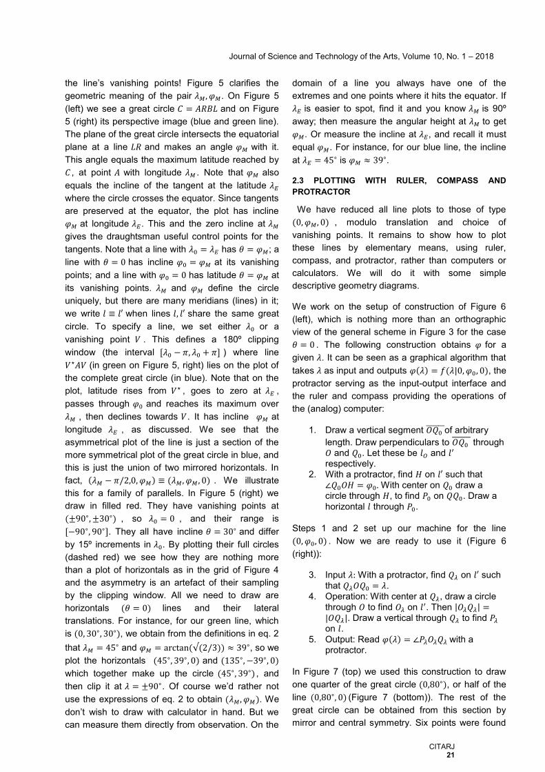
We work on the setup of construction of Figure 6
(left), which is nothing more than an orthographic
view of the general scheme in Figure 3 for the case
𝜃 = 0 . The following construction obtains 𝜑 for a
given 𝜆. It can be seen as a graphical algorithm that
takes 𝜆 as input and outputs 𝜑(𝜆) = 𝑓(𝜆|0, 𝜑0, 0), the
protractor serving as the input-output interface and
the ruler and compass providing the operations of
the (analog) computer:
1. Draw a vertical segment 𝑂𝑄0 ̅̅ ̅̅ ̅̅ of arbitrary
length. Draw perpendiculars to 𝑂𝑄0 through 𝑂 and 𝑄0. Let these be 𝑙𝑂 and 𝑙′ respectively.
2. With a protractor, find 𝐻 on 𝑙′ such that
∠𝑄0𝑂𝐻 = 𝜑0. With center on 𝑄0 draw a circle through 𝐻, to find 𝑃0 on 𝑄𝑄0. Draw a
horizontal 𝑙 through 𝑃0.
Steps 1 and 2 set up our machine for the line
(0, 𝜑0, 0) . Now we are ready to use it (Figure 6
(right)):
3. Input 𝜆: With a protractor, find 𝑄𝜆 on 𝑙′ such
that 𝑄𝜆𝑂𝑄0 = 𝜆. 4. Operation: With center at 𝑄𝜆, draw a circle
through 𝑂 to find 𝑂𝜆 on 𝑙′. Then |𝑂𝜆𝑄𝜆| =|𝑂𝑄𝜆|. Draw a vertical through 𝑄𝜆 to find 𝑃𝜆 on 𝑙.
5. Output: Read 𝜑(𝜆) = ∠𝑃𝜆𝑂𝜆𝑄𝜆 with a protractor.
In Figure 7 (top) we used this construction to draw
one quarter of the great circle (0,80∘), or half of the
line (0,80∘, 0) (Figure 7 (bottom)). The rest of the
great circle can be obtained from this section by
mirror and central symmetry. Six points were found
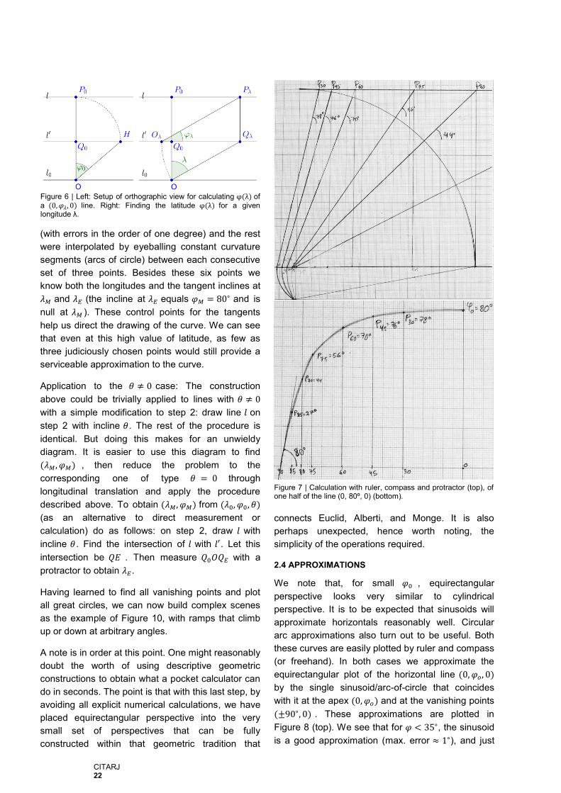
CITARJ 22
(with errors in the order of one degree) and the rest
were interpolated by eyeballing constant curvature
segments (arcs of circle) between each consecutive
set of three points. Besides these six points we
know both the longitudes and the tangent inclines at
𝜆𝑀 and 𝜆𝐸 (the incline at 𝜆𝐸 equals 𝜑𝑀 = 80∘ and is
null at 𝜆𝑀 ). These control points for the tangents
help us direct the drawing of the curve. We can see
that even at this high value of latitude, as few as
three judiciously chosen points would still provide a
serviceable approximation to the curve.
Application to the 𝜃 ≠ 0 case: The construction
above could be trivially applied to lines with 𝜃 ≠ 0
with a simple modification to step 2: draw line 𝑙 on
step 2 with incline 𝜃. The rest of the procedure is
identical. But doing this makes for an unwieldy
diagram. It is easier to use this diagram to find
(𝜆𝑀 , 𝜑𝑀) , then reduce the problem to the
corresponding one of type 𝜃 = 0 through
longitudinal translation and apply the procedure
described above. To obtain (𝜆𝑀, 𝜑𝑀) from (𝜆0, 𝜑0, 𝜃)
(as an alternative to direct measurement or
calculation) do as follows: on step 2, draw 𝑙 with
incline 𝜃. Find the intersection of 𝑙 with 𝑙′. Let this
intersection be 𝑄𝐸 . Then measure 𝑄0𝑂𝑄𝐸 with a
protractor to obtain 𝜆𝐸.
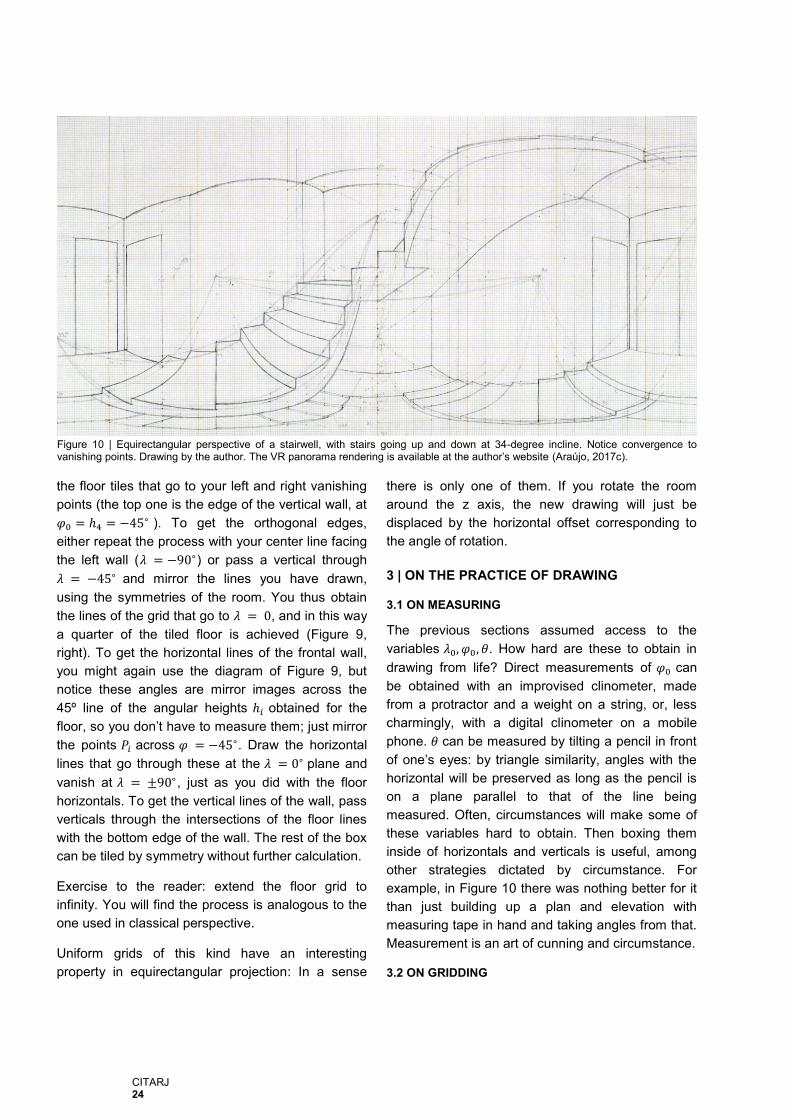
Having learned to find all vanishing points and plot
all great circles, we can now build complex scenes
as the example of Figure 10, with ramps that climb
up or down at arbitrary angles.
A note is in order at this point. One might reasonably
doubt the worth of using descriptive geometric
constructions to obtain what a pocket calculator can
do in seconds. The point is that with this last step, by
avoiding all explicit numerical calculations, we have
placed equirectangular perspective into the very
small set of perspectives that can be fully
constructed within that geometric tradition that
connects Euclid, Alberti, and Monge. It is also
perhaps unexpected, hence worth noting, the
simplicity of the operations required.
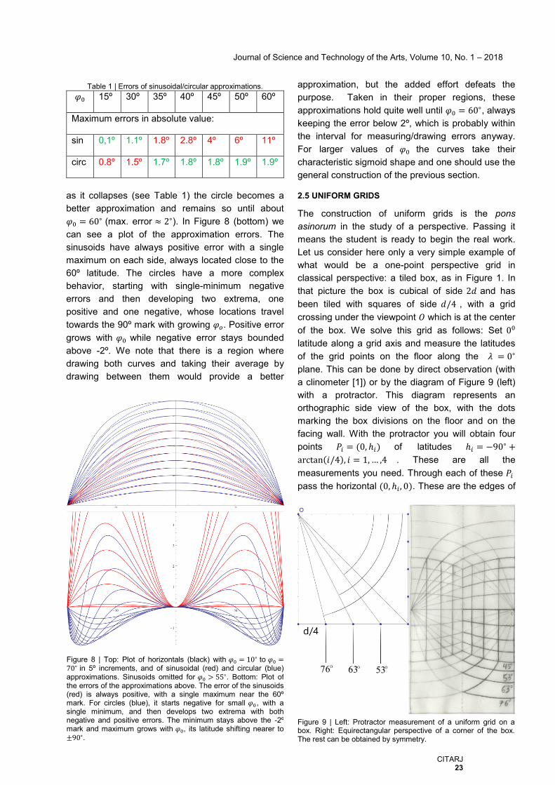
2.4 APPROXIMATIONS
We note that, for small 𝜑0 , equirectangular
perspective looks very similar to cylindrical
perspective. It is to be expected that sinusoids will
approximate horizontals reasonably well. Circular
arc approximations also turn out to be useful. Both
these curves are easily plotted by ruler and compass
(or freehand). In both cases we approximate the
equirectangular plot of the horizontal line (0, 𝜑𝑜, 0)
by the single sinusoid/arc-of-circle that coincides
with it at the apex (0, 𝜑𝑜) and at the vanishing points
(±90∘, 0) . These approximations are plotted in
Figure 8 (top). We see that for 𝜑 < 35∘, the sinusoid
is a good approximation (max. error ≈ 1∘), and just
Figure 6 | Left: Setup of orthographic view for calculating φ(λ) of
a (0,𝜑𝜆 , 0) line. Right: Finding the latitude φ(λ) for a given longitude λ.
Figure 7 | Calculation with ruler, compass and protractor (top), of one half of the line (0, 80º, 0) (bottom).
Journal of Science and Technology of the Arts, Volume 10, No. 1 – 2018
CITARJ 23
as it collapses (see Table 1) the circle becomes a
better approximation and remains so until about
𝜑0 = 60∘ (max. error ≈ 2∘). In Figure 8 (bottom) we
can see a plot of the approximation errors. The
sinusoids have always positive error with a single
maximum on each side, always located close to the
60º latitude. The circles have a more complex
behavior, starting with single-minimum negative
errors and then developing two extrema, one
positive and one negative, whose locations travel
towards the 90º mark with growing 𝜑𝑜. Positive error
grows with 𝜑0 while negative error stays bounded
above -2º. We note that there is a region where
drawing both curves and taking their average by
drawing between them would provide a better
approximation, but the added effort defeats the
purpose. Taken in their proper regions, these
approximations hold quite well until 𝜑0 = 60∘, always
keeping the error below 2º, which is probably within
the interval for measuring/drawing errors anyway.
For larger values of 𝜑0 the curves take their
characteristic sigmoid shape and one should use the
general construction of the previous section.
2.5 UNIFORM GRIDS
The construction of uniform grids is the pons
asinorum in the study of a perspective. Passing it
means the student is ready to begin the real work.
Let us consider here only a very simple example of
what would be a one-point perspective grid in
classical perspective: a tiled box, as in Figure 1. In
that picture the box is cubical of side 2𝑑 and has
been tiled with squares of side 𝑑/4 , with a grid
crossing under the viewpoint 𝑂 which is at the center
of the box. We solve this grid as follows: Set 00
latitude along a grid axis and measure the latitudes
of the grid points on the floor along the 𝜆 = 0∘
plane. This can be done by direct observation (with
a clinometer [1]) or by the diagram of Figure 9 (left)
with a protractor. This diagram represents an
orthographic side view of the box, with the dots
marking the box divisions on the floor and on the
facing wall. With the protractor you will obtain four
points 𝑃𝑖 = (0, ℎ𝑖) of latitudes ℎ𝑖 = −90∘ +
arctan(𝑖/4), 𝑖 = 1,… ,4 . These are all the
measurements you need. Through each of these 𝑃𝑖
pass the horizontal (0, ℎ𝑖 , 0). These are the edges of
Table 1 | Errors of sinusoidal/circular approximations.
𝜑0 15º 30º 35º 40º 45º 50º 60º
Maximum errors in absolute value:
sin 0,1º 1.1º 1.8º 2.8º 4º 6º 11º
circ 0.8º 1.5º 1.7º 1.8º 1.8º 1.9º 1.9º
Figure 8 | Top: Plot of horizontals (black) with 𝜑0 = 10∘ to 𝜑0 =70∘ in 5º increments, and of sinusoidal (red) and circular (blue) approximations. Sinusoids omitted for 𝜑0 > 55∘. Bottom: Plot of the errors of the approximations above. The error of the sinusoids (red) is always positive, with a single maximum near the 60º mark. For circles (blue), it starts negative for small 𝜑0 , with a single minimum, and then develops two extrema with both negative and positive errors. The minimum stays above the -2º mark and maximum grows with 𝜑0, its latitude shifting nearer to
±90∘.
Figure 9 | Left: Protractor measurement of a uniform grid on a box. Right: Equirectangular perspective of a corner of the box. The rest can be obtained by symmetry.
CITARJ 24
the floor tiles that go to your left and right vanishing
points (the top one is the edge of the vertical wall, at
𝜑0 = ℎ4 = −45∘ ). To get the orthogonal edges,
either repeat the process with your center line facing
the left wall (𝜆 = −90∘) or pass a vertical through
𝜆 = −45∘ and mirror the lines you have drawn,
using the symmetries of the room. You thus obtain
the lines of the grid that go to 𝜆 = 0, and in this way
a quarter of the tiled floor is achieved (Figure 9,
right). To get the horizontal lines of the frontal wall,
you might again use the diagram of Figure 9, but
notice these angles are mirror images across the
45º line of the angular heights ℎ𝑖 obtained for the
floor, so you don’t have to measure them; just mirror
the points 𝑃𝑖 across 𝜑 = −45∘. Draw the horizontal
lines that go through these at the 𝜆 = 0∘ plane and
vanish at 𝜆 = ±90∘ , just as you did with the floor
horizontals. To get the vertical lines of the wall, pass
verticals through the intersections of the floor lines
with the bottom edge of the wall. The rest of the box
can be tiled by symmetry without further calculation.
Exercise to the reader: extend the floor grid to
infinity. You will find the process is analogous to the
one used in classical perspective.
Uniform grids of this kind have an interesting
property in equirectangular projection: In a sense
there is only one of them. If you rotate the room
around the z axis, the new drawing will just be
displaced by the horizontal offset corresponding to
the angle of rotation.
3 | ON THE PRACTICE OF DRAWING
3.1 ON MEASURING
The previous sections assumed access to the
variables 𝜆0, 𝜑0, 𝜃. How hard are these to obtain in
drawing from life? Direct measurements of 𝜑0 can
be obtained with an improvised clinometer, made
from a protractor and a weight on a string, or, less
charmingly, with a digital clinometer on a mobile
phone. 𝜃 can be measured by tilting a pencil in front
of one’s eyes: by triangle similarity, angles with the
horizontal will be preserved as long as the pencil is
on a plane parallel to that of the line being
measured. Often, circumstances will make some of
these variables hard to obtain. Then boxing them
inside of horizontals and verticals is useful, among
other strategies dictated by circumstance. For
example, in Figure 10 there was nothing better for it
than just building up a plan and elevation with
measuring tape in hand and taking angles from that.
Measurement is an art of cunning and circumstance.
3.2 ON GRIDDING
Figure 10 | Equirectangular perspective of a stairwell, with stairs going up and down at 34-degree incline. Notice convergence to vanishing points. Drawing by the author. The VR panorama rendering is available at the author’s website (Araújo, 2017c).
Journal of Science and Technology of the Arts, Volume 10, No. 1 – 2018
CITARJ 25
The greatest difficulty of this perspective is the
awkwardness of the line plots. It is nice to know you
can solve them by descriptive geometry, but not
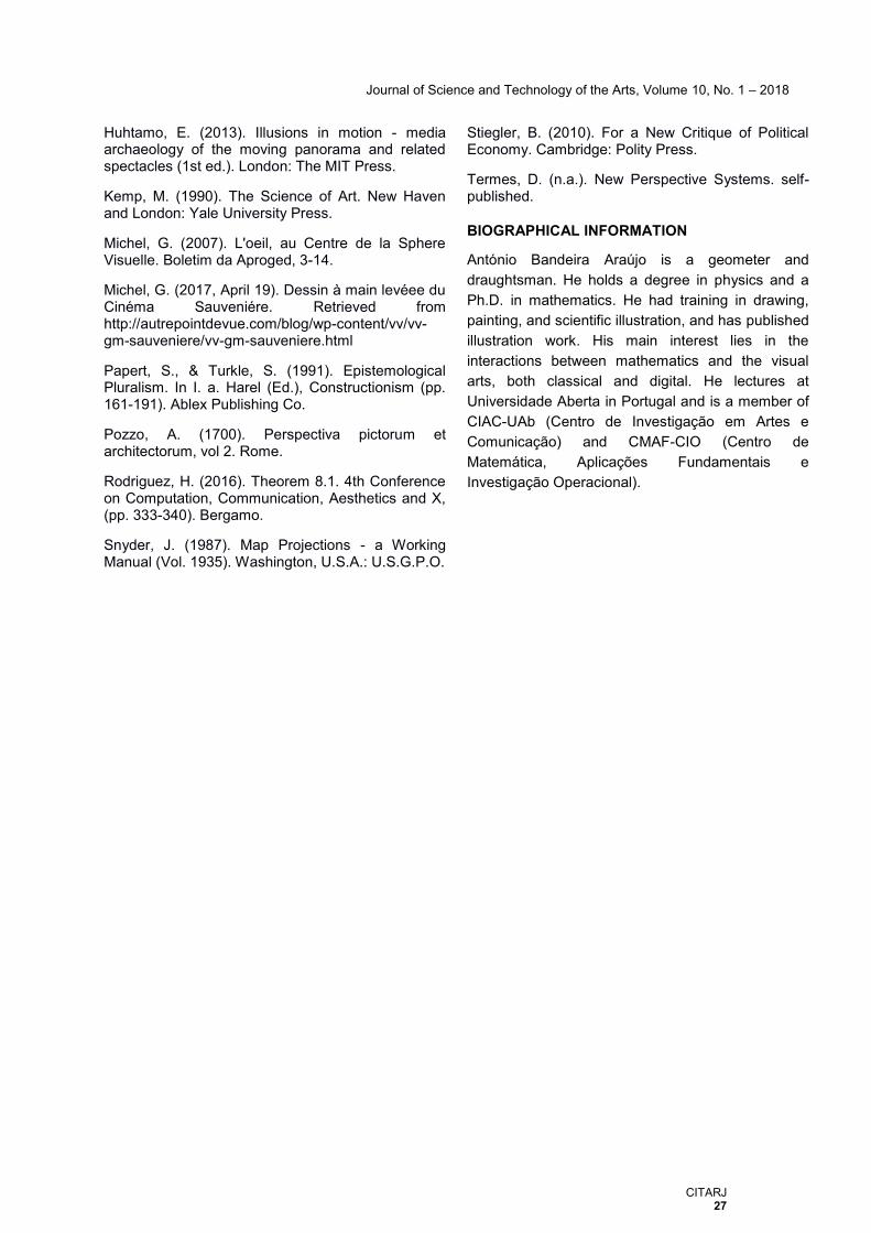
something you’d like to do while outdoor sketching.
There, you really want to grid. But our study of
symmetries has shown that the grid of horizontals
and verticals (Figure 4) has more to it than is
apparent at first: it is a plot of great circles, and this
can be used for a smarter kind of gridding, not
limited to drawing horizontals and verticals and
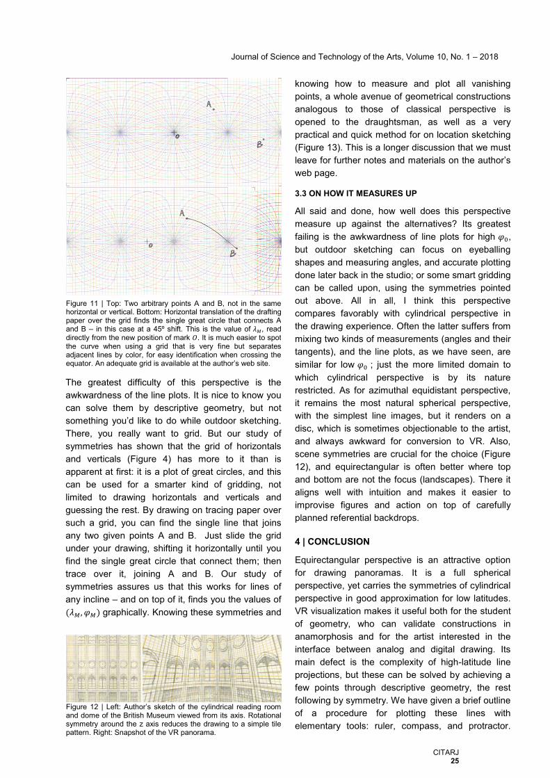
guessing the rest. By drawing on tracing paper over
such a grid, you can find the single line that joins
any two given points A and B. Just slide the grid
under your drawing, shifting it horizontally until you
find the single great circle that connect them; then
trace over it, joining A and B. Our study of
symmetries assures us that this works for lines of
any incline – and on top of it, finds you the values of
(𝜆𝑀, 𝜑𝑀) graphically. Knowing these symmetries and
knowing how to measure and plot all vanishing
points, a whole avenue of geometrical constructions
analogous to those of classical perspective is
opened to the draughtsman, as well as a very
practical and quick method for on location sketching
(Figure 13). This is a longer discussion that we must
leave for further notes and materials on the author’s
web page.
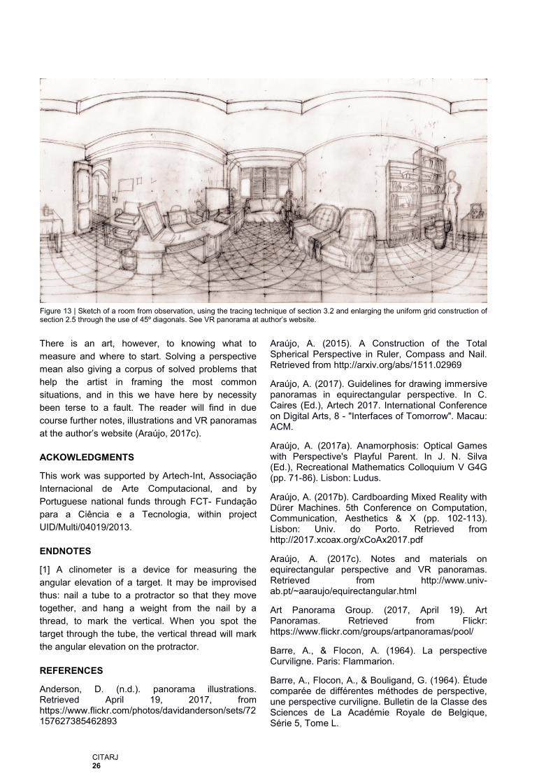
3.3 ON HOW IT MEASURES UP
All said and done, how well does this perspective
measure up against the alternatives? Its greatest
failing is the awkwardness of line plots for high 𝜑0,
but outdoor sketching can focus on eyeballing
shapes and measuring angles, and accurate plotting
done later back in the studio; or some smart gridding
can be called upon, using the symmetries pointed
out above. All in all, I think this perspective
compares favorably with cylindrical perspective in
the drawing experience. Often the latter suffers from
mixing two kinds of measurements (angles and their
tangents), and the line plots, as we have seen, are
similar for low 𝜑0 ; just the more limited domain to
which cylindrical perspective is by its nature
restricted. As for azimuthal equidistant perspective,
it remains the most natural spherical perspective,
with the simplest line images, but it renders on a
disc, which is sometimes objectionable to the artist,
and always awkward for conversion to VR. Also,
scene symmetries are crucial for the choice (Figure
12), and equirectangular is often better where top
and bottom are not the focus (landscapes). There it
aligns well with intuition and makes it easier to
improvise figures and action on top of carefully
planned referential backdrops.
4 | CONCLUSION
Equirectangular perspective is an attractive option
for drawing panoramas. It is a full spherical
perspective, yet carries the symmetries of cylindrical
perspective in good approximation for low latitudes.
VR visualization makes it useful both for the student
of geometry, who can validate constructions in
anamorphosis and for the artist interested in the
interface between analog and digital drawing. Its
main defect is the complexity of high-latitude line
projections, but these can be solved by achieving a
few points through descriptive geometry, the rest
following by symmetry. We have given a brief outline
of a procedure for plotting these lines with
elementary tools: ruler, compass, and protractor.
Figure 11 | Top: Two arbitrary points A and B, not in the same horizontal or vertical. Bottom: Horizontal translation of the drafting paper over the grid finds the single great circle that connects A and B – in this case at a 45º shift. This is the value of 𝜆𝑀, read directly from the new position of mark 𝑂. It is much easier to spot the curve when using a grid that is very fine but separates adjacent lines by color, for easy identification when crossing the equator. An adequate grid is available at the author’s web site.
Figure 12 | Left: Author’s sketch of the cylindrical reading room and dome of the British Museum viewed from its axis. Rotational symmetry around the z axis reduces the drawing to a simple tile pattern. Right: Snapshot of the VR panorama.
CITARJ 26
There is an art, however, to knowing what to
measure and where to start. Solving a perspective
mean also giving a corpus of solved problems that
help the artist in framing the most common
situations, and in this we have here by necessity
been terse to a fault. The reader will find in due
course further notes, illustrations and VR panoramas
at the author’s website (Araújo, 2017c).
ACKOWLEDGMENTS
This work was supported by Artech-Int, Associação
Internacional de Arte Computacional, and by
Portuguese national funds through FCT- Fundação
para a Ciência e a Tecnologia, within project
UID/Multi/04019/2013.
ENDNOTES
[1] A clinometer is a device for measuring the
angular elevation of a target. It may be improvised
thus: nail a tube to a protractor so that they move
together, and hang a weight from the nail by a
thread, to mark the vertical. When you spot the
target through the tube, the vertical thread will mark
the angular elevation on the protractor.
REFERENCES
Anderson, D. (n.d.). panorama illustrations. Retrieved April 19, 2017, from https://www.flickr.com/photos/davidanderson/sets/72157627385462893
Araújo, A. (2015). A Construction of the Total Spherical Perspective in Ruler, Compass and Nail. Retrieved from http://arxiv.org/abs/1511.02969
Araújo, A. (2017). Guidelines for drawing immersive panoramas in equirectangular perspective. In C. Caires (Ed.), Artech 2017. International Conference on Digital Arts, 8 - "Interfaces of Tomorrow". Macau: ACM.
Araújo, A. (2017a). Anamorphosis: Optical Games with Perspective's Playful Parent. In J. N. Silva (Ed.), Recreational Mathematics Colloquium V G4G (pp. 71-86). Lisbon: Ludus.
Araújo, A. (2017b). Cardboarding Mixed Reality with Dürer Machines. 5th Conference on Computation, Communication, Aesthetics & X (pp. 102-113). Lisbon: Univ. do Porto. Retrieved from http://2017.xcoax.org/xCoAx2017.pdf
Araújo, A. (2017c). Notes and materials on equirectangular perspective and VR panoramas. Retrieved from http://www.univ-ab.pt/~aaraujo/equirectangular.html
Art Panorama Group. (2017, April 19). Art Panoramas. Retrieved from Flickr: https://www.flickr.com/groups/artpanoramas/pool/
Barre, A., & Flocon, A. (1964). La perspective Curviligne. Paris: Flammarion.
Barre, A., Flocon, A., & Bouligand, G. (1964). Étude comparée de différentes méthodes de perspective, une perspective curviligne. Bulletin de la Classe des Sciences de La Académie Royale de Belgique, Série 5, Tome L.
Figure 13 | Sketch of a room from observation, using the tracing technique of section 3.2 and enlarging the uniform grid construction of section 2.5 through the use of 45º diagonals. See VR panorama at author’s website.
Journal of Science and Technology of the Arts, Volume 10, No. 1 – 2018
CITARJ 27
Huhtamo, E. (2013). Illusions in motion - media archaeology of the moving panorama and related spectacles (1st ed.). London: The MIT Press.
Kemp, M. (1990). The Science of Art. New Haven and London: Yale University Press.
Michel, G. (2007). L'oeil, au Centre de la Sphere Visuelle. Boletim da Aproged, 3-14.
Michel, G. (2017, April 19). Dessin à main levéee du Cinéma Sauveniére. Retrieved from http://autrepointdevue.com/blog/wp-content/vv/vv-gm-sauveniere/vv-gm-sauveniere.html
Papert, S., & Turkle, S. (1991). Epistemological Pluralism. In I. a. Harel (Ed.), Constructionism (pp. 161-191). Ablex Publishing Co.
Pozzo, A. (1700). Perspectiva pictorum et architectorum, vol 2. Rome.
Rodriguez, H. (2016). Theorem 8.1. 4th Conference on Computation, Communication, Aesthetics and X, (pp. 333-340). Bergamo.
Snyder, J. (1987). Map Projections - a Working Manual (Vol. 1935). Washington, U.S.A.: U.S.G.P.O.
Stiegler, B. (2010). For a New Critique of Political Economy. Cambridge: Polity Press.
Termes, D. (n.a.). New Perspective Systems. self-published.
BIOGRAPHICAL INFORMATION
António Bandeira Araújo is a geometer and
draughtsman. He holds a degree in physics and a
Ph.D. in mathematics. He had training in drawing,
painting, and scientific illustration, and has published
illustration work. His main interest lies in the
interactions between mathematics and the visual
arts, both classical and digital. He lectures at
Universidade Aberta in Portugal and is a member of
CIAC-UAb (Centro de Investigação em Artes e
Comunicação) and CMAF-CIO (Centro de
Matemática, Aplicações Fundamentais e
Investigação Operacional).
Recommended
![360° (Stereo) Panoramas - Christian Richardt · 2019-08-19 · 360° (Stereo) Panoramas 1. 360° panoramas –alignment + stitching [Brown & Lowe 2007] –parallax-aware stitching](https://img.pdfslide.net/doc/110x75/5edc94c9ad6a402d66674e5b/360-stereo-panoramas-christian-richardt-2019-08-19-360-stereo-panoramas.jpg)