DYNAMIC ANALYSIS OF A MONOSTABLE FLUID AMPLIFIER
By
HYO WHAN CHANG /I
Bachelor of Science in Engineering Seoul National University
Seoul, Korea 1968
Master of Science .State University of New York at Buffalo
Buffalo, New York 1972
Submitted to the Faculty of the Graduate College of the Oklahoma State University
in partial fulfillment of the requirements for the Degree of
DOCTOR OF PHILOSOPHY July, 1978

~t\ON~_ *-" /',,,
0 UNIVERSITY v
~ DYNAi'vliC ANALYSIS OF A MONOSTABLE FLUID AHPLIFIER
Thesis Approved:
Dean of the Graduate College
ii
ACKNOWLEDGMENTS
I wish to express my sincere appreciation and thanks to my thesis
adviser, Dr. Karl N. Reid, for his invaluable guidance and encouragement
throughout my doctoral program. Discussions with him have been most
valuable not only in the preparation of this thesis, but also in my pro
fessional development and growth.
I wish to thank Dr. William G. Tiederman, Dr. Jerald D. Parker, and
Dr. Robert J. Mulholland for serving on my thesis committee. Their valu
able advice and criticisms are greatly appreciated.
I wish to thank my colleagues and friends: especially Dr. Syed
Hamid for his encouragement and help; Vijay Maddali, Dave Smith, Steve
Mhoon, and John Perrault for their companionship.
I also wish to thank Ms. Charlene Fries for her expert typing of
this thesis.
Lastly, my wife, Young Mi, deserves special thanks for her patience
and sacrifices.
iii
TABLE OF CONTENTS
Chapter
I. INTRODUCTION
1.1 Background • • ••• 1.2 Objectives of Study •.•. 1.3 Thesis Outline • . • • •
II. LITERATURE SURVEY
2.1 Jet Reattachment Analysis 2.2 Switching Analysis .
III. ANALYTICAL HODELS
3.1 Steady-State Jet Reattachment Model 3.2 Dynamic Model •••••••.••
IV. EXPERIMENTAL APPARATUS AND PROCEDURE
4.1 Apparatus •••••.•••. 4.2 Instrumentation and Measurement Procedure
V. RESULTS AND DISCUSSION ••••
Page
1
1 12 13
15
15 21
27
28 45
80
80 87
91
5.1 Jet Spread Parameter • 91 5.2 Comparison of Steady-State Jet Reattachment
Model Predictions With Experimental Data . • . • . 92 5.3 Comparison of Dynamic Model Predictions With
Experimental Data . . • • • • • • • • • • 99 5.4 Experimental Data Repeatability •••••••••• 112 5.5 Effects of Geometric Variations on Switching
and Return Times • . . • • . • • 5.6 Limitation of the Model ••••
VI. SUMMARY, CONCLUSIONS, AND RECOMMENDATIONS
6.1 6.2 6.3
BIBLIOGRAPHY .
Sunun.ary . . . • . • . • • . . • • Conclusions . . • . • • • • • • • Recommendations for Future Study
iv
• 112 • . • • 127
• 132
• 132 • 135
. • • 136
• 138
Chapter Page
APPENDIX A - DRAWING OF TEST AMPLIFIER NOZZLE SECTION • 143
APPENDIX B - CONTROL NOZZLE DISCHARGE COEFFICIENT • • 145
APPENDIX C - COMPUTATION PROCEDURES AND SELECTED COMPUTER PROGRAM LISTINGS . . • • . • • • • • . • • • • • • • • 150
v
LIST OF TABLES
Table
I. Nominal Configuration •.•
II. Geometries of Test Models .
III. Definitions of Variables and Parameters
vi
Page
85
106
158
LIST OF FIGURES
Figure
1. Illustration of the Coanda Effect •.•
2. Simplified Representation of a Bistable Fluid Amplifier .
3. Simplified Representation of a Monostable Fluid Amplifier
4. Typical Static Switching Characteristics of WallAttachment Amplifiers . • • • . • • • • • •
5. Monostable Fluid Amplifier With an Input Vent Port
6. Effect of Connecting Transmission Line on the Switching Time of the Monostable Fluid Amplifier for Pte = 0.41 .•••
7. Effect of Connecting Transmission Line on the Return Time ·of the Monostable Fluid Amplifier for Pte = 0.41 .•••
8. Two Geometries Studied by Bourque and Newman
9. Bourque's Reattachment Model (With No Control Port)
10. Steady-State Jet Reattachment With Control Flow . . 11. Geometry for the Steady-State Jet Reattachment Model
12. Overall Steady-State Flow Model for a Monostable Fluid Amplifier • • • • . . • • .
13. Control Flow Passage Width
14. Geometry of Jet Centerline Curvature
. . . . .
. . . . . . . . .
Page
2
4
4
5
9
10
11
17
18
29
31
36
38
43
15. Flow Model for the Separation Bubble 47
16. Transition Between Phase I and Phase II . 48
17. Output Vent Flow Passage Width 49
18. Momentum Balance in the Vicinity of the Reattachment Point 55
19. Flow and Geometric Model for Unattached-Side Pressure •
20. Cross Section of Separation Bubble
vii
57
61

Figure Page
21. Geometry of Control and Output Channels • 62
22. Flow Model for Phase II 66
23. Bias Vent Flow Passage Width . . . . . . . . . . . . . 68
24. Geometry of the Attached Jet for Phase II • . . . . 74
25. Plan View of Large-Scale Test Amplifier . 81
26. Photograph of the Test Amplifier 82
27. Internal Geometry of the Test Amplifier • 84
28. Schematic of Experimental Apparatus . . • 86
29. Jet Centerline Axial Velocity Distributions in the Semi-Confined Jet (AR = 3.1) • • • • • • • • • • • • 93
30. Variation of Steady-State Reattachment Distance With Control Flow Rate for D1 = 0.5 and a1 = 15° . • • • • . . . • • . • • 95
31. Variation of Steady-State Reattachment Distance With Control Flow Rate for D1 = 1.0 and a1 = 15° • . . . • • • • • • • • . 96
32. Variation of Jet Deflection Angle With Control Flow Rate for D1 = 0.482 and a1 = 15° • . • • • . • • • • • • • 97
33. Variation of Jet Deflection Angle With Control Flow Rate 98
34. Variation of Switching Time With Control Pressure for the Monostable Fluid Amplifier With the Nominal Geometry • . . • 100
35. Variation of Return Time With Control Pressure for the Monostable Fluid Amplifier With the Nominal Geometry • • • • 102
36. Effect of Jet Spread Parameter ( ) Variation on the Switching Time for the Monostable Fluid Amplifier . • • • • • 104
37. Variation of Switching Time With Control Pressure for a Bistable Fluid Amplifier • • • . • • . • • • • • • • • 105
38. Variation of Switching Time With Control Pressure for a Bistable Fluid Amplifier • • • • • • • • • • • • 108
39. NOR Output Total Pressure Transient Response of the Monostable Fluid Amplifier . • • • • • • • 109
40. Predicted Effect of Control Input Pressure Shape on the OR Output Total Pressure Transient Response of the Monostable Fluid Amplifier . • • • • • • • • • • 111
viii
Figure Page
41. Variation of Switching and Return Times With Attachment Wall Offset • . . • • • . • • • • • • • • . • 114
42. Variation of Switching Time \Vith Opposite Wall Offset • • 115
43. Variation of Return Time With Opposite Wall Offset 116
44. Bias Vent Flow Passage Width • 118
45. Variation of Switching Time With Splitter Distance • • 119
46. Variation of Return Time With Splitter Distance • • 121
47. Critical Splitter Distance . 122
48. Effect of Bias Vent Width on the Switching Time . • 123
49. Variation of Return Time With Bias Vent Width . • • • 125
50. Variation of Switching and Return Times With Opposite Wall Angle • • . • • . • • • • • • • • • • • • . • • • 126
51. Variation of Switching and Return Times With Splitter Offset . . . . . . . . . . . . . . . 128
52. Effect of Output Loading on the Switching Time 129
53. Drawing of Test Amplifier Nozzle Section • 144
54. Control Nozzle Discharge Coefficient •• 149
55. Flow Diagram for OR Output Pressure Transient Response Prediction . . . . . . . . . . . . . . . . . . . . . . 153
ix
a c
a v
a w
A c
A v
A w
AR
b s
c
NOMENCLATURE
flow passage width (see Figure 13), in.
flow passage width (see Figure 16), in.
flow passage width (see Figure 19), in.
normalized flow passage width a (a /b ) c c s
normalized flow passage width a (a /b ) v v s
normalized flow passage width a (a /b ) w w s
supply nozzle aspect ratio (height to width)
bias vent width, in.
control nozzle width, in.
supply nozzle width, in.
NOR output vent width, in.
OR output vent width, in.
normalized bias vent width (bb/bs)
normalized control nozzle (b /b ) c s
normalized NOR output vent width (b 1 /h ) v s
normalized OR output
normalized bias vent
vent width (b 2/b ) v s
width (bb/bs)
normalized control nozzle width (b /b ) c s
normalized NOR output vent width (b 1/b ) v s
normalized OR output vent width (b 2/b ) v s
67/90
control nozzle discharge coefficient
supply nozzle discharge coefficient
X

d s
G
I c
I' c
I' ol
I' o2
J
J m
J s
splitter distance downstream of the supply nozzle exit, in.
attachment wall offset, in.
opposite wall offset, in.
splitter offset, in.
normalized splitter distance (d /b ) s s
normalized attachment wall offset (d1/bs)
normalized opposite wall offset (d2/bs)
normalized splitter offset (d3/bs)
distance (see Figure 11), in.
distance (see Figure 24), in.
normalized distance e1 (e1 /bs)
normalized distance e2 (e2/bs)
distance (see Figure 14), in.
normalized distance g (g/b ) s
control channel inertance (per unit depth), lbf sec2/in. 4
NOR output channel inertance (per unit depth), lbf sec2/in. 4
OR output channel inertance (per unit depth), lbf sec2/in. 4
dimensionless control channel inertance parameter
dimensionless NOR output channel inertance parameter
dimensionless OR output channel inertance parameter
supply jet momentum flux (per unit depth), lbf/in.
momentum flux (per unit depth) of the induced flow from the bias vent, lbf/in.
momentum flux (per unit depth) proceeding downstream along the wall (see Figure 18), lbf/in.
momentum flux (per unit depth) of the combined (supply and control) jet, lbf/in.
momentum flux (per unit depth) separated by the splitter, lbf/in.
xi

k
K
Re' c
Re s
scale factor in the entrainment streamline path equation
normalized scale factor (k/b ) s
minor loss coefficient
control channel length, in.
NOR output channel length, in.
OR output channel length, in.
normalized control channel length (i /b ) c s
normalized NOR output channel length (i 1 /b ) 0 s
normalized OR output channel length (i 2/b ) 0 s
control jet Reynolds number based on the control nozzle width
modified control jet Reynolds number defined in Equation (B.2)
supply jet Reynolds number based on the supply nozzle width
bias vent exit pressure, psig
pressure at section zl (see Figure 12), psig
pressure at section z2 (see Figure 13), psig
dynamic pressure at the inlet of the NOR output channel, psig
dynamic pressure at the inlet of the OR output channel, psig
total pressure at the exit of NOR output channel, psig
total pressure at the exit of OR output channel, psig
static return pressure (see Figure 4), psig
static switching pressure (see Figure 4), psig
total pressure at the inlet of the control channel, psig
separation bubble pressure, psig
average pressure in the unattached side of the jet, psig
average pressure in region 1 (see Figure 19), psig
average pressure in region 2 (see Figure 19), psig
pressure difference across the jet (p2 - pl), psig
xii

pcb
pdl
pd2
Pol
po2
p tc
normalized 1 2 pressure ph (pb/Zp Us)
1 2 normalized pressure PC (p /zP U ) c s 1 2 normalized pressure pcb (p cb/Zp Us)
normalized 1 2 pressure pdl (pd/2P Us)
normalized 1 2 pressure pd2 <Pd/zP us) 1 2 normalized pressure Pol (pol/Zp Us)
1 2 normalized pressure Po2 <PozlzP us)
normalized pressure pte ( /1 U2) pte zP s
1 2 normalized pressure pl (pl/Z PUs)
normalized 1 2 pressure p2 (PzlzP Us) 1 2 normalized pressure P2a (p2/z pUs)
normalized 1 2 pressure p2b (p2b/ZpUs)
volumetric flow rate in.2/sec
(per unit depth) through the bias vent,
volumetric in.2/sec
flow rate (per unit depth) of control jet,
volumetric flow rate (per unit depth) entrained by the convex side of the jet, in.2/sec
volumetric flow rate (per unit depth) entrained by the convex side of the jet (qe2 = qe3 + qe4), in.2/sec
volumetric flow rate (per unit depth) entrained from region 1 by the convex side of the jet (see Figure 10), in.2/sec
volumetric flow rate (per unit depth) entrained from region 2 by the convex side of the jet (see Figure 19), in.2/sec
volumetric flow rate (per unit depth) through the NOR output channel, in.2/sec
volumetric flow rate (per unit depth) through the OR output channel, in.2/sec
volumetric flow rate (per unit depth) leaving the separation bubble (see Figure 10), in.2/sec
volumetric flow rate (per unit depth) of supply jet, in. 2/sec
xiii
Qb
Qc
Qel
Qe2
Qe3
Qe4
Qol
Qo2
Qvl
Qv2
r
r c
r e
r es
R
R c
R e
R es
s
s e
volumetric flow rate (per unit depth) through the NOR output vent, in,2/sec
volumetric flow rate (per unit depth) through the OR output vent, in,2/sec
volumetric flow rate (per unit depth) through the flow passage in.2/sec width a (see Figure w 19),
normalized volumetric flow rate qb (qb/qs)
normalized volumetric flow rate qc (qc/qs)
normalized volumetric flow rate qel (qe/qs)
normalized volumetric flow rate qe2 (qe2/qs)
normalized volumetric flow rate qe3 (qe/qs)
normalized volumetric flow rate qe4 (qe4/qs)
normalized volumetric flow rate qol (qo/qs)
normalized volumetric flow rate qo2 (qo2/qs)
normalized volumetric flow rate qvl (qv/qs)
normalized volumetric flow rate qv2 (qvz!qs)
normalized volumetric flow rate qw (qw/qs)
geometric variable defined by Equation (3.2), in.
average radius of curvature of the jet centerline, in.
distance (see Figure 11), in.
radius of the circular arc which is tangent to the entrainment streamline at point A1 (see Figure 14), in.
normalized geometric variable r (r/b ) s
normalized average radius of curvature of the jet centerline curvature (r /b )
c s
normalized distance r (r /b ) e e s
normalized radius r (r /b ) es es s
distance along the jet centerline, in. ,......._
distance along the entrainment streamline A1E (see Figure 10), in.
xiv
s 0
s p
s s
s v
s w
s e
s 0
s p
s s
s v
s w
t
t' d
t . rJ.
t I • rl.
t s
,........,... distance along the jet centerline, c1F (see Figure 10), in.
distance from the "hypothetical nozzle" exit to the "virtual origin" of the jet, in.
,......... distance along the entrainment streamline, A1P (see Figure 14), in.
distance along the jet centerline from the hypothetical nozzle exit to the splitter point (see Figure 12), in.
distance along the jet centerline from the hypothetical nozzle exit to the output vent flow passage (see Figure 16a)
distance along the jet centerline from the hypothetical nozzle exit to the flow passage w1w2 (see Figure 19), in.
normalized distance s (s /b ) e e s
normalized distance s (s /b ) 0 0 s
normalized distance s (s /b ) p p s
normalized distance s (s /b ) s s s
normalized distance s (s /b ) v v s
normalized distance s (s /b ) w w s
time, sec
decay time of control input pressure signal to wall-attachment fluid amplifier (see Figure 7), sec
decay time of input pressure signal to the transmission line (see Figure 7), sec
pure sonic delay in the transmission (see Figures 6 and 7), sec
return time, sec
rise time of control input pressure signal to wall-attachment fluid amplifier (see Figure 6), sec
rise time of input pressure signal to the transmission line (see Figure 6), sec
switching time, sec
transport time (b /U ), sec s s
XV
T r
T s
u
,2 u
u c
u s
v
X e
X r
X e
X r
variable defined by Equation (3.6b)
variable defined by Equation (3.45)
velocity component parallel to jet centerline at any point in the jet, in./sec
mean square value of turbulent velocity fluctuations parallel to jet centerline, in.2/sec2
jet centerline axial velocity
mean velocity at the NOR output channel exit plane (q01/W01), in./sec
continuity averaged velocity at the supply nozzle exit plane, in./sec
separation bubble volume (per unit depth),
volume unit depth (see Figure 20), in. 2 per
volume unit depth (see Figure 20), in. 2 per
volume per unit depth (see Figure 20), in. 2
normalized separation bubble volume (v/b2) s
NOR output channel width, in.
OR output channel width, in.
normalized width w01 (w01/bs)
normalized width w01 (w02 /bs)
distance (see Figure 11), in.
reattachment distance (see Figure 10), in.
attachment wall length (see Figure 27), in.
opposite wall length (see Figure 27), in.
distance (see Figure 11), in.
distance (see Figure 11), in.
normalized distance X (x /b ) e e s
normalized distance X (x /b ) r r s
xvi
in. 2
y s
B
y
0 v
0 w
ll v
ll w
z;
normalized distance xvl (x /b ) v s
normalized distance xv2 (x 2/b ) v s
normalized distance xl (x/bs)
normalized distance x2 (x/bs)
distance normal to the jet centerline (see Figure 10),
distance (see Figure 10), in.
distance (see Figure 14), in.
distance (see Figure 10), in.
distance (see Figure 14), in.
normalized distance ye (y /b ) e s
normalized distance defined by Equation (3. 63)
normalized distance yp (yp/bs)
normalized distance yr (y/bs)
normalized distance ys (y /b ) s s
Greek Symbols
attachment wall angle, radian
opposite wall angle, radian
jet deflection angle, radian
jet reattachment angle, radian
jet half-width at s = s (see Figure 16a), in. v
jet half-width at s = s (see Figure 19), in. w
normalized width ll (ll /b ) v v s
normalized width ll (ll /b ) w w s
in.
angle between the entrainment streamline and r (see Figure 11), radian
angle z; at pointE (see Figure 11), radian
xvii
nl angle (see Figure 14), radian
n2 angle (see Figure 14), radian
a angle (see Figure 11), radian
a angle (see Figure 11), radian e
a angle (see Figure 14), radian p
.A parameter defined by Equation (3.46)
\) fluid kinematic viscosity, . 21 ~n. sec
~ angle (see Figure 16) , radian
p fluid density, 1bf sec2lin. 4
a jet spread parameter
T normalized time (U tlb ) s s
T normalized switching time t (t It ) s s s t
T normalized return time t (t It ) r r r t
xviii
CHAPTER I
INTRODUCTION
1.1 Background
The utilization of fluidic technology in industrial, military, and
medical control systems has increased substantially in the last several
1 y~ars [2] [11] [27]. The well-known advantages of fluidic devices are
insensitivity to hostile environments (e.g., high temperature, radiation
and vibration), simplicity, ruggedness, reliability, and low maintenance
cost.
Digital fluidic devices or "fluid amplifiers" which utilize the
"wall-attachment" phenomenon (called "wall-attachment fluid amplifiers")
are used to implement logic circuits for a broad range of applications.
As the application of digital fluid amplifiers in circuits requiring fast
operating speed has increased, it has become essential to consider the
dynamic behavior of the fluid amplifiers and connecting transmission
lines in the course of system design. The switching times2 of digital
fluid amplifiers often govern the operating speed of the associated logic
system.
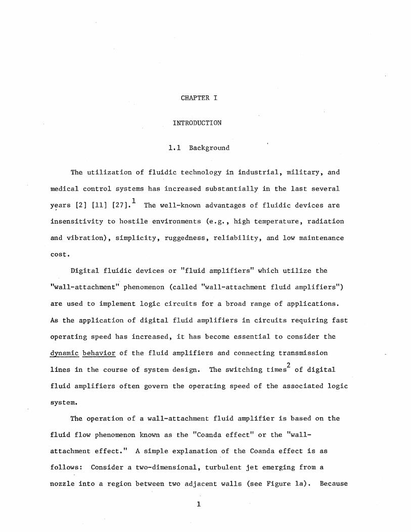
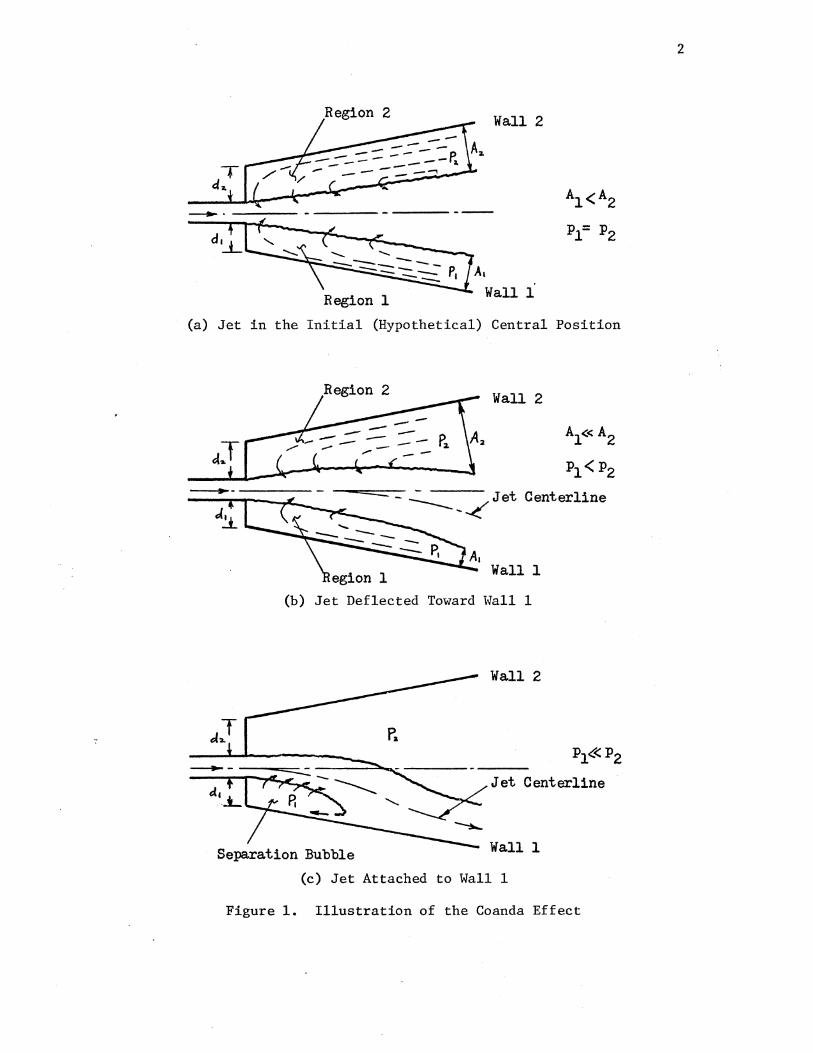
The operation of a wall-attachment fluid amplifier is based on the
fluid flow phenomenon known as the "Coanda effect" or the "wall-
attachment effect." A simple explanation of the Coanda effect is as
follows: Consider a two-dimensional, turbulent jet emerging from a
nozzle into a region between two adjacent walls (see Figure la). Because
1
Region 2 Wall 2
Region 1 Wall 1
(a) Jet in the Initial (Hypothetical) Central Position
Region 2 Wall 2
Al<< A2
pl <P2
- ..:____..c(Jet Centerline
Wall 1
(b) Jet Deflected Toward \vall 1
Separation Bubble
Wall 2
Pl<<P2
Jet Centerline
Wall 1
(c) Jet Attached to Wall 1
Figure 1. Illustration of the Coanda Effect
2

3
of the turbulent shearing action, the jet entrains fluid from the sur-
rounding regions [31]. If offset d1 of wall 1 is smaller than offset d2
of wall 2, the spacing A1 between wall 1 and the jet edge is smaller than
the spacing A2 between wall 2 and the jet edge (see Figure l(a)). Since
the jet entrains the same amount of fluid from region 1 and from region 2
(Figure l(a)), the average static pressure in region 1 becomes less than
that in region 2 to satisfy the jet entrainment. The resulting static
pressure difference (p2 - p1 ) causes the jet to deflect toward wall 1
(see Figure l(b)), which results in an even further increase in the pres-
sure difference. The only "stable" position for the jet is attachment to
wall 1; a low pressure cavity or bubble (called the separation bubble) is
formed as shown in Figure l(c). A state of equilibrium is reached when
the mass flow rate of fluid returned to the bubble is equal to the mass
flow rate of fluid entrained from it.
Simplified representations of wall-attachment fluid amplifiers are
shown in Figures 2 and 3. If the geometry of the wall-attachment ampli-
fier is symmetric (Figure 2), the supply jet attaches to either one of
the two walls due to the Coanda effect. This kind of wall-attachment
amplifier is called a bistable fluid amplifier. A typical static switch-
ing characteristic of a bistable amplifier is shown in Figure 4(a). If
the jet is initially attached to wall 1, the total pressure at output
port 1 (p01 ) is maximum and the total pressure at output port 2 (p02 ) is
minimum. The jet will switch to wall 2 and pressure p02 will be maximum
and pressure pol minimum if a control signal is app,lied at control port 1
which is equal to or greater than p • The jet will remain attached to s
wall 2 even if the control signal at port 1 is re1m0ved. Switching of the
jet from wall 2 to wall 1 requires the application of a positive pressure

Supply Port
Supply
Control Port 2
Output Vent Port 2
~ Output Port 2
Splitter
Output Port 1
~ Output Vent Port 1
Figure 2. Simplified Representation of a Bistable Fluid Amplifier
Bias Vent Port
OR Output Vent Port
~ OR Output
Port
Splitter Port ~----
ot,/ ~ NOR Output Vent Port
NOR Output Port
Figure 3. Simplified Representation of a Monostable Fluid Amplifier
4

max
min
max
min
Total Pressure at Output Port 2
Po2
0 ..
Control Pressure
(a) Typical Static Switching Characteristic of a Bistable Fluid Amplifier
Total Pressure at OR Output
0 Control Pressure
(b) Typical Static Switching Characteristic of a Monostable Fluid Amplifier
Figure 4. Typical Static Switching Characteristics of Wall-Attachment Amplifiers
5
signal at control port 2 which is equal to or greater than p in magnis
6
tude, or the application of a negative pressure signal at control port 1
equal to or less than p • r
If the geometry of the wall-attachment amplifier is asymmetric
(e.g., d1 < d2 , be< bb' a1 < a2 , and d3 # 0 in Figure 3), the supply
jet tends to attach to the "attachment wall" in the absence of a control
signal. This kind of wall-attachment amplifier is called a monostable
fluid amplifier. A typical static switching characteristic of a mono-
stable amplifier is shown in Figure 4(b). The jet is initially attached
to the "attachment wall" and the total pressure at NOR output port (p01)
is maximum, while the total pressure at OR output port (p02 ) is minimum.
The jet will switch to the "opposite wall" and pressure p02 will be maxi
mum and pressure p01 minimum, if a control signal is applied which is
equal to or greater than p • If this control signal is then reduced to s
a level equal to or less than p , the jet will switch back to the r
"attachment wall."
Output vents (see Figures 2 and 3) are provided in wall-attachment
amplifiers to avoid false switching due to a partial or complete block-
age of an output port.
The monostable amplifier is logically an OR/NOR device. It is a
fundamental building block of any logic circuit, since all other logic
functions (e.g., AND, NAND, FLIP-FLOP, etc.) can be generated by circuits
containing only OR/NOR elements. Nevertheless, no analytical studies and
only a few experimental studies have been done on the switching dynamics
of monostable fluid amplifiers, while there have been a large number of
analytical and experimental studies on the switching dynamics of bistable
fluid amplifiers.

7
It is known that a monostable fluid amplifier can be derived from a
bistable amplifier by minor geometric changes in the design. For example,
a bistable fluid amplifier can be made monostable by the following geo-
metric change(s) in the design (see Figure 3):
1. by making opposite wall offset d2 greater than attachment wall
offset d1 , or
2. by making bias vent width bb greater than control nozzle width
b , or c
3. by making opposite wall angle a2 greater than attachment wall
angle a1 , or
4. by combinations of the above changes.
But, how the above changes affect switching and return times3 and static
characteristics (e.g., static switching and return pressures, pressure
and flow gains, etc.) of a monostable fluid amplifier is not well under-
stood. For lack of an analytical model, monostable fluid amplifier de-
signs have been based primarily on trial-and-error procedures, with
design guides provided by experiments and very limited theories such as
a wall-attachment theory. The need for additional design information
was also suggested by Foster and Parker [22].
The switching times of digital fluid amplifiers are known to be
dependent on the control input pulse characteristics (i.e., input pulse
shape and magnitude). A pulse signal transmitted from the output of a
fluidic sensor or amplifier to the control input of a wall-attachment
fluid amplifier through a connecting transmission line usually experi-
ences a certain amount of pure time delay, attenuation and dispersion.
The change in pulse shape depends on the s~gnal pressure level, the input
characteristic of the driven amplifier, and the geometry of the connecting

8
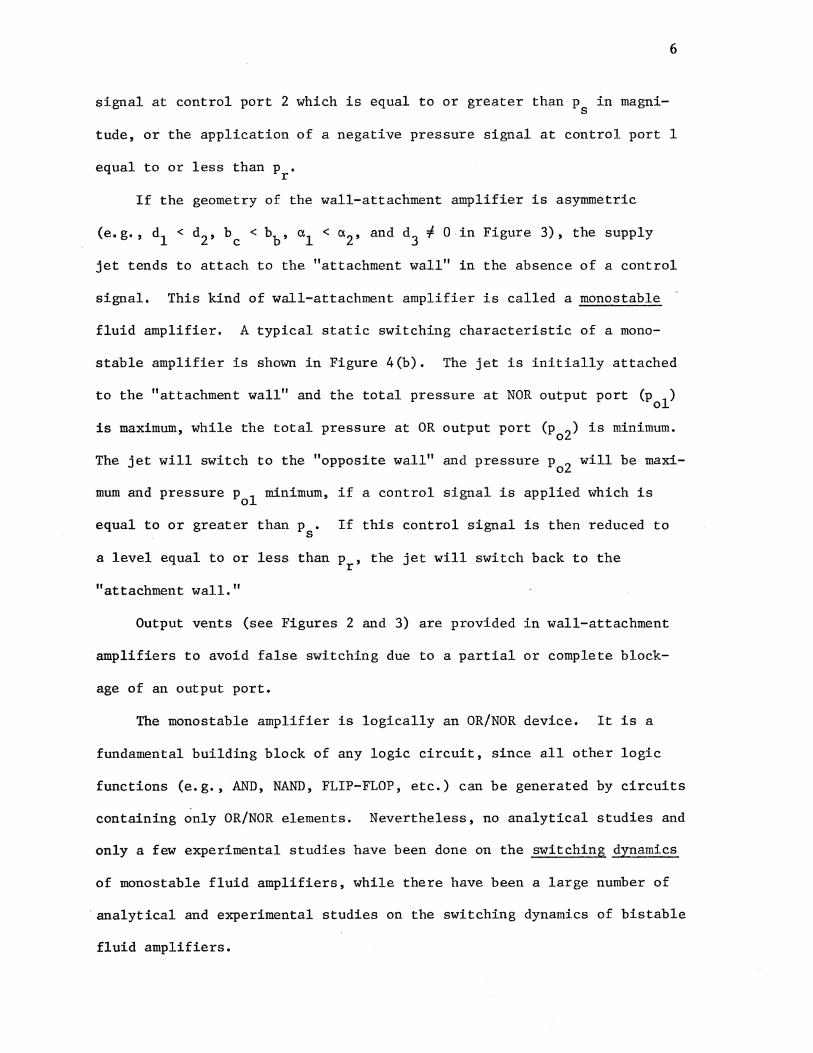
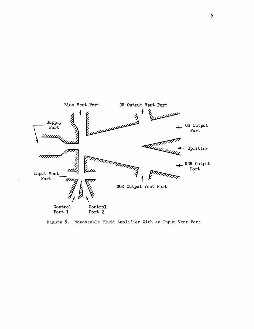
transmission line. Moreover, an input vent port (see Figure 5) provided
for control input signal isolation in a wall-attachment amplifier may re-
sult in significant input pulse signal attenuation and dispersion.
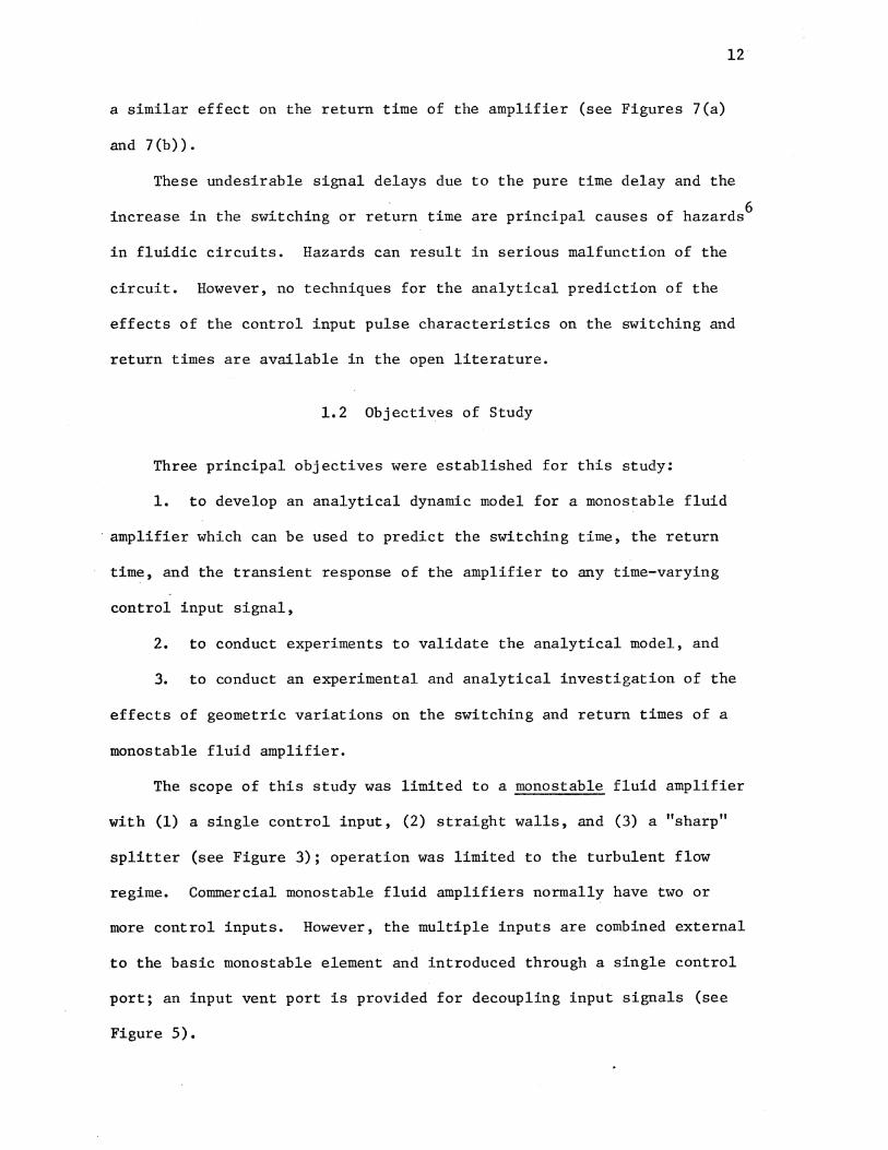
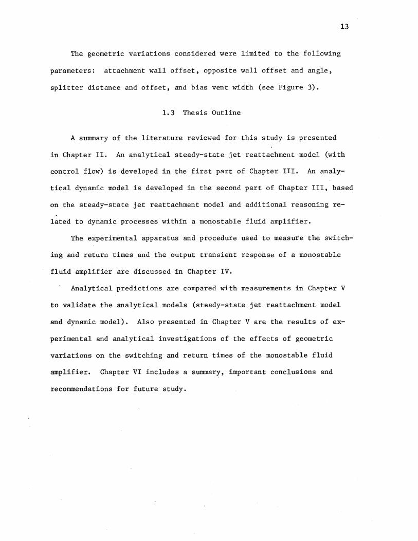
Figures 6 and 7 show the effects of a connecting transmission line
on the switching and return times of the monostable fluid amplifier used
in the present study. A solid line in the output velocity trace indi-
cates the measured result; a dashed line indicates the actual magnitude
and sign of the velocity where there is a flow reversal. That is, the
hot-wire probe used in the measurements is not directional sensitive. A
42 foot long (1/4 inch inside diameter and 3/8 inch outside diameter)
flexible plastic tubing served as a connecting transmission line between
the control pressure source and the control chamber of the test amplifier
for the measurements in Figures 6(b) and 7(b). "Step-like" pressure
pulses were generated at the control port of the amplifier (Figures 6(a)
and 7(a)) and at the inlet of the transmission line (Figures 6(b) and
7(b) by means of a solenoid valve connected to a constant-pressure source.
When the transmission line was connected to the control part of the ampli-
fier, the magnitude of the pressure pulse at the control port was kept
the same as that without a transmission line by adjusting the magnitude
of the pressure pulse at the inlet of the transmission line.
The transmission line caused the pure time delay tt and long rise
4 time of the control input pressure to the amplifier. Due to the in-
creased rise time in the control input pressure to the amplifier, the
switching time5 of the amplifier with the transmission line was approxi-
mately five times longer than that of the amplifier without the trans-
mission line (see Figures 6(a) and 6(b)). The transmission line caused
Bias Vent Port
Supply \ Port
\~~~-'-.£.~&.1
Input Vent
Port _1A~ Control Port 1
Control Port 2
OR Output Vent Port
·~ OR Output
Port
..c- NOR Output Port
NOR Output Vent Port
Figure 5. Monostable Fluid Amplifier With an Input Vent Port
9

" -1!.- t ri .. I
I I I I I I I I I I I '
. --r I Actual~ --l ts ~.-
I •. ~· . . ..
(a) W[ith<?ut:Transmissibn lSine
I I ~ t,.';
I. I I I
I
!..-
.. -----~ .. CJ
--- -·""":"" ___ _ I-- ts
(b) With Transmission Line
:.A:.
10
Control input pressure to amplifier
OR output velocity
t .= ri
2.5 ms
= 19.3 ms .t s
Input pressure to transmission line
Control input pressure to amplifier (B < A due to attenu-ation)
OR output velocity
t' . = 32.8 ms rJ. tQ, = 38.9 ms
t = 49.2 ms ri ts = 94.6 ms
Figure 6. Effect of Connecting Transmission Line on the Switching Time of the Monostable Fluid Amplifier for P = 0.41 tc

·. 4fl~¢11)1l!ll
I' -l;_tJ .. I .
I . I
I .... I
. I
Measured\ :
,_----c- I
Actual·/ __j tr I-
--·-4··--~ ·---------·!--· ----- ---- --· -~--- ..
-- - . ~- . . .. -- .. ----- -
(a) Without :Tr1uismission :Line!
s
I
-I t.e :_ tJ I I I
.I .... I.
I I ___ , ____ _ I
·--'. tr I I • t...-
' - ---------- ------~1----- ---L-- -
...
11
Control input pressure to amplifier
NOR output velocity
td = 1.5 ms
tt = 29.2 ms
Input·pressure to transmission line
Control input pressure to amplifier (B < A due to attenuation}
NOR output velocity
t' = 99.8 ms d
t = 37.9 ms
td = 130.6 ms
t = 102.4 ms J r
Figure 7. Effect of Connecting Transmission Line on the Return Time of the Monostable Fluid Amplifier for p = 0.41 tc
12
a similar effect on the return time of the amplifier (see Figures 7(a)
and 7 (b)).
These undesirable signal delays due to the pure time delay and the
increase in the switching or return time are principal causes of hazards6
in fluidic circuits. Hazards can result in serious malfunction of the
circuit. However, no techniques for the analytical prediction of the
effects of the control input pulse characteristics on the switching and
return times are available in the open literature.
1.2 Objectives of Study
Three principal objectives were established for this study:
1. to develop an analytical dynamic model for a monostable fluid
amplifier which can be used to predict the switching time, the return
time, and the transient response of the amplifier to any time-varying
control input signal,
2. to conduct experiments to validate the analytical model, and
3. to conduct an experimental and analytical investigation of the
effects of geometric variations on the switching and return times of a
monostable fluid amplifier.
The scope of this study was limited to a monostable fluid amplifier
with (1) a single control input, (2) straight walls, and (3) a "sharp"
splitter (see Figure 3); operation was limited to the turbulent flow
regime. Commercial monostable fluid amplifiers normally have two or
more control inputs. However, the multiple inputs are combined external
to the basic monostable element and introduced through a single control
port; an input vent port is provided for decoupling input signals (see
Figure 5).
The geometric variations considered were limited to the following
parameters: attachment wall offset, opposite wall offset and angle,
splitter distance and offset, and bias vent width (see Figure 3).
1.3 Thesis Outline
A summary of the literature reviewed for this study is presented
13
in Chapter II. An analytical steady-state jet reattachment model (with
control flow) is developed in the first part of Chapter III. An analy
tical dynamic model is developed in the second part of Chapter III, based
on the steady-state jet reattachment model and additional reasoning re
lated to dynamic processes within a monostable fluid amplifier.
The experimental apparatus and procedure used to measure the switch
ing and return times and the output transient response of a monostable
fluid amplifier are discussed in Chapter IV.
Analytical predictions are compared with measurements in Chapter V
to validate the analytical models (steady-state jet reattachment model
and dynamic model). Also presented in Chapter V are the results of ex
perimental and analytical investigations of the effects of geometric
variations on the switching and return times of the monostable fluid
amplifier. Chapter VI includes a summary, important conclusions and
recommendations for future study.

ENDNOTES
1Numbers in brackets designate references in the Bibliography.
2s . h' . WJ.tc J.ng tJ.me control input signal until the associated its final value.
is defined as the time elapsed is applied to the control port output pressure (or flow rate)
from the instant the (see Figures 2 and 3) reaches 95 percent of
3switching times in the monostable amplifier consist of the switching time from the NOR to OR output and the switching time from the OR to NOR output (see Figure 3). In this study the former is called "switching time" and the latter "return time." The return time is defined in a manner similar to that of the switching time.
4The rise (or decay) time is defined as the time elapsed from the first discernible change in the control input pressure (within 5 percent) until the pressure reaches 5 percent of its final value. The control input pressure was slightly increased after the jet switched to the opposite wall. Therefore, the steady-state value of the control input pressure just before switching was taken as the final value.
5The switching (or return) time is defined in this measurement as the time elapsed from the first discernible change in the control input pressure (within 5 percent) until the associated output velocity reaches 95 percent of its final value.
6The various types of hazards in fluidic circuits are discussed by Parker and Jones [49].
14
CHAPTER II
LITERATURE SURVEY
Dynamic analysis of a monostable fluid amplifier requires an under
standing of both steady-state jet reattachment phenomena and dynamic flow
processes inside the wall-attachment device. Previous work on these two
topics is surveyed in this chapter.
In brief, a survey of the literature reveals the following:
1. No analytical studies on the dynamic behavior of a monostable
fluid amplifier have been reported in the open literature.
2. Although extensive analytical and experimental work has been
done on the basic jet reattachment phenomena in wall-attachment devices,
no analytical model has been successful in accurately predicting the
position of the jet reattachment in the presence of control flow.
3. No comprehensive experimental results have been reported in
the open literature concerning the effects of the geometric variations
on the switching and return times of a monostable fluid amplifier.
2.1 Jet Reattachment Analysis
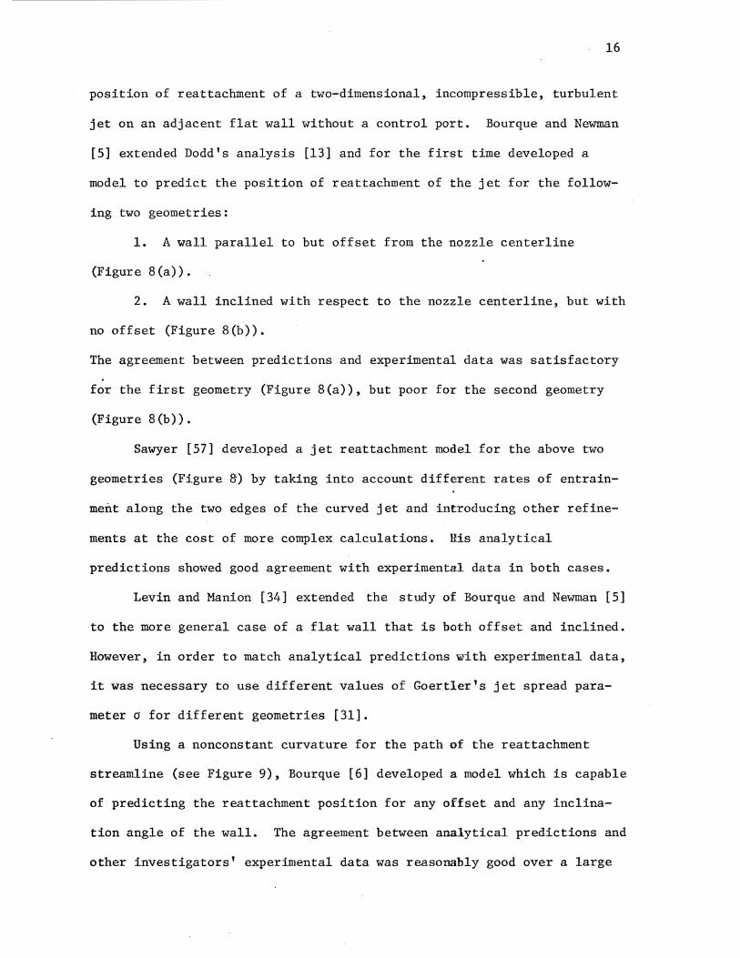
Studies on jet reattachment have been conducted for cases with and
without a control port (see Figures 2 and 9).
2.1.1 Jet Reattachment With No Control Port
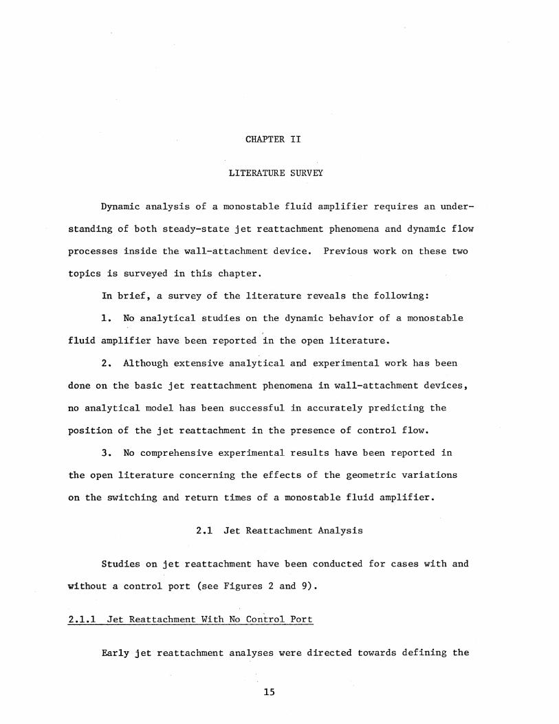
Early jet reattachment analyses were directed towards defining the
15
16
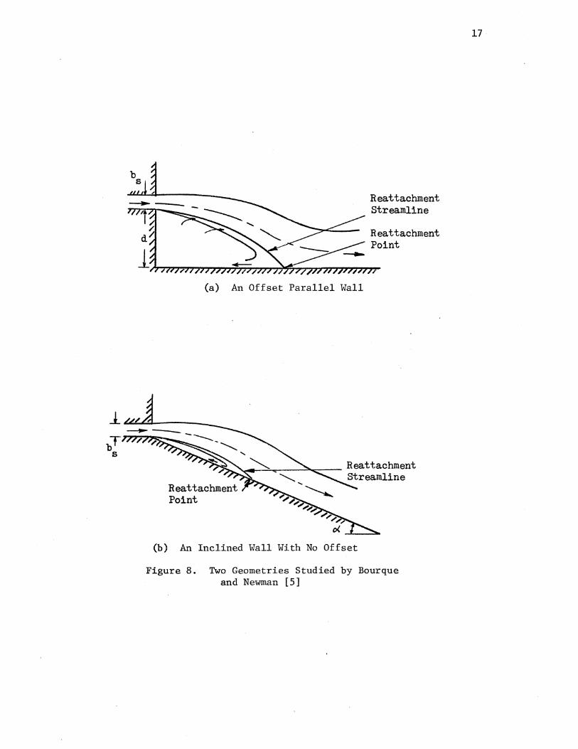
(a) An Offset Parallel Wall
Reattachment Point
(b) An Inclined Wall With No Offset
Reattachment Streamline
Figure 8. Two Geometries Studied by Bourque and Newman [5]
17
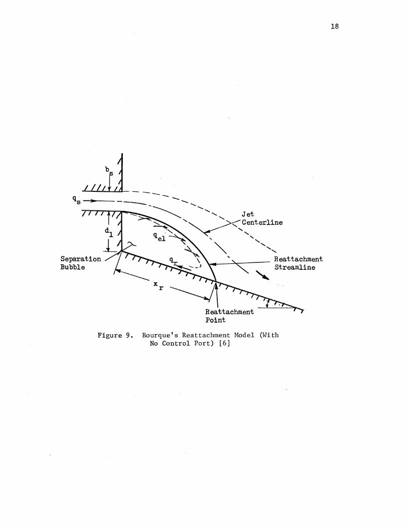
-"-""-'-"'--'-"-- - - -qs --il---
Separation Bubble
-
X r
Reattachment Point
Figure 9. Bourque's Reattachment Model (With No Control Port) [6]
18
19
range of wall offsets and angles, using a constant value of the jet spread
parameter (i.e., a= 10.5).
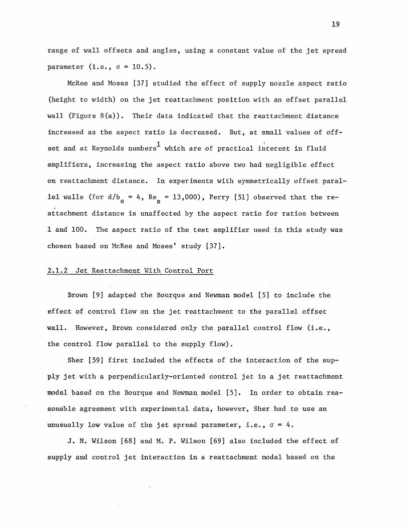
McRee and Moses [37] studied the effect of supply nozzle aspect ratio
(height to width) on the jet reattachment position with an offset parallel
wall (Figure S(a)). Their data indicated that the reattachment distance
increased as the aspect ratio is decreased. But, at small values of off
set and at Reynolds numbers1 which are of practical interest in fluid
amplifiers, increasing the aspect ratio above two had negligible effect
on reattachment distance. In experiments with symmetrically offset paral-
lel walls (for d/b = 4, Re = 13,000), Perry [51] observed that there-s s
attachment distance is unaffected by the aspect ratio for ratios between
1 and 100. The aspect ratio of the test amplifier used in this study was
chosen based on McRee and Moses' study [37].
2.1.2 Jet Reattachment With Control Port
Brown [9] adapted the Bourque and Newman model [5] to include the
effect of control flow on the jet reattachment to the parallel offset
wall. However, Brown considered only the parallel control flow (i.e.,
the control flow parallel to the supply flow).
Sher [59] first included the effects of the interaction of the sup-
ply jet with a perpendicularly-oriented control jet in a jet reattachment
model based on the Bourque and Newman model [5]. In order to obtain rea-
sonable agreement with experimental data, however, Sher had to use an
unusually low value of the jet spread parameter, i.e., a= 4.
J. N. Wilson [68] and M. P. Wilson [69] also included the effect of
supply and control jet interaction in a reattachment model based on the
20
Bourque and Newman model [5]. Neither of their models was in good agree-
ment with experimental data.
Using a modified Goertler's free jet model (including a potential
core and nonsymmetric velocity profile), Kimura and Mitsuoka [30] devel-
oped a complex model where two different mechanisms of reattachment were
taken into account: (1) reattachment in the zone of established flow,
and (2) reattachment in the zone of flow establishment. In spite of its
complexity, the model was not in good agreement with experimental data.
Moreover, it was necessary to use different values of the jet spread
parameter a for different geometries. However, their experimental data
[30] are believed to be the best in thoroughness among that available
in the open literature. Therefore, their experimental data are used in
this thesis for the validation of the analytical steady-state jet re-
attachment model.
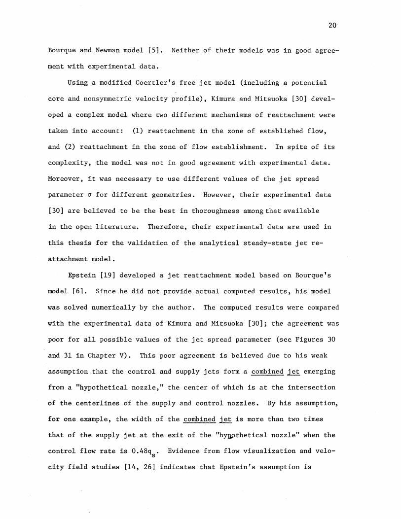
Epstein [19] developed a jet reattachment model based on Bourque's
model [6]. Since he did not provide actual computed results, his model
was solved numerically by the author. The computed results were compared
with the experimental data of Kimura and Mitsuoka [30]; the agreement was
poor for all possible values of the jet spread parameter (see Figures 30
and 31 in Chapter V). This poor agreement is believed due to his weak
assumption that the control and supply jets form a combined jet emerging
from a "hypothetical nozzle," the center of which is at the intersection
of the centerlines of the supply and control nozzles. By his assumption,
for one example, the width of the combined jet is more than two times
that of the supply jet at the exit of the "hyaothetical nozzle" when the
control flow rate is 0.48q • Evidence from flow visualization and velos
city field studies [14, 26] indicates that Epstein's assumption is
21
unreasonable. In this thesis, Epstein's "hypothetical nozzle" concept
with modification (i.e., the deflected supply jet emerges from the "hypo
thetical nozzle" without mixing with the control jet) is used in the
development of an improved steady-state jet reattachment model. Certain
geometric relations used in Epstein's model are also utilized in this
thesis (see Chapter III for more details).
Olson and Stoeffler [45] and Brown and Belen [8] have developed
semi-empirical models to predict the effect of control flow on the re
attachment location. Experimental studies in this area have been done
by Foster and Jones [21], Olsen and Chin [43], and Wada and Shimizu [62].
In summary, no analytical model has been successful in accurately
predicting the position of the jet reattachment in the presence of con
trol flow. An improved steady-state jet reattachment model is developed
in this thesis based on a modification of Bourque's model [6] to include
the effect of control flow and the opposite wall.
2.2 Switching Analysis
2.2.1 Switching Analysis of the Bistable
Amplifier
Due to the complexity of the fluid dynamic phenomena involved in
the transient switching process, and the many geometric and fluid flow
parameters affecting the switching, most of the early work in this area
has been experimental.
Warren [32, 64] made qualitative experimental observations concern
ing the effects of changing parameters on the characteristics of the bi
stable amplifier, and classified the switching processes into three types

22
as follows: (1) "terminated-wall" (or "end-wall"), (2) "contacting-both
walls" (or "opposite-wall"), and (3) "splitter switching." Comparin
et al. [10] first measured the switching time by using a high speed motion
picture camera. Keto [29] and Sarpkaya [54] conducted qualitative studies
on the transient switching behavior of the bistable amplifier. Savkar
et al. [55] studied the effect of varying geometric parameters on the
switching times of a large scale test model of a bistable amplifier; but,
these data are not of value in the present study, since the geometry of
the model was somewhat different than that of the typical bistable ampli
fier.
Semi-empirical models for the separation time2 of a jet in a single
wall amplifier were developed by Johnston [28], Muller [41, 42], Olson
and Stoeffler [44], and J. N. Wilson [68].
Lush [35, 36] first developed a theoretical model to predict switch
ing times for "end-wall type switching" in a bistable amplifier, which is
based on the work done by Sawyer [56, 57] and Bourque and Newman [5]. His
theoretically predicted switching times were about one-half the measured
values. However, his thorough experimental investigation of the switching
mechanism in a large-scale model provides a good qualitative description
of the physical flow phenomena involved in the transient switching process
of a monostable fluid amplifier. Lush's [36] experimental data on the jet
deflection angle are the only comprehensive data reported in the open
literature for the wall-attachment amplifier; therefore, his data are used
in this thesis for comparison with analytically predicted jet deflection
angles. Also, his experimental data [36] on the switching time of a bi
stable fluid amplifier are used in this thesis for the validation of the
analytical dynamic model of a monostable fluid amplifier.
23
Epstein [19] also developed a theoretical model for the "end-wall
type switching" process, which is based on Bourque's theory [6]. Employ
ing an unusually large value of the jet spread parameter (cr = 31.5),
Epstein obtained good agreement with Lush's experimental data [35, 36].
As remarked by Epstein [19], however, the most serious limitation of his
theory is the dependence on experiment for a determination of a for each
geometrical condition of interest. As mentioned in section 2.1.2, his
"hypothetical nozzle" concept with modification and certain geometric
relations used in his model are utilized in this thesis in the dynamic
modeling of a monostable fluid amplifier, too.
Ozgu and Stenning [46, 47] conducted a theoretical study on the
"opposite-wall type switching" process using Simson's jet profile [60].
By including unsteady flow effects at the reattachment point on the flow
rate balance in the separation bubble, they obtained good agreement with
experimental data. Even though Simson's jet profile fits the measured
velocity profile data better than Goertler's jet profile [31, 58], espe
cially in the zone of flow establishment, Ozgu and Stenning obtained
quite similar results for the switching time when they used Goertler's
profile instead of Simson's profile. Since a monostable fluid amplifier
usually has a realtively large opposite wall offset, their model [46]
cannot be applicable to the dynamic modeling of the monostable amplifier.
However, their study [46, 47] provides justification for using Goertler's
profile in the dynamic modeling of a monostable amplifier.
Williams and Colborne [67] analyzed the splitter switching process
using Simson's profile. They considered only a sharp splitter in the
model.

24
A common limitation of the four analytical models mentioned above
(Lush, Epstein, Ozgu and Stenning, Williams and Colborne) is that the
models are applicable only to compute the switching time of the bistable
amplifier for a given "step-type" control input signal. Horeover, only
one of the three possible switching processes [32, 64] was considered in
each model. In an actual device, however, more than one type of switch-
ing process could be present, simultaneously. In this thesis, an analy-
tical dynamic model is developed for a monostable fluid amplifier, which
includes all three types of switching processes implicitly and considers
a time-varying control input signal. Therefore, the four models mentioned
above cannot be directly used in this thesis.
Goto and Drzewiecki [23] developed a dynamic model of the bistable
amplifier which allowed consideration of time-varying control input sig-
nals. They treated each channel (control, output vent, and output chan-
nels) as lumped-parameter lines and also included the effect of the
momentum "peeling off" from the jet by the splitter in their model, which
is based on the Bourque and Newman model [5]. Goto and Drzewiecki's
model was not in good agreement with the experimental data, especially
3 for cases where the "inactive control" port was open to ambient pres-
sure. However, Goto and Drzewiecki's treatment of the output channel in-
ertia and splitter effects and certain numerical computation procedures
used for their analytical predictions can be used in the present study
(see Chapter III for more details).
2.2.2 Switching Analysis of the Monostable
Amplifier
A difference between the switching time from the NOR to OR output
4 and the switching time from the OR to NOR output in the monostable
amplifier was first observed by Steptoe [61].
Foster and Carley [20] conducted an experimental study of the
effects of supply pressure, control flow, 5 the rise and decay times of
the control flow pulse and output loading on the switching times for a
particular monostable and a particular bistable fluid amplifier. How-
25
ever, the data presented by Foster and Carley are of qualitative interest
only and cannot be used in the present study for comparison, since no in-
formation about the dimensions of the amplifiers were reported.
Ozgu and Stenning [48] conducted a limited experimental study of the
effects of geometric variations (opposite-wall offset, splitter offset,
and attachment wall shape only), supply pressure, control flow, and output
loading on the switching and return times of the monostable amplifier,
using a special design large-scale test model. Since the geometry of the
test model used in their study is quite different from that of the typical
monostable fluid amplifier (i.e., no bias vent and no output vent were
provided in the opposite wall, and the attachment wall offset was slightly
. 6) h d db 0 d s . f 1. . negat1ve , t e ata presente y zgu an tenn1ng are o qua 1tat1ve
interest only and not used in the present study for comparison.
1
ENDNOTES
Based on the nozzle width: Re s
U b /v. s s
2The separation time is defined as the time elapsed from the moment when control input is applied until the jet is released from the wall.
3 Control port 2 was called an "inactive control" port by Goto and Drzewiecki [23] when a control input signal is applied to control port 1 (see Figure 2).
4The switching time from the NOR to OR output and the switching time from the OR to NOR output were called "switch on delay" and "switch off delay," respectively, by Steptoe [61].
5some investigators, including the author, use control pressure as the independent variable rather than control flow.
6The attachment wall offset is defined, in this study, as the distance d1 shown in Figure 11. With this definition, the attachment wall offset of the test model used by Ozgu and Stenning [48] was d1 = -0.143bs.
26
CHAPTER III
ANALYTICAL HODELS
This chapter presents the development of an analytical model which
predicts the steady-state jet reattachment position of a two-dimensional
turbulent jet to an offset, inclined wall in the presence of control
flow. Bourque's jet reattachment model [6] is used with necessary modi-
fications to include the effects of control flow and the opposite wall.
This chapter also presents the development of an analytical dynamic
model which predicts the switching time, the return time, and the transi-
ent response of a monostable fluid amplifier to any time-varying input
signal. The steady-state jet reattachment model developed in the first
part of this chapter is extended to include dynamic flow processes in-
side the monostable fluid amplifier.
All variables in capital letters are dimensionless. Variables with
the dimension of length are normalized with respect to supply nozzle
width b . Variables with the dimensions of area and volume are normals
2 ized with respect to b and b , respectively, since these variables are s s
defined per unit depth in the present model. Pressures are normalized
with respect to supply jet dynamic pressure~ pU!, and flow rates are
normalized with respect to the supply flow rate per unit depth q . s
Times are normalized with respect to the transport time t = b /U , t s s
i.e., the time required a fluid particle moving at the supply nozzle
27
28
exit velocity U (continuity averaged) to travel a distance of one sups
ply nozzle width.
3.1 Steady-State Jet Reattachment Model
3.1.1 Assumptions
The following assumptions are made for the mathematical formulation
of the steady-state reattachment model:
1. The jet flow is everywhere two-dimensional and incompressible.
2. Momentum interaction between the control and supply jets takes
place in control volume 1 shown in Figure 10; consequently, the supply
jet is deflected (angle 8 with respect to supply nozzle centerline).
It is assumed that the deflected jet emerges from a "hypothetical noz-
zle" of width bs' the exit of which is located at line A1A2 in Figure
10. 1
3. The velocity profiles at the exits of the control, supply and
hypothetical nozzles are uniform.
4. The supply jet velocity profile is describable by Goertler's
turbulent-jet profile [31] and is not affected by the presence of the
attachment wall. That is,
1,
3Ja ' 2
(s + s )] 0
sech2 ( cry ) s + s
0
(3.1)
2 where J is the momentum flux per unit depth (J = pb U ) , s is the dis
s s 0
tance from the "hypothetical nozzle" exit to the "virtual origin" of
the jet, and a is the jet spread parameter.
5. The static pressure and wall-shear forces acting on control
volume 2 in the vicinity of the reattachment point (Figure 10) are

Volume 1
q ~ . \ -S I.J., -----; I , ) j 7-At I
Separation 'I! f ~ Bubble
Reattachment Streamline
Entrainment Streamline
Jet Centerline
I I I I
1'--.. Jd S , I
I
Volume 2
Attachment Wall
Figure 10. Steady-State Jet Reattachment With Control Flow
('..;) \.0

30
negligible compared to the momentum flux of the jet. That is, in the
vicinity of the reattachment point, momentum is conserved.
6. The path of the entrainment streamline2 can be represented by
the equation
r = k . (-e) SJ.n c
(3.2)
where k is a scale factor, 8 is defined in Figure 11, and c 67 - 90 • (For
derivation of this equation, see Reference [6].)
7. Flow entrainment by the concave side of the jet ceases where
the extended entrainment streamline intersects the wall (i.e., at point
E in Figure 10).
8. The distance measured along the entrainment streamline is
approximately equal to the distance measured along the jet centerline.
9. The angle included between the extended jet centerline and the
wall is approximately the same as the one included between the extended
entrainment streamline and the wall (yin Figure 10).
10. The rate of fluid entrainment is the same on both sides of the
. 4 Jet.
11. The supply and control jets retain their identity (i.e., there
is no mixing of the jets) within control volume 1 in Figure 10. 5
12. The net pressure force acting in the longitudinal direction
(i.e., parallel to the supply nozzle centerline) on control volume 1 in
Figure 10 is negligible compared to the supply jet dynamic pressure.
13. The effect of the bias vent flow momentum flux on the jet de-
flection is negligible; the bias vent flow is "naturally" induced by the
low pressure in the. region between the jet edge and the opposite wall.

Entrainment Streamline
Figure 11. Geometry for the Steady-State Jet Reattachment Model
31
32
Assumptions 1, 3-5, 8-10, and 12 are either identical to or consistent
with those made by Bourque [6] and Epstein [19].
The major differences between the present model and Epstein's
steady-state reattachment model are: (1) in the width of the hypotheti-
cal nozzle, (2) in the definition of the separation bubble boundary, and
6 (3) in the calculation of the jet deflection angle.
Based on the assumptions mentioned above, the steady-state jet re-
attachment model is formulated as follmvs:
1. Basic equations (continuity, momentum, jet deflection) and geo-
metric relations are written.
2. Each equation is normalized with respect to the associated
variables.
3. A numerical computation procedure is established for the solu-
tion of the set of normalized equations.
3.1.2 Continuity Equation
The separation bubble is defined as the cavity enclosed between the ,--....
entrainment streamline A1E, attachment wall and lines IG, GH, and HA1
(see Figure 10). The flow balance in the separation bubble in the
steady state is
0 = q q c - out (3.3)
and
(3.3a)
where qel is the flow rate entrained by the concave side of the jet.
Equations (3.3) and (3.3a), when combined and normalized, yield
33
(3.4)
Referring to Figure 10 and assumptions 4, 7 and 8, the entrained
flow rate (per unit depth) can be written as
/'"'-. where s - s =A F (Figure 10).
e f o
(3.5)
Equations (3.1) and (3.5), when combined and normalized, yield
Q = _21 u{ + sse - 1) el
0
where S = s /b ; S = s /b = a I 3. 7 e e s o o s
(3.5a)
Referring to Figure 10 and assumptions 4 and 8, the return flow
rate (per unit depth) can be written as
qr = J; u dyls=s r e
(3.6)
where y is the value of y corresponding to the location of the rer
attachment point (see Figure 10). Equations (3.1) and (3.6), when com-
bined and normalized, yield
where
Q =.!. h + se (1 - T ) r 2 S r
0
crY r
Tr - tanh <s + s ) e o
(3.6a)
(3.6b)
34
Equations (3.4), (3.5a), and (3.6a), when combined, yield the steady-
state relation,
Q = l (T A + S e - 1) c 2 r S ·
(3. 7) 0
3.1.3 Momentum Equation at Reattachment
Referring to Figure 10 and assumptions 4, 5, 8, and 9, the follow-
ing momentum equation can be written for control volume 2 in the vicin-
ity of the reattachment point [6]:
J cos y = J d - J u
or
J cos v = I p l_Yoor u2dy - p leo u2dyl ' y s=s r e
Equations (3.1) and (3.8a), when combined, yield
3 T - 1_ T3 cosY= 2 r 2 r •
Solving for T gives r
T = 2 cos (..:!!...±_y) r 3
1T where 0 < y < 2 .
3.1.4 Jet Deflection
(3.8)
(3.8a)
(3.9)
(3.10)
Referring to Figure 10 and assumptions 2, 3, and 11-13, the momen-
tum equation in the longitudinal direction for control volume 1 is
35
(3.11)
where J and J are momentum flux of the supply and control jets, respecc
tively. The momentum equation in the transverse direction (i.e., per-
pendicular to the supply nozzle centerline) is
= (J + J ) c
sin
2 qc s- pb
c (3.12)
where pc is the control nozzle exit pressure, and p2 is the unattached-
side pressure. Equations (3.11) and (3.12), when combined, yield
2 -1 (pc - p2) be + pq /b
0 [ c c] ..., = tan --=----=--::--=-----==----=-
and when normalized,
-1 1 S = tan [- (P 2 c
2 pq /b
s s
Q2 c - p )B +-]
2 c B c
(3.13)
(3.13a)
The control nozzle exit pressure p can be obtained by writing an c
energy equation between sections z1 and z2 in Figure 12. Losses due to
an abrupt change in the direction of the control flow are accounted for
through use of a minor loss coefficient~' i.e.,
2 1 qc
[- p (-) 2 b
c (3.14)
where a is the area (per unit depth) of the control flow passage (secc
tion z2 in Figure 12). Here, pcb = (p1 + p2)/2 is assumed based on
pressure distribution measurements along the attachment wall [63]. This

~b
J Region 2
Pz ss
Pcb I ~
---1 qc ~ be
rc
q,z
\
t qvl
qo2 __.A"
qol--...._
OR Output
NOR Output
Figure 12. Overall Steady-State Flow Model for a Monostable Fluid Amplifier
w 0"1

37
assumption was also used by Goto and Drzewiecki [23] without justifica-
tion. Equation (3.14), when normalized and rearranged, yields
(3.14a)
where P b = p b/12 pU2 ; A =a /b • If A > B , then the term A in Equa-c c s c c s c - c c
tion (3.14a) must be replaced by B , since the control jet retains its c
width B within control volume 1. Then, c
From Figure 13,
(3.14b)
(3.15)
Various investigators have used Euler's equation written in the
direction (y) normal to the jet centerline to calculate the pressure
difference ~p across the jet [19, 23, 36, 39, 57, 62]. Referring to
Figure 12,
~p -
or
2 q (~) b
2 p qs
r b c s
s
- J =-r
c
where p1 is the average pressure in the separation bubble, p2 is the
average pressure in region 2 shown in Figure 12 (called the unattached-

38
(d1+0, 5b +b tanoc',) 6 c
Figure 13. Control Flow Passage Width
39
side pressure), J is the momentum flux of the supply jet, and r is the c
average radius of curvature of the jet centerline. Equation (3.16),
when normalized, yields
(3.16a)
The steady-state flow rate balance for the control volume desig-
nated as region 2 in Figure 12 is
0 (3.17)
The flow rates into the region (qb' qv2 ' q02 ) can be evaluated based on
the average pressure in the region p2 • That is,
= b /5_ v2 p
r-20:. q = -w I ~----o2 o2 p
Here, it is assumed that the discharge coefficients for Equations
(3.17b)
(3.17c)
(3.17a) through (3.17c) are all equal to unity and that the ambient
pressure is zero and the OR output channel is open to the ambient. The
flow rate qe2 is entrained by the convex side of the jet. That is,
(3.17d)
Equations (3.1) and (3.17) through (3.17d), when normalized and com-
bined, yield

40
2
(3.18)
where
Q = qe2 = l ch + s s - 1) e2 - 2 S ' qs o
and Bb = bb/bs; B 2 = b 2/b ; W 2 = w 2/b ; S = s /b • Equation (3.18) is v v s 0 0 s s s s
valid for the case with the splitter. If the splitter is removed, there
is less blockage of the flow into the region between the opposite wall
and the jet edge. Therefore, it is reasonable to assume that P2 = 0.
3.1.5 Geometric Relations
Referring to Figure 11, the following geometric relations can be
written in normalized form:
or
where
e R K • (~) = S1n
e c
a.1 + y = z; + 8 - s e e
El = R sin (8 - s - a. ) e e 1
xl 1 (B + sinS) =- seca.1 2 c
x2 R cos (8 - S) seca.1 e e
X = xl + x2 e
(3.2a)
(3.19)
(3.20)
seca.1 (3.21)
(3.22)
(3.23)
(3.24)
41
El - e/bs; R - r /b · e e s'
K - k/b (scale factor); xl - x/bs; s
x2 - x/bs; X - X /b s' e e
c - 67/90.
Also, from Figure 11,
k
ds = [(rd6) 2 + (dr)2] 2 (3.25)
Equations (3.2) and (3.25), when combined and integrated, yield
(3.26)
r-.... where S = s /b and se = A1E. Equation (3. 26) is an elliptic integral of e e s
the second kind which is well tabulated. For computational purposes,
8 Equation (3.26) may be approximated as
6 S - K [0.62 (~) + 0.38 sin
e c
From Figure 11,
-1 (rd6 z.;e = tan dr I ) .
6=6 e
6 (~)].
c
Equations (3.2) and (3.27), when combined, yield
-1 6 z.; =tan (c tan~).
e c
(3.26a)
(3. 27)
(3.27a)
Referring to Figures 10 and 11 and assumptions 8 and 9, the re-
attachment distance is
X = X - (Y - Y ) cscy r e r e
(3.28)
where X = x /b , Y = y /b , and ye is the value of y corresponding to r r s e e s
the location of pointE (Figure 10).
From Equation (3.6b):
s + s
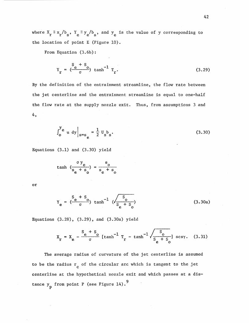
42
Y = (--'=-e ---=--o) h-1 tan T • r o r (3. 29)
By the definition of the entrainment streamline, the flow rate between
the jet centerline and the entrainment streamline is equal to one-half
the flow rate at the supply nozzle exit. Thus, from assumptions 3 and
4,
Jye u I 1 d =- u b 0 y s=s 2 s s"
e
Equations (3.1) and (3.30) yield
cry s tanh (s
e 0 + s ) = s + s e 0 e 0
or
s + s -1 (~ s ( e 0) 0
) y tanh + s e 0 e 0
Equations (3.28), (3.29), and (3.30a) yield
X =X r e
s + s e o
0
-1 [tanh T r
(3.30)
(3.30a)
scsy. (3.31)
The average radius of curvature of the jet centerline is assumed
to be the radius r of the circular arc which is tangent to the jet c
centerline at the hypothetical nozzle exit and which passes at a dis
tance y from point P (see Figure 14). 9 p

Circular Arc Tangent to
43
Jet Centerline at Point A
Figure 14. Geometry of Jet Centerline Curvature

That is,
R = c
R es
44
cl- y )(2R + l- y) + l [ 1 + _2::___-"-p-'--e=-=s'---_.:;::_2 --:---"P-]
2 R (cos2e - 1) - l + Y es p 2 p
(3.32)
where R = r /b ; R = r /b ; Y = y /b . The distance Y can be obtained c c s es es s p p s p
by the definition of the entrainment streamline (refer to Equation
(3.30a)), i.e.,
s + s Y = ( P 0 ) tanh-l
p c:r
,...._
s 0
+ s ) 0
(3.33)
where S = s /b · s = A1P (Figure 14). Referring to Figures 11 and 14, p p s' P
the radius r of the circular arc which is tangent to the entrainment es
streamline at point A1 can be expressed as
r es = [ ds/de ]
1 + dz;/de e=o (3.34)
Equations (3.2), (3.25), (3.34), and z; = tan-l (r::), when combined and
normalized, yield
From Figure 14, the following relations can also be written:
D - l B - (R + l2) sin° 1 2 C es ~
- [ s ] nl = tan ~----------------~-----
s = 2 R e p es p
(R + l) cosf3 + n3 es 2
D - 12 Be - Rc sinS -1 [ s ] n2 = tan ------------~---
Rc cosf3 + n3
(3.34a)
(3.35)
(3.36)
(3. 37)
(3.38)

45
s = R (S + n2) s c (3.39)
where
3.1. 6
D ::d /b s' n3 = d/bs. s s
Numerical Com:eutation Procedure
Given the geometry and control flow rate Q , any steady-state c
value of a variable (e.g., steady-state jet reattachment distance, jet
deflection angle, etc.) can be obtained by numerically solving the basic
equations and the geometric relations derived above. The following are
the list of the basic equations and the geometric relations to be
solved: Equations (3.2a), (3. 7), (3.10), (3.13a), (3.14a) or (3.14b),
(3.15), (3.16a), (3.18) through (3.24), (3.26a), (3.27a), (3.31) through
(3.33), (3.34a), and (3.35) through (3.39). The detailed computation
procedure and computer program listing is given in Appendix C.
The analytical predictions of the steady-state jet reattachment
distance and the jet deflection angle are compared with experimental
data in Chapter V.
3.2 Dynamic Model
For convenience, the transient switching process is divided into
two phases: the process before the jet reattaches to the opposite wall
is called phase I, and the process after the jet reattaches to the oppo-
site wall is called phase II. The criteria for the end of phase I are
given in assumption 6 in section 3.2.1.
3.2.1 Assumptions
The following assumptions are made for the mathematical formulation
of the dynamic model: 10

46
1. The transient switching process can be treated as quasi-steady.
2. The variation in the supply flow rate caused by changes in the
supply nozzle exit pressure is negligible.
3. When the jet reattaches on the output vent area, a "hypotheti-
cal reattachment point" exists between points K1 and K2 (Figure 15), and
momentum is still conserved in the vicinity of the "hypothetical re-
attachment point" (see assumption 5 in section 3.1.1).
4. The edge of the jet is assumed to be the locus of points at
which the jet axial velocity component is 0.1 of the local centerline
velocity. The calculation of the flow passage width a (Figure 17) and v
the flow passage width a (Figure 19) between the jet edge and the oppow
site wall is based on this assumption.
5. The dynamic pressures at the inlet of the OR and NOR output
channels are one-half of the average momentum flux impinging on the in-
let area of the OR and NOR output channels, respectively (see Equations
(3.58) and (3.59) in section 3.2.3.6) [23].
6. Phase I ends when the following conditions are met: (a) the
jet centerline passes the splitter point such that ys ~ d2 - d1 - d3
(see Figure 16), and (b) the flow rate at the exit plane of the OR out-
put channel reaches 95 percent of the steady-state value corresponding
to the total pressure at the inlet of the OR output channel at y = s
d2 - d1 - d3 (see Equation (3.64) in section 3.2.3.7), 11
7. The transition between the end of phase I and the beginning of
phase II is instantaneous. That is, the jet switches over and reattaches
to the opposite wall instantaneously when the conditions given in assump-
tion 6 are met. During the transition, the hypothetical nozzle center
shifts from the intersection of centerlines of supply and control nozzles
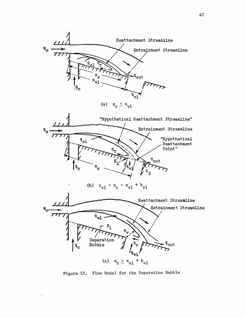
(a)
Reattachment Streamline
X < X r - vl
Entra nment Streamline
"Hypothetical Reattachment Streamline"
(c) x >x 1 +b 1 r- v v
"Hypothetical Reattachment Point"
Figure 15. Flow Model for the Separation Bubble
47
A 0
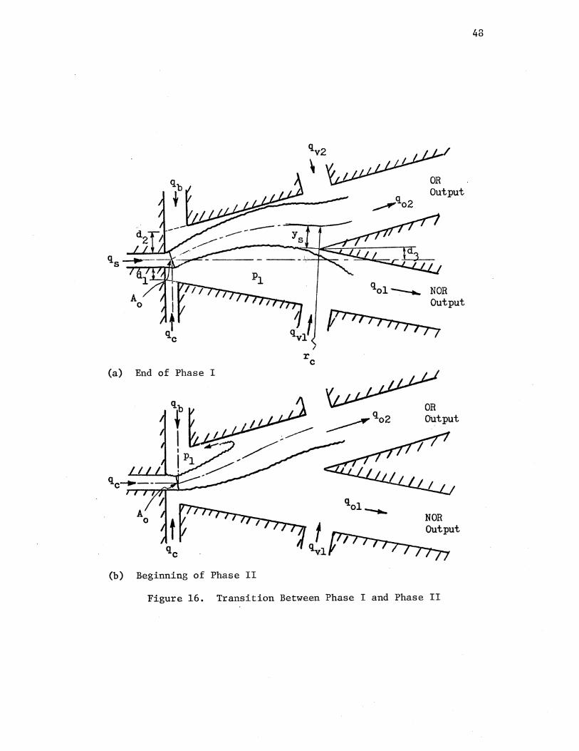
(a) End of Phase I
(b) Beginning of Phase II
/
OR Output
qol--.._ NOR Output
~/~ r c
OR Output
NOR Output
Figure 16. Transition Between Phase I and Phase II
48

(a) F;, > Cl.l
(b) F;, = Cl. 1
I
Figure 17. Output Vent Flow Passage Width
Jet Centerline
49

50
to the intersection of centerlines of supply and bias vent nozzles.
Initial conditions for phase II are those which are associated with the
steady-state reattachment of the jet on the opposite wall for p which tc
exists at the end of phase I.
Remark: Assumptions 6 and 7 are made for the switching process from the
NOR to OR output. Assumptions similar to those are also made for the
switching process from the OR to NOR output (i.e., for the return pro-
cess).
3.2.2 Discussion of Assumptions in Section 3.2.1
This section contains a discussion of the selected assumptions made
in the preceding section:
Assumption 1. The following specific assumptions directly result
from the quasi-steady assumption:
(1) The time rate of change of momentum within control volume 2
(Figure 10) is assumed to be negligible.
(2) Equation (3.16) in section 3.1.4 is assumed to hold, but it
is continuously up-dated at each time step in the dynamic
simulation.
(3) Assumptions 1 through 13, which are made for the steady-state
jet reattachment model in section 3.1.1, are also valid at
each time step in the dynamic simulation.
For the quasi-steady assumption to be valid, the downstream tarvel vela-
city of the jet reattachment point along the wall should be very slow
compared to the jet velocity. In other words, the switching time should
be much larger than the fluid particle transport time through the ampli-
fier, i.e.,
51
d s << t
u s s
where d is the splitter distance downstream of the supply nozzle exit, s
U is the continuity averaged velocity at the supply nozzle exit, and s
t is the switching time [19, 22, 26]. In normalized form, this condis
tion becomes
D << L s s
where D = d /b · T :: U t /b s s s' s s s s This quasi-steady assumption can be justi-
fied only ~ posteriori. Analytical predictions and experimental results
indicate that the normalized switching time is much larger than D ; for s
the geometry chosen in this study, 1" is at least of the order of 20 s
times D (see Figure 34 in Chapter V). s
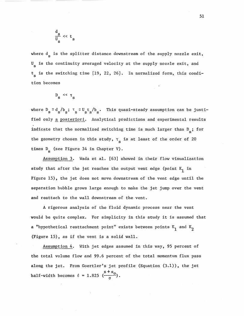
Assumption 3. Wada et al. [63] showed in their flow visualization
study that after the jet reaches the output vent edge (point K1 in
Figure 15), the jet does not move downstream of the vent edge until the
separation bubble grows large enough to make the jet jump over the vent
and reattach to the wall downstream of the vent.
A rigorous analysis of the fluid dynamic process near the vent
would be quite complex. For simplicity in this study it is assumed that
a "hypothetical reattachment point" exists between points K1 and K2
(Figure 15), as if the vent is a solid wall.
Assumption 4. With jet edges assumed in this way, 95 percent of
the total volume flow and 99.6 percent of the total momentum flux pass
along the jet. From Goertler's jet profile (Equation (3.1)), the jet s +s0
half-width becomes o = 1.825 ( ). 0
52
Assumption 6. Assumption 6(a) is based on the experimental study
of the static switching characteristics [63] which showed that the
larger the opposite wall offset, the more the jet is required to pass
the splitter point before the jet reattaches to the opposite wall.
Assumption 6(b) is based on the effect of the fluid inertia in the out
put channel. It was found during the preliminary stage of this study
that for a relatively high control pressure, the analytically predicted
output flow rate was still negative (note the sign convention of the
output flow given in Figure 12) when ys = d2 - d1 - d3 . In other words,
because of the fluid inertia in the OR output channel, the flow which
was initially induced into the internal region of the amplifier was not
completely reversed, even though the jet centerline passed the splitter
point such that ys = d2 - d1 - d3 • It is assumed that the flow in the
OR output channel must be completely reversed and reach the specified
level before the jet reattaches to the opposite wall.
Assumption 7. This assumption is not strictly correct. However,
it is believed that it takes a small time compared to the switching time
for the jet to move from its position at the end of phase I to the posi
tion at the beginning of phase II.
Assumptions 3 through 7, like assumption 1, can be justified only
~ posteriori. The analytically predicted switching times are in good
agreement with experimental data for various offset d1 's and d2 's. Al
though the good agreement does not justify these assumptions on an indi
vidual basis, it suggests justification on a collective basis.

53
3.2.3 Analysis of Phase I
3.2.3.1 Continuity Equation. Referring to Figure 15, the growth
rate of the separation bubble is:
where
for x < x r- vl
for x > x r vl
(3.40)
The flow from the output vent into the separation bubble is re-
stricted by an orifice between the vent edge and the jet edge (i.e., a v
in Figure 15(c)). Assuming the discharge coefficient of the orifice is
unity and the ambient pressure is zero,
(3.41)
Equations (3.5a), (3.6a), (3.40), and (3.41), when normalized, yield
where
2 = u t/b . v - v/b • T s' s s'
A - a /b · X :: X /b • v v s' r r s'
1 2 pl - P/2P Us·
Qc -
xvl
9c19s;
- X /b ; v s
for X < X 1 r- v
(3.42)
54
From Figure 16(a),
where
s
A = R v c
-1 t - tan
s v -- = v - b
s
0 ~
v -- = - b v s
~ - (X cosa - R sinS - l B ) csct v vl 1 c 2 c
R (S + 0 c
s 1.825 ( v
+ s a
0)
1 -- B
2 c ]
(3. 43)
If the reattachment point moves far downstream of the output vent, the
separation bubble becomes completely open to the vent and the flow
through the vent is restricted only by the vent width bvl· In the ana-
lytical model, this case is represented as follows: the term A in v
Equation (3.42) is replaced by Bvl = bv1/bs if t ~ a1 (see Figure 16b).
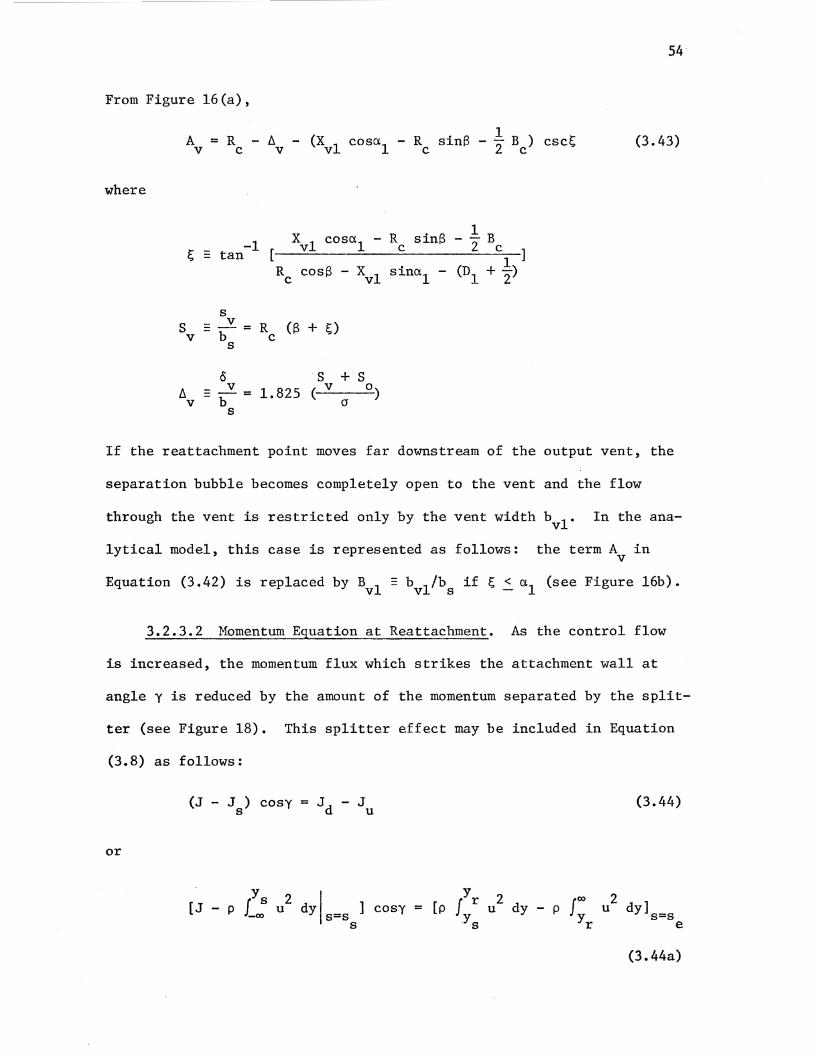
3.2.3.2 Momentum Equation at Reattachment. As the control flow
is increased, the momentum flux which strikes the attachment wall at
angle y is reduced by the amount of the momentum separated by the split-
ter (see Figure 18). This splitter effect may be included in Equation
(3.8) as follows:
(3.44)
or
. Ys 2 I [J - p Lt) u dy s=s ] cosy
s Jyr 2 Joo 2 d ]
= [p y u dy - p u y s=s s ~ e
(3.44a)

Reattachment Streamline
Entrainment Streamline
J Jet Centerline
Attachment r '~-'\' 1\s / ~ Jd Wall ~--~~--L---~
Splitter
Control Volume 2
Figure 18. Momentum Balance in the Vicinity of the Reattachment Point
Ln Ln

Equations (3.1) and (3.44a), when combined and normalized, yield
(1 - l T + l T3) cosy = -1 + 3T 2 s 2 s r
where
crY T tanh Cs
s ) ; T - + s -s r s 0
y = y /b . y - y /b . s s s s' r r s' s
Solving Equation (3.45) for T , we get r
where
T r
-1 2cos [~+cos (A/2)]
3
tanh
- s s
crY
Cs r )
+ s e 0
/b . s
' (1 - l T + l T3) + 1 + l T - l T3 A = 2 s 2 s cosy 2 s 2 s·
56
(3.45)
(3.46)
This treatment of the splitter effect is similar to that employed by
Goto and Drzewiecki [23].
3.2.2.3 Unattached-Side and Separation Bubble Pressures. As the
jet moves toward the opposite wall, the spacing a between the opposite w
wall and the jet edge restricts the flow from region 2b into region 2a
(see Figure 19). Thus, the average pressure in region 2a becomes less
than the average pressure in region 2b. This nonuniform pressure dis-
tribution in the unattached-side is confirmed by the results of static
pressure measurements along the opposite wall [36].
It is assumed that the unattached-side pressure is represented by
two pressures: average pressure p2a in region 2a and average pressure
p2b in region 2b. At each time step, the normalized pressure P2a is
PLEASE NOTE:
Dissertation contains small and indistinct print. Filmed as received.
UNIVERSITY MICROFILMS.

~ r ):,b
\1v~
~0
Figure 19. Flow and Geometric Model for UnattachedSide Pressure
57
Region 2b
____., ~02.
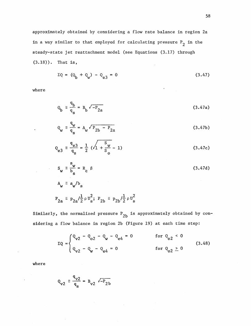
58
approximately obtained by considering a flow rate balance in region 2a
in a way similar to that employed for calculating pressure P2 in the
steady-state jet reattachment model (see Equations (3.17) through
(3.18)). That is,
EQ = (Qb + ~) - Qe3 = 0
where
Qb - qb
Bb /-P2a - = qs
-~ ~ = -= Aw /p2b - p
qs 2a
Q - qe3 - l ch + sw - 1) e3 - qs - 2 S 0
A w
- a /b w s
(3 .47)
(3.47a)
(3.47b)
(3.47c)
(3.47d)
Similarly, the normalized pressure P2b is approximately obtained by con
sidering a flow balance in region 2b (Figure 19) at each time step:
where
qv2 = -- =
Q = 0 e4 for Q < 0 o2
(3.48)

59
_ qe4 1 /S Q = - = - (11 + ~ - 1) - Q e4 q 2 S e3
s 0
and Q02 is given by Equation (3.56a) in section 3.2.3.6. In the second
equation of Equation (3.48), it is assumed that all flow into the OR
output channel comes from the jet if Q02 > 0. Since Equations (3.47)
and (3.48) cannot be solved explicitly, a suitable iteration method has
to be used to determine P2a and P2b (see Appendix C for detail).
12 as
where
From Figure 19, the normalized flow passage width A can be written w
A w
1 1 = (R sin8 + - B ) tana2 + n2 + - - R (1 - cos8) c 2 c 2 c
0 s + s !'J.w = bw = 1.825 ( w a o)
s
!1 w
(3.49)
The separation bubble pressure may be obtained by substituting the
average unattached-side pressure P2 into Equation (3.16a), i.e.,
where
2 R
c (3.50)
3.2.3.4 Jet Deflection. The jet deflection angle can be obtained
by substituting the pressure P2a for P2 in Equation (3.13a), i.e.,
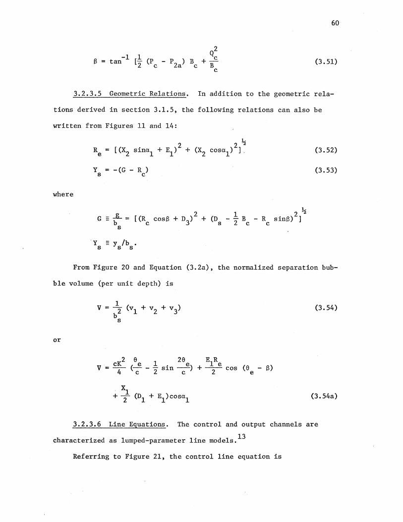
60
-1 1 8 = tan [- (P - P ) B 2 c 2a c (3. 51)
3.2.3.5 Geometric Relations. In addition to the geometric rela-
tions derived in section 3.1.5, the following relations can also be
written from Figures 11 and 14:
(3.52)
Y = -(G - R ) s c (3.53)
where
. y - y /b . s s s
From Figure 20 and Equation (3.2a), the normalized separation bub-
ble volume (per unit depth) is
1 V = b2 (vl + v2 + v3) (3.54)
s
or
(3.54a)
3.2.3.6 Line Equations. The control and output channels are
characterized as lumped-parameter line models. 13
Referring to Figure 21, the control line equation is

Jet Centerline
Entrainment Streamline
el
Figure 20. Cross Section of Separation Bubble
0'\ I-'
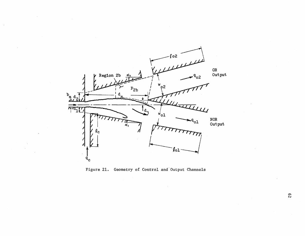
r---'02 --j ___.,..qo2
----.....qol
Figure 21. Geometry of Control and'Output Channels
OR Output
NOR Output
0'1 N
2 I dq + _C _ _£
cdc dt
63
(3.55)
where I ~ pt /b , and p is the total pressure at the inlet of the c c c tc
control channel. Friction losses and contraction effects in the control
channel are accounted for through use of the discharge coefficient Cdc
(Cdc~ (qc) actual I (qc) ideal) [23]. Further discussion of the dis-
charge coefficient is given in Appendix B.
In normalized form, Equation (3.55) becomes
2 dQ c p
tc + dT
where
p tc
I' ~ 21 /B · c c c'
and P is given by Equation (3.14a). c
(3.55a)
Similarly from Figure 21, the following output line equations may
be written for the OR and NOR output channels, respectively:
where
P2b + Pd2
P2b + Pdl
I o2
1 -p 2
1 = 2 p
qo2,qo21 dq 2
2 + I __ o_ o2 dt
wo2
qol,qoll dq 1 + I __ o_
2 ol dt wol
(3.56)
(3.57)
and pd2 and pdl are the dynamic pressures at the inlet of the OR and
NOR output channels, respectively.

64
The total pressures (p2b + pd2) and (p2b + pdl) are considered as the
internal "driving force" to the OR and NOR output channels, respec-
. 1 14 t1ve y. Friction losses in both output channels are assumed negligi-
ble. Equations (3.56) and (3.57), when normalized, yield
p2b + pd2 Qo21Qo21
+ I' dQo2
= w2 o2 dT
o2
(3.56a)
QoliQoll dQ p2b + pdl = + I I ____Q_!_
w2 ol dT ol
(3.57a)
where
1 2 1 2 pd2 - Pdz'2 pUs; pdl - Pd/2 pUs;
I' o2 - 2Lo2/'~vo2; I' ol - 2Lol/Wol;
Lo2 - t zlb ; Lol - t 1/b ; 0 s 0 s
wo2 = w 2/b ; wol - w /b • 0 s 0 s
Referring to Figures 18 and 21 and assumption, 5, the dynamic pres-
sures at the inlet of the OR and NOR output channels are:
Js p ,Ys 2 I p d2 = ~ = ~ LX> u dy s=s
o2 o2 s (3.58)
= _l = _P_ Jyr 2 d I 2w 1 2w 1 y u Y s=s
o o s e (3.59)
Equations (3.1) and (3.58) and Equations (3.1) and (3.59), when combined
and normalized, yield respectively:
pd2 1 (2 + 3T - T3) =--
4Wo2 s s (3.58a)
pdl 1 (3T - T3 - 3T + T3) =--
4Wol r r s s (3.59a)
65
Output channel widths are provided from the geometry or can be ob-
tained from other geometric parameters, i.e. (from Figure 21),
(D2 1 + D sina2 (3.60) wo2 = D3 + 2) cosa2 s
wol (Dl 1 sina1 • (3.61) = + D3 + Z) COSCI.l + D s
3.2.3.7 End of Phase I. By assumption 6, phas~ I ends when the
following conditions are met:
and
where
y > y s- I
-y I
3.2.4 Analysis of Phase II
(3.62)
(3. 63)
The basic equations and geometric relations for phase II are
briefly presented without detailed derivations because of their similar-
ity in form to those for phase I.
3.2.4.1 Continuity Equation. Referring to Figure 22 and Equation
(3.42), the growth rate of the separation bubble is (in normalized
form):
+.l h s Qb (1 - T +~)
2 r s for~ 2 ~2 dV 0
-= dT
h s Qb +.l (1 - T + S e)+ Av ~
2 r .L for ~ > ~2
0
(3.64)
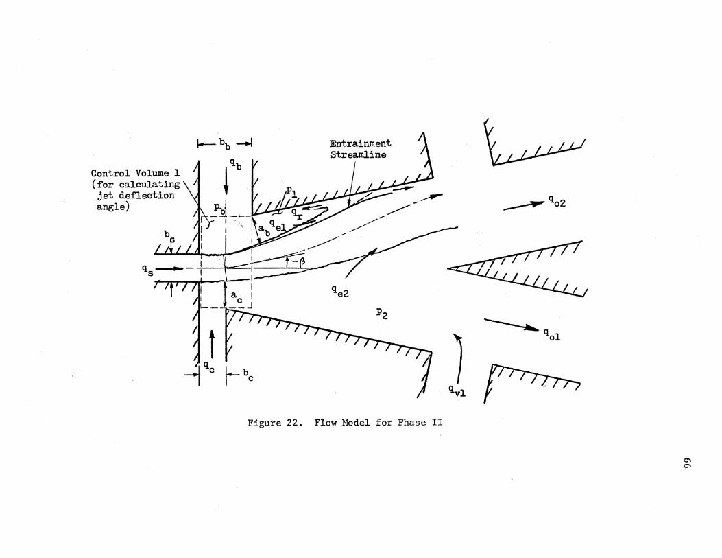
Control Volume 1 (for calculating jet deflection angle)
~bb --1
q ---- I Y ...........--, I I --S =
;, t --1 qc j- be
p2
Figure 22. Flow Model for Phase II
J qvl
___.,..qo2
------.... qol
0\ 0\
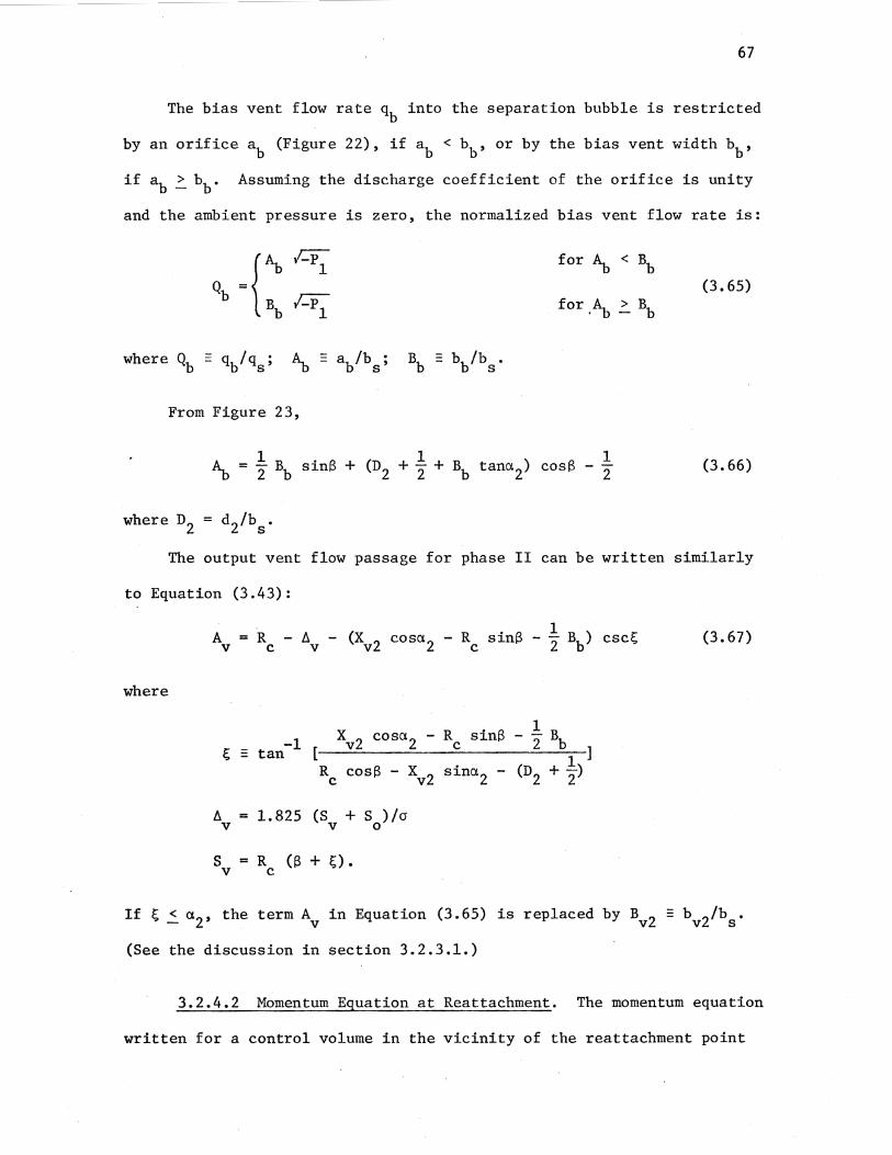
67
The bias vent flow rate qb into the separation bubble is restricted
by an orifice ab (Figure 22), if ab < bb, or by the bias vent width bb'
if ab ~ bb. Assuming the discharge coefficient of the orifice is unity
and the ambient pressure is zero, the normalized bias vent flow rate is:
(3.65)
From Figure 23,
1 --2
(3.66)
The output vent flow passage for phase II can be written similarly
to Equation (3.43):
where
A v
~
!J. v
s v
-
=
=
tan -1 [ xv2 cosa2 -
R cosS - xv2 c
1.825 (S + S )/cr v 0
R (S + 0. c
R sinS 1 --B
c 2 b ] 1 sina2 - (D2 + z)
If ~ 2 a2 , the term Av in Equation (3.65) is replaced by Bv2
(See the discussion in section 3.2.3.1.)
(3. 67)
- b 2/b • v s
3.2.4.2 Momentum Equation at Reattachment. The momentum equation
written for a control volume in the vicinity of the reattachment point
68
I bp•
I
-p
I
Figure 23. Bias Vent Flow Passage Width

69
is identical in form to that for phase I (Equation (3.46)). That is,
-1 [7f + (A./2)] T 2cos cos (3.46) r 3
where
A. 3 + .!_ T3) 1 + l T - .!_ T3 = (1 -- T cosy + 2 s 2 s 2 s 2 s
T - tanh [crY /(S + S )]. s s s 0
3.2.4.3 Unattached-Side and Separation ·Bubble Pressures. If the
jet deflection angle is negative (note that the sign convention of S is
c.hanged in phase II; see Figure 22), the minimum area between the jet
edge and the attachment wall is the flow passage width a (see Figure c
22). Thus, it is assumed that the unattached-side pressure is repre-
sented by the single average pressure p2 in the region downstream of ac.
At each time step, the normalized pressure P2 is approximately obtained
by considering a flow rate balance in the region downstream of a in a c
way similar to that employed for calculating pressure P2 in the steady
state jet reattachment model (see Equations (3.17) through (3.18)).
That is,
where
Qvl Bvl ;-::p:
2
Qe2 qe2 1 (;{ + ss - 1) - --=-qs 2 s
0
and S is similarly defined as that shown in Figure 19. s
(3.68)
70
If the jet deflection angle becomes positive with decreased con-
trol flow, the unattached-side pressure is assumed to be represented by
two pressures: average pressure p2. in region 1 and average pressure a
p2b in region 2, which are similarly defined as those for phase I (see
Figure 19). Referring to Equation (3.47), the normalized pressure P2a
at each time step is approximately determined by
EQ = (Q + 0 ) - Q = 0 c 'w e3
where
~ = A /p2b - p w 2a
1 (;;_ s Qe3 =- +_3!...- 1)
2 s 0
s = R 8 w c
A - a /b w w s
1 2 p2a - P2a12 Pus
p2b = 1 2
P2b12 Pus
and a is similarly defined as that shown in Figure 19. w
(3.69)
Referring to Equation (3.48), the normalized pressure P2b at each
time step is approximately determined by
where
for Q < 0 ol
for Q01 > 0 (3. 70)

71
and Q01 is given by Equation (3.58) in section 3.2.3.6. Iteration pro
cedures for solutions to Equations (3.68) through (3.70) are given in
Appendix C.
where
The area A can be written similarly to Equation (3.49): w
s + s ~ = 1.825 ( w 0).
w CJ
(3. 71)
Referring to Figure 22 and Equation (3.50), the separation bubble
pressure is:
p2 2
for S < 0 R c
pl = (3.72) s s (~) w 2
p2a + p2b (1- -) R for S > 0. s s s s c
3.2.4.4 Jet Deflection. As shown in Figure 22, the supply jet
interacts with the control and bias vent flows in control volume 1 dur-
ing phase II. It is assumed that the bias vent flow has a momentum
interaction with the supply jet in the control volume during phase II.
The return flow in the separation bubble has a tendency to make the vent
flow impinge directly on the supply jet. Referring to Figure 22 and
Equation (3.51),
(3.73)
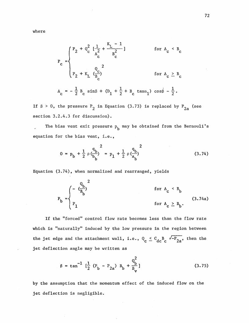
where
p = c
p2 + Q~ for A < B c c
for A > B c- c
72
If 8 > 0, the pressure P2 in Equation (3.73) is replaced by P2a (see
section 3.2.4.3 for discussion).
The bias vent exit pressure pb may be obtained from the Bernouli's
equation for the bias vent, i.e.,
2 1 qb
= pl +- p(-) 2 ab
Equation (3.74), when normalized and rearranged, yields
r (Qb)
2
for A < Bb Bb c
pb pl for A > Bb. c-
(3.74)
(3.74a)
If the "forced" control flow rate becomes less than the flow rate
which is "naturally" induced by the low pressure in the region between
the jet edge and the attachment wall, i.e., Q < Cd B ~2 , then the c- c c a
jet deflection angle may be written as
(3.75)
by the assumption that the momentum effect of the induced flow on the
jet deflection is negligible.
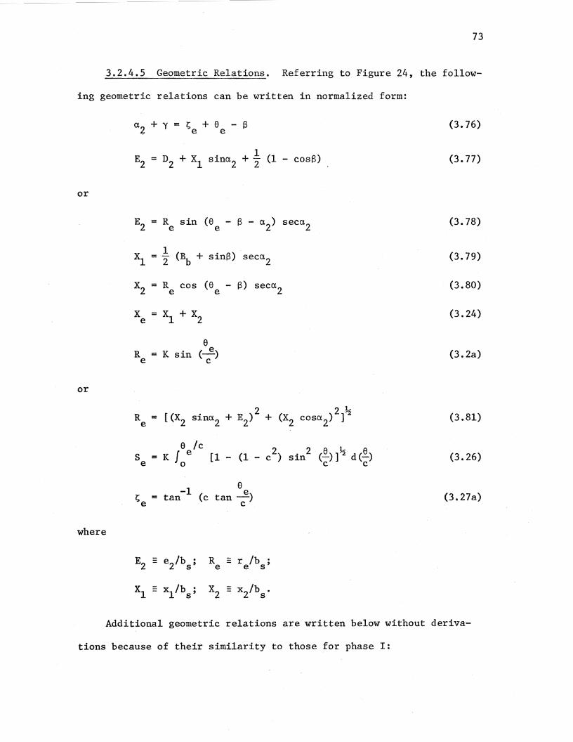
73
3.2.4.5 Geometric Relations. Referring to Figure 24, the follow-
ing geometric relations can be written in normalized form:
or
or
where
X = e
= r; + e - s e e
R cos (8 - S) seca2 e e
e R = K sin (~)
e c
-1 e I; = tan (c tan ~)
e c
E2 - ezlbs; R - r /b · e e s'
xl - x/bs; x2 - xz!bs.
(3.76)
(3. 77)
(3.78)
(3.79)
(3.80)
(3.24)
(3.2a)
(3.81)
(3.26)
(3.27a)
Additional geometric relations are written below without deriva-
tions because of their similarity to those for phase I:
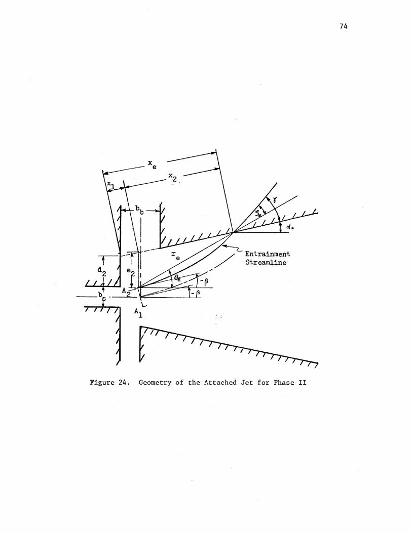
74
~ / Entrainment
/ Streamline /
Figure 24. Geometry of the Attached Jet for Phase II

where
and
where
and
where
cl- y >C2R + l- Y > 1 2 p es 2 p R = R + - [1 + ---'"""-------:--..... -
c es 2 R (cos28 - 1) - l + Y es p 2 p
R . = K/2c es
s = 2R e p es p
1 e = - (S + n ) p 2 1
_1 [Ds - ~ Bb - (Res + ~) sinS n = tan --'------------]
1 (Res + ~) cosS - D3
S = R (S + n2 ) s c
-1 n = tan 2
D - l B - R sinS [ s 2 b c ]
1 (2 + Rc) cosS - n3
Y = -(G - R ) s c
75
(3.41)
(3.82)
(3. 83)
(3.84)

76
G = [ (R c
2 1 2 k cosS- D) + (D -- B - R sinS) ) 2
3 s 2 b c
and
CK2 8 l 28 E2R V ( e . e ) + e (8 o) = 4 c - 2 sJ.n -c- --2- cos e - IJ
(3.85)
3.2.4.6 Line Equations. The control line equation (Equation
(3.55a)) and the output line equations (Equations (3.56a) and (3.57a))
are used both for phase I and for phase II. But, the equations for the
dynamic pressures Pdl and Pd2 should be modified as follows because of
the jet reattachment to the opposite wall during phase II:
pd2 1 (3T - T3 - 3T + T3) =--
4Wo2 r r s s (3.86)
pdl 1 (2 + 3T - T3) =--
4Wol s s (3. 87)
3.2.4.7 End of Phase II. It is assumed that the jet switches
back and reattaches to the attachment wall when the following conditions
are met:
and
y > 0 s-
3.2.5 Digital Simulation
(3.88)
(3.89)
The analytical dynamic model formulated above may be simulated on
a digital computer (IBM 370/158) using DYSI~~ (Dynamic Simulation
77
15 Program). The following are the list of the basic equations and the
geometric relations to be simulated on the computer: Equations (3.2a),
(3.19) through (3.24), (3.26a), (3.27a), (3.31) through (3.33), (3.34a),
(3.35) through (3.39), (3.42), (3.43), (3.46) through (3.53), (3.54a),
(3.55a), (3.56a), (3.57a), (3.58a), (3.59a), (3.60) through (3.73),
(3.74a), and (3.75) through (3.89). A computer flow chart and computer
program listings are given in Appendix C.
The analytical predictions of the switching time, the return time,
and the transient response are compared with experimental data in
Chapter V.
ENDNOTES
1Hoynihan and Reilly [40] showed in their experimental study on the jet deflection in a proportional fluid amplifier that the effective "pivot point" of the deflected jet is approximately at the intersection of the centerlines of the supply and control nozzles.
2The entrainment streamline is defined as the line which originates at point A1 (Figure 10) and divides the flow originally in the jet from the fluid entrained by the concave side of the jet.
3 Errors due to this assumption are of the order of 10 percent of
sf for Q = 0 and 1 percent of sf for Qc = 0.3 for a typical geometry of a monost£ble fluid amplifier.
4This assumption is not strictly correct. Sawyer [57] indicated that the rate of fluid entrainment is greater on the convex side of the jet than that on the concave side of the jet. However, Epstein [19] showed that the analytically predicted jet reattachment distances obtained from Sawyer's model [57] (Sawyer used the different rate of entrainment on each side of the jet) are almost identical to those obtained from Bourque's model [6] (Bourque used the same rate of entrainment on both sides of the jet). Both Bourque and Sawyer treated only the jet reattachment problem with no control flow.
5This assumption is based on the flow visualization and velocity profile measurements of the interacting jets by Douglas and Neve [14].
6Epstein [19] assumed (1) that the control and supply jets form a combined jet emerging from a "hypothetical nozzle" after the momentum interaction; (2) the reattachment streamline as the separation bubble boundary, while in the present model the entrainment streamline is assumed as the boundary to be consistent with assumption 2. In the present steady-state model, the reattachment streamline is defined as the line which originates at point I (Figure 10) and divides the flow proceeding downstream along the wall from the flow recirculating within the separation bubble; and (3) the control nozzle exit pressure p (Figure 10) is known for the calculation of the jet deflection an~le, but in the present model p is determined analytically (see section 3.1.4 for detail). c
78
79
7Referring to assumptions 2, 3 and 4, the value of s can be determined by matching the flow rate through the hypothetical Razzle to the flow rate determined by integrating Goertler's velocity profile at distances from the "virtual origin" of the jet, i.e.,
0
Using Equation (3.1), the above equation reduces to s 0
8Epstein [19] demonstrated that the error introduced by this approximation is less than 0. 5 percent of the exact value for 0 < e I c < 4/9 1T and near 1.5 percent for 4/9 1T < e /c < TI/2. e
e
9 The error incurred by taking Yp from point P instead of from the entrainment streamline is less than 0.3 percent of Rc for D1 = 0.5, Ds = 11, a1 = 12°.
10 These assumptions are discussed in section 3.2.2.
11 For a bistable fluid amplifier, Goto and Drzewiecki [23] assumed that phase I ends when y = 0.
s
12A • d h . . b h . d d h ~~ 1s assume t e m1n1mum area etween t e Jet e ge an t e oppo-site wall. It is believed that this assumption is adequate for the determination of approximate values of P2a and P2b.
13rhis lumped-parameter approximation is valid whenever the time required for a pressure signal to travel the length of the line is short with respect to the period of the highest frequency signal that is to be transmitted. For the test amplifier used in this study, the period of the highest frequency pressure signal in the control line is of the order of 1 millisecond, while the time required for the signal to travel 1 inch long control channel is of the order of 0.1 millisecond
( 1 in. = 10-4 sec). 1000 x 12 in/sec
14This "driving force" concept is attributed to Goto and Drzewiecki [23].
15DYSIMP is a packaged program for the digital simulation of dynamic systems, which is written in FORTRAN IV. It has been developed by the School of Mechanical and Aerospace Engineering, Oklahoma State University.
CHAPTER IV
EXPERIMENTAL APPARATUS AND PROCEDURE
4.1 Apparatus
Experimental work was carried out on a large-scale test model (about
ten times actual size) of a typical monostable fluid amplifier. Figure
2~ is a plan view and Figure 26 is a photograph of the test amplifier.
The major components of the test amplifier were a base plate, a cover
plate, and movable internal blocks. By using a large-scale amplifier
rather than an actual sized one, it was possible (1) to locate the in-
ternal blocks accurateJy, and (2) to lengthen the switching and return
times, thereby enhancing accuracy of measurement of these quantities.
The interior geometry of the amplifier was formed with seven 0.31
inch thick aluminum blocks. Except for the two nozzle blocks, slots
were provided for each block to allow a certain range of adjustment (see
arrows in Figure 25). Gage blocks (Fonda Gage Company) and a vernier
caliper were used to locate these blocks. After these blocks were firm-
ly bolted to a 1/2 inch thick aluminum base plate, a 1/2 inch thick
plexiglass cover plate was attached to the top of the device and then the
entire assembly was fastened by 24 setscrews. Silicon lubricant was
applied between the plates to minimize leakage.
The supply nozzle width (b ) was fixed at 0.1 inch, which resulted s
in an aspect ratio of 3.1. Wire screens and sponge-type packing material
80
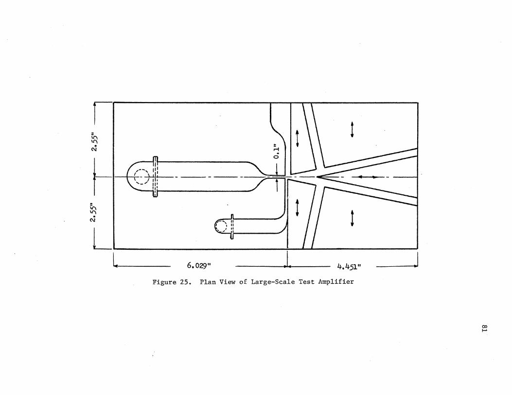
I i:r'l 1.1"'\ . C\l
f-~ 1.1"'\ . C\l
L
1
1
L 6. 029" j_
4.451"
Figure 25. Plan View of Large-Scale Test Amplifier
_I
00 1-'

82
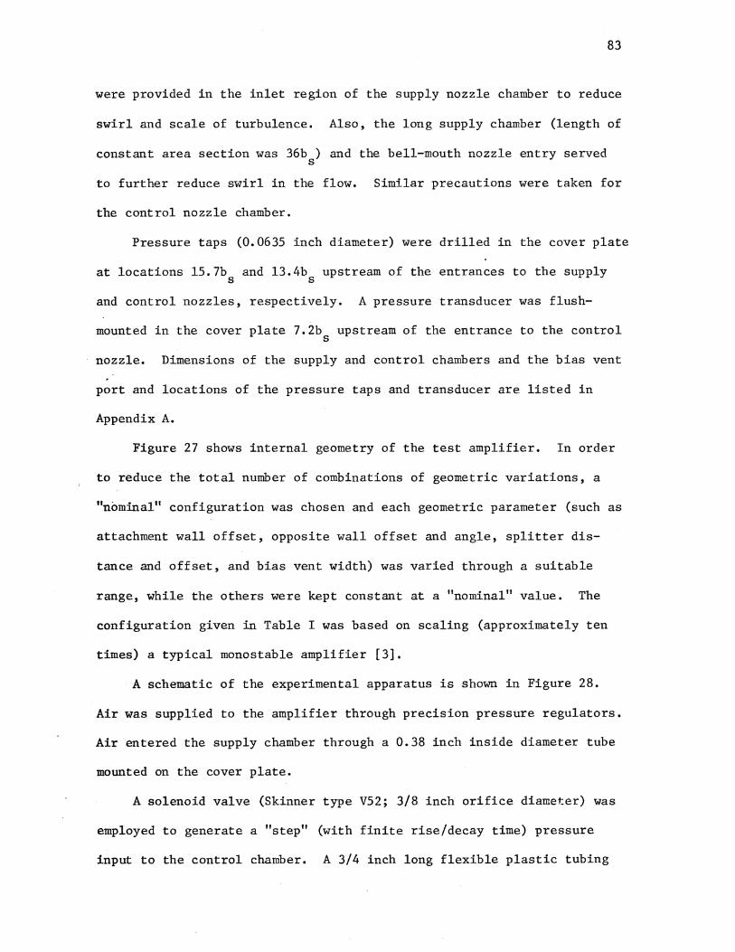
83
were provided in the inlet region of the supply nozzle chamber to reduce
swirl and scale of turbulence. Also, the long supply chamber (length of
constant area section was 36b ) and the bell-mouth nozzle entry served s
to further reduce swirl in the flow. Similar precautions were taken for
the control nozzle chamber.
Pressure taps (0.0635 inch diameter) were drilled in the cover plate
at locations 15. 7b and 13.4b upstream of the entrances to the supply s s
and control nozzles, respectively. A pressure transducer was flush-
mounted in the cover plate 7.2b upstream of the entrance to the control s
nozzle. Dimensions of the supply and control chambers and the bias vent
port and locations of the pressure taps and transducer are listed in
Appendix A.
Figure 27 shows internal geometry of the test amplifier. In order
to reduce the total number of combinations of geometric variations, a
"nominal" configuration was chosen and each geometric parameter (such as
attachment wall offset, opposite wall offset and angle, splitter dis-
tance and offset, and bias vent width) was varied through a suitable
range, while the others were kept constant at a "nominal" value. The
configuration given in Table I was based on scaling (approximately ten
times) a typical monostable amplifier [3].
A schematic of the experimental apparatus is shown in Figure 28.
Air was supplied to the amplifier through precision pressure regulators.
Air entered the supply chamber through a 0.38 inch inside diameter tube
mounted on the cover plate.
A solenoid valve (Skinner type V52; 3/8 inch orifice diameter) was
employed to generate a "step" (with finite rise/decay time) pressure
input to the control chamber. A 3/4 inch long flexible plastic tubing

1o2
lt:~L~" ds bs T ~~ , -L,-,1 ••
--.J
d?_fk,- ,-. 1 ---~..J..-f.,._.
lol
Figure 27. Internal Geometry of the Test Amplifier
co ~

TABLE I
NOMINAL CONFIGURATION
Geometric Parameter
Supply nozzle width (b ) s
Control nozzle width (b /b ) c s
Bias vent width (bb/bs)
Attachment wall offset (d1/bs)
Opposite wall offset (d2/bs)
Attachment wall angle (a1)
Opposite wall angle (a2)
Attachment wall length (x 1/b ) v s
Opposite wall length (x 2/b ) v s
Splitter ~istance (d /b ) s s
Splitter offset (d3/bs)
NOR output vent width (b 1/b ) v s
OR output vent width (b 2/b ) v s
NOR output channel length (~ 1/b ) 0 s
OR output channel length (~ 2/b ) 0 s
Control channel length (~ /b ) c s
Aspect ratio (AR)
85
Nominal Geometry
0.10 inch
1.00
2.00
0.50
1.00
12°
12°
10.94
10.94
11.00
0.00
3.05
3.05
32.34
32.34
9.69
3.10
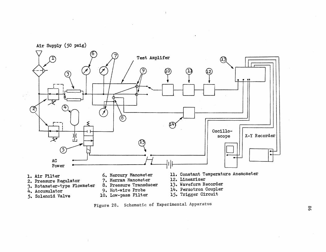
Air Supply (SO psig)
~- CI{ ~ 1 l \ I ...--- _._ -r---L----"'J,__
or---k-__,j_j
lli 0~
AC 1 Power :~
1. Air Filter 2. Pressure Regulator ), Rotameter-type Flowmeter 4. Accumulator 5. Solenoid Valve
~
6. Mercury Manometer 7. Merram Manometer 8. Pressure Transducer 9. Hot-wire Probe
10. Low-pass Filter
e( Oscillo
scope
D
--rl-1-----~-~-~'
X-Y Recorder
11. Constant Temperature Anemometer 12. Linearizer 1). Waveform Recorder 14. Perzotron Coupler 15. Trigger Circuit
Figure 28. Schematic of Experimental Apparatus 00 0\

87
(3/8 inch inside diameter, 1/2 inch outside diameter) was used to connect
the solenoid valve outlet to the control chamber inlet through the base
plate. This flexible line minimized the transmission of vibrations from
the solenoid valve to the pressure transducer in the control chamber.
4.2 Instrumentation and Measurement Procedure
The following quantities were measured:
1. Jet centerline axial velocity distribution in the semi-confined
jet (cover plates, but no side walls or splitter).
2. Switching and return times.
3. NOR output total pressure transient response.
All measurements were conducted with a supply total pressure of 10
in. H20, with one exception. The measurements of the jet centerline
axial velocity distribution were also carried out for a supply total
pressure of 20 in. H20 in order to determine any first order effects due
to Reynolds number. The Reynolds number associated with the supply total
pressures of 10 in. H20 and 20 in. H20 are approximately 1.4 x 10⁴ and
9.8 x 10³, respectively. 1
The supply total pressure was measured with a Meriam manometer con-
taining unity oil, and the supply volumetric flow rate was measured with
two identical Fisher-Porter rotameter-type flowmeters (FP-1/2-G-10/80)
connected in parallel. The static pressure just downstream of the flow-
meters was measured with a mercury manometer.
Jet centerline axial velocities in the semi-confined jet (no side
walls and splitter) were "computed" from the total pressure measurements
along the jet axis, assuming the static pressure was constant throughout
the jet field. The total pressure was measured midway between the top

88
and bottom plates with a standard total pressure probe (0.065 inch out
side diameter) mounted on a traverse mechanism, and a Meriam manometer.
Switching time is defined in this study as the time elapsed from
the instant the control total pressure is observed to rise in the con
trol chamber until the velocity at the exit plane of the OR output
channel reaches 95 percent of the final value. Similarly, return time
is defined as the time elapsed from the instant the control total pres
sure is observed to decay in the control chamber until the velocity at
the exit plane of the NOR output channel reaches 95 percent of its final
value.
A Kistler Piezotron pressure transducer (Model 201B5) with a Piezo
tron coupler (Model 587D) was used to measure the control chamber total
pressure. The transducer was calibrated by measuring the control total
pressure at the steady-state condition with a Meriam manometer.
The output velocity was measured with a DISA hot-wire (Type 55F31)
probe located at the exit plane of the OR (or NOR) output channel. A
DISA hot-wire anemometer system (Type 55A01 constant temperature anemo
meter and Type 55Dl0 linearizer) was employed for this measurement. An
external 7 kc low-pass filter was used to eliminate high frequency jet
noise effects in the velocity signal trace.
The control pressure and output flow rate signals were digitized
and stored by a Biomation Waveform Recorder (Model 1015). The Biomation
Recorder was capable of storing 1024 ten-bit words. The sampling inter
val for the series of measurements was 0.02 to 0.1 millisecond. Once
signals were stored in the Biomation Recorder, they could be retrieved
and displayed on an oscilloscope (Tekronix Model 5103N). The switching
(or return) time was determined directly from the displayed control
89
pressure and output velocity traces as defined above. Typical traces
are shown in Figures 6 and 7.
The output total pressure transient response was measured with a
total pressure probe located at the exit plane of the NOR output chan-
nel. The total pressure probe was connected to a Kistler Piezoelectric
pressure transducer (Model 6011); the transducer was connected to a
Kistler charge amplifier (Model 504A). The transient output pressure
signal was digitized and stored by a Biomation Recorder. This signal
was retrieved and plotted on a Hewlett Packard X-Y recorder (Model
135A). With the plotting speed of the order of 50 seconds, the transi~
ent signal could be reproduced quite precisely without adding undesir-
able dynamics of the plotting instrument.
It was found that as the control total pressure increased, the
supply chamber total pressure also increased due to the increased pres-
sure in the supply nozzle exit region. (That is, there is some coupling
between the supply and control pressures.) However, the supply flow
rate remained almost constant even when the control pressure increased
to 10 in. H20 (the decrease in the supply flow rate was less than 1.5
percent of that with zero control pressure). This effect was also ob-
served by Weikert and Moses [65]. For each set of measurements, the
supply total pressure was set to 10 in. H20 with the control chamber
open to ambient pressure, and the supply flow rate was measured. This
supply flow rate measurement was used to compute the supply jet dynamic 2
1 (qs) pressure 2 p bs

ENDNOTE
1 Based on the supply nozzle width: Re - U b /v. s s s
90
CHAPTER V
RESULTS AND DISCUSSION
Unless otherwise mentioned, the coordinates of the graphs presented
in this chapter are normalized with respect to the associated variables
defined in Chapter III. The following measured values were used for the
normalization:
qs = 230.9 . 2/ 1n sec
u qs
2309 in/sec = -= s b s
1 u2 0.3 psig (8.28 in. H20) 2 s
b 4.33 x 10⁻² millisecond. tt
s = -= u s
5.1 Jet Spread Parameter
Goertler's jet velocity profile [31] given by Equation (3.1) has an
experimentally derived parameter a which is called a jet spread parameter.
A value of a= 7.67 was found for the two-dimensional jet [58]. However,
that value of a does not hold for the semi-confined jet because the top
and bottom plates reduce the jet entrainment. A value of a for the semi-
confined jet can be determined either by measuring the transverse velo-
city profile at a given axial distance from the nozzle, or by measuring
the jet centerline axial velocity distribution.
91

92
Figure 29 shows jet centerline axial velocity distributions in the
semi-confined jet (no side walls and splitter; aspect ratio= 3.1). The
measured velocities are normalized with respect to continuity averaged
velocity U at the supply nozzle exit plane. The uncertainty in these s
uc measurements is of the order of one percent of full scale (Us= 1.0).
Due to the boundary layer development in the nozzle, u /U is greater c s
than one in the "zone of flow establishment." Goertler's theory [31]
with a = 10.5 yields best match with the experimental data for s/b > 25 s
(the length of the entrainment streamline during the switching process
is 3 < s /b < 35 for the monostable fluid amplifier with the nominal e s
geometry). Since the constant-velocity "potential core" region is not
considered in Goertler's theory, the agreement between his theory and the
experimental data is generally poor in the "zone of flow establishment."
For the range of 4 < s/b < 15, a = 20 yields better agreement with the s
experimental data than a = 10.5.
Although it is possible to use Albertson 1 s two-dimensional theory
[31; dashed line in Figure 29] in the dynamic modeling of a monostable
fluid amplifier, the resulting equations will be unnecessarily complex
and difficult to solve. Two previous studies [6, 46]1 provide justifica-
tion for using Geortler's profile in the present study.
5.2 Comparison of Steady-State Jet Reattachment
Model Predictions With Experimental. Data
One of the contributions of the present work to the literature is
the development of the steady-state jet reattachment model which can cor-
rectly predict the steady-state jet reattachment distance and jet deflec-
tion angle.
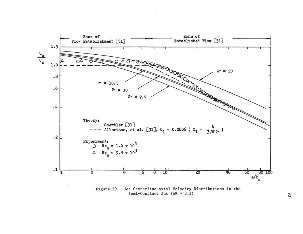
u _c u s
r-- Zone of . ·I Zone of Flow Establishment [31] Established Flow [31]
1.5
1.0
I .8
I
.6 '-
.4
.2
~~ / rr = 20
f1' = 10.5
0'- = 10
0'- = ?.7
Theory: Goertler [31] 4 Albertson, et al. [31], c1 = 0.0806 ( c1 = ":! rwrt.. }
Experiment: 4 0 Re = 1.4 X 10 s 6 Re :: 9.8 X 10³
s
.,
11 I ~ ~ s 1· I 45 I 8 I • 1 2 10 20 6oo 100
Figure 29. Jet Centerline Axial Velocity Distributions in the Semi-Confined Jet (AR = 3.1)
s/b s
\0 w
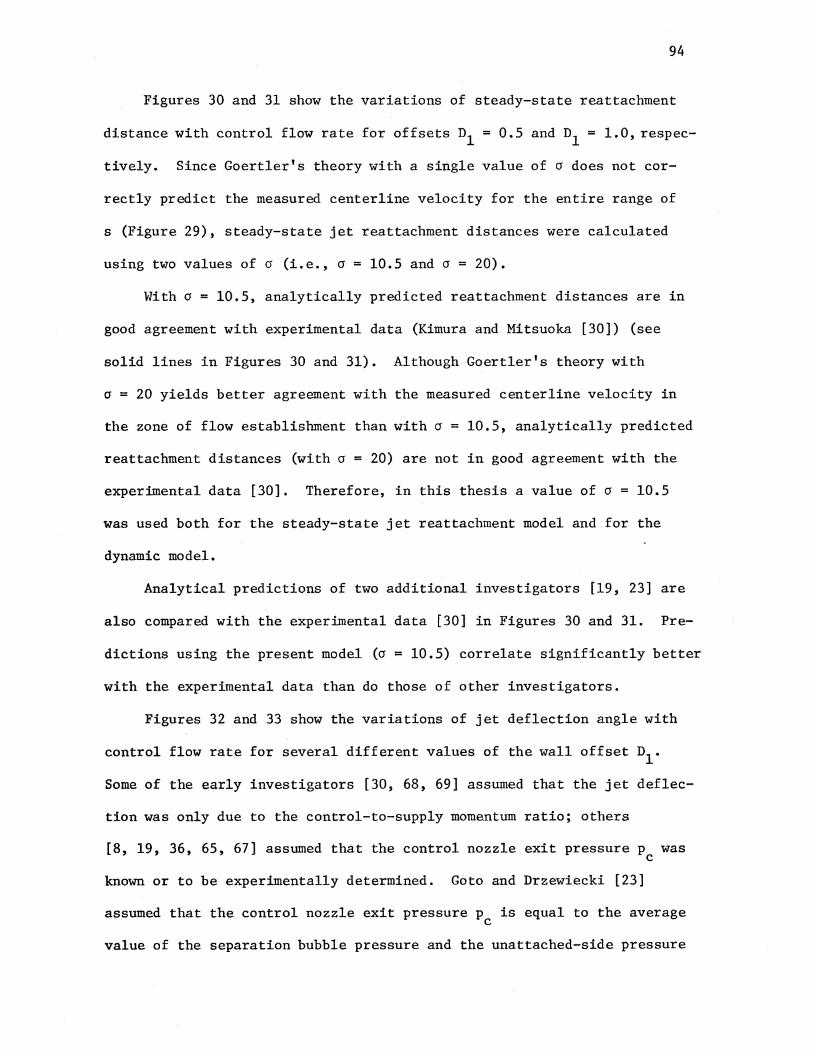
94
Figures 30 and 31 show the variations of steady-state reattachment
distance with control flow rate for offsets n1 = 0.5 and n1 = 1.0, respec
tively. Since Goertler's theory with a single value of a does not cor-
rectly predict the measured centerline velocity for the entire range of
s (Figure 29), steady-state jet reattachment distances were calculated
using two values of a (i.e., a= 10.5 and a= 20).
With a = 10.5, analytically predicted reattachment distances are in
good agreement with experimental data (Kimura and Mitsuoka [30]) (see
solid lines in Figures 30 and 31). Although Goertler's theory with
a = 20 yields better agreement with the measured centerline velocity in
the zone of flow establishment than with a = 10.5, analytically predicted
reattachment distances (with a = 20) are not in good agreement with the
experimental data [30]. Therefore, in this thesis a value of a= 10.5
was used both for the steady-state jet reattachment model and for the
dynamic model.
Analytical predictions of two additional investigators [19, 23] are
also compared with the experimental data [30] in Figures 30 and 31. Pre-
dictions using the present model (a = 10.5) correlate significantly better
with the experimental data than do those of other investigators.
Figures 32 and 33 show the variations of jet deflection angle with
control flow rate for several different values of the wall offset n1 •
Some of the early investigators [30, 68, 69] assumed that the jet deflec-
tion was only due to the control-to-supply momentum ratio; others
[8, 19, 36, 65, 67] assumed that the control nozzle exit pressure pc was
known or to be experimentally determined. Goto and Drzewiecki [23]
assumed that the control nozzle exit pressure p is equal to the average c
value of the separation bubble pressure and the unattached-side pressure
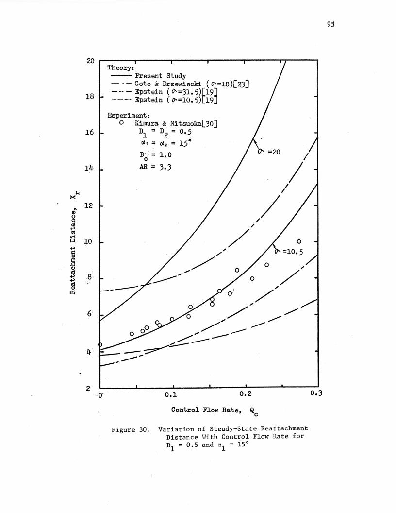
20
18
16
14
><~
·12 .. Cl) 0
~ ~ ..-1 ~ 10 ~
tij .E 0 cd ~ -~ i p;;
6·
2 . <r
Theory: Present Study
- -- Goto & Drzewiecki ( <7'=10 )[23] ---- Epstein ( 0'=31..5)[19] ---- Epstein ( 0'-=10 • .5)[19]
Esperiment: 0 Kimura & Mitsuoka[30]
D1 = D2 = 0 • .5
0(1 = ti.z = 1.5o
B· = 1~ 0 c • AR = 3.3
0.1 0.2
Control Flow Rate, Q c
Figure 30. Variation of Steady-State Reattachment Distance \-lith Control Flow Rate for D1 = 0.5 and a1 = 15°
95
0.3

20
18
16
14
J.f ><
12 .. 0> 0 s:= CIS
+> (/)
;::: 10
~ 0>
.2 0 CIS
8 +>
i p:;
6
4
2 0
Theory: -- Present Study - -- Goto & Drzewiecki (cr- =10)[23] ---- Epstein (o--=31.5)[19] --- Epstein ( cr- =10. 5)[19]
Experiment: ~ Kimura & Mitsuoka[30]
D1 = D2 = 1.0 0
o(. = c/.2. = 15
B = 1.0 c AR = 3.3
~/ ,/
96
,
,/
~-/ ----------- -~.::_ __ -----
....
0.1 0.2
Control Flow Rate, Q c
Figure 31. Variation of Steady-State Reattachment Distance With Control Flow Rate for D1 = 1.0 and a1 = 15°
0.3
0.4
0.3
0.2
.. Q)
1 s:: 0.1 0
..-1 -f-) 0 Q)
0 Q)
A
~ 0 1-)
0.1
0.2
Theory: Present Study (o-- =10. 5)
--- Goto & Drzewiecki (o-- =10.0)[23] --- Momentum ratio [30,68,69]
Experiment: 0 Lush (Figure(VIII.31) of [36])
D1 = D2 = 0.482
cJ. I : o( l- : 15 °
L--------
0 0.1
/ /
/
/ /
0.2 0.3
Control Flow Rate, Q c
0.4
Figure 32. Variation of Jet Deflection Angle With Control Flow Rate for D1 = 0.482 and a = 15°
1
97
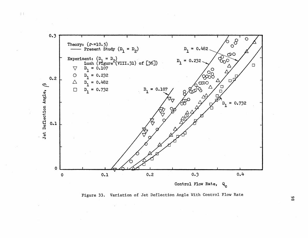
I I
~ .. Q)
i < s::: 0
oM +l () Q)
q Q)
J=l
+l Q)
t-:1
0.3
0.2
0.1
Theory: (0'=10. 5) -- Present Study (D1 = D2)
Experiment: (D = D2) Lush (i1:gure (VIII. 31) of [36])
'\7 D1 = 0.107
0 D1 = 0.232
D. D1 = 0.482
0 D1 = 0,732
0.732
0 I I I 6yr 4,) I~ I I I I I J
0 0.1 0,2 0.3
Control Flow Rate, Q c
0.4
Figure 33. Variation of Jet Deflection Angle With Control Flow Rate "" 00

99
(i.e., pc = (p1 + p2)/2); consequently, the value of pc was always nega
tive for any control flow rate. Lush [36] showed in static pressure
measurements at the control nozzle exit plane that the value of p is c
positive for Qc > 0.11 and D1 = 0.107, or for Qc > 0.22 and D1 = 0.482.
As shown in Figure 32, analytical predictions of other investigators
[23, 30, 68, 69] do not agree well with the experimental data of Lush
[36; Figure (VIII.31)].
The value of minor loss coefficient ~ used in the present model was
chosen to be unity by matching a predicted jet deflection angle with a
particular measured value [36; Figure (VIII.31)] for Qc = 0.25 and D1 =
0.482. However, as shown in Figures 32 and 33, the present model predic-
tions agree well with the experimental data [36] for the entire range of
the control flow rate used, and for the wall offset D1 of 0.107 to 0.732.
The computer execution time for an analytical prediction (i.e., for
each point on each curve) in Figures 30 through 33 on an IBM 370/158 was
of the order of 0.4 second.
5.3 Comparison of Dynamic Model Predictions
With Experimental Data
Figure 34 shows a comparison between analytically predicted switch-
ing times and the author's experimental data for the monostable fluid
amplifier with the nominal geometry. For these predictions and measure-
ments the amplifier input (control total pressure, hereafter called con-
trol pressure) was a terminated ramp-type signal with a preselected
saturation level. The measured control input rise time (from the first
discernible change in the initial control pressure to the final value P ) tc
was between 2 and 3 milliseconds. For the analytical prediction, the

12
10
8 C\l I 0 ,.;
><
~V) 6
.. Cl) !':; oM 8 bD r:: :E 4 () .p oM
~
2
0
0 Theory (0'= 10.5)
0 Experiment: D1 = 0.5
0 n2 = 1.0.
Bb = 2.0
e D =11.0 0 s
'C's = ts/tt
tt = b /u = 4.33 x 10⁻² ms s s
0
e 0
0.2 0.4 0.6 0.8 1.0
Final Value of Control Pressure, P tc
Figure 34. Variation of Switching Time With Control Pressure for the Monostable Fluid Amplifier With the Nominal Geometry
100
101
rise time was assumed to be 2. 5 milliseconds. The, effect of the rise
time variations (+0.5 millisc.cond) on the analytical prediction was +0.6
percent of full scale (i.e., in this case, T = 1200).
The agreement between theory (with a = 10.5) and experiment in
Figure 34 is excellent except for the low control pressure range. For
control pressures less than P = 0.4, corresponding switching times are tc
1 d b "l" 2 f h . arge an repeata 1 1ty o t e measurements l.S poor. Because of this
poor repeatability and large switching time, the use of control pressure
below P = 0.4 is not practical in the application of the monostable tc
amplifier.
Figure 35 shows a comparison between analytically predicted return
times and experimental data for the monostable fluid amplifier with the
nominal geometry. The control pressure was initially applied to the con-
trol chamber and then "suddenly" removed from the c·hamber by closing the
solenoid valve. When the solenoid valve was closed!,. the inlet to the
control chamber was open to the ambient. The meamJJred control input
decay time (from the first discernible change in ~he control pressure P tc
to an ambient pressure) was between 1 and 2 milliseconds. In the analy-
tical predictions, the decay time was assumed to be 1.5 milliseconds.
The effect of decay time variations (± 0.5 millise£'ond) on the analytical
predictions was ± 1.2 percent of reading.
The experimental results (Figure 35) show that the effect of the
initial control pressure level on the return time :is negligible. This
is expected since return to the attachment wall its; governed mainly by the
flow through the bias vent port after the control ]!l'ressure decreases be-
low a "threshold value." However, the analytical wrediction of the return
time is slightly affected by the initial value of '!the control pressure.

102
10
8
C\1 0 0 8 cs 'o 8 ..... 8 § 0
X 6 0 0 0
~!....
.. Q)
s 4 ..-f
8
~ Theory (rr- =10. 5) ~
~ 0 Experiment:
2 D1 = 0.5
D = 2
1.0
Bb = 2.0
D = 11.0 s
0 0.2 0.4 0.6 0.8 1.0
Initial Value of Control. Pressure, Pte
Figure 35. Variation of Return Time With Control Pressure for the Molmstable Fluid Amplifier With the Jnbminal Geometry
103
The analytical predictions exhibit a maximum error of 20 percent of read
ing3 over the range of the control pressure tested.
Figure 36 shows the effect of the jet spread parameter (a) variation
on the analytical predictions of the switching time for the monostable
amplifier. The effect is not significant in the range of 10.5 <a< 20 for
P > 0.4. A change in a from 10.5 to 7.7 causes a significant increase tc
in the "threshold value" of the control pressure (below which no switch-
ing occurs). A value of a= 20 gives better correlation with the mea-
sured switching times for P < 0.7, than does a= 10.5. However, in the tc
present study a value of a = 10.5 was used for the dynamic model because
(1) the steady-state jet reattachment model with a = 20 cannot correctly
predict the jet reattachment distance (see the discussion in section 5.2),
and (2) the control pressure range of practical interest is P > 0.4. tc
Figure 37 shows a comparison between analytically predicted switch-
ing times (using the present model) and the experimental data of Goto and
Drzewiecki [23] 4 for a bistable fluid amplifier. The dimensions of the
Goto and Drzewiecki test model is given in Table II, along with the dimen-
sions of the Lush test model. The rise time in the referenced experiment
was between 1 and 2 milliseconds. A rise time of 1.5 milliseconds was
assumed for the analytical prediction; Goto and Drzewiecki [23] also used
this rise time.
Goto and Drzewiecki defined the switching time as the time elapsed
from the first discernible change in the control pressure until the hot-
film probe located at the point of the splitter registered the maximum
signal. For the analytical prediction it was assumed that the hot-film
probe registered the maximum signal just before tl1e jet reattached to the
opposite wall (i.e., at the end of phase I). The agreement between the

12
10
8 N I 0 ...-l
~
til 1-'
"' Q) 6 !! E-1
00 ~
•.-I ,.c CJ +J o.-1 4 ::= til
2
0 0.2
I I Theory:
~ I
(!'- = 7.7 (/"' =10.5
I (/"' =20.0
I . ·o Experiment: I I D1 = 0.5
~ I
I I n2 = 1.0
I Bb = 2.0
I D = 11.0 s I I
\ I I
\0 I
~ I
0.4 0.6 0.8 Final Value of Control Pressure, P tc
--
1.0
Figure 36. Effect of Jet Spread Parameter (a) Variation on the Switching Time for the Monostable Fluid Amplifier
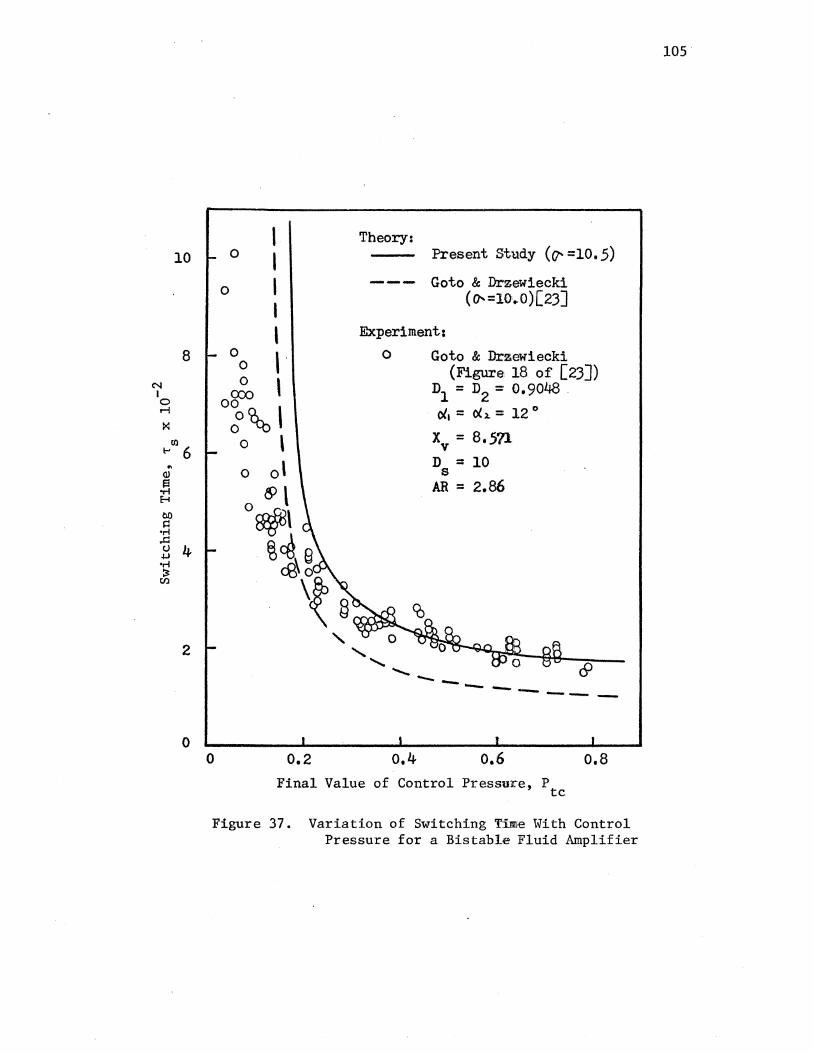
N I 0 r-i
X
10
8
Cl)
1-' 6
2
0 0
0 0
0 0
I I I I I
' ' ~' 0:0~'
0 \ 0
0.2
Theory: Present Study (0"' =10. 5)
--- Goto & Drzewiecki ( cr- =10. 0 )[23 J
Experiment:
0 Goto & Drzewiecki (Figure. 18 of [23])
D1 = D2 = 0.9048 .
0.4
<X. = ex~ = 12 o
X = 8 • .571 v D = 10 s AR = 2.86
0.6 o.8 Final Value of Control Pressure, P
tc
Figure 37. Variation of Switching 'I'i:mrre With Control Pressure for a Bistable Fluid Amplifier
105
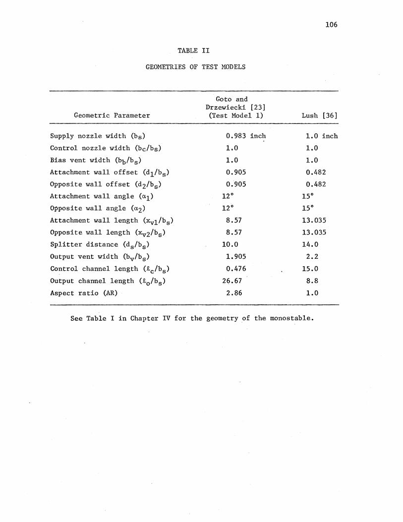
TABLE II
GEOMETRIES OF TEST MODELS
Geometric Parameter
Supply nozzle width (bs)
Control nozzle width (bc/bs)
Bias vent width (bb/bs)
Attachment wall offset (d1/bs)
Opposite wall offset (d2/bs)
Attachment wall angle (al)
Opposite wall angle {a2)
Attachment wall length (Xvllbs)
Opposite wall length <Xv2/bs)
Splitter distance (ds/bs)
Output vent width (bv/bs)
Control channel length (ic/bs)
Output channel length (i0 /bs)
Aspect ratio (AR)
Goto and Drzewiecki [23] (Test Model 1)
0.983 inch
1.0
1.0
0.905
0.905
12°
12°
8.57
8.57
10.0
1.905
0.476
2~.67
2.86
106
Lush [36]
1.0 inch
1.0
1.0
0.482
0.482
15°
15°
13.035
13.035
14.0
2.2
15.0
8.8
1.0
See Table I in Chapter IV for the geometry _of the monostable.

present model predictions and the experimental data is very good for
Pte > 0.25 and superior to that due to Goto and Drzewiecki.
107
Figure 38 shows a comparison between analytically predicted switch
ing times and the experimental data of Lush [36] 5 for a bistable fluid
amplifier. The dimensions of the Lush test model is given in Table II.
Lush reported that the static pressure and flow rate just upstream of
the control nozzle exit plane took the order of 20 milliseconds to rise
to their steady value. For the analytical prediction in Figure 38, the
rise time of the total pressure at the inlet of the control channel was
calculated by considering the inertance and resistance of the channel so
that the rise time of the flow rate at the control nozzle exit plane was
20 milliseconds.
Lush defined the experimental switching time as the time elapsed
from the first discernible change in the control pressure until the total
pressure probe located at the end of the opposite wall registered a maxi
mum signal. (The total pressure probe was positioned so that it was near
tp the jet centerline after switching had finished.) For the analytical
prediction it was assumed that the probe registered a maximum signal at
the beginning of phase II.
Although Lush obtained data from a test amplifier which had an aspect
ratio of unity, the prediction using the present model is still in good
agreement with his data except for the low control pressure range.
Figure 39 shows a comparison of an analytically predicted NOR output
total pressure transient response with an experimentally measured one. A
"negative step" input signal having a decay time of 1.5 milliseconds
approximates the experimental input condition. The present modelpredicts
the overall transient response reasonably well, even though the predicted

C"' I 0 r-1
~
(/) !-'
"' (])
s •r-l E-1
00 $:1
•r-l ,.r.:: tJ -1-' •r-l )
Cl)
8 ....,
I Theory: 0 I I
--- Present Study (l7' =10.5) 0
7 - I Experiment:
I 0 Lush (Figure(VIII.6) of [36])
' D1 = D2 = 0.4821
6 1- 0 ' 0(,= ()(}. = 15 Cl
\ X = 13.035 \ v
<9 D = 14.0 \ 0 s
5 0 AR = 1.0 .. \
0 \ co \ 4 - \
\ co o\
3 - \0
\ 'b,
'-Q -2 ....... ......... o'...._ 0 ...._ ---
1 I'"
0 I I I I I
0.2 0.3 0.4 0.6
Final Value of Control Pressure, P tc
Figure 38. Variation of Switching Time With Control Pressure for a Bistable Fluid Amplifier
108
0.8
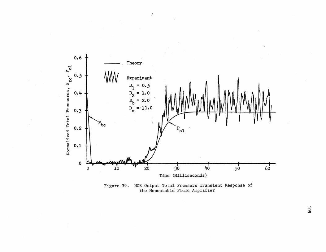
0.6 .-l 0 p..
.. o.s t) .j.J
p..
.. (/) 0.4 (J) 1-1 ;:! (/) (/) (J)
1-1 O.J p..
.-l cu .j.J
0 E-1 0.2 "0 (J) N
•r-l .-l cu 0.1 13 1-1 0 z
0
.
1\
Theory
WN Experiment
D1 = 0.5 n2 = 1.0
Bb = 2.0
D = 11.0 s
"pte
JO 40 50 Time (Milliseconds)
Figure 39. NOR Output Total Pressure Transient Response of the Monostable Fluid Amplifier
60
I-' 0
""

110
final value of the total pressure is 15 percent less than the measured
mean value.
The noise in the measured output response in Figure 39 is mostly due
to the turbulence of the jet. The value of the turbulence intensity
•2 (u 2 ; U01 = mean velocity at the output exit plane) measured at the NOR uol
output channel exit plane was of the order of 0.014. In contrast, the
u'2 maximum value of a semi-confined jet turbulence intensity (--2- ; u =
uc c
jet centerline velocity) reported in References [7, 25, 28] is of the
order of-0.083.
Figure 40 shows the predicted effect of the control input pressure
"shape" on the OR output total pressure transient response of the mono-
stable fluid amplifier. Two control input pressures of different shapes
are used for the analytical predictions: one (dashed line) is a termi-
nated ramp-type input. signal having a rise time of 2. 5 milliseconds and
the other (solid line) is an exponential input signal having a time con-
stant of 10 milliseconds. Both control pressures have the same initial
value of -0.154 and final value of 0.41. The output response time (or
switching time) for the exponential input signal is almost twice as long
as that for the terminated ramp-type input signal. Although the predicted
output responses are not validated by experiment, it is expected that they
are valid within the range of error which the predicted NOR output re-
spouse exhibits (see Figure 39).
The computer simulation time for an analytical prediction (e.g., a
switching time for a given control pressure) on an IBM 370/158 was of the
order of 15 seconds.

C) ~
P-1
"' <I) ,_, :::1 00 00 <I) ,_,
P-1
M 0 ,_, ~ t=: 0 u "1j
Q) N
'M M
~ ,_, 0 z
0.6 - O.J,... Po2
N ~--------0
/"" ·.
P-1 r_L::_c ___ i ______ "' 0.4
<I) 0.2 ,_,
::l 00 I I 00 <I) ,_,
P-1 I M tO
I I /'P+r- = 0.564(1-e-t/0.01)-0~154 ~
0.2 0 0.1 I H
I ~
:::1 I 0. I ~ :::1 I 0 I D = 0.5
"1j I 1
Q) D2 = 1.0 0
N 0 / 'M M tO Bb = 2.0 s ,_, 0 D s = 11.0 z
0, 2 L 0,1 '-----'-------lt------'------ll..----...:.L..---.-J 0 10 20 JO 40 50
Time (Milliseconds)
Figure 40. Predicted Effect of Control Input Pressure Shape on the OR Output Total Pressure Transient Response of the Monostable Fluid Amplifier
60
f-l f-l f-l
112
5.4 Experimental Data Repeatability
The scatter of the experimental data shown in Figures 34 through 36
was due to: (1) the variation o.f the control pressure rise (or decay)
time, (2) the difficulty of measuring the mean value from the output velo
city trace, and (3) the nature of the fluid dynamic process inside the
monostable fluid amplifier. The scatter in the switching and return time
data for low control pressures was due mainly to the latter effect as ex
plained below.
Experimental studies [36, 63] have shown that the growth rate of the
separatio.n bubble decreases after the reattachment point reaches the out
put vent edge (point K, in Figure 15b), because of the reduced return flow
into the bubble. If the control flow is not large enough to make the jet
"jump" over the output vent and attach to the wall downstream of it, then
a stable situation develops with the jet remaining at the end of the wall.
However, turbulent eddies traveling down the edges of the jet tend to de
stabilize the flow balance near the end of the wall and the jet may "jump"
over the output vent, depending on how close the control flow is to the
threshold value (below which no switching occurs). The poor repeatability
for low control pressures (see Figure 34) is probably due to this indeter
minate "dwell period" before the jet "jump" [36].
5.5 Effects of Geometric Variations on
Switching and Return Times
This section presents the results of experimental and analytical in
vestigations of the effects of geometric variations on the switching and
return times of the monostable fluid amplifier.
113
5.5.1 Effect of Attachment Wall Offset, Dl
Figure 41 shows the effects of varying attachment wall offset n1 on
the switching and return times of the monostable amplifier. The experi
mental results show that an increase in the offset D1 reduces the switch
ing time, but increases the return time greatly. Analytical predictions
also show the trend very well.
If a fast return and a fast switching time is taken as a criterion
for a "best" design of a monostable fluid amplifier, a "best" offset n1
may be obtained by observing the intersection of the two curves shown in
F~gure 41. That is, with this criterion n1 ;; 0.4 is the "best" geometry
in this study.
Poor repeatability of the measurements for an offset in the region
of D1 = 0.25 is probably due to the indeterminate ndwell period" before
the jet "jump" (see section 5.3 for detailed discussion).
5.5.2 Effect of Opposite Wall Offset, D2
Figure 42 shows the variation of switching time with opposite wall
offset, n2 . An increase in the offset n2 results in a great increase in
the measured switching time. Analytical predictions also show the trend
very well. Repeatability of the measurements is poor for offsets greater
than n2 = 1.0.
Figure 43 shows the variation of return time with offset n2 . The
experimental results show that the effect of varying n2 on the return
time is negligible in the range of n2 ~ 1. 5. But in the range of n2 < 1. 5
a decrease in the offset results in a great increase in the return time,
because the reduced passage between the jet edge and the opposite wall
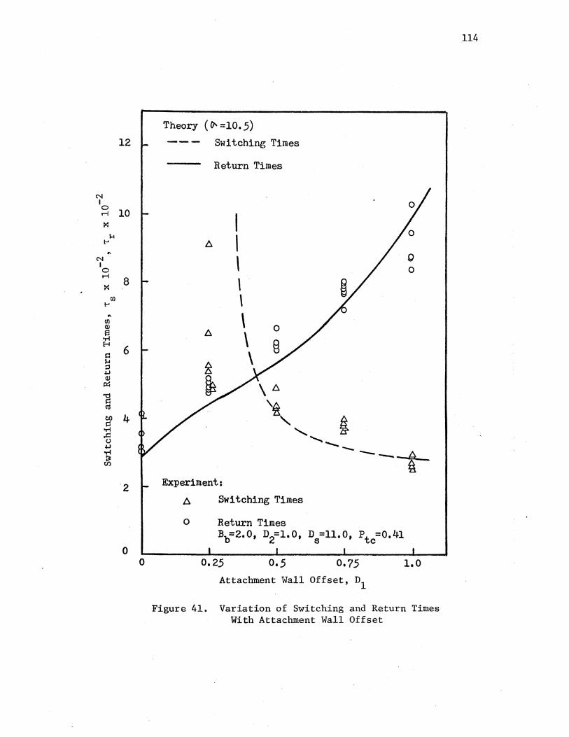
N I
12
~ 10 :><:
N I 0 r-1
:><:
Cll 1-'
8
2
0 0
Theory ( 0.. =10. 5)
Switching Times
Return Times
Experiment:
I
' \ \ \ \ \ \
0
A Switching Times
o Return Times Bb=2.0, D2=1.0, Ds=11.0, Ptc=0.41
0.25 0.75 Attachment Wall Offset, n1
Q
0
1.0
Figure 41. Variation of Switching and Return Times With Attachment Wall Offset
114
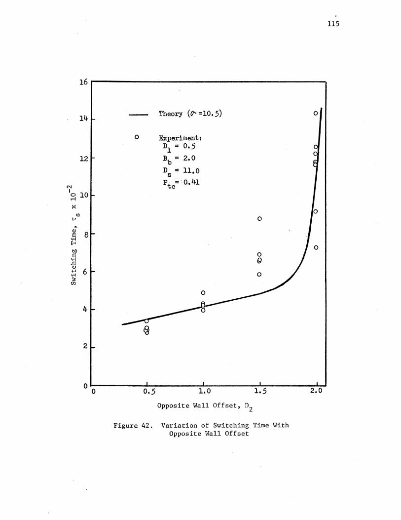
16r-----------------------------------------
14 Theory (0' =10. 5) 0
0 Experiment: D1 = 0.5
12 Bb = 2.0
D = 11 0 s •
N Pte=· 0.41
I 0 10 r-1
X 0
{/)
0 !-' .. aJ
~ E-1
00 1=1 Tl ,.c: t.l +J •.-I :.>:
Cl)
8
0
6
4
2
0~--------~----------~--------~----------~~ 1.5 1.0 2.0 0 0.5
Opposite Wall Offset, D2
Figure 42. Variation of Switching Time With Opposite Wall Offset
115
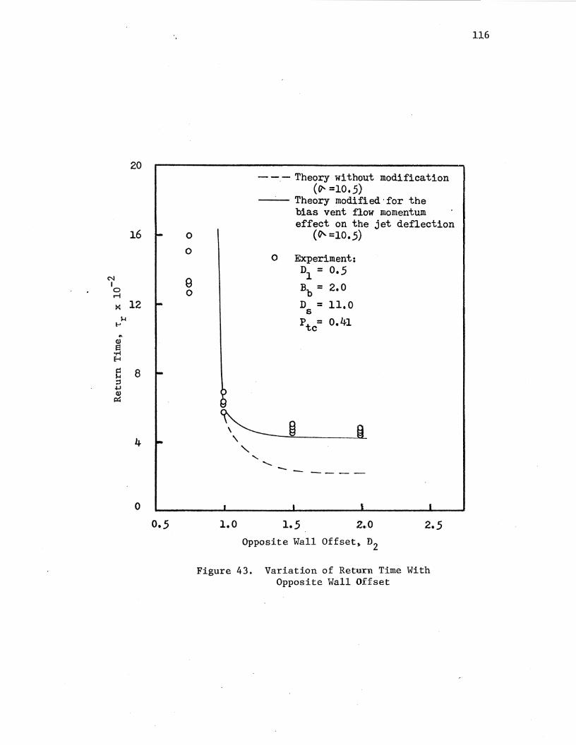
N I 0 ,.....j
><:
l-1 !-' .. Q) s
•r-1 E-1
s::: l-1 ;:I -1.1 Q)
p::
20
16
12
8
4
0
0.5
0
0
e 0
1.0
--- Theory without modification (If' =10.5)
-----Theory modified·for the bias vent flow momentum effect on the jet deflection
(~=10.5)
0 Experiment:
-
D1 = 0,5
Bb = 2.0
D = 11.0 s Pte= 0,41
-----
1.5 2.0
Opposite Wall Offset~ D2
2.5
Figure 43. Variation of Return Time With Opposite Wall Offset
116

(~ in Figure 44) restricts the induced flow from the bias vent port.
For n2 < 0.75, there is no return at all; that is, the jet remains
attached to the opposite wall.
117
If the passage ab is greater than bias vent width bb, the momentum
(Jb) of the induced flow from the vent is no longer parallel to the jet
centerline (see Figure 44). Therefore, Equations (3.73) and (3.75),which
are derived from the momentum balance in the control volume (Figure 44),
need to be modified. A simple modification has been made empirically.
With a 36 percent reduction in the momentum flux of the bias vent flow, 6
the present model (with cr = 10.5) can predict the return time within 6
percent of the measured value for n2 > 1 (see the solid line in Figure
43).
For n2 < 1 the present model (with cr = 10.5) can only show the
general trend. However, an offset less than unity is not important in
the practical design of the monostable amplifier because of the large
return time.
If a fast return and a fast switching time is taken as a criterion
for a "best" design of a monostable fluid amplifier, a "best" offset n2
can be obtained in a way similar to that discussed in section 5.5.1.
That is, with this criterion n2 ; 1. 2 is the "best:" geometry in this
study.
5.5.3 Effect of Splitter Distance, Ds
Figure 45 shows the variation of switching time with splitter dis-
tance D • The effect of varying the splitter distance on the measured s
switching time is negligible in the range of 10.5 < D < 13. An increase s
in a splitter distance over D = 13 results in a great increase in the s
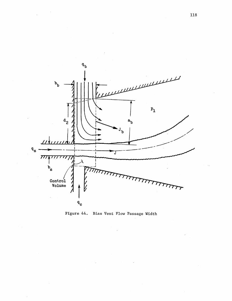
qs -~~----+----
Control Volume
t Figure 44. Bias Vent Flow Passage Width
118

119
20
Theory ( 0'=10.5)
16 ~ 0 Experiment: 0
D1 = 0.5 0
N D2 = 1.0 I 0
B = 2.0 0 ..-I b
>4 12 - xv1 = 10.94 0 til
1-' p = 0.41 .. tc
Q)
~ 0 H
bO 0 0 ~ 8 •r-1 -..c:
t) ~ 8 g or-! ~
U) s
fl 0 0 0
Q [).. 0 Q 8 4 ~ "{) v - 0
0 I I l ' 10 11 12 lJ 14
Splitter Distance, D s
Figure 45. Variation of Switching Time With Splitter Distance
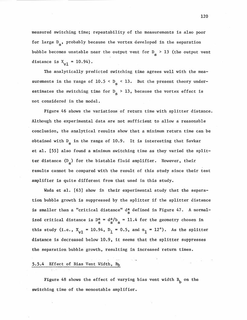
120
measured switching time; repeatability of the measurements is also poor
for large D , probably because the vortex developed in the separation s
bubble becomes unstable near the output vent for D > 13 (the output vent s
distance is xvl = 10.94).
The analytically predicted switching time agrees well with the mea-
surements in the range of 10.5 < D < 13. But the present theory unders
estimates the switching time for D > 13, because the vortex effect is s
not considered in the model.
Figure 46 shows the variations of return time with splitter distance.
Although the experimental data are not sufficient to allow a reasonable
conclusion, the analytical results show that a minimum return time can be
obtained with D in the range of 10.9. It is interesting that Savkar s
et al. [55] also found a minimum switching time as they varied the split-
ter distance (D ) for the bistable fluid amplifier. However, their s
results cannot be compared with the result of this study since their test
amplifier is quite different from that used in this study.
Wada et al. [63] show in their experimental study that the separa-
tion bubble growth is suppressed by the splitter if the splitter distance
is smaller than a "critical distance" d* defined in Figure 47. A normals
ized critical distance is D* = d*/b = 11.4 for the geometry chosen in s s s
this study (i.e., Xvl = 10.94, n1 = 0.5, and a1 = 12°). As the splitter
distance is decreased below 10.9, it seems that the splitter suppresses
the separation bubble growth, resulting in increased return times.
5.5.4 Effect of Bias Vent Width, Bb
Figure 48 shows the effect of varying bias vent width Bb on the
switching time of the monostable amplifier.

9
8
?
('I
I 0 ...... X
~ 6
1-'
.. ~
•.-! E-t
5 ~ ~ ;::l .j.J (!) ~
4
3
2 10
0
0 0,
Theory (fJ'o =10. 5)
Experiment: D1 = 0.5 D2 = 1.0
Bb = 2.0
Pte = 0.41
11 12
Splitter Distance, D s
Figure 46. Variation of Return Time With Splitter Distance
121
1.3

* d s
xvl -------J
I I I
I
I I
Figure 47. Critical Splitter Distance [63]
122

12
10
N 8-I 0 ...-!
~
Cl)
1-'
.. Q) 6 13
•r-1 E-1
bO ~
•r-1 .c: CJ oiJ •r-1 ~
tl) 4
-2
0 0.2
0
0
~
$
D. D.
I I I Theory (C7'=10.5):
I Bb = 2.0
I --- Bb = 1.5
\ Experiment: \ I 0 Bb = 2.0 I b /:::. Bb = 1.5
I D1 = 0.5 I I D2 = 1.0
I D = 11.0 I s I
' \_
o'
§\ /:::. \ \
0.4 0.6 0.8 Final Value of Control Pressure, P tc
1.0
Figure 48. Effect of Bias Vent Width on the Switching Time
123
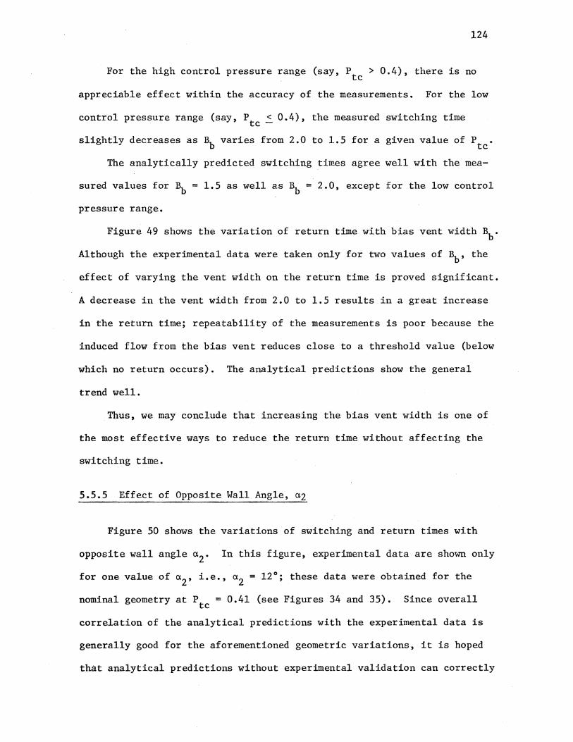
124
For the high control pressure range (say, P > 0.4), there is no . tc
appreciable effect within the accuracy of the measurements. For the low
control pressure range (say, P < 0.4), the measured switching time tc -
slightly decreases as Bb varies from 2.0 to 1.5 for a given value of P tc
The analytically predicted switching times agree well with the mea-
sured values for Bb = 1.5 as well as Bb = 2.0, except for the low control
pressure range.
Figure 49 shows the variation of return time with bias vent width Bb.
Although the experimental data were taken only for two values of Bb, the
effect of varying the vent width on the return time is proved significant.
A decrease in the vent width from 2.0 to 1.5 results in a great increase
in the return time; repeatability of the measurements is poor because the
induced flow from the bias vent reduces close to a threshold value (below
which no return occurs). The analytical predictions show the general
trend well.
Thus, we may conclude that increasing the bias vent width is one of
the most effective ways to reduce the return time without affecting the
switching time.
5.5.5 Effect of Opposite Wall Angle, a2
Figure 50 shows the variations of switching and return times with
opposite wall angle a 2 • In this figure, experimental data are shown only
for one value of a 2 , i.e., a 2 = 12°; these data were obtained for the
nominal geometry at P = 0.41 (see Figures 34 and 35). Since overall tc
correlation of the analytical predictions with the experimental data is
generally good for the aforementioned geometric variations, it is hoped
that analytical predictions without experimental validation can correctly
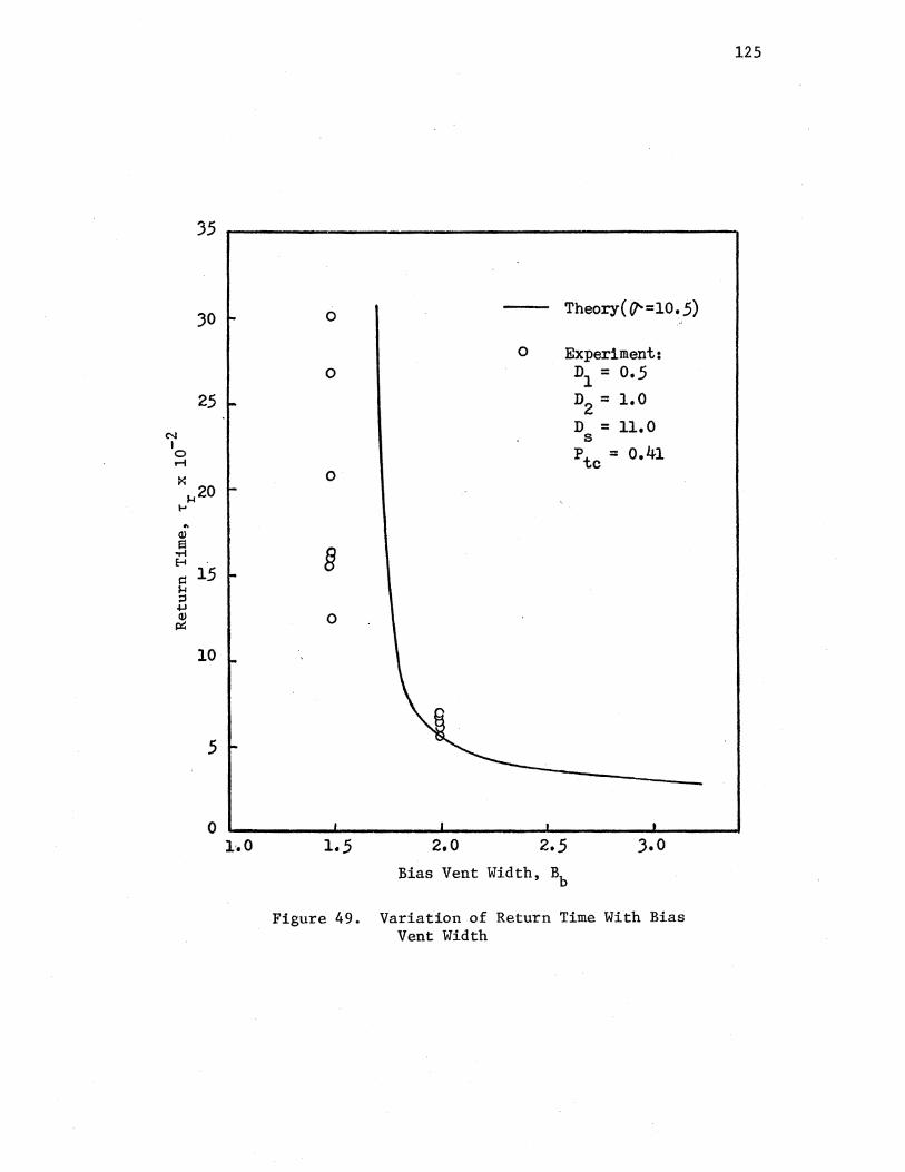
35
30
25
N I 0 .-I
~
l-l20 1-'
.. (l) s
-M E-i
l=l 1-l ;:I
.j...J (l) ~
15
10
5
0 hO
0 Theory( 0"'=10. 5)
0 Experiment: 0 D1 = 0.5
D2 = 1.0
D = 11.0 s Pte = 0.41
0
§
0
1.5 2.0 3.0
Bias Vent Width, Bb
Figure 49. Variation of Return Time With Bias Vent Width
125
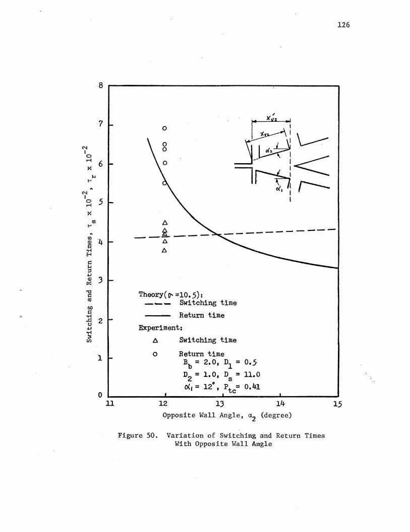
8
7
N I 0 r-1
6 ::< 1-1
!-'
N I
5 0 r-1
::< til
!-'
t
0 11
0
0 0
6
126
__ i_ __ _ _ ___ __._.-
6
A
Theory( fl" =10. 5): --- Switching time
Return time
Experiment:
A Switching time
0 Return time B = b
2.0, D = 1 0.5 D = 2
1.0, D = 11.0 s o<, = 12°' Pte= 0.41
12 13
Opposite Wall Angle, a2
14
(degree)
Figure 50. Variation of Switching and Return Times With Opposite Wall Angle
15

present the principal effects of varying a 2 and n3 (see next section)
on the switching and return times of the monostable amplifier.
When a 2 is varied, the following two ways are available to hold
other variables constant at the nominal geometry: (1) opposite wall
127
length xv2 is kept constant, or (2) output vent location is kept constant
(i.e., x~2 =constant; see the insert in Figure 49). The second way was
chosen in this study.
The effect of varying the opposite wall angle on the switching time
is negligible; however, an increase in the opposite wall angle results in
a substantial decrease in the return time. Thus, we may conclude that
this geometric change is another effective way to reduce the return time
without sacrificing the switching time.
5.5.6 Effect of the Splitter Offset, D3
Figure 51 shows the variations of switching and return times with
splitter offset n3 • In this figure the experimental data are shown only
for one value of n3 , i.e., n3 = 0; these data were obtained for the
nominal geometry at P = 0.41 (see Figures 34 and 35). tc
An increase in the splitter offset toward the opposite wall reduces
the switching time slightly. The effect of varying the splitter offset
on the return time is negligible for n2 < 0.2, but an increase in the
splitter offset over n3 = 0.2 results in the substantial increase in the
return time.
5.6 Limitation of the Model
Figure 52 shows the effect of output loading (blockage of OR output
channel) on the switching time. A 0.118 inch inside diameter orifice was

8
7
N I 0 r-1
6 ~
1-1 1-'
... N I 0 r-1 5 ~
Ul 1-'
1
0 0
------ ----- ._. ----- --...._ .... ---~· ._
Theory(cr- =10. 5): --- Switching time
Return time
Experiment: A Switching time
0 Return time Bb = 2.0, D1 = 0.5 D = 1.0, D = 11.0
2 s p = tc 0.41
0.1 0.2 0.3
Splitter Offset, n3
0.4
Figure 51. Variation of Switching and Return Times With Split-ter Offset
0 •. 5
128
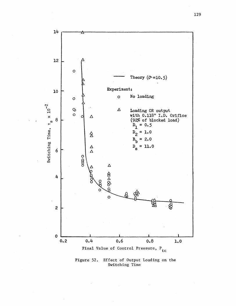
14
12
10
N I 0 r-1
X Ul 8
~ .. Q)
s •r-1 E-i
bO 1=1
•r-1 .t:: 6 C) 4-1 •r-1 ~
Cl.l
4
2
0 0.2
0
0
Q> 0
f).
Theory (0'-=10. 5)
Experiment:
0 No loading
Loading OR output 0 6 with 0.118" I.D. Orifice
(92.% of blocked load) D1 = 0.5
~ D =
2 1.0
Bb = 2.0
6. D = 11.0 D.
s
0
~
0.4 0.6 0.8 1.0 Final Value of Control Pressure, P tc
Figure 52. Effect of Output Loading on the Switching Time
129
130
mounted at the exit of the OR output channel; this resistance produced a
static pressure in the channel which was 92 percent of the blocked load
pressure recovery.
The switching time increases with OR output channel blockage. The
effect of the blockage is stronger at low control pressures than that at
high control pressures. However, in general, the effect of the blockage
depends on the geometry of the output vent and splitter. This effect can
be minimized or even eliminated by an appropriate design, such as employ
ing an output decoupling vent in the output channel [18].

ENDNOTES
1 See Chapter II for details.
2Repeatability of the experimental data is discussed in the next section.
3The average value of readings repeated five times at a given P was used for the error calculation. tc
4Among the several different experimental data sets they obtained, the data for the test model 1 (with splitter and inactive control open; Figure 18 of [23]) are chosen for this comparison. Since their data were normalized in a slightly different way from this study, they were replotted (Figure 37) with the following transformation: the control pressures are divided by (Cds)2 and the switching times are multiplied by Cds where Cds is the supply nozzle discharge coefficient (Cds = 0.85 was used by Goto and Drzewiecki [23]).
5Lush [36] measured the switching times for two different splitter distances (i.e., Ds = 14 and Ds = 20) of the bistable fluid amplifier. The experimental data for Ds = 14 (Figure (VII.6) of [36]) are chosen for this comparison because that geometry is more similar to the device used in the present study. Since Lush presented the measured switching times as a function of the jet deflection angle, his data were replotted (Figure 38) with the following transformation: Pte = 2S (from his expression for S; [36], p. 52).
6The reduction in the momentum flux of the bias vent flow may be obtained by substituting a modified bias vent flow Qb for Qb in Equations (3.73) and (3.75). The modified vent flow is given by
131

CHAPTER VI
SUMMARY, CONCLUSIONS, AND RECOMMENDATIONS
6.1 Summary
The jet centerline axial velocity distribution in the semi-confined
jet was measured to investigate the effect of the top and bottom plates
on the effective jet spread in the test amplifier. A value of the jet
spread parameter a in the region of 10.5 yields the best match with the
experimental data for s/b > 25. However, for a range of 4 < s/b < 15, s s
a = 20 yields a better match with the experimental data.
A steady-state jet reattachment model was developed which is capable
of accurately predicting the reattachment position of a two-dimensional,
incompressible, turbulent jet to an offset, inclined wall in the presence
of control flow. With a = 10.5, analytically predicted reattachment dis-
tances are in good agreement with experimental data due to Kimura and
Mitsuoka [30]. Based on this correlation and the measured jet centerline
axial velocity distribution, the value of a = 10.5 is established for the
present study. The analytically predicted jet deflection angles are also
in excellent agreement with Lush's experimental data due to Lush [36] for
attachment wall offsets of 0.107 ~ D1 ~ 0.732.
Based on the steady-state jet reattachment model, an analytical
dynamic model was developed which is capable of predicting the switching
time, the return time, and the transient response of a monostable fluid
amplifier to any time-varying input signal. The analytically predicted
132

133
switching times are within 10 percent of measured values except for the
low control pressure range. The analytically predicted return times are
within 20 percent of measured values over the range of the control pres-
sure tested for the nominal configuration of the monostable amplifier.
Correlation of the analytical predictions with the published experi-
mental data for a bistable fluid amplifier is also very good except for
the low control pressure range.
The NOR output total pressure transient response to a "negative
step" in control pressure (with finite decay time) was measured and com-
pared with an analytically predicted response. The dynamic model predicts
the output response reasonably well, even though the predicted final out-
put total pressure is 15 percent less than the measured mean value. The
OR output total pressure transient responses to control input pressures
of two different shapes (i.e., a terminated ramp-type and an exponential
type) were simulated to demonstrate the versatility of the present model
and to show the effect of control input pressure shape on the switching
time and the output transient response of the monostable amplifier.
The effect of the jet spread parameter (cr) variation on the predicted
switching time was studied. It was found that the effect is not signifi-
cant in the range of 10.5 < cr < 20 for P > 0.4. A change in cr from 10.5 tc
to 7. 7 causes a significant increase in,the predicted "threshold value" of
the control pressure.
The effects of geometric variations on the switching and return times
were studied experimentally and analytically (see Figure 27 for the geo-
metry). A summary of the results follows:
1. Attachment wall offset, n1 : An increase in the offset n1 reduced
the switching time, but increased the return time greatly. If a fast
return and a fast switching time is taken as a criterion for a "best"
design of a monostable fluid amplifier, a "best" offset n1 can be ob
tained.
134
2. Opposite wall offset, D2 : An increase in the offset D2 reduced
the return time, but increased the switching time greatly. For D2 > 1. 5,
the offset D2 variation had a negligible effect on the return time.
There was no return for D2 <0.75. If a fast return and fast switching
time are taken as criteria for a "best" design of a monostable fluid
amplifier, a "best" offset D2 can be obtained.
3. Splitter distance, D : With the splitter located near the outs
put vent (i.e., D = 10.9; X 1 = 10.94), a minimum return time was pre-s v
dieted and "stable" switching was observed experimentally. But the
splitter distance variation had a negligible effect on the measured
switching time for 10.5 < D < 13. s
4. Bias vent width, Bb: An increase in the vent width Bb reduced
the return time greatly. But the vent width variation had a negligible
effect on the switching time. Thus, increasing the bias vent width is
one of the most effective ways to reduce the return time without sacri-
ficing the switching time.
5. Opposite wall angle, a 2 : An increase in the angle a 2 reduced
the return time greatly, but the angle a 2 had a negligible effect on the
switching time. Thus, increasing the opposite wall angle is another
effective way to reduce the return time without affecting the switching
time.
6. Splitter offset, n3 : An increase in the offset D3 reduced the
switching time slightly. The offset variation had a negligible effect

135
on the return time for n3 < 0.2, but increasing n3 over 0.2 resulted in
an increase in the return time.
A limited experimental study was conducted to investigate the effect
of the output (OR) loading (blockage) on the switching time of the mono
stable amplifier. It was found that the effect of loading is stronger at
low control pressures than that at high control pressures. However, in
general, the effect of output loading depends on the geometry of the out
put vent and the splitter, and can be minimized or even eliminated by an
appropriate design of the amplifier (e.g., by employing an output decoup
ling vent shown in Reference [18]).
6.2 Conclusions
The analytical dynamic model has been shown to be capable of predict
ing not only the switching and return times but also the transient
response of a monostable fluid amplifier to any time-varying control input
signal. This model can be utilized as an analytical design tool for a
monostable fluid amplifier. This model can also be used in the simulation
of digital fluidic circuits.
The steady-state jet reattachment model has also been shown to be
capable of predicting the reattachment position of a two-dimensional, in
compressible, turbulent jet to an offset, inclined wall in the presence
of control flow. This steady-state model can be used to determine the
attachment and opposite wall lengths1 (defined in Figure 27 and Table I)
for the design of a monostable fluid amplifier.
The results obtained from the study of effects of geometrical varia
tions on the switching and return times for the test monostable amplifier

should be usable as a general guide in the design of monostable fluid
amplifiers.
136
The steady-state jet reattachment model and the dynamic model are
also applicable to a bistable fluid amplifier. The dynamic model should
also be useful in identifying the digital data handling speed of wall
attachment fluid amplifiers and in detecting hazards in digital fluidic
systems employing such amplifiers.
6.3 Recommendations for Future Study
The following areas are recommended for future study:
1. An input vent port (see Figure 5) is usually provided for con
trol input signal isolation in a wall-attachment fluid amplifier. The
static and dynamic characteristics of the control flow in the input vent
should be studied to broaden the range of application of the present
dynamic model.
2. The effect of the aspect ratio (AR) on the semi-confined jet
spread (i.e., cr) should be studied for AR < 6.
3. The effect of perpendicularly impinging control flow on the sup
ply jet spreading (i.e., cr) should be studied experimentally.
4. The assumption on the dynamic pressure at the inlet of the OR
and NOR output channels should be validated by experiment.
5. The criterion for the end of phase I should be further investi
gated.
6. Error in the final value of the output total pressure should be
investigated.
7. Further experimental study should be done to investigate the
effects of varying the opposite wall angle and the splitter offset on the
switching and return times of a monostable fluid amplifier.

ENDNOTE
1 The walls must be long enough so that when the control port is open to ambient pressure, the steady-state jet reattachment position is on the upstream side of the output vent. The following relation was suggested by Drzewiecki [18]:
Wall length = Steady-state jet reattachment distance+ 2b • s
137
BIBLIOGRAPHY
1. Abramovich, G. N. The Theory £i Turbulent Jets. Cambridge: The M.I.T. Press, 1963.
2. Bain, D. C. and P. J. Baker. Technical and Market Survey of Fluidics in the United Kingdom. Cranfield: The British Hydromechanics Research Association, 1969.
3. Bermel, T. W. and W. R. Brown. "Development of a Pure Fluid NORGATE and a NORLOGIC Binary to Decimal Converter." Fluid Amplification Symp. Proc., 3 (1965), pp. 37-61.
4. Boucher, R. F. "Incompressible Jet Reattachment Using a Good Free Jet Model." Third Cranfield Fluidics Conf. Proc., Paper Fl, 1968.
5. Bourque, C. and B. G. Newman. "Reattachment of a Two Dimensional Incompressible Jet to an Adjacent Flat Plat." Aeronautical Quart., 11, 3. (August, 1960), pp. 201-232.
6. Bourque, C. "Reattachment of a Two Dimensional Jet to an Adjacent Flat Plate." Advances in Fluidics. Ed. F. T. Brown. New York: ASME, 1967, pp. 192-204.
7. Bradbury, L. J. S. Plane Jet."
"The Structure of a Self-Preserving Turbulent ~· Fluid Mech., 23 (1967), pp. 31-64.
8. Brown, E. F. and F. C. Belen, Jr. "Jet Interaction in a Simplified Model of a Bistable Fluid Amplifier." ASME Paper 72-WA/Flcs-6, 1972.
9. Brown, F. T. "Pneumatic Pulse Transmission with Bistable Jet Relay Reception and Amplification." (Unpub. Sc.D. dissertation, Massachusetts Institute of Technology, 1962.)
10. Comparin, R. A., H. H. Glaettli, A. E. Mitchell, and H. R. Mueller. "On the Limitations and Special Effects in Fluid Jet Amplifiers." ASME ~· on Fluid Jet Control Devices, 1962, pp. 65-73.
11. Conway, A., ed. A Guide to Fluidics. London: McDonald, 1971.
12. Doble, P. A. C. and J. Watton. "Multiple Regression Analysis of Fluidics OR-NOR Elements." Fourth Cranfield Fluidics Conf. Proc., Paper X4, 1970.
138
139
13. Dodds, J. I. "The Use of Suction or Blowing to Prevent Separation of a Turbulent Boundary Layer." (Unpub. Ph.D. dissertation, University of Cambridge, 1961.)
14. Douglas, J. F. and R. S. Neve. "Investigation into the Behavior of a Jet Interaction Proportional Amplifier." Second Cranfield Fluidics Conf. Proc., Paper C3, 1967.
15. Drzewiecki, T. M. "The Prediction of the Dynamic and Quasi-Static Performance Characteristics of Flueric Wall Attachment Amplifiers." Fluidics Quart., 5, 2 (1973), pp. 96-126. ·
16.
17.
Drzewiecki, T. M. Fluerics 34. cients. Washington, D.C.:
Drzewiecki, T. M. Fluerics 37. Coefficient Representation. 1974.
Planar-Nozzle Discharge CoeffiHDL, TM-72-33, 1973.
A General Planar Nozzle Discharge Washington, D.C.: HDL, TM-74-5,
18. Drzewiecki, T. M. "The Design of Flueric, Turbulent, Wall Attachment Flip-flop." HDL Fluidic State-of-the-Art Symp., 1 (1974), pp. 433-498.
19. Epstein, M. Theoretical Investigation of the Switching Mechanism in a Bistable Wall Attachment Fluid Amplifier. Ohio: Air Force Avionics Laboratory, TR-70-198, 1970.
20. Foster, K. and J. B. Carley. "The Dynamic Switching of Fluidic Digital Elements and the Effect of Back Pressure." Paper presented at a meeting on Development of Fluidic Drives and Controls. Hanover, Germany: VDMA, 1971, pp. 139-160.
21. Foster, K. and N. S. Jones. "An Examination of the Effect of Geometry on the Characteristics of a Turbulent Reattachment Device.-" First International Conf. on Fluid Logic and Amplification Proc., Paper Bl, 1965.
22. Foster,' K. and G. A. Parker. Fluidics Components and Circuits. London: Wiley-Interscience, 1970.
23. Goto, J. M. and T. M. Drzewiecki. Fluerics 32. An Analytical Model for the Response of Flueric Wall Attachment Amplifiers. Washington, D.C.: HDL, TR-1598, 1972.
24. Hamid, S. "Static and Dynamic Analysis of Vortex Resistors." (Unpub. Ph.D. dissertation, Oklahoma State University, 1976.)
25. Heskestad, G. "Hot-Wire Measurements in a Plane Turbulent Jet." Trans. ASME, 87, E (1965), pp. 721-734.
26. Hrubecky, H. F. and L. N. Pearce. "Flow Field Characteristics in a Model Bi-Stable Fluid Amplifier." Fluid Amplification Symp. Proc., 1 (1964), pp. 351-373.
140
27. Jacoby, M. "Digital Applications of Fluid Amplifiers." Fluidics. Ed. E. F. Humphrey. Ann Arbor: Fluid Amplifier Associates, 1968, pp. 240-249.
28. Johnston, R. P. "Dynamic Studies of Turbulent Reattachment Fluid Amplifiers." (Unpub. M.S. thesis, University of Pittsburgh, 1963).
29. Keto, J. R. "Transient Behavior of Bistable Fluid Elements." Fluid Amplification Symp. Proc., 3 (1964), pp. 5-26.
30. Kimura, M. and T. Mitsuoka. "Analysis and Design of Wall Attachment Devices by a Jet Model of Unsymmetrical Velocity Profile." First IFAC Symp. on Fluidics Proc., Paper A2, 1968.
31. Kirshner, J. M. "Jet Flows." Fluidics Quart., 1, 3 (1968), pp. 33-46.
32. Kirshner, J. M., ed. Fluid Amplifiers. New York: McGraw-Hill Book Company, 1966.
33. Kirshner, J. M. and S. Katz. Design Theory on Fluidic Components. New York: Academic Press, 1975.
34. Levin, S. G. and F. M. Manion. Fluid Amplification 5. Jet Attachment Distance as a Function of Adjacent Wall Offset and Angles. Washington, D.C.; HDL, TR-1987, 1962.
35. Lush, P. A. "A Theoretical and Experimental Investigation of the Switching Mechanism in a Wall Attachment Fluid Amplifier." IFAC Symp. on Fluidics Proc., 1968.
36. Lush, P. A. "The Development of a Theoretical Model for the Switching Mechanism of a Wall Attachment Fluid Amplifier." (Unpub. Ph.D. dissertation, University of Bristol, U.K., 1968.)
37. McRee, D. I. and H. L. Moses. "The Effect of Aspect Ratio and Offset on Nozzle Flow and Jet Reattachment." Advances in Fluidics. Ed. F. T. Brown. New York: ASME, 1967,
38.
pp. 142-161.
Miller, D. R. and E. W. Comings. in the Free Turbulent Jet." pp. 1-16.
"Static Pressure Distribution J. Fluid Mech., 9 (1957),
39. Moses, H. L. and R. A. Comparin. "The Effect of Geometric and Fluid Parameters on Static Performance of Wall-Attachment Type Fluid Amplifiers." HDL Fluidic State-of-the-Art Symp., 1 (1974), pp. 403-431.
40. Moynian. F. A. and R. J. Reilly. "Deflection & Relative Flow of Three Interacting Jets." Fluid Amplification Symp. Proc., 1 (1964), pp. 123-146.
41. Muller, H. R. Flow." 216.
141
"Wall Reattachment Device with Pulsed Control Fluid Amplification Symp. Proc., 1 (1964), pp. 179-
42. Muller, H. R. "A Study of the Dynamic Features of a WallReattachment Fluid Amplifier." ASME Paper 64-FE-10, 1964.
43. Olson, R. E. andY. T. Chin. Studies of Reattaching Jet Flows in Fluid-State Wall-Attachment Devices. Washington, D.C.:
44.
45.
HDL, AD62391, 1965.
Olson, R. E. and R. C. Stoeffler. "A Study of Factors the Time Response of Bistable Fluid Amplifiers." Symp. on Fully Separated Flow, 1964, pp. 73-80.
Olson, R. E. and R. C. Stoeffler. "A Study of Factors the Time Response of Bistable Fluid Amplifiers." Symp. on Fully Separated Flow, 1964, pp. 73-80.
Affecting ASME
Affecting ASME
46. Ozgu, M. R. and A. H. Stenning. "Theoretical Study of the Switching Dynamics of Bistable Fluidic Amplifiers with Low Setbacks." ASME Paper 71-WA/Flcs-6, 1971.
47.
48.
Ozgu, M. R. and A. H. Stenning. "Switching Dynamics Fluidic Amplifiers with Low Setbacks." Trans. Dynam. Syst. Measurement Contr., 94, 1 (1972).
of Bistable ASME J.
Ozgu, M. R. and A. H. Stenning. stable Fluid Amplifiers." Proc., Paper X6, 1972.
"Transient Switching of Mono~ Fifth Cranfield Fluidics Conf.
49. Parker, G. A. and B. Jones. "Protection Against Hazards in Fluidic Adder and Subtractor Circuits." First IFAC Fluidics Symp. Proc., Paper B2, 1968.
50. Pedersen, J. R. C. "The Flow of Turbulent Incompressible TwoDimensional Jets over Ventilated Cavities." Fluid Amplification Symp. Proc., 1 (1965), pp. 93-109.
51. Perry, C. C. "Two-Dimensional Jet Attachment." Advances in Fluidics. Ed. F. T. Brown. New York: ASME, 1967.
52. Reid, K. N. "Static Characteristics of Fluid Amplifiers." Fluid Power Research Conf. Proc., Oklahoma State University, 1967.
53. Ries, J. P. "Dynamic Modeling and Simulation for Transient Wall Attachment." Fluidics Quart. 4, 4 (1972), pp. 93-112.
54. Sarpkaya, T. "Steady and Transient Behavior of a Bistable Amplifier with a Latching Vortex." Fluid Amplification ~· Proc., 2 (1965), pp. 185-205.
55. Savkar, S. D., A. G. Hansen, and R, B. Keller. "Experimental Study of Switching in a Bistable Fluid Amplifier." ASME Paper 67-WA/FE-37, 1967.
56. Sawyer, R. A. "The Flow Due to a Two Dimensional Jet Issuing Parallel to a Flat Plate." J. Fluid Mech., 9 (1960), pp. 543-560.
142
57. Sawyer, R. A. "Two-Dimensional Reattaching Jet Flows Including the Effects of Curvature on Entrainment." J. Fluid Mech., 17 (1963), pp. 481-497.
58. Schlichting, H. Boundary-Layer Theory. New York: McGraw-Hill Book Company, 1968.
59. Sher, N. C. "Jet Attachment and Switching in Bistable Fluid Amplifiers." ASME Paper 64-FE-19, 1964.
60. Simson, A. K. "Gain Characteristics of Subsonic PressureControlled, Proportional, Fluid-Jet Amplifiers." Trans. ASME ~· Basic Eng., June, 1966, pp. 295-305.
61. Steptoe, B. J. "Steady State and Dynamic Characteristic Variations in Digital Wall-Attachment Devices." Second Cranfield Fluidics Conf. Proc., Paper B3, 1967.
62. Wada, T. and A. Shimizu. "Experimental Study of Attaching Jet . Flow on Inclines Flat Plate with Small Offset." Fluidics Quart., 4, 1 (1972), pp. 13-28.
63. Wada. T., M. TC).kagi, and T. Shimizu. "Effects of a Splitter and Vents on a Reattaching Jet and Its Switching in \.VallReattachment Fluidic Devices." HDL Fluidic State-of-theArt Symp., 1 (1974), pp. 499-554.
64. Warren, R. W. "Some Parameters Affecting the Design of Bistable Fluid Amplifier." ASME ~· on Fluid Jet Control Devices, 1962, pp. 75-82.
65. Weikert, W. F. and H. L. Moses. "Effects of Dimensional Variations on the Performance of a Fluidic Or/Nor Gate." ASME Paper 75-WA/Flcs-8, 1975.
66. White, F. M. Viscous Fluid Flow. New York: McGraw-Hill Book Company, 1974.
67. William, C. J. and W. G. Colborne. "Splitter Switching in Bistable Fluidic Amplifiers." HDL Fluidics State-of-the-Art Symp., 1 (1974), pp. 555-605.
68. Wilson, J. N. A Fluid Analog to Digital Conversion System. Cleveland: Case Institute of Technology, Engineering Design Center Report EDC 7-64-4, 1964.
69. Wilson, M. P. "The Switching Process in Bistable Fluid Amplifiers." ASME Paper 69-Flcs-28, 1969.

APPENDIX A
DRAWING OF TEST AMPLIFIER NOZZLE SECTION
143

3.60 H A~~ ------o--
DIMENSION: INCHES SCALE: FULL SIZE
1
A: DRILL AND TAP for #10-32 THREAD 1/4 DEEP -#52 (.0635) DRILL (on the cover plate)
B: DRILL AND TAP for 1/8 DRYSEAL NPI' (on the cover plate)
Figure 53. Drawing of Test Amplifier Nozzle Section
144
i
APPENDIX B
CONTROL NOZZLE DISCHARGE COEFFICIENT
145
146
Friction losses and contraction effects in the control channel were
accounted for through use of a discharge coefficient Cdc in Chapter III.
The discharge coefficient was defined as the ratio of actual flow to
ideal one-dimensional inviscid flow through the channel, i.e.,
(qc) actual
- (qc) ideal
(q ) actual = _...::c:__ ___ _
~ b I ___:_ss_ __ c p
(B.l)
where p is the total pressure at the inlet of the control channel. tc
This appendix summarizes the development of empirical relations for the
discharge coefficient.
The value of discharge coefficient for a planar nozzle depends on
three parameters: the aspect ratio, the effective nozzle length and the
Reynolds number based on nozzle width. By introducing a "modified
Reynolds number," Drzewiecki [17] demonstrated that the discharge coeffi-
cient can be represented as a function of only one parameter. He defined
the modified Reynolds number as:
Re' = c
Re c
R, 1 2 (b c + 1) (1 + AR)
c
where Re is the control jet Reynolds number based on c
width (i.e. ' Re (qc) be R, is the control nozzle = v-), c be c
the aspect ratio.
(B.2)
the control nozzle
length, and AR is
Figure 54 shows experimentally measured discharge coefficients as a
function of the modified Reynolds number reported in Reference [17].
These data were obtained from ten different nozzles (different shapes and
aspect ratios). The following empirical relation was developed to con-
veniently use the experimental data:

147
7 Re') i-1
cdc = I c. (loglO (B.3) i=l 1 c
where
c = 1
7.282239 E-2
c = 2 1. 952439 E-1
c = 3 1.876469 E-1
c4 = -1.405765 E-2
c5 = -s. 647645 E-2
c = 6
2.207002 E-2
c7 = -2.518008 E-3.
Figure 54 also shows experimentally measured discharge coefficients
for the test amplifier control nozzle used in the pr.esent study. Al-
though Equation (B.3) may be adequate to approximately determine the
value of the control nozzle discharge coefficient, the following empiri-
cal relation based on the present experimental data has been used in
this study:
7 Re') i-1
cdc = I c. (loglO (B.4) i=l 1 c
where
c = 1 6.905645 E-2
c = 2 2.067500 E-1
c = 3
2.064129 E-1
c4 = -s. 814309 E-2
c5 = -7.139390 E-2
c = 6 4.834454 E-2
c7 = -8.477535 E-3.
148
The calculated values of the discharge coefficient using Equations (B.3)
and (B.4) are shown in Figure 53.
For the comparison between the analytically predicted switching
times and Goto and Drzewiecki's [23] experimental data (see Figure 37 in
Chapter V), experimentally measured discharge coefficients of the con-
trol nozzle (Figure 14 of Reference [23]) was used for the analytical
predictions.
Lush [36] employed resistors in both control lines of the bistable
fluid amplifier. The control line resistances were made equal and ad-
justed such that the loss of total pressure in each control line was
1 qc 2 equivalent to the control flow dynamic pressure 2p(bc) For the com-
parison between the analytically predicted switching times and Lush's
[36] experimental data (see Figure 38 in Chapter V), the loss in the
control line was simulated to be equal to the control flow dynamic pres-
sure for the analytical predictions.
cdc l.Or----------------------------------------------------
Experimental Data: o Drzewiecki [17] ~
o.s ~ Present Study
· Equation( B. :3)
0.6 Equat1on(B.4)
0.4
0.2
O' --- I I , I o.1 1 10 1oo 16oo 104
Re' = Re / [( gbc + 1)(1 + __!_ ) 2] C C e .AR
Figure 54. Control Nozzle Discharge Coefficient
,_ .j::oo 1.0
APPENDIX C
COMPUTATION PROCEDURES AND SELECTED
COMPUTER PROGRAM LISTINGS
150

151
C.l Computation Procedures
Given the geometry and control flow rate Q , the steady-state jet c
reattachment distance (or jet deflection angle) may be computed as
follows:
Step 1. Compute an initial value of S from
2. Compute sl from Equation (3.22).
3. Compute El from Equation (3.20).
4. Try a value of e . e
5. Compute s from Equation (3.27a). e
6. Compute y from Equation (3.19).
7. ComputeT from Equation (3.10). r
8. Solve Equation (3.7) for S • e
9. Solve Equation (3.26a) for K.
10. ComputeR from Equation (3.2a). e
11. Compute E1 from Equation (3.21).
2
8 -1 Qc
= tan (B). c
12. If IE1 (Step 3) - E1 (Step 11) I< e:, go to Step 13. Other-
13.
14.
15.
16.
17.
wise, try another value of e and repeat Steps 5 through 11. e
Compute x2 from Equation (3.23).
Compute X e from Equation (3.24).
Compute X r
from Equation (3.31).
Compute R from Equation (3.34a). es
Compute n1 from Equation (3.35).

152
18. Compute e from Equation (3.36). p
19. Compute s from Equation (3.37). p
20. Compute y from Equation (3.33). p
21. Compute R from Equation (3.32). c
22. Compute n2 from Equation (3.38).
23. Compute s from Equation (3.39). s
24. Compute p2 from Equation (3.18).
25. Compute pl from Equation (3.16a).
26. Compute A from Equation (3.15). c
27. Compute p from Equation (3 .14a). c
28. Compute S from Equation (3.13a).
29. If Is. - s. 11 < £, go to Step 30. Otherwise, repeat Steps ~ ~-
2 through 28.
30. Print X r and S.
A computer program for the above procedure is listed at the end of
this appendix. A flow chart for computations of the switching time and
the OR output total pressure transient response is shown in Figure 55.
A flow chart for computations of the return time and the NOR output total
pressure transient response is not included in this thesis because of its
similarity to Figure 55. However, a computer program for the computation
of the return time is listed at the end of this appendix. In Figure 55,
an implicit iteration to solve Equation (3.54a) is based on Wegstein's
1 method.
..,.
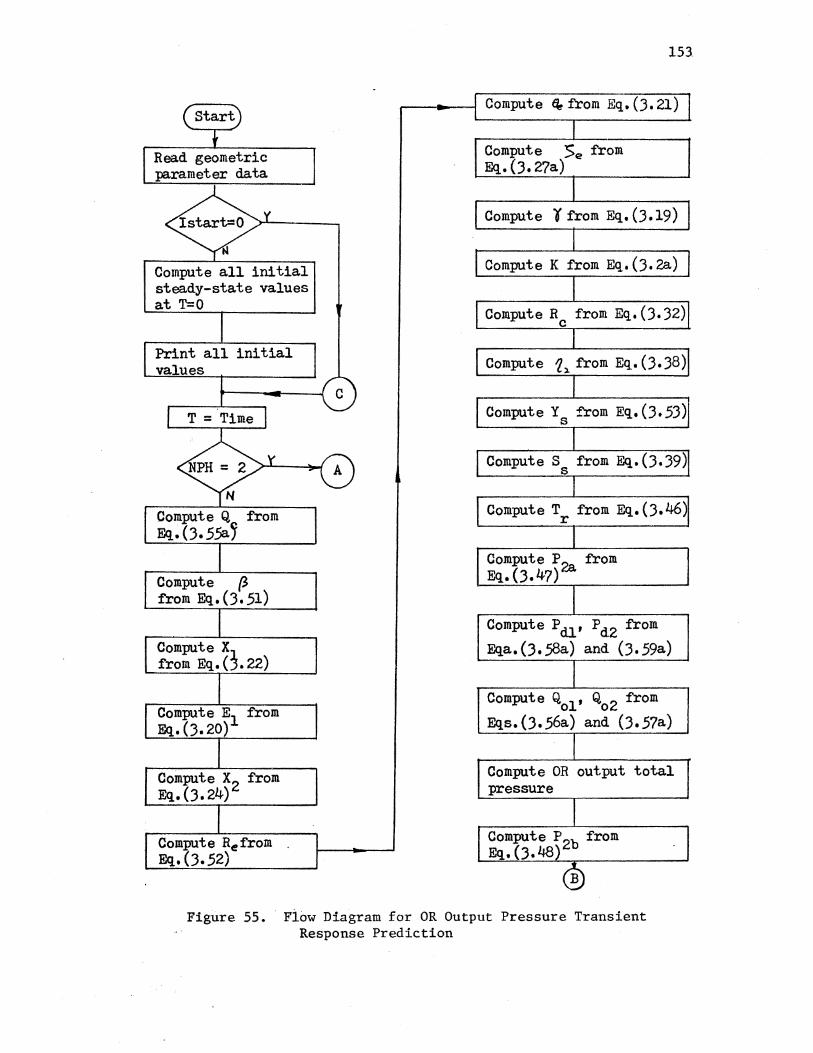
Compute all initial steady-state values at T=O
Print all initial values
N
Compute Q from Eq.(3.5.5a~
Compute (3 from Eq. (3. 51)
Compute X from Eq. (3. 22)
Compute E1 from Eq. (3. 20)
Compute x2 from Eq.(3.24)
Compute Re from . Eq. (3.52)
153
,----ti--l Compute ~from Eq. (3. 21)
Compute .Se from Eq.(3.27a)
Compute o from Eq. (3.19)
Compute K from Eq.(3.2a)
ComputeR from Eq.(3.32) c
Compute 'l'l. from Eq. (3.38)
Compute Ys from Eq.(3.53)
ComputeS from Eq.(3.39) s
Compute T from Eq. (3.46) r
Compute P 2a from Eq.(3.47)
Compute P dl, P d2 from
Eqa.(3.58a) and (3.59a)
Compute Q01 , Q02 from
Eqs.{3.56a) and (3.57a)
Compute OR output total pressure
Compute P2b from Eq.(3.48
Figure 55. · Flow Diagram for OR Output Pressure Transient Response Prediction

Compute P1 from Eq.(J.50)
Compute X from Eq.(J.Jl) r
N
Compute A from Eq.(J.43) v
Compute V from Eq.(J.42)
Compute 8e from Eq. (J. 54 by implicit iteration
ComputeR from Eq.().21) . e
Compute x2 from Eq.(J.23)
Compute X from Eq.().24 e
Compute A from Eq.(J.l5) c
Compute Cdc from Eq.(B.4)
154
Print switching time
Compute all steady-state values by iterations for a given Pct(T)
Compute~ from Eq.(J.55a) c
Compute ~ from Eq. (3. 73)
Compute X1 from Eq.(J.79)
Compute E1 from Eq.(J.77)
Compute X2 from Eq.(3.24)
ComputeR from Eq.(J.81) e
Compute 6e from Eq. (J. 78)
Compute ~e from Eq.(J.27a
Compute t from Eq. (3. 76)
Compute K from Eq.(J.2a)
ComputeR from Eq.(J.82) c
Figure 55. (Continued)

Compute Y from Eq.(3.84) s
ComputeS from Eq.(3.83) s
ComputeT from Eq.(3.46) r
Compute P2a from Eq.(3.69)
Compute Pdl' Pd2 from Eqs.(3.86) and (3.87)
Compute Q01 , Q02 from
Eqs.(3.56a) and (3.57a)
Compute OR output total pressure
Compute P2b from Eq.(3.70)
Compute P1 from Eq.(3.72)
Compute Xr from Eq.(3.41)
N
y
Compute A from Eq.(3.67)
Compute V from Eq.(3.64)
Compute Be from Eq. (3.85) by implicit iteration
ComputeR from Eq.(3.78) e
Compute x2 from Eq.(3.80)
!Compute Xe from Eq.(J.24)
Compute Ab from Eq.(3.66)
Compute~ from Eq.(3.65)
Print all final values
Plot desired variables
Figure 55. (Continued)
155
156
Values of the unattached-side pressures (P2a and P2b) may be deter-
mined by iterations at each lime step. Since these iterations at every
time step require excessive computer time, the following alternative
method was chosen. For example, the pressure P2a may be computed as
follows:
Step 1. Compute Qb from Equation (3.47a) based on the value of
p2a(t- ~t).
2. Compute ~ from Equation (3.47b) based on the values of
P2a(t- ~t) and P2b(t- ~t).
3. ComputeS from Equation (3.47d). w
4. Compute Qe3 from Equation (3.47c).
5. Compute the net flow rate into region 2a from
6. Compute a differential pressure EP2a from
~p = EQIEQI 2a (B + A )2
b w
7. Compute a new P2a from
C.2 Selected Computer Program Listings
The following computer programs are listed in this section:
1. Computer program 2 which was used for the computation of the
steady-state jet reattachment distance;
2. Computer program 2 which was used for computations of the switch-
ing time and the OR output total pressure transient response; and
3. Computer program 3 which was used for the computation of the
return time.
157 .
Since these computer programs were primarily written to calculate
predicted values to be con1pared with experimental data, they are only
cursorily documented. User-oriented programs could be evolved from these
programs. The definitions of variables and parameters used in the pro
grams are presented in Table III.

158
TABLE III
DEFINITIONS JF VARIABLES AND PARAMETERS
p (1) = a P(Sl) c: 1T X(27) = p X(62) = n 1 cb 2 p (2) = a
2 P(52) = 180/1T X(28) = p X(65) = w c ol
p (3) = D 1 P(53) = c X(29) = p X(66) tc = w o2 p (4) = D
2 = 67/90 X(33) = n 1 X(67) = c de
p (5) = D P(58) = cos al X(34) = P2a(phase II) X(69) = Re 3 c p (6) = B P(59) = sin a1 X(35) = e X(70) = Re' c p c p (7) = B b P(60) = cos a2 X(36) = P2a(phase I) X(74) = cos B
p (8) = B vl P(61) = sin a2 = Pb(phase II) X(75) = sin B p (9) = D P(62) = s X(37) = R X(76) = e /c s 0 es e P(lO) =X X (1) =X X(38) = Z X(77) = A. vl e w P(ll) = L X (2) = X X(39) = ~ y (1) = Q c r c P(l3) = L X (3) = s X(40) = s y (2) = v ol e p P(l4) = L X (4) = R X(41) = T y (3) = Qol o2 e p P(l5) = L X (5) = R X(42) = y y (4) = Qo2 th c p P(l6) = b X (6) = y X(43) = Qe3 s s P(l7) =AR X (8) = e X(44) = ~ e P(l8) = 0 X (9) = y X(45) = Qe4 P(l9) = v X(lO) = 13 X(46) = S
w P(20) = p X(ll) = T X(47) = 11 r w P(22) = q X(l2) = T X(50) = x1 s s P(23) = u X(l3) =A X(51) =X s c 2 P(24) = Re X(l4) =A X(52) = K s v P(26) = t t X(l5) =~ X(53) = E 1 P(31) = I' X(l6) = Qe2 X(54) = E c 2 P(33) = I' X(l8) = Qb X(55) = y ol r P(34) = I' X(20) = P02 X(57) = s o2 s P(36) =X X(21) = P1 X(58) = s v2 v P(41) = Final value X(22) = P2b X(59) = 11
of P v tc X(23) = pdl X(60) = G
P(42) = T ri X(24) = pd2 X(61) = z;

c C CO~PUTER PROGP.~~ 1 - CO~PUTA110N OF THE C SIEA~Y-STATE JET REATTACHKENT DISTANCE c;
c
Oll':fliSION 00 ICO 11=1,100 PCI!>=O.O
100 XC Ill=O.O DO 200 11=1,5
200 Y(l;)=O.O P(l}=l~.
1'(2)=15. P(3)=0.5 P(~)=P(3)
1'(5)=0.0 1'(6)=1.0 P(7l=l.O P( 61=2.2 P<9)=2:.o I'Cl0l=13.G35 ?C! 1)= .... ~ P(!2l=~.o P<J 3)=30.0 F(lq=30. PC15):3.2 P(l6}=l.O PCi1)=I.O POEl=lO.S P< !<:)=l.25I7E-2 P(2C)=l.l23:'-7 P~S:1=:.E-S
PC51):3.1~!5~?G54 FC~2)=l<G./P(51)
P<S3>=<>7.n~.
p ( 5" > = 6 7 ;, p ( 52) P(SL>=•(l)/v(52) P(;7)=r(2)/P(52) P(~ol=C~S{P(~6))
p c ~ s ; = ~ i ~o: ( p { c.~))
f(!.":;=~~~(P(~7))
PC~!; o S l ~ ( f' (:, 7}) PU.;')=?C 1 q)/3. P{e3J=l.,,csz>
CI(7),P(l00),X(100),Y(5)
P(6~)=(l.+l./P(17ll*•2 X(6~)=(P(3)•P(5)+0.S)•P(58)•P(9)0P(59)
X(66)=(P(~)-?(5)+0.5)0P(60)+P(9)~P(61)
\i~l!f(!.~lLCO)
12CC rC.i "!H "I•> ~-lTf(6,!300) P(3l
130~ F:••;T(3X,.Dl=",F7.~)·
HI )~~.0 C': 3C~ JJ=l ,7 l(IQ)=A1:N(Y(l)•Y(l)/P(6))
10 X(~3)=X(l~)
c
1(7~)=CC~(XC10))
XC7S)=S;~(X(l0))
X~Sc)=:.S•(P(6)+X(75)) /P(58) X(53l=P(3J+X(~0)•PC?9)+Q.So(J.O-X(7~))
C l1ER~T10NS FOR X{8) c
lC\JI<T=O
159
c
P(55}=0.05 X(B) =(P(56}tP(54))/3.0 X(76)=X(8)/P(53) X(62)=P(S3)t1AN(X(76)) X(6l}=ATAN(X(82)) X(9)=X(6l)+X(8)-X(l0)-P(56) X(ll)=2.0~COS((P(5l)tX(9))/3.)
X(81)=((2.•Y(l)tl.)/X(ll))*•2 X(3)=P(62l•(X(81)-J.) X(52)=X(3)/(0.62*X(76)+0.3B•SIN(X(76})) X(4)=X(52)tSl~(X(76))
X(8~)=X(4l*SlN(X(8)-X(l0)-P(56))/P(58} P(66)=X(8~)-X(53)
lF(ABS(P(66)).LT.I.E-~~X(53)) GO TO 26 20 KOUNT=KOUNT+l
lf(KCUNT.GT.IOO) GO TO ~6
X{8)=X(B)+P(55) X(76)=X(8)/P(53) XCS2)=P(53)tTA~(X(76))
X(6l)=ATAS(X(82)) X(9)=X(6l}+X(S)-X(l0)-P(56) X(ll)=2.C•COS((P(5J)+X(9))/3.) X(81)=((2.•Y(l)+l.)/X(ll))*•2 X(3)=P(62)*(X(81)-l.) X(52)=X(3)/(0.62tX(76)t0.386SJN(X(76))) X(~)=X(52)$SJN(X(76)) X(84)=X(4l•SJN(X(S)-X(l0)-P(56})/P(58) P(67)=X(84)-X(53) IF{A~S(P(67)).LT.l.E-4•X(53)) GO TO 26 lf(lP(6~)•P{67).GT.O.O).ASJ.(ABS(P(67)).LT.ABS(P(66)))) GO TO 22 IF({P(66l•P(67).GT.O.O).A~3.(A8S(P(67)).GT.~BS{?(66)))) &0 TO 2~ IF (P(66)•PC67).LT.O.O) ~0 TO 25
22 P(66):P(67) GO TO 20 ·
2~ P(66)=P(67) P(55)=-P(55) GO TO 20
25 P(66)=P(67) P(55)=-0.l•PC55) GO TO 20
C ENO OF ITERATIONS FOR X(8) c
26 XC51)=X(4)•COS(X(8)-X(l0))/P(5S) X(l)=X(50)+X(51)
c C XR t
c
X(80)=X(3)+P(62) X{63)=SORT(P(62)/X(80)) X(Sl)=O.S•X(80)/P(l8) X(82)=((l.+X(ll))J(l.-X(ll)))•((l.-X(63))/(l.+X{63))) X(2)=X(l) -X(8l)#ALOG(X(S2))/SIN(X(9))
C RCL c
X(37)=Q.SoX(52)/P(53) X(80)=X(37)+0.5 XC8l)=P(9)-0.S~P(6)-X(80)•X(75) XC82)=X(BO)~X(7~)+P(5)
X(~3)=ATAN(X(81)/X(82))
X(35)=Q.So(X(l0)+X(33)) X(~0)=2.cX(37)oY.(35)
X(8l)=X{40)+P(62) X(~l)=~ORT(P{62)/~(81))
X(~2)=(.5oX(81)/P(l3))~AlOG((l.+X(~l))/(l.-X(~l)))
160

c
X(82)=0.5-X(42) X(83)=COS(2.~X(35))-l.O
X(5)=X(37)+.5•(1.+X(82)•(2.•X{37)+X(82))/(X{37)•XC83)-X(82)))
C ETA2,SS c
c c t
t c. c.
t t c
t c c
35 36
X{81)=P(9)-0.5•P{6)-X{5)•X{75) X(82)=X(5)•X(7~)+P(5) X(62)=ATA~(X(81)/X(82))
X(57)=X(5)•(X(l0)+X(62))
P2 , Pl
XC16)=0.0 1(22)=0.0 X{2l)=X(22)-2.0/X{5)
PCB
X(27)=(X(2l)+X{22))12.
AC
X(!3)=0.5•P(6)•X(75)+(P(3)+0.5+P{6)~TAN(P(S6)))*X{7~)-0.5 lf{X(l3}-?(6)) 36,35,35 X<l3)=P(6) C'J~TaUE .X(l8)=0.0
BT
X(2B)=XC27)+ (l{l)/X(l3))••2 l{El)=Y(l)~Y(l)/P(6)
xc e 3)= o. s.•c xu B>-x<z 2 > >• PC 6 > X~lC)=~1A~(X(83)+X(Bl))
XC!O)=XC4a)-X(l0) IF (!5S(X(oG)).lT.l.E-~) GO TO 50 GO T::J 1 ()
'>6 li~ITH6, 1002} 1002 fCR~AT("G",3X, •• ARNTNG 3 = ITERATIONS FOR X{8) 00 NOT CONVERSE") 50 WRITEC6,2200) Y{l),X(2),X(l0),KOUNT 2200 F~R~AT("O", 3X,2Fl2.6,El6.6,3X,l3) 70 T(l)=T(1)+0.05 300 CONT HWE
STOP END
161
c C COMPUTER P~OGRAR 2 - COXPUTAT10NS OF THE S~ITCHJNG TIME C A~O THE OR OUTPUT TOTAl PRESSURE TRANSIENT RESPONSE t
DIMfNSIDK F(l01),l(10l),C1(7) IF (1ST!RT.E0.0) GO TO SO !iPH=l 102=0 !C3=0 DD 5CO !1=1,1 00
50!1 X(Il)=O.O
t
PC51)=3.!4!59265~
P(52)=le0./P(51) 1'(53)=67./SO. P(5~)=67./P(52)
PC56)=P(l)/P(52) P(57)=P(Z)/P(52) PC58)=C~S(P(56))
PC59)=SIH(P(56)) PC6C)=COSCP(57)) P(6l)=Sl~(PC57))
P(62l=P(lS)I3. P(63)=1./P(52) PC65)=(1.•1./P(17l)••2 X(65)=(P(3)•P(5)•0.5)•P(58)+P(9)•P(59) X(66}=(P(4)-P(5)+0.5)•P(60)+P(9)~P(6l)
C COEFf fJP. C~ Cl(l)= 6.9056~5E-2 C1C2)= 2.067S~CE-l (1(3)= 2.~~412,~-1
CIC~>=-5.~:~3>9E-2
CIC5)=-7.J3939GE-2 CI<6>= 4.e3~4S~F-2 Cl(7)=-8.~77535E-3
c c
c
PC26)=P(l6)/P(23) PC42}=2.5r-3/PC26)
T(l):o0-0 X(l 0)=0. DO 410 I=I ,10 X(H)=COSOOQ)) XC75>=SI~(X(l0))
X(50)=C.5•(P(6)+X(75)) /P(58) X(53)=P(3)~X(50)~PC59)*C.5~(1.0-X(74))
t ITER~TIDNS FGR X(8)
KCU"''T=O PC55)=0.05 X(B) =(P(56)+P{5~))13.0 X(76)=X{c)/P(53) X(8Z)=PCS3J•TIN(X{76)} l(6l)=ITtN(X(£2)) l(9)~X(6l)+J(2)-X{l0)-P(56)
XCll)=2.0•COS((P(51)+X(9))/3.) X(81)~((2.0T(l)+l.)/X(ll))~•2
X(3)~P(62)#(X(8l)-l.)
X(52)=X(3)/{0.62~X(76)+0.38*SIN(X(76))) l(4)=X(52)•SINCX(76)) X(S4)=X(4)•$I~(X(B)-X(l0)-P(56))/P(53)
162

P(66)=X(84)-X(53) IFCABS(P(66)).LT.l.f-4*XC53)) GO TO ~26
~20 KOUNT=KOUNTtl IFCKOUNT.GT.!OO) GO TO ~~6 X(8}=X(8)•P(55} X(76}=X(8)/P(53) X{82)=P(53)oTAN(X(76)) X(61)=ATAN(X(82)) X(9)=X(61)•X(8)-X(10)-P(56) X(ll)=2.0•COS((P(5!)+X(9})/3.) X(81)=((2.oY(l)+!.)/X(ll))**2 X(3)=PC62)o(X(81)-l.) X(52)=X(3)/(0.62*X(76)+0.3S•SIN(X(76))) X(4)=XC52)•SIN(X(76)) X(8~)=X(4)•SIN(X(8)-X(l0)-P(56))/P(58) P(67)=X(8·)-X(53) IF(ABS(P(67)).Ll.I.f-~*X(53)) GO TO ~26 lF((PC66)oP(67).GT.Q.O).AND.<ABSCP(67)).lT.ABS(P(66)))) GO TO 422 IF((P(66)0P(67).GT.O.O).AND.(ABSCP(67)).GT.ABS(P(66}))) GO TO ~24 IF (PC66)oP(67).LT.O.O) GO TO 425
~22 P(66)=P(67) GO TO 420
•24 P(66)=PC67) P(55)=-P(55) GO TO 420
•25 P{66)=P(67)
c
P(55)=-0.l*P(55) GO TO 420
C END OF ITERAT!ONS FOR X(S) c ~26 X(5l)=X(4)$(0SCXiSJ-X(!C)}/P(58)
X(l)=X(50)•X(51) c C XR c
t
X(80)=X(3)+P{62) X{63)=SORT(P(62)/X(80)) X(81}=0.5oX(80)/P(l8) X(82)=((1.+X(!l))/(l.-X(ll)))•({l.-X(b3))/(l.•X(63))) X(2)=X(l) -X(Bl)•ALOG(X(82))/SIN(X(9))
C RCL c
t
X(37)=0.5•XC52)/P(53) XCBO)=X(37)+0.5 X(Bl)=P(9)-0.S•P(6)-X(80)•X(75) X(82)=X(BJ);X(7~)•PC5)
X(33)=ATAN(X(Sl)/X(82)) X(35)=C.5~(X(l0)+X(33))
XC~0)=2.~X(37)#X(35)
X(Sl)=X(~O)+P(62) X{~l)=S0Rl{P(62)/X(81))
X(~2):(.5;X(8!)/P(l8))~Al0G((l.+X(4l))/(l.-X(~l)))
X(82)=0.5-X(42) X(83)=COS(2.•X(35))-l.O X(5)=X(37)+.~*(l.+X(82)*(2.•X(37)+X(82))/(X(37)=XC83)-X(82)))
C ETA2 • SS c
c
X(8l)=P(9)-0.5oP(6)-X(5)•X(75) X(82)=X(5)*X(7~)+P(5) X(62)=ATAN(X(8l)/X(82)) X(57)=X(5)~(X(l0J+X(b2))
C QE2
163
c X(16)=0.S•CSORT(l.+X(57)/P(62))-l.)
c C PI c
c
X(82)= P{7)+P{8)+X(66) X(22)= -(X(16)/X(B2))**2 X(2l)=X(22)-2.0/X(5)
( PCB c
l(27)=(X(2l)+l(22))/2. c C AC c
XC13)=0.5~P(6)•XC75)+(P(3)+0.5+P(6)•TAN(P(56)))$X(7~)-0.S
1F(X(13)-P(6))436,435 1 435 435 X(13)=P(6) 436 (OJ.TINUE (
c Q!! c
c c c
"10 c
' c 1,45
' c
'
H6 1002
50
'
51 101
.l(18}=
l(Z£)=X(27) X(o3)=G.5•(X(2B)-X(22))•P(6) X(!0)=~l~~(X{83))
CD~T!HUE
OC20 0)
T{~)=-X{66)tSORT{-X(22))
XC12)=-1.0 l(23)=.25*(3.oX(ll)-X(ll)**3-3.•X(12)+X(12)•*3)/X(65) 7.(3l)=X(23) Y(3)=X(65)*SORT(X(31))
V(TO)
l(66)=0.25*?(53)*X(52)*X(52)•(X(76) - 0.5•SIN(2.•X(76))) X(87)=.5~X(53)~X(4)•COS(X(8)-X(l0)) X(58)=C.5•X(5C)t(P(3)+X(53))*P(58) Y{2)=X(96)+X(€7)+X(88) X(~6)=X(22)
X(67)=C.O! f(o\6)=1{22)
YC l)=~.C t;O TC 50 w;>.IHC6,1002) FG~~AT{"C",3X,"~A~NlhG 3 = ITERATIONS FOR XCS) 00 NOT CONVERGE'} &0 TO (51,200), "Ph X(29}=(P(41)-P(~6))#(l~-EXPC-TIHE/P(42)))+P(~6) 0Y(l)=X(67)0(X(2S)-X(28)-Y(l)*ABS(Y{l))/(X(o7)•P(6))~$2)/P{31)
lF(T(l).LT.:.Ol J(l)=O.O f:T XC28}=X(27)+ (Y(l)/X~l3))**2
X(8ll=Y(l)•Y(l)/P(6) X{83)=C.S*(X(28)-X{36)}*P{6) XC10)=A7A~(XC€3)+X(Bl))
X(H)=COSCXC 10)) X(75)=SIN(X(lC)} X(50)=C.5•(P(6)+X(75)) /P(58) XC53)=P(3)+X(5~)~P(59)+0.5*(1.0-X(7~)) :X{5l )=X(l)-X( 50)
164
XC81)=(X(51)•PC59)+X(53))**2+CX(5l)#P(58))••2 X(~)=SQRT(X(81))
XC81)=XC53)•PC58)/X(~)
X(8)=ARSIN(X(81))+X(10)+P(56) X{76)=X(8)/P(53) X(82)=P(53)•TAN(X(76)) X(61)=ATAN(X(S2)) X(9)=X(61)+X(8)-X(10)-P(56)
t RCl X(S2)=X(~)/SJN(X(76))
X(37)=0.5•XC52)/P(53) XCBO)=X(37)+0.5 X(81)=P(9)-0.5~P(6)-X(80)•XC75) X(82)=X(80)*X(7~)+P(5)
X(33)=ATt~(X(81)/X(82)) X(35)=0.5•(X(l0)+X(33))
C SP X(40)=2.tX(37)*X(35)
t yp X(Sl)=X(40)+PC62) X(~1)=SQRT(P(62)/X(81))
X(42)=(.5oX(81)/P(18))~ALOG((I.+X(~l))/(l.-X{~l)))
X(82)=0.5-X(~2)
X(S3)=COS(2.~X(35))-l.O X(5)=X(37)+.5•(l.+X(S2)t(2.tX(37)+X(82))/{X(37)•XC83)-X(82)))
t ETA2 X(8l)=P(9)-C.S•PC6)-X(5)tX(75) X(82)=X(5)~X(7~)+P(5)
X(62)=AlAN(X(81)/X(82)) t YS
XC83)=X(8l)•t2+X(82)~•2
X(60)=S0Rl(X(63)) XC6)=X(5)-X(60)
c ss XC57)=XCS)•(X(l0)+XC62))
t TS X(80)=P(l8)*X(6)/(X(57)+?(62)) X(8l)=EXP(X(80)) ~(82)=EXP(-X(S0)) XC12)=(X(81)-X(S2})/(X(8l)+X(S2))
C SPLITTER EFFECT X(77)=(1.-l.S•X(l2)+.5•X(12)**3)•COS(X(9))+l.+I.5•X(l2)-
1 o.s~x<I2>•~3 XC7S)=~RCOS(X(77)12.)
X(l1)=2.0*COS((P(5l)+X(78))13.) C PBE
XCIS)= P(7)•SCRT(-X(36)) lF(X(10)) 164,164,102
102 X(82)=X(5)~X{75)+.5tP(6)
X(83)=P(36)•PC60) IF(X{82)-X(83)) 172,172,173
172 X(~6)=X(5)tX(10)
X(~7)=1.62S•(X(~6)+P(62))/P(l8)
XC38)=X(82)0TAN(P(57))+P(4)+.5-X(5)*(1.-X(7~))-X(~7) ~0 TO 17~
173 X(~7}=l.B25~(X(46)+P(62))/P(l8) X{38)=P(36)•PC6l)+P(4)+.5-(X(6)+P(5))-X(47)
174 JF(X(38)) 103,103,10~ 103 XC38)=0.0
X(~~)=O.O
GO TO 163 10~ X(BC)=X(22)-X(36)
JF(X{90)) 162,161,161 161 X(~4)=X(38)oSORT(X(80))
GO TO 163 162 X(4~}=-X(38)•SORT(-X(80))
165

c
163 X(~3)=0.5•CSORT(l.+X(46)/P(62))-l.)
xce3>=xcta>•xc~~>-xc.r.3) X(B4)= P(7)+X(38) X(36)=X(36)+X(83)*ABSCX(83))/X(84)••2 IF(1(36).GE.O.O) X(36)=0.0 GO TO 165
164 XC46l=O.O X(47)=0.S XC36 )=X( 22) X(H)=-~(18)
XC43)=0.1l X( 3B)=P(7)
C PD2 c 002
c
c
c.
c.
165 XC23)=.25o(3.•X(ll)-X{11)~t3-3.tX(12)+X(!2)••3)/X{6S) X(31)=X(23) 0T(3)=(X(31)-X(26)-T(3)tAB5(Y(3))/XC55)tt2)/P(33) X(2~)=.2~•C2.+3.*X(12)-X(12)*>3)/X(66)
XC32)=X(22)+X(24)
175
176 177
107
166
167 168
108
169
170 !11
109
lF(X(57)-X(46)) 175,176,176 XC22)=X('o6) GC TO 117 XC E 2 )=X( 57) X(45)=0.S~CSCRT(1.+X(S2)/P(62))-l.)-X(43)
0T(4)=(X(32)-X(26)-T(4)tAeS(Y(4))/X(66)>~2)/P(34) IF(T(~)) 107,1~8,108
XCB2)=P(8)•5C-T(-X(22))-T(4)-X(44)-X(4S) iF{X{44}) 166,167,167 X(e3)=F(B)+X(66)+X(38) C.G TU 16 6 X(d3)=P(8)+X(66) X(17)=X(32)=A3S(X(82))/X(83)~*2
GO 10 109 X(62)=FC2)*SORT(-X(22)}-X(44)-X{~5) Jf(~(4~)) 169,170,170 . XCE3):P(8)+X(3S) GO TO 171 X(S3)=P(8) XC17)=XCE2)*ABSCXC82))/X(83)**2 POUT X(2C)=(T(4)/X(o6))t*2 X(22)=XC22)+X(17) lf(J(22).&f.O.O) X(22)=0.0 P1 X(81)=XC46)/X(57) X{21)=X(e1)*X(36)+(1.-X(8l})~X(22)-2./X(5)
PCS 1(27)~{~(21)+;(36))/2.
X~
X(3)=7(52)~(0.62~~(76)+0.3BtSIN(X(76))) X(60)=X(~)+P(62)
X(63)=S~RT(PC62)/1(80))
X(81)=0.5•X(8Q)/P(l8) XC82)=((l.•X(1!))/(l.-X(11)))*({1.-X(63))/(1.+X(63))) X(2}=XC1) -X(8l)•ALDu{I(82))/SIN(X(9))
C OV/!JT IF(X(2)-P(I0)) 110,110,111
110 0T(2)=T(1)+0.5•(1.0-X(l1)/X(63)) l(H)=O.O X(19i=C.O GO TO 120
111 IF<I02.EC.l) GO TO 116 XCEI)=P(lQ)oP(S8)-X(5)•X(75)-0.S•PC6) X(82)=X(5)•XC7~)-P{1C)~P(59)-(P(3)+C.5) X(39)=~TA~(X(81}/X(82))
166
c c c
c c c
112
113
114 115 116
120
121
122
123 12~
125
130 132 1100 135
139 140
c
136 137
c
lf(X(39)-P(56)) 112,112,113 102=1 GO TO 115 X(58)=X(5)o(X(l0)+X(39)) X(59)=1.8Z5t(X(58)+P(62))/P(18) X(I~)=X(5)-X(59)-X(81)/SIN(X(39))
lf(X(14)) 110,110,11~ lf(X(l~)-P(8)) 116,115 1 115 X(l4)=P(8) X(19)=X(14)~SORT(-X(21))
0Y(2)~Y(1)+0.5*(1.-X(11)/X(63))+X(19)
I~PliCIT FN FOR THE
F(l )=X(8) l{2)=X(8) X(85)=X(l) X(88)=0.S*X(50)•(P(3)+X(53))*P(58) 00 130 N=2,30 1=0 X(S)=A8~(Z(I.;))
lf(X{8).Gf.P(54)) X(8)=P(54)-P(63) ]F(X(8).LE.O.O) X(8)=P(63) X(76)=X{8)/P(53) X(4)=X(53)*P(58)/SIS(A3S(X(8)-X(l0)-P(56))) X(52)=X(4)/SIN(X(76)) X(87)=.5*X(53)~X(4)*COS(ASSCX(8)-X(10)))
X(81)=4.t(Y(2)-X(87)-X(88))/(X(52)~X(52))+.50P(53)*SIN(2.*X(76))
f(N+l)=ABS(X(Sl)) IF(N.Gl.Z) GO 10 123 lf(l) 123,122,123 Z(N-l)=F(N-1) l(N)=F(N+l) f(N)=F(N+l) 1=1+1 -IFCI.GT.20) GO TO 132 GO TO 121 lf(Z(N)-Z(N-1)) 125,12~,125 l(N+1 )=l(N) GO TO 135 P(68)=(F(N+l)-F(N))/(Z(N)-Z(N-1)) IF(P(68).f0.1.) GO TO 122 PC69)=PC68)/(P(68)-1.) l(N+l)=P(b9)*Z(N)+(l.-P(69))*f(N+1) f(70)=AB~(Z(N+1)-Z(N))
lf(P(70).LE.l.E-6) GO TO 135 co:o~Tl ~~ue
liR llE<6,11 00) FOR~AT<·o·,3x,·~ARNING 4= I~PLICIT FN FOR X(8) ODES NOT CJNVERSE') X(B)=ICN+l)
END OF IKPLICIT FN FOR THE
IFC(X(B).LE.(X(10)+PC56))).0R.(X(8).GE.P(5~))) GO TO 139 X(~)=X(53}oP(5S)/SlN(ABSCX(8)-X(10)-P(56)))
X(5l)=X(4)~COS(X(S)-X(10))/P(58)
X{l)=X(50)+X(51) GO TO HO XO )=X(B5) COIHINUE AC XC13)=0.S•P(6)*X(75)+{P(3)+0.5+P(6)•TAN(P(56)))oX(7~)-0.5 lf(X(13)-P(6)) 137.136,136 X(l3)=P(6) COl'. TINUE coc
167

lF(T(l).fO.O.O) GO TO 1~7
X(69)=T(l)oP(2~)
X(70)=X(69)/((P(l1)+1.)oP(65)) X(8G)=ALCG1C(X(70)) X(b7)=CI<l) DO Hb J=1,6
146 X{67)=X(67)•CICJ+l)tX(80)*tJ lF()(67).lE.O.O) 1(67)=0.01
c 08 147 C:JNTHi\Jt
c C SIIITCHI>IG
IFC103.f0.1) GO TO 155 IFCX(6).L£.(P(~)-P(3))) GO TO 295 X(7)=0.95tX(66)cSQRT(X(79)) IC3= l
155 JF(Y(4).lT.X(7)) GO TO 300 NPH=2 E~DTI~=TIME+70C.O
II~Ilf(b,160)PC4!),TIME,YC!),Y(4),X(7),X(6),X(20) 16C f0R~Al{"0",3X,F16.5,F16.3,1PSE16.6)
c c
SHE1=P(l) P( l)=PC2) P(2)=SHEl SHt2=PC3) P(3)=~( ~)
PCO=St>:O? St'IE3=PC6) P<6)=P(7) PO)=SAVE 3 Sl.\'F4=P(l0) PC10l=PC36) PC 36)=SAVE~ P(5)=-PC5) Sl.HS=I"C 11) P(ll)=P(ll} PCl2)=SA"VES X{68)=X(67) X{67)=0.0 P{50)=1.E-3
C lTfRAR~TIONS FOR OBCTO) IICR=O
c
llER=O 105=0 X00=0.2 ll(&S)=X{lll) X(2!)=l(l)tl(l)/P(7) X(Z2)=X(lc)oX(l6)/P(6) X(!C)= ~l!.(X(82)-X(81))
10 ITE~=Ilf~+1
IFCITF~.&T.20) NCR=2 X(7~)=CGS(X(l0))
X(75)=~I~(T.(lC))
X(SC)=0.5>(P(6)+~C75)} /P(58) XC53)=f(3)+~(~0)oPC59)+Q.5o(l.O-X(7~))
C ITE~ATIONS FOR X(8) c
IF(X(lO).GT.-0.35) GO TO 11 105=1 X(6)=C.06 GO TO 12
11 I.OUNT=u PC55)=0.02
168
X(8) =0.1 12 X(76)=X(8)/P(53)
XC82)=P(S3>•TAN(X(76)) X(6l)=Al~N(X(82)}
X(9)=X(6l)•X(8)-X(l0)-P(56) X(ll)=2.0•COS((P(5I)+X(9)}/3.) X(81)=((2.oX(l8)+1.)/X(ll))tt2 X(3)=P(62)t(X(81)-l.) X(52)=X(3)/(0.62tX(76)•0.38oSINCX(l6))) X(4)=X(52)•SIN(X(76}) X(84)=X(4)0SIN(X(8)-X(I0}-P(56))/P(58) IF(IDS.EO.l) GO TO 26 P(66)=X(84)-X(53) IF(A8S(P(66)).LT.l.E-4•XC53)) GO TO 26
20 KOUNT=KOUNT•l IFCKOU~T.GT.!OO) GO TO 46 X(8)=X(S)•PC55) V~=P(63}/3.0
IF(X(S).Lf.Q.O) X(S)=VK X(76)=X(8)/P(53) X(82)=P(53)oTtN{X(76)) X(6l)=ATAN(X(82)) X(9)=X(6l)•X(8)-X(l0}-P(56) X(ll)=2.CoCOS((P(5l)•X(9})/3.) X(81)=((2.•X(l8)+1.)/X(ll))oo2 X(3)=P(62)•(X(81)-l.) X(52)=X(3)/(0.62tX(76)•0.38tSIN(X(76))) X(4)=X(52)oSIN(X(76)) X(84)=X(4)•SIN(X(8)-X(l0)-P(56))/P(59) P(67)=X(84)-X(53) JF(A8S(P(67)).LT.l.£-40X(53)) GO TO 26 JF((P(66)oP(6l).GT.O.O).A~O.(ABS(P(67)).l!.ABS(P(66)))) GO TO 22 lF((P(66)oP(67).GT.O.O).AND.(ABSCP(67)).GT.ABS(P(66)))) GO TO 24 IF (P(66)*P(67).LT.O.Ol GO T~ 25
22 P(66)=PC67) GO TO 20
2~ P(66)=PC67) P(55)=-P(55) CO TO 20
25 P(66)=PC67)
c c
46 1002
c
c c c
c
26
P(55)=-0.l~P(55)
GO TO 20
END OF ITERATIONS FOR X(8) WRITE(6 0 1002) FORMA1('0" 0 3X 0 "WARNING 3 = ITERATIOSS FOR XC8) 00 NOT CONVERSE")
X(Sl)=X(4)~COS(X(8)-X(l0))/P(58)
X(l)=X(50)+X(51)
XR
X(80)=X(3)•PC62) XC63)=SORT(P(62)/X(80)) xcsJ>=c.~•xcso>tPCIB> X(82)=((l.+X(ll))/(l.-X(ll)))o((l.-X(63))/(l.+X(63))) X(2)=X(l) -X(6l)~ALOG(X(82))/SIN(X(9))
C RCL c
X(37)=0.5oX(52)/P(53) X(80)=X(37)+0.5 X(8l)=P(9)-0.5oP(6)-X(8Q)oX(75) X(82)=X(80)tX(74}-P(5) XC33)=ATAN(X(Sl}/X(82)) X(35)=0.5c(X(l0)+X(33))
169

X(40)=2.eX(37)tX(35) X(8l)=X(~O)+P(62)
X(4l)=SCRT(P(62)/X(81)) XC42)=(.SoX(81)/P(l8))oALOG((l.+X(41))/(l.-X(41))) X(€2)=C.5-X(42) X(S3)=(0S(2.•X(35))-l.O XC5)=X(37)+.5t(l.+X(82)*(2.*X(37)+X(82))/(X(37)tX(83)-X(82))) lf((X(5)-X(37))-20.0) 17,15,15
15 X(5)=X(80) c; C ET A2 , SS c;
t
17 X{8l)=P(9)-0.5tP(6)-X(5)tX(75) XC82)=P(e)+X(65) J(62)=~T~~(X(8l)/X(82)) X(57)=X(5)t(X(l0)+XC62))
C OE2 (
X(16)=0.5t(SQRT(l.+X(57)/P(62))-1.) ( ( PI c.
t
X{23)=J(l~)-T(l) !F(XCB3).lE.O.G) X(83)=0.0 X(6Z)=P(8)+P(29)•X(66) X(22)= -(X(83)/X(82))•*2 X(21)=X(22)-2.0/X(5) IF(J(?l).Gf.O.O) XC21)=-0.02
( l!s C C9 t
l!H=O X(15}= 0.5tP(6}tX(75)+(P{3)+.5+P(6)•TAN(P(56)))*X(74)-.5 lf(X{l5)-P(6)) 31,30,30
30 X(15)=P(6) -X(1e)= P(6)tSQRT(-X(21)) X(36)=X(21) 104=1 GO TC 32
31 XCia>=X(l5)*SORT(-X(21)) X(36)=-(X(l8)/P(6))~•2
IFCXCl~).GE.C.SO #P{c)) 104=1 32 C ') '<T I'IUE
IF(t8~(~(18)-X(£~)).LE.P(50)) NCR=l c; liT
X(BI)=Y(l)*Y(l)/P(7) XC22)=1(22)•(l(l)/X(l3))**Z IFCID~.f~-1) GO TO 33 X(82)=X(l8)oX(l8)/P(6) GO TO 34
33 XCBC)=(~.~O )o(P(b}/X(lS))*X(l8} xcaz;=X(o~>•xceo>tP<&>
34 X(i4)=P(7)/P(6) XC7!)=XC28)*X(o4)+X(22)t(I.-X(84)) X{&3i=0.5~(X(36)-X(7l))tP(6)
XClO)= ATA~(X(I3)+1(82)-X(81)) IF(H(R.EO.ll GO TO 4S IFCHCP..EC.2) GO TO 43 X( 85)=X(l8) GO TO 10
43 WRll£(6,1004) 1004 FOR~AT(•o•,)X,"WlRNihG 2
c; t AC
ITERATIONS FOR QB(TO) DO NOT CONVERGE")
170

45 X(80)=-X(75) X(13)=0.5•P(7)*X(80)+(P(4)+0.5+P(7)•TAN(P(57)))*X(74)-0.S JF(X(l3)-P(7)) 36,35,35
35 X(13)=P(7) 36 CONTINUE
c C V(TO) c
c
X(86)=0.25*P(53)~XCS2)*X(52)*(X(76) - 0.5•SIN(2.•X(76))) X(87)~.5oX(53)•X(4)•COS(X(8)-X(l0)) X(88)=0.5•X(50)*(P(3)+X(53))*P(58) X(48)=X(86)+X(87)+X(88) IK=O 102=0 103=0 104=0 X(34)=XC22)
C END OF ITERATIONS FOR OB(TO) c c
ZOO IFCI03.f0.1) GO TO 201 T(2)=X(48) OT(2)=0.0 JK=JK+l IF(JK.E0.4) 103=1
201 X(29)=(P(41)-P(46))${J.-EXPC-Tl~E/P(42)))+P(46) 0T(1)=X(6S)•(X(29)-X(28)-T(l)~A2$(T(l))/(X(66)•P(7))••2)/P(3l)
C BT X(28)=XC34}+ CY{l)/X(l3))**2 X(8l)=Y(l)*f(l)/P(7) lF(l04.EO.l) GO TO 286 X(82)=X(l8)*X(l8)/P(6) GO TO 287
286 X(80)=(0.80 )*(P(6)/X(15))*XC18) X(82)=X{80}•XC80)/P(6)
287 XC84)=P(7)/P(6) X(71)=X(28)*X(84)+X(34)•(1.-X(84)) XC83)=0.5#(X(36)-X(7l))oP{6) X(lO)= AltN(X(83)+X(82)-X{81)) X(74)=COS(X(IC)) X(75)=SI~(X(l0))
XC50)=0.5~(P(6)+X(75)) /P(58) X(53}=PC3l+X(5G)oP(59)+0.5o(l.O-X(74)) X(Sl)=X(l)-~(50)
X(81)=(X(5l)~P(59)+X(53))~o2+(X(5l)~P(58))**2 XC4)=SORTCXC81)) JF(X(IO).GT.-0.35) GO TO 290 X(S)=0.06 GO TO 291
290 X(Sl)=X(53)oP(58)/X(4) XCB)=ARSlN(X(3l))+X(l0)+PC56)
291 X(76)=X(8)/P(53) X(82)=P(53)•TAN(X(76)) XC6I)=ATA~(X{82))
X(9)=X(6l)+X(8)-X(l0)-P(56) C RCL
X(52)=X(4)/SIN(X(76)) X(37)=0.5oX(52)/P(53) X(80)=XC37)+0.S XC8l)=P(9)-0.5oP(6)-X(80)oX(75) X(82}=X(80)oX(7~)-P(5) XC33J=ATAN(X(81}/X(82)) XC35)=0.5*(X(l0)+X(33))
t SP X(40)=2.oX(37}*X(35)
171
C TP XC81)=XC~O)+P(62)
X(~l)=SORT(P(62)/X(81))
X(~2)=C.5•XCol)/P(l8))•ALOG((l.+X(~l))/(l.-X(~l)))
X(8Z}:Q.5-X(42) XC83)=CQS(2.•XC35))-l.O X(5)=X(37)+.5o(l.+X(82)v(2.•X(37)+X(82))/(X(37)•X(83)-X(82))) lf((X(5)-X(37))-20.0) 189,188,188
188 X(5):X(80) C E Tl.2
189 X(8l)=P(S)-0.5~P(6)-X(5)*X(75)
X(32)=X(5)~X(7~)-P(5) X{62)=ATAN(X(8l)/X(82))
C TS X(83)=X(Sl)••2+X(82)•*2 X(60)=SCRTCX(83)) X(6 )=X(5)-X(6Q)
' ss X(57)=X(5)*(X(lC)+X(62)) C TS
J(20)=P(IB)ol(6)/(X(57)•P(62)) XC8!l=~XP~X(e0)) X(82l=EYP(-X(oJ)) X(l2)=(Y(21}-X(e2))/(X(8l)+X(82))
C SPllllE~ EfFECT X(77)=Cl.-1.5•XC12)+.S*X(l2)**3)•COS(X{9))+1.+1.5oX(12)-
1 C.SOX(l2)u3 X(78)=ARLDS(X(77)/2.) 1(11)=2.~•tCS((P(5l)tX(78))/3.)
C PeE
c
X(3l)=X(68)•P(7) Jf(X{lC)) 264 0 26~,202
2C2 XC82)=X(S)*X(T5}+.StP(6) X("3)=P(36}tP(60) lF(X(e2)-J(83}} 272,272,273
272 XC~6}=X{5)*X(l0}
XC~7)=l.e25•(1(~~)+P(62))/PC18) XC38)=X(€2)tTAN(P{57))+P{4)+.5-X(5)•(1.-X(74))-X(47) GO TO 2H
273 X{~7)=1.625t(X(~6)+P(62))/P{l8) X{3£)=P(3&)•P(6l)•P(~)+.5-(X(6)-P(5))-X(47)
274 lF(1(3E)) 203 0 203,20~ 203 X( 32>=0. ()
XC·H)=O.O GO TG 253
204 XC2D)=X(22)-X(34) JF(X(f.O)) 262,261,261
261 X(~4)=X(35)tSC<T(X(80))
GO TO 263 262 X(4~)=-X{>8)•SORT(-X{R0))
263 X{43)=~-~~(S0RT(!.+~{~6)/P(62))-l.) xca3>~TC1> •x<~4>-x<~3> X(e4):X(al)+X(38) X(34)=X(3~)+X(83)*A5S(XC83))/X(84)$*Z
IFCXC34).Gf.O.C) X(3~)=0-0 GO TO .205
264 X(H,)=O.O X('o7)=0.5 X(H)=X(22) X(H}=-Hl} X(~ 3)=0.0 XC 38)~X( 81)
C PD2 C C02
265 X(23}=.25•(2.+3-•X(l2)-X(l2)*•3)/X(65)
172
275
276 277
207
266
267 268
208
269
270 271
c
c 209
c
c
X(31)=X(22)+XC23) X(2~>=-25•C3-•XC11)-X(ll)**3-3-•XC12)+X(12)••3)/X(66) X(32)=X( Zit) lf(X(57)-X(~6)) 275,276,276 X(82)=X(It6) GO TO 277 X(82)=X(57) X(lt5)=0.5•CSORT(l.+X(82)/P(62))-1.)-X(It3) 0Y(4)=(X(32)-X(26)-Y(lt)*ABS(Y(It))/X(66)**2)/P(31t) 0T(3)=(X(31)-X(26)-Y(3)•ABSCY(3))/X(65)••Z)/P(33) 1F(Y(3)) 207,208,208 X(82)=P(8)~SORT(-X(22))-Y(3)-X(It4)-X(It5) lF{X(44)} 266,267,267 X( 8 3) = P ( 8) +X ( 6 5) +X( 3 8) GO TO 268 X(83)=P(8)+X(65) X(17)=X(82)tABS(X(82))/X(83)tt2 GO TO 209 XC82)=P(S)tSQRT(-X(22))-X(41t)-X(It5) lf{X(44)) 269,270,270 X(83)=P(8)+X(38) GO TO 271 X(83)=P(8) X(l7)=X(82)•ABS(X(82))/X(83)~•2 POUT X(20)=(Y(It)/X{66))**Z
XC22)=X(22)+X(l7) lf(X(22).Gc.0.0) X(22)=0.0 Pl X(81)=X(~6)1X(57)
X(2l)=X{8l)tX(34)+(1--X(8l))*X(22)-2./X(5) XR X(3)=X(52)t(0.62•X(76)+0.38*SlN(X(76))) X(80)=X(3)+P(62) X(63)=SORT(PC62)1X(80)) X(Bl)=0.5•X(BO)/P(l8) X(82)=((l-+X(ll))/(l.-X(ll)))•{(l.-X(63))/(l-+X(63))) X(Z)=X(l} -X(8l)~~l0G(X(32))/SIN(X(9))
C DV/OT 1F(X(Z)-P{l0)) 210,210,211
210 Cf(Z)=X{l8)+0-5*(l-0-X(11)/X(63))
c
XCIO=O.O X(l9)=0. 0 GO TO 217
211 1FCID2.E0.1} GO TO 216 X(8l)=P(lO)•PC58)-X(5)•X(75)-0.5*P(6) X(62)=X(5)•X(74)-P(10l•PC59)-(P(3)+0.5) X(39)=ATA~(X(Sl)/X(B2))
lf(X(39)-P(56)) 212,212,213 212 102=1
GO TO 21S 213 X(58)=X(5)~(X(l0)+X(39)}
X(59)=1.825~(X(58)+P(62))/P(l8)
X(llt)=X(5)-X(59)-X(8l)/SlN(X(39)) IF(X(l~)) ZlO,ZlO,Zl~
21~ 1F(X(l~)-P{8)) 216,215,215 215 X{l4)=P(8) 216 X(l9)=X(l4)eSORT(-X(21))
0Y(2)=X(l8)+0.S•{l.-X(ll)/X(63))+X(19)
C IMPLICIT FN FOR THE c
217 IF(X(lO).GT.-0.35) GO TO 220 X(8)=0-06 GO TO 238
173
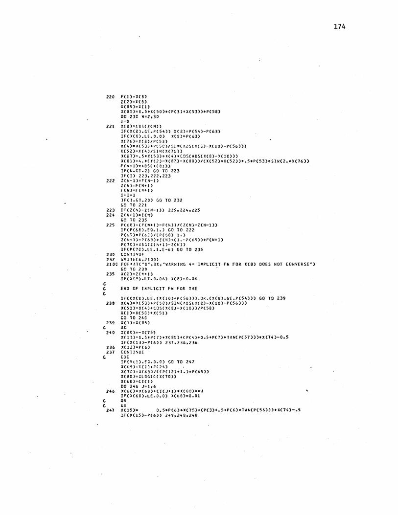
c c c
220
221
222
223 2H
225
230 232 21 oc
235
238
239 c
HO
236 237
c
c c
247
F<l)=X(8) l(2}=X(9} X(85)=X(l} xcss>=c.s~xcso>•<PC3)+XCS3>>•PC58>
DO 230 11=2,30 1=0 X(S)=tSS(l(N)) lf(X(8).GE.P(54)) X(B)=P(54)-P(63) IFCX(8).LE.O.O) X(8)=P(63) X(76)=1(8)/P(53} X(4)=X(53)$P(58)/SlN(AoS(X(S)-X(10)-P(56))) X(52)=X(~)/SlN(X(7~))
X(B7)=.5•1(53)oX(4)*COS(ABS(X(8)-X(10))} XCBl)=~.•(T(2)-X(87)-X(88))/(X(52)oX(52))+.5•PC53)*5lN(2.oX(76)) f(~<l)=l8SCX(8l))
IF{N.GT.2) GO TO 223 IFCI) 223,222,223 l(N-l)=F{N-1) l(h)=F(N+1) F(Pi)=F(N+1) 1=1+1 1F(T.GT.20) GO TO 232 GO TO 221 IF(l(N)-Z(N-1)) 225,224,225 ZOi+l >=ZCN) C.C TO 235 PCcP.)={F(N+1)-f(~))/(Z(N)-Z(N-l))
JF(P(68).EO.l.) GO TO 222 P(bS)=P(6~)/(P(~8)-1.)
ZCN+ll=P(69)>l(~)+(l.-P(69))>f(N+l)
P(7C)=tc~(l(h<l)-Z(N))
IF(P{70).lf.l.E-6) GO TO 235 (~PiTI'iUf
&Q1Tf(6,2100) f0~•&1("0",3X,"WARNING ~= IMPLICIT FN fOR X(8) DOES NOT CONVERSE•) GO TO 239 . xca >=Z<•!~I > lf(~(!).LT.C.06) X{f)=0.06
END OF lXPllCIT FN FOR THE
1FCCICB>.LE.(X(l0)+P(56})).0R.{X(8).GE.PC54))) GO TO 239 X(4)=1(53)~P(58)/SI!i(IBS(X(8)-X(l0)-P(56)))
XC5l)=X(~)*COS(X(8)-X(l0))/P(58)
X(l)=X(50)+X(51) GO TO 2~0 X(l)=X(85) AC X( 80)=-X(75) XC13)=0.So?(7)•X(80)+{P{4)+0.5+P(7)*TAH(P(57)))*X(74)-0.5 IF{X(l3)-P(6)) 237,236,236 X(13)=PC6) CONll'iUE ([)(
IF(Jt!).f:.C.C) GO TO 2~7
l(69)=Y(l)•PC?~)
XC7Cl=XC69)/((?{J2)+1.)•P(65)) X(aO>=~LOGlG(X(70))
l((,f)=(I(l) DO H6 J=l,6 XC6E)=X(68)+CI(J+1)•XC60)•~J
Jf(XC68).LE.O.Q) X(68)=0.01 OB AB XC15)= 0.5•P(6)~X(75)+(P(3)+.5+P(6)•TAN(P{56)))$X(74)-.5
lf(X(15)-P(6)) 249,2~8.248
174

H8 X(l5)=P(6) X(18)= P(6)*SORT(-X(21)) X(36)=X(21) 104=1 GO TO 250
249 X(18)=X(15)oSQRT(-X(21)) X(36)=-(X(18)/P(6))**2 IF(X(15).GE.O.SO•P(6)) 104=1
250 CONTINUE GO TO 300
295 X(79)=X(32) 300 CCNTI NUE C •••• OUIOIT TMOATA : PTC=0.41
$0AHAJN NT=~• NP=72, HX=88, OELT=1.5, PROEL=3.0, E NOTIII=l 000., IRK=4, Yl(I)=0.0,2.0,2.0,-1.5E-lo P(4l)=0.41, P<n=t.o. P<30=17.2285, P(3)=0.S, P(l1)=9.6B7, p(31)=19.3H, P(9)=ll.O, P0)=12.0, P(2)=12.0, P{S)=C.C, P<O=l.O, PC1>=2.o, P{8)=3. OS, P{ 10)=10. 9U, P(36)=10 •. 9t,2, P(12)=1C.O, P(13)=32.3~,
P(14)=32.34, P(15)=5.5, PO 6)=0.1, P(17)=3. 075, P(l8)=10.5, P(19)=2-360E-2, P(20)=1.123E-7, P(22)=230.6872, P(23)=2308.8715, PC2io>=97eJ.o, P{ 33)= 19. 8090, TABLEl=-29,-20,1,-2,3,-31,-6,-32,/oo ~LOTl=-29,1,-20,
SEND
175
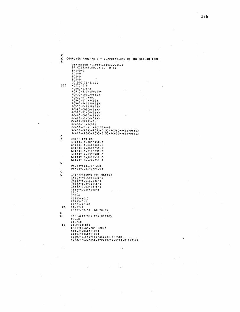
c C CO~PUTER PROGRAK 3 - COKPUTATIONS OF THE RETURN TIME c
Dl~~~SION FC10l) 0 Z(l0l),Cl(7) IF <ISTART.EQ.O) GO TO 50 IFI'IO=O IDl=O 102=0 103=0 DO 500 II=l,IOO
500 X(Jl)=O.O
c
P(SC)=l.E-3 P(51)=3.14159265~
P(52)=1BO./P(51) PC5~)=67./90. P(54)=67./P(52) P(56)=P(l)/P(52) PC 5 7)=f'( 2)/P( 52) PCSS)=COS(P(56)) P(5S)=SlN(P(56)) P(tC)=CGSCPC57)) PC61)=S!N(P(57)) PC62)=?(15)/3. f(63)=1./P(52) P(o~)=(l.~l./P(17}}**2
X(65)={P(3)-P(5)+0.5)*P(58)+P{9)*P(59) X(66)=(P(~}+P(5)~0.5)•P(60)+P(9)~P(61)
C COEFF FOR CO CJ(l)= 6.905645E-2 C!C2)= 2.0675JGE-l CIC3)= 2.064! ZSE-1 CIC~l=-5.8143Q9f-2 CIC5)=-7.13939CE-2 CIC6>= 4.834454E-2 CIC7)=-8.~77535E-3
c
c
PC2~)=P(l6)/P(23) P(~2)=l.S£-3/PC26)
C ITERA?ATJDWS FOR OCCTO) X(l0)=-2.688563£-1 X(l3l=E.Ol8~93E-l X(28)=1.8S7294E-l XC66)=7.934~37E-l l(l)=~.O~S499E-l
IT=C I~S:O
xco6l=HO X( la)=0-2 l(E';}=T.( 18)
eo IT=IT~l IFCIT.GT.S) GO TO 85
t t !~!?,~AllONS FOR QB(TO)
hC~=O
lli:F=O 10 IH~=IHR+l
lf(ITfR.GT.ZO) NCR=2 X(74)=CQS(X(l0)} X(75)=Sih(X(10)) l(50)=0.5C(P(6)+X(75)) /P(58) XC53J=~(3)+X(SO)•P(59)+0.5~(l.O-X(7~))
176
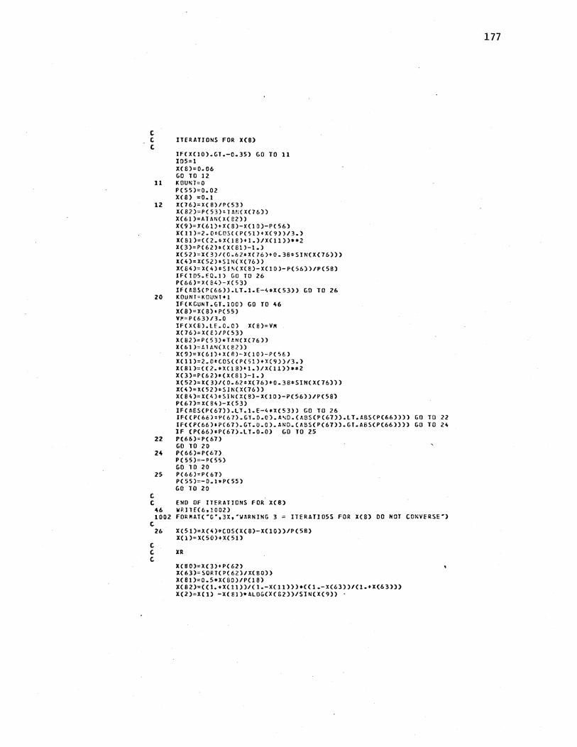
c C ITERATIONS FOR X(8) c.
c c
IFCXC10).GT.-0.35) GO TO 11 105=1 XC 8)=0. 06 GO TO 12
11 KOUt;T=O P(55)=0.02 XC8) =0.1
12 X(76)=X(8)/P(53) X(82)=PC53)•TIN(X(76)) XC61)=ATAN(X(82)) X(9)=X(61)+X(8)-X(10)-P(56) XC11)=2.0~COS((P(Sl)+X(9))/3.}
X(81)=((2.~X(18}+1.)/X(ll))**2 X(3)=PC62)~(X(81}-1.)
X(5?)=X(3}/(C.62~X(76)+0.38~SIN(X{76)))
X{•)=XC52)tSIN(X(76)) X(6~)=X(4)~SJ~(X(8)-X(l0)-P{;6))/P(58)
JF(105.f0.!) GO TO 26 P(66)=X(84)-X(53) If(~BS(P(66)).LT.1.E-4*X(53)) GO TO 26
20 KOUNT=KOUNT+l JF(KCUNT.GT.lOO) GO TO ~6 X(8)=X(8)+P(55) V~=P(63)13.0
JF(X(S).LE.O.O) X(8)=VM XC76)~XCE)/P(53)
X(82)=P(53)•TtN(X(76)) XC6l)=~lAN(X(82))
XC9)=X{61)+X(8}-X(l0}-P(5~)
X(11)=2.0~COSCCPC5l)+X(9))13.) X(81)=((2.•XC18)+1.)/X(1l))••2 X{3)=P(62)o(X(81)-l.) X(52)=X{3)/(0.62~X(76)+0.38~SJN(X{76)))
X(4)=X(52)•SIN(X(76)) XC84)=X(4)~SIN(X(8)-X{l0)-P(56))/P(58)
P(67)=X(84)-X(53) IFCAES{P(67)).LT.l.E-4•XC53)) GO TO 26 IF{(P(66)$P(67).GT.O.C).A~O.(ABS(P(67)).LT.ABSCP(66)))) GO TO 22 IF((P(66)t?(67).GT.O.O).AND.(ABS(P(67)).GT.A8S(P(66)))) GO TO 24 IF (P(66)$P(67).LT-0.0) GO TO 25
22 P(66)=P{67) GO TO 20
24 P(66)=P(67)
25
P(55)=-PCSS) GO TO 20 PC66)=PC67) PC55)=-0.l*P{55) GO TO 20
46 1002
c
ENO OF ITERATIONS FOR X{8) WP.IT£(6,1002) FOR"AT("Q",3X,"W~RNING 3 = ITERATIOSS FOR X(8) DO NOT CONVERSE")
c c c
26 X(5l)=X(4)~COS(X(8)-XC10))/P(58)
X(l)=X(50)+X(51)
XR
X(BO)=X(3)+P{62) X(63)=SORT(P(62)/X(80)) X{81)=0.5vX(80)/P(l8) X(82)=((1.+X(ll))/(l.-X(ll)))•{(l.-X(63))/(l.+X(63))) X(2)=X(l) -X(81)*ALOG(X(S2))/SlN(X(9)) ·
177

c c Rtl t
X(3l)=0.5•XC52)/P(53) X(80)=X(37)+0.5 X(2l)=P(9)-0.5•PC6)-X(8Q)~X(75) X(8Z)=X(20)*X(7~)-P(S)
X03)=ATAk(X(8l )/X(82)) X(35)=0.5•(X(l0)•X(33)) XC~C)=2.•X(37)oX(35)
XCBl)=X(~Q)+?(62)
X(41)=50Rl(P(62)/XC81)) X(~2)=(.5tX(8!)/P(l8))*ALOG((l.+X(41))/(l.-X(41)))
XCB2)=0.5-XC42) X{33)=CDSC2.~X(35))-l.O
X(5)=X(37)+.5*(l.•XC82)o{2.•XC37)+X(82))/CXC37)•XC83)-X(82))) lf((X(S}-1(37))-20.0) 17o1Sol5
15 X(S)=X(80) c; C ET Jl2 • SS c
c
17 XC6!)=P(9)-0.5•P(6)-X(5)oX(75) X(t2)=X(5)•XC7~)-P(5) XC62)=ATAN(X(8l)/XC82)) X(57)=X(5)•(X(l0)+X(62))
C OE2 c;
X{l6)=0.5•CSCRT(l.+X(57)1P(62))-1.) c C PJ c.
t
X(83)=X(l~)-l(l) lF(X{e3).lE.O.G) XC83)=0~0 XCS2)=P(8)+X(66) X(22)= -(X(23)/X(82))**2 X(2J)=X(22)-2.01X(5) lF(X(2l).GE.Q.O) X(21)=-0.02
t AB C OB t
104=0 1(15)= 0.5oP(6)oX(75}+(P(3)+.5+P(6}*lAN(P(56)))•X(7~)-.5
lf(X(15)-P(6)) 31 0 30,30 30 )((15)=?(6)
X(lS)= P(6)*SCRT(-X(21)) XC36):X(21) ID~=l GO TO 32
31 XC1e)=XC15)~~0RT(-X(21))
X(36)=-(X(l8)/P{6))*•2 lF{1(15).GE.0.80 •PC6)) ID~~l
32 (~NTl~UE ' JF(~~S(X{l8)-X(85)).lf.P(50)) GO TO 82 GO TO 27
82 -1iCI<=3 C AC
lt( 80 )=-X(75) X(!3)=C.5•P(7)•XC80)+(P(~)+0.5+P(7)*TAN(P(57)))oX(7~)-0.5 !F(X(l3)-P(7)) 36 0 35,35
35 X(l3)=P(7) 36 CONTINUE
c oc l(81)=l./X{l3)oo2+(P(35)-l.)IP(7)o•2~1./(X(68)•P(7))**2 Y(l)=SCQT((P(~l)-X(22))1X(81})
178
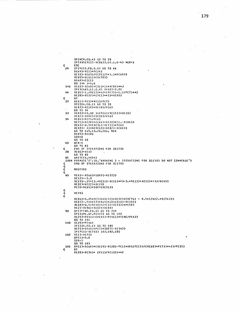
c 29
146
c 21
33
c 28
as 100~
c c c c
c c c
~5
so
100
182
101 c
IF(NCR.EO.~) GO TO 29 lF(ABS(Y(l)-X(86)).LE.l.E-~) NCR•l CDC lF(Y(l).EO.O.Q) GO TO~~ X(69)•T(l)*P(2~)
X(70)=X(69)/((P(12)+l.)*PC65)) X(80)=Al0G10(X(70)) X(68)=Cl(l) DO 146 J=lr6 X(68)•X(68)+Cl(J+J)oX(80)**J IF(X(68).LE.O.O) X(68)•0.01 X(80)=1./X(13)•~2+(P(35)-l.)/P(7)oo2 X(28)•X(22)+(Y(1)oo2)oX(80) BT X(81)=T(1)oT(l)/P(7) 1F(I04.E0.1) GO TO 33 XC82)=X(18)~X(l8)/P(6)
GO TC 3~ X(80)=(0.80 )~(P(6)/X(15))~X(l8) X{82)=X(8v)*X(30)/P(6) X(84)=P(7)/P(6) X(7l)=X(28)~X(84)+X(22)o(l.-X(8~))
X(E3)•0.5~(X(36)-X(7l))*P(6) X(lO)= tlAN(X(S3)+X{82)-X(81)) GO TO {~5,43,28,28), NCR XC85)=X(18) 105=0 GO TO 10 NCR='t GO TO 82 END OF ITERATIONS FOR OBCTO) X( 86)=Y( 1)
GO TO 80 WRilE{6,100n FOR~AT("0",3X,·~~RNING 2 = ITERATIONS FOR OC(TO) 00 NOT CONVERGE") END OF ITERATIONS FOR OCCTO)
.00200)
Y(~)=-X{66)~SORT(-X(22))
X(l2)•-1. 0 X(23)=.25~(3.•XC11)-X(ll)•*3-3.•X(l2)+X(l2)*~3)/X(65) XC3l)=XC2.2)+X(23) J(3)=X(65)•SORT(X(31))
V(TO)
X(86)=0.2S•P(53)•XC52)oX(52)o{X(76} - 0.5~SIN(2.oX(76)))
X(87)=.5*X(53)•X(4)•COS{X(8}-X(10)) X(88)•0.5~X(5Q)o(P(3)+X(53))*P(58)
YCZ)=X(86)+X(87)+XCBB) IF(IfiNO.EO.l) GO TO 100 IF(Tlr.E.Gf.P(42)) GO TO 100 X(29)•P(~l)-{P(~l)-P{~6))oTI~E/P(t,l)
GO TO 101 X(.29)•P(46) IFCIDI.EQ.l) GO TO 180 X(73)=X(68)•P(7)~SQRT(-X(3~))
1F(Y(l)-X(73)) 182,182.101 T(l )•X(73) OT(l )=0.0 101=1 GO TO 183 0T(l)=X(68)o(X(29)-X(28)-T(l)oABS(T(l))/(X(6S)oP(7))o*2)/P(31) BT X(28)=X(34)+ (T(l)/X(13))oo2
179
XC8l)=J(l)*Y(l)/P(7) IF(J04.EO.l) GO TO 186 X(8Z}=X(18)oX(18)/P(6) GO TO 167
186 1(80)=(0.80 )tCP(6)/X(15))tX(18) X(BZ):X(f0)tX(80)/P(6)
187 X(8~)=P(7)/P(6)
X(71)=X(28)oX(84)+X(34)t(l.-X(84)) X(83)=0.5o(X(36)-X(7!))oP(6) X(lOJ= ~Tt~(X{83)+X{82)-X(81)) GO TO 181
160 J(l):X(6o)tP(7}oSORT(-X(3~))
183 IF(l04.EC.l) GO TO !84 X(E2)=X(IB)tX(l8)/P(6) GO TG B5
184 1(80)=(0.30 )*{P(6)/X(15))oX(18) XC&Z)=X(oQ)oX(EC)/?(6)
185 X(E3)=C.5o(X(36)-X(34))~P(6) X(!C)= tlA~(X{a3)+X(82))
lol ~(74)=~cSCX(IC))
X(7;)=~1~(X(!C))
XC50)=G.5o(P(6)+X{75)) /P{58) X(53)=P(3)+X(5~)oP(59)+C.5t(1.0-X(74))
XC51)=X(1)-l{50) X(8l)=(X(51)oP(59)•X(53))tt2+(X(5l)oP(58))tt2 XC4)=SO~T(X(81})
IF(J(lO).GT.-0.35) GO TO 190 xce>=o.n G:l TO 191
!90 XCE!)=J(5~)o?(5?)/I(~)
J(e)=!,S!N(~{8!))+XC1C)•P(56) 191 xc7l>=xcc>J~C53)
XCB2}:P(5])eT~h(X(76))
X(bl)=:.T.t.N(X( 32))
X(9)=X(61)•J(8)-X(10)-P(56) C. RCL
XC52)=l(~)/SIN(X(76))
X(37)=0.5$X(52)/P(53) X((;!l)=X(37)+0.5 X(&l)=P(9)-C.5~P{6)-X(30)eX(75)
xcaz>=XC80>•XC7~l-PCS> X(33)=!Tt~(X(Bl)/X(82))
X(35)=C.~•(X(l0)+X(33)) C. SP
X(40)=2.•X(37)•X(35) c fp
X(3l)=X(~O)+P(o2)
X(~li=SC~T(?(62l/X(81))
X(~2)=(.So~(RI)/P{l8))~1LOG({1.+X(~l))/(l.-X(~l))) Ha2J=o.s-x<42) X(83)=COS{Z.~xc;S)}-l.Q
X(5)=X(37)T.5e(l.+X(B2)~(2.eX(37)+X(82))/(X(37)eXC83)-X(82)))
IF((X(5)-XC37))-20.0) 189.188.188 181! xn>=xcao>
c f1A'l l89 X(cl)=PC91-C.SeP(6)-X(5)•X(75)
X(c2)=l(5)•X(74)-P{5) X(62)=.t.T~~{X(cl)/X(SZ))
C. YSP X(83)=X(ol)•$2•X(82)•$2 1{6C)=$CRT(X(83)) 1(6);X(5)-X(60)
C SSP X(57)=X(5)~(X(10)+X(62))
(; TS XC8C);P(1E)•X(6)/(X(57)+P(6Z))
180

c c c
lOZ
172
173
lH 103
104
161
162 163
164
165
175
176 117
107
166
167 168
108
169
X(81)=EXP(X(BO)) X(82)=EXP{-X(80)) X(l2)=(X(81)-X(82))/(X(Bl)+X{82)) SPliTTER EFFECT xc77>=<t.-l.s•x<IZ>•.s•x<1Z>••3>•coscxc9>>+1.+1.S•xctz>-
1 0.50X(I2)*•3 XC78)=ARCOSCX(77)12.) X(11)=2.0•COS((P(5l)+X(78))/3.) PBE X(8l)=X(68)•PC7) lf(X(10)) 164,16~,102 X(62)=X(S)oX(75)+.5oP(6) X(83)=PC36)•P(60) 1F(X(82)-X(83)) 172,172,173 X(~6)=X(5)~X(10)
X{~7)=1.825*(X(~6)+PC62))/P(18) X(38)=X(82)*TAN(P(57))+P(4)+.5-X(5)o(1.-X(7~))-X(47)
GO TO 1 H X(47)=1.825*(X{46)+PC62))/P(18) X(38)=P(36)*P(6l)+P(4)+.5-{X(6)-P(5))-X(~7)
IF(X(3c)) 103,103,104 X0£)=0.0 X<~O=O.O GO TO 163 X(SC)=X(22)-X(34) lf(X(80)) 162,161,161 X(44)=X(3S)~SQRT(X(80))
GO TO 163 X(44)=-X(38)•SO~T{-XCS0)) X(43l=O.S•CSQRT(l.<X(,6)/P(62))-1.) X(83)=Y(l) +X{44)-X(43) X(S4)=X(81)+X(38) X(3~)=X(34)+X(83)•1BS(X(83))/X(S~)*•2
Jf(X(3~)~GE.0.0) X(3~)=0.0 GO TO 165 X{~6)=0.0 :X(H)=0.5 XCHl=X(22) X{H)=-Y(l) X(B)=O.O X(38)=X(8l)
PDZ 002 X(23)=.25•<3-*X(ll)-X(ll)**3-3.•X(l2)+X(12)**3)/X{65) X(3l)=X{22)+X{23) X(2~)=.25v(2.+3.•XC12)-X(l2)~•3)/X(66) X(32)=XC22)+X(2~)
lF(X(57)-X(46)) 175.176,176 X(S2)=X(~6}
(;0 TO 177 X(82}=X(57) X{45)=0.5•<SORT(l.+X(62)/PC62))•1.)-X(~3)
OY(~}=(X(32}-X(26)-T(4)•A9S{Y(~))/X(66}*~2)/P{3~)
JF(Y(4}) 107,!08.108 XCS2}=P(8)¢SQRT(-X(22))-Y{4)-X(4~}-X(~5)
lf{X(~4)) 166,167,167 X(c3)=P(B)+X(66)+X(38) GO TO !68 X(83)=P(8)+X(66) X{17)=XC82)~AB~{X(S2))/X(S3)•o2
GO TO 109 X(82)=P(8)~SORTC-XC22))-X(4~)-X{~5)
IF(X(~4}} 169.170,170 X(ti3)=P(8)+X(38} GO TO 171
181

170 X(B3)=P(8) 171 X(l7)=X(82)oASS(X(82))/X(83)o•2
C POUT XC20)=(Y(4)fX(66))o•2
t 109 X(22)=XC22)+X(l7)
IFCXC22).GE.0.0) X(22)=0.0 t P1
X(EJ);X(~~)IX(57)
XC21)=X(Sl)tX(3~)+(1.-X(8l))oX(22)-2./X(5).
c XI! X(3)=X(52}c(C.62oX(76)+0.38oSIN(X(76))) X(8C)=X(3)+P(62) X(63)=SORT(P(62)/X(80)) X(81)=0.5tX(80)1P(18) X(82)=((!.+X(ll))/(l.-X(Il)))o{(l.-X(63))/(l.+X(63))) X(l)=7(l) -X(8l)•tl0G(X(82))/SIN(X(9))
C OY/DT
'
IF(X(2)-P(lC)) 11C.ll0.111 110 0T(2}=X(JB)~O.Sc(}.-X(ll)/X(63))
XCl~)=C.O
X(l9)=0.0 GO TO 1!7
111 IF(I02.f0.1) GC TO 116 X(8!)=P(lO)•P(5B)-X(5)oX(75)-0.5oP(6) XC&2)=X(5}•X(74)-P(1Q)oP(59)-(P(3)+0.5) X(3S)=AT~~(X(8l)/X(82))
IFCX(39)-P(56)) 112.112.113 112 I::;2=1
GO TC ll5 113 ~CSS)=X(~}o(~(l0)+~C39))
X(59)=1.825•(XC5E)tP(62))/?(l8) X(1~)=X(S)-X(59)-X(81)/SlH(X(39))
IF(X(1~)) 110.110.11~ 11~ 1F(X(11}-P(8}) 116oll5.115 115 XCIO=P(8) 116 X(l9)=X(l~)oSORT(-X(21))
0Y(2)=X(l8)+0.5t(l.-XC11)/X(63))+X(l9)
C l~?LICIT FN FOR THE c:
117 IF(YCIO).GT.-0.35) GO TO 120 X(8}=0.06 GO TO 138
120 F(l)=X(8) ZC2l=JCE> XCBS):X(l) X(8e)=L.~•X(SO)o(P(3)+X(53})oP(58) D'l 133 1;=2, 3C i=O
121 X{Z)=A95{ZCH)} 1F(X(8).GE.P(5~)) XC8)=P(54)-P(63) lF(X{S).lf.O.O) X(8)=P(63) X(16)=X(8)/P(53) l(4):X(53)tP(52)/SIN{AaS(X(8)-X(l0)-P(56))) X(52)=X(~)/SIN(XC76))
XCS7)=.5~X(53)oX(~)•COSCAE5(X{8)-X(l0))) X(ol)=~.t(Y(2}-X(&7)-X(88))/(X(52)~X(52))+.5~P(53)vSIN(2.oX(76))
f(N+l)=!ES(X(B!)) IF{N.GT.2) GO TO 123 IF{l) 123,122.123
122 Z(N-l)=F<N-1) l(N)=F(N~l)
FCN)=F(N+l) 1=1+1 IFCI.GT.ZO) GO TO 132
182

GO TO 121 123 1F(l(N)-Z(N-1)) 125.12~.125 12't Z(N+l)=l(N)
GO TO 135 125 P(68)=(F(N+1)-F(N))/(Z(N)-l(N-l))
1F(P(68).EO.l.) GO TO 122 P(69)=P(68)/(P(68)-I.) l(N+l)=P(69)~Z(N)+(l.-P(69))*f(N+l)
P(70)=AB$(l(Nfl)-Z(N)) IF(P(70).LE.l.E-6) GO TO 135
130 CONTINUE 132 WRITEC6.Il00) 1100 FOR~AT("0"•3X."WARNING ~=IMPLICIT FN FOR X(S) ODES HOT CONVERSE")
GO TO 139 135 XCS)=Z(N+l)
IF(X(8).LT.0.06) X(8)=0.06 c C END OF IMPLICIT FN FOR THE c
IF((X(S).Lf.(X(l0)+P(56))).0R.(X(8).GE.P(5~))) GO TO 139 138 X(4)=X(53)~P(56)/$IN(ABS(X(8)-X(10)-P(56)))
X(5l)=X(4)$(0S(X(8)-X(l0))/P(58) X(l)=X(50)+X(51) GO TO HO
139 X(l)=X(85) C AC 1~0 X(80)=-X(75)
X(13)=0.5tP(l)*X(80)+(P(~)+0.5+P(7)*TAN(P(57)))~X(7~)-0.5 IF(X(l3)-P(7)) 137.136.136
136 X(13)=P(7) 137 CONTIOJUE
C CDC IF(Y(l).fO.O.O) GO TO 1~7 X(b9)=Y(l)*P(2~)
X(70)=X(69)/((P(l2)+1.)•P(65)) X(80)=Al0Gl0(X(70)) XC68)=C.l(l) DO lio6 J=1•6
1~6 X(6S)=X{6E)+C.I(J+l)•XCSO)~*J IF(XC6S).LE.O.O) X(68)=0.01
c Q!l C AB
c
1~7 X(l5)= 0.5*P(6)*X(75)+(P(3)+.5+P(6)*TAN(P(56)))~X{7~)-.5
IF(X(15)-P(6)) 1~9.1~8.1~8 H8 X(15}=P(6)
X(l6)= P(6)•SORT(-X(21)) X(36)=X(21) 10~=1 GO TO 150
1~9 X(18)=X(l5)*SOR1{-X(21)) 149 X(lB)=XCI5)~SQRTC-X{21))
X(3b)=-(X(l8)/P(6))**2 lf(X(15).GE.0.80#P(6)) 104=1
150 CONTINUE
C SWITCHING IF(l03.EC.1) GO TO 155 lF(X{6}.LE.O.O) GO TO 195 X(7)=C.95$X(66)*SORT(X(79)) 103=1
155 IF(Y(4).LT.X(7)) GO TO 200 IFIND=l E NOT IM=TIPIE ~RITEC6.160)P(~l).T!ME.X(18)•Y(4).X(7).X{6).X(20)
160 FDRPIAT("0"•3X.Fl6.5.Fl6.3.1P5E16.6) GO 10 200
183
195 XC79)=X(32) 200 (.OhT H<UE
( •••• DU~MY T~ D~TA : PTC=C.~S IN , 02=1.0 SOAT~I~ ~Y=~, ~P=72, NX=88, DELT=l.O, PROEL=~.O, fi•!JTI!i=SOO.O, IRK=2o Tl(l)=3.751~58E-1,6.676356,0.0,-3.63131BE-2,
P(t,l)=0-"5• P(t,}=O.S, PC12>=9.687, H 31)=19. 3H, P(3"}=19.8090, P(3)=1.0, PC32}=llt.Oll6o P(9)=11.Cr P(l )=12.0, P<S>=C.O, P(6)=2.C, PC7l=l.O, PC8)=3.CS, P(l0l=JC.942, PC36)=10.'H2, P(ll)=IQ.O, P(l3)=32.34, P(l")=32.3.r,, :>(15)=5.5, P(I6)=C.l, P(l7)=3. 075, 1>(18)=\C.S, P{l9)=2.3bOE-2t P(20)=l.l23E-7, P ( 22)= nc·. a en. PC13)=23C8.a715, 1>(24)=9783.0, P(.r,b)=C.O, G~Ul(3)=!.0,
~:.~<lxt<4>=:.o,
GP~I~H3}=1.0o
G~l~l(4)=J.O, . iLBLEl= 1,101,-2,-18,-10,-1~,-19,-6,-32,~, PLO!l=l,2 1 -3l,-32,-20o
SEND
184

ENDNOTE
1J. H. Wegstein, "Accelerating Convergence of Iterative Processes," Communications of the Association for Computing Machinery, 1, 6 (June, 1958), pp. 9-13-. -
185

;'1
VITA d.
Hyo Whan Chang
Candidate for the Degree of
Doctor of Philosophy
Thesis: DYNAMIC ANALYSIS OF A MONOSTABLE FLUID AMPLIFIER
Major Field: Mechanical Engineering
Biographical:
Personal Data: Born in Chulwon, Korea, March 22, 1945, the son of Mr. and Mrs. Sung Ryong Chang.
Education: Graduated from Seoul High School, Seoul, Korea, in 1963; received the Bachelor of Science in Engineering degree in Mechanical Engineering from Seoul National University, Seoul, Korea, in 1968; received the Master of Science degree in Mechanical Engineering from the State University of New York at Buffalo, New York, in 1972; enrolled in the Systems Engineering doctoral program at Case Western Reserve University, 1972-73; completed requirements for the Doctor of Philosophy degree at Oklahoma State University in July, 1978.
Professional Experience: Ordnance Maintenance Officer, Korean Army, 1968-70; graduate research assistant, State University of New York at Buffalo, 1970-72; Laboratory Instructor, Systems Engineering Division, Case Western Reserve University, 1972-73; graduate research assistant, Oklahoma State University, 1974 to date.
Professional Affiliations: American Society of Mechanical Engineers; Korean Scientists and Engineers Association in America.
Recommended