Louisiana State UniversityLSU Digital Commons
LSU Doctoral Dissertations Graduate School
2012
Dynamic characterization of vocal fold virbrationsZhenyi WeiLouisiana State University and Agricultural and Mechanical College, [email protected]
Follow this and additional works at: https://digitalcommons.lsu.edu/gradschool_dissertations
Part of the Mechanical Engineering Commons
This Dissertation is brought to you for free and open access by the Graduate School at LSU Digital Commons. It has been accepted for inclusion inLSU Doctoral Dissertations by an authorized graduate school editor of LSU Digital Commons. For more information, please [email protected].
Recommended CitationWei, Zhenyi, "Dynamic characterization of vocal fold virbrations" (2012). LSU Doctoral Dissertations. 1799.https://digitalcommons.lsu.edu/gradschool_dissertations/1799
DYNAMIC CHARACTERIZATION OF VOCAL FOLD VIBRATIONS
A Dissertation
Submitted to the Graduate Faculty of theLouisiana State University and
Agricultural and Mechanical Collegein partial fulfillment of the
requirements for the degree ofDoctor of Philosophy
in
The Department of Mechanical Engineering
byZhenyi Wei
B.S., Zhejiang University, China, 2001M.S., Zhejiang University, China, 2004
August 2012
Acknowledgments
I would like to express my deepest gratitude to my advisor, Dr. Marcio de Queiroz,
for his patient guidance and continuous support during my graduate years. His ex-
pertise, insight, and quest for perfection in research greatly impressed me and
added great value to my research experience. Without his guidance, I would have
never finished this dissertation. I would like to thank my committee member,
Dr. Melda Kunduk, who guided me in this specialized medical area. Her knowledge
in voice disorders and experience in clinical practice greatly help me understand
the nature of vocal folds. I would also like to thank my collaborator, Jing Chen, for
her wonderful work in pre-processing the raw data captured from the high-speed
digital imaging system.
Gratitude is extended to all my friends, especially to An Wu and Ziliang Cai,
for their help over the years. I would like to thank my parents and brothers for
their support and encouragement. Last but not least, I would like to thank my
wife, Jiongjiong for standing beside me.
ii
Table of Contents
Acknowledgments . . . . . . . . . . . . . . . . . . . . . . . . . . . . . . . . . . . . . . . . . . . . . . . . . . . . . . . . . . . ii
List of Tables . . . . . . . . . . . . . . . . . . . . . . . . . . . . . . . . . . . . . . . . . . . . . . . . . . . . . . . . . . . . . . . v
List of Figures . . . . . . . . . . . . . . . . . . . . . . . . . . . . . . . . . . . . . . . . . . . . . . . . . . . . . . . . . . . . . . vi
Abstract . . . . . . . . . . . . . . . . . . . . . . . . . . . . . . . . . . . . . . . . . . . . . . . . . . . . . . . . . . . . . . . . . . . . x
Chapter 1: Introduction . . . . . . . . . . . . . . . . . . . . . . . . . . . . . . . . . . . . . . . . . . . . . . . . . . . . 11.1 Motivation . . . . . . . . . . . . . . . . . . . . . . . . . . . . . . . . 11.2 Vocal Fold Anatomy . . . . . . . . . . . . . . . . . . . . . . . . . . 31.3 Voice Production . . . . . . . . . . . . . . . . . . . . . . . . . . . . 61.4 Voice Disorders . . . . . . . . . . . . . . . . . . . . . . . . . . . . . 71.5 Vocal Fold Examination . . . . . . . . . . . . . . . . . . . . . . . . 81.6 Scope of Work . . . . . . . . . . . . . . . . . . . . . . . . . . . . . . 10
Chapter 2: Biomechanical Models of Vocal Folds . . . . . . . . . . . . . . . . . . . . . . . . . . . 122.1 One-Mass Model . . . . . . . . . . . . . . . . . . . . . . . . . . . . 122.2 Two-Mass Model . . . . . . . . . . . . . . . . . . . . . . . . . . . . 132.3 Multi-Mass Models . . . . . . . . . . . . . . . . . . . . . . . . . . . 182.4 Asymmetric Models . . . . . . . . . . . . . . . . . . . . . . . . . . . 192.5 Estimation Approaches for Model Parameters . . . . . . . . . . . . 21
Chapter 3: Proposed Biomechanical Model . . . . . . . . . . . . . . . . . . . . . . . . . . . . . . . . . 223.1 Basic Nomenclature . . . . . . . . . . . . . . . . . . . . . . . . . . . 223.2 Model Description . . . . . . . . . . . . . . . . . . . . . . . . . . . 23
Chapter 4: Tuning of Model Parameters . . . . . . . . . . . . . . . . . . . . . . . . . . . . . . . . . . . . 294.1 Manual Coarse-Tuning Procedure . . . . . . . . . . . . . . . . . . . 304.2 Automatic Fine-Tuning Procedure . . . . . . . . . . . . . . . . . . . 32
Chapter 5: Results . . . . . . . . . . . . . . . . . . . . . . . . . . . . . . . . . . . . . . . . . . . . . . . . . . . . . . . . . 355.1 Experimental System . . . . . . . . . . . . . . . . . . . . . . . . . . 355.2 Data Processing . . . . . . . . . . . . . . . . . . . . . . . . . . . . . 36
5.2.1 Corrections for FFT Calculation . . . . . . . . . . . . . . . . 375.2.2 Alignment . . . . . . . . . . . . . . . . . . . . . . . . . . . . 38
5.3 Analysis of Results . . . . . . . . . . . . . . . . . . . . . . . . . . . 405.3.1 Comparison of Coarse and Fine Tuning . . . . . . . . . . . . 415.3.2 Discussion . . . . . . . . . . . . . . . . . . . . . . . . . . . . 42
Chapter 6: Conclusion and Recommendations . . . . . . . . . . . . . . . . . . . . . . . . . . . . . . 48
iii

References . . . . . . . . . . . . . . . . . . . . . . . . . . . . . . . . . . . . . . . . . . . . . . . . . . . . . . . . . . . . . . . . . . 50
Appendix A: Parameter Tuning Results . . . . . . . . . . . . . . . . . . . . . . . . . . . . . . . . . . . . 53
Appendix B: Tuning Results Figures . . . . . . . . . . . . . . . . . . . . . . . . . . . . . . . . . . . . . . . 58
Vita . . . . . . . . . . . . . . . . . . . . . . . . . . . . . . . . . . . . . . . . . . . . . . . . . . . . . . . . . . . . . . . . . . . . . . . . 74
iv
List of Tables
5.1 Asymmetry parameters. . . . . . . . . . . . . . . . . . . . . . . . . 46
A.1 Parameters for healthy subjects. . . . . . . . . . . . . . . . . . . . . 54
A.2 Parameters for subjects with polyp. . . . . . . . . . . . . . . . . . . 55
A.3 Parameters for subjects with nodules. . . . . . . . . . . . . . . . . . 56
A.4 Parameters for subjects with unilateral paralysis. . . . . . . . . . . 57
v
List of Figures
1.1 Larynx structure and position. . . . . . . . . . . . . . . . . . . . . . 4
1.2 Superior view of vocal folds. Left: supporting structure; right: supe-rior view. . . . . . . . . . . . . . . . . . . . . . . . . . . . . . . . . 5
1.3 Left: frontal view of the left larynx. Right: enlarged view of thecoronal section of the left vocal fold. . . . . . . . . . . . . . . . . . 6
1.4 Schematic of a high-speed imaging system. . . . . . . . . . . . . . . 9
1.5 A typical glottal cycle of vibration of normal (healthy) vocal foldscaptured by a HSDI system. . . . . . . . . . . . . . . . . . . . . . . 10
1.6 Block diagram of the dynamic characterization scheme for the vocalfold vibration. . . . . . . . . . . . . . . . . . . . . . . . . . . . . . . 11
2.1 Schematic of the one-mass model. . . . . . . . . . . . . . . . . . . . 13
2.2 Schematic of the two-mass model. . . . . . . . . . . . . . . . . . . . 15
2.3 A cycle of the vocal fold vibration. . . . . . . . . . . . . . . . . . . 16
2.4 Schematic of the three-mass model. . . . . . . . . . . . . . . . . . . 19
3.1 Side view of the proposed multi-mass model. . . . . . . . . . . . . . 24
3.2 Top view of the proposed multi-mass model. Only upper masses ofcover layer are shown. . . . . . . . . . . . . . . . . . . . . . . . . . 25
3.3 3-D view of the proposed multi-mass model. . . . . . . . . . . . . . 26
3.4 Simulation results of symmetric vocal folds using the proposed multi-mass model. . . . . . . . . . . . . . . . . . . . . . . . . . . . . . . . 28
4.1 Maximum and minimum displacements in cycle j. . . . . . . . . . . 33
4.2 Flowchart of fine tuning procedure. . . . . . . . . . . . . . . . . . . 34
5.1 Geometry of the glottal contour, glottal axis, and displacement of acontour point. . . . . . . . . . . . . . . . . . . . . . . . . . . . . . . 36
5.2 Contour of the glottis vibration during one cycle. . . . . . . . . . . 37
vi
5.3 IFFT method for frequency correction. . . . . . . . . . . . . . . . . 39
5.4 Parabolic interpolation for time delay estimation. . . . . . . . . . . 40
5.5 (a) Experimental and simulation data before alignment. (b) Exper-imental and simulation data after alignment. . . . . . . . . . . . . . 41
5.6 Plot of Ql/r versus Qa/p and classification of asymmetry plane. . . . 47
B.1 Manual coarse tuning for subject H1: simulation and experimentaltime responses. . . . . . . . . . . . . . . . . . . . . . . . . . . . . . 59
B.2 Manual coarse tuning for subject H1: simulation and experimentalamplitude spectra. . . . . . . . . . . . . . . . . . . . . . . . . . . . 59
B.3 Automatic fine tuning for subject H1: simulation and experimentaltime responses. . . . . . . . . . . . . . . . . . . . . . . . . . . . . . 60
B.4 Automatic fine tuning for subject H1: simulation and experimentalamplitude spectra. . . . . . . . . . . . . . . . . . . . . . . . . . . . 60
B.5 Fine tuning for subject H2: simulation and experimental time re-sponses. . . . . . . . . . . . . . . . . . . . . . . . . . . . . . . . . . 61
B.6 Fine tuning for subject H2: simulation and experimental amplitudespectra. . . . . . . . . . . . . . . . . . . . . . . . . . . . . . . . . . 61
B.7 Fine tuning for subject H3: simulation and experimental time re-sponses. . . . . . . . . . . . . . . . . . . . . . . . . . . . . . . . . . 62
B.8 Fine tuning for subject H3: simulation and experimental amplitudespectra. . . . . . . . . . . . . . . . . . . . . . . . . . . . . . . . . . 62
B.9 Fine tuning for subject H4: simulation and experimental time re-sponses. . . . . . . . . . . . . . . . . . . . . . . . . . . . . . . . . . 63
B.10 Fine tuning for subject H4: simulation and experimental amplitudespectra. . . . . . . . . . . . . . . . . . . . . . . . . . . . . . . . . . 63
B.11 Fine tuning for subject P1: simulation and experimental time re-sponses. . . . . . . . . . . . . . . . . . . . . . . . . . . . . . . . . . 64
B.12 Fine tuning for subject P1: simulation and experimental amplitudespectra. . . . . . . . . . . . . . . . . . . . . . . . . . . . . . . . . . 64
B.13 Fine tuning for subject P2: simulation and experimental time re-sponses. . . . . . . . . . . . . . . . . . . . . . . . . . . . . . . . . . 65
vii
B.14 Fine tuning for subject P2: simulation and experimental amplitudespectra. . . . . . . . . . . . . . . . . . . . . . . . . . . . . . . . . . 65
B.15 Fine tuning for subject N1: simulation and experimental time re-sponses. . . . . . . . . . . . . . . . . . . . . . . . . . . . . . . . . . 66
B.16 Fine tuning for subject N1: simulation and experimental amplitudespectra. . . . . . . . . . . . . . . . . . . . . . . . . . . . . . . . . . 66
B.17 Fine tuning for subject N2: simulation and experimental time re-sponses. . . . . . . . . . . . . . . . . . . . . . . . . . . . . . . . . . 67
B.18 Fine tuning for subject N2: simulation and experimental amplitudespectra. . . . . . . . . . . . . . . . . . . . . . . . . . . . . . . . . . 67
B.19 Fine tuning for subject N3: simulation and experimental time re-sponses. . . . . . . . . . . . . . . . . . . . . . . . . . . . . . . . . . 68
B.20 Fine tuning for subject N3: simulation and experimental amplitudespectra. . . . . . . . . . . . . . . . . . . . . . . . . . . . . . . . . . 68
B.21 Fine tuning for subject N4: simulation and experimental time re-sponses. . . . . . . . . . . . . . . . . . . . . . . . . . . . . . . . . . 69
B.22 Fine tuning for subject N4: simulation and experimental amplitudespectra. . . . . . . . . . . . . . . . . . . . . . . . . . . . . . . . . . 69
B.23 Fine tuning for subject U1: simulation and experimental time re-sponses. . . . . . . . . . . . . . . . . . . . . . . . . . . . . . . . . . 70
B.24 Fine tuning for subject U1: simulation and experimental amplitudespectra. . . . . . . . . . . . . . . . . . . . . . . . . . . . . . . . . . 70
B.25 Fine tuning for subject U2: simulation and experimental time re-sponses. . . . . . . . . . . . . . . . . . . . . . . . . . . . . . . . . . 71
B.26 Fine tuning for subject U2: simulation and experimental amplitudespectra. . . . . . . . . . . . . . . . . . . . . . . . . . . . . . . . . . 71
B.27 Fine tuning for subject U3: simulation and experimental time re-sponses. . . . . . . . . . . . . . . . . . . . . . . . . . . . . . . . . . 72
B.28 Fine tuning for subject U3: simulation and experimental amplitudespectra. . . . . . . . . . . . . . . . . . . . . . . . . . . . . . . . . . 72
B.29 Fine tuning for subject U4: simulation and experimental time re-sponses. . . . . . . . . . . . . . . . . . . . . . . . . . . . . . . . . . 73
viii

B.30 Fine tuning for subject U4: simulation and experimental amplitudespectra. . . . . . . . . . . . . . . . . . . . . . . . . . . . . . . . . . 73
ix
Abstract
An emerging trend among voice specialists is the use of quantitative protocols for
the diagnosis and treatment of voice disorders. Vocal fold vibrations are directly
related to voice quality. This research is devoted to providing an objective means
of characterizing these vibrations. Our goal is to develop a dynamic model of
vocal fold vibration, and map the parameter space of the model to a class of voice
disorders; thus, furthering the assessment and diagnosis of voice disorder in clinical
settings.
To this end, this dissertation introduces a new seven-mass biomechanical model
for the vibration of vocal folds. The model is based on the body-cover layer concept
of the vocal fold biomechanics, and segments the cover layer into three masses
along the longitudinal direction of the vocal fold. This segmentation facilitates
the model comparison with the motion of the vocal glottis contour derived from
modern high-speed digital imaging systems. The model simulation is compared to
14 sets of experimental data from human subjects with healthy vocal folds and
pathological vocal folds including nodule, polyp, and unilateral paralysis. We also
propose a semi-empirical two-stage procedure for tuning the parameters so that
the model response matches as closely as possible the experimental data in the
time and frequency domains. The first stage involves the manual coarse tuning of
parameters based on limited data to expedite the process. The second stage is an
automatic (or manual) fine tuning process on a subset of the parameters tuned in
the first stage based on a larger amount of data.
Once an ‘optimal’ set of model parameters has been identified, two model-based
factors, quantifying the asymmetry between left and right vocal folds and anterior
x
and posterior segments of the vocal folds, are introduced and calculated for each
of the 14 cases. The two factors form an asymmetry plane. Based on the value of
the asymmetry factors for the 14 cases, the plane is subdivided into four regions
corresponding to healthy vocal folds, nodule, polyp, and unilateral paralysis. This
yields a clear visual aid for clinicians, correlating the model parameters to voice
quality.
xi
Chapter 1Introduction
1.1 Motivation
Voice disorders can have significant negative effects on an individual’s quality of
life. For example, they can limit one’s choice of profession or cause loss of work
(temporarily or permanently), especially when the profession requires extensive
use of voice (e.g., teachers, singers, actors, and news reporters). This has financial
and emotional implications not only for the individual but for their family and
society. It is estimated that 3% to 9% of the total population of the U.S. has a
voice disorder. Of the total working population in the U.S., approximately 25%
have jobs that critically require voice use with 3% requiring their voice for public
safety [1]. Therefore, there is a need for objective diagnosis and treatment of voice
disorders induced by vocal abuse/misuse and specific congenital, neuromuscular,
or tumor-related disorders.
Vibration of the vocal folds is the primary source of voice production. Irregularity
in the vocal fold vibrations may contribute to abnormal voice. An emerging trend
in speech research is to correlate the characteristics of the vocal fold vibration
with voice quality [41]. This is important because it can help in understanding the
fundamental phonation mechanism; thereby, establishing a quantitative paradigm
for diagnosing and treating voice disorders.
Presently, clinical procedures are still empirical and subjective. In particular,
they rely on indirect aerodynamic and acoustic tests or direct imaging techniques
(e.g., video stroboscope of the sustained phonation). These techniques can show
changes in vocal fold vibratory characteristics as a disease progresses and as a re-
1
sult of normal aging [3, 14]. However, quantitative and objective parameters that
are directly derived from the vocal fold vibration during phonation are still in their
infancy. This missing information not only prevents a unified concept of what char-
acterizes the normal vocal fold function, but also any objective determination of
the effects of medical, surgical, and behavioral voice therapies. Until recently, the
limitation of laryngeal imaging techniques has been a major contributor to this
problem. Fortunately, recent technological improvements have led to the develop-
ment of high-speed digital imaging (HSDI) systems, which permit visualization of
vocal fold vibration in real time with a capture rate of 2000 to 4000 frames per
second (fps). Studies employing HSDI have demonstrated that this technique gives
more detailed and accurate information about the vibratory patterns of vocal folds
during phonation [7, 9, 12, 20, 22].
The importance of biomechanical models of vocal fold vibration to the study of
voice disorders has been recognized since the late 1950s [10, 16]. The model param-
eters should reflect various laryngeal and pathological configurations for physiolog-
ical and clinical applications [13]. A considerable amount of work has been devoted
to this subject, ranging from lumped-parameter, one- and two-dimensional models
to distributed parameter, three-dimensional models [34, 35]. For instance, linear,
lumped-parameter, one- and two-mass models have contributed to the understand-
ing of vocal fold vibration, especially during normal phonation [16]. The simple
one-mass model [6, 10, 11] assumes a uniform motion for the vocal fold layers and
thus does not accurately model most voice vibrations. The more refined two-mass
model [16, 17, 32] attempts to capture the fact that actual vocal folds have a
wave-like motion from bottom to top. The two-mass model has been used to study
a limited number of irregular vocal fold vibrations [16]. Multi-mass models (i.e.,
three or more masses) have been proposed based on the premise that the vocal fold
2
has two tissue layers with different mechanical characteristics – the body layer and
the cover layer [33, 36]. Such multi-mass models are believed to more likely capture
abnormal vibrations in the vocal fold [27]. Another type of multi-mass model was
proposed in [38] by combining five two-mass models along the anterior-posterior
direction of the vocal fold to account for its longitudinal flexibility.
So far, few studies have attempted to compare clinically-observed vocal fold vi-
brations with model simulations [25]. The limited studies can be attributed to the
difficulty in obtaining and processing images of vocal fold vibrations in real time.
The improved use of HSDI in a clinical setting and the development of image pro-
cessing systems are now allowing further studies investigating the compatibility of
vocal fold dynamic models with direct imaging of the vocal fold vibratory charac-
teristics. This comparison will be of great value in furthering our understanding
of the causes of abnormal vocal fold activities, and in predicting the effects of
treatments on patients with different pathologies.
1.2 Vocal Fold Anatomy
The human vocal folds are located above the trachea and form the narrowest por-
tion of the airway passage, named glottis[34]. The vocal folds are housed inside the
larynx, a movable organ that is strengthen and upheld by cartilages and surround-
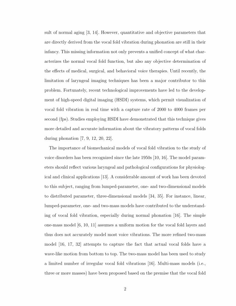
ing muscles. Figure 1.1 shows the sagittal view of the head and neck. From top to
bottom, the nasal cavity, oral cavity, pharynx, vocal folds, and tracheal ring are
the airway for respiration. The thyroid and cricoid cartilages protect the larynx
and act as anchors for supporting muscles. The epiglottis is a flap that seals the
entry way to the larynx during swallowing and serves as a sound resonator during
phonation.
3
Nasal cavity
Oral cavity
Tongue
Palate
Pharynx
Esophagus
Airway
Epiglottis
Hyoid bone
Thyroid cartilage
Cricoid cartilage
Vocal fold
Ventricular fold
Tracheal ring
FIGURE 1.1. Larynx structure and position.
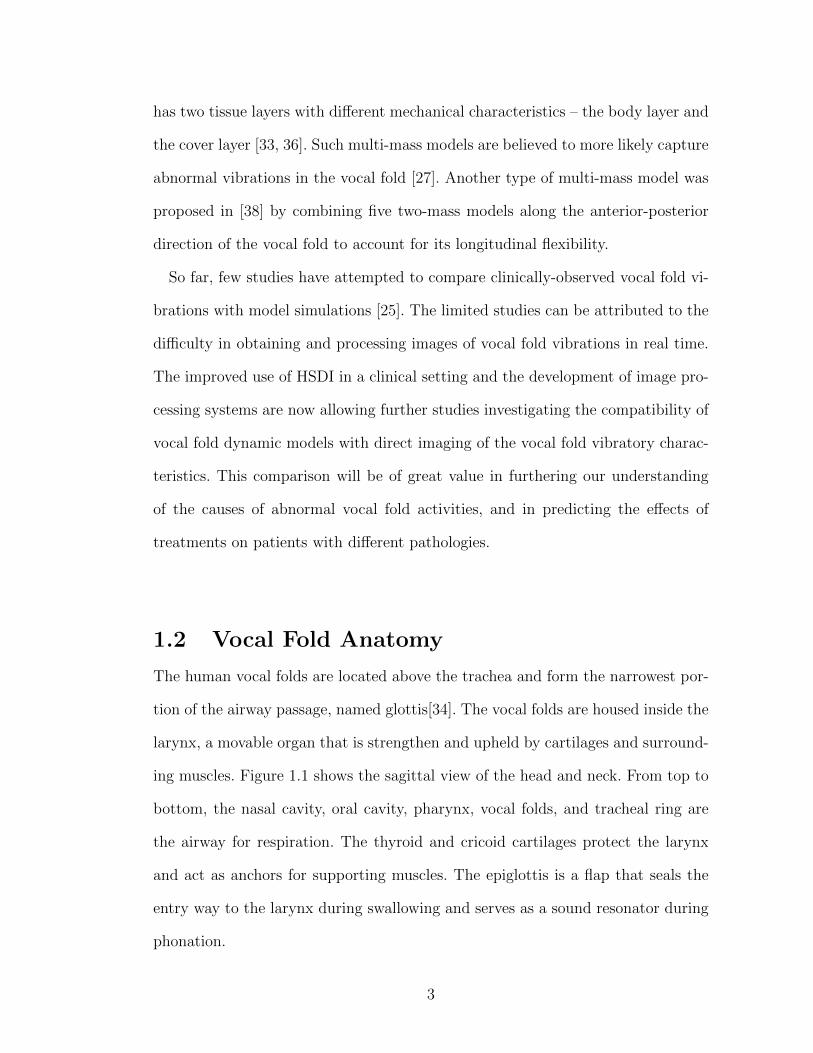
Each vocal fold is anteriorly and laterally attached to the thyroid cartilage, while
its posterior is connected to the anterior angle of the arytenoid cartilage (i.e., the
vocal process), as illustrated in Figure 1.2. The arytenoid cartilage, which sits on
the cricoid cartilage, has the freedom to rotate and slide, allowing the adduction
or abduction of the vocal folds by muscle activity. Specifically, the thyroarytenoid
muscle shortens and thickens the vocal folds by contraction [34]. The cricothyroid
muscle lengthens the vocal folds and is the primary pitch-control muscle. The
lateral cricoarytenoid muscle and the posterior cricoarytenoid muscle control the
4
Thyroid cartilage
Cricoid cartilage
Arytenoid cartilage
Vocal ligament
Glottis
Epiglottis
Corniculate cartilage
Cuneform cartilage
Ventricular fold
Vocal fold
Posterior
Anterior
Vocal process
Thyroarytenoid
Superior view ofsupporting ca tilagesr
Superior view ofocal foldv
FIGURE 1.2. Superior view of vocal folds. Left: supporting structure; right: superiorview.
vocal fold adduction and abduction, respectively. The interarytenoid muscle can
help narrow the posterior glottis.
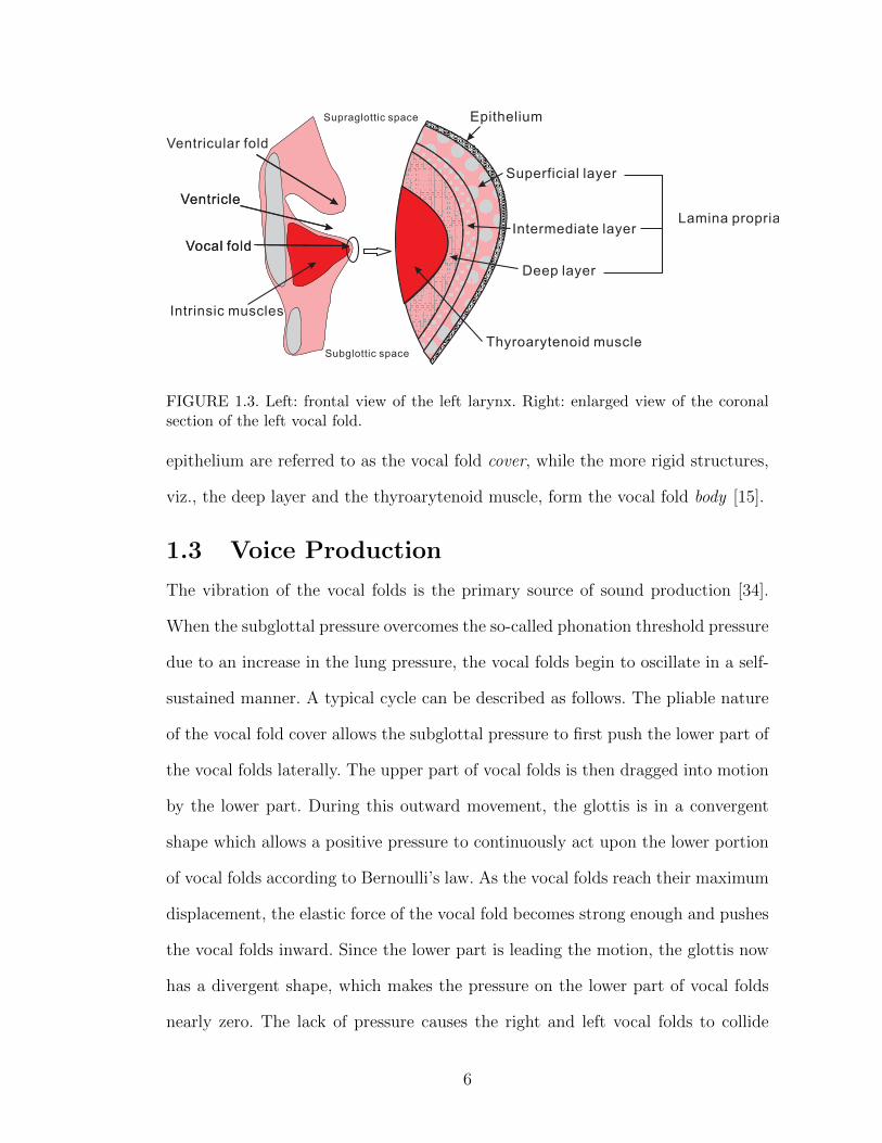
Histologically, the vocal folds are composed of three layered structures [13] as
shown in Figure 1.3: the epithelium, the lamina propria, and the thyroarytenoid
muscle. The lamina propria, which is made up of nonmuscular connective tissues, is
subdivided into three layers: superficial, intermediate, and deep layers. The super-
ficial layer is pliable with a loose fibrous structure that allows for large elongations.
The intermediate layer is composed of elastin fibers and collagen fibers along the
anterior and posterior directions [34]. The deep layer has more collagen fibers,
which provides more strength and rigidity. Due to the flexible nature of the su-
perficial and intermediate layers during phonation, these two layers together with
5
Ventricular fold
Vocal foldVocal fold
Intrinsic muscles
VentricleVentricle
Subglottic space
Supraglottic space Epithelium
Superficial layer
Intermediate layer
Deep layer
Thyroarytenoid muscle
Lamina propria
FIGURE 1.3. Left: frontal view of the left larynx. Right: enlarged view of the coronalsection of the left vocal fold.
epithelium are referred to as the vocal fold cover, while the more rigid structures,
viz., the deep layer and the thyroarytenoid muscle, form the vocal fold body [15].
1.3 Voice Production
The vibration of the vocal folds is the primary source of sound production [34].
When the subglottal pressure overcomes the so-called phonation threshold pressure
due to an increase in the lung pressure, the vocal folds begin to oscillate in a self-
sustained manner. A typical cycle can be described as follows. The pliable nature
of the vocal fold cover allows the subglottal pressure to first push the lower part of
the vocal folds laterally. The upper part of vocal folds is then dragged into motion
by the lower part. During this outward movement, the glottis is in a convergent
shape which allows a positive pressure to continuously act upon the lower portion
of vocal folds according to Bernoulli’s law. As the vocal folds reach their maximum
displacement, the elastic force of the vocal fold becomes strong enough and pushes
the vocal folds inward. Since the lower part is leading the motion, the glottis now
has a divergent shape, which makes the pressure on the lower part of vocal folds
nearly zero. The lack of pressure causes the right and left vocal folds to collide
6
with each other, closing the glottis. With the glottis closed, the pressure builds up
again and another cycle begins. It is this leading motion of the lower portion of
vocal folds, which is referred to as the “ribbon mode” or a “wave-like” movement
[34], that allows the subglottal pressure to transmit energy to the vocal folds and
sustain the vibration.
The vibrating vocal folds cause the air density near the outlet of the vocal folds
to cyclically increase and decrease (i.e., air condensation and rarefication). This
disturbance of the air density propagates back to the vocal trachea and forward
to the vocal tract. The vocal tract acts as a sound filter, amplifying selected fre-
quencies and suppressing others. Changes in the length and shape of the vocal
tract (e.g., tongue position and mouth shape) modulate the filter, modifying the
frequencies amplified/suppressed[34].
1.4 Voice Disorders
In this research, we will focus on characterizing the dynamics of three voice disor-
ders: vocal fold nodules, vocal fold polyp, and unilateral vocal fold paralysis.
Nodules are usually a benign lesion caused by the collision of the vocal folds
during phonation. As such, vocal nodules are symmetric and located in the middle
part of the vocal edges. Excessive collision of the vocal folds is believed to lead
to mechanical stresses [5, 34]. In the initial stage, when nodules first appear, they
are soft and pliable. If the abusive use of the vocal folds is prolonged, the edema
formed in early stages will undergo fibrosis and the nodules will harden and cause
hypertrophy of the epithelium. Acoustically, patients with nodules exhibit some
degree of dysphonia, jitter, and shimmer [5].
Polyp is usually caused by a localized irritation, such as smoke, chemicals, or
internal rupture of a blood vessel [34]. They are mainly unilateral. Compared
7
with nodules, polyps are typically larger, hemorrhagic, fibrotic, and inflammatory.
Acoustic signs of polyps and nodules are similar, however. Asymmetric motion of
the vocal folds can be observed by stroboscopy due to its unilateral occurrence [5].
Vocal fold paralysis is immobility of one or both vocal folds mostly caused by
lesions on the vagus nerve of the larynx (superior laryngeal nerve, recurrent la-
ryngeal nerve, or both). Clinical studies have found that unilateral paralysis is
more common than bilateral paralysis, accounting for 79.8% of paralysis cases [5].
Acoustically, patients with unilateral paralysis usually have breathy and hoarse
voice. Due to incomplete glottal closure, subglottal pressure and air flow are much
higher than normal [23].
1.5 Vocal Fold Examination
Vocal folds are usually examined via acoustical or imaging systems. With the
acoustical system, a variety of vocal fold characteristics can be obtained such as
fundamental frequency, phonation range, vocal intensity, and acoustic spectrum
[5]. The subject usually is instructed to produce simple vowels such as /ah/ or
/ee/, or a long reading or conversation. These acoustical signals are recorded by
microphone and simple digital data acquisition devices. Sound analysis software is
then applied to further manipulate the recorded signals.
Videostroboscopy uses a strobe to slow down the rapid vibrating vocal fold im-
age. However, this method has a capture rate of only 35 fps, which is not enough to
accurately examine the cycle of vibration. On the other hand, HSDI produces 2000
to 4000 fps and gives detailed phonation information. This technique first emerged
at the Bell Telephone Laboratories in 1937 [5], but only became affordable for
clinical application with the advent of high-speed digital cameras and digital data
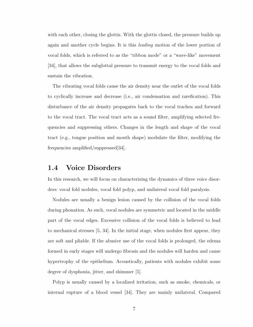
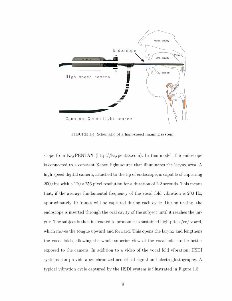
acquisition techniques. Figure 1.4 illustrates a HSDI system with a rigid endo-
8
Oral cavity
Nasal cavity
Tongue
Palate
Endoscope
High speed camera
Constant Xenon light source
FIGURE 1.4. Schematic of a high-speed imaging system.
scope from KayPENTAX (http://kaypentax.com). In this model, the endoscope
is connected to a constant Xenon light source that illuminates the larynx area. A
high-speed digital camera, attached to the tip of endoscope, is capable of capturing
2000 fps with a 120×256 pixel resolution for a duration of 2.2 seconds. This means
that, if the average fundamental frequency of the vocal fold vibration is 200 Hz,
approximately 10 frames will be captured during each cycle. During testing, the
endoscope is inserted through the oral cavity of the subject until it reaches the lar-
ynx. The subject is then instructed to pronounce a sustained high-pitch /ee/ vowel,
which moves the tongue upward and forward. This opens the larynx and lengthens
the vocal folds, allowing the whole superior view of the vocal folds to be better
exposed to the camera. In addition to a video of the vocal fold vibration, HSDI
systems can provide a synchronized acoustical signal and electroglottography. A
typical vibration cycle captured by the HSDI system is illustrated in Figure 1.5.
9
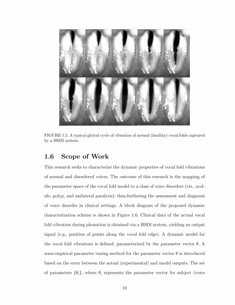
FIGURE 1.5. A typical glottal cycle of vibration of normal (healthy) vocal folds capturedby a HSDI system.
1.6 Scope of Work
This research seeks to characterize the dynamic properties of vocal fold vibrations
of normal and disordered voices. The outcome of this research is the mapping of
the parameter space of the vocal fold model to a class of voice disorders (viz., nod-
ule, polyp, and unilateral paralysis); thus,furthering the assessment and diagnosis
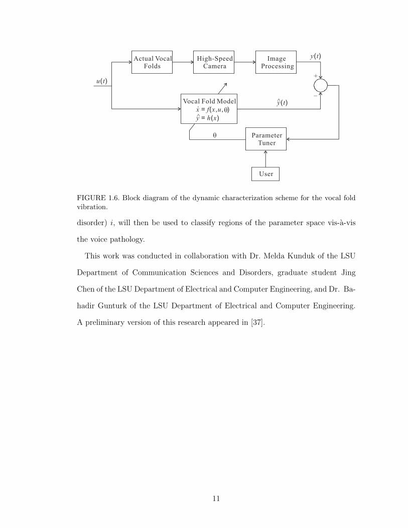
of voice disorder in clinical settings. A block diagram of the proposed dynamic
characterization scheme is shown in Figure 1.6. Clinical data of the actual vocal
fold vibration during phonation is obtained via a HSDI system, yielding an output
signal (e.g., position of points along the vocal fold edge). A dynamic model for
the vocal fold vibrations is defined, parameterized by the parameter vector θ. A
semi-empirical parameter tuning method for the parameter vector θ is introduced
based on the error between the actual (experimental) and model outputs. The set
of parameters {θi}, where θi represents the parameter vector for subject (voice
10
Actual VocalFolds
u t( )
Vocal Fold Model
x f x u= ( , , )q.
High-SpeedCamera
ImageProcessing
y t( )
+
_
y t( )^
ParameterTuner
q
User
y h x= ( )^
FIGURE 1.6. Block diagram of the dynamic characterization scheme for the vocal foldvibration.
disorder) i, will then be used to classify regions of the parameter space vis-a-vis
the voice pathology.
This work was conducted in collaboration with Dr. Melda Kunduk of the LSU
Department of Communication Sciences and Disorders, graduate student Jing
Chen of the LSU Department of Electrical and Computer Engineering, and Dr. Ba-
hadir Gunturk of the LSU Department of Electrical and Computer Engineering.
A preliminary version of this research appeared in [37].
11
Chapter 2Biomechanical Models of Vocal Folds
In this chapter, we provide a literature review of discrete (i.e., lumped-parameter)
vocal fold vibration modeling.
2.1 One-Mass Model
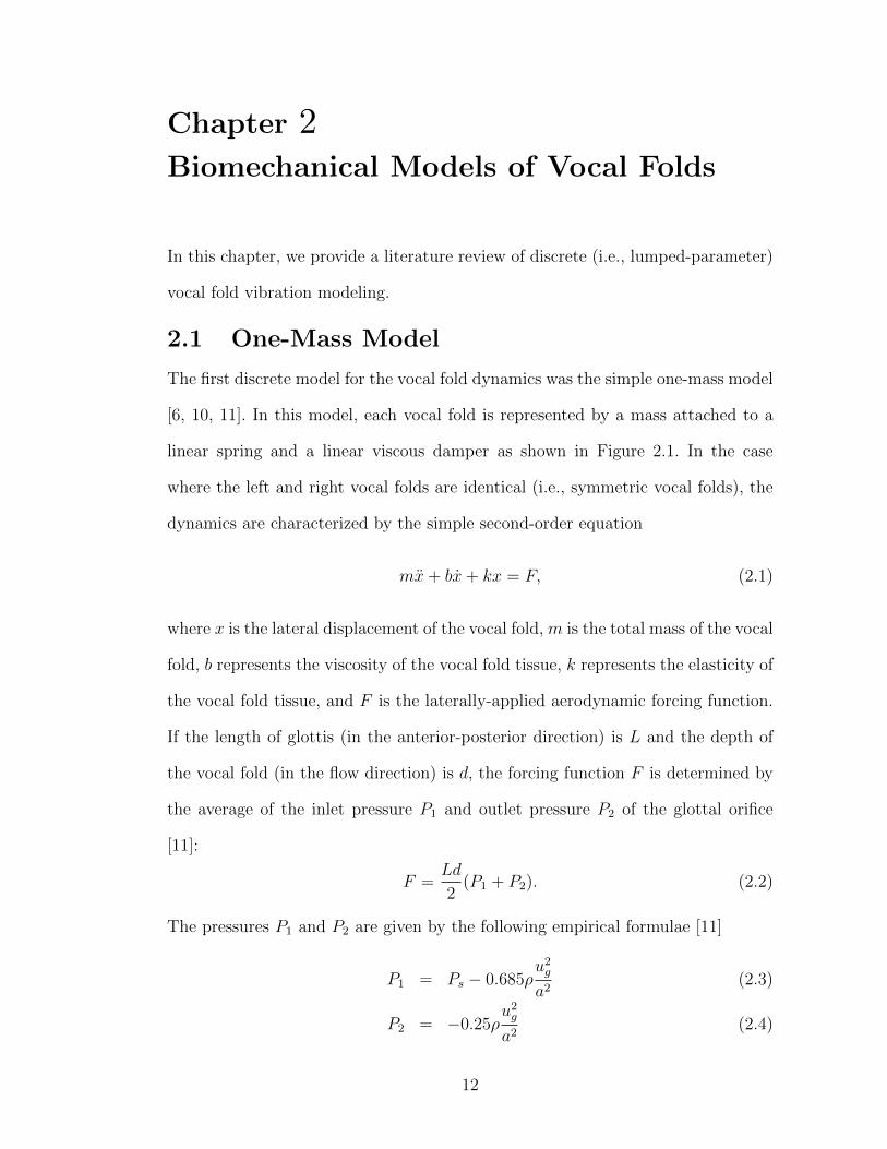
The first discrete model for the vocal fold dynamics was the simple one-mass model
[6, 10, 11]. In this model, each vocal fold is represented by a mass attached to a
linear spring and a linear viscous damper as shown in Figure 2.1. In the case
where the left and right vocal folds are identical (i.e., symmetric vocal folds), the
dynamics are characterized by the simple second-order equation
mx+ bx+ kx = F, (2.1)
where x is the lateral displacement of the vocal fold, m is the total mass of the vocal
fold, b represents the viscosity of the vocal fold tissue, k represents the elasticity of
the vocal fold tissue, and F is the laterally-applied aerodynamic forcing function.
If the length of glottis (in the anterior-posterior direction) is L and the depth of
the vocal fold (in the flow direction) is d, the forcing function F is determined by
the average of the inlet pressure P1 and outlet pressure P2 of the glottal orifice
[11]:
F =Ld
2(P1 + P2). (2.2)
The pressures P1 and P2 are given by the following empirical formulae [11]
P1 = Ps − 0.685ρu2ga2
(2.3)
P2 = −0.25ρu2ga2
(2.4)
12
Trachea
Vocal Tract
mm
kk
x
b
2 1/4"d
P2
P1
b
FIGURE 2.1. Schematic of the one-mass model.
where Ps is the subglottal pressure, ug is the volume flow rate in the glottis, ρ is
the air density, a = 2 (x+ x0)L is the glottal area, and x0 is the mass rest position.
The volume flow rate is a function of Ps and a, i.e., ug = ug(Ps, x), through the
coupling of (2.1) to the equations for the acoustic circuit of voice production; see
[11] for details.
Since the simple one-mass model assumes a uniform, one-dimensional motion for
the vocal fold layers, it does not accurately model most voice vibrations. Specifi-
cally, it is incapable of explaining how flow energy is transferred to the vocal folds
tissue to sustain the oscillation [34].
2.2 Two-Mass Model
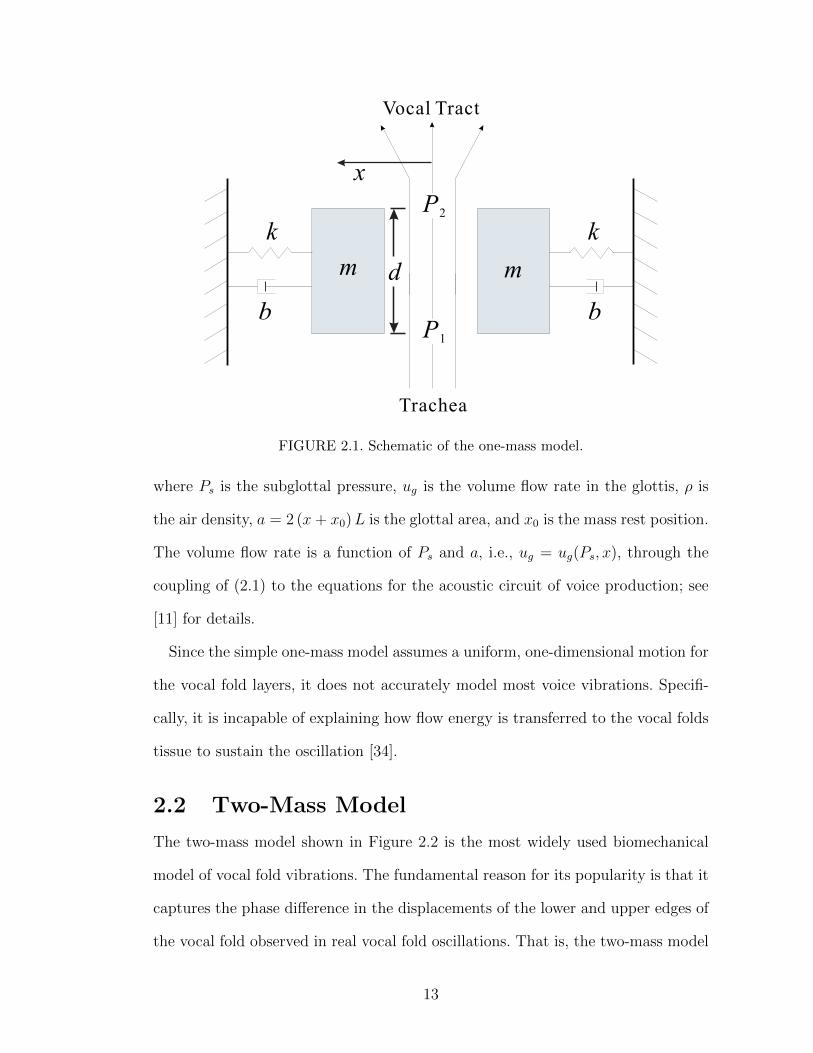
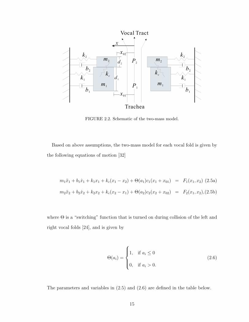
The two-mass model shown in Figure 2.2 is the most widely used biomechanical
model of vocal fold vibrations. The fundamental reason for its popularity is that it
captures the phase difference in the displacements of the lower and upper edges of
the vocal fold observed in real vocal fold oscillations. That is, the two-mass model
13
captures the fact that actual vocal folds have a wave-like motion from bottom to
top. This is illustrated in Figure 2.3, where we can see that the lower edge of the
vocal fold always leads the motion.
In the two-mass model, the masses do not strictly reflect the anatomical or phys-
iological structure of vocal folds, and are not directly related to vocal tissues [17].
The model assumes each vocal fold is represented by a pair of damped mechanical
oscillators coupled by a spring [17]. The glottis is approximated by rectangular
cross sections [2]. The two-mass model usually also includes the deformation of
the vocal folds during collision of the left/right folds. The two-mass model was
introduced in 1972 by [16] and later simplified in [32]. In original version of the
model, the mechanical and aerodynamical interactions were expressed as complex
coupled ordinary differential equations with many parameters [32]. The simplifying
assumptions are the following [7, 18, 32]:
• The cubic nonlinearity that models the elastic property of the vocal fold
tissue is neglected.
• The influence of tract and subglottal resonances is neglected.
• Subglottal and supraglottal resonances are negligible.
• The pressure drop at the inlet due to vena contracta is neglected.
• Viscous losses inside the glottis are neglected.
• The pressure force of the Bernoulli flow affects up to the narrowest part of
the glottis.
• The vocal folds are symmetric.
14
m2
kc
m1
k1
x
b2
b1
Trachea
Vocal Tract
k2
m1
m2
kc
k2
k1
b2
b1
P1
d1
x01
d2
P2
x02
FIGURE 2.2. Schematic of the two-mass model.
Based on above assumptions, the two-mass model for each vocal fold is given by
the following equations of motion [32]
m1x1 + b1x1 + k1x1 + kc(x1 − x2) + Θ(a1)c1(x1 + x01) = F1(x1, x2) (2.5a)
m2x2 + b2x2 + k2x2 + kc(x2 − x1) + Θ(a2)c2(x2 + x02) = F2(x1, x2),(2.5b)
where Θ is a “switching” function that is turned on during collision of the left and
right vocal folds [24], and is given by
Θ(ai) =
1, if ai ≤ 0
0, if ai > 0.
(2.6)
The parameters and variables in (2.5) and (2.6) are defined in the table below.
15
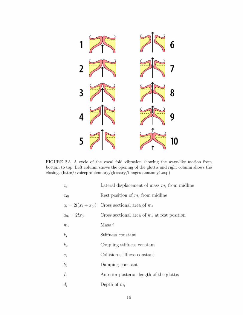
FIGURE 2.3. A cycle of the vocal fold vibration showing the wave-like motion frombottom to top. Left column shows the opening of the glottis and right column shows theclosing. (http://voiceproblem.org/glossary/images anatomy1.asp)
xi Lateral displacement of mass mi from midline
x0i Rest position of mi from midline
ai = 2l(xi + x0i) Cross sectional area of mi
a0i = 2lx0i Cross sectional area of mi at rest position
mi Mass i
ki Stiffness constant
kc Coupling stiffness constant
ci Collision stiffness constant
bi Damping constant
L Anterior-posterior length of the glottis
di Depth of mi
16
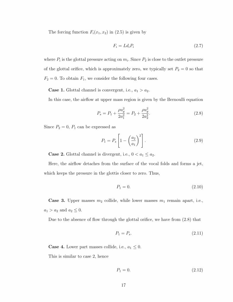
The forcing function Fi(x1, x2) in (2.5) is given by
Fi = LdiPi (2.7)
where Pi is the glottal pressure acting on mi. Since P2 is close to the outlet pressure
of the glottal orifice, which is approximately zero, we typically set P2 = 0 so that
F2 = 0. To obtain F1, we consider the following four cases.
Case 1. Glottal channel is convergent, i.e., a1 > a2.
In this case, the airflow at upper mass region is given by the Bernoulli equation
Ps = P1 +ρu2g2a21
= P2 +ρu2g2a22
. (2.8)
Since P2 = 0, P1 can be expressed as
P1 = Ps
[1−
(a2a1
)2]. (2.9)
Case 2. Glottal channel is divergent, i.e., 0 < a1 ≤ a2.
Here, the airflow detaches from the surface of the vocal folds and forms a jet,
which keeps the pressure in the glottis closer to zero. Thus,
P1 = 0. (2.10)
Case 3. Upper masses m2 collide, while lower masses m1 remain apart, i.e.,
a1 > a2 and a2 ≤ 0.
Due to the absence of flow through the glottal orifice, we have from (2.8) that
P1 = Ps. (2.11)
Case 4. Lower part masses collide, i.e., a1 ≤ 0.
This is similar to case 2, hence
P1 = 0. (2.12)
17
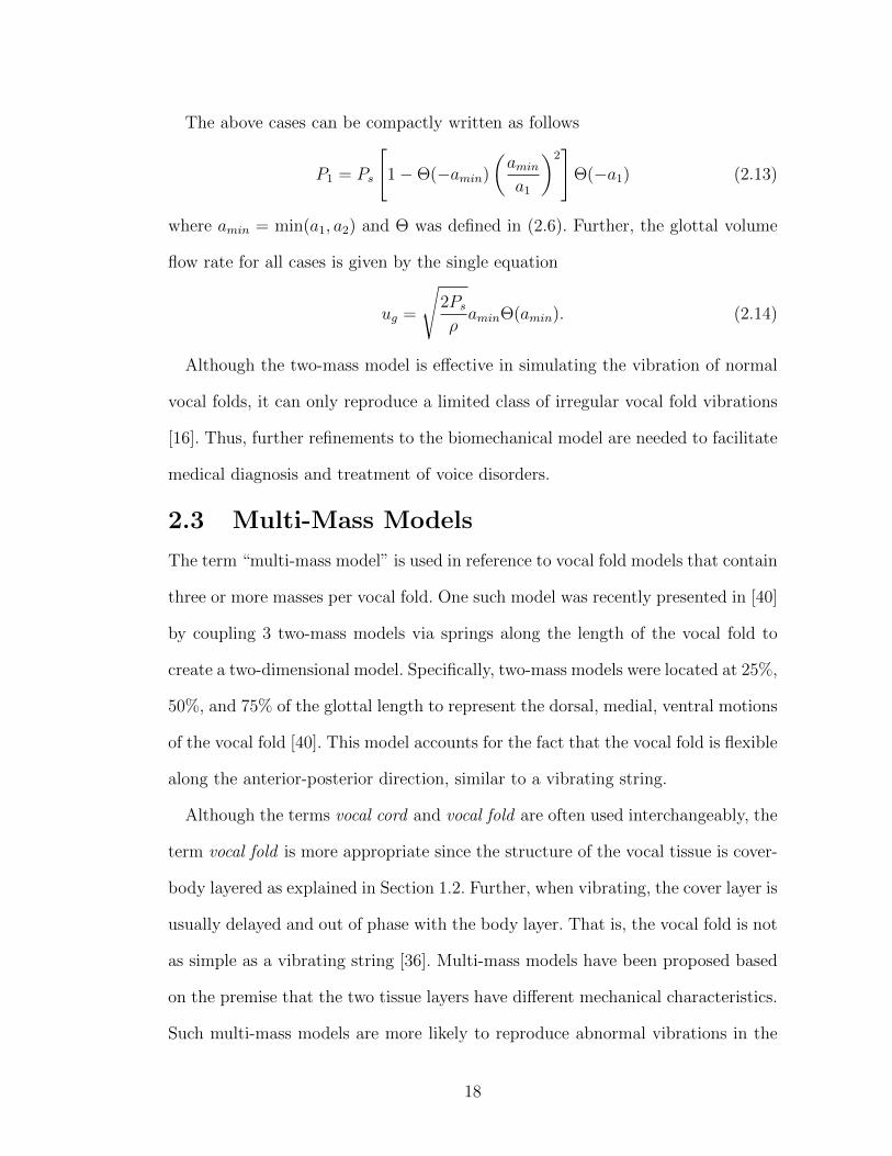
The above cases can be compactly written as follows
P1 = Ps
[1−Θ(−amin)
(amina1
)2]
Θ(−a1) (2.13)
where amin = min(a1, a2) and Θ was defined in (2.6). Further, the glottal volume
flow rate for all cases is given by the single equation
ug =
√2PsρaminΘ(amin). (2.14)
Although the two-mass model is effective in simulating the vibration of normal
vocal folds, it can only reproduce a limited class of irregular vocal fold vibrations
[16]. Thus, further refinements to the biomechanical model are needed to facilitate
medical diagnosis and treatment of voice disorders.
2.3 Multi-Mass Models
The term “multi-mass model” is used in reference to vocal fold models that contain
three or more masses per vocal fold. One such model was recently presented in [40]
by coupling 3 two-mass models via springs along the length of the vocal fold to
create a two-dimensional model. Specifically, two-mass models were located at 25%,
50%, and 75% of the glottal length to represent the dorsal, medial, ventral motions
of the vocal fold [40]. This model accounts for the fact that the vocal fold is flexible
along the anterior-posterior direction, similar to a vibrating string.
Although the terms vocal cord and vocal fold are often used interchangeably, the
term vocal fold is more appropriate since the structure of the vocal tissue is cover-
body layered as explained in Section 1.2. Further, when vibrating, the cover layer is
usually delayed and out of phase with the body layer. That is, the vocal fold is not
as simple as a vibrating string [36]. Multi-mass models have been proposed based
on the premise that the two tissue layers have different mechanical characteristics.
Such multi-mass models are more likely to reproduce abnormal vibrations in the
18
Trachea
Vocal tract
P2
k2
k3
b3
P1
b2
k1
b1
kc
m1
m2
m1
kc
m2
k2
k1
b1
k3
b3
b2
x
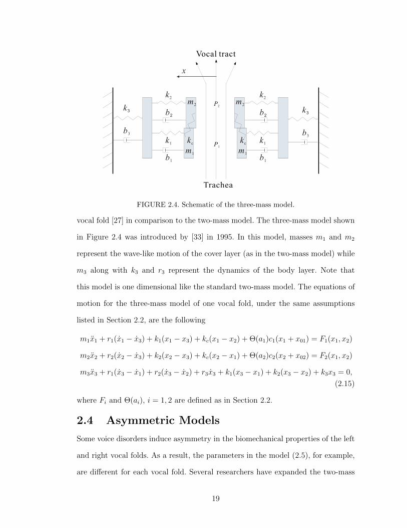
FIGURE 2.4. Schematic of the three-mass model.
vocal fold [27] in comparison to the two-mass model. The three-mass model shown
in Figure 2.4 was introduced by [33] in 1995. In this model, masses m1 and m2
represent the wave-like motion of the cover layer (as in the two-mass model) while
m3 along with k3 and r3 represent the dynamics of the body layer. Note that
this model is one dimensional like the standard two-mass model. The equations of
motion for the three-mass model of one vocal fold, under the same assumptions
listed in Section 2.2, are the following
m1x1 + r1(x1 − x3) + k1(x1 − x3) + kc(x1 − x2) + Θ(a1)c1(x1 + x01) = F1(x1, x2)
m2x2 + r2(x2 − x3) + k2(x2 − x3) + kc(x2 − x1) + Θ(a2)c2(x2 + x02) = F2(x1, x2)
m3x3 + r1(x3 − x1) + r2(x3 − x2) + r3x3 + k1(x3 − x1) + k2(x3 − x2) + k3x3 = 0,
(2.15)
where Fi and Θ(ai), i = 1, 2 are defined as in Section 2.2.
2.4 Asymmetric Models
Some voice disorders induce asymmetry in the biomechanical properties of the left
and right vocal folds. As a result, the parameters in the model (2.5), for example,
are different for each vocal fold. Several researchers have expanded the two-mass
19
model to study vibration with asymmetric variations in tension, resting glottal gap,
and subglottal pressure [17]. One asymmetric model is based on the asymmetry
factor Q defined as [8, 25]
kir = Qkil and mir =mil
Q, i = 1, 2. (2.16)
As the fundamental frequencies of the two-mass model oscillations can be approx-
imated by the simple mass-spring oscillator, it follows from (2.16) that
fr = Qfl (2.17)
where fr, fl are the vibration frequency of the right and left vocal folds, respectively.
For normal voices, it has been experimentally verified that 0.95 ≤ Q ≤ 1.05 for
females and 0.91 ≤ Q ≤ 1.10 for males [8]. That is, symmetry in the left/right
vocal fold vibrations (Q ≈ 1) is an important indicator of normal voice. Another
related approach for incorporating asymmetry into the two-mass model is to use
two asymmetry factors Qr and Ql defined as[7, 32]
kiα = Qαkiα0 and miα =miα0
Qα
, i = 1, 2; α = r, l (2.18)
where the subscript 0 denotes the standard parameter values. These so-called stan-
dard values are taken from the work in [16], which established relevant ranges for
the parameters of the two-mass model for normal voice. The fundamental frequen-
cies are then approximated as
fα = Qαfα0, α = r, l (2.19)
where fα0 is the “standard” vibration frequency of the α vocal fold [7, 32]. A
time-dependent version of (2.18) was discussed in [40].
A factor for quantifying the asymmetry between the anterior and posterior seg-
ments of a vocal fold, similar to (2.19), was introduced in [27]. In [39], factors were
proposed comprising both left/right and anterior/posterior asymmetries.
20
2.5 Estimation Approaches for Model
Parameters
An important topic of research in vocal fold modeling is identifying the model
parameters and correlating them with voice disorders. Here, we review previous
vocal fold modeling work where parameter estimation-like methods were used to
automatically identify the model parameters off-line.
In [7], a frequency-domain parameter estimation method was proposed to iden-
tify parameters of the two-mass model based on HSDI recordings of the vocal fold
vibrations. The time evolution of the distance between the medial position of the
left and right vocal folds were extracted from the model and HSDI recordings,
yielding theoretical and experimental curves, respectively. A nonconvex objective
function was defined as the difference between the dominant Fourier coefficients of
the theoretical and experimental curves, and the Nelder-Mead algorithm was used
for the minimization procedure. In [31], a Genetic Algorithm was used to identify
the subglottal pressure, masses, spring constants, and mass rest positions of the
multi-mass model proposed in [40]. The objective function was defined in the time
domain as a combination of two criteria that quantify the agreement between the
experimental and theoretical curves: the difference in glottal areas and the differ-
ence in distance of the dorsal, medial, and ventral vocal edges from the glottal axis.
In [39], the dynamics of the multi-mass model of [31] with time-varying parameters
were matched to vocal fold vibrations at the dorsal, medial, and ventral positions
using the discrete wavelet transform and Powell’s direct set method.
21
Chapter 3Proposed Biomechanical Model
In this chapter, we introduce a new, seven-mass biomechanical model for the vi-
bration of vocal folds. The model is based on the body-cover layer concept of the
vocal fold biomechanics, and segments the cover layer into three masses.
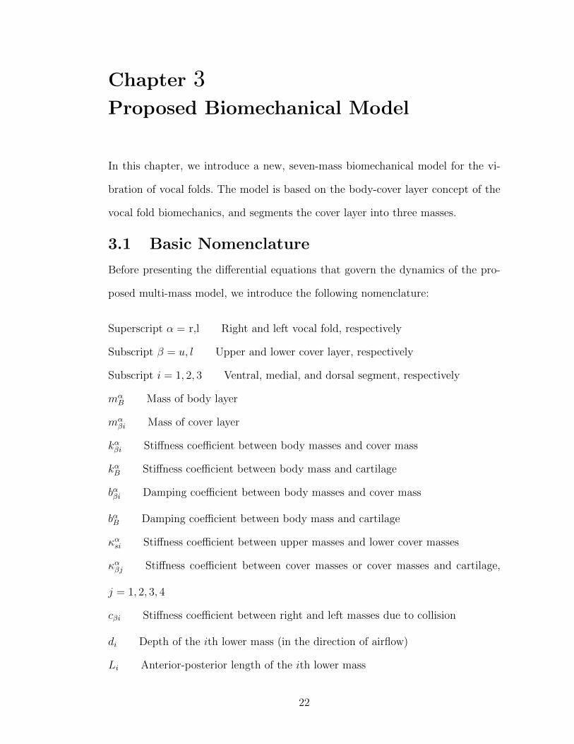
3.1 Basic Nomenclature
Before presenting the differential equations that govern the dynamics of the pro-
posed multi-mass model, we introduce the following nomenclature:
Superscript α = r,l Right and left vocal fold, respectively
Subscript β = u, l Upper and lower cover layer, respectively
Subscript i = 1, 2, 3 Ventral, medial, and dorsal segment, respectively
mαB Mass of body layer
mαβi Mass of cover layer
kαβi Stiffness coefficient between body masses and cover mass
kαB Stiffness coefficient between body mass and cartilage
bαβi Damping coefficient between body masses and cover mass
bαB Damping coefficient between body mass and cartilage
καsi Stiffness coefficient between upper masses and lower cover masses
καβj Stiffness coefficient between cover masses or cover masses and cartilage,
j = 1, 2, 3, 4
cβi Stiffness coefficient between right and left masses due to collision
di Depth of the ith lower mass (in the direction of airflow)
Li Anterior-posterior length of the ith lower mass
22
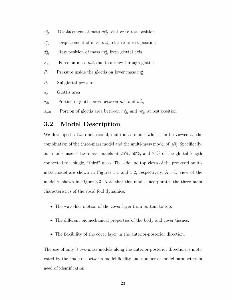
xαB Displacement of mass mαB relative to rest position
xαβi Displacement of mass mαβi relative to rest position
dαβi Rest position of mass mαβi from glottal axis
Fβi Force on mass mαβi due to airflow through glottis
Pi Pressure inside the glottis on lower mass mαli
Ps Subglottal pressure
aβ Glottis area
aβi Portion of glottis area between mrβi and ml
βi
aβi0 Portion of glottis area between mrβi and ml
βi at rest position
3.2 Model Description
We developed a two-dimensional, multi-mass model which can be viewed as the
combination of the three-mass model and the multi-mass model of [40]. Specifically,
our model uses 3 two-mass models at 25%, 50%, and 75% of the glottal length
connected to a single, “third” mass. The side and top views of the proposed multi-
mass model are shown in Figures 3.1 and 3.2, respectively. A 3-D view of the
model is shown in Figure 3.3. Note that this model incorporates the three main
characteristics of the vocal fold dynamics:
• The wave-like motion of the cover layer from bottom to top.
• The different biomechanical properties of the body and cover tissues.
• The flexibility of the cover layer in the anterior-posterior direction.
The use of only 3 two-mass models along the anterior-posterior direction is moti-
vated by the trade-off between model fidelity and number of model parameters in
need of identification.
23
Trachea
rm
ui
Vocal Tract
kui
mB
r
mli
r
kB
r
bB
r
r
bui
r
kli
r
bli
rk
si
r
lm
ui
kui
mB
l
mli
l
kB
l
bB
l
bui
kli
l
l
l
bli
lksi
l
Right Left
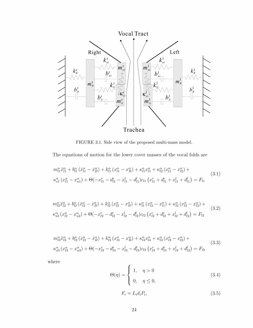
FIGURE 3.1. Side view of the proposed multi-mass model.
The equations of motion for the lower cover masses of the vocal folds are
mαl1x
αl1 + bαl1 (xαl1 − xαB) + kαl1 (xαl1 − xαB) + καl1x
αl1 + καl2 (xαl1 − xαl2) +
καs1 (xαl1 − xαu1) + Θ(−xrl1 − drl1 − xll1 − dll1)cl1(xrl1 + drl1 + xll1 + dll1
)= Fl1
(3.1)
mαl2x
αl2 + bαl2 (xαl2 − xαB) + kαl2 (xαl2 − xαB) + καl1 (xαl2 − xαl1) + καl2 (xαl2 − xαl3) +
καs2 (xαl2 − xαu2) + Θ(−xrl2 − drl2 − xll2 − dll2)cl2(xrl2 + drl2 + xll2 + dll2
)= Fl2
(3.2)
mαl3x
αl3 + bαl3 (xαl3 − xαB) + kαl3 (xαl3 − xαB) + καl4x
αl4 + καl3 (xαl3 − xαl2) +
καs3 (xαl3 − xαu3) + Θ(−xrl3 − drl3 − xll3 − dll3)cl3(xrl3 + drl3 + xll3 + dll3
)= Fl3
(3.3)
where
Θ(η) =
1, η > 0
0, η ≤ 0,(3.4)
Fi = LidiPi, (3.5)
24
Anterior
Posterior
mB
r
kB
r
bB
r
ku1
r
bu1
r
ku2
r
bu2
r
ku3r
bu3
r
ku1
r
rm
u1
rm
u2
rm
u3
ku2
r
ku4
r
mB
l
kB
l
bB
l
ku1
l
bu1
l
ku2l
bu2
l
ku3l
bu3
l
ku1
l
lm
u1
lm
u2
lmu3
ku2l
ku4l
ku3
rk
u3l
Dorsal
Ventral
Medial
Right Left
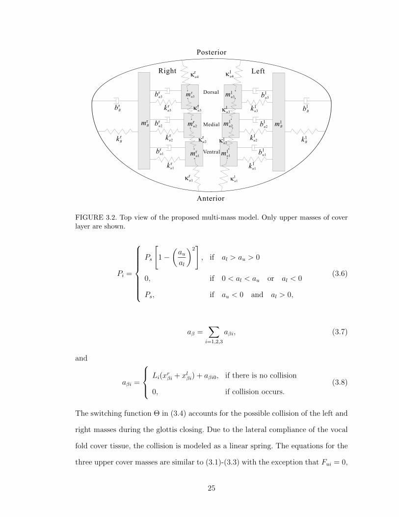
FIGURE 3.2. Top view of the proposed multi-mass model. Only upper masses of coverlayer are shown.
Pi =
Ps
[1−
(aual
)2], if al > au > 0
0, if 0 < al < au or al < 0
Ps, if au < 0 and al > 0,
(3.6)
aβ =∑i=1,2,3
aβi, (3.7)
and
aβi =
Li(xrβi + xlβi) + aβi0, if there is no collision
0, if collision occurs.(3.8)
The switching function Θ in (3.4) accounts for the possible collision of the left and
right masses during the glottis closing. Due to the lateral compliance of the vocal
fold cover tissue, the collision is modeled as a linear spring. The equations for the
three upper cover masses are similar to (3.1)-(3.3) with the exception that Fui = 0,
25
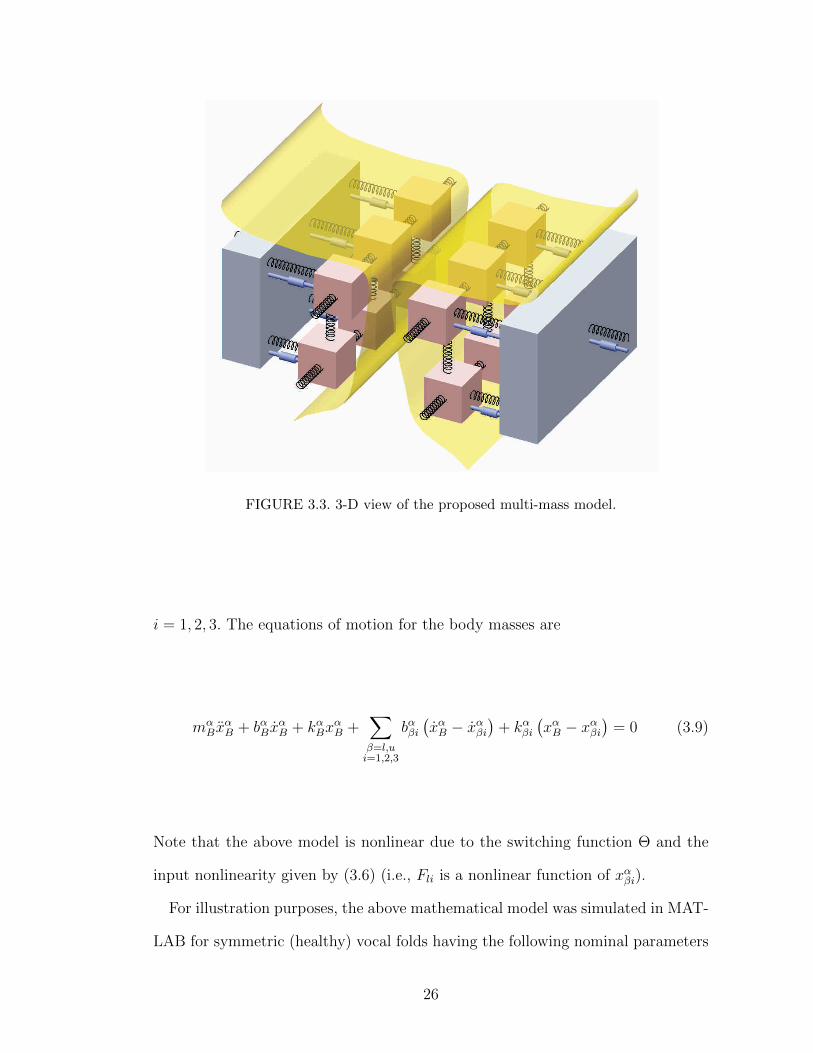
FIGURE 3.3. 3-D view of the proposed multi-mass model.
i = 1, 2, 3. The equations of motion for the body masses are
mαBx
αB + bαBx
αB + kαBx
αB +
∑β=l,ui=1,2,3
bαβi(xαB − xαβi
)+ kαβi
(xαB − xαβi
)= 0 (3.9)
Note that the above model is nonlinear due to the switching function Θ and the
input nonlinearity given by (3.6) (i.e., Fli is a nonlinear function of xαβi).
For illustration purposes, the above mathematical model was simulated in MAT-
LAB for symmetric (healthy) vocal folds having the following nominal parameters
26
[33]
mαB = 0.05 g, mα
βi = 0.0033 g,
kαli = 0.0017 g/ms2, kαui = 0.0012 g/ms2, kαB = 0.1 g/ms2,
bαli = 1.9× 10⁻³ g/ms, bαui = 1.6× 10⁻³ g/ms, bαB = 0.0283 g/ms,
καsi = 0.00067 g/ms2, καli = 0.0083 g/ms2,
καui = 0.0058 g/ms2, cβi = 3kαβi,
Li = 0.4 cm, wi = 0.15 cm,
dαl1 = 0.0045 cm, dαl2 = 0.018 cm, dαl3 = 0.032 cm,
dαu1 = 0.00447 cm, dαu2 = 0.0179 cm, dαu3 = 0.0313 cm,
Ps = 0.008 g/(cm-ms2).
(3.10)
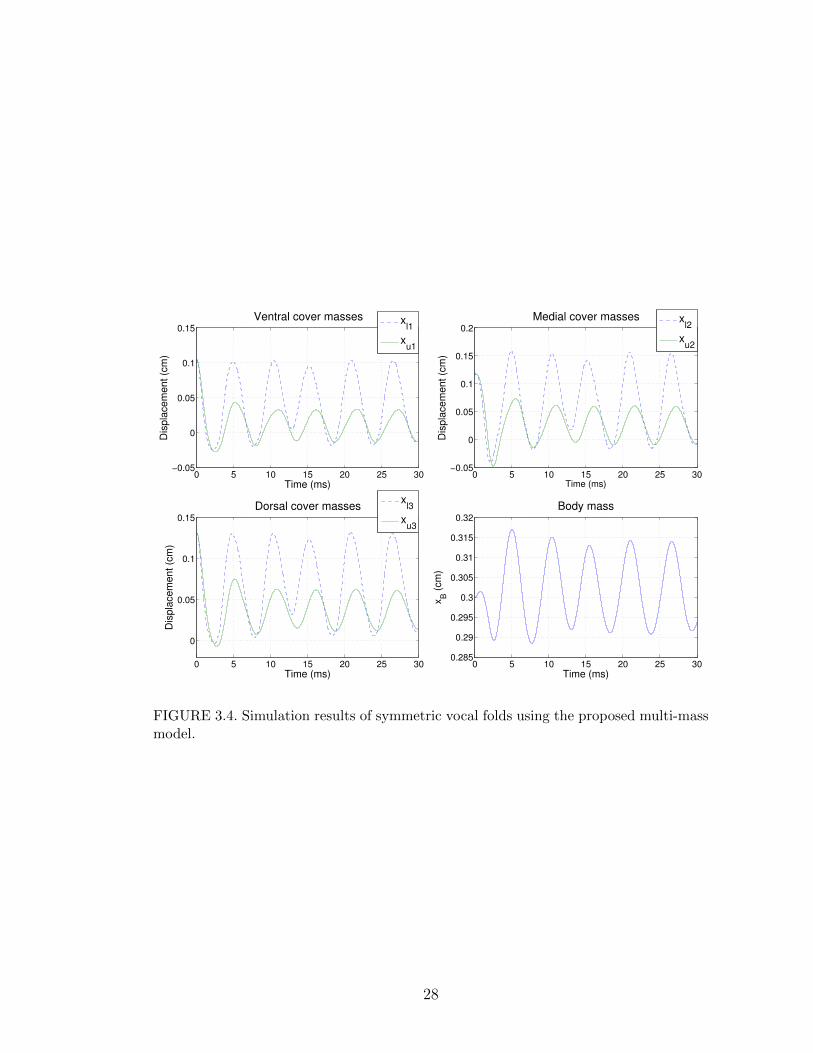
All the initial conditions were set to zero, except for xαβi = 0.1 cm. The simulation
results for the displacements of the seven masses are shown in Figure 3.4. Due
to the symmetry of the simulated vocal folds, only the vibrations of one side are
shown. Notice how the lower masses always lead the motion relative to the upper
masses, as expected.
27
0 5 10 15 20 25 30−0.05
0
0.05
0.1
0.15
Ventral cover masses
Dis
pla
cem
ent (c
m)
Time (ms)
x
l1
xu1
0 5 10 15 20 25 30−0.05
0
0.05
0.1
0.15
0.2
Medial cover masses
Dis
pla
cem
ent (c
m)
Time (ms)
xl2
xu2
0 5 10 15 20 25 30
0
0.05
0.1
0.15
Dorsal cover masses
Dis
pla
cem
ent (c
m)
Time (ms)
xl3
xu3
0 5 10 15 20 25 300.285
0.29
0.295
0.3
0.305
0.31
0.315
0.32
Body mass
xB (
cm
)
Time (ms)
FIGURE 3.4. Simulation results of symmetric vocal folds using the proposed multi-massmodel.
28
Chapter 4Tuning of Model Parameters
In order to validate the biomechanical model given by (3.1)-(3.9), we will evalu-
ate its ability to reproduce actual vibrations of healthy and pathological (nodule,
polyp, and unilateral paralysis) vocal folds by comparing the model response to
experimental data obtained from a HSDI system. The model parameters (viz.,
masses, stiffnesses, damping coefficients, mass rest positions, and subglottal pres-
sure) directly influence the model response. Therefore, in this chapter, we will
introduce semi-empirical procedures for tuning the parameters so that the model
response matches as closely as possible experimental data from given vocal folds.
Specifically, we seek to match the displacement in time and fast Fourier transform
(FFT) data of the ventral, medial, and dorsal segments of the vocal fold edges.
We present a two-stage parameter tuning approach. The first stage involves the
manual coarse tuning of parameters based on a data set consisting of 90 ms of
simulation time, 64 ms of experimental time, and a 128-point FFT for both the
simulation and experimental data. These values were used to expedite the manual
course-tuning process. This tuning stage is initialized with a nominal parameter
set for healthy vocal folds, viz., the parameter set in (3.10). At the end of this
stage, we obtain a model parameter set whose responses are relatively close to
their experimental counterparts. Since the 128-point FFT is not very accurate, we
then run an automatic fine-tuning process on a subset of the parameters tuned in
stage one using 280 ms of simulation time, 256 ms of experimental time, and a
512-point FFT.
29
Due to the inability of the HSDI system to distinguish the lower and upper edges
of the vocal fold (see Section 5.1), the model simulation needs to mimic this fact
to enable a proper comparison with the experimental data. To this end, we obtain
the contour of the vocal folds in the simulation by setting the left and right vocal
fold edges to
xαi :=
min(xαli + dαli, x
αui + dαui), if section i of glottis is open
Position of the collision, if collision occurs in section i.
(4.1)
Thus, we use the vocal fold segment variables xαi to compare the model simulation
with the experimental data.
4.1 Manual Coarse-Tuning Procedure
To reduce the number of parameters to be tuned, the damping coefficients bαβi and
bαB in the model were set to [33]
bαβi = 2ζ1√mαβik
αβi (4.2)
and
bαB = 2ζ2√mαBk
αB (4.3)
where the damping ratio ζ1 is set to a value in the interval [0.3, 0.4] if there is no
collision and to a value in the interval [0.6, 0.8] if collision occurs, and
ζ2 = 0.4. (4.4)
The manual tuning of the model parameters begins with an initial, standard
parameter set; e.g., the parameter set in (3.10). For each change of parameters, the
simulation outputs the FFT and time domain behavior of xαi . The tuning of each
parameter from its initial value is guided by the following physical observations
and insights.
30
• The fundamental frequency of the steady-state vibrations of (3.1)-(3.9) is
partially dependent on the fundamental frequency of the Bernoulli pressure
Pi. However, the Bernoulli pressure depends on the relative displacement of
upper and lower masses (see (3.6)-(3.8)), complicating the determination of
its fundamental frequency. Fortunately, we observed after running several
simulations with different parameter values that the fundamental frequency
of the steady-state vibrations is very close to the one for the unforced system,
which is obtained by setting Fli = 0 in (3.1)-(3.3). This observation facilitates
the parameter tuning since we can assume that the vibration frequencies are
proportional to√k/m where k is the spring constant and m is the mass.
• The amplitude of the vocal fold vibration is mostly sensitive to the tension
of the vocal folds close to the edge and to the subglottal pressure. Increasing
the subglottal pressure increases the amplitude, while increasing the tension
decreases the amplitude. Since only lateral motions are considered in the
proposed model, the vocal fold tension is represented by the spring constants
καβi.
• Asymmetric configuration of masses causes phase differences between left
and right displacement. The side with lighter mass will lead the side with
heavier mass.
• The collision of the vocal folds is mostly affected by the collision springs cβi,
the stiffness coupling the upper and lower masses καsi, and the rest position
of the masses dαβi.
Based on the above facts, the manual coarse tuning of the model parameters
was conducted according to the following procedure:
31
1. Tune mαβi, k
αβi, and καβi until the frequency of the first harmonic in the FFT
of xαi roughly (visually) matches the corresponding experimental value.
2. Tune kαβi, καβi and Ps until the amplitude of the first harmonic in the FFT of
xαi roughly matches the corresponding experimental value. If the frequencies
of the first harmonic shift as a result, go back to step 1.
3. Tune καsi, cβi, and dαβi until the duration of collisions and the vibration am-
plitudes of xαi in time roughly match the corresponding experimental value.
If the frequencies of the first harmonic shift as a result, go back to step 1.
4. Tune mαβi until phase difference between xri and xli in time roughly matches
the corresponding experimental value. If the frequencies of the first harmonic
shift as a result, go back to step 1.
4.2 Automatic Fine-Tuning Procedure
In this tuning stage, we introduce some variables to make the comparison between
the model and experimental data more objective and to automate the tuning pro-
cess. To this end, we define
f =
∑α
∑i
[fα0i]exp − [fα0i]model
6(4.5)
where fα0i is the fundamental frequency (first harmonic) of the FFT of xαi . Let xαi (j)
and xαi (j) be the maximum and minimum displacement of xαi in cycle j, respec-
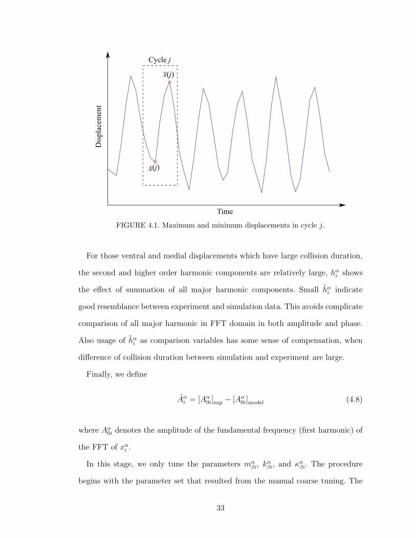
tively, as shown in Figure 4.1. The average peak-to-peak displacement amplitude
is defined as
hαi =1
Nc
Nc∑j=1
[xαi (j)− xαi (j)] (4.6)
where Nc is number of cycles in the data set. The error in hαi is then given by
hαi = [hαi ]exp − [hαi ]model . (4.7)
32
Cycle j
Dis
pla
cem
ent
Time
x j( )
x j( )
FIGURE 4.1. Maximum and minimum displacements in cycle j.
For those ventral and medial displacements which have large collision duration,
the second and higher order harmonic components are relatively large, hαi shows
the effect of summation of all major harmonic components. Small hαi indicate
good resemblance between experiment and simulation data. This avoids complicate
comparison of all major harmonic in FFT domain in both amplitude and phase.
Also usage of hαi as comparison variables has some sense of compensation, when
difference of collision duration between simulation and experiment are large.
Finally, we define
Aαi = [Aα0i]exp − [Aα0i]model (4.8)
where Aα0i denotes the amplitude of the fundamental frequency (first harmonic) of
the FFT of xαi .
In this stage, we only tune the parameters mαβi, k
αβi, and καβi. The procedure
begins with the parameter set that resulted from the manual coarse tuning. The
33
Start
Update ρ
Fine-tuned parameter set
Y
Y
N
N
f < ?e f
~ ρα
m , ,βiβi
ρk
α
βiκα
ρβi
h
A
a
a
<
<
and
e
e
hi
Ai
~i
a
i
~a
Update sa s [
a αm , , ]βik
α
βiκα
βi
Run modelsimulation
FIGURE 4.2. Flowchart of fine tuning procedure.
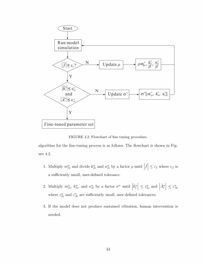
algorithm for the fine-tuning process is as follows. The flowchart is shown in Fig-
ure 4.2.
1. Multiply mαβi and divide kαβi and καβi by a factor ρ until
∣∣∣f ∣∣∣ ≤ εf where εf is
a sufficiently small, user-defined tolerance.
2. Multiply mαβi, k
αβi, and καβi by a factor σα until
∣∣∣hαi ∣∣∣ ≤ εαhi and∣∣∣Aαi ∣∣∣ ≤ εαAi
where εαhi and εαAi are sufficiently small, user-defined tolerances.
3. If the model does not produce sustained vibration, human intervention is
needed.
34
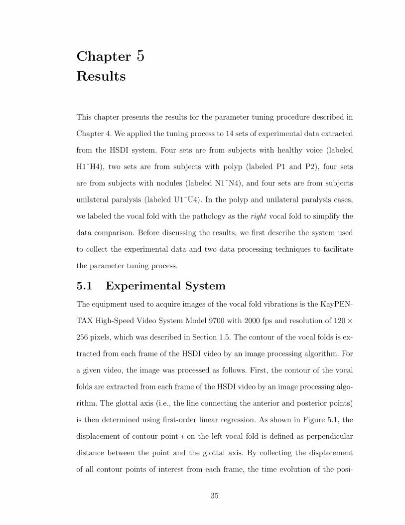
Chapter 5Results
This chapter presents the results for the parameter tuning procedure described in
Chapter 4. We applied the tuning process to 14 sets of experimental data extracted
from the HSDI system. Four sets are from subjects with healthy voice (labeled
H1˜H4), two sets are from subjects with polyp (labeled P1 and P2), four sets
are from subjects with nodules (labeled N1˜N4), and four sets are from subjects
unilateral paralysis (labeled U1˜U4). In the polyp and unilateral paralysis cases,
we labeled the vocal fold with the pathology as the right vocal fold to simplify the
data comparison. Before discussing the results, we first describe the system used
to collect the experimental data and two data processing techniques to facilitate
the parameter tuning process.
5.1 Experimental System
The equipment used to acquire images of the vocal fold vibrations is the KayPEN-
TAX High-Speed Video System Model 9700 with 2000 fps and resolution of 120×
256 pixels, which was described in Section 1.5. The contour of the vocal folds is ex-
tracted from each frame of the HSDI video by an image processing algorithm. For
a given video, the image was processed as follows. First, the contour of the vocal
folds are extracted from each frame of the HSDI video by an image processing algo-
rithm. The glottal axis (i.e., the line connecting the anterior and posterior points)
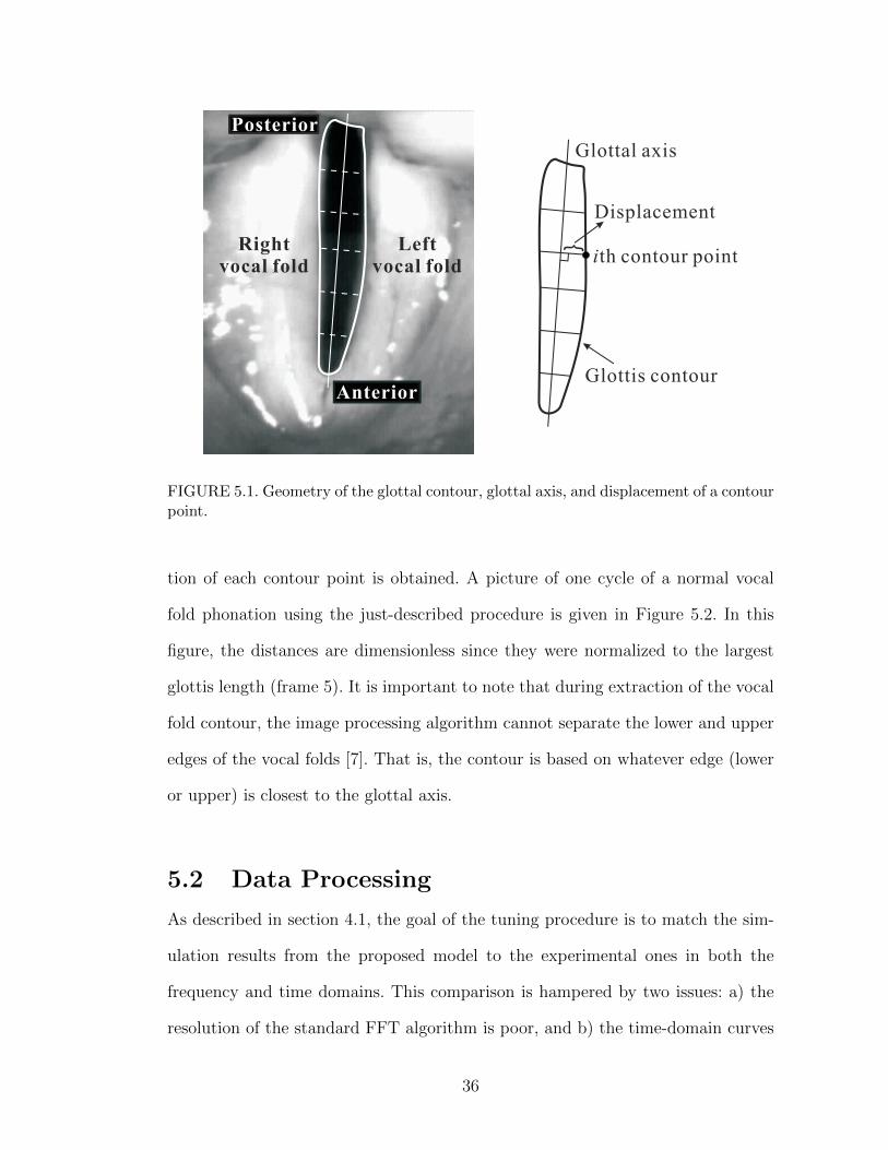
is then determined using first-order linear regression. As shown in Figure 5.1, the
displacement of contour point i on the left vocal fold is defined as perpendicular
distance between the point and the glottal axis. By collecting the displacement
of all contour points of interest from each frame, the time evolution of the posi-
35
Glottis contour
Leftvocal fold
Posterior
Anterior
Rightvocal fold
Glottal axis
Displacement
ith contour point
FIGURE 5.1. Geometry of the glottal contour, glottal axis, and displacement of a contourpoint.
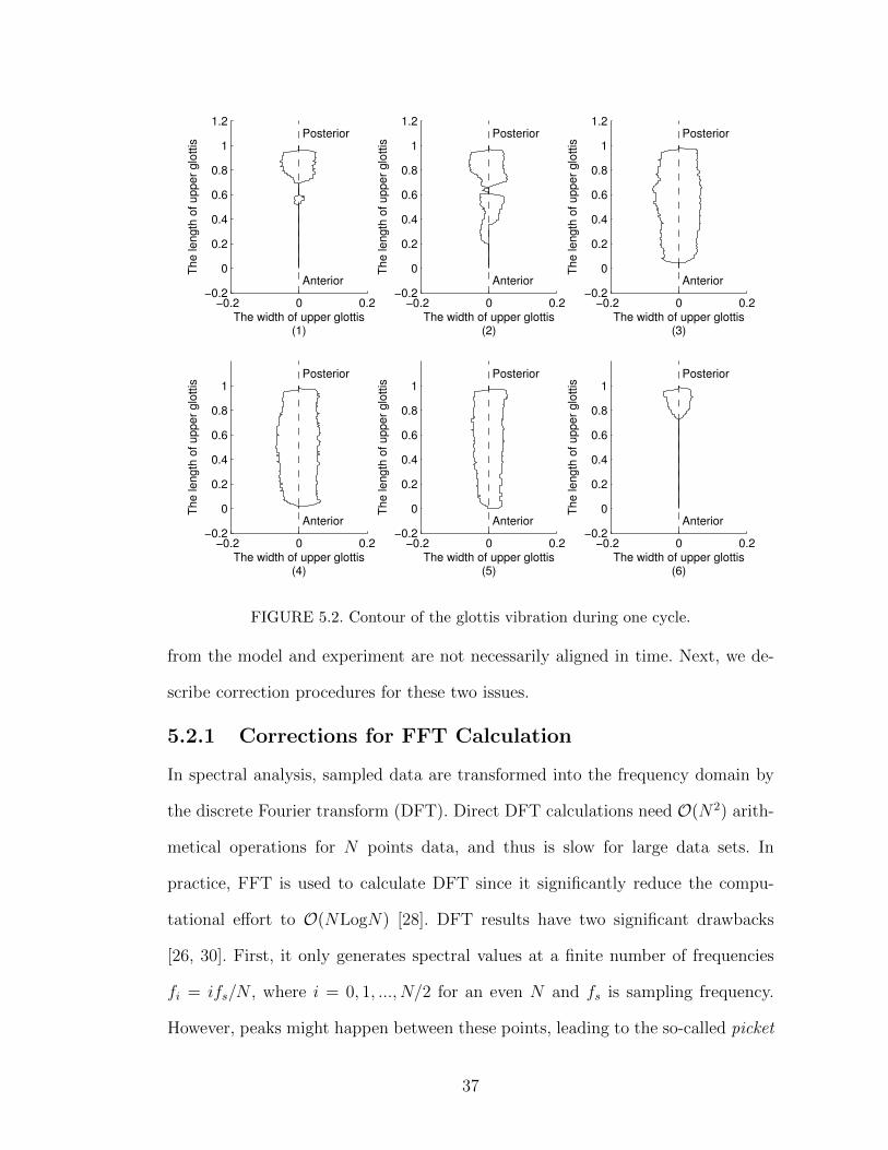
tion of each contour point is obtained. A picture of one cycle of a normal vocal
fold phonation using the just-described procedure is given in Figure 5.2. In this
figure, the distances are dimensionless since they were normalized to the largest
glottis length (frame 5). It is important to note that during extraction of the vocal
fold contour, the image processing algorithm cannot separate the lower and upper
edges of the vocal folds [7]. That is, the contour is based on whatever edge (lower
or upper) is closest to the glottal axis.
5.2 Data Processing
As described in section 4.1, the goal of the tuning procedure is to match the sim-
ulation results from the proposed model to the experimental ones in both the
frequency and time domains. This comparison is hampered by two issues: a) the
resolution of the standard FFT algorithm is poor, and b) the time-domain curves
36
−0.2 0 0.2−0.2
0
0.2
0.4
0.6
0.8
1
1.2
The width of upper glottis(1)
Th
e le
ng
th o
f u
pp
er
glo
ttis
Posterior
Anterior
−0.2 0 0.2−0.2
0
0.2
0.4
0.6
0.8
1
1.2
The width of upper glottis(2)
Th
e le
ng
th o
f u
pp
er
glo
ttis
Posterior
Anterior
−0.2 0 0.2−0.2
0
0.2
0.4
0.6
0.8
1
1.2
The width of upper glottis(3)
Th
e le
ng
th o
f u
pp
er
glo
ttis
Posterior
Anterior
−0.2 0 0.2−0.2
0
0.2
0.4
0.6
0.8
1
The width of upper glottis(4)
Th
e le
ng
th o
f u
pp
er
glo
ttis
Posterior
Anterior
−0.2 0 0.2−0.2
0
0.2
0.4
0.6
0.8
1
The width of upper glottis(5)
Th
e le
ng
th o
f u
pp
er
glo
ttis
Posterior
Anterior
−0.2 0 0.2−0.2
0
0.2
0.4
0.6
0.8
1
The width of upper glottis(6)
Th
e le
ng
th o
f u
pp
er
glo
ttis
Posterior
Anterior
FIGURE 5.2. Contour of the glottis vibration during one cycle.
from the model and experiment are not necessarily aligned in time. Next, we de-
scribe correction procedures for these two issues.
5.2.1 Corrections for FFT Calculation
In spectral analysis, sampled data are transformed into the frequency domain by
the discrete Fourier transform (DFT). Direct DFT calculations need O(N2) arith-
metical operations for N points data, and thus is slow for large data sets. In
practice, FFT is used to calculate DFT since it significantly reduce the compu-
tational effort to O(NLogN) [28]. DFT results have two significant drawbacks
[26, 30]. First, it only generates spectral values at a finite number of frequencies
fi = ifs/N , where i = 0, 1, ..., N/2 for an even N and fs is sampling frequency.
However, peaks might happen between these points, leading to the so-called picket
37
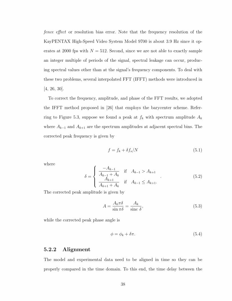
fence effect or resolution bias error. Note that the frequency resolution of the
KayPENTAX High-Speed Video System Model 9700 is about 3.9 Hz since it op-
erates at 2000 fps with N = 512. Second, since we are not able to exactly sample
an integer multiple of periods of the signal, spectral leakage can occur, produc-
ing spectral values other than at the signal’s frequency components. To deal with
these two problems, several interpolated FFT (IFFT) methods were introduced in
[4, 26, 30].
To correct the frequency, amplitude, and phase of the FFT results, we adopted
the IFFT method proposed in [26] that employs the barycenter scheme. Refer-
ring to Figure 5.3, suppose we found a peak at fk with spectrum amplitude Ak
where Ak−1 and Ak+1 are the spectrum amplitudes at adjacent spectral bins. The
corrected peak frequency is given by
f = fk + δfs/N (5.1)
where
δ =
−Ak−1
Ak−1 + Akif Ak−1 > Ak+1
Ak+1
Ak+1 + Akif Ak−1 ≤ Ak+1.
. (5.2)
The corrected peak amplitude is given by
A =Akπδ
sin πδ=
Aksinc δ
, (5.3)
while the corrected peak phase angle is
φ = φk + δπ. (5.4)
5.2.2 Alignment
The model and experimental data need to be aligned in time so they can be
properly compared in the time domain. To this end, the time delay between the
38
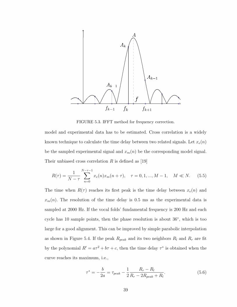
FIGURE 5.3. IFFT method for frequency correction.
model and experimental data has to be estimated. Cross correlation is a widely
known technique to calculate the time delay between two related signals. Let xe(n)
be the sampled experimental signal and xm(n) be the corresponding model signal.
Their unbiased cross correlation R is defined as [19]
R(τ) =1
N − τ
N−τ−1∑n=0
xe(n)xm(n+ τ), τ = 0, 1, ...,M − 1, M � N. (5.5)
The time when R(τ) reaches its first peak is the time delay between xe(n) and
xm(n). The resolution of the time delay is 0.5 ms as the experimental data is
sampled at 2000 Hz. If the vocal folds’ fundamental frequency is 200 Hz and each
cycle has 10 sample points, then the phase resolution is about 36◦, which is too
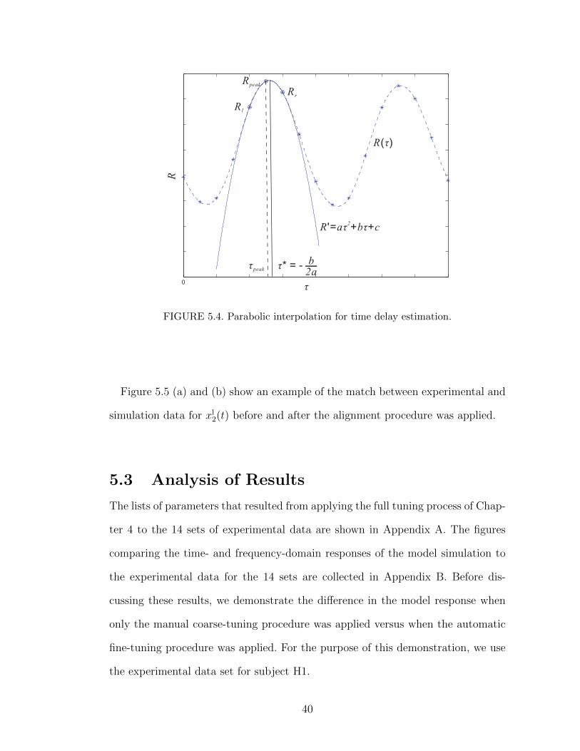
large for a good alignment. This can be improved by simple parabolic interpolation
as shown in Figure 5.4. If the peak Rpeak and its two neighbors Rl and Rr are fit
by the polynomial R′ = aτ 2 + bτ + c, then the time delay τ ∗ is obtained when the
curve reaches its maximum, i.e.,
τ ∗ = − b
2a= τpeak −
1
2
Rr −Rl
Rr − 2Rpeak +Rl
. (5.6)
39
0
R
R l
Rr
Rpeak
R( )τ
R a b c'= + +τ τ2
τpeak τ* = -b
2a
τ
FIGURE 5.4. Parabolic interpolation for time delay estimation.
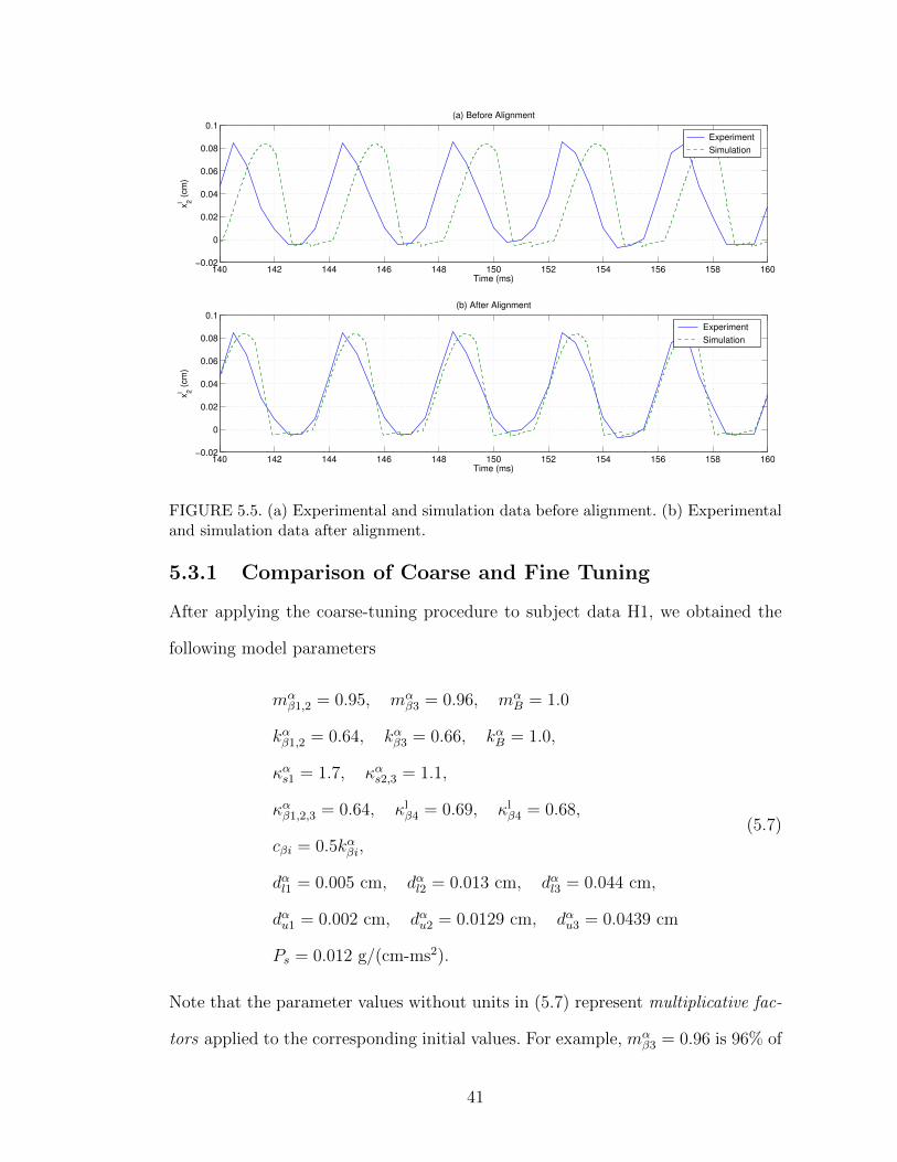
Figure 5.5 (a) and (b) show an example of the match between experimental and
simulation data for xl2(t) before and after the alignment procedure was applied.
5.3 Analysis of Results
The lists of parameters that resulted from applying the full tuning process of Chap-
ter 4 to the 14 sets of experimental data are shown in Appendix A. The figures
comparing the time- and frequency-domain responses of the model simulation to
the experimental data for the 14 sets are collected in Appendix B. Before dis-
cussing these results, we demonstrate the difference in the model response when
only the manual coarse-tuning procedure was applied versus when the automatic
fine-tuning procedure was applied. For the purpose of this demonstration, we use
the experimental data set for subject H1.
40
140 142 144 146 148 150 152 154 156 158 160−0.02
0
0.02
0.04
0.06
0.08
0.1(a) Before Alignment
Time (ms)
xl 2 (
cm
)
Experiment
Simulation
140 142 144 146 148 150 152 154 156 158 160−0.02
0
0.02
0.04
0.06
0.08
0.1(b) After Alignment
Time (ms)
xl 2 (
cm
)
Experiment
Simulation
FIGURE 5.5. (a) Experimental and simulation data before alignment. (b) Experimentaland simulation data after alignment.
5.3.1 Comparison of Coarse and Fine Tuning
After applying the coarse-tuning procedure to subject data H1, we obtained the
following model parameters
mαβ1,2 = 0.95, mα
β3 = 0.96, mαB = 1.0
kαβ1,2 = 0.64, kαβ3 = 0.66, kαB = 1.0,
καs1 = 1.7, καs2,3 = 1.1,
καβ1,2,3 = 0.64, κlβ4 = 0.69, κlβ4 = 0.68,
cβi = 0.5kαβi,
dαl1 = 0.005 cm, dαl2 = 0.013 cm, dαl3 = 0.044 cm,
dαu1 = 0.002 cm, dαu2 = 0.0129 cm, dαu3 = 0.0439 cm
Ps = 0.012 g/(cm-ms2).
(5.7)
Note that the parameter values without units in (5.7) represent multiplicative fac-
tors applied to the corresponding initial values. For example, mαβ3 = 0.96 is 96% of
41
the parameter value given in (3.10). 280 ms simulation based on the coarse tuning
parameter set (3.10) is shown in Figures B.1 and B.2. Figure B.1 compares the time
domain behavior of the variables xαi from the model simulation and experiment
while Figure B.2 compares the FFT of xαi . Only a 35 ms portion of the time re-
sponse is displayed in B.1 to facilitate the visualization. For comparison purposes,
the error variables defined in Section 4.2 were calculated for the parameter set in
(5.7) yielding the following values∣∣∣f ∣∣∣ = 3.06 Hz, maxα,i
{∣∣∣hαi ∣∣∣} = 0.0171 cm, maxα,i
{∣∣∣Aαi ∣∣∣} = 0.0147 cm. (5.8)
The automatic fine-tuning procedure was then applied, starting with the param-
eters in (5.7). The tolerances were set to εf = 1 Hz, εαhi = 0.01 cm, and εαAi = 0.01
cm. As a result, the following updated parameters were obtained
mlβ1,2 = 0.936, ml
β3 = 0.989,
mrβ1,2 = 0.936, mr
β3 = 0.945,
klβ1,2 = 0.650, klβ3 = 0.701,
krβ1 = 0.650, krβ3 = 0.670,
κlβ1,2,3 = 0.650, κlβ4 = 0.733,
κrβ1,2,3 = 0.650, κrβ4 = 0.690.
(5.9)
The fine-tuning results are shown in Figures B.3 and B.4. After the automatic fine
tuning, the errors became∣∣∣f ∣∣∣ = 0.220 Hz, maxα,i
{∣∣∣hαi ∣∣∣} = 0.0099 cm, maxα,i
{∣∣∣Aαi ∣∣∣} = 0.0089 cm. (5.10)
In comparison to (5.8), this represents a reduction of approximately 93% in f , 42%
in maxα,i
{∣∣∣hαi ∣∣∣}, and 40% in maxα,i
{∣∣∣Aαi ∣∣∣}.
5.3.2 Discussion
Recall that step 3 of the course-tuning procedure is devoted to matching the du-
ration of collisions between the left and right vocal folds. Due to coupled nature of
42
the model, tuning the collision duration in one segment of the vocal fold affected
that of other segments. For example, increasing the collision duration in the ventral
segment by tuning dαβ1, καs1, and cβ1 would also increase the collision duration in
the dorsal segment. Therefore, it was very difficult to match the collision duration
in all segments so a compromise had to be reached. For example, in Figure B.1,
the collision duration in the ventral segment in the simulation is smaller than in
the experiment, while in the dorsal segment it is larger.
From the experimental curves in Figures B.1, B.5, B.7, and B.9, we can see that
the healthy subjects exhibit relatively good symmetry and little phase difference
between the left and right vocal folds. Therefore, it was relatively easy to tune the
model parameters for these cases. The resulting parameters had smaller variation
from right to left and from the anterior segment to the posterior segment compared
to the pathological cases (this is quantified below). Further, the biomechanical
model was able to maintain sustained vibrations in a large range of the parameter
space, allowing the fine tuning algorithm to finish without human intervention. In
the pathological cases, the model produced sustained vibrations only in a narrower
region of parameter space, causing the automatic fine-tuning process to terminate.
In these situations, we manually tuned the parameters following the procedure of
the fine-tuning algorithm.
In the polyp cases, subject P1 has a small polyp near the ventral segment of the
right vocal fold, while subject P2 has a large polyp near the medial segment of the
right vocal fold. In both cases, the polyp segment of the right vocal fold exhibited a
smaller displacement amplitude and lagged the corresponding healthy segment of
the left vocal fold; see experimental curves in Figures B.11 and B.13. The smaller
displacement is due to the fact that the collision of the right and left vocal folds
in the polyp segment occurred to the left of the glottal axis in both P1 and P2.
43
The model and tuning process captured the above phenomena by producing larger
values for the mass and/or stiffnesses associated with the polyp segment; see values
of mrβ1, k
rβ1, and κrβ1 for subject P1, and value for mr
β2 for subject P2 in Table A.2.
Subjects N1∼N4 have a nodule on both vocal folds. Subjects N1 and N4 have a
swelling at the ventral segment of the right and left vocal folds, while subjects N2
and N3 exhibit a swelling at the medial segment. As a result, the model produced
larger mass and/or stiffness at the nodule segments; see values of mαβ1, k
αβ1, and
καβ1 for subjects N1 and N4, and values of mαβ2, k
αβ2, and καβ2 for subjects N2 and
N3 in Table A.3.
The unilateral paralysis cases have a large phase difference between the displace-
ment of the left and right vocal folds with the healthy side leading the paralyzed
side. The tuning results produced larger cover masses for the paralyzed (right) side,
especially for subjects U1˜U3; see values of mαβi in Table A.4. This phenomenon
however is not apparent from the images of the HSDI system. A physiological ex-
planation for the paralyzed vocal fold having a larger cover mass is that, without
the muscle motor activity, the arytenoid cartilage cannot properly hold the vocal
folds in place and thus a deeper layer of the vocal fold vibrates which makes the
effective cover mass larger.
Asymmetries between the left and right vocal folds and anterior and posterior
segments of the vocal folds are important indicators of the existence of a vocal
fold pathology. Next, we will introduce model parameter-dependent measures for
these asymmetries in order to relate regions of the parameter space to the studied
pathologies. The proposed measures of asymmetry are based on the cover mass
(mαβi) and stiffness between body and cover masses (kαβi). Specifically, we define
Ql/r = max{Qml/r, Q
kl/r
}, (5.11)
44
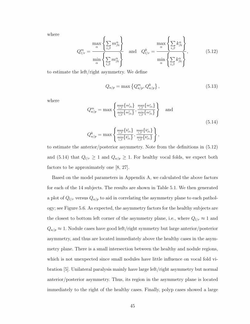
where
Qml/r =
maxα
{∑i,β
mαβi
}
minα
{∑i,β
mαβi
} and Qkl/r =
maxα
{∑i,β
kαβi
}
minα
{∑i,β
kαβi
} , (5.12)
to estimate the left/right asymmetry. We define
Qa/p = max{Qma/p, Q
ka/p
}, (5.13)
where
Qma/p = max
{maxi,β{ml
βi}mini,β{ml
βi},maxi,β{mr
βi}mini,β{mr
βi}
}and
Qka/p = max
{maxi,β{klβi}
mini,β{klβi}
,maxi,β{krβi}
mini,β{krβi}
},
(5.14)
to estimate the anterior/posterior asymmetry. Note from the definitions in (5.12)
and (5.14) that Ql/r ≥ 1 and Qa/p ≥ 1. For healthy vocal folds, we expect both
factors to be approximately one [8, 27].
Based on the model parameters in Appendix A, we calculated the above factors
for each of the 14 subjects. The results are shown in Table 5.1. We then generated
a plot of Ql/r versus Qa/p to aid in correlating the asymmetry plane to each pathol-
ogy; see Figure 5.6. As expected, the asymmetry factors for the healthy subjects are
the closest to bottom left corner of the asymmetry plane, i.e., where Ql/r ≈ 1 and
Qa/p ≈ 1. Nodule cases have good left/right symmetry but large anterior/posterior
asymmetry, and thus are located immediately above the healthy cases in the asym-
metry plane. There is a small intersection between the healthy and nodule regions,
which is not unexpected since small nodules have little influence on vocal fold vi-
bration [5]. Unilateral paralysis mainly have large left/right asymmetry but normal
anterior/posterior asymmetry. Thus, its region in the asymmetry plane is located
immediately to the right of the healthy cases. Finally, polyp cases showed a large
45
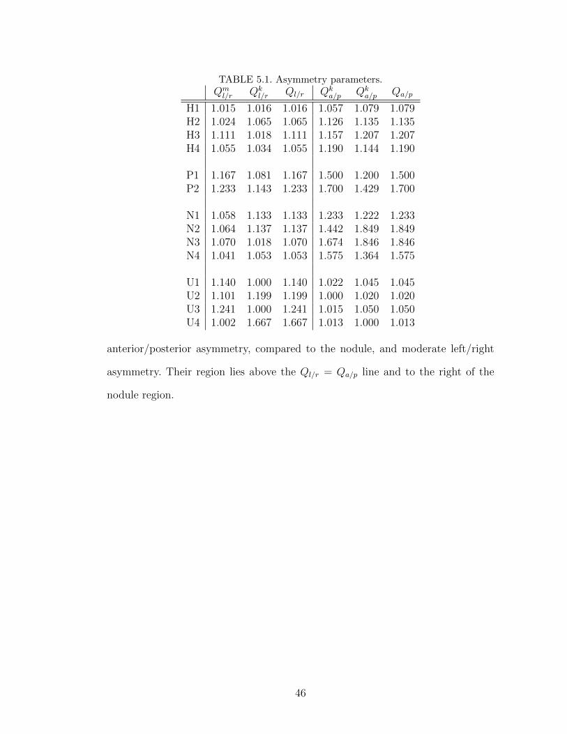
TABLE 5.1. Asymmetry parameters.Qml/r Qk
l/r Ql/r Qka/p Qk
a/p Qa/p
H1 1.015 1.016 1.016 1.057 1.079 1.079H2 1.024 1.065 1.065 1.126 1.135 1.135H3 1.111 1.018 1.111 1.157 1.207 1.207H4 1.055 1.034 1.055 1.190 1.144 1.190
P1 1.167 1.081 1.167 1.500 1.200 1.500P2 1.233 1.143 1.233 1.700 1.429 1.700
N1 1.058 1.133 1.133 1.233 1.222 1.233N2 1.064 1.137 1.137 1.442 1.849 1.849N3 1.070 1.018 1.070 1.674 1.846 1.846N4 1.041 1.053 1.053 1.575 1.364 1.575
U1 1.140 1.000 1.140 1.022 1.045 1.045U2 1.101 1.199 1.199 1.000 1.020 1.020U3 1.241 1.000 1.241 1.015 1.050 1.050U4 1.002 1.667 1.667 1.013 1.000 1.013
anterior/posterior asymmetry, compared to the nodule, and moderate left/right
asymmetry. Their region lies above the Ql/r = Qa/p line and to the right of the
nodule region.
46
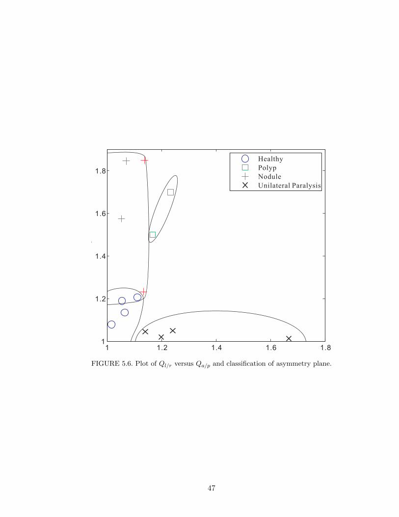
1 1.2 1.4 1.6 1.81
1.2
1.4
1.6
1.8
Healthy
Polyp
Nodule
Unilateral Paralysis
Qa
p/
Ql r/FIGURE 5.6. Plot of Ql/r versus Qa/p and classification of asymmetry plane.
47
Chapter 6Conclusion and Recommendations
Vibration of vocal folds is the main source of voice production. Irregularity in the
sustained vibration of vocal folds is believed to be rooted in physiological changes
in the vocal folds caused by certain disorders. This dissertation introduced a new
biomechanical model for the vibrations of vocal folds that incorporates the most rel-
evant characteristics of the vocal fold dynamics. The proposed lumped-parameter
model utilizes one mass for the vocal fold body tissue and three pairs of upper/lower
masses along the vocal fold length for the cover tissue. A preliminary model val-
idation was presented by evaluating its ability to reproduce the actual vibration
pattern of healthy and pathological (nodule, polyp, and unilateral paralysis) vo-
cal folds obtained experimentally via a high-speed imaging system. The proposed
model was able to match the experimental (frequency- and time-domain) data
relatively well while outperforming an existing model that neglects the mass and
stiffness of the vocal fold body tissue.
Another contribution of this work was the development of a physically-inspired,
semi-empirical tuning procedure for the model parameters. The tuning criteria
were based on the fundamental frequency, amplitude, phase difference, and collision
duration of the vocal fold vibration. Finally, we introduced two factors to quantify
the left/right and anterior/posterior asymmetries of vocal folds. The use of only
two factors facilitates classifying and visualizing how the healthy and pathological
vocal folds relate to these asymmetries. That is, depending on where these factors
are located on the asymmetry plane for a given set of model parameters, one can
tell if the vocal folds are healthy or not and what disorder (nodule, polyp, or
48
unilateral paralysis) is present. This ‘chart’ can potentially further the assessment
and diagnosis of voice disorders in clinical settings.
Our recommendations for future work are as follows:
• The results of this dissertation are based on experimental data from a limited
set of subjects. Therefore, a more detailed study should be conducted using
a larger and statistically-meaningful number of subjects.
• The experimental data was captured by a HSDI system with 2000 fps and
resolution of 120 × 250 pixels. Since the accuracy of the tuning results for
the model parameters is affected by these characteristics, the use of a HSDI
system with higher frame rate and resolution is recommended for future
research.
• The proposed biomechanical model incorporates a commonly-used model
for the collision of the vocal folds. We observed that the model cannot be
adequately tuned to capture the duration of the collision at each segment
of the vocal fold. Therefore, further research efforts should be dedicated to
improving the collision model.
• The fine-tuning algorithm may be improved by introducing and minimizing
other error variables.
49
References
[1] American Speech-Language-Hearing Association, www.asha.org.
[2] T. Baer. Investigation of phonation using excised larynxes. PhD thesis, MIT,Cambridge, MA, 1976.
[3] D.M. Biever and D.M. Bless. Vibratory characteristics of the vocal folds inyoung adult and geriatric women. J. Voice, 3(2):120–131, 1989.
[4] K.F. Chen, J.T. Jiang, and S. Crowsen. Against the long-range spectralleakage of the cosine window family. Computer Physics Communications,180(6):904–911, 2009.
[5] R.H. Colton, J.K. Casper, and R. Leonard. Understanding Voice Problems: APhysiological Perspective for Diagnosis and Treatment. Lippincott Williams& Wilkins, October 2005.
[6] T.H. Crystal. Model of larynx activity during phonation. J. Acoust. Soc.Am., 38(5):934–935, November 1965.
[7] M. Dollinger, U. Hoppe, F. Hettlich, J. Lohscheller, S. Schuberth, and U. Eysh-oldt. Vibration parameter extraction from endoscopic image series of the vocalfolds. Biomedical Engineering, IEEE Transactions on, 49(8):773–781, 2002.
[8] U. Eysholdt, F. Rosanowski, and U. Hoppe. Vocal fold vibration irregularitiescaused by different types of laryngeal asymmetry. European Archives of Oto-Rhino-Laryngology, 260(8):412–417, 2003.
[9] U. Eysholdt, M. Tigges, T. Wittenberg, and U. Proschel. Direct evaluation ofhigh-speed recordings of vocal fold vibrations. Folia Phoniatrica et Logopaed-ica, 48(4):163–170, 1996.
[10] J. L Flanagan. Estimates of intraglottal pressure during phonation. Journalof Speech and Hearing Research, 2(2):168–168, 1959.
[11] J. Flanagan and L. Landgraf. Self-oscillating source for vocal-tract synthesiz-ers. Audio and Electroacoustics, IEEE Transactions on, 16(1):57–64, 1968.
[12] S. Hertegard, H. Larsson, and T. Wittenberg. High-speed imaging: applica-tions and development. Logopedics Phonatrics Vocology, 28(3):133–139, 2003.
[13] M Hirano. Morphological structure of the vocal cord as a vibrator and itsvariations. Folia Phoniatr (Basel), 26(2):89–94, 1974.
[14] M. Hirano and D.M. Bless. Videostroboscopic Examination of the Larynx.Singular Pub. Group, 1993.
50
[15] M. Hirano and Y. Kakita. Cover-body theory of vocal fold vibration. SpeechScience–Recent Advances. College-Hill Press, San Diego, 1985.
[16] K. Ishizaka and J. Flanagan. Synthesis of voiced sounds from a two-massmodel of the vocal cords. The Bell System Technical Journal, 51(6):1233–1268, 1972.
[17] K. Ishizaka and N. Isshiki. Computer simulation of pathological vocal-cordvibration. J. Acoust. Soc. Am., 60(5):1193–1198, November 1976.
[18] J.J. Jiang, Y. Zhang, and J. Stern. Modeling of chaotic vibrations in sym-metric vocal folds. J. Acoust. Soc. Am., 110(4):2120–2128, October 2001.
[19] S.M. Kay. Fundamentals of Statistical Signal Processing, Volume II: DetectionTheory. Upper Saddle River (New Jersey), 1998.
[20] K.A. Kendall, M.M. Browning, and S.M. Skovlund. Introduction to high-speed imaging of the larynx. Current Opinion in Otolaryngology & Head andNeck Surgery, 13(3):135, 2005.
[21] R.D. Kent. The MIT Encyclopedia of Communication Disorders. The MITPress, 2004.
[22] S. Kiritani, H. Imagawa, and H. Hirose. High-speed digital image recording forthe observation of vocal cord vibration. Vocal Physiology: Voice Production,Mechanisms and Functions, pages 261–269, 1988.
[23] K. Kuroki. Subglottic pressure of normal and pathological larynges. Otologia,15:54–74, 1969.
[24] J.C, Lucero and C.A Gajo. Oscillation region of a piecewise-smooth modelof the vocal folds. Communications in Mathematical Sciences, 4(2):453–469,2006.
[25] P. Mergell, H. Herzel, and I.R. Titze. Irregular vocal-fold vibration—high-speed observation and modeling. J. Acoust. Soc. Am., 108(6):2996–3002, De-cember 2000.
[26] X. Ming and D. Kang. Corrections for frequency, amplitude and phase in afast fourier transform of a harmonic signal. Mechanical Systems and SignalProcessing, 10(2):211–221, 1996.
[27] J. Neubauer, P. Mergell, U. Eysholdt, and H. Herzel. Spatio-temporal analysisof irregular vocal fold oscillations: Biphonation due to desynchronization ofspatial modes. J. Acoust. Soc. Am., 110(6):3179–3192, December 2001.
[28] A.V. Oppenheim, A.S. Willsky, and S.H. Nawab. Signals and Systems. Pren-tice Hall, 1997.
51
[29] S. S. Rao. Mechanical Vibrations. Prentice-Hall, Upper Saddle River, NJ,2003.
[30] J. Schoukens, R. Pintelon, and H. Van Hamme. The interpolated fast fouriertransform: A comparative study. Instrumentation and Measurement, IEEETransactions on, 41(2):226–232, 1992.
[31] R. Schwarz, M. Dollinger, T. Wurzbacher, U. Eysholdt, and J. Lohscheller.Spatio-temporal quantification of vocal fold vibrations using high-speedvideoendoscopy and a biomechanical model. J. Acoust. Soc. Am.,123(5):2717–2717, 2008.
[32] I. Steinecke and H. Herzel. Bifurcations in an asymmetric vocal-fold model.J. Acoust. Soc. Am., 97(3):1874–1884, March 1995.
[33] B.H Story and I. R Titze. Voice simulation with a body-cover model of thevocal folds. J. Acoust. Soc. Am., 97(2):1249–1260, 1995.
[34] I.R. Titze. Principles of Voice Production. Prentice-Hall, Englewood Cliffs,NJ, 1994.
[35] I.R. Titze. Myoelastic Aerodynamic Theory of Phonation. Iowa City, IA:NCVS, 2006.
[36] I.R. Titze. The human vocal cords: A mathematical model, part I. Phonetica,28:129-170, 1973.
[37] Z. Wei, M. de Queiroz, J. Chen, B. Gunturk, and M. Kunduk. A new biome-chanical model of vocal fold vibrations: preliminary experimental validation.Proc. ASME Dynamic Syst. and Control Conf., Paper No. DSCC2011-6171,Arlington, VA, 2011.
[38] D. Wong, M.R. Ito, N.B. Cox, and I.R. Titze. Observation of perturbationsin a lumped-element model of the vocal folds with application to some patho-logical cases. J. Acoust Soc. Am., 89(1):383–394, 1991.
[39] T. Wurzbacher, M. Dollinger, R. Schwarz, U. Hoppe, U. Eysholdt, andJ. Lohscheller. Spatiotemporal classification of vocal fold dynamics by a mul-timass model comprising time-dependent parameters. J. Acoust. Soc. Am.,123:2324, 2008.
[40] T. Wurzbacher, R. Schwarz, M. Dollinger, U. Hoppe, U. Eysholdt, and J.Lohscheller. Model-based classification of nonstationary vocal fold vibrations.J. Acoust. Soc. Am., 120(2):1012–1027, 2006.
[41] Y. Yan, K. Ahmad, M. Kunduk, and D. Bless. Analysis of vocal-fold vi-brations from high-speed laryngeal images using a Hilbert transform-basedmethodology. J. Voice, 19(2):161–175, June 2005.
52
Appendix AParameter Tuning Results
The following tables compile the parameters that resulted from applying the full
tuning process of Chapter 4 to the 14 sets of experimental data. The parameter
values without units in the tables represent multiplicative factors applied to the
corresponding initial values. For example, mlβ1 = 0.936 in the first column of
Table A.1 means 93.6% of the corresponding parameter value given in (3.10).
53
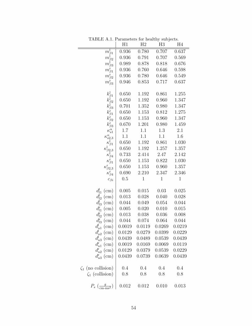
TABLE A.1. Parameters for healthy subjects.H1 H2 H3 H4
mlβ1 0.936 0.780 0.707 0.637
mlβ2 0.936 0.791 0.707 0.569
mlβ3 0.989 0.878 0.818 0.676
mrβ1 0.936 0.760 0.646 0.598
mrβ2 0.936 0.780 0.646 0.549
mrβ3 0.946 0.853 0.717 0.637
klβ1 0.650 1.192 0.861 1.255klβ2 0.650 1.192 0.960 1.347klβ3 0.701 1.352 0.980 1.347krβ1 0.650 1.153 0.812 1.275krβ2 0.650 1.153 0.960 1.347krβ3 0.670 1.201 0.980 1.459καs1 1.7 1.1 1.3 2.1καs2,3 1.1 1.1 1.1 1.6κlβ1 0.650 1.192 0.861 1.030κlβ2,3 0.650 1.192 1.257 1.357κlβ4 0.733 2.414 2.47 2.142κrβ1 0.650 1.153 0.822 1.030κrβ2,3 0.650 1.153 0.960 1.357κrβ4 0.690 2.210 2.347 2.346cβi 0.5 1 1 1
dll1 (cm) 0.005 0.015 0.03 0.025dll2 (cm) 0.013 0.028 0.040 0.028dll3 (cm) 0.044 0.049 0.054 0.044drl1 (cm) 0.005 0.020 0.010 0.015drl2 (cm) 0.013 0.038 0.036 0.008drl3 (cm) 0.044 0.074 0.064 0.044dlu1 (cm) 0.0019 0.0119 0.0269 0.0219dlu2 (cm) 0.0129 0.0279 0.0399 0.0229dlu3 (cm) 0.0439 0.0489 0.0539 0.0439dru1 (cm) 0.0019 0.0169 0.0069 0.0119dru2 (cm) 0.0129 0.0379 0.0539 0.0229dru3 (cm) 0.0439 0.0739 0.0639 0.0439
ζ1 (no collision) 0.4 0.4 0.4 0.4ζ1 (collision) 0.8 0.8 0.8 0.8
Ps ( gcm-ms2
) 0.012 0.012 0.010 0.013
54
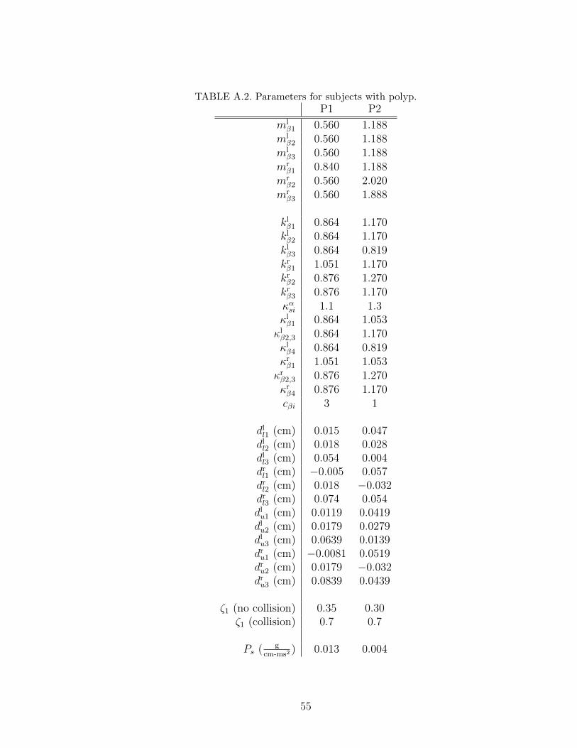
TABLE A.2. Parameters for subjects with polyp.P1 P2
mlβ1 0.560 1.188
mlβ2 0.560 1.188
mlβ3 0.560 1.188
mrβ1 0.840 1.188
mrβ2 0.560 2.020
mrβ3 0.560 1.888
klβ1 0.864 1.170klβ2 0.864 1.170klβ3 0.864 0.819krβ1 1.051 1.170krβ2 0.876 1.270krβ3 0.876 1.170καsi 1.1 1.3κlβ1 0.864 1.053κlβ2,3 0.864 1.170κlβ4 0.864 0.819κrβ1 1.051 1.053κrβ2,3 0.876 1.270κrβ4 0.876 1.170cβi 3 1
dll1 (cm) 0.015 0.047dll2 (cm) 0.018 0.028dll3 (cm) 0.054 0.004drl1 (cm) −0.005 0.057drl2 (cm) 0.018 −0.032drl3 (cm) 0.074 0.054dlu1 (cm) 0.0119 0.0419dlu2 (cm) 0.0179 0.0279dlu3 (cm) 0.0639 0.0139dru1 (cm) −0.0081 0.0519dru2 (cm) 0.0179 −0.032dru3 (cm) 0.0839 0.0439
ζ1 (no collision) 0.35 0.30ζ1 (collision) 0.7 0.7
Ps ( gcm-ms2
) 0.013 0.004
55
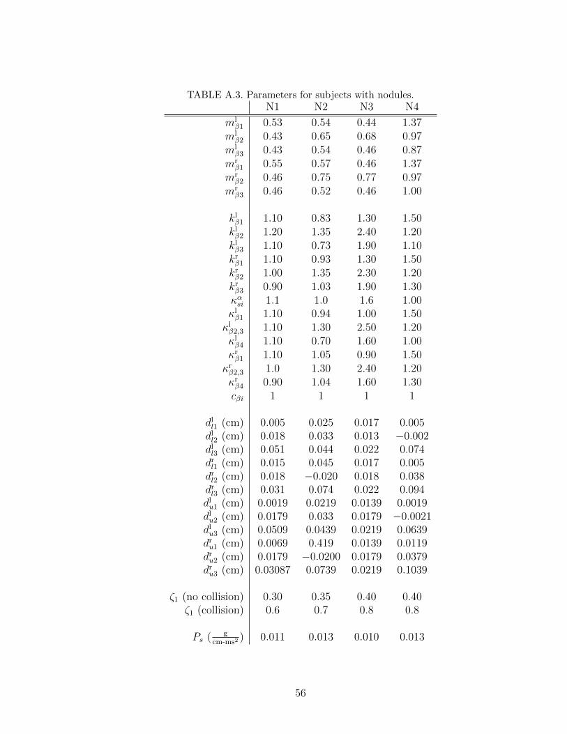
TABLE A.3. Parameters for subjects with nodules.N1 N2 N3 N4
mlβ1 0.53 0.54 0.44 1.37
mlβ2 0.43 0.65 0.68 0.97
mlβ3 0.43 0.54 0.46 0.87
mrβ1 0.55 0.57 0.46 1.37
mrβ2 0.46 0.75 0.77 0.97
mrβ3 0.46 0.52 0.46 1.00
klβ1 1.10 0.83 1.30 1.50klβ2 1.20 1.35 2.40 1.20klβ3 1.10 0.73 1.90 1.10krβ1 1.10 0.93 1.30 1.50krβ2 1.00 1.35 2.30 1.20krβ3 0.90 1.03 1.90 1.30καsi 1.1 1.0 1.6 1.00κlβ1 1.10 0.94 1.00 1.50κlβ2,3 1.10 1.30 2.50 1.20κlβ4 1.10 0.70 1.60 1.00κrβ1 1.10 1.05 0.90 1.50κrβ2,3 1.0 1.30 2.40 1.20κrβ4 0.90 1.04 1.60 1.30cβi 1 1 1 1
dll1 (cm) 0.005 0.025 0.017 0.005dll2 (cm) 0.018 0.033 0.013 −0.002dll3 (cm) 0.051 0.044 0.022 0.074drl1 (cm) 0.015 0.045 0.017 0.005drl2 (cm) 0.018 −0.020 0.018 0.038drl3 (cm) 0.031 0.074 0.022 0.094dlu1 (cm) 0.0019 0.0219 0.0139 0.0019dlu2 (cm) 0.0179 0.033 0.0179 −0.0021dlu3 (cm) 0.0509 0.0439 0.0219 0.0639dru1 (cm) 0.0069 0.419 0.0139 0.0119dru2 (cm) 0.0179 −0.0200 0.0179 0.0379dru3 (cm) 0.03087 0.0739 0.0219 0.1039
ζ1 (no collision) 0.30 0.35 0.40 0.40ζ1 (collision) 0.6 0.7 0.8 0.8
Ps ( gcm-ms2
) 0.011 0.013 0.010 0.013
56
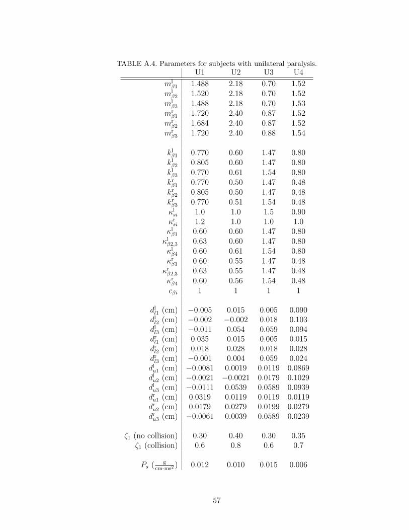
TABLE A.4. Parameters for subjects with unilateral paralysis.U1 U2 U3 U4
mlβ1 1.488 2.18 0.70 1.52
mlβ2 1.520 2.18 0.70 1.52
mlβ3 1.488 2.18 0.70 1.53
mrβ1 1.720 2.40 0.87 1.52
mrβ2 1.684 2.40 0.87 1.52
mrβ3 1.720 2.40 0.88 1.54
klβ1 0.770 0.60 1.47 0.80klβ2 0.805 0.60 1.47 0.80klβ3 0.770 0.61 1.54 0.80krβ1 0.770 0.50 1.47 0.48krβ2 0.805 0.50 1.47 0.48krβ3 0.770 0.51 1.54 0.48κlsi 1.0 1.0 1.5 0.90κrsi 1.2 1.0 1.0 1.0κlβ1 0.60 0.60 1.47 0.80κlβ2,3 0.63 0.60 1.47 0.80κlβ4 0.60 0.61 1.54 0.80κrβ1 0.60 0.55 1.47 0.48κrβ2,3 0.63 0.55 1.47 0.48κrβ4 0.60 0.56 1.54 0.48cβi 1 1 1 1
dll1 (cm) −0.005 0.015 0.005 0.090dll2 (cm) −0.002 −0.002 0.018 0.103dll3 (cm) −0.011 0.054 0.059 0.094drl1 (cm) 0.035 0.015 0.005 0.015drl2 (cm) 0.018 0.028 0.018 0.028drl3 (cm) −0.001 0.004 0.059 0.024dlu1 (cm) −0.0081 0.0019 0.0119 0.0869dlu2 (cm) −0.0021 −0.0021 0.0179 0.1029dlu3 (cm) −0.0111 0.0539 0.0589 0.0939dru1 (cm) 0.0319 0.0119 0.0119 0.0119dru2 (cm) 0.0179 0.0279 0.0199 0.0279dru3 (cm) −0.0061 0.0039 0.0589 0.0239
ζ1 (no collision) 0.30 0.40 0.30 0.35ζ1 (collision) 0.6 0.8 0.6 0.7
Ps ( gcm-ms2
) 0.012 0.010 0.015 0.006
57
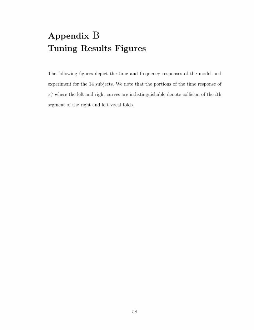
Appendix BTuning Results Figures
The following figures depict the time and frequency responses of the model and
experiment for the 14 subjects. We note that the portions of the time response of
xαi where the left and right curves are indistinguishable denote collision of the ith
segment of the right and left vocal folds.
58
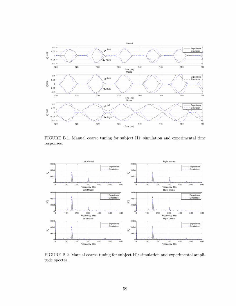
120 125 130 135 140 145 150 155
−0.1
−0.05
0
0.05
0.1
Time (ms)
xα 1 (
cm
)
Ventral
Experiment
Simulation
120 125 130 135 140 145 150 155
−0.1
−0.05
0
0.05
0.1
Time (ms)
xα 2 (
cm
)
Medial
Experiment
Simulation
120 125 130 135 140 145 150 155
−0.1
−0.05
0
0.05
0.1
Time (ms)
xα 3 (
cm
)
Dorsal
Experiment
Simulation
Left
Left
Right
Right
Left
Right
FIGURE B.1. Manual coarse tuning for subject H1: simulation and experimental timeresponses.
0 100 200 300 400 500 6000
0.02
0.04
0.06Left Ventral
Frequency (Hz)
|Xl 1|
Experiment
Simulation
0 100 200 300 400 500 6000
0.02
0.04
0.06Right Ventral
Frequency (Hz)
|Xr 1|
Experiment
Simulation
0 100 200 300 400 500 6000
0.02
0.04
0.06Left Medial
Frequency (Hz)
|Xl 2|
Experiment
Simulation
0 100 200 300 400 500 6000
0.02
0.04
0.06Right Medial
Frequency (Hz)
|Xr 2|
Experiment
Simulation
0 100 200 300 400 500 6000
0.02
0.04
0.06Left Dorsal
Frequency (Hz)
|Xl 3|
Experiment
Simulation
0 100 200 300 400 500 6000
0.02
0.04
0.06Right Dorsal
Frequency (Hz)
|Xr 3|
Experiment
Simulation
FIGURE B.2. Manual coarse tuning for subject H1: simulation and experimental ampli-tude spectra.
59
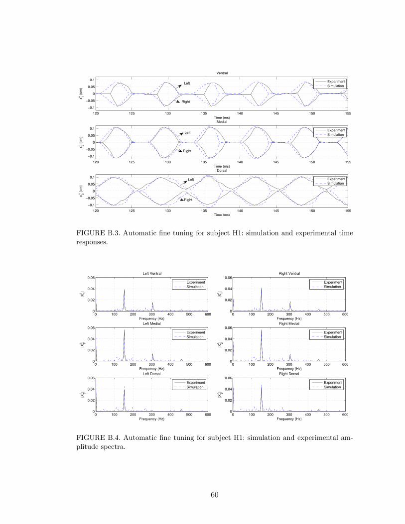
120 125 130 135 140 145 150 155
−0.1
−0.05
0
0.05
0.1
Time (ms)
xα 1 (
cm
)
Ventral
Experiment
Simulation
120 125 130 135 140 145 150 155
−0.1
−0.05
0
0.05
0.1
Time (ms)
xα 2 (
cm
)
Medial
Experiment
Simulation
120 125 130 135 140 145 150 155
−0.1
−0.05
0
0.05
0.1
Time (ms)
xα 3 (
cm
)
Dorsal
Experiment
Simulation
Right
Left
Right
Left
Left
Right
FIGURE B.3. Automatic fine tuning for subject H1: simulation and experimental timeresponses.
0 100 200 300 400 500 6000
0.02
0.04
0.06Left Ventral
Frequency (Hz)
|Xl 1|
Experiment
Simulation
0 100 200 300 400 500 6000
0.02
0.04
0.06Right Ventral
Frequency (Hz)
|Xr 1|
Experiment
Simulation
0 100 200 300 400 500 6000
0.02
0.04
0.06Left Medial
Frequency (Hz)
|Xl 2|
Experiment
Simulation
0 100 200 300 400 500 6000
0.02
0.04
0.06Right Medial
Frequency (Hz)
|Xr 2|
Experiment
Simulation
0 100 200 300 400 500 6000
0.02
0.04
0.06Left Dorsal
Frequency (Hz)
|Xl 3|
Experiment
Simulation
0 100 200 300 400 500 6000
0.02
0.04
0.06Right Dorsal
Frequency (Hz)
|Xr 3|
Experiment
Simulation
FIGURE B.4. Automatic fine tuning for subject H1: simulation and experimental am-plitude spectra.
60
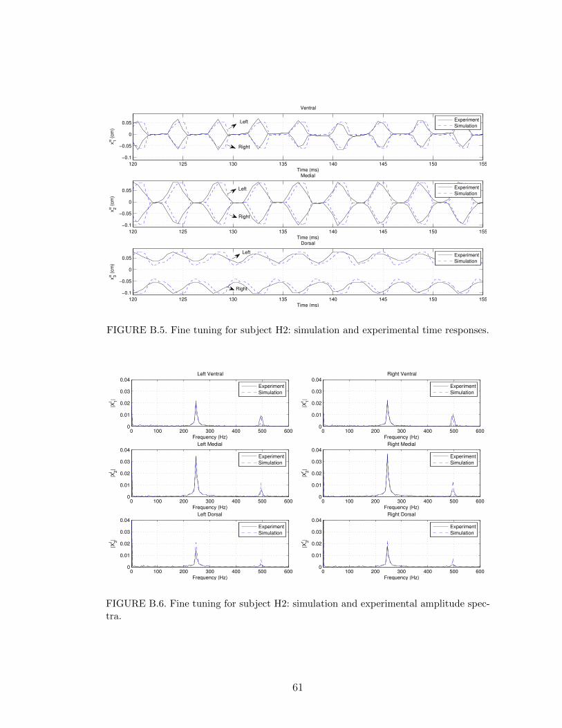
120 125 130 135 140 145 150 155
−0.1
−0.05
0
0.05
Time (ms)
xα 1 (
cm
)Ventral
Experiment
Simulation
120 125 130 135 140 145 150 155
−0.1
−0.05
0
0.05
Time (ms)
xα 2 (
cm
)
Medial
Experiment
Simulation
120 125 130 135 140 145 150 155
−0.1
−0.05
0
0.05
Time (ms)
xα 3 (
cm
)
Dorsal
Experiment
Simulation
Left
Right
Left
Right
Left
Right
FIGURE B.5. Fine tuning for subject H2: simulation and experimental time responses.
0 100 200 300 400 500 6000
0.01
0.02
0.03
0.04Left Ventral
Frequency (Hz)
|Xl 1|
Experiment
Simulation
0 100 200 300 400 500 6000
0.01
0.02
0.03
0.04Right Ventral
Frequency (Hz)
|Xr 1|
Experiment
Simulation
0 100 200 300 400 500 6000
0.01
0.02
0.03
0.04Left Medial
Frequency (Hz)
|Xl 2|
Experiment
Simulation
0 100 200 300 400 500 6000
0.01
0.02
0.03
0.04Right Medial
Frequency (Hz)
|Xr 2|
Experiment
Simulation
0 100 200 300 400 500 6000
0.01
0.02
0.03
0.04Left Dorsal
Frequency (Hz)
|Xl 3|
Experiment
Simulation
0 100 200 300 400 500 6000
0.01
0.02
0.03
0.04Right Dorsal
Frequency (Hz)
|Xr 3|
Experiment
Simulation
FIGURE B.6. Fine tuning for subject H2: simulation and experimental amplitude spec-tra.
61
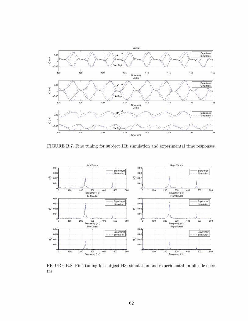
120 125 130 135 140 145 150 155
−0.05
0
0.05
Time (ms)
xα 1 (
cm
)Ventral
Experiment
Simulation
120 125 130 135 140 145 150 155
−0.05
0
0.05
Time (ms)
xα 2 (
cm
)
Medial
Experiment
Simulation
120 125 130 135 140 145 150 155
−0.05
0
0.05
Time (ms)
xα 3 (
cm
)
Dorsal
Experiment
Simulation
Left
Right
Left
Right
Left
Right
FIGURE B.7. Fine tuning for subject H3: simulation and experimental time responses.
0 100 200 300 400 500 6000
0.01
0.02
0.03
0.04Left Ventral
Frequency (Hz)
|Xl 1|
Experiment
Simulation
0 100 200 300 400 500 6000
0.01
0.02
0.03
0.04Right Ventral
Frequency (Hz)
|Xr 1|
Experiment
Simulation
0 100 200 300 400 500 6000
0.01
0.02
0.03
0.04Left Medial
Frequency (Hz)
|Xl 2|
Experiment
Simulation
0 100 200 300 400 500 6000
0.01
0.02
0.03
0.04Right Medial
Frequency (Hz)
|Xr 2|
Experiment
Simulation
0 100 200 300 400 500 6000
0.01
0.02
0.03
0.04Left Dorsal
Frequency (Hz)
|Xl 3|
Experiment
Simulation
0 100 200 300 400 500 6000
0.01
0.02
0.03
0.04Right Dorsal
Frequency (Hz)
|Xr 3|
Experiment
Simulation
FIGURE B.8. Fine tuning for subject H3: simulation and experimental amplitude spec-tra.
62
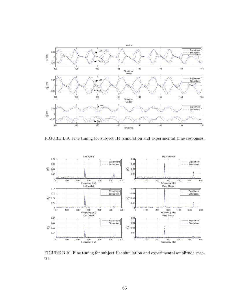
120 125 130 135 140 145 150 155
−0.05
0
0.05
Time (ms)
xα 1 (
cm
)Ventral
Experiment
Simulation
120 125 130 135 140 145 150 155
−0.05
0
0.05
Time (ms)
xα 2 (
cm
)
Medial
Experiment
Simulation
120 125 130 135 140 145 150 155
−0.05
0
0.05
Time (ms)
xα 3 (
cm
)
Dorsal
Experiment
Simulation
Left
Right
Left
Right
Left
Right
FIGURE B.9. Fine tuning for subject H4: simulation and experimental time responses.
0 100 200 300 400 500 6000
0.01
0.02
0.03
0.04Left Ventral
Frequency (Hz)
|Xl 1|
Experiment
Simulation
0 100 200 300 400 500 6000
0.01
0.02
0.03
0.04Right Ventral
Frequency (Hz)
|Xr 1|
Experiment
Simulation
0 100 200 300 400 500 6000
0.01
0.02
0.03
0.04Left Medial
Frequency (Hz)
|Xl 2|
Experiment
Simulation
0 100 200 300 400 500 6000
0.01
0.02
0.03
0.04Right Medial
Frequency (Hz)
|Xr 2|
Experiment
Simulation
0 100 200 300 400 500 6000
0.01
0.02
0.03
0.04Left Dorsal
Frequency (Hz)
|Xl 3|
Experiment
Simulation
0 100 200 300 400 500 6000
0.01
0.02
0.03
0.04Right Dorsal
Frequency (Hz)
|Xr 3|
Experiment
Simulation
FIGURE B.10. Fine tuning for subject H4: simulation and experimental amplitude spec-tra.
63
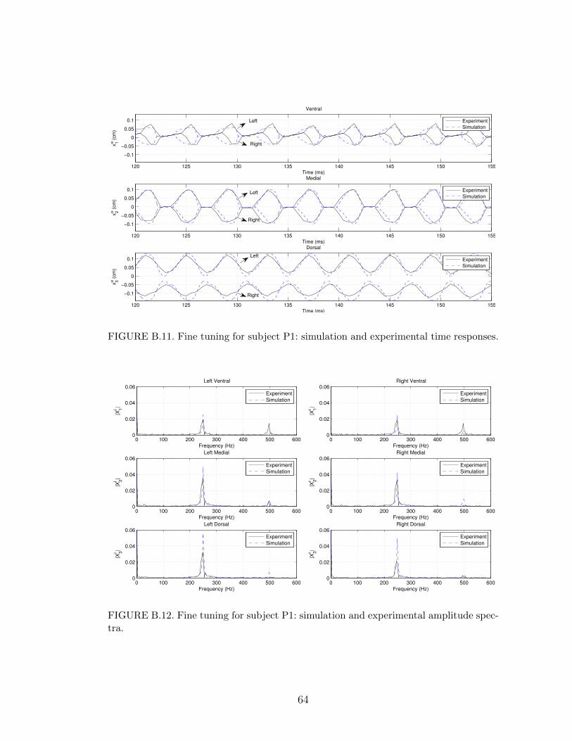
120 125 130 135 140 145 150 155
−0.1
−0.05
0
0.05
0.1
Time (ms)
xα 1 (
cm
)Ventral
Experiment
Simulation
120 125 130 135 140 145 150 155
−0.1
−0.05
0
0.05
0.1
Time (ms)
xα 2 (
cm
)
Medial
Experiment
Simulation
120 125 130 135 140 145 150 155
−0.1
−0.05
0
0.05
0.1
Time (ms)
xα 3 (
cm
)
Dorsal
Experiment
Simulation
Left
Right
Left
Right
Right
Left
FIGURE B.11. Fine tuning for subject P1: simulation and experimental time responses.
0 100 200 300 400 500 6000
0.02
0.04
0.06Left Ventral
Frequency (Hz)
|Xl 1|
Experiment
Simulation
0 100 200 300 400 500 6000
0.02
0.04
0.06Right Ventral
Frequency (Hz)
|Xr 1|
Experiment
Simulation
0 100 200 300 400 500 6000
0.02
0.04
0.06Left Medial
Frequency (Hz)
|Xl 2|
Experiment
Simulation
0 100 200 300 400 500 6000
0.02
0.04
0.06Right Medial
Frequency (Hz)
|Xr 2|
Experiment
Simulation
0 100 200 300 400 500 6000
0.02
0.04
0.06Left Dorsal
Frequency (Hz)
|Xl 3|
Experiment
Simulation
0 100 200 300 400 500 6000
0.02
0.04
0.06Right Dorsal
Frequency (Hz)
|Xr 3|
Experiment
Simulation
FIGURE B.12. Fine tuning for subject P1: simulation and experimental amplitude spec-tra.
64
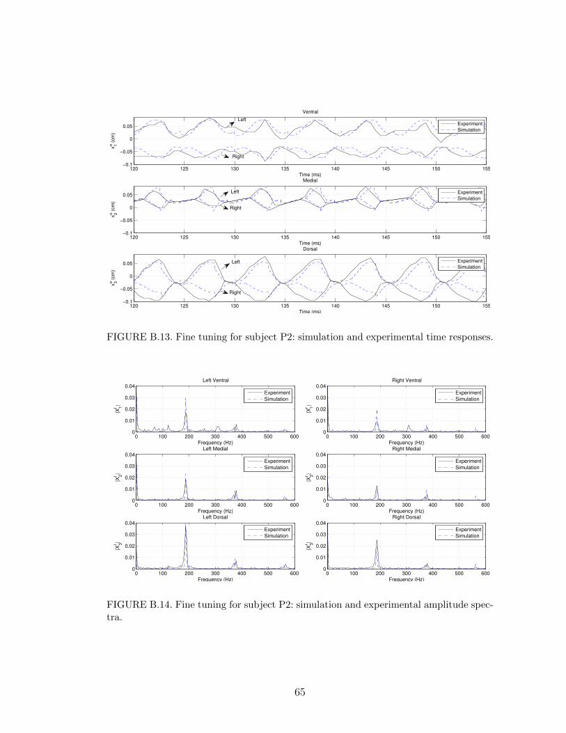
120 125 130 135 140 145 150 155−0.1
−0.05
0
0.05
Time (ms)
xα 1 (
cm
)Ventral
Experiment
Simulation
120 125 130 135 140 145 150 155−0.1
−0.05
0
0.05
Time (ms)
xα 2 (
cm
)
Medial
Experiment
Simulation
120 125 130 135 140 145 150 155−0.1
−0.05
0
0.05
Time (ms)
xα 3 (
cm
)
Dorsal
Experiment
Simulation
Left
Right
Left
Right
Left
Right
FIGURE B.13. Fine tuning for subject P2: simulation and experimental time responses.
0 100 200 300 400 500 6000
0.01
0.02
0.03
0.04Left Ventral
Frequency (Hz)
|Xl 1|
Experiment
Simulation
0 100 200 300 400 500 6000
0.01
0.02
0.03
0.04Right Ventral
Frequency (Hz)
|Xr 1|
Experiment
Simulation
0 100 200 300 400 500 6000
0.01
0.02
0.03
0.04Left Medial
Frequency (Hz)
|Xl 2|
Experiment
Simulation
0 100 200 300 400 500 6000
0.01
0.02
0.03
0.04Right Medial
Frequency (Hz)
|Xr 2|
Experiment
Simulation
0 100 200 300 400 500 6000
0.01
0.02
0.03
0.04Left Dorsal
Frequency (Hz)
|Xl 3|
Experiment
Simulation
0 100 200 300 400 500 6000
0.01
0.02
0.03
0.04Right Dorsal
Frequency (Hz)
|Xr 3|
Experiment
Simulation
FIGURE B.14. Fine tuning for subject P2: simulation and experimental amplitude spec-tra.
65
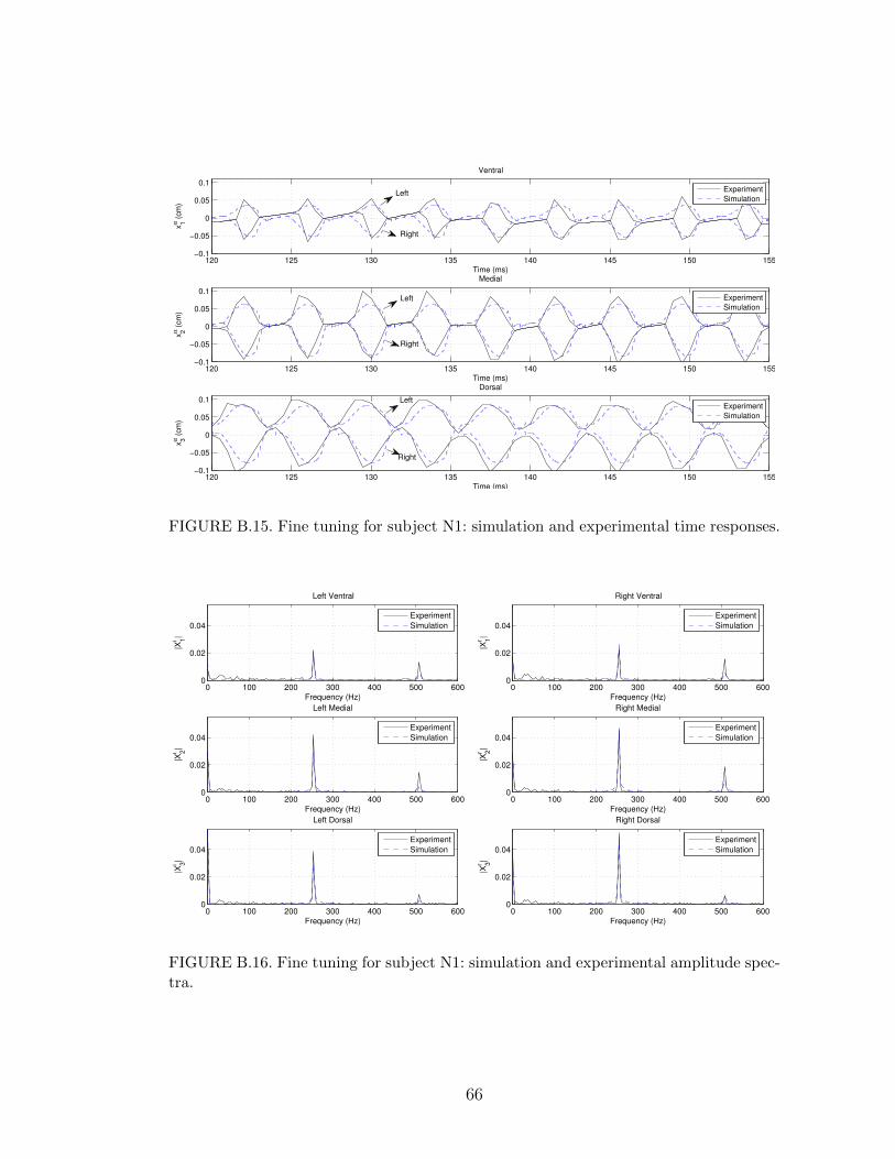
120 125 130 135 140 145 150 155−0.1
−0.05
0
0.05
0.1
Time (ms)
xα 1 (
cm
)Ventral
Experiment
Simulation
120 125 130 135 140 145 150 155−0.1
−0.05
0
0.05
0.1
Time (ms)
xα 2 (
cm
)
Medial
Experiment
Simulation
120 125 130 135 140 145 150 155−0.1
−0.05
0
0.05
0.1
Time (ms)
xα 3 (
cm
)
Dorsal
Experiment
Simulation
Left
Right
Left
Right
Left
Right
FIGURE B.15. Fine tuning for subject N1: simulation and experimental time responses.
0 100 200 300 400 500 6000
0.02
0.04
Left Ventral
Frequency (Hz)
|Xl 1|
Experiment
Simulation
0 100 200 300 400 500 6000
0.02
0.04
Right Ventral
Frequency (Hz)
|Xr 1|
Experiment
Simulation
0 100 200 300 400 500 6000
0.02
0.04
Left Medial
Frequency (Hz)
|Xl 2|
Experiment
Simulation
0 100 200 300 400 500 6000
0.02
0.04
Right Medial
Frequency (Hz)
|Xr 2|
Experiment
Simulation
0 100 200 300 400 500 6000
0.02
0.04
Left Dorsal
Frequency (Hz)
|Xl 3|
Experiment
Simulation
0 100 200 300 400 500 6000
0.02
0.04
Right Dorsal
Frequency (Hz)
|Xr 3|
Experiment
Simulation
FIGURE B.16. Fine tuning for subject N1: simulation and experimental amplitude spec-tra.
66
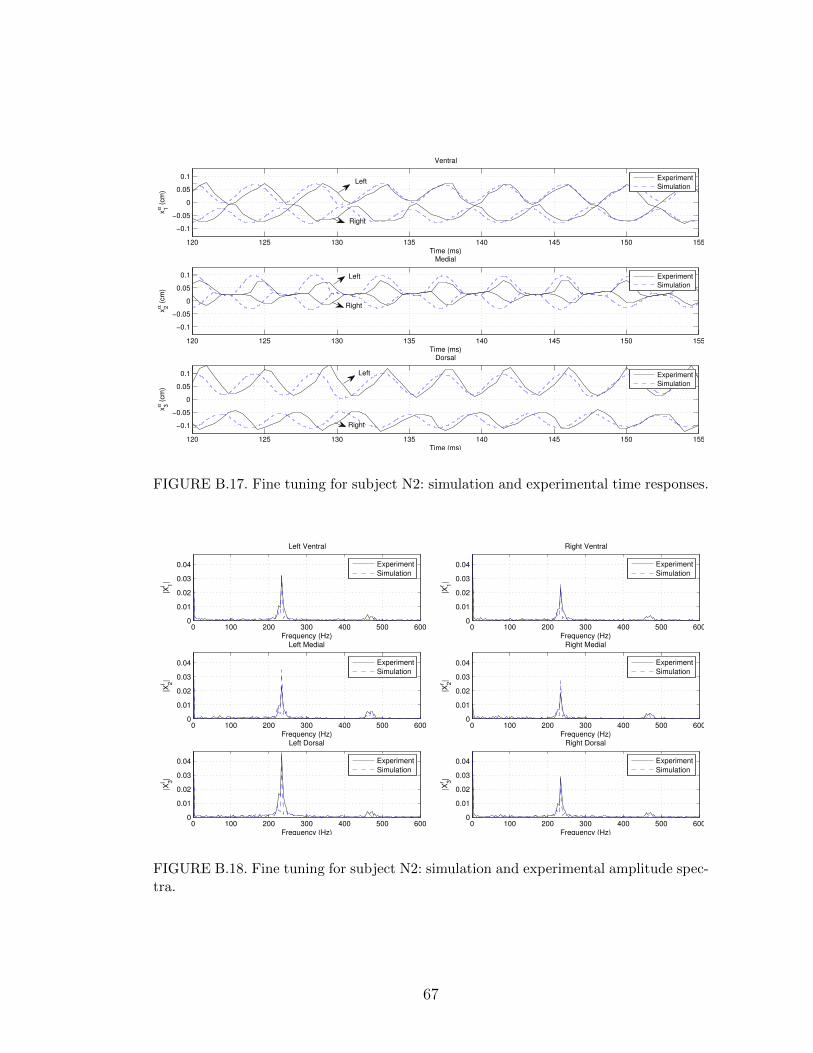
120 125 130 135 140 145 150 155
−0.1
−0.05
0
0.05
0.1
Time (ms)
xα 1 (
cm
)Ventral
Experiment
Simulation
120 125 130 135 140 145 150 155
−0.1
−0.05
0
0.05
0.1
Time (ms)
xα 2 (
cm
)
Medial
Experiment
Simulation
120 125 130 135 140 145 150 155
−0.1
−0.05
0
0.05
0.1
Time (ms)
xα 3 (
cm
)
Dorsal
Experiment
Simulation
Left
Right
Left
Right
Left
Right
FIGURE B.17. Fine tuning for subject N2: simulation and experimental time responses.
0 100 200 300 400 500 6000
0.01
0.02
0.03
0.04
Left Ventral
Frequency (Hz)
|Xl 1|
Experiment
Simulation
0 100 200 300 400 500 6000
0.01
0.02
0.03
0.04
Right Ventral
Frequency (Hz)
|Xr 1|
Experiment
Simulation
0 100 200 300 400 500 6000
0.01
0.02
0.03
0.04
Left Medial
Frequency (Hz)
|Xl 2|
Experiment
Simulation
0 100 200 300 400 500 6000
0.01
0.02
0.03
0.04
Right Medial
Frequency (Hz)
|Xr 2|
Experiment
Simulation
0 100 200 300 400 500 6000
0.01
0.02
0.03
0.04
Left Dorsal
Frequency (Hz)
|Xl 3|
Experiment
Simulation
0 100 200 300 400 500 6000
0.01
0.02
0.03
0.04
Right Dorsal
Frequency (Hz)
|Xr 3|
Experiment
Simulation
FIGURE B.18. Fine tuning for subject N2: simulation and experimental amplitude spec-tra.
67
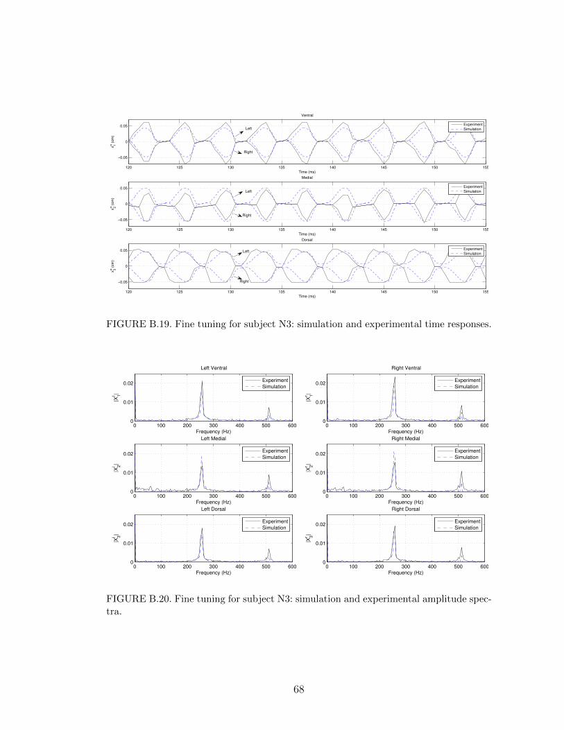
120 125 130 135 140 145 150 155
−0.05
0
0.05
Time (ms)
xα 1 (
cm
)Ventral
Experiment
Simulation
120 125 130 135 140 145 150 155
−0.05
0
0.05
Time (ms)
xα 2 (
cm
)
Medial
Experiment
Simulation
120 125 130 135 140 145 150 155
−0.05
0
0.05
Time (ms)
xα 3 (
cm
)
Dorsal
Experiment
Simulation
Left
Right
Left
Right
Left
Right
FIGURE B.19. Fine tuning for subject N3: simulation and experimental time responses.
0 100 200 300 400 500 6000
0.01
0.02
Left Ventral
Frequency (Hz)
|Xl 1|
Experiment
Simulation
0 100 200 300 400 500 6000
0.01
0.02
Right Ventral
Frequency (Hz)
|Xr 1|
Experiment
Simulation
0 100 200 300 400 500 6000
0.01
0.02
Left Medial
Frequency (Hz)
|Xl 2|
Experiment
Simulation
0 100 200 300 400 500 6000
0.01
0.02
Right Medial
Frequency (Hz)
|Xr 2|
Experiment
Simulation
0 100 200 300 400 500 6000
0.01
0.02
Left Dorsal
Frequency (Hz)
|Xl 3|
Experiment
Simulation
0 100 200 300 400 500 6000
0.01
0.02
Right Dorsal
Frequency (Hz)
|Xr 3|
Experiment
Simulation
FIGURE B.20. Fine tuning for subject N3: simulation and experimental amplitude spec-tra.
68
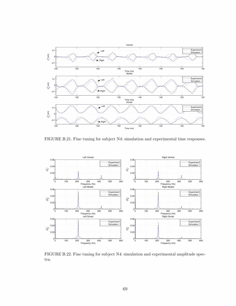
120 125 130 135 140 145 150 155
−0.1
0
0.1
Time (ms)
xα 1 (
cm
)
Ventral
Experiment
Simulation
120 125 130 135 140 145 150 155
−0.1
0
0.1
Time (ms)
xα 2 (
cm
)
Medial
Experiment
Simulation
120 125 130 135 140 145 150 155
−0.1
0
0.1
Time (ms)
xα 3 (
cm
)
Dorsal
Experiment
Simulation
Right
Left
Left
Right
Left
Right
FIGURE B.21. Fine tuning for subject N4: simulation and experimental time responses.
0 100 200 300 400 500 6000
0.02
0.04
0.06Left Ventral
Frequency (Hz)
|Xl 1|
Experiment
Simulation
0 100 200 300 400 500 6000
0.02
0.04
0.06Right Ventral
Frequency (Hz)
|Xr 1|
Experiment
Simulation
0 100 200 300 400 500 6000
0.02
0.04
0.06Left Medial
Frequency (Hz)
|Xl 2|
Experiment
Simulation
0 100 200 300 400 500 6000
0.02
0.04
0.06Right Medial
Frequency (Hz)
|Xr 2|
Experiment
Simulation
0 100 200 300 400 500 6000
0.02
0.04
0.06Left Dorsal
Frequency (Hz)
|Xl 3|
Experiment
Simulation
0 100 200 300 400 500 6000
0.02
0.04
0.06Right Dorsal
Frequency (Hz)
|Xr 3|
Experiment
Simulation
FIGURE B.22. Fine tuning for subject N4: simulation and experimental amplitude spec-tra.
69
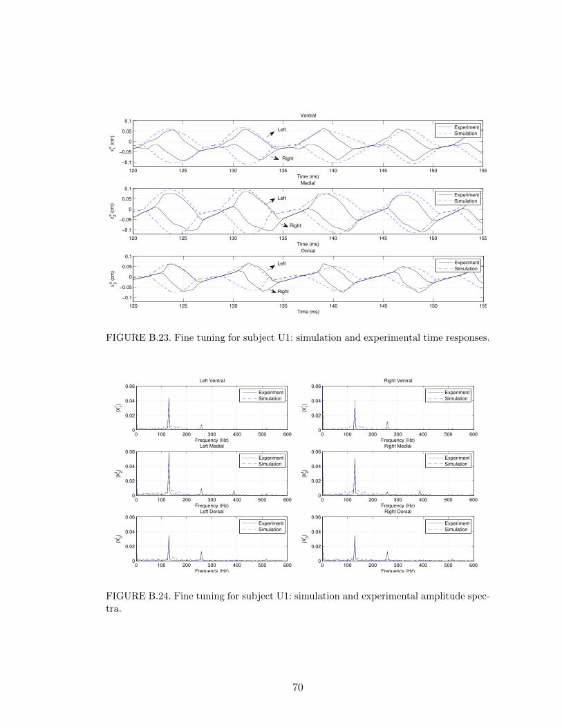
120 125 130 135 140 145 150 155
−0.1
−0.05
0
0.05
0.1
Time (ms)
xα 1 (
cm
)Ventral
Experiment
Simulation
120 125 130 135 140 145 150 155
−0.1
−0.05
0
0.05
0.1
Time (ms)
xα 2 (
cm
)
Medial
Experiment
Simulation
120 125 130 135 140 145 150 155
−0.1
−0.05
0
0.05
0.1
Time (ms)
xα 3 (
cm
)
Dorsal
Experiment
Simulation
Left
Left
Left
Right
Right
Right
FIGURE B.23. Fine tuning for subject U1: simulation and experimental time responses.
0 100 200 300 400 500 6000
0.02
0.04
0.06Left Ventral
Frequency (Hz)
|Xl 1|
Experiment
Simulation
0 100 200 300 400 500 6000
0.02
0.04
0.06Right Ventral
Frequency (Hz)
|Xr 1|
Experiment
Simulation
0 100 200 300 400 500 6000
0.02
0.04
0.06Left Medial
Frequency (Hz)
|Xl 2|
Experiment
Simulation
0 100 200 300 400 500 6000
0.02
0.04
0.06Right Medial
Frequency (Hz)
|Xr 2|
Experiment
Simulation
0 100 200 300 400 500 6000
0.02
0.04
0.06Left Dorsal
Frequency (Hz)
|Xl 3|
Experiment
Simulation
0 100 200 300 400 500 6000
0.02
0.04
0.06Right Dorsal
Frequency (Hz)
|Xr 3|
Experiment
Simulation
FIGURE B.24. Fine tuning for subject U1: simulation and experimental amplitude spec-tra.
70
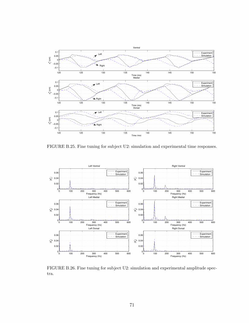
120 125 130 135 140 145 150 155
−0.1
−0.05
0
0.05
0.1
Time (ms)
xα 1 (
cm
)Ventral
Experiment
Simulation
120 125 130 135 140 145 150 155
−0.1
−0.05
0
0.05
0.1
Time (ms)
xα 2 (
cm
)
Medial
Experiment
Simulation
120 125 130 135 140 145 150 155
−0.1
−0.05
0
0.05
0.1
Time (ms)
xα 3 (
cm
)
Dorsal
Experiment
Simulation
Left
Right
Left
Right
Right
Left
FIGURE B.25. Fine tuning for subject U2: simulation and experimental time responses.
0 100 200 300 400 500 6000
0.02
0.04
0.06
Left Ventral
Frequency (Hz)
|Xl 1|
Experiment
Simulation
0 100 200 300 400 500 6000
0.02
0.04
0.06
Right Ventral
Frequency (Hz)
|Xr 1|
Experiment
Simulation
0 100 200 300 400 500 6000
0.02
0.04
0.06
Left Medial
Frequency (Hz)
|Xl 2|
Experiment
Simulation
0 100 200 300 400 500 6000
0.02
0.04
0.06
Right Medial
Frequency (Hz)
|Xr 2|
Experiment
Simulation
0 100 200 300 400 500 6000
0.02
0.04
0.06
Left Dorsal
Frequency (Hz)
|Xl 3|
Experiment
Simulation
0 100 200 300 400 500 6000
0.02
0.04
0.06
Right Dorsal
Frequency (Hz)
|Xr 3|
Experiment
Simulation
FIGURE B.26. Fine tuning for subject U2: simulation and experimental amplitude spec-tra.
71
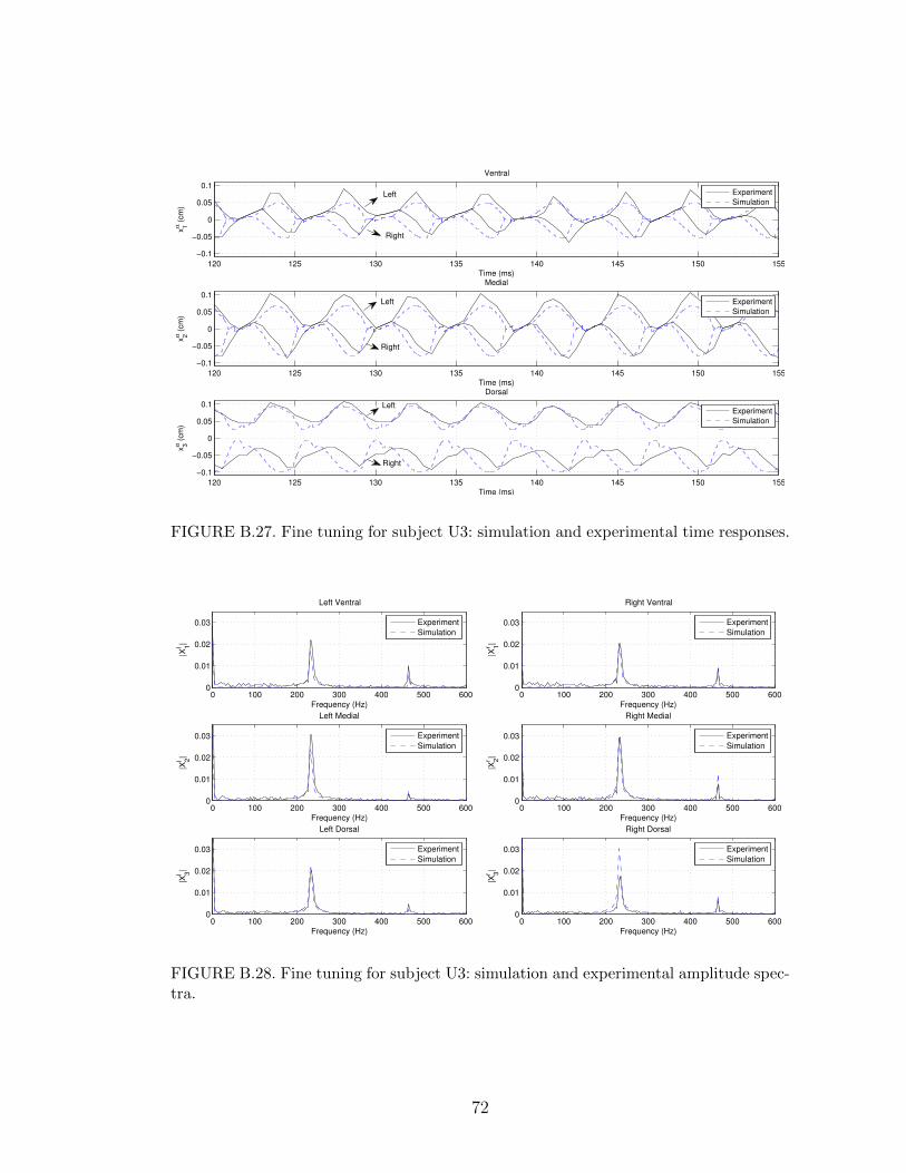
120 125 130 135 140 145 150 155
−0.1
−0.05
0
0.05
0.1
Time (ms)
xα 1 (
cm
)Ventral
Experiment
Simulation
120 125 130 135 140 145 150 155
−0.1
−0.05
0
0.05
0.1
Time (ms)
xα 2 (
cm
)
Medial
Experiment
Simulation
120 125 130 135 140 145 150 155
−0.1
−0.05
0
0.05
0.1
Time (ms)
xα 3 (
cm
)
Dorsal
Experiment
Simulation
Left
Right
Left
Left
Right
Right
FIGURE B.27. Fine tuning for subject U3: simulation and experimental time responses.
0 100 200 300 400 500 6000
0.01
0.02
0.03
Left Ventral
Frequency (Hz)
|Xl 1|
Experiment
Simulation
0 100 200 300 400 500 6000
0.01
0.02
0.03
Right Ventral
Frequency (Hz)
|Xr 1|
Experiment
Simulation
0 100 200 300 400 500 6000
0.01
0.02
0.03
Left Medial
Frequency (Hz)
|Xl 2|
Experiment
Simulation
0 100 200 300 400 500 6000
0.01
0.02
0.03
Right Medial
Frequency (Hz)
|Xr 2|
Experiment
Simulation
0 100 200 300 400 500 6000
0.01
0.02
0.03
Left Dorsal
Frequency (Hz)
|Xl 3|
Experiment
Simulation
0 100 200 300 400 500 6000
0.01
0.02
0.03
Right Dorsal
Frequency (Hz)
|Xr 3|
Experiment
Simulation
FIGURE B.28. Fine tuning for subject U3: simulation and experimental amplitude spec-tra.
72
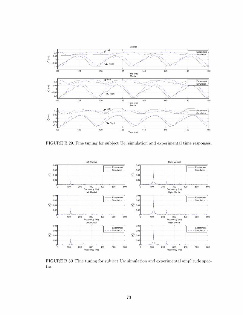
120 125 130 135 140 145 150 155
−0.1
−0.05
0
0.05
0.1
Time (ms)
xα 1 (
cm
)Ventral
Experiment
Simulation
120 125 130 135 140 145 150 155
−0.1
−0.05
0
0.05
0.1
Time (ms)
xα 2 (
cm
)
Medial
Experiment
Simulation
120 125 130 135 140 145 150 155
−0.1
−0.05
0
0.05
0.1
Time (ms)
xα 3 (
cm
)
Dorsal
Experiment
Simulation
Right
Right
Right
Left
Left
Left
FIGURE B.29. Fine tuning for subject U4: simulation and experimental time responses.
0 100 200 300 400 500 6000
0.02
0.04
0.06
0.08
Left Ventral
Frequency (Hz)
|Xl 1|
Experiment
Simulation
0 100 200 300 400 500 6000
0.02
0.04
0.06
0.08
Right Ventral
Frequency (Hz)
|Xr 1|
Experiment
Simulation
0 100 200 300 400 500 6000
0.02
0.04
0.06
0.08
Left Medial
Frequency (Hz)
|Xl 2|
Experiment
Simulation
0 100 200 300 400 500 6000
0.02
0.04
0.06
0.08
Right Medial
Frequency (Hz)
|Xr 2|
Experiment
Simulation
0 100 200 300 400 500 6000
0.02
0.04
0.06
0.08
Left Dorsal
Frequency (Hz)
|Xl 3|
Experiment
Simulation
0 100 200 300 400 500 6000
0.02
0.04
0.06
0.08
Right Dorsal
Frequency (Hz)
|Xr 3|
Experiment
Simulation
FIGURE B.30. Fine tuning for subject U4: simulation and experimental amplitude spec-tra.
73
Vita
Zhenyi Wei was born in 1978, in Zhejiang Province, China. He received a Bachelor
of Science Degree in Mechanical Engineering from Zhejiang University, China in
June 2001. He earned a master of science degree in control science and engineering
from the same university in June 2004. In August 2007 he came to Louisiana
State University and since then worked with Dr. Marcio de Queiroz as a research
assistant. He is currently a candidate for the degree of Doctor of Philosophy in
mechanical engineering.
74
Recommended