The Modelica Association Modelica 2006, September 4th – 5th
Dynamic Optimization of Energy Supply Systems with
Modelica Models
CHR. Hoffmann H. Puta
Technische Universität Ilmenau
P.O. Box 10 05 65, 98694 Ilmenau, Germany
Abstract The paper describes a design tool for decentral-ised energy supply by preferable use of renew-able energy. The powerful modelling language Modelica has been used to develop a model library for input data generation and/or predict-ing and modelling the main parts of the energy supply system for the simulation tool Dymola. An optimal control design using the well suited Dymola model in connection with Matlab [21] is performed with the solver HQP [15]. Application to a solar heating supply system with two storages demonstrates the effect of minimizing the use of additional heating and the realization by a model predictive control strat-egy.
Introduction To build a moor it needs about 50 000 years, the youngest brown coal dates from 65 million years ago, about 1850 the first coal (also oil and a bit later gas) was excavated and newest esti-mations predict that coal, oil and gas from soil may be spent in about 2250, completely. That means human activity has consumed all the natural resources developed in millions of years within a delta impulse on time scale i.e. within about 400 years! Realizing these facts it is high time that renew-able energy sources become more and more important, mainly due to the shortage of fossil fuels, which is well known. Fortunately, we still can dispose over mixed energy supply, with great challenges arising for planning and con-trol of heat supply systems, if these systems also work with different renewable energy sources (earth heat, solar radiation, exhaust air heat from building), which lead to control prob-lems with a higher rank of complexity. The main goal of these control strategies (taking into account the weather of the past and predictions of energy requirement in the future) is the re-
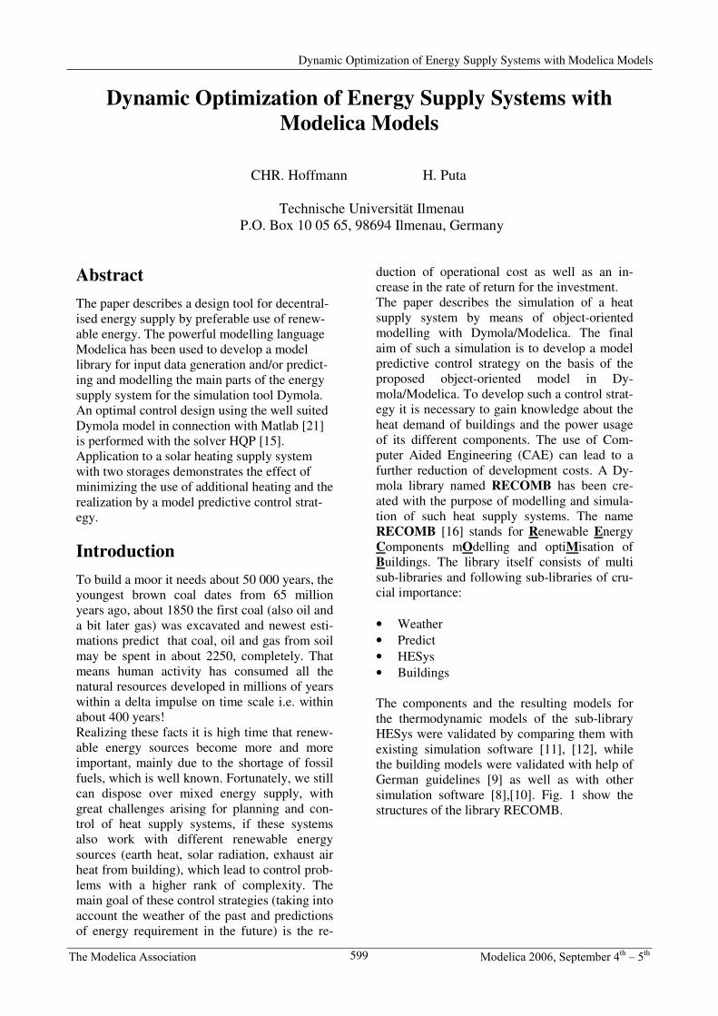
duction of operational cost as well as an in-crease in the rate of return for the investment. The paper describes the simulation of a heat supply system by means of object-oriented modelling with Dymola/Modelica. The final aim of such a simulation is to develop a model predictive control strategy on the basis of the proposed object-oriented model in Dy-mola/Modelica. To develop such a control strat-egy it is necessary to gain knowledge about the heat demand of buildings and the power usage of its different components. The use of Com-puter Aided Engineering (CAE) can lead to a further reduction of development costs. A Dy-mola library named RECOMB has been cre-ated with the purpose of modelling and simula-tion of such heat supply systems. The name RECOMB [16] stands for Renewable Energy Components mOdelling and optiMisation of Buildings. The library itself consists of multi sub-libraries and following sub-libraries of cru-cial importance: • Weather • Predict • HESys • Buildings The components and the resulting models for the thermodynamic models of the sub-library HESys were validated by comparing them with existing simulation software [11], [12], while the building models were validated with help of German guidelines [9] as well as with other simulation software [8],[10]. Fig. 1 show the structures of the library RECOMB.
599
Dynamic Optimization of Energy Supply Systems with Modelica Models
The Modelica Association Modelica 2006, September 4th – 5th
RECOMB
Buildings
Buildings
HESys
Additions
RenewableEnergy Converter
Heating
Storages
Consumer Charateristics
Weather
Power Consumption
Predict
Water Consumption
Weather
Material constants
Complete rooms
Ventilator
Wall elements
Simple Building
Heating
Heat transfer
Examples
Functions
Icons
Interfaces
Sources and Sinks
Weather
HESys
Fig. 1: Structure chart of RECOMB
This library constitutes the basic of the dynamic optimization by HQP und discrete dynamic programming by Matlab. It uses the advantage of the object-oriented modeling over the illus-tration the material flows and information flows.
Optimization In this article three different possibilities the dynamic optimization using the Dy-mola/Modelica model are shown:
1. Offline optimization by HQP and Simulink S-function interface
2. Model predictive control (MPC) by HQP and Simulink S-function inter-face
3. Discrete dynamic programming (DDP) by Matlab coupled with Dymola models via Simulink S- function interface The main goals of the different optimization possibilities are the maximization the renewable energy part to the supply of buildings and the analysis of the performance of the methods. The general continuous-time optimization problem to be solved is:
[ ] [ ])(
min),(),()())(),((0
t
t
tf
f
dtttttttIu
ux�xux →+= �ϑ
with the constrains:
[ ][ ] [ ][ ] [ ] s)constrainty (inequalit , 0),(),(
s)constraint(equality , 0),(),(
s)constraint state (final 0)(
states) (intial )(
0
0
0
f
f
f
tttttt
tttttt
t
t
∈∀≤∈∀=
==
uxh
uxf
xgxx 0
The form of this criterion is referred to as Bolza functional with Mayer term (end state evalua-tion) and Lagrange term (evaluation of the en-ergy). A first order differential equation system de-scribes the system to be optimized in the form:
( ) [ ] [ ]f,ttttttt 0 ),(),( ∈= uxfx�
The vector )(tx describes the state vector and the vector )(tu the control vector. The optimization tool HQP is a numerical opti-mal solver and before this tool can be used for the solution of the optimization problem, the problem must be discretized. The exactly dis-cretized optimization problem is shown in sub-section 3. The simple form of the general nonlinear optimization problem is:
600
C. Hoffmann, H. Puta
The Modelica Association Modelica 2006, September 4th – 5th
s)constraint
(equality 0)( and s)constraintequality
-in ( 0)( with min)(
1K
1
0
0
=
≤→
������
�
�
������
�
�
=
−
xc
xcxu
uux
x
x
eq
ineqI
�
1. Offline optimization by HQP and Simulink s-function interface
For dynamic optimization using the Dymola Modelica model the following criterion has to be maximized:
dttttuI QaEaQa HPFcum
t
t
f
)]()()([)( 3210
+−= �
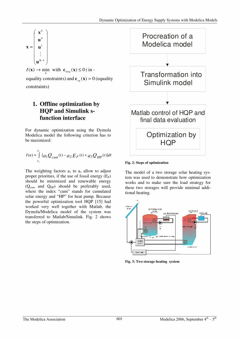
The weighting factors a1 to a3 allow to adjust proper priorities, if the use of fossil energy (EF) should be minimized and renewable energy (Qcum and QHP) should be preferably used, where the index “cum” stands for cumulated solar energy and “HP” for heat pump. Because the powerful optimization tool HQP [15] had worked very well together with Matlab, the Dymola/Modelica model of the system was transferred to Matlab/Simulink. Fig. 2 shows the steps of optimization.
Procreation of a Modelica model
Transformation into Simulink model
Optimization by HQP
Matlab control of HQP and final data evaluation
Fig. 2: Steps of optimization The model of a two storage solar heating sys-tem was used to demonstrate how optimization works and to make sure the load strategy for these two storages will provide minimal addi-tional heating.
Fig. 3: Two storage heating system
601
Dynamic Optimization of Energy Supply Systems with Modelica Models
The Modelica Association Modelica 2006, September 4th – 5th
Fig. 4: Modelica model from two storage heating system
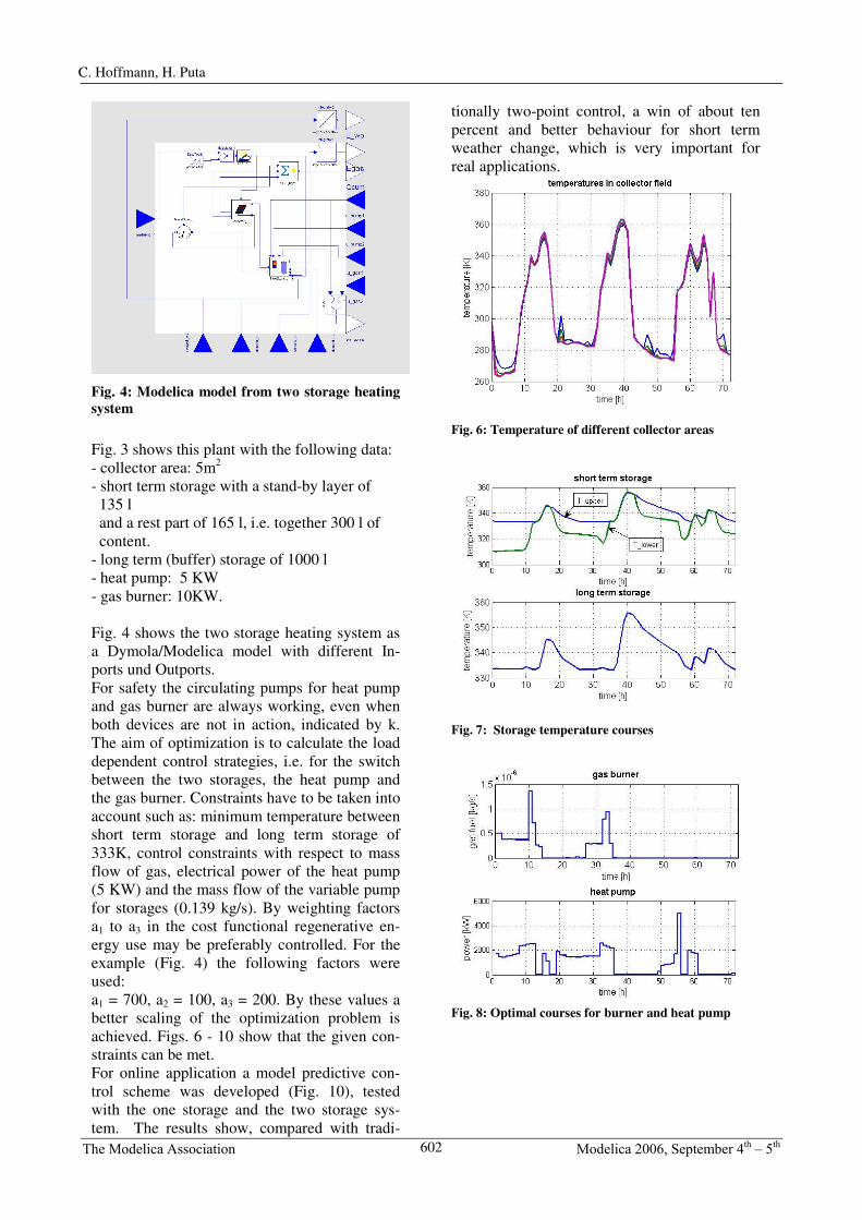
Fig. 3 shows this plant with the following data: - collector area: 5m2 - short term storage with a stand-by layer of 135 l and a rest part of 165 l, i.e. together 300 l of content. - long term (buffer) storage of 1000 l - heat pump: 5 KW - gas burner: 10KW. Fig. 4 shows the two storage heating system as a Dymola/Modelica model with different In-ports und Outports. For safety the circulating pumps for heat pump and gas burner are always working, even when both devices are not in action, indicated by k. The aim of optimization is to calculate the load dependent control strategies, i.e. for the switch between the two storages, the heat pump and the gas burner. Constraints have to be taken into account such as: minimum temperature between short term storage and long term storage of 333K, control constraints with respect to mass flow of gas, electrical power of the heat pump (5 KW) and the mass flow of the variable pump for storages (0.139 kg/s). By weighting factors a1 to a3 in the cost functional regenerative en-ergy use may be preferably controlled. For the example (Fig. 4) the following factors were used: a1 = 700, a2 = 100, a3 = 200. By these values a better scaling of the optimization problem is achieved. Figs. 6 - 10 show that the given con-straints can be met. For online application a model predictive con-trol scheme was developed (Fig. 10), tested with the one storage and the two storage sys-tem. The results show, compared with tradi-
tionally two-point control, a win of about ten percent and better behaviour for short term weather change, which is very important for real applications.
Fig. 6: Temperature of different collector areas
Fig. 7: Storage temperature courses
Fig. 8: Optimal courses for burner and heat pump
602
C. Hoffmann, H. Puta
The Modelica Association Modelica 2006, September 4th – 5th
Fig. 9: Optimal loading courses
2. Model predictive control (MPC) by HQP and Simu-link s-function interface
Fig. 10: Model predictive control scheme For the optimization with MPC-technique [19] a simple plant model with one storage was used. Fig. 11 shows this plant with the following data: - Collector area: 5m2 - short term storage with a stand by layer of 135 l and a rest part of 165 l, i.e. together 300 l of content. - gas burner: 10KW. In Fig. 10 the variables have the following meaning: x0 = x(0), initial state, used for opti-mization, xactual are the actual start values of x after some time steps, KP are forcasted climate data for starting the optimization with x0, Kactual are the actual climate values after some time steps used also as starting values for optimiza-tion. As usual the MPC (model predictive con-trol) is based on repetitive optimization, i.e. the control loop is only closed within discrete time steps to include actual data from the different sources (states, forecasts, measured data) for prediction of new optimized values (control and parameter).
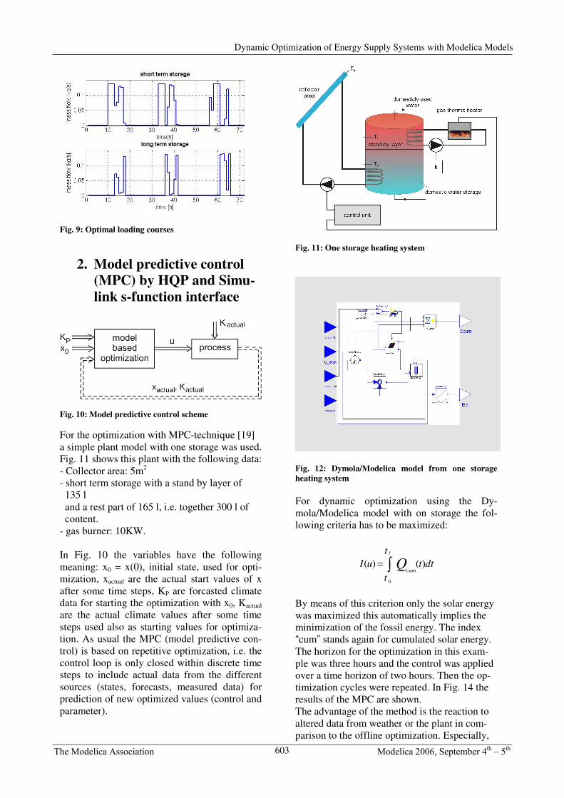
Fig. 11: One storage heating system
Fig. 12: Dymola/Modelica model from one storage heating system For dynamic optimization using the Dy-mola/Modelica model with on storage the fol-lowing criteria has to be maximized:
dttt
tuI Q
cum
f
)()(
0
�=
By means of this criterion only the solar energy was maximized this automatically implies the minimization of the fossil energy. The index “cum” stands again for cumulated solar energy. The horizon for the optimization in this exam-ple was three hours and the control was applied over a time horizon of two hours. Then the op-timization cycles were repeated. In Fig. 14 the results of the MPC are shown. The advantage of the method is the reaction to altered data from weather or the plant in com-parison to the offline optimization. Especially,
603
Dynamic Optimization of Energy Supply Systems with Modelica Models

The Modelica Association Modelica 2006, September 4th – 5th
Fig.13 shows the temperatures of the stand-by layer. Through reaction of the altered weather data with MPC-technique the limit can be met.
Fig. 13: Storage temperature courses
Fig. 14: Result courses
3. Discrete dynamic pro-gramming (DDP) by Mat-lab coupled with Dymola models via Simulink S-function interface
DDP [20] was applied to the same one storage heating system how in Fig. 11 shown in. The problem with this possibility is that the plant should not have too many states und con-trol parameters because the numbers of vari-ables increase exponentially. The problem for-mulation of the DDP is: System description:
[ ] 1,,0 ,),(),()1( −==+ Kkkkkk �uxfx Criterion with constrains:
[ ] [ ][ ][ ][ ] s)constrainty (inequalit 1,,0 ,0),(),(
s)constraint(equality 1,0 ,0),(),(s)constraint states (final 0)(
,),(),()(1
0
−=≤−==
=
+= �−
=
Kkkkk
Kkkkk
K
fixedKkkkKIK
kk
�
�
uxhuxf
xg
ux�xϑ
The calculation algorithm of the DDP [18] is divided into three parts:
1. Discretization of the considered con-tinuous problem
2. Backward calculation – one stage minimization to calculate optimal tran-sitions of the states (optimal control law)
3. Forward calculation – investigation of the optimal states trajectories and the control parameter courses from the op-timal control law.
In the following figures a comparison between HQP and DDP should be shown. The aim of the transformation from HQP to DDP is the inser-tion to build a hierarchical controller for the heat supply system for buildings on the basis of an embedded microcontroller system. Fig. 15 shows the temperature in stand-by layer of the storage and the collector field temperature. The temperature in the lower layer of the storage is similar to the collector field temperature. The differences of courses are often problems of the discretization intervals of the:
• state with x∆ and the • control parameters with u∆
between DDP and HQP. In case of DDP the discretization is bigger than in case of HQP because of a strong increase of the CPU-time.
Fig. 15: Storage temperature courses
604
C. Hoffmann, H. Puta

The Modelica Association Modelica 2006, September 4th – 5th
Fig. 16: Storage temperature courses
Fig. 17: Storage temperature courses
Conclusion As a result of this article can be said that dy-namic optimization from heating supply plants with Dymola/Modelica models is advantageous. The application of different optimization tech-niques shows the universal character of the Dymola/Modelica models. Especially the graphical programming of the plant model is of great value and it makes a relatively fast inves-tigation of control trajectories.
References [1] V. Quaschning, (1999), Regenerative Ener-giesysteme, 2. Auflage, Carl Hanser Verlag [2] Duffie and Beckmann, (1991), Solar Engi-neering of Thermal Processes [3] H. P. Garg, S.C. Mulick and A.K. Bhargava, (1985) Solar Thermal Engergy Storage, D.Reidel Publishing Company [4] Dymola User’s Manual, (2002), Dynamsin AB Lund [5] J. Kahler, (2002), Entwicklung einer Ge-bäudekomponentenbibliothek für kontrolliert-
belüftete und –entlüftete Niedrigenergiehäuser, Diplomarbeit TU Ilmenau, Inst. für Automati-sierungs- und Systemtechnik [6] M. Kisser, (2002), Entwicklung einer Prog-noseverfahrensbibliothek fuer Klimadaten in Dymola/Modelica, Diplomarbeit TU Ilmenau, Inst. für Automatisierungs- und Systemtechnik [7] W. Feist, (1994), Thermische Gebäudesi-mulation: kritische Prüfung unterschiedlicher Modellierungsansätze [8] C. Nytsch-Geusen , (2001), Berechnung und Verbesserung der Energieeffizienz von Gebäu-den und ihren energietechnischen Anlagen in einer objekt-orientierten Simulationsumgebung, Dissertation, TU Berlin [9] VDI Richtlinie 6020, (2001), Anforderun-gen an Rechenverfahren zur Gebäude und An-lagensimulation [10] F. Felgner et al., (2002), Simulation of thermal building behaviour in Modelica, Pro-ceedings of the 2nd International Modelica Con-ference [11] Solar-Institut Juelich, (1999), CARNOT Blockset Version 1.0 User manual [12] Dr. Valentin EnergieSoftware GmbH, (1999), T-Sol 2.0 User manual [13] Franke, R. (1998): Integrierte dynamische Modellierung und Optimierung von Systemen mit saisonaler Wärmespeicherung; Fortschritts-Berichte VDI, Reihe 6, Nr. 394 [14] MODELICA: Modeling of Complec Physical Systems. Modelica-Homepage. http://www.modelica.org [15] HQP: a solver for sparse nonlinear optimi-zation. Omuses/HQP-Homepage. http://hqp.sourceforge.net [16] Ch. Hoffmann, J. Kahler, Puta, H.(2003): Object-oriented simulation of energy supply systems on the basis of renewable energy. In Proceedings of the 3rd International Mode-lica conference, pp. 189-196, November 3-4, Linköping, Sweden. [17] Liu,B.Y.H. and Jordan, R.C.(1960): The interrelationship and characteristic distribution of direct, diffuse and total solar radiation, Solar Energy 4 [18] M. Papageorgiou, Optimierung, 2. Aufla-ge, Oldenbourg Verlag [19] S. Martin, (2005), Optimierte Waermever-sorgung von Gebaeuden, Diplomarbeit TU Il-menau, Inst. für Automatisierungs- und System-technik [20] T. Flemming, (2005), Optimierte Steue-rung von Energieversorgungsanlagen mit Hilfe
605
Dynamic Optimization of Energy Supply Systems with Modelica Models

The Modelica Association Modelica 2006, September 4th – 5th
der Diskreten Dynamischen Programmierung, Diplomarbeit TU Ilmenau, Inst. für Automati-sierungs- und Systemtechnik [21] Matlab: Matrix laboratory. Mathworks-Homepage. http://www.mathworks.com/
606
C. Hoffmann, H. Puta
Recommended