N79-31721 THE ECONOMIC COSTS AND BENEFITS (E79-102 6 1)
OF AN INTERNATIONAL GRAIN RESERVE PROGRAM,
ITHOUT IMPROVED (LANDSAT) CROP VITH AND Unclas A CASE sTUDY BASED ON THE ECON 1FOEMATION: 00261
(ECON, Inc., Princeton, N. G3/43INTEGRATED -ODEL
THE ECONOMIC COSTS AND BENEFITS OF AN m
INTERNATIONAL GRAIN RESERVE PROGRAM
WITH AND WITHOUT IMPROVED (LANDSAT)
CROP INFORMATION:
A Case Study Based On he ECON Integrated Model
lai-ii..'P~lIi! iL i ! i ii i
https://ntrs.nasa.gov/search.jsp?R=19790023550 2018-06-26T02:24:46+00:00Z
wy g- 1O. 2.6
77-294-1 NINE HUNDRED STATE ROAD PRINCETON, NEW JERSEY 08540
INC&PO RATED 609 924-8778
- FINAL
THE ECONOMIC COSTS AND BENEFITS OF AN
INTERNATIONAL GRAIN RESERVE PROGRAM WITH AND
WITHOUT IMPROVED (LANDSAT) CROP INFORMATION:
A Case Study Based On
The ECON Integrated Model
Prepared for
The National Aeronautics and Space Administration Office of Applications
Washington, DC
Prepared by
ECON, Inc. 900 State Road
Princeton, NJ 08540
Under Contract No. NASW-3047
December 31, 1978
i
ECONOMICS OPERATIONS RESEARCH SYSTEMS ANALYSIS POLICY STUDIES TECHNOLOCY ASSESSMENT
NOTE OF TRANSMITTAL
This final report is submitted to the National Space and Aeronautics Administration, Office of Applications, in fulfillment of Task No. 9, Contract NASW-3047. It is in two parts: (I) Final Technical Report, and (2) Summary and Overview. In addition, two separately bound Appendices (77-294-IA and 77-294-IB) documenting the computer work on the contract have been sent by ECON to the Technical Officer monitoring this task, Mr. S. Ahmed Meer at Goddard Space Flight Center.
ECON acknowledges the efforts of Philip Abram and David Lawson in usingthe ECON Integrated Model to analyze the costs and benefits of an International Grain Reserve with and without LANDSAT.
Francis M. Sand Task Manager
Bernie . Mill Project Director
ii
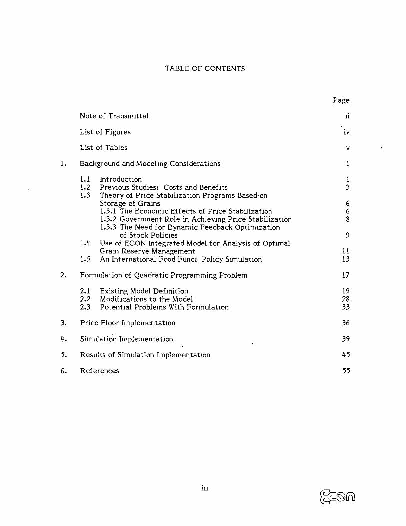
TABLE OF CONTENTS
Page
Note of Transmittal ii
List of Figures iv
List of Tables v
1. Background and Modeling Considerations 1
1.1 Introduction I 1.2 Previous Studies: Costs and Benefits 3 1.3 Theory of Price Stabilization Programs Based-on
Storage of Grains 6 1.3.1 The Economic Effects of Price Stabilization 6 1.3.2 Government Role in Achieving Price Stabilization 8 1.3.3 The Need for Dynamic Feedback Optimization
of Stock Policies 9 1.4 Use of ECON Integrated Model for Analysis of Optimal
Grain Reserve Management 11 1.5 An International Food Fund: Policy Simulation 13
2. Formulation of Quadratic Programming Problem 17
2.1 Existing Model Definition 19 2.2 Modifications to the Model 28 2.3 Potential Problems With Formulation 33
3. Price Floor Implementation 36
4. Simulation Implementation 39
5. Results of Simulation Implementation 45
6. References 55
iii
LIST OF FIGURES
Figure Page
1.1 Selected Grain Prices, U.S. Wholesale Markets 2
1.2 U.S. Stocks as a Percent of Production--30-Year Simulation 12
1.3 Price Bands for United States and ROW with International Food Fund (IFF) 15
3.1 Case I: X < QF 37
3.2 Case II: X1 < QF 37
4.1 Price Constraints on Demand Curve 40
4.2 Illustration of a Violation of the Price Ceiling 42
5.1 Simulation Model Domestic Price Series Current Versus Satellite Information System Without Price Constraints 49
5.2 ROW Price Series for 25-Year Simulations with Current and Satellite Information Systems 50
1v 9g f
LIST OF TABLES
Table Page
2.1 State Transformation Matrices for Wheat Production and Distribution 21
2.2 Incremental Value Function Coefficients 24
5.1 Comparison of an IFF with Crop Information Obtained From LANDSAT Information Systems: Initial Stocks and Present Value Costs with Two Horizons 47
5.2 Details of the International Grain Reserve Policy Simulation 51
5.3 Costs and Benefits of an International Grain Reserve with and without LANDSAT 53
v
1. BACKGROUND AND MODELING CONSIDERATIONS
1.1 Introduction
Numerous research studies have been conducted in recent years on the
economic effects of grain reserve stockpiling by the United States government,
many of them government-sponsored [1,2,3,4,5,6,7,8,9]. Some of these studies
have been collected into one volume by Eaton and Steele of USDA/ERS in
Reference 1. The essential economic goal of most grain reserve policies is price
stabilization. A secondary goal is to provide food aid when there are severe food
shortages. Price stability on domestic markets has been shown theoretically to
provide a net economic benefit to the home society, but there is controversy over
the more complicated case of a commodity which is involved in international trade,
over the distribution of benefits and over the mechanisms for achieving price
stability. Grain prices are highly variable (see Figure 1.1) due mainly to natural
variability in growing conditions which affects production. Reserve acquisitions in
times of surplus put a floor on grain prices, helping to maintain producers' income.
Release from the reserve stockpile at times of shortage puts a price ceiling on
grains, helping consumers. Methods of achieving price stability include reserve
stockpiling of grains by government, acreage controls, loans to farmers tied to
production restrictions, incentives and subsidies for private stockpiling, import/
export controls and various forms of direct price support and control policy. At
the present time, several factors tend to make a combination of government grain
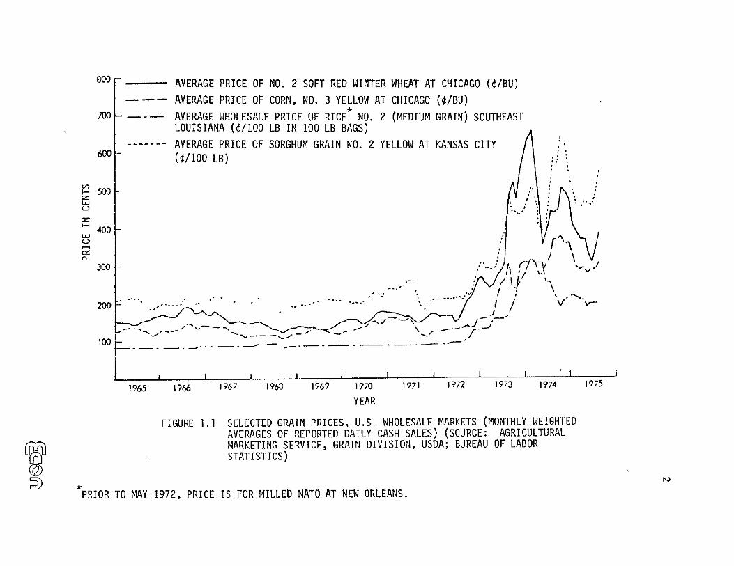
800 AVERAGE PRICE OF NO. 2 SOFT RED WINTER WHEAT AT CHICAGO (/BU)
AVERAGE PRICE OF CORN, NO. 3 YELLOW AT CHICAGO (4/BU)
700 - AVERAGE WHOLESALE PRICE OF RICE NO. 2 (MEDIUM GRAIN) SOUTHEAST LOUISIANA (/100 LB IN 100 LB BAGS)
------- AVERAGE PRICE OF SORGHUM GRAIN NO. 2 YELLOW AT KANSAS CITY 600 (€/100 LB)
-500
40
300
.......... ,ZOO ~~~ " ~ ~ . ....." ...... ... .
" " " ....
100
I I II I I I I ' I
1965 1966 1967 1968 1969 1970 1971 1972 1973 1974 1975
YEAR
FIGURE 1.1 SELECTED GRAIN PRICES, U.S. WHOLESALE MARKETS (MONTHLY WEIGHTED AVERAGES OF REPORTED DAILY CASH SALES) (SOURCE: AGRICULTURAL MARKETING SERVICE, GRAIN DIVISION, USDA; BUREAU OF LABOR STATISTICS)
rPO PRIOR TO MAY 1972, PRICE IS FOR MILLED NATO AT NEW ORLEANS.
1
reserve stockpiling and acreage controls or "set-aside" politically attractive.
'These factors include an accumulation of one of the largest U.S. grain surpluses in
history after three back-to-back record harvests.
1.2 Previous Studies: Costs and Benefits
The costs of a government grain storage program are substantial: Reutlinger
[8] in 1975 estimated that a 20-million-ton program, operated under a storage
rule that gives a high degree of protection against likely shortages, would have an
annual expected storage cost of $150 million. This program also implies, according
to Reutlinger, a net economic loss of $123 million which falls entirely on the
shoulders of the producers. The analysis m the Reutlinger paper ignores, however,
the benefits of price stabilization. An earlier 1971 study by Tweeten, Kalbfleisch
and Lu [2] found that the optimal target for wheat carryover was 400 million
bushels (or 10.9 million tons) and that the average cost of storage at this level
would be $60 million while net economic loss was $27 million at a $.20 per bushel
spread between acquisition and release prices. These figures were based on now
outdated wheat supply and demand conditions. A 1974 simulation analysis of grain
reserve stock management by Ray, Richardson and Collins [7] used the policy
New York Times Report, August 30, 1977: "Washington, August 29--In the face of mounting surpluses, President Carter has decided to curb the nation's 1978 wheat crop and give the federal government a bigger role in the grain stockpile business. The cost of the new program was estimated at $4.4 billion.
"At a White House briefing today, Acting Agriculture Secretary 3ohn White announced that the president would seek Congressional authorization for a 20 percent cutback in wheat acreage. He signaled administration intentions to get a 10 percent reduction in plantings of feed grains later in the year but said the latter decision was being delayed in case bad weather intervened.
"The program also envisages the placing of 30 million to 35 million tons of food and feed grains in reserve before the beginning of the 1978-79 marketing year. Included in the figure is a proposal to create a special International Emergency Food Reserve of up to six million tons."
4
rules of Humphrey's Senate Bill 2005 and a $.15 per bushel storage cost for wheat
to conclude that price variability would be reduced by 15 percent, and annual
storage costs would increase by $30.11 million, while annual deficiency payments
would be reduced by $85.33 million. In this study, the mean carryover of wheat
would be 483 million bushels or 13 million tons, with government stocks at 77
million bushels. Economic costs and benefits were not presented.
In modeling the welfare effects of a grain reserve policy in the much more
complicated case of a multi-national world with international grain trade, while it
is still possible to assert that the whole world gains from price stabilization [23],
it is no longer dear whether the exporting nation (the United States) gains or loses,
and whether the producers or consumers gain or lose. The nonlinearity of the
demand curve is central to this issue. Similar doubts exist for importing nations.
Hillman, Johnson and Grain [19] stated in 1975 that "(a) demand curves grown
steeper at higher prices and shallower at lower prices enhance the consumer stake
while diminishing the producer stake in reserves." Just, et al. [23] analyzed the
situation of the two-region world, one region exporting the other importing, when
the demand curve is highly nonlinear. They conclude that "producers in exporting
countries prefer (price) instability, but consumers in importing countries gain from
stabilization. Exporting countries are generally worse off and importing countries
are better off with stabilization." Since the degree of nonlinearity is shown to
affect these conclusions by Just, et al., there is clearly a need for more precise
econometric analysis of the grain demand functions, particularly in countries with
competitive markets.
In [9 ], Peter Helmberger and Bob Weaver derived welfare gains and losses to
buyers and producers in the context of a "rational expectations" model of price
uncertainty. They work with n periods--an initial period of abundance followed by
5
n-I periods of normal demand and supply. Government storage programs that
stabilize price either completely or partially are studied relative to competitive
equilibrium without government storage. Since the international gram trade is not
considered, the analysis cannot be considered "realistic." Unlike previous studies,
however, the authors do take into account the effect on private storage of the
government programs, and their conclusions differ sharply from some previous
studies [8,12] in one important respect: the net economic effect of the
government storage programs is a loss to society. Their model shows that a
massive transfer of benefits from buyers to grain producers results from a price
stabilization program based on government storage of grains.
A major recent study by the International Food Policy Research Institute
[24] considers the food security of less-developed countries which, in some years,
need to import wheat due to poor harvests. An insurance approach is employed.
Sixty-five developed countries were included in the study. Two alternative
insurance schemes were evaluated over a five-year period. The rules for release of
grains (or funds to pay for food imports) were based on the national food import bill
as a percentage of trend value (e.g., 110 percent). A percentage of projected
demand (e.g., 95 percent) is established as the target, to be maintained by the
international reserve, whenever possible. The study measures the probable cost
and the probability of maintaining the target objectives as a function of the size of
the grain reserve and the rules for operating it. An excellent feature of the study
is that it permits the costs and benefits to be treated stochastically with
understanding of the natural year-to-year fluctuation of harvests. This allows
trade-off analysis between the cost of the program and the probability of meeting
the objectives of the program. Another significant contribution which the study
uniquely provides is the disaggregation of the process of providing food security to
Over $8 billion.
6
the individual country level in the Third World. The conclusions of this research
will undoubtedly be studied closely by food program administrators and
policymakers.
1.3 Theory of Price Stabilization Programs Based on Storage of Grains
There are numerous issues, many of them controversial, surrounding the
subject of government stockpiling of grains for price stabilization or for
humanitarian food aid programs. In attempting to deal with the costs and benefits
of a government storage program here, we will focus on a few variables which have
been incorporated into analytical models by economists studying grain reserve
policy. The first is the domestic demand elasticity and indeed the entire demand
function for each specific food and feed grain, wheat for instance. The second is
the inherent variability of prices in the market system. The third is the cost of
storage. The fourth is the feedback between the market and the storage managers.
Export and import demands are also important and so is risk aversion.
The models of government storage program effects discussed here can be
classified roughly as follows:
a. Linear and nonlinear demand function
b. Trade exogenous or endogenous to the model
c. Private storage industry considered or not
d. Multiperiod versus single period model
e. Supply and demand uncertainty considered or not.
1.3.1 The Economic Effects of Price Stabilization
Economists are agreed on theoretical grounds that stability of commodity
prices conveys benefits to society [10,12,161. Hayami and Peterson [II] showed
the consumers gain, but producers lose twice that amount from a fluctuation in
7
commodity prices, given a linear demand schedule. Therefore, society would
benefit if that price fluctuation would be reduced at no cost. Subotnick and Houck
[12] analyzed the welfare implications of stabilization and showed that price
signals for government interventions were superior to quantity (production or
consumption) signals. Weaver and Helmberger [9] expressed doubt whether
quantity stabilization was feasible at all in the presence of a private storage
industry. ECON analyzed the economic benefits of price stabilization brought
about by improved crop forecasts using a dynamic welfare optimization [13, 14,
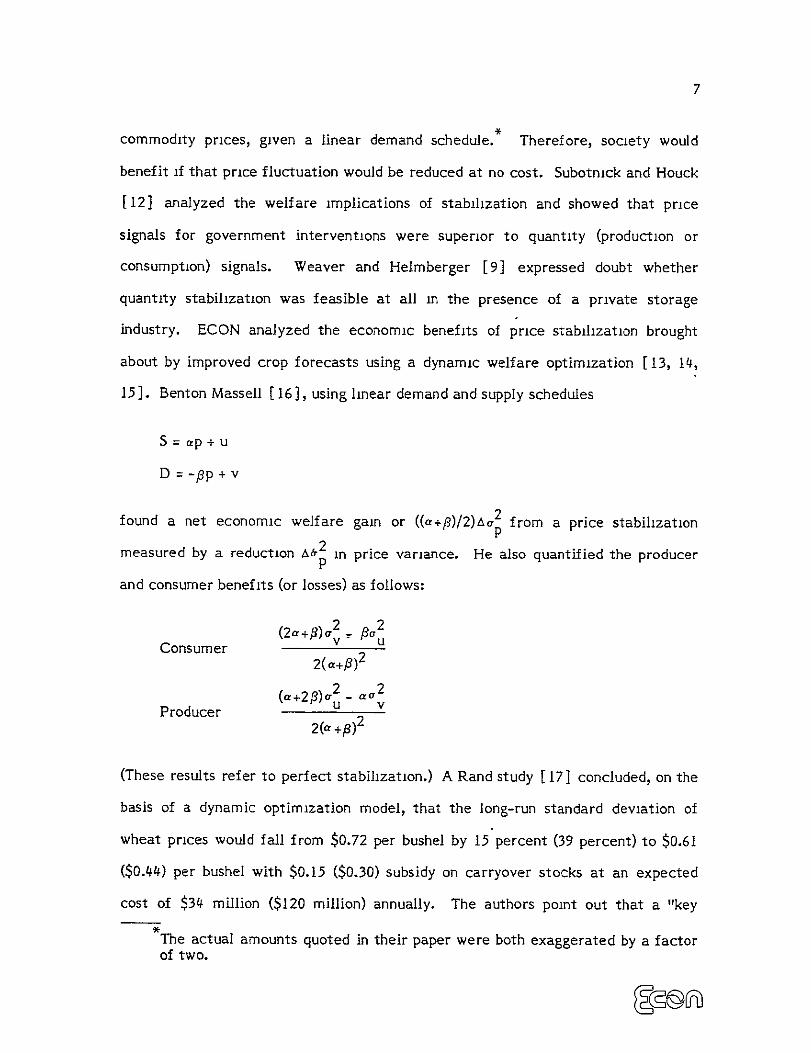
15 ]. Benton Massell [ 16 ], using linear demand and supply schedules
S =ap + u
D = -pp + v
found a net economic welfare gain or ((a+fl)/2)Ac2 from a price stabilization p
measured by a reduction A2 in price variance. He also quantified the producerirprice
and consumer benefits (or losses) as follows:
a2v ,2(2,a +,8) u2
(aPConsumer 22(a+9)
_(a+23)a 2 aa2 u vProducer
2(a +P)2
(These results refer to perfect stabilization.) A Rand study [ 17] concluded, on the
basis of a dynamic optimization model, that the long-run standard deviation of
wheat prices would fall from $0.72 per bushel by 15 percent (39 percent) to $0.61
($0.44) per bushel with $0.15 ($0.30) subsidy on carryover stocks at an expected
cost of $34 million ($120 million) annually. The authors point out that a "key
The actual amounts quoted in their paper were both exaggerated by a factor of two.
8
parameter is the rate at which government-owned grain stocks would substitute for
(and replace) privately owned stocks." This factor is overlooked in most studies,
and the consequences for evaluating government stockpiling programs are serious.
HeImberger and Weaver [9] account for private storage behavior, and show that
with a "rational expectations" approach to price uncertainty there would be
substantial gains to producers and losses to buyers from government storage
programs designed to stabilize prices. Just, et al. [23] demonstrated analytically
the importance of nonlinearity for determining even the correct signs of the
welfare effects of government price stabilization in grains.
1.3.2 Government Role in Achieving Price Stabilization
Price stability is apparently socially desirable. Why does private stockholding
not accomplish sufficient price stability? Numerous arguments have been
advanced. Briefly these include: (1) the discount rates used in evaluating private
grain storage investment; (2) risk aversion in the private storage sector; (3) lack of
competitiveness of international grain trade and grain storage markets; (4) strict
government controls in the European Economic Community, Japan and Russia
[22]; (5) producers may prefer price instability [23]; and (6) consumers may
prefer price instability [9]. But a very important reason, as pointed out in [19]
by Hillman, Johnson and Gray, is that the profit motive cannot be expected to lead
to investment in crop failures, which by their nature are somewhat unpredictable
and improbable events. Lacking more precise information, private investors will
assume an average crop, particularly at an early stage in the crop cycle when no
objective data on crop growth exists yet.
In previous ECON studies [13,14,15] we have demonstrated that improved
information on crop production worldwide would make a substantial contribution to
economic surplus in a free-market world. Given the various distortions introduced
9
into the market system by governments in their food production and trade policies,
it appeared desirable in 1977 to introduce grain reserve stockpiling by the U.S.
Government to deal with the huge surpluses, low prices and weak export demand.
Regardless of whether this policy is a good one or not, it is important to study the
impact of production uncertainty on the management of the government stocks.
We observe several points: (1) government stocks must be efficiently managed to
achieve their main purpose of price stabilization; (2) good reserve management
requires good information; (3) the secondary aim of providing international food aid
out of the government grain reserve can only be achieved if a part of the reserve is
set aside for this purpose; (4) the food aid can be more effective if good forecasts
of foreign drop failures are available in time to the administrator of this program;
and (5) the economic costs of the government grain reserve program can be
minimized if optimal acquisition and release decisions (timing and amount) are
made.
To the extent that a grain reserve goes to provide for food emergencies in
importing countries, this grain reserve will fulfill a function otherwise not met by
free trade in world commodity markets. This distinction between government
stockpiling of grains for purposes of domestic price stabilization (where stocks will
be sold on the market at some future time) and on the other hand, food aid for
needs otherwise not met (where these stocks simply "disappear" from the market),
leads to a fundamentally different assessment of effects and benefits of improved
crop information.
1.3.3 The Need for Dynamic Feedback Optimization of Stock Policies
Nearly all the grain stockpiling models which we have reviewed are either
static [8,11,23] or simulations over time in which stock levels are set by some
10
simple rule [2,3,4,7,9,24].* The models also differ on whether the production of
grains is treated exogenously or is made responsive to prices, with lags in some
cases. From our research at ECON over the past few years, we have discovered
that the consequences of ignoring the dynamic nature of the grain economy is very
serious; and that the consequences of ignoring the feedback between the market
and the grain producers and inventory holders is also serious. Gustafson [20] in his
1958 study for USDA made these same points. He developed a two-period one
world dynamic optimization model with feedback.
Johnson and Sumner [21] calculate optimal grain reserves for developing
countries and regions, using a method based on the pioneering Gustafson work.
They measure the costs of an "insurance" program for each of a number of
developing countries under which they can guarantee themselves adequate food
supplies from grain reserves when their own crops fail with a specified probability.
Concerning further work along these lines, the authors state: "Some of the most
useful generalization of this model might include the incorporation of stochastic
demands, nonindependent production probability distributions over time and
nonconstant elastic demand curves." Keeler [18] at the RAND Corporation,
seems to have developed a dynamic programming approach to optimal distribution,
although it is hard to tell from the RAND report. HeImberger and Weaver [9], in
the concluding observations of the previously mentioned paper, state: "An
important objective of this paper has been to pave the way for more meaningful
theoretical and empirical work on the efficiency and distributional consequences of
grain storage. The theoretical analysis should be extended through allowing for
changing stochastic demand and supply, risk aversion and possible externalities. *\
The latter should also be differentiated depending on whether they use a rule of thumb or an estimated behavioral rule.
11
Precise estimates of demand and supply elasticities are required for many
purposes, including the understanding of welfare effects of storage."
Taylor and Talpaz [28] present results of stochastic simulations of a first
order certainty equivalence decision rule for approximately optimal wheat stocks
in the United States. Their decision rule is obtained by maximizing a first-order
approximation of the discounted sum of expected producers' surplus plus consumers'
surplus less storage costs over a long time horizon. The methodology of their study
comes closest in essence to the ECON Integrated Model; it does not, however,
incorporate the effects of crop forecast error rates.
1.4 Use of ECON Integrated Model for Analysis of Optimal Grain Reserve Management
The ECON Integrated Model is a multiperiod, two-region world and solves the
infinite-horizon production and distribution optimization by a combination of
dynamic programming and simulation techniques. While this model was developed
to measure economic benefits of improved crop information, it is well-suited for
studying the optimal management policy for a government grain reserve.
Furthermore, because of its capability for handling the effects of crop information,
the ECON Integrated Model is valuable for obtaining an analysis of the optimal
storage program management policy under supply uncertainty; to our knowledge, no
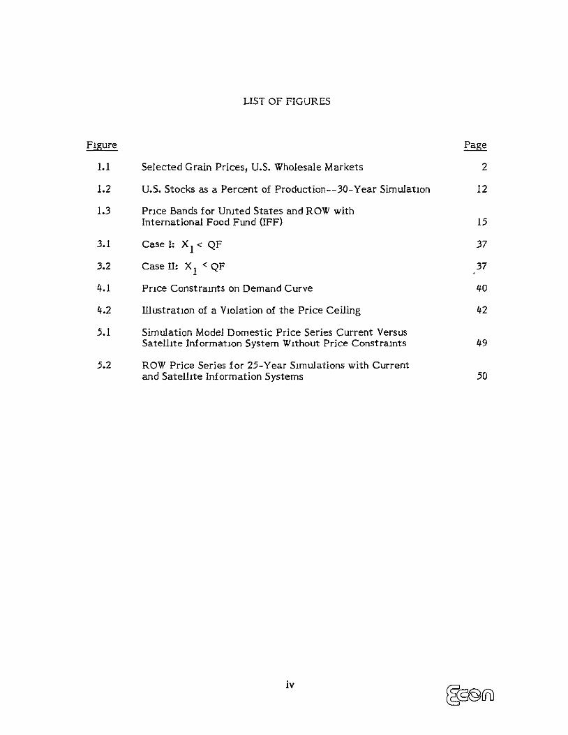
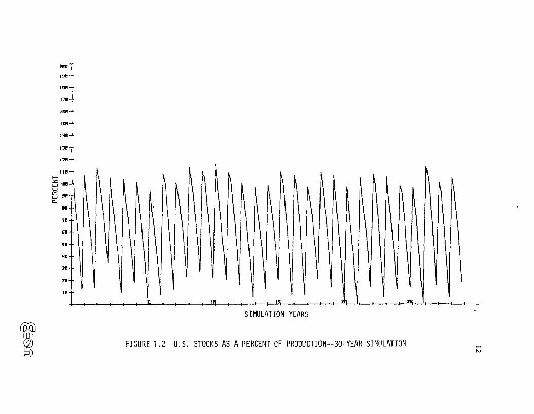
other model has this capability. Figure 1.2 shows a 30-year simulation of U.S.
wheat stocks resulting from optimal distribution decisions.
The ECON Integrated Model, with minor modifications, can be used to study
the optimal policies for U.S. grain reserve management, given various levels of
supply uncertainty (quality of crop production information). For grain price
stabilization, the optimal private storage decisions would be supplemented by
government storage of wheat for the reserve program or buffer stock. The
20T 19"±
17PI
It,
Ica..
II',I
-,
go570'
7a..
,'4
SIMULATION YEARS
) FIGURE 1.2 U.S. STOCKS AS A PERCENT OF PRDDUCTION--30-YEAR SIMULATION
13
government actions would interact through welfare optimization with the private
industry production and storage decisions.
Under price stabilization, it is assumed that the reserve will be used to
prevent excessively low prices by increased government stockpiling when there are
large surpluses, and to keep a ceiling on prices by releasing government stocks to
the market in times of grain shortage. The market price is used as a signal for
action on the part of the reserve management; government policy is to keep prices
within a specified price band. The floor and ceiling prices for this policy are inputs
to the modified Integrated Model and they act as constraints on the model's
decision making. The net economic welfare, as measured by the model's criteria, is
decreased by the policy, but the economic cost of the policy is minimized.
Under food aid programs, the aim of government policy is to provide relief to
food-deficient developing countries. Thus, grain is stockpiled to a prespecified
level (which may, however, vary as a function market price) and is released under
prespecified conditions of food shortage (high prices) in selected countries. After
release, the food aid reserve must be rebuilt over a prespecified period of time.
The rules for achieving this have a crucial effect on the economic cost of the
program, and must be specified in a clear and unambiguous manner before
optimization is possible. Once these rules are specified, the model can determine
the optimal decisions over time with respect to actual conditions.
1.5 An International Food Fund: Policy Simulation
The ECON Integrated Model has been used in this study to simulate the
operation of an International Food Fund (IFF). The sizable wheat stocks which are
acquired by the fund at the beginning are used to supply wheat when shortages
develop as signaled by high market prices. During periods of surplus, as indicated
by low market prices, the IFF replenishes its stocks, buying only sufficient wheat
14
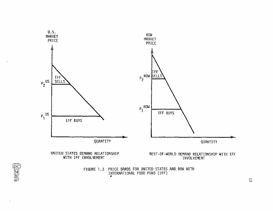
to bring the market price up to a support level. Recalling that the ECON
Integrated Model has two regions, the United States and Rest-of-World (ROW),
there are two distinct wheat markets and hence two distinct price bands to
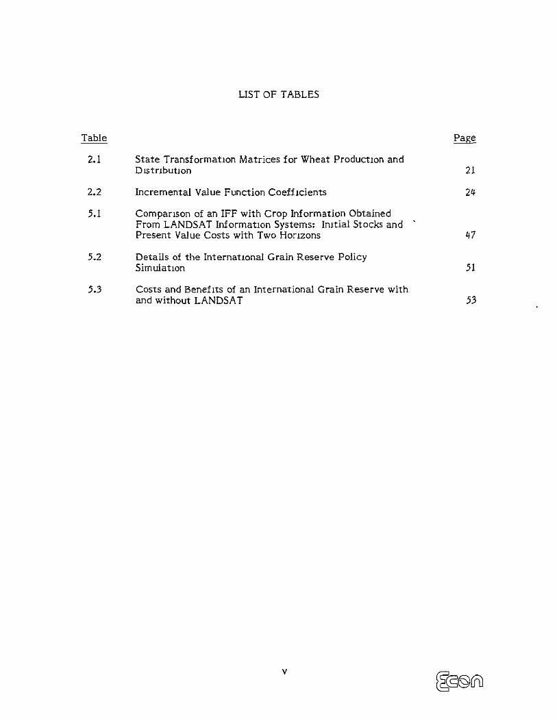
consider. The IFF in our simulation will buy and sell wheat in either market
whenever the prices trigger such actions by reaching either floor or ceiling levels
(see Figure 1.3). The wheat in the IFF stocks may be released to either region as
needed regardless of its origin. Transportation costs are always paid by importers
as in the Integrated Model itself. In effect, we have assumed that the IFF wheat
stocks are stored in the country which produced the wheat and are only transported
when needed for consumption. Most of the surpluses, of course, occur in the
United States, while most of the shortages occur in the ROW. We have not
attempted to deal with the problem of IFF financing. The initial purchase of, for
example, 27.11 MMT of U.S. wheat at a price of $140/MT requires a capitalization
of $3.795 billion. At a 15 percent annual carrying charge, such a fund has 25-year
total costs, the present worth of which under current information are $1.5 billion,
allowing for continuous purchases at $140 ($155) in the U.S. (ROW) market and
sales at $220 ($250) and eventual disposal of the remaining stocks at the prevailing
market prices. The present worth of ROW consumer benefits under current
information over the 25 years is $1.4 billion. The 15 percent carrying charge
includes storage costs of $0.625 per metric ton per month or 5 percent per annum
at average prices and interest charges of 10 percent per annum. Detailed results
are presented in Chapter 5 for various sizes of initial stocks and various price
bands.
In presenting this parametric policy simulation we are using the Integrated
Model in two ways; (1) to optimize the "free market" model for each information
U.S. ROWMARKET
MARKETPRICE PRICE
1FF 1FF P2ROW SELLS
p US SELLS
:PI ROW
IFF BUYS
QUANTITY QUANTITY
UNITED STATES DEMAND RELATIONSHIP REST-OF-WORLD DEMAND RELATIONSHIP WITH IFF WITH IFF INVOLVEMENT INVOLVEMENT
FIGURE 1.3 PRICE BANDS FOR UNITED STATES AND ROW WITH INTERNATIONAL FOOD FUND (IFF)
'a
16
system (with and without LANDSAT); output of this optimization is a set of state
variable statistics and coefficients of the steady state-value function for each
information system; (2)to simulate the IFF operations, costs and benefits over
many years, using the optimized coefficients from (1). Note, however, that the
bimonthly decisions on planting, consumption, trade and private storage are locally
optimized with respect to the fixed economic value function and state variable
statistics. There is accordingly "local feedback" from the IFF operations to the
market. For a treatment of the more ambitious undertaking of solving the
Integrated Model with IFF policy as constraints on the global optimization, see the
discussion in Chapter 2. This problem has not been fully implemented at the time
of writing.
17
2. FORMULATION OF QUADRATIC PROGRAMMING PROBLEM
In order to implement the additional constraints of a price ceiling and price
floor within the existing framework of the integrated model, several alternatives
were considered. All of the alternatives explicitly incorporated government
intervention in the form of buying and selling wheat to aid in the stabilization of
wheat prices. Two of the options seemed superior and were given further
consideration:
i. A fixed price floor and fixed price ceiling
2. A penalty cost for violating the price floor or price ceiling.
The first case occurs when the government intervenes by selling from
government stocks when the price is high and buying in the marketplace when the
price is low. The constraint allows government action only when the price achieves
the ceiling (floor) and the amount of the sale (purchase) would be strictly
determined as the amount required to exactly maintain the price ceiling (floor).
This approach shows two major weaknesses: one theoretic and one algo
rithmic. The theoretic weakness is that if the price achieves the ceiling and the
government is forced to sell, sufficient government stocks might not exist to allow
for the stabilization of the price. In this case, there is no feasible solution to the
problem without relaxing the price constraint or adjusting government stocks
artificially. In other words, some alternative action plan would be necessary since
the problem as defined could not be solved.
The algorithmic problem with the first approach is one of practicality. In the
original statement of the problem, all of the constraints on the system were linear,
A similar problem exists at the price floor.
I
thus allowing for the use of straightforward quadratic programming techniques.
The proposed first approach not only would increase the dimensionality of the
problem, but also would change the constraint set from linear to nonlinear, a
significant change in terms of the applicable solution algorithms and execution
times. Since the execution time of the model is a major consideration, and since
another viable alternative existed, the first approach was rejected.
The proposed method for implementing price stabilization constraints by
government intervention on the integrated model is to impose a penalty on any
violation of the price bounds. A severe penalty cost will imply that the bounds will
be maintained whenever feasible and a zero penalty will imply that the prices will
fluctuate as in the current unconstrained manner. By using the penalty function
approach, the two weaknesses of the first approach are avoided. For example, if
sufficient government stocks are not available for sale in case of high prices, then
the price ceiling would be exceeded and a penalty cost would be charged. The
selection of an appropriate penalty is a subject of significant interest but cannot
be fully discussed here. In addition, the penalty function can be defined as linear
and the constraint set of the expanded problem would remain linear, thus avoiding
the algorithmic weakness of the nonlinearity of the first approach.
The price constraints are to be incorporated within the existing model which
is fully described in Reference 15, particularly Chapter 4. In order to maintain
continuity in this report and consistency with Reference 15, a shortened
description of the model is presented below in which both the terminology and the
variables of the previous report will be retained. Following the discussion of the
existing model, the formulation of the modifications that would be necessary to
incorporate government intervention as price control will be described.
19
2.1 Existing Model Definition
In the model, the year is divided into six periods and export decisions are
made simultaneously with consumption versus storage decisions at the beginning of
each period. Two regions are considered, called the exporting unit (the United
States) and the importing unit (ROW). In each region, planting decisions are made
at specific times of the year, depending on the crop under study. For wheat, spring
and winter sowing are distinguished, and the Southern Hemisphere sowing occurs
half a year out of phase with Northern Hemisphere winter sowing.
State Variables
At time 1, the beginning of the first period, there are two state variables.
The first, x1 , refers to the mean value at time I of stocks in the exporting unit,
including the newly available production (still uncertain) and the carryover from
the previous crop year (known). The second state variable refers to the mean value
at time I of stocks in the importing unit. From time 1 until the start of the period
after the first planting, the same two state variables are used to track the state of
the system. At each time during this interval, x1 refers to the mean value of
remaining supply in the exporting unit, after accumulated consumption and
accumulated exports; x3 refers to the mean value of remaining supply in the
importing unit, including imports and after accumulated consumption. When the
first planting occurs in either unit, an additional state variable is created to
represent the mean value of the production expected to result from the planting in
the following crop year. Thus, there may be three or four state variables in the
middle periods of the crop year, and there will be four state variables by the end of
the crop year. When planting has occurred in the exporting unit, the new state
variable is denoted x2. When planting has occurred in the importing unit, the new
state variable is denoted x4 .
20
Decision Variables
The vector of decision variables, like the state vector, has fluctuating
dimension. There are always at least three decision variables. They are: YI'
consumption in the exporting unit; Y2 exports; and Y4, consumption in the
importing unit. In the planting periods for the exporting unit, there is also the
intended production, Y3 , and in the planting periods for the importing unit, there is
the intended production, y5.
State Transformation
The state vector undergoes a change from one time to the next as a result of
decisions and new information on existing or potential (planted) supply. The
vector Dis used to represent new information. Its elements are random variables
of zero mean. Using subscripts to indicate time, we can write the state
transformation in vector form as
Xt+1 = MtXt + NtY t + P.
The structure of Mt, Nt, and ( t' depend on the planting schedule for the particular
crop. In the case of wheat, we will model planting as occurring in periods 2 and 5
in the exporting unit (United States), and in periods 2, 5 and 6 in the importing unit
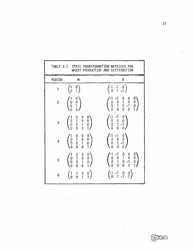
(ROW). For this case, there are six periods, and the year begins June 1. The state
transformation matrices are as given in Table 2.1.
Value Functions
We are fundamentally concerned with a cumulative value function, the
maximization of which is assumed to govern all decision making. The gross value
associated with one period's consumption y, in the exporting unit is approximated
by the polynomial
21
TABLE 2.1 STATE TRANSFORMATION MATRICES FOR WHEAT PRODUCTION AND DISTRIBUTION
PERIOD M N
°0-1-(11) °) 2 0 1 00
0 1 0 1 0 -1I (0 0 ~ 0 0 0011i0 ) (1 1 °
0 03 0 I 00 1 01 (0 01 0
4 0 1 0 0 0 0 10 IV
(00 01 0
010 0 0 010 0
0 0100 1 010 0 \ ooo°0o 0
6 0 1 -01 1 o
22
2 acy2 + 1YI ,
and the gross value associated with one period's consumption Y4 in the importing
unit is approximated by
2 a2y4 + 02Y.
These are consistent with linear demand functions
Price= 2Y1y1 + Kl
and
Price = 2 'y24 + B2
in the exporting unit and the importing unit respectively. The transportation costs
and production costs are also approximated by second degree polynomials as
follows:
= Ty 2 +Transportation Cost y
2 2
Production Cost = 3 + "k2Y5 + 6k2Y2kIy+ klY3
Here, the subscript k distinguishes the various periods within the year. The net
incremental value function for period k now can be written
23 F(yl Y2 Y 4 Y +2 2
1'y y)y,2 4 c~ 1 + ~ 1 +a 4 + 2)4 - 'Y2 '2 2 2
- YklY3 - 6klY3 k2 -ak2Y5.
Algebraically, we denote the six incremental value functions described in
Table 2.2 Flk, F 2 k, .... F6 k, where k is the period of the year. These functions can
be expressed in terms of coefficient matrices as follows:
Fik (Y) = Y'AikY + Y'Bik (2.1)
where Aik are 5 x 5 matrices and Bik are vectors of five components. These
coefficients are collected in Table 2.2.
The fundamental cumulative value function at time t, which is the discounted
sum of FIk'S, k > t, will be denoted V it The auxiliary value functions, associated
with F2k, .... F6 k, will be denoted V2t, ..., V6 t. Each is approximated by a second
degree polynomial in Xt, as follows:
Vit(Xt) = Xt QItXt + )XtLit + Kit' (2.2)
where each Qit is a symmetric matrix, Lit is a vector, and Kit is a scalar. Our
basic computational task is to find Qit and Lit , since this will enable us to
determine the dependence of Vit(X t ) on the stochastic terms $t
Dynamic Programming
The optimality principle for the system we are modeling can be written
Vlt(Xt) = max (Flt(Y) + PVl(t+l)(Xt+l ) (2.3) Y
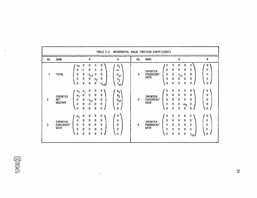
TABLE 2.2 INCREMENTAL VALUE FUNCTION COEFFICIENTS
NO. NAME
TOTAL
a 0
0 0
0
A
l0
-T 0 00
0 -YI 0 0 0 a2 0
0 0 0 -Yk2
B
-W
-kl \2
6k2
NO.
4
NAME
EXPORTER
PRODUCERS' GAIN
A
o00(oo00 0
0 0 0 0 0 0 Ykl 0 0 000 0 0
0 0 00 0
B
0
0 0
0
EXPORTER NET2WNET
a 0 0
000 O'\ 0 0 0 Oj00 \kEFR00 00
02
02 6,k10
IMPORTER CONSUMERS' GAIN
0D 0 0
00001 0 0 0 00 0
0
0 -2
0 0
o
0 0
EXPORTER CONSUMERS'GAIN
0 0 00O 00 0 0 0
60IMPORTER PRODUCERS'GAIN
000 0 0 0 0
0 O
0000
0 0 0 0 0 0 0 Yk2 0
r©
25
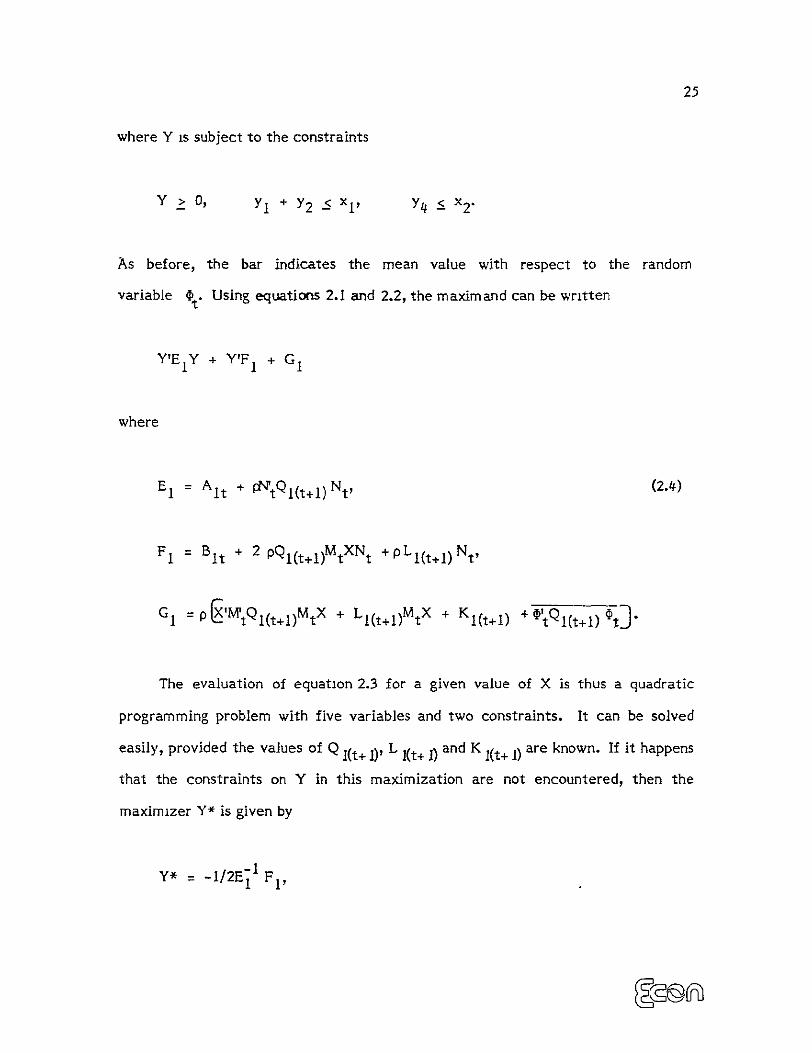
where Y is subject to the constraints
Y > 0, YJ + Y2 - x' Y4 " x2p
As before, the bar indicates the mean value with respect to the random
variable 1P"Using equations 2.1 and 2.2, the maxim and can be written
Y'EIY + Y'F + G
where
E = Ait + PtQl(t+l)Nt, (2.4)
FI =Bt + 2 pQl(t+l)MtXNt +PL(t+l)Nt,
G1 = o'-tW t+l)mt x + LI(t+l)MtX + K I(t+l) + 0 tQI(t+i) ct]"
The evaluation of equation 2.3 for a given value of X is thus a quadratic
programming problem with five variables and two constraints. It can be solved
easily, provided the values of Q I(t+ 1)' L l(t+ I)and K l(t+ I) are known. If it happens
that the constraints on Y in this maximization are not encountered, then the
maximizer Y* is given by
y* = -1/2E I F1,
26
so that V1it is a quadratic function of X. If this were always the
case, we could expand V1It explicitly in X and read off its coefficients QIt, Lik and
Kit. However, the constraints may be encountered, so Vit is not quadratic in X.
'To approximate it by a quadratic form, we select a grid of points X1, , Xn in the...
state space at time t. We evaluate V1 t at each of these points (by quadratic
programming), and then determine the coefficients Qlt, Lit and Klt of the
quadratic polynomial giving the least squares fit to Vit at the selected points. This
two-step procedure--quadratic programming followed by least squares
approximation--provides value function coefficients Qlt, Lit and Kit, assuming
Ql(t+i)' L1(t+i) and Kl(t+i) are known. At the same time, the procedure is used to
obtain the auxiliary value function coefficients Qit, Lit and K it for i = 2,... , 6,
since Vit(X) are given by
Vit(X)= Y*'EiY* +Y*FI + G
where Y* is the maximizer in equation 2.3 and
E1 = Ait + p Nt'Qi(t+i)Nt ,
Fi = Bit + 2pQl(t+l)MtXNt + PLi(t+l)Nt,
Gi =p[X'Mt'Qi(t+1)MtX + Li(t+ 1)MtX + Ki(t+ 1) + ltQi(t+1) •
Thus, the five auxiliary value functions are approximated by least squares on the
same grid as is used for VIt*
27
Starting with terminal value assumptions on Vii, i = 1, ... , 6, corresponding to
some year far in the future, we can repeat the backward induction steps described
above to obtain first Vim, i = 1 .. , th&n' Vl(m_), i = 1, ... , 6, etc. After m steps,
we obtain a new set Vim, i = 1, ... , 6, this time corresponding to one year earlier.
Continuing the cycle through the m periods each year until we get back to the
present, we finally obtain the desired functions. Because of the use of discounting,
it makes no difference what terminal value assumptions are made, provided we
begin the backward induction far enough in the future.
Another viewpoint on the same calculation is the following. Because we are
building a steady state model, the value functions should be identical at times one
year apart. Thus, for any fixed X, Vit(X) = Vi(t+m)(X) If F stands for m steps of
backward induction as described above, then we must have
rvit = Vit , i = 1, ... , 6; t = 1, ... , m.
Starting with any approximations Vt I, we can produce a sequence of approxima
tions Vit 1, Vit 2 , Vt 3 ... , by repeating r. Thus,
Vitn+l = rvitn.
When successive approximations are close enough to equal, they can be taken as
the solution of
rvit = Vit.
28
This convergence does occur in the model, because of the presence of the discount
factor p in the optimality principle (2.3).
Grid for Value Function Approximation
As mentioned above, a grid of points Xl, ... , Xn is selected in the state space
for each time t, t = I, ... , m. Initially, these grid points are selected by judgment,
so that the points cover the expected range of variation of the state vector. After
solution of the optimality principle (equation 2.4), we can explicitly evaluate the
state transformation, and thus track the development of the state vector through
many years. Using Monte Carlo simulation, we find the probability distribution of
the state vector for each time t. Then we adjust the grid points to conform to this
distribution, and repeat the procedure. This sequence--solution of optimality
principle followed by simulation--is continued until convergence is attained.
At a given time t, the grid represents a discrete eqLuprobable distribution. If
d is the dimension of the state space at time t, and n is the number of values of
each coordinate represented in the grid, there are nd points in the grid. In each
coordinate, the values are equally spaced. Such a grid is completely determined by
the mean and standard deviation of each coordinate. Thus, only these statistics are
collected from the simulations and convergence is considered to be achieved when
the means and standard deviation of each coordinate at each time of year have
stabilized.
2.2 Modifications to the Model
The constraints which are to be added to the model take the following form:
Let
PF = price floor
PC = price ceiling.
Then the desired constraints on domestic wheat prices are
E@®@
29
PF <Price <PC.
Since the price is defined as
Price = 2at1 Yl + l
then, in terms of the model, the constraints become
2a 1 Y1 + I1<PC (2.5)
2a 1 Yj + I4> PF. (2.6)
If we define two "slack" decision variables 5,1 52 as
0 <51 = amount below the price ceiling
0 < S2 = amount above the price floor
then the inequalities (2.5), (2.6) become
+2a 1I yl + a, S1 PC (2.7)
2aI Y + 81 - S2= PF. (2.8)
Since the intent of the formulation is to allow the constraints to be violated
at some linear penalty cost, then we introduce two additional decision variables
0 < V, = amount above the price ceiling
0 < V2 = amount below the price floor.
Given V1 and V2 , equations (2.7) and (2.8) can be rewritten as
2al Yl +81+ SI - VI = PC (2.9)
2aI Yl + 81 - S2 + V2 = PF. (2.10)
If the unit penalties for violating the respective constraints are defined as
30
III = unit penalty for violating price ceiling
112 = unit penalty for violating price floor
then the total associated penalty cost would be
Penalty Cost = I1 V1 +11 2 V2 . (2.11)
Since equations (2.9), (2.10) and (2. 11) are all defined in terms of prices, it is
necessary to translate the prices into quantities of wheat in order to incorporate
government buying and selling as a price stabilization control. After some minor
algebraic manipulation, equations (2.9) and (2. 10) become
I I (PC- ) (.
I 1 (PF- Bl)
Y 2 1 $2 + 2 V2 =- (2.13) 1 1
Now I V1 and V2 are the quantities below the quantity floor and above
the quantity ceiling and consist of government transactions plus violations in
excess of government transactions. Let
0 < Y6 = government sales from stocks
0 < Y7 = government purchases into stocks.
Now
Y6 -a'I V
<I1
Y7 V2
or
lV (2.14)Y6 - I + 53 =0
31
+ 54 =Y7-1 V2 (2.15) 1
where S3 , S4 are nonnegative slack variables representing the constraint violations
in excess of the government transactions with respective costs 113 and H4. Since
the government sells at the price ceiling and buys at the price floor, the associated
cost of equations (2. 14) and (2.15) is
+-PC * Y6 + PF , Y7 11 1 V1
+ 12 V2 + 13 S3 44 54"
=For simplicity we can assume 11 ]42 1 ITwhere I is a very high penalty
cost.
Notice that since
I = IY6 + S3 2 3 V-I"72- 1V a Y6
or
Y725 + = 1 1V24S= V2 -y 7
the penalty costs are double counted as
-PC • Y6 + PF Y7 + 1RV 1 +] V2 + -y 6 )+T( 2- V2 -y 7)
or )+ V2 11(1+) )
+ V 11(I + 1+ I-fI7+y6(]n-PC) + y7 (+PF)
I or
y6 (r[-PC) + y7(]+PF) + (V1 +V2 . (1 + 2ci).
The value of the objective function must be adjusted after the optimization to
adjust for the artificial penalty costs
) ] . II[y 6 + Y7 + (V1 + V2)(1 + 1 2aJ
32
In order to avoid any inconsistencies in the problem definition, we must
restrict government sales and purchases to be within some feasible region. That is
to say, government sales must be less than or equal to government stocks and
government purchases must be less than or equal to existing stocks (which includes
newly available production and the carryover from the previous year) minus
consumption minus exports. Let
0 < X 5 = government stocks.
Then
Y6 < X5
X 1 - Y 1 - Y 2 Y71X
or
Y6 < X5
Y1 +Y 2 +Y 7 -<X1
by adding slack variables, we get the equations
Y6 + S5 = X5 (2.16)
Yl + Y2 + Y7 + S6 = X1 " (2.17)
Now combining the entire constraint set we have
Yl + Y2 + $7 = 1 (2.18)
y4 + 8 =X 2 (2.19)
=Y1+ 1 $ 1 V (PC- (2.20)
Yl- IS 2 1 V2 =- 1) (2.21)YI- 22T1 2 2a
2- 16 V +S5 3 =0 (2.22)I
33
V2 + S4 0Y7- (2.23)
Y6 + S5 = X5 (2.24)
Yl + Y2 + Y7 + $6 - 1 (2.25)
and the state transformation f or X5 would be
xt+I1 t ti-I t+lX5 = X.5 + y6 - y 7 (2.26)
The incremental value function would now be
lYl 2 1+ 2 + 2Y4- y+ayl 1 Ty2 2 wY 2
YklY32_ 6 klY3 - 'k2Y52 - 6k2Y5
- PC * Y6 + PF 0 Y2 + 1I(V 1 + V2 + S3 + S4)*
In terms of the total model modification, the number of decision variabl&s goes
from 7 to 17 and the number of constraints goes from 2 to 8, a considerable
enlargement of the problem.
2.3 Potential Problems With Formulation
The primary problem with the model as presented in Section 2.1 is that the
computer time necessary for convergence is large, thereby making numerous
sensitivity runs impractical. In fact, the model which was originally programmed
using the language APL was translated into FORTRAN in order to reduce the
execution time and associated costs. Although the costs of the FORTRAN version
are significantly less expensive than the costs of the APL version, the execution
time of the model remains the major system constraint.
As discussed in Section 2.2, three.major changes would be made to the model:
(1) the state space would increase from 4 to 5, (2) the constraints would increase
34
from 2 to 7, and (3) the decision variables would increase from 7 to 17. Currently
the state space is approximated by three values in each dimension so that the
existing model has
34 = 81
grid points. If the same number of values in each dimension is maintained in the
proposed modification, the number of grid points will increase threefold to
35 - 243.
This would imply that the number of evaluations would be increased threefold in
the dynamic programming and the computer time would increase similarly.
The current algorithm used to solve the quadratic programming problem
requires a tableau of the size
Nunber of rows = NDV + NC
Number of columns = 2 - NDV + NC
where
NDV = number of decision variables
NC = number of constraints.
Thus, the size of the tableau in the current model is 9 x 16, whereas the size of the
tableau using the proposed modification is 24 x 41, an increase of more than sixfold
the number of entries in the tableau. Thus, the quadratic programming algorithm
which is in the center of the simulation will be enlarged significantly, thereby
increasing the necessary computer time.
It is dear from the above discussion that the implementation of price bounds
by government intervention is dearly a feasible project. The major drawback is
the expected increase in the computer resources that would be necessary to fully
implement the model changes. With further optimization of the FORTRAN code,
it is expected that the full implementation will be a reasonable task. Currently the
Eg @2
35
work is beyond the scope of the existing project and several more simplified
alternative implementations were considered. In the following sections, two of the
alternatives are discussed.
36
3. PRICE FLOOR IMPLEMENTATION
The desired price constraints are of the form
price floor < price < price ceiling
or
PF <2al Y + 81 <PC.
By algebraic manipulation (recall a I <0) we get
PF-S 1 Pc-S 1QC= Y1 > - =QF
or we translate the price constraints into quantity constraints where
QC = quantity ceiling
QF = quantity floor.
Avoiding the question of government intervention, we can assume that the
price constraints can be directly translated into quantity constraints as follows
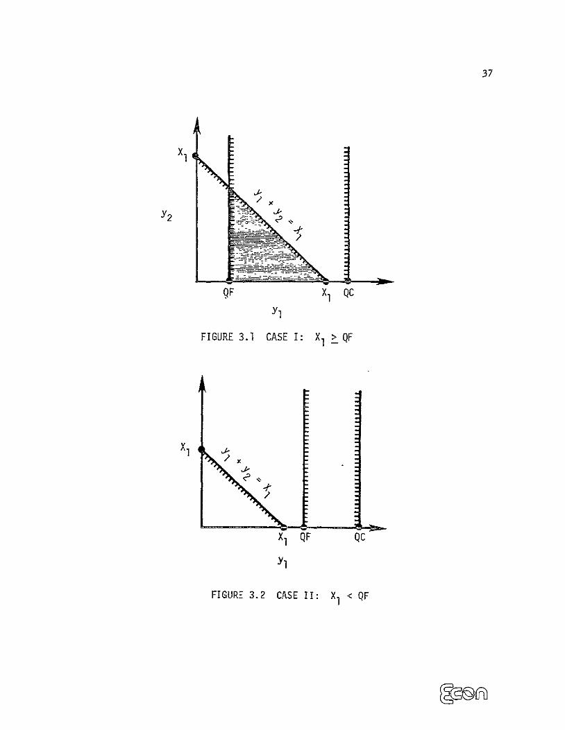
QF<y 1 <QC. (3.1)
The major problem with directly implementing this constraint (3.1) is whether it is
considered with the existing model constraints. From Section 2.1 we know that the
only other constraint involving yl is
Yl + Y2 c X1 " (3.2)
Graphically, we can see that there are two cases of interest for the feasible region
on y,, the case when X, > QF and the case where X, < QF. Figure 3.1 shows the
case when X > QF. Notice that the feasible region of y, is the shaded triangle
and the statement of the problem is consistent. The problem arises when X < QF
and Figure 3.2 illustrates the constraints. Notice that there is no region which
37
xl
-
QF
FIGURE 3.1
X QC
Yl
CASE I: XI > QF
X1 ,.
FIGURE 3.2
X, QF
Yl
CASE 1F:
QC
X < QF
38
satisfies both (3.1) and (3.2). Thus, there is an inconsistency in the problem and a
theoretic infeasibility in the problem definition.
In both of the above cases the quantity ceiling did not adversely affect the
outcome of the feasible region. In fact, there is no value of the quantity ceiling
other than zero which would cause an infeasibility. Thus, the implementation of a
quantity ceiling, which implies a price floor, does not present any conceptual
problems. The question arises, however, of whether the quantity floor (price
ceiling) would ever cause the infeasibility as shown in Figure 3.2. In virtually every
test of the model, and given a reasonable price ceiling, it was found that, in
practice, the problem becomes infeasible a significant number of times to cause
concern.
Since the price floor is the price bound of the most interest and since it
relates to the 90 percent parity demands of farmers, a version of the model was
created which implemented only the price floor
constraint is implemented in the model as the quantity
constraint.
constraint
In effect, this
Y1 <'
PF- 61
-
thereby increasing the size of the quadratic programming tableau from 9 x 16 to
10 x 17 and not changing the number of decision variables. This version is available
but sufficient runs have not been made to determine the effect of the constraint on
the value function.
39
4. SIMULATION IMPLEMENTATION
The'most straightforward implementation of the model with government
intervention is that of including government actions only in the final simulation,
after the value functions have been documented. The simulation is run in the usual
manner and the government transactions are recorded parallel to the model. The
value function coefficients are those obtained in the convergence process of the
model without the grain reserve program. Thus, the quadratic, linear and constant
terms of the objective function in the optimization are those obtained in a free
market economy and do not incorporate the changes that would be a result of
government intervention. The primary inputs of the simulation runs are the value
function coefficients and the initial state values of X1, the mean value of
remaining supply in the exporting unit, and X3, the mean value of remaining supply
in the importing unit.
The form of the constraints in this implementation is
price floor < market price < price ceiling.
We will simplify the presentation in this section by referring only to the U.S. case;
similar equations and inequalities must be added to the ROW constraint set. Thus,
PF <2 aI Y1 l (4.1)Y+ PC
where 2a 1 and I are the slope and intercept of the domestic demand curve and y,
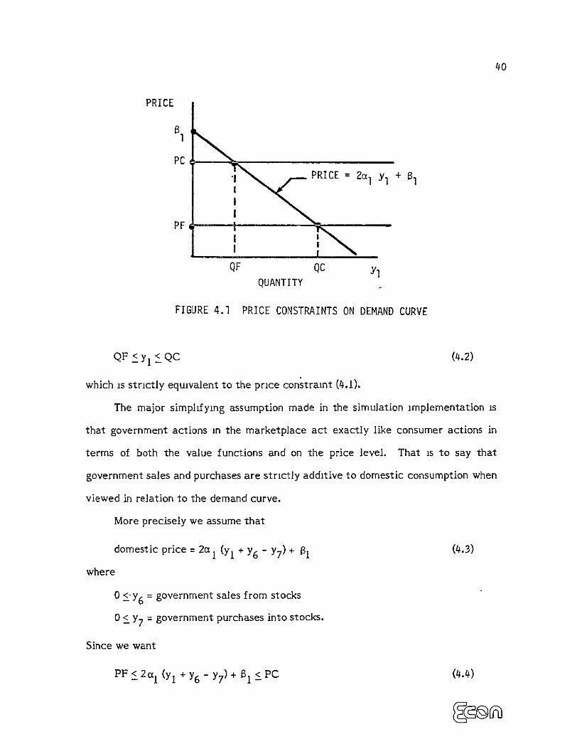
is the decision variable representing the level of domestic consumption. Figure 4.1
gives a graphical representation of the linear demand curve and the price
constraints. Notice that the price ceiling implies a quantity floor and that a price
floor implies a quantity ceiling. Thus, we wish to constrain consumption as
40
PRICE
B
PC +'IPRICE 22 I Yl
PF
QF QC Yl QUANTITY
FIGURE 4.1 PRICE CONSTRAINTS ON DEMAND CURVE
QF <yl <QC (4.2)
which is strictly equivalent to the price constraint (4.1).
The major simplifying assumption made in the simulation implementation is
that government actions in the marketplace act exactly like consumer actions in
terms of both the value functions and on the price level. That is to say that
government sales and purchases are strictly additive to domestic consumption when
viewed in relation to the demand curve.
More precisely we assume that
domestic price = 2a 1 (Y1 + Y6 - Y7 ) + Si (4.3)
where
O<-y 6 = government sales from stocks
O< Y7 = government purchases into stocks.
Since we want
<PF < 2a 1 (Y1 + Y6 - Y7 ) + B1 PC (4.4)
41
and since we define
=Y6 . y7 0
we will have the government intervene only when
2>I Y, + 61 PC (4.5)
or
PF (4.6)+ j <2lYl
where y1 is the optimal value of y,, as determined in the model.
The level of government action required to satisfy the price constraints
whenever either (4.5) or (4.6) occurs is now strictly determined. Consider the case
of the price exceeding the price ceiling by AP. Then
2CI Yl + I = PC + AP. (4.7)
Using (4.3) we know that
2(YI* + Y6 - Y7) + 81 = PC. (4.8)
Subtracting (4.8) from (4.7) we get
2a 1 (y7 -y 6 ) = AP
or AP (4.9)Y7"-Y6 = 2aI"
Since we know that Y6 " Y7 --0, 2a 1 < , Y6 < 0, Y7 >0, AP > 0 we determine that
(4.10)Y6
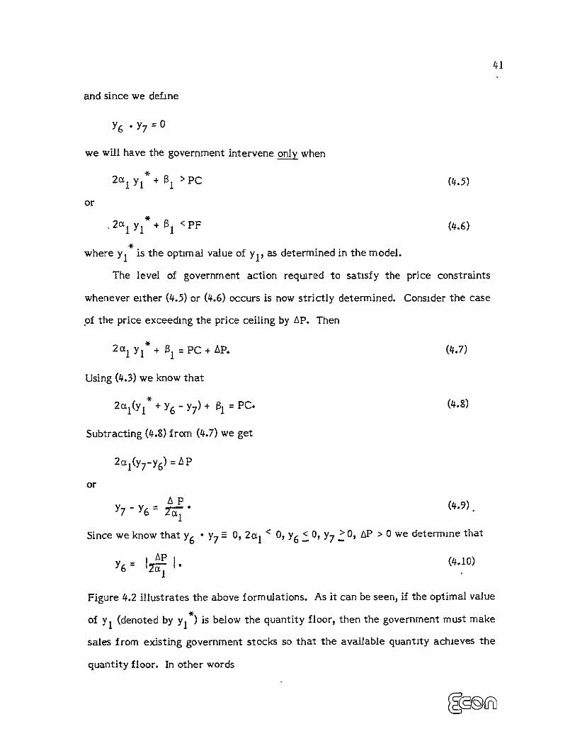
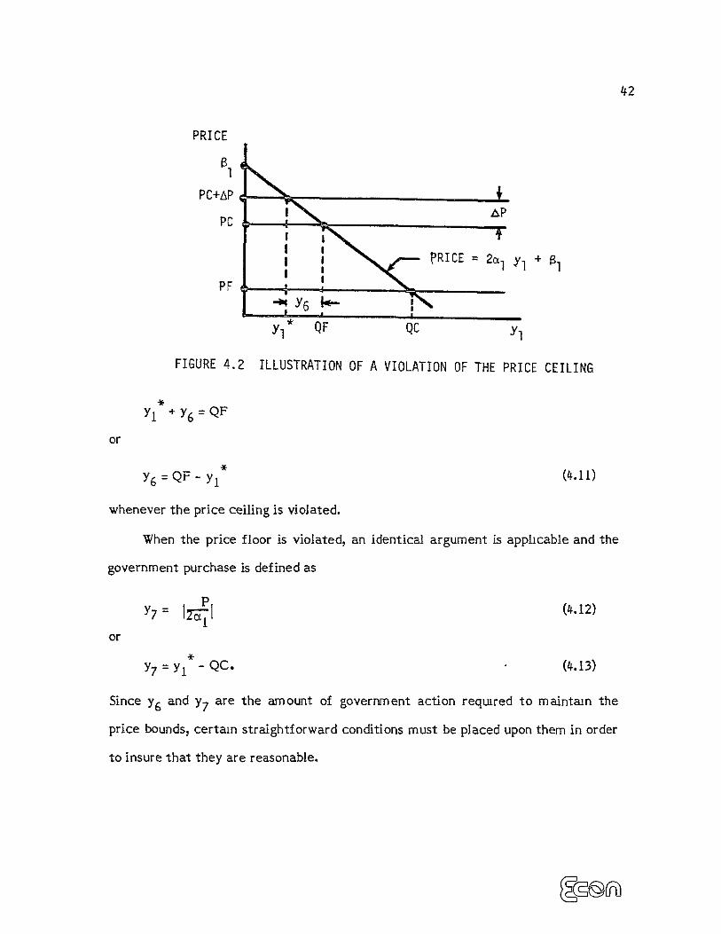
Figure 4.2 illustrates the above formulations. As it can be seen, if the optimal value
of Y1 (denoted by y1*) is below the quantity floor, then the government must make
sales from existing government stocks so that the available quantity achieves the
quantity floor. In other words
42
PRICE
S
PC+AP I AP
PC
PRICE = 2 1 Yj + l
PF I
U I
Y t QF QC Yl
FIGURE 4.2 ILLUSTRATION OF A VIOLATION OF THE PRICE CEILING
Y1 +Y6 QF
or
Y6= QF - yl (4.11)
whenever the price ceiling is violated.
When the price floor is violated, an identical argument is applicable and the
government purchase is defined as
Y7 = Il (4.12)
or Y7 = Y - QC. (4.13)
Since Y6 and Y7 are the amount of government action required to maintain the
price bounds, certain straightforward conditions must be placed upon them in order
to insure that they are reasonable.
43
The first constraint is that the government'sales are less than or equal to the
existing government stocks. In order to implement this constraint, an exogenous
variable must be added to the system as
0 < X5 = level of government stocks.
We assume that if sufficient government stocks are not available to reduce the
price of the price ceiling, then all existing stocks are sold and the price constraint
remains violated. A sufficiently high initial level of government stocks will insure
that the above infeasibility never occurs. Thus we want
Y6Z (4.14)5
The second constraint is that government purchases cannot exceed the
existing supply on the marketplace. Thus,
- y -Y7 -I Y2
or
< X I yl + y7 Y2
where Y2 is the export of wheat. In other words, government purchases plus
consumption has to be less than the existing supply minus exports.
A state transformation is required for the exogenous X5 and is defined as
y6t+! 5t+l =5xt - y7t+l
or the government stocks of the current period are the government stocks of the
previous period minus government sales plus government purchases. Since the
government transactions affect the existing supply, the state transformation for
X I must be altered as follows
t + ! _xl1t+I = X lt - y _ y2t+ I-+ y6t + l y7 t + 1
44
In other words, all government transactions come from and go to the existing
supply. This is the only way in which the government intervention simulation
implementation impacts the existing model.
For an international grain reserve, the implementation requires four distinct
transactions.
1. Initial purchase of stocks
2. Purchases to maintain price floor
3. Sales to maintain price ceiling
4. Disposition of remaining stock at end of simulation.
The assumptions of the transactions are as follows. The initial purchase of grain
reserve stocks is made at the initial period at the current market prices prevailing
in both regions. The initial level of stocks is an input parameter which can be
varied for sensitivity analysis. All purchases are made at the price floor. All sales
are made at the price ceiling. At the end of the simulation, the remaining stocks
are sold at the existing market prices prevailing in the region where the stocks are
held. These costs are tracked over the period of the simulation and a total
discounted present value of grain reserve costs is the primary output. Since the
present value includes the purchase of the stock in the initial period and the future
transactions are discounted, the present value will always be negative.
45
5. RESULTS OF SIMULATION IMPLEMENTATION
The International Food Fund (IFF) simulation model as described in
Section 1.5 was implemented in FORTRAN on the Princeton University IBM
370/158 computer. The converged value function coefficients were obtained from
the ECON Integrated Model. Several parametric runs of the programs were made
to determine the overall behavior of the IFF simulation model, The parameters of
most interest for analyses were the respective values for the price bands for the
United States and ROW and the starting IFF stocks. The simulation was run
through a 50-year period for several alternative combinations of price bands and
starting stocks with both current and LANDSAT information systems. The
information systems were given the same performance measures used in previous
ECON benefit/cost studies [ 15]. LANDSAT performance evaluation is based on
the General Electric Sigma Squared Study [29].
The principal outputs from the model were the present value of the IFF cost
to maintain the stocks, and the present value of world (U.S. and ROW) benefits
from the fund. Since the costs of the transactions were discounted, the dominant
cost appearing in the present value calculation in case of significant starting stocks
was the purchase of an initial inventory. This initial inventory was set at such a
level that the fund would only just not run out at any time in the 50 years so as to
fulfill the policy goals at minimum cost. Final residual stocks in IFF were sold off
at prevailing market price after 50 years. The IFF initial purchases and final sales
were not allowed to affect prices. While somewhat unrealistic, this assumption has
very little effect on the character of the results.
46
The length of the simulation runs--50 years--was chosen after determination
of the sensitivity of the present value of the discounted stream of benefits to run
length. It was found that significant changes in this quantity occurred after 25
years, but that it was insensitive to increased run length beyond 50 years. As a
consequence of the long horizon implicit in our policy simulation methodology, the
required initial IFF inventory was rather large. In future work it would be
desirable to simulate a more conservative policy; for example, one which allows
replenishment of the IFF inventory outside of the price band every five or ten
years in addition to IFF purchases made solely to support prices at the price floor.
The one case of a high ($l60/metric ton) ROW price support level had to be
rejected from the subsequent benefit analysis due to its anomalous cost indications.
The set of results used the converged coefficients of the value function with
a 15 percent rate of discount. This rate was selected to represent inventory
carrying charges--approximately 5 percent for storage costs and 10 percent for
interest. Table 5.1 presents a comparison of the costs of an IFF for several cases
of starting IFF inventory and ROW price floor, all other policy variables being held
constant.
Notice that in all of the cases except one, the cost to the fund of
maintaining the price stabilization policy is less with the LANDSAT information
system than with the current information system. The main reason for this
difference is that, with better information, the IFF can start with smaller stocks.
Since these starting stocks have to be purchased at prevailing market prices, the
IFF costs are less. In reality, a stockpile would be built up gradually out of surplus
The anomaly is due to the fact that this particular policy results in a longterm upward trend in IFF stocks which is counter to the policy goal of usingthe reserve to benefit consumers and producers.
E@2
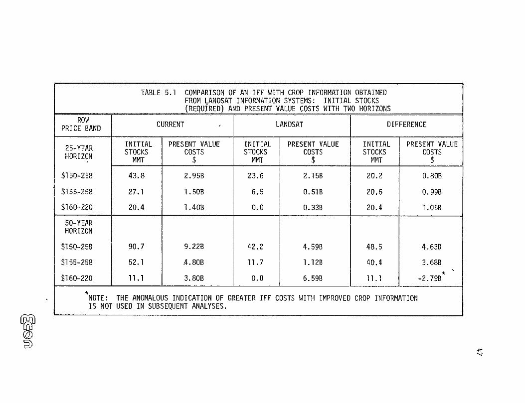
TABLE 5.1 COMPARISON OF AN IFF WITH CROP INFORMATION OBTAINED FROM LANDSAT INFORMATION SYSTEMS: INITIAL STOCKS (REQUIRED) AND PRESENT VALUE COSTS WITH TWO HORIZONS
PRICEROWBAND CURRENT LANDSAT DIFFERENCE
INITIAL PRESENT VALUE INITIAL PRESENT VALUE INITIAL PRESENT VALUE25-YFAR STOCKS COSTS STOCKS COSTS STOCKS COSTS HORIZON MMT $ MMT $ MMT $
$150-258 43.8 2.95B 23.6 2.15B 20.2 0.80B
$155-258 27.1 1.50B 6.5 0.51B 20.6 0.99B
$160-220 20.4 1.40B 0.0 0.33B 20.4 1.05B
50-YEAR HORIZON
$150-258 90.7 9.22B 42.2 4.59B 48.5 4.63B
$155-258 52.1 .4.80B 11.7 1.12B 40.4 3.68B
$160-220 11.1 3.80B 0.0 6.59B 11.1 -2.79B
NOTE: THE ANOMALOUS INDICATION OF GREATER IFF COSTS WITH IMPROVED CROP INFORMATION IS NOT USED IN SUBSEQUENT ANALYSES.
©
48
private or U.S. government stocks, thus reducing both IFF costs and market
impact.
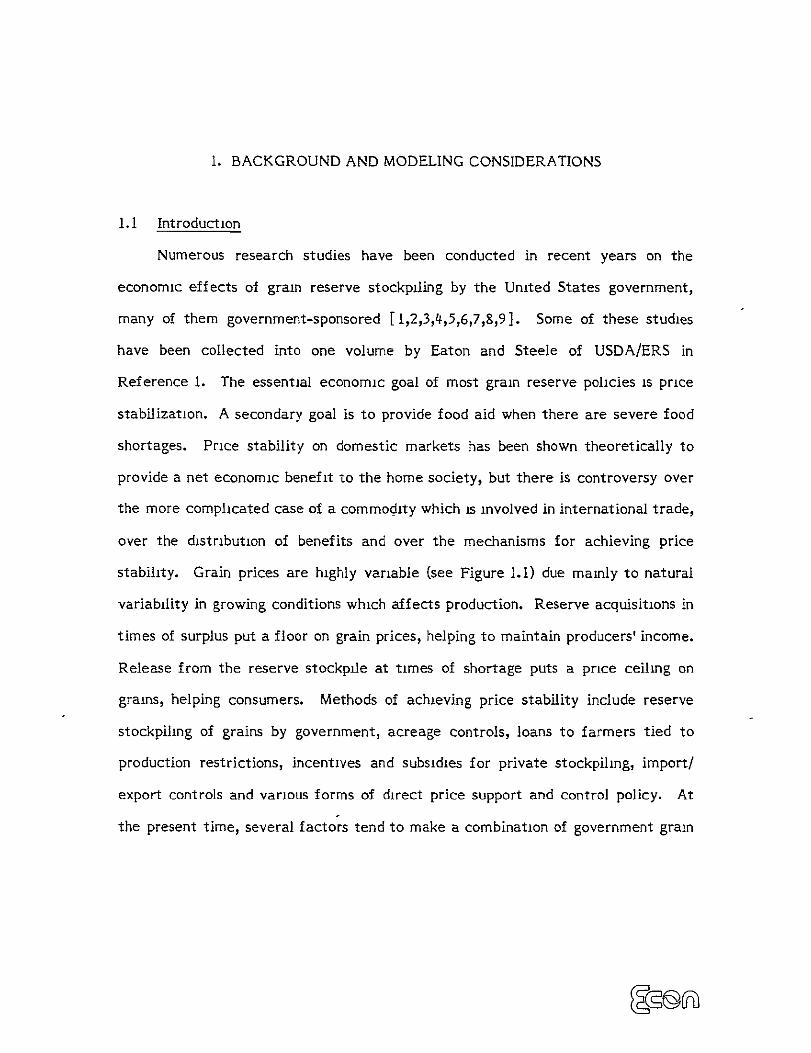
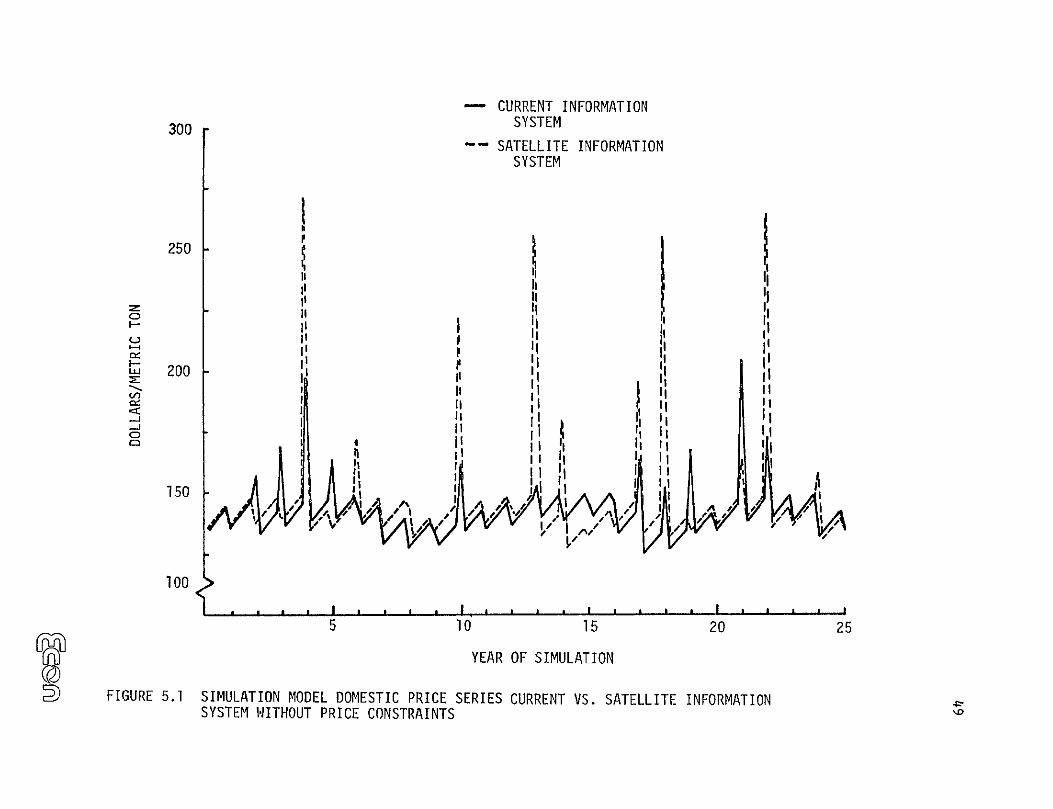
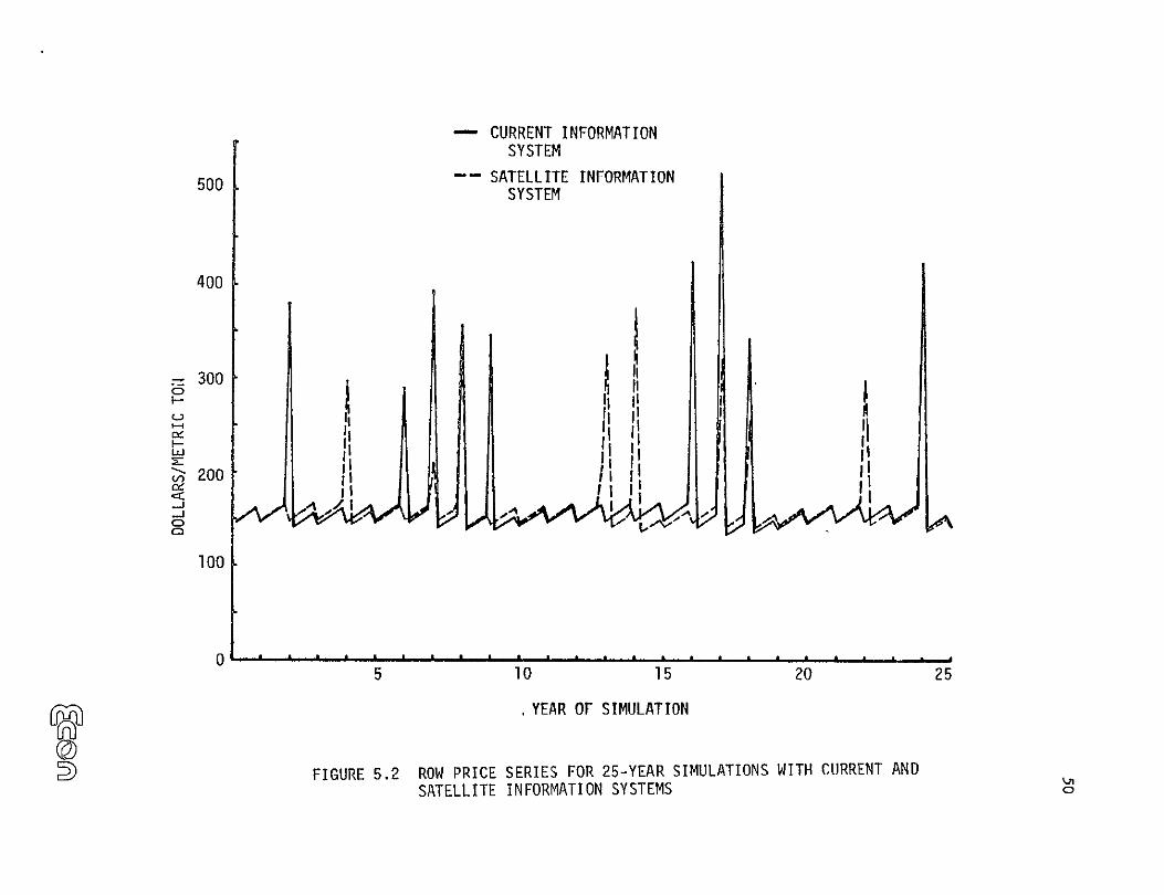
Figure 5.1 illustrates the U.S. price series (without price constraints) and
Figure 5.2 illustrates the ROW price series for both current and satellite
information systems. For both information systems, the price peaks are very sharp
and there is no comparable valley to lower prices. Since high prices occur with
undersupply and low prices occur with oversupply, these results illustrate that the
model optimization tends to reduce the possibility of oversupply. In reality, large
surpluses do occur due to bumper crops being harvested in many parts of the world.
The plot also shows that the domestic price in the satellite case tends to be, in
general, higher with approximately the same number of peaks. The major
difference in the two cases is that the magnitude of the peaks in the satellite case
is significantly larger than the magnitude of the peaks in the current information
case for U.S. prices and the reverse for ROW prices.
The second principal output variable is the per period IFF transactions and
the level of IFF stocks. For the sake of fulfilling the policy goals over many years,
the level of IFF stocks should remain approximately stable; that is to say that
there should be no long-term trend. If there were a generally increasing trend to
the level of IFF stocks, the average annual IFF purchases would be generally higher
than the average annual IFF sales. This implies that the price floor has been
violated more often or with greater magnitude than has the price ceiling. To
eliminate such a trend, the price levels of the floor and/or ceiling can be adjusted
until an equilibrium is attained in the level of IFF stocks.
Table 5.2 presents some statistics pertaining to the level of IFF stocks and
transactions for the 50-year simulation runs. The level of initial IFF stocks was
chosen so as just to avoid any stock-out during the 50-year period of the
300
-- CURRENT INFORMATION SYSTEM
-- " SATELLITE INFORMATION SYSTEM
I p
250 1P
iI II CDJ o II
I I--II ,
I- II 'I IIC- I III i
w 200 II.Ih p
° I,
I III
150
5 10 15 20
YEAR OF SIMULATION
FIGURE 5.1 SIMULATION MODEL DOMESTIC PRICE SERIES CURRENT VS. SATELLITE INFORMATION SYSTEM WITHOUT PRICE CONSTRAINTS
25
- CURRENT INFORMATION SYSTEM
500 -- SATELLITE INFORMATION SYSTEM
400
300
I-C-,
r II I i
100' 0
0 . . . ; . . o.... .. " " ' h'' ' 5 10 15 20
YEAR OF SIMULATION
FIGURE 5.2 ROW PRICE SERIES FOR 25-YEAR SIMULATIONS WITH CURRENT AND SATELLITE INFORMATION SYSTEMS
25
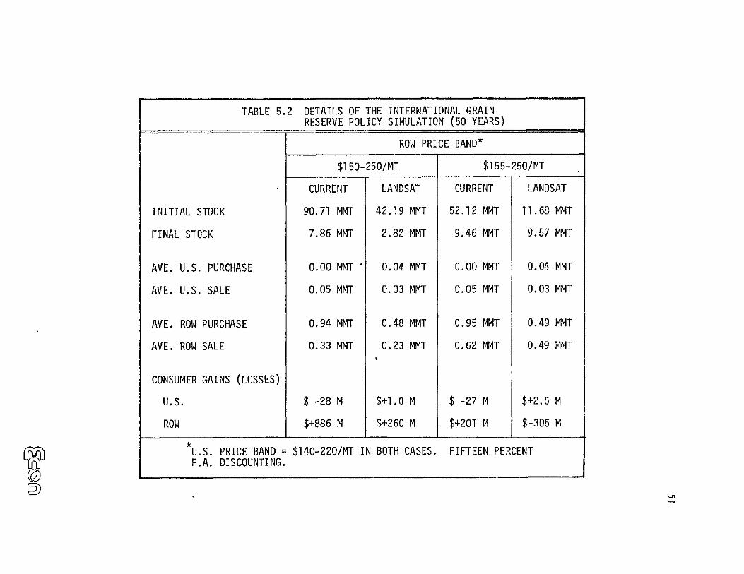
TABLE 5.2
INITIAL STOCK
FINAL STOCK
AVE. U.S. PURCHASE
AVE. U.S. SALE
AVE. ROW PURCHASE
AVE. ROW SALE
CONSUMER GAINS (LOSSES)
U.S.
ROW
U.S. PRICE BAND = P.A. DISCOUNTING.
©I
DETAILS OF THE INTERNATIONAL GRAIN
RESERVE POLICY SIMULATION (50 YEARS)
ROW PRICE BAND*
$150-250/MT $155-250/MT
CURRENT LANDSAT CURRENT LANDSAT
90.71 MMT 42.19 MMT 52.12 MMT 11.68 MMT
7.86 MMT 2.82 MMT 9.46 MMT 9.57 MMT
0.00 MMT 0.04 MMT 0.00 MMT 0.04 MMT
0.05 MMT 0.03 MMT 0.05 MMT 0.03 MMT
0.94 MMT 0.48 MMT 0.95 MMT 0.49 MMT
0.33 MMT 0.23 MMT 0.62 MMT 0.49 MMT
$ -28 M $+i.O M $ -27 M $+2.5 M
$+886 M $+260 M $+201 M $-306 M
$140-220/MT IN BOTH CASES. FIFTEEN PERCENT
52
simulation. From Table 5.2 we learn that the average U.S. net transactions of the
IFF are always larger and average ROW net transactions are always smaller
(algebraically) with satellite as compared with current information systems. Most
notable of the results of these policy simulations, however, are the dramatic
effects of (I) the ROW price floor, and (2) the improved crop information system
on the required size of the initial IFF stocks. By increasing the price floor, one
induces ROW to supply more of its surplus wheat to the IFF, thus making it less
dependent on the initial stocks. ROW purchases from the fund are not much
affected by this variable. On the other hand, the improved information system
drastically reduces the ROW need for IFF buffer stocks; both the size of the
starting IFF stocks and the average ROW transactions are reduced. This result
reflects in a quantitative way the trade-off between wheat buffer stocks and crop
information which has been discussed speculatively in the past.
The extent to which the fund creates benefits depends on the rules of its
usage. In analyzing the benefits, it is important to remember that the IFF must
purchase wheat from the regional markets when prices are low as well as selling
wheat in times of shortage at higher prices. When wheat is purchased by the fund,
prices are driven up, creating a consumer disbenef it. Thus, the benefits of IFF
releases at relatively high prices are offset, to some extent, by the disbenefits
caused by IFF acquisitions. If the fund is poorly managed, or if the price bands are
not chosen judiciously, the net effect may be an economic loss rather than a
benefit. Table 5.3 presents the economic costs and benefits of an IFF with and
without LANDSAT. The economic effects of improved information due to
LANDSAT are dearly to reduce both the required starting inventory and the cost
of the IFF. At the same time, benefits are also reduced. The net effect is an
economic gain for the world if the policy is implemented with LANDSAT rather
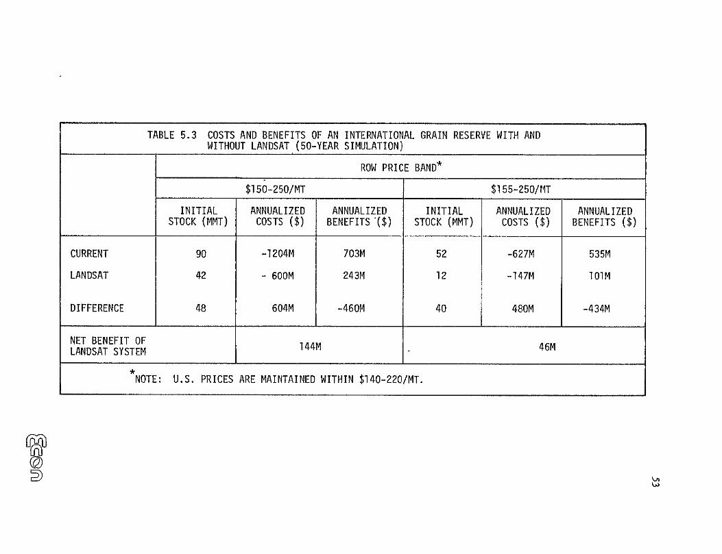
TABLE 5.3 COSTS AND BENEFITS OF AN INTERNATIONAL GRAIN RESERVE WITH AND
WITHOUT LANDSAT (50-YEAR SIMULATION)
ROW PRICE BAND*
$150-250/MT $155-250/MT
INITIAL ANNUALIZED ANNUALIZED INITIAL ANNUALIZED ANNUALIZED STOCK (MMT) COSTS ($) BENEFITS '($) STOCK (MMT) COSTS ($) BENEFITS ($)
CURRENT 90 -1204M 703M 52 -627M 535M
LANDSAT 42 - 600M 243M 12 -147M lOIM
DIFFERENCE 48 604M -460M 40 480M -434M
NET BENEFIT OF 46M144M
NOTE: U.S. PRICES ARE MAINTAINED WITHIN $140-220/MT.
LANDSAT SYSTEM
54
than with current crop information standards. This gain is $100 million per year
larger using the $150 ROW price support than it is with the $155 price support, thus
indicating sensitivity of the economic results to the choice of the IFF policy rules.
In order to analyze the effect on fund costs and benefits of the improved
(LANDSAT) information system, we select the most "reasonable" of the simulation
cases, which is the first case (price band $150 to $250 for ROW). The annualized
50-year IFF costs are reduced by 50 percent as a result of the LANDSAT crop
information, largely due to the much lower required starting stocks. However, at
the same time, consumer benefits throughout the world are reduced by 70 percent,
most of this reduction occurring in the ROW. The improvement of wheat
forecasts--specifically the reduction of forecast mean square error--in our model
achieves some of the purposes of the fund, and hence reduces the fund's potential
for benefiting consumers of wheat.
Comparing IFF costs with benefits for the same case ($150 to $250), we find
that, under current information, the benefit-to-cost ratio is 0.58, while under
improved information this ratio drops to 0.41. Using this criterion for deciding
whether or not to create a fund, it appears that one would prefer not to create the
IFF at all on strictly economic grounds regardless of the quality of the information
system. However, if the decision to create an IFF has already been made on other
grounds, the implementation of the LANDSAT information system generates
substantial cost savings which can be translated into a net economic benefit with
suitable choice of the policy rules.
55
6. REFERENCES
1. Eaton, David 3. and W. Scott Steele, "Analysis of Grain Reserves: A Proceedings," USDA Economic Research Service, ERS-634, Washington, District of Columbia, August 1976.
2. Tweeten, Kalbfleisch and Lu, "An Economic Analysis of Carryover Policies for the United States Wheat Industry," Oklahoma State University Technical Bulletin T-132, October 1971.
3. Steele, W. Scott, "Discussion of Alternative Grain Reserve Policies," FDCU Working Paper, FDCD, USA, January 31, 1974.
4. Sharples, Jerry A. and Rodney Walker, "Reserve Stocks of Grain," Research Status Report No. 1, September 1974.
5. _, "Analysis of Wheat Loan Rates and Target Prices Using a Wheat Reserve Stocks Simulation Model," Research Status Report No. 2, May 1975.
6. Sumner, Daniel and D. Gale Johnson, "Determination of Optimal Grain Carryovers," University of Chicago, Office of Agricultural Economic Research, Paper No. 74:12, October 31, 1974.
7. Ray, Daryll E., James W. Richardson and Glenn J.Collins, "A Simulation Analysis of a Reserve Stock Management Policy for Feed Grains and Wheat," Oklahoma Agricultural Experiment Station Journal, Article 3-2823.
8. Reutlinger, Shlomo, "Evaluating Wheat Buffer Stocks," American Journal of Agricultural Economics, Vol. 58, No. 1, February 1976.
9. Helmberger, Peter and Rob Weaver, "Welfare Implications of CommodityStorage Under Uncertainty," American Journal of Agricultural Economics, Vol. 59, No. 4, November 1977.
10. Samuelson, Paul, "The Consumer Does Benefit from Feasible Price Stability,"Quarterly Journal of Economics, August 1972.
11. Hayami, Y. and W. Peterson, "Social Returns to Public Inforrpation Services: Statistical Reporting of U.S. Farm Commodities," American Economic Review, LXII, 1972.
12. Subotnick, A. and 3. P. Houck, "Welfare Implications of Stabilizing Consumption and Production," American Journal of Agricultural Economics,Vol. 58, No. 1, February 1976.
13. Bradford, David F. and Harry H. Kelejian, "The Economic Value of Remote Sensing of Earth Resources from Space: An ERTS Overview and the Value of Continuity of Service," Vol. III, Part II, ECON, Inc., Princeton, New Jersey, Report No. 74-2002-10, December 31, 1974.
56
14. Heiss, K. P., "United States Benefits of Improved Worldwide Wheat Crop Information from a LANDSAT System," ECON, Inc., Princeton, New Jersey,Report No. 76-122-IB, August 31, 1975.
15. Andrews, John, "Economic Benefits of Improved Information on Worldwide Crop Production," ECON, Inc., Princeton, New Jersey, Report No. 76-243-IA, April 15, 1977.
16. Massell, Benton, "Price Stabilization and Welfare," Quarterly Journal of Economics, Vol. 73, No. 2, May 1969.
17. Stem, John P. and Rodney T. Smith, "The Economics of United States Grain Stockpiling," RAND Report No. R-1861, March 1977.
18. Stem, John P., Emmett Keeler and Rodney T. Smith, "U.S. Grain Reserves Policy: Objectives, Costs and Distribution of Benefits," RAND Report No. R-2087-RC, February 1977.
19. Hillman, Jimmye, D. Gale Johnson and Roger Gray, "Food Reserve Policies for World Food Security," U.N. Food and Agriculture Organization, Rome, ,1975.
20. Gustafson, Robert L., "Carryover Levels for Grains: A Method for Determining Amounts that Are Optimal Under Specified Conditions," USDA Technical Bulletin No. 1178, 1958.
21. Johnson, D. Gale and David Sumner, "An Optimization Approach to Grain Reserves for Developing Countries," Analysis of Grain Reserves: A Proceedings, compiled by David 3. Eaton and W. Scott Steele, USDA-ERS, August 1976.
22. Pearce, William R., "Groping for a New World Wheat Pact," New York Times, September 11, 1977.
23. Just, Richard E., Ernst Lutz, Andrew Schwitz and Stephen Turnovsky, "The Distribution of Welfare Gains From International Price Stabilization Under Distortions," American Journal of Agricultural Economics, Vol. 59, No. 4, November 1977.
24. Konandreas, P., B. Huddleston and V. Ramangkura, Food Security: An Insurance Approach, International Food Policy Research Institute, Research Report 4, September 1978.
25. Bigman, David and Shlomo Reutlinger, "National and International Policies Toward Food Security and Price Stabilization," paper presented at the American Economic Association Meeting, Chicago, August 1978.
26. Heiss, K. P. and R. A. Fish, "A Cost-Benefit Evaluation of the LANDSAT Follow-On Program," ECON, Inc., Princeton, New Jersey, Report No. 76-102-3, September 15, 1976.
57
27. Thurow, Lester C., "ECON Evaluation of LANDSAT System," memorandum commissioned by Battelle under contract to NASA, March 8, 1976. (This memorandum is also reproduced in: "Sensitivity Analysis of the ECON Agriculture Information Models," ECON Report No. 76-102-IA, prepared for NASA under Contract N6. NASW-2558, August 31, 1976.)
28. Taylor, C. Robert and Hovav Talpaz, "Approximately Optimal Carryover Levels for Wheat in the United States," American Journal of Agricultural Economics, Vol. 61, No. 1, February 1979.
29. General Electric Space Division, "Sigma Squared Study," prepared for NASA Goddard Space Flight Center under Contract No. NAS5-23412, Mod. 30, 1977.

M owpw mftmqia
Recommended