EECS 252 Graduate Computer
Architecture
Lec 18 – StorageDavid Patterson
Electrical Engineering and Computer SciencesUniversity of California, Berkeley
http://www.eecs.berkeley.edu/~pattrsnhttp://vlsi.cs.berkeley.edu/cs252-s06
04/19/23 CS252 s06 Storage 2
Review
• Virtual Machine Revival– Overcome security flaws of modern OSes– Processor performance no longer highest priority– Manage Software, Manage Hardware
• “… VMMs give OS developers another opportunity to develop functionality no longer practical in today’s complex and ossified operating systems, where innovation moves at geologic pace .”
[Rosenblum and Garfinkel, 2005]
• Virtualization challenges for processor, virtual memory, I/O
– Paravirtualization, ISA upgrades to cope with those difficulties
• Xen as example VMM using paravirtualization– 2005 performance on non-I/O bound, I/O intensive apps: 80% of
native Linux without driver VM, 34% with driver VM
• Opteron memory hierarchy still critical to performance
04/19/23 CS252 s06 Storage 3
Case for Storage
• Shift in focus from computation to communication and storage of information
– E.g., Cray Research/Thinking Machines vs. Google/Yahoo– “The Computing Revolution” (1960s to 1980s)
“The Information Age” (1990 to today)
• Storage emphasizes reliability and scalability as well as cost-performance
• What is “Software king” that determines which HW acually features used?
– Operating System for storage– Compiler for processor
• Also has own performance theory—queuing theory—balances throughput vs. response time
04/19/23 CS252 s06 Storage 4
Outline
• Magnetic Disks
• RAID
• Administrivia
• Advanced Dependability/Reliability/Availability
• I/O Benchmarks, Performance and Dependability
• Intro to Queueing Theory (if we have time)
• Conclusion
04/19/23 CS252 s06 Storage 5
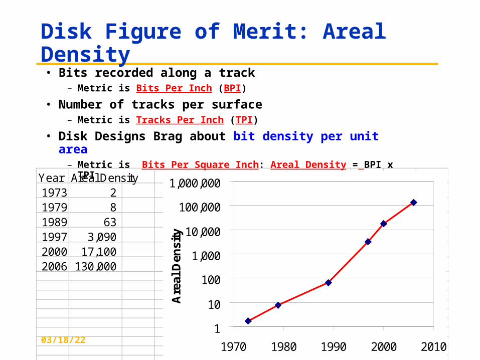
Disk Figure of Merit: Areal Density• Bits recorded along a track
– Metric is Bits Per Inch (BPI)
• Number of tracks per surface– Metric is Tracks Per Inch (TPI)
• Disk Designs Brag about bit density per unit area– Metric is Bits Per Square Inch: Areal Density = BPI x TPI
Year Areal Density1973 2 1979 8 1989 63 1997 3,090 2000 17,100 2006 130,000
1
10
100
1,000
10,000
100,000
1,000,000
1970 1980 1990 2000 2010
Year
Are
al D
ensi
ty
04/19/23 CS252 s06 Storage 6
Historical Perspective
• 1956 IBM Ramac — early 1970s Winchester– Developed for mainframe computers, proprietary interfaces– Steady shrink in form factor: 27 in. to 14 in.
• Form factor and capacity drives market more than performance• 1970s developments
– 5.25 inch floppy disk formfactor (microcode into mainframe)– Emergence of industry standard disk interfaces
• Early 1980s: PCs and first generation workstations• Mid 1980s: Client/server computing
– Centralized storage on file server» accelerates disk downsizing: 8 inch to 5.25
– Mass market disk drives become a reality» industry standards: SCSI, IPI, IDE» 5.25 inch to 3.5 inch drives for PCs, End of proprietary interfaces
• 1900s: Laptops => 2.5 inch drives• 2000s: What new devices leading to new drives?
04/19/23 CS252 s06 Storage 7
Future Disk Size and Performance
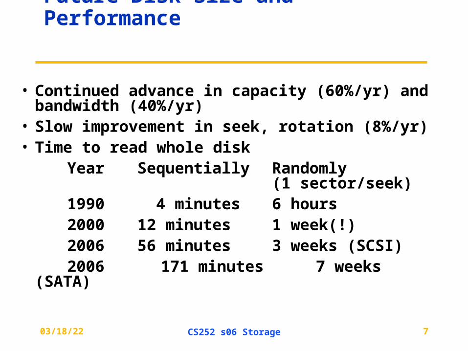
• Continued advance in capacity (60%/yr) and bandwidth (40%/yr)
• Slow improvement in seek, rotation (8%/yr)• Time to read whole disk
Year Sequentially Randomly (1 sector/seek)
1990 4 minutes 6 hours2000 12 minutes 1 week(!)2006 56 minutes 3 weeks (SCSI)2006 171 minutes 7 weeks (SATA)
04/19/23 CS252 s06 Storage 8
Use Arrays of Small Disks?
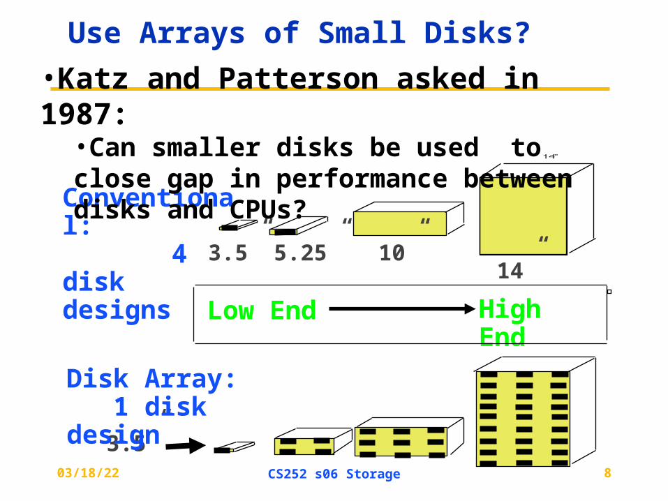
14”10”5.25”3.5”
3.5”
Disk Array: 1 disk design
Conventional: 4 disk designs
Low End High End
•Katz and Patterson asked in 1987: •Can smaller disks be used to close gap in performance between disks and CPUs?
04/19/23 CS252 s06 Storage 9
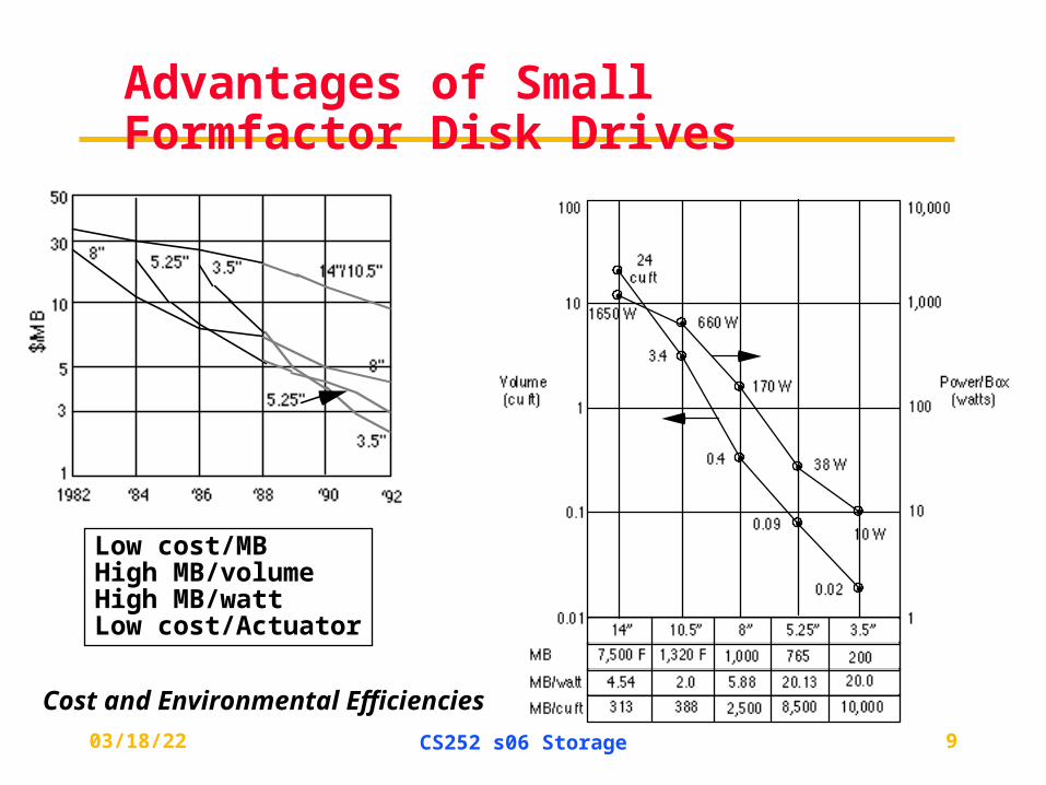
Advantages of Small Formfactor Disk Drives
Low cost/MBHigh MB/volumeHigh MB/wattLow cost/Actuator
Cost and Environmental Efficiencies
04/19/23 CS252 s06 Storage 10
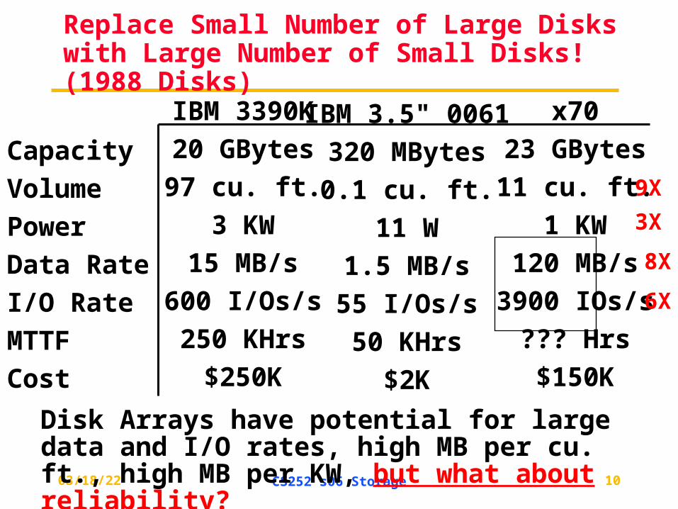
Replace Small Number of Large Disks with Large Number of Small Disks! (1988 Disks)
Capacity
Volume
Power
Data Rate
I/O Rate
MTTF
Cost
IBM 3390K
20 GBytes
97 cu. ft.
3 KW
15 MB/s
600 I/Os/s
250 KHrs
$250K
IBM 3.5" 0061
320 MBytes
0.1 cu. ft.
11 W
1.5 MB/s
55 I/Os/s
50 KHrs
$2K
x70
23 GBytes
11 cu. ft.
1 KW
120 MB/s
3900 IOs/s
??? Hrs
$150K
Disk Arrays have potential for large data and I/O rates, high MB per cu. ft., high MB per KW, but what about reliability?
9X
3X
8X
6X
04/19/23 CS252 s06 Storage 11
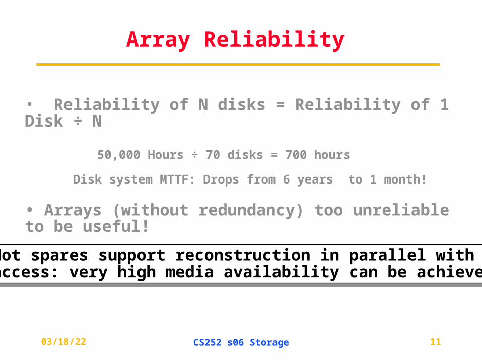
Array Reliability
• Reliability of N disks = Reliability of 1 Disk ÷ N
50,000 Hours ÷ 70 disks = 700 hours
Disk system MTTF: Drops from 6 years to 1 month!
• Arrays (without redundancy) too unreliable to be useful!
Hot spares support reconstruction in parallel with access: very high media availability can be achievedHot spares support reconstruction in parallel with access: very high media availability can be achieved
04/19/23 CS252 s06 Storage 12
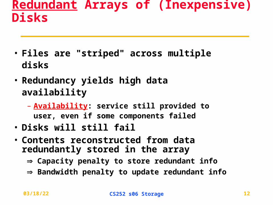
Redundant Arrays of (Inexpensive) Disks
• Files are "striped" across multiple disks
• Redundancy yields high data availability
– Availability: service still provided to user, even if some components failed
• Disks will still fail• Contents reconstructed from data redundantly
stored in the array Capacity penalty to store redundant info
Bandwidth penalty to update redundant info
04/19/23 CS252 s06 Storage 13
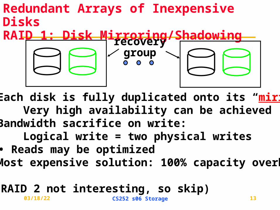
Redundant Arrays of Inexpensive DisksRAID 1: Disk Mirroring/Shadowing
• Each disk is fully duplicated onto its “mirror” Very high availability can be achieved• Bandwidth sacrifice on write: Logical write = two physical writes
• Reads may be optimized• Most expensive solution: 100% capacity overhead
• (RAID 2 not interesting, so skip)
recoverygroup
04/19/23 CS252 s06 Storage 14
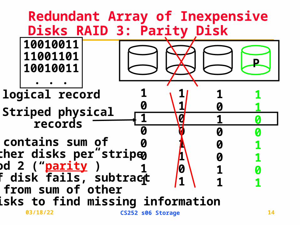
Redundant Array of Inexpensive Disks RAID 3: Parity Disk
P
100100111100110110010011
. . .logical record 1
0100011
11001101
10100011
11001101
P contains sum ofother disks per stripe mod 2 (“parity”)If disk fails, subtract P from sum of other disks to find missing information
Striped physicalrecords
04/19/23 CS252 s06 Storage 15
RAID 3
• Sum computed across recovery group to protect against hard disk failures, stored in P disk
• Logically, a single high capacity, high transfer rate disk: good for large transfers
• Wider arrays reduce capacity costs, but decreases availability
• 33% capacity cost for parity if 3 data disks and 1 parity disk
04/19/23 CS252 s06 Storage 16
Inspiration for RAID 4
• RAID 3 relies on parity disk to discover errors on Read
• But every sector has an error detection field• To catch errors on read, rely on error
detection field vs. the parity disk• Allows independent reads to different disks
simultaneously
04/19/23 CS252 s06 Storage 17
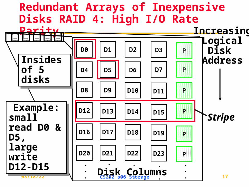
Redundant Arrays of Inexpensive Disks RAID 4: High I/O Rate Parity
D0 D1 D2 D3 P
D4 D5 D6 PD7
D8 D9 PD10 D11
D12 PD13 D14 D15
PD16 D17 D18 D19
D20 D21 D22 D23 P
.
.
.
.
.
.
.
.
.
.
.
.
.
.
.Disk Columns
IncreasingLogicalDisk
Address
Stripe
Insides of 5 disksInsides of 5 disks
Example:small read D0 & D5, large write D12-D15
Example:small read D0 & D5, large write D12-D15
04/19/23 CS252 s06 Storage 18
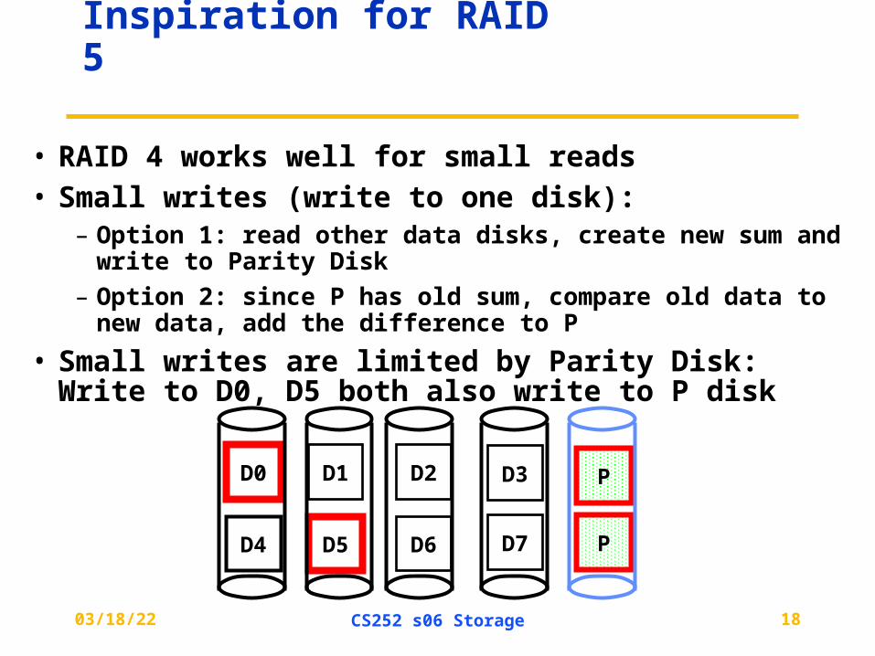
Inspiration for RAID 5
• RAID 4 works well for small reads• Small writes (write to one disk):
– Option 1: read other data disks, create new sum and write to Parity Disk
– Option 2: since P has old sum, compare old data to new data, add the difference to P
• Small writes are limited by Parity Disk: Write to D0, D5 both also write to P disk
D0 D1 D2 D3 P
D4 D5 D6 PD7
04/19/23 CS252 s06 Storage 19
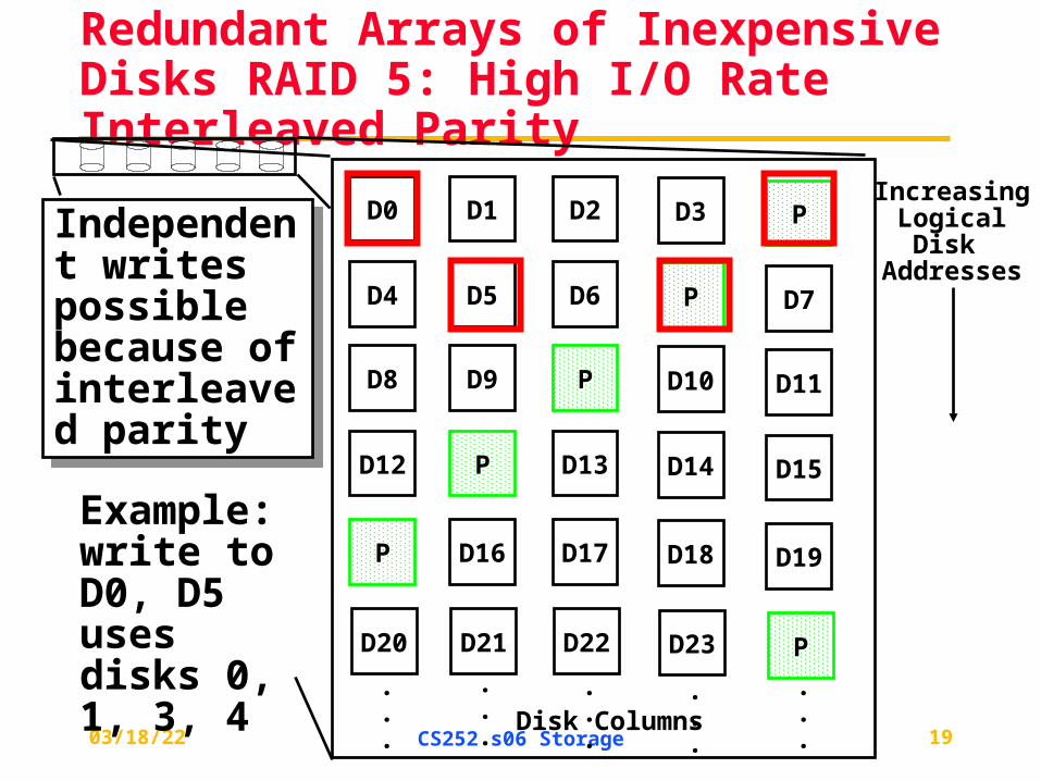
Redundant Arrays of Inexpensive Disks RAID 5: High I/O Rate Interleaved Parity
Independent writespossible because ofinterleaved parity
Independent writespossible because ofinterleaved parity
D0 D1 D2 D3 P
D4 D5 D6 P D7
D8 D9 P D10 D11
D12 P D13 D14 D15
P D16 D17 D18 D19
D20 D21 D22 D23 P
.
.
.
.
.
.
.
.
.
.
.
.
.
.
.Disk Columns
IncreasingLogical
Disk Addresses
Example: write to D0, D5 uses disks 0, 1, 3, 4
04/19/23 CS252 s06 Storage 20
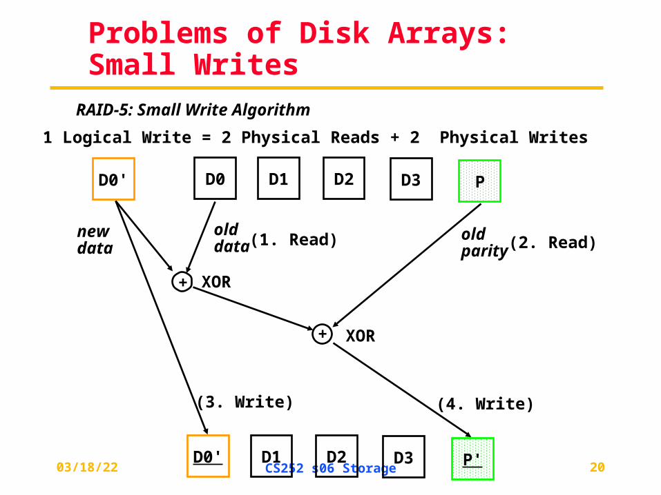
Problems of Disk Arrays: Small Writes
D0 D1 D2 D3 PD0'
+
+
D0' D1 D2 D3 P'
newdata
olddata
old parity
XOR
XOR
(1. Read) (2. Read)
(3. Write) (4. Write)
RAID-5: Small Write Algorithm
1 Logical Write = 2 Physical Reads + 2 Physical Writes

04/19/23 CS252 s06 Storage 21
CS252: Administrivia
• Wed 4/12 – Mon 4/17 Storage (Ch 6)
• RAMP Blue meeting Today 3:30-4 380 Soda
• Makeup Pizza: LaVal’s on Euclid, 6-7 PM
• Project Update Meeting Wednesday 4/19
• Monday 4/24 Quiz 2 5-8 PM (Mainly Ch 4 to 6)
• Wed 4/26 Bad Career Advice / Bad Talk Advice
• Project Presentations Monday 5/1 (all day)
• Project Posters 5/3 Wednesday (11-1 in Soda)
• Final Papers due Friday 5/5 (email Archana, who will post papers on class web site)
04/19/23 CS252 s06 Storage 22
CS252: Administrivia
• Fri 4/14 Read, comment RAID Paper and Homework. Be sure to answer– What was main motivation for RAID in paper?
– Did prediction of processor performance and disk capacity hold?
– How propose balance performance and capacity of RAID 1 to RAID 5? What do you think of it?
– What were some of the open issues? Which were significant
– In retrospect, what do you think were important contributions? What did the authors get wrong?
04/19/23 CS252 s06 Storage 23
RAID 6: Recovering from 2 failures
• Why > 1 failure recovery?– operator accidentally replaces the wrong disk during a
failure
– since disk bandwidth is growing more slowly than disk capacity, the MTT Repair a disk in a RAID system is increasing increases the chances of a 2nd failure during repair since takes longer
– reading much more data during reconstruction meant increasing the chance of an uncorrectable media failure, which would result in data loss
04/19/23 CS252 s06 Storage 24
RAID 6: Recovering from 2 failures• Network Appliance’s row-diagonal parity or RAID-DP
• Like the standard RAID schemes, it uses redundant space based on parity calculation per stripe
• Since it is protecting against a double failure, it adds two check blocks per stripe of data.
– If p+1 disks total, p-1 disks have data; assume p=5
• Row parity disk is just like in RAID 4 – Even parity across the other 4 data blocks in its stripe
• Each block of the diagonal parity disk contains the even parity of the blocks in the same diagonal
04/19/23 CS252 s06 Storage 25
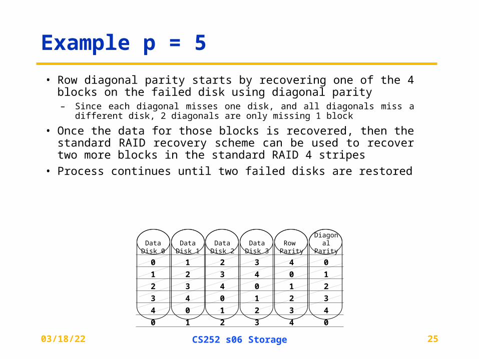
Example p = 5
• Row diagonal parity starts by recovering one of the 4 blocks on the failed disk using diagonal parity
– Since each diagonal misses one disk, and all diagonals miss a different disk, 2 diagonals are only missing 1 block
• Once the data for those blocks is recovered, then the standard RAID recovery scheme can be used to recover two more blocks in the standard RAID 4 stripes
• Process continues until two failed disks are restored
Data Disk 0
Data Disk 1
Data Disk 2
Data Disk 3
Row Parity
Diagonal Parity
0 1 2 3 4 0
1 2 3 4 0 1
2 3 4 0 1 2
3 4 0 1 2 3
4 0 1 2 3 4
0 1 2 3 4 0
04/19/23 CS252 s06 Storage 26
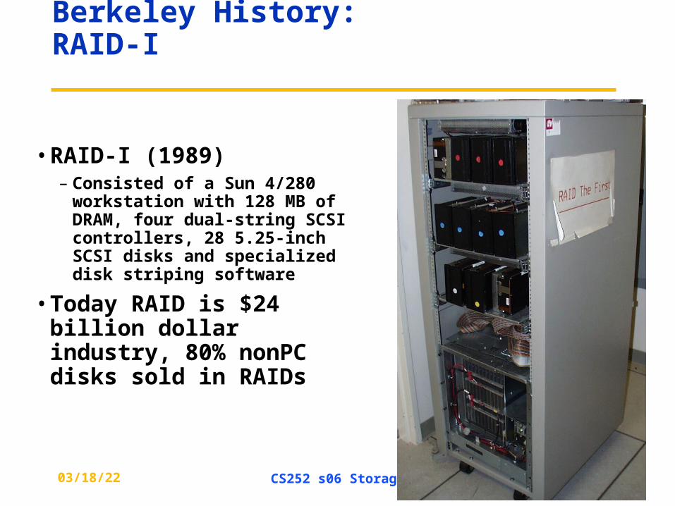
Berkeley History: RAID-I
• RAID-I (1989) – Consisted of a Sun 4/280
workstation with 128 MB of DRAM, four dual-string SCSI controllers, 28 5.25-inch SCSI disks and specialized disk striping software
• Today RAID is $24 billion dollar industry, 80% nonPC disks sold in RAIDs
04/19/23 CS252 s06 Storage 27
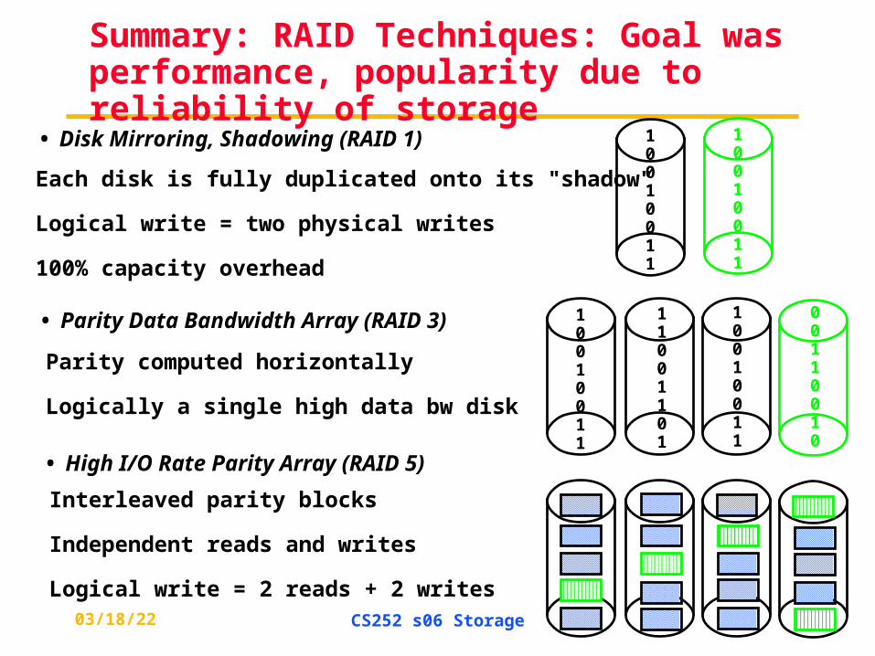
Summary: RAID Techniques: Goal was performance, popularity due to reliability of storage
• Disk Mirroring, Shadowing (RAID 1)
Each disk is fully duplicated onto its "shadow" Logical write = two physical writes
100% capacity overhead
• Parity Data Bandwidth Array (RAID 3)
Parity computed horizontally
Logically a single high data bw disk
• High I/O Rate Parity Array (RAID 5)
Interleaved parity blocks
Independent reads and writes
Logical write = 2 reads + 2 writes
10010011
11001101
10010011
00110010
10010011
10010011
04/19/23 CS252 s06 Storage 28
Definitions
• Examples on why precise definitions so important for reliability
• Is a programming mistake a fault, error, or failure? – Are we talking about the time it was designed
or the time the program is run?
– If the running program doesn’t exercise the mistake, is it still a fault/error/failure?
• If an alpha particle hits a DRAM memory cell, is it a fault/error/failure if it doesn’t change the value?
– Is it a fault/error/failure if the memory doesn’t access the changed bit?
– Did a fault/error/failure still occur if the memory had error correction and delivered the corrected value to the CPU?
04/19/23 CS252 s06 Storage 29
IFIP Standard terminology
• Computer system dependability: quality of delivered service such that reliance can be placed on service
• Service is observed actual behavior as perceived by other system(s) interacting with this system’s users
• Each module has ideal specified behavior, where service specification is agreed description of expected behavior
• A system failure occurs when the actual behavior deviates from the specified behavior
• failure occurred because an error, a defect in module
• The cause of an error is a fault
• When a fault occurs it creates a latent error, which becomes effective when it is activated
• When error actually affects the delivered service, a failure occurs (time from error to failure is error latency)
04/19/23 CS252 s06 Storage 30
Fault v. (Latent) Error v. Failure
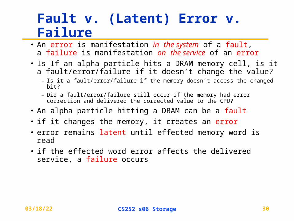
• An error is manifestation in the system of a fault, a failure is manifestation on the service of an error
• Is If an alpha particle hits a DRAM memory cell, is it a fault/error/failure if it doesn’t change the value?
– Is it a fault/error/failure if the memory doesn’t access the changed bit?
– Did a fault/error/failure still occur if the memory had error correction and delivered the corrected value to the CPU?
• An alpha particle hitting a DRAM can be a fault
• if it changes the memory, it creates an error
• error remains latent until effected memory word is read
• if the effected word error affects the delivered service, a failure occurs
04/19/23 CS252 s06 Storage 31
Fault Categories
1. Hardware faults: Devices that fail, such alpha particle hitting a memory cell
2. Design faults: Faults in software (usually) and hardware design (occasionally)
3. Operation faults: Mistakes by operations and maintenance personnel
4. Environmental faults: Fire, flood, earthquake, power failure, and sabotage
• Also by duration:
1. Transient faults exist for limited time and not recurring
2. Intermittent faults cause a system to oscillate between faulty and fault-free operation
3. Permanent faults do not correct themselves over time
04/19/23 CS252 s06 Storage 32
Fault Tolerance vs Disaster Tolerance
• Fault-Tolerance (or more properly, Error-Tolerance): mask local faults(prevent errors from becoming failures)
– RAID disks
– Uninterruptible Power Supplies
– Cluster Failover
• Disaster Tolerance: masks site errors(prevent site errors from causing service failures)
– Protects against fire, flood, sabotage,..
– Redundant system and service at remote site.
– Use design diversity
From Jim Gray’s “Talk at UC Berkeley on Fault Tolerance " 11/9/00
04/19/23 CS252 s06 Storage 33
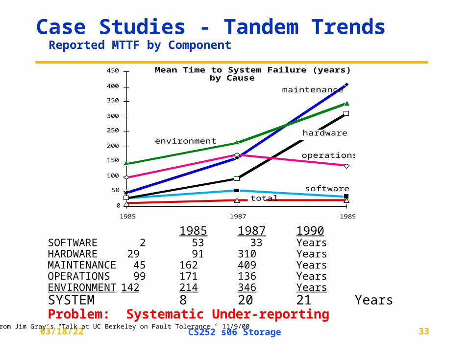
Case Studies - Tandem Trends Reported MTTF by Component
0
50
100
150
200
250
300
350
400
450
1985 1987 1989
software
hardware
maintenance
operations
environment
total
Mean Time to System Failure (years) by Cause
1985 1987 1990SOFTWARE 2 53 33 YearsHARDWARE 29 91 310 YearsMAINTENANCE 45 162 409 YearsOPERATIONS 99 171 136 YearsENVIRONMENT 142 214 346 YearsSYSTEM 8 20 21 YearsProblem: Systematic Under-reporting
From Jim Gray’s “Talk at UC Berkeley on Fault Tolerance " 11/9/00
04/19/23 CS252 s06 Storage 34
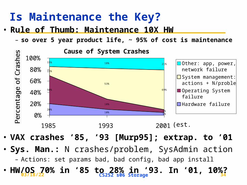
Cause of System Crashes
20%10%
5%
50%
18%
5%
15%
53%
69%
15% 18% 21%
0%
20%
40%
60%
80%
100%
1985 1993 2001
Other: app, power, network failure
System management: actions + N/problem
Operating Systemfailure
Hardware failure
(est.)
• VAX crashes ‘85, ‘93 [Murp95]; extrap. to ‘01
• Sys. Man.: N crashes/problem, SysAdmin action– Actions: set params bad, bad config, bad app install
• HW/OS 70% in ‘85 to 28% in ‘93. In ‘01, 10%?
• Rule of Thumb: Maintenance 10X HW– so over 5 year product life, ~ 95% of cost is maintenance
Is Maintenance the Key?
04/19/23 CS252 s06 Storage 35
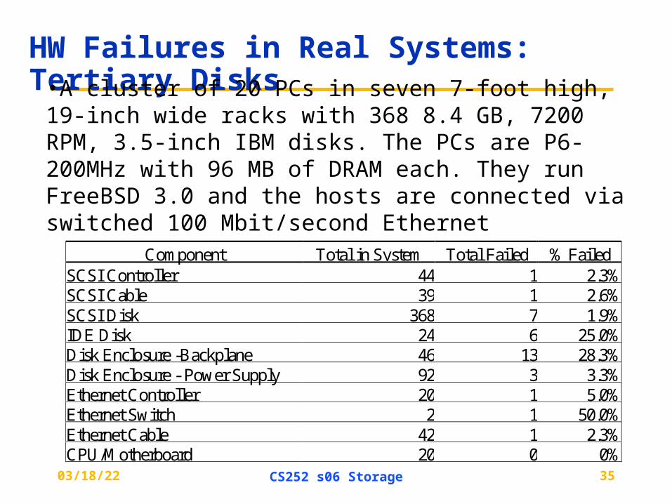
HW Failures in Real Systems: Tertiary Disks
Component Total in System Total Failed % FailedSCSI Controller 44 1 2.3%SCSI Cable 39 1 2.6%SCSI Disk 368 7 1.9%IDE Disk 24 6 25.0%Disk Enclosure -Backplane 46 13 28.3%Disk Enclosure - Power Supply 92 3 3.3%Ethernet Controller 20 1 5.0%Ethernet Switch 2 1 50.0%Ethernet Cable 42 1 2.3%CPU/Motherboard 20 0 0%
•A cluster of 20 PCs in seven 7-foot high, 19-inch wide racks with 368 8.4 GB, 7200 RPM, 3.5-inch IBM disks. The PCs are P6-200MHz with 96 MB of DRAM each. They run FreeBSD 3.0 and the hosts are connected via switched 100 Mbit/second Ethernet
04/19/23 CS252 s06 Storage 36
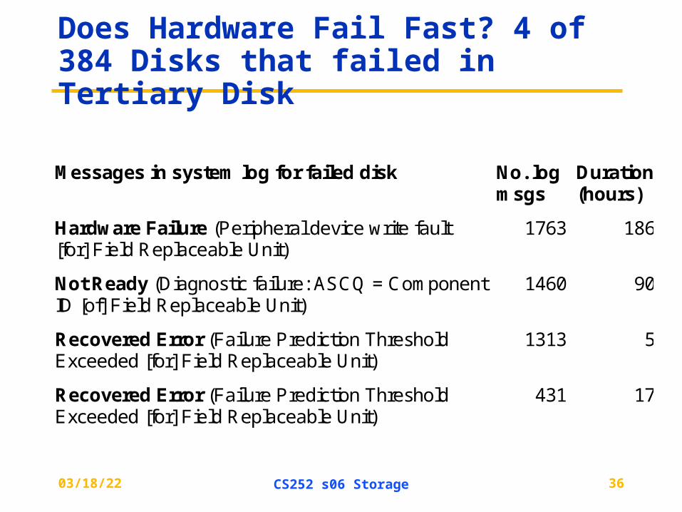
Does Hardware Fail Fast? 4 of 384 Disks that failed in Tertiary Disk
Messages in system log for failed disk No. log msgs
Duration (hours)
Hardware Failure (Peripheral device write fault [for] Field Replaceable Unit)
1763 186
Not Ready (Diagnostic failure: ASCQ = Component ID [of] Field Replaceable Unit)
1460 90
Recovered Error (Failure Prediction Threshold Exceeded [for] Field Replaceable Unit)
1313 5
Recovered Error (Failure Prediction Threshold Exceeded [for] Field Replaceable Unit)
431 17
04/19/23 CS252 s06 Storage 37
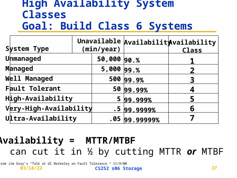
High Availability System ClassesGoal: Build Class 6 Systems
Availability
90.%
99.%
99.9%
99.99%
99.999%
99.9999%
99.99999%
System Type
Unmanaged
Managed
Well Managed
Fault Tolerant
High-Availability
Very-High-Availability
Ultra-Availability
Unavailable(min/year)
50,000
5,000
500
50
5
.5
.05
AvailabilityClass
1234567
UnAvailability = MTTR/MTBFcan cut it in ½ by cutting MTTR or MTBF
From Jim Gray’s “Talk at UC Berkeley on Fault Tolerance " 11/9/00
04/19/23 CS252 s06 Storage 38
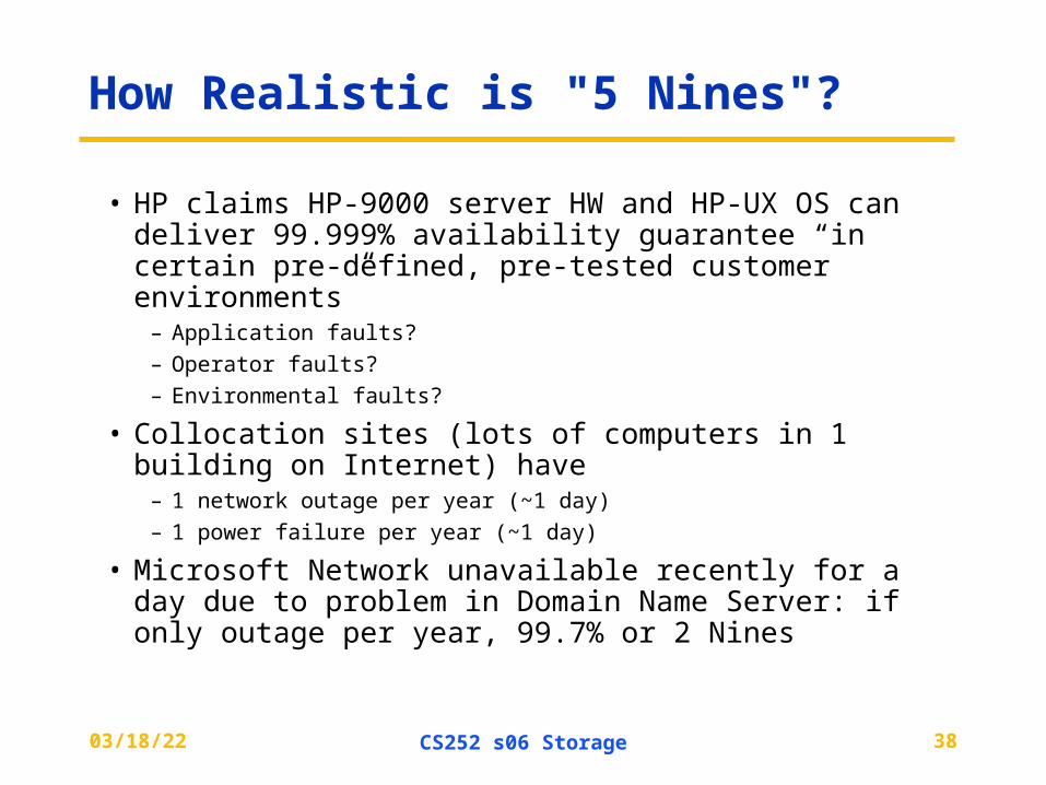
How Realistic is "5 Nines"?
• HP claims HP-9000 server HW and HP-UX OS can deliver 99.999% availability guarantee “in certain pre-defined, pre-tested customer environments”
– Application faults?
– Operator faults?
– Environmental faults?
• Collocation sites (lots of computers in 1 building on Internet) have
– 1 network outage per year (~1 day)
– 1 power failure per year (~1 day)
• Microsoft Network unavailable recently for a day due to problem in Domain Name Server: if only outage per year, 99.7% or 2 Nines
04/19/23 CS252 s06 Storage 39
Outline
• Magnetic Disks
• RAID
• Administrivia
• Advanced Dependability/Reliability/Availability
• I/O Benchmarks, Performance and Dependability
• Intro to Queueing Theory (if we have time)
• Conclusion
04/19/23 CS252 s06 Storage 40
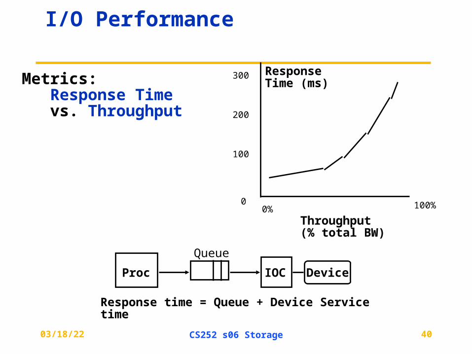
I/O Performance
Response time = Queue + Device Service time
100%
ResponseTime (ms)
Throughput (% total BW)
0
100
200
300
0%
Proc
Queue
IOC Device
Metrics: Response Time vs. Throughput
04/19/23 CS252 s06 Storage 41
I/O Benchmarks
• For better or worse, benchmarks shape a field– Processor benchmarks classically aimed at response time for fixed
sized problem
– I/O benchmarks typically measure throughput, possibly with upper limit on response times (or 90% of response times)
• Transaction Processing (TP) (or On-line TP=OLTP)– If bank computer fails when customer withdraw money, TP system
guarantees account debited if customer gets $ & account unchanged if no $
– Airline reservation systems & banks use TP
• Atomic transactions makes this work
• Classic metric is Transactions Per Second (TPS)
04/19/23 CS252 s06 Storage 42
I/O Benchmarks: Transaction Processing
• Early 1980s great interest in OLTP– Expecting demand for high TPS (e.g., ATM machines, credit cards)– Tandem’s success implied medium range OLTP expands– Each vendor picked own conditions for TPS claims, report only CPU
times with widely different I/O– Conflicting claims led to disbelief of all benchmarks chaos
• 1984 Jim Gray (Tandem) distributed paper to Tandem + 19 in other companies propose standard benchmark
• Published “A measure of transaction processing power,” Datamation, 1985 by Anonymous et. al
– To indicate that this was effort of large group– To avoid delays of legal department of each author’s firm– Still get mail at Tandem to author “Anonymous”
• Led to Transaction Processing Council in 1988– www.tpc.org
04/19/23 CS252 s06 Storage 43
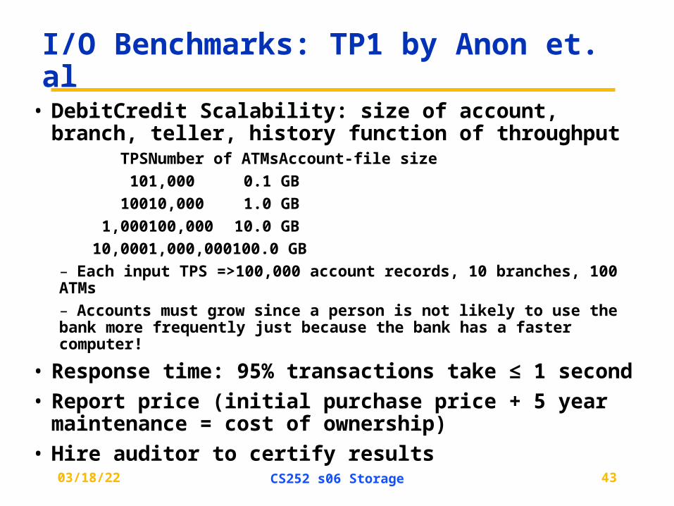
I/O Benchmarks: TP1 by Anon et. al
• DebitCredit Scalability: size of account, branch, teller, history function of throughput TPS Number of ATMs Account-file size
10 1,000 0.1 GB
100 10,000 1.0 GB
1,000 100,000 10.0 GB
10,000 1,000,000 100.0 GB
– Each input TPS =>100,000 account records, 10 branches, 100 ATMs
– Accounts must grow since a person is not likely to use the bank more frequently just because the bank has a faster computer!
• Response time: 95% transactions take ≤ 1 second
• Report price (initial purchase price + 5 year maintenance = cost of ownership)
• Hire auditor to certify results
04/19/23 CS252 s06 Storage 44
Unusual Characteristics of TPC• Price is included in the benchmarks
– cost of HW, SW, and 5-year maintenance agreements included price-performance as well as performance
• The data set generally must scale in size as the throughput increases
– trying to model real systems, demand on system and size of the data stored in it increase together
• The benchmark results are audited– Must be approved by certified TPC auditor, who enforces TPC rules only
fair results are submitted
• Throughput is the performance metric but response times are limited
– eg, TPC-C: 90% transaction response times < 5 seconds
• An independent organization maintains the benchmarks– COO ballots on changes, meetings, to settle disputes...
04/19/23 CS252 s06 Storage 45
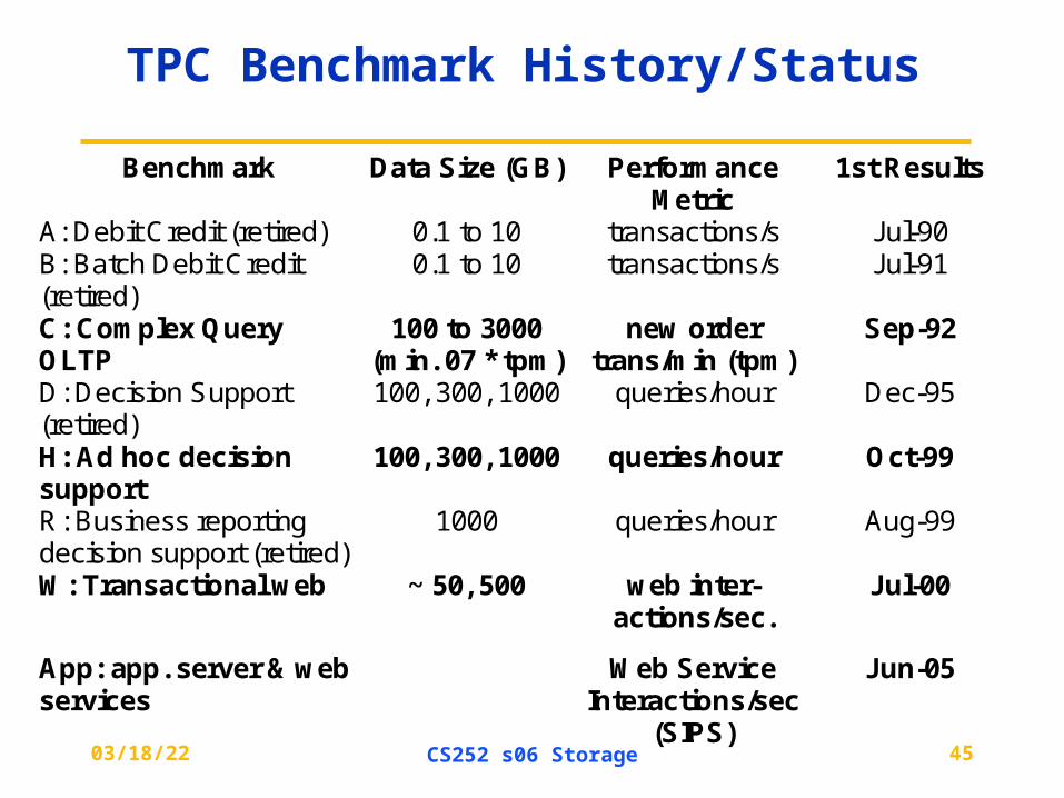
TPC Benchmark History/Status
Benchmark Data Size (GB) Performance Metric
1st Results
A: Debit Credit (retired) 0.1 to 10 transactions/s Jul-90 B: Batch Debit Credit (retired)
0.1 to 10 transactions/s Jul-91
C: Complex Query OLTP
100 to 3000 (min. 07 * tpm)
new order trans/min (tpm)
Sep-92
D: Decision Support (retired)
100, 300, 1000 queries/hour Dec-95
H: Ad hoc decision support
100, 300, 1000 queries/hour Oct-99
R: Business reporting decision support (retired)
1000 queries/hour Aug-99
W: Transactional web ~ 50, 500 web inter-actions/sec.
Jul-00
App: app. server & web services
Web Service Interactions/sec
(SIPS)
Jun-05
04/19/23 CS252 s06 Storage 46
I/O Benchmarks via SPEC
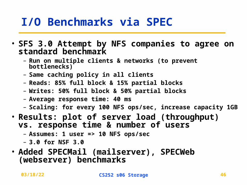
• SFS 3.0 Attempt by NFS companies to agree on standard benchmark
– Run on multiple clients & networks (to prevent bottlenecks)– Same caching policy in all clients– Reads: 85% full block & 15% partial blocks– Writes: 50% full block & 50% partial blocks– Average response time: 40 ms– Scaling: for every 100 NFS ops/sec, increase capacity 1GB
• Results: plot of server load (throughput) vs. response time & number of users
– Assumes: 1 user => 10 NFS ops/sec– 3.0 for NSF 3.0
• Added SPECMail (mailserver), SPECWeb (webserver) benchmarks
04/19/23 CS252 s06 Storage 47
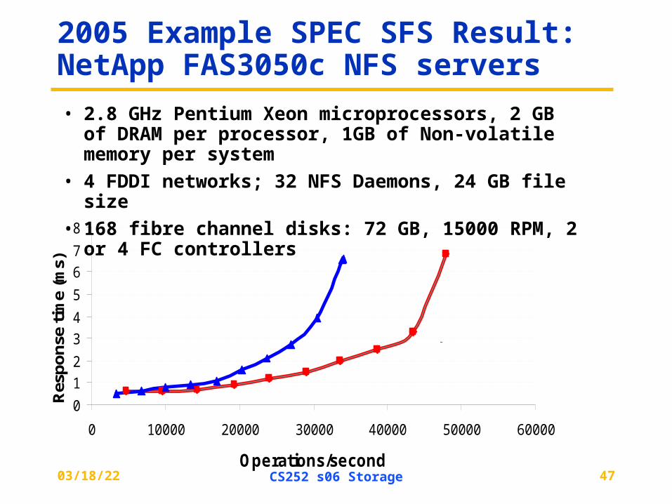
2005 Example SPEC SFS Result: NetApp FAS3050c NFS servers
• 2.8 GHz Pentium Xeon microprocessors, 2 GB of DRAM per processor, 1GB of Non-volatile memory per system
• 4 FDDI networks; 32 NFS Daemons, 24 GB file size
• 168 fibre channel disks: 72 GB, 15000 RPM, 2 or 4 FC controllers
0
1
2
3
4
5
6
7
8
0 10000 20000 30000 40000 50000 60000
Operations/second
Res
pons
e ti
me
(ms) 34,089 47,927
4 processors
2 processors
04/19/23 CS252 s06 Storage 48
Availability benchmark methodology
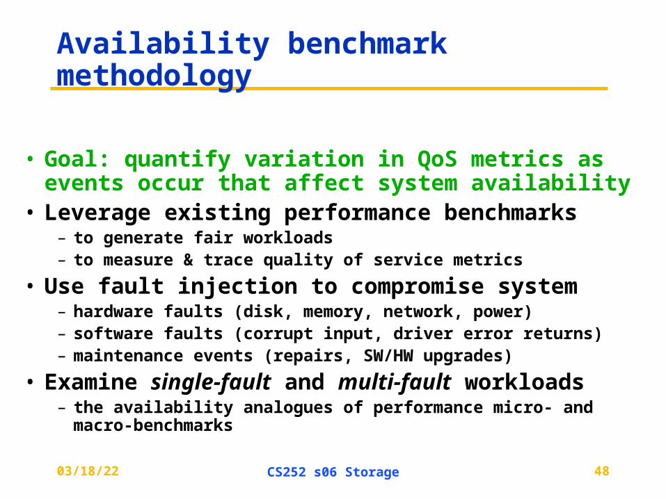
• Goal: quantify variation in QoS metrics as events occur that affect system availability
• Leverage existing performance benchmarks– to generate fair workloads– to measure & trace quality of service metrics
• Use fault injection to compromise system– hardware faults (disk, memory, network, power)– software faults (corrupt input, driver error returns)– maintenance events (repairs, SW/HW upgrades)
• Examine single-fault and multi-fault workloads– the availability analogues of performance micro- and macro-
benchmarks
04/19/23 CS252 s06 Storage 49
Time (minutes)0 10 20 30 40 50 60 70 80 90 100 110
80
100
120
140
160
0
1
2
Hits/sec# failures tolerated
0 10 20 30 40 50 60 70 80 90 100 110
Hit
s p
er s
eco
nd
190
195
200
205
210
215
220
#fai
lure
s t
ole
rate
d
0
1
2
Reconstruction
Reconstruction
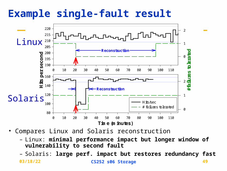
Example single-fault result
• Compares Linux and Solaris reconstruction– Linux: minimal performance impact but longer window of vulnerability
to second fault
– Solaris: large perf. impact but restores redundancy fast
Linux
Solaris
04/19/23 CS252 s06 Storage 50
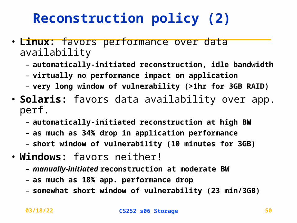
Reconstruction policy (2)
• Linux: favors performance over data availability– automatically-initiated reconstruction, idle bandwidth
– virtually no performance impact on application
– very long window of vulnerability (>1hr for 3GB RAID)
• Solaris: favors data availability over app. perf.– automatically-initiated reconstruction at high BW
– as much as 34% drop in application performance
– short window of vulnerability (10 minutes for 3GB)
• Windows: favors neither!– manually-initiated reconstruction at moderate BW
– as much as 18% app. performance drop
– somewhat short window of vulnerability (23 min/3GB)
04/19/23 CS252 s06 Storage 51
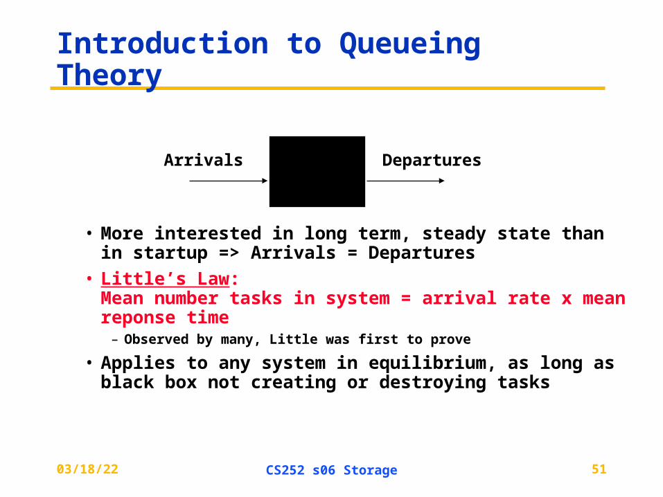
Introduction to Queueing Theory
• More interested in long term, steady state than in startup => Arrivals = Departures
• Little’s Law: Mean number tasks in system = arrival rate x mean reponse time
– Observed by many, Little was first to prove
• Applies to any system in equilibrium, as long as black box not creating or destroying tasks
Arrivals Departures
04/19/23 CS252 s06 Storage 52
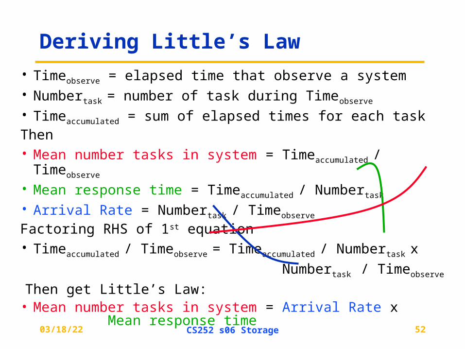
Deriving Little’s Law
• Timeobserve = elapsed time that observe a system• Numbertask = number of task during Timeobserve
• Timeaccumulated = sum of elapsed times for each taskThen• Mean number tasks in system = Timeaccumulated / Timeobserve
• Mean response time = Timeaccumulated / Numbertask
• Arrival Rate = Numbertask / Timeobserve
Factoring RHS of 1st equation• Timeaccumulated / Timeobserve = Timeaccumulated / Numbertask x
Numbertask / Timeobserve
Then get Little’s Law:• Mean number tasks in system = Arrival Rate x
Mean response time
04/19/23 CS252 s06 Storage 53
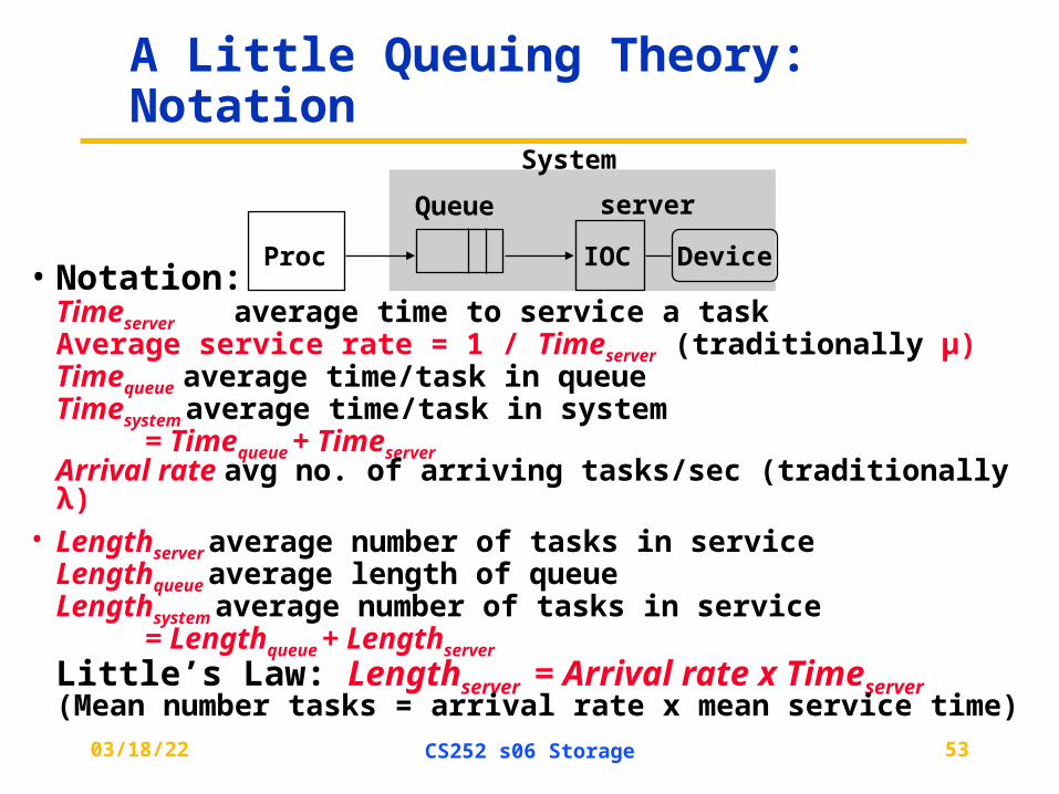
A Little Queuing Theory: Notation
• Notation:Timeserver average time to service a task Average service rate = 1 / Timeserver (traditionally µ) Timequeue average time/task in queue Timesystem average time/task in system
= Timequeue + Timeserver Arrival rate avg no. of arriving tasks/sec (traditionally λ)
• Lengthserver average number of tasks in serviceLengthqueue average length of queue Lengthsystem average number of tasks in service
= Lengthqueue + Lengthserver
Little’s Law: Lengthserver = Arrival rate x Timeserver (Mean number tasks = arrival rate x mean service time)
Proc IOC Device
Queue server
System
04/19/23 CS252 s06 Storage 54
Server Utilization
• For a single server, service rate = 1 / Timeserver
• Server utilization must be between 0 and 1, since system is in equilibrium (arrivals = departures); often called traffic intensity, traditionally ρ)
• Server utilization = mean number tasks in service = Arrival rate x Timeserver
• What is disk utilization if get 50 I/O requests per second for disk and average disk service time is 10 ms (0.01 sec)?
• Server utilization = 50/sec x 0.01 sec = 0.5
• Or server is busy on average 50% of time
04/19/23 CS252 s06 Storage 55
Time in Queue vs. Length of Queue
• We assume First In First Out (FIFO) queue
• Relationship of time in queue (Timequeue) to mean number of tasks in queue (Lengthqueue) ?
• Timequeue = Lengthqueue x Timeserver
+ “Mean time to complete service of task when new task arrives if server is busy”
• New task can arrive at any instant; how predict last part?
• To predict performance, need to know sometime about distribution of events
04/19/23 CS252 s06 Storage 56
Poisson Distribution of Random Variables
• A variable is random if it takes one of a specified set of values with a specified probability
– you cannot know exactly what its next value will be, but you may know the probability of all possible values
• I/O Requests can be modeled by a random variable because OS normally switching between several processes generating independent I/O requests
– Also given probabilistic nature of disks in seek and rotational delays
• Can characterize distribution of values of a random variable with discrete values using a histogram
– Divides range between the min & max values into buckets – Histograms then plot the number in each bucket as columns– Works for discrete values e.g., number of I/O requests?
• What about if not discrete? Very fine buckets
04/19/23 CS252 s06 Storage 57
Characterizing distribution of a random variable
• Need mean time and a measure of variance
• For mean, use weighted arithmetic mean(WAM):
• fi = frequency of task i
• Ti = time for tasks I
weighted arithmetic mean = f1T1 + f2T2 + . . . +fnTn
• For variance, instead of standard deviation, use Variance (square of standard deviation) for WAM:
• Variance = (f1T12 + f2T22 + . . . +fnTn2) – WAM2
– If time is miliseconds, Variance units are square milliseconds!
• Got a unitless measure of variance?
04/19/23 CS252 s06 Storage 58
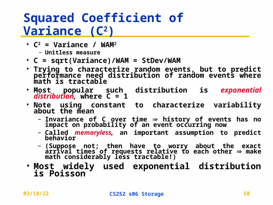
Squared Coefficient of Variance (C2)
• C2 = Variance / WAM2
– Unitless measure• C = sqrt(Variance)/WAM = StDev/WAM• Trying to characterize random events, but to predict
performance need distribution of random events where math is tractable
• Most popular such distribution is exponential distribution, where C = 1
• Note using constant to characterize variability about the mean – Invariance of C over time history of events has no impact on
probability of an event occurring now – Called memoryless, an important assumption to predict behavior – (Suppose not; then have to worry about the exact arrival times of
requests relative to each other make math considerably less tractable!)
• Most widely used exponential distribution is Poisson
04/19/23 CS252 s06 Storage 59
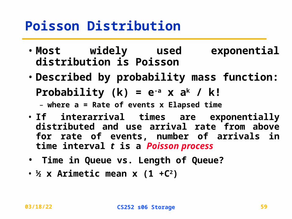
Poisson Distribution
• Most widely used exponential distribution is Poisson
• Described by probability mass function:
Probability (k) = e-a x ak / k! – where a = Rate of events x Elapsed time
• If interarrival times are exponentially distributed and use arrival rate from above for rate of events, number of arrivals in time interval t is a Poisson process
• Time in Queue vs. Length of Queue?
• ½ x Arimetic mean x (1 +C2)
04/19/23 CS252 s06 Storage 60
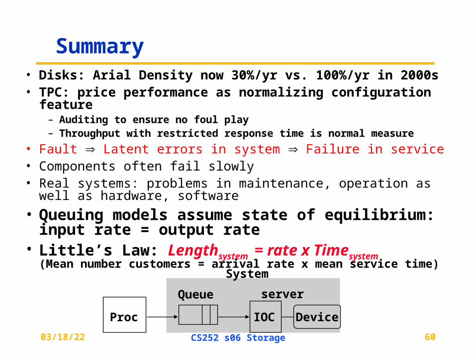
Summary• Disks: Arial Density now 30%/yr vs. 100%/yr in 2000s• TPC: price performance as normalizing configuration feature
– Auditing to ensure no foul play– Throughput with restricted response time is normal measure
• Fault Latent errors in system Failure in service• Components often fail slowly • Real systems: problems in maintenance, operation as well as
hardware, software
• Queuing models assume state of equilibrium: input rate = output rate
• Little’s Law: Lengthsystem = rate x Timesystem (Mean number customers = arrival rate x mean service time)
Proc IOC Device
Queue server
System
Recommended