Download pdf - Efficient PageRank Tracking in Evolving Networks (KDD'15)

Efficient PageRank Tracking

in Evolving Networks

Naoto Ohsaka (UTokyo)

Takanori Maehara (Shizuoka University)

Ken-ichi Kawarabayashi (NII)

KDD’15: Social and Graphs

ERATO Kawarabayashi Large Graph Project

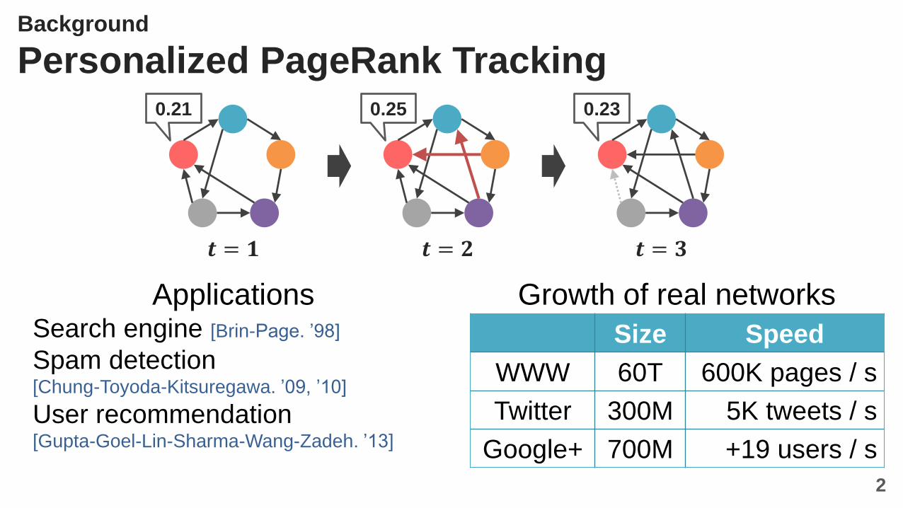
Background

Personalized PageRank Tracking0.21

2

𝒕 = 𝟏 𝒕 = 𝟐 𝒕 = 𝟑

0.25 0.23

ApplicationsSearch engine [Brin-Page. ’98]

Spam detection[Chung-Toyoda-Kitsuregawa. ’09, ’10]

User recommendation[Gupta-Goel-Lin-Sharma-Wang-Zadeh. ’13]

Size Speed

WWW 60T 600K pages / s

Twitter 300M 5K tweets / s

Google+ 700M +19 users / s

Growth of real networks

Background

Existing Work for PageRank Tracking

3

𝒎 random

edge insertions

ScalabilityUpdate time < 0.1s

Error ≈ 10-9

Aggregation/Disaggregation[Chien et al. ’04]

𝒪 𝒎 𝑺 log 1/𝜖 68M edges

Monte-Carlo[Bahmani et al. ’10]

𝒪(𝑚 + log𝑚 /𝝐𝟐) 68M edges

Power methodnaive method

𝒪 𝒎𝟐 log 1/𝜖 11M edges

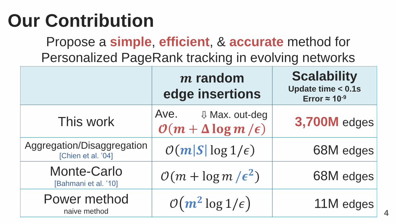
Our Contribution

𝒎 random

edge insertions

ScalabilityUpdate time < 0.1s

Error ≈ 10-9

This workAve.

𝓞 𝒎+ 𝚫 𝐥𝐨𝐠𝒎/𝝐3,700M edges


𝒪 𝒎 𝑺 log 1/𝜖 68M edges


𝒪(𝑚 + log𝑚 /𝝐𝟐) 68M edges

Power methodnaive method

𝒪 𝒎𝟐 log 1/𝜖 11M edges

Propose a simple, efficient, & accurate method for

Personalized PageRank tracking in evolving networks

⇩ Max. out-deg

4

Preliminaries

Definition of Personalized PageRank[Brin-Page. Comput. Networks ISDN Syst.’98] [Jeh-Widom. WWW’03]

Linear equation

A solution 𝑥 of 𝒙 = 𝜶𝑷𝒙 + 𝟏 − 𝜶 𝒃

Random walk modeling web browsing

Moves to a random out-neighbor w.p. 𝛼Jumps to a random vertex w.p. 1 − 𝛼(biased by 𝑏)

Transition matrix

Preference vector

Decay factor = 0.85

Random-walk

interpretation

Stationary

distribution

𝒖

𝒗𝒘

𝒂

5

Preliminaries

Computing PageRank in Static Graphs

Solving eq. 𝑥 = 𝛼𝑃𝑥 + 1 − 𝛼 𝑏

Power method 𝑥(𝜈) = 𝛼𝑃𝑥 𝜈−1 + 1 − 𝛼 𝑏

Gauss-Seidel [Del Corso-Gullí-Romani. Internet Math.’05]

LU/QR factorization [Fujiwara-Nakatsuji-Onizuka-Kitsuregawa. VLDB’12]

Krylov subspace method [Maehara-Akiba-Iwata-Kawarabayashi. VLDB’14]

Estimating the frequency 𝑥𝑣 of visiting 𝑣

Monte-Carlo simulation

6

Preliminaries

Tracking PageRank in Evolving Graphs

Aggregation/disaggregation[Chien-Dwork-Kumar-Simon-Sivakumar. Internet Math.’04]

Apply the power method to a subgraph

Monte-Carlo[Bahmani-Chowdhury. VLDB’10]

Maintain & update random-walk segments

7

Still large

𝛀 𝟏/𝝐𝟐 Too many

𝑮(𝒕)(𝑽, 𝑬(𝒕))

Proposed Method

Problem Setting

8

Given at time 𝑡:Edges inserted to／deleted fromGiven 𝐺 0 , 𝛼, 𝑏 at time 0

Problem at time 0Compute approx.

PPR 𝑥 0 of 𝐺(0)

Problem at time 𝑡Compute approx.

PPR 𝑥 𝑡 of 𝐺(𝑡)

𝒙 𝟎 − 𝒙∗ 𝟎 ∞ < 𝝐

𝑮 𝟎(𝑽, 𝑬(𝟎))

… 𝑮(𝒕 − 𝟏)(𝑽, 𝑬(𝒕 − 𝟏))

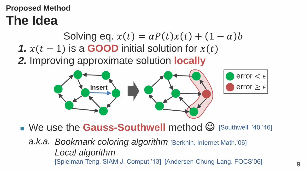
Solving eq. 𝑥 𝑡 = 𝛼𝑃 𝑡 𝑥 𝑡 + 1 − 𝛼 𝑏1. 𝑥(𝑡 − 1) is a GOOD initial solution for 𝑥(𝑡)2. Improving approximate solution locally

Proposed Method

The Idea

9

We use the Gauss-Southwell method

a.k.a. Bookmark coloring algorithm [Berkhin. Internet Math.’06]

Local algorithm[Spielman-Teng. SIAM J. Comput.’13] [Andersen-Chung-Lang. FOCS’06]

[Southwell. ’40,’46]

error < 𝜖

error ≥ 𝜖Insert

𝜈 = 1,2,3, …

𝑖 ←a vertex with largest 𝑟𝑖𝜈−1

If 𝑟𝑖𝜈−1

< 𝜖 terminate

Update 𝑥(𝜈−1) & 𝑟(𝜈−1) locally so that 𝑟𝑖𝜈= 0

𝜈th solution 𝑥 𝜈

𝜈th residual 𝑟(𝜈) = 1 − 𝛼 𝑏 − 𝐼 − 𝛼𝑃 𝑥 𝜈

Goal: 𝑟 𝜈 → 𝟎

Proposed Method

Gauss-Southwell Method [Southwell. ’40,’46]

10

# iterations

Stops within 𝑟 0

1−𝛼 𝜖iter.

✔ 𝑟 𝜈 ≤ 𝑟 𝜈−1 − 1 − 𝛼 𝜖

𝒊

𝒗

𝒖

𝒘

+𝛼𝑟𝑖(𝜈−1)

deg


deg+𝛼

𝑟𝑖(𝜈−1)

deg

Accuracy

𝒙∗ − 𝒙 𝝂∞≤

𝝐

𝟏−𝜶

✔ 𝑟𝑖(𝜈)

< 𝜖

Proposed Method

Overview

11

At time 𝑡:

𝑥 𝑡 (0) = 𝑥 𝑡 − 1

𝑟 𝑡 0 = 𝑟 𝑡 − 1 + 𝛼 𝑃 𝑡 − 𝑃 𝑡 − 1 𝑥 𝑡 − 1

Apply the Gauss-Southwell method

depends on 1

At time 𝑡:

𝑥 𝑡 (0) = 𝑥 𝑡 − 1

𝑟 𝑡 0 = 𝑟 𝑡 − 1 + 𝛼 𝑃 𝑡 − 𝑃 𝑡 − 1 𝑥 𝑡 − 1

Apply the Gauss-Southwell method

Proposed Method

Performance Analysis

12

Increase of 𝒓 𝟏

Computation time of = 𝒪 Δ × #iters.Max. out-deg ⇧

𝒊

𝒗

𝒖

𝒘


deg


deg+𝛼

𝑟𝑖(𝜈−1)

degHow small?

Proposed Method

Performance Analysis: Any Change

13

𝑮(𝒕 − 𝟏) 𝑮(𝒕)

Consider any change including full construction

increase of 𝑟 1 ≤ 𝟐𝜶

Same as static computation

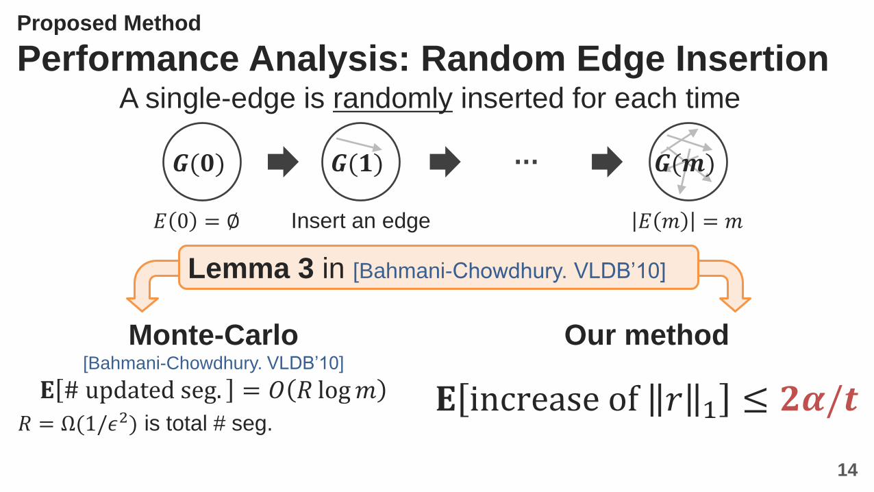
Proposed Method

Performance Analysis: Random Edge Insertion

14

Monte-Carlo[Bahmani-Chowdhury. VLDB’10]

𝐄 # updated seg. = 𝑂 𝑅 log𝑚

𝑅 = Ω(1/𝜖2) is total # seg.

Our method

𝐄 increase of 𝑟 1 ≤ 𝟐𝜶/𝒕

A single-edge is randomly inserted for each time

𝑮(𝟎)

𝐸 0 = ∅ Insert an edge 𝐸 𝑚 = 𝑚

… 𝑮(𝒎)𝑮(𝟏)

Lemma 3 in [Bahmani-Chowdhury. VLDB’10]

Proposed Method

Performance Analysis: Results

15

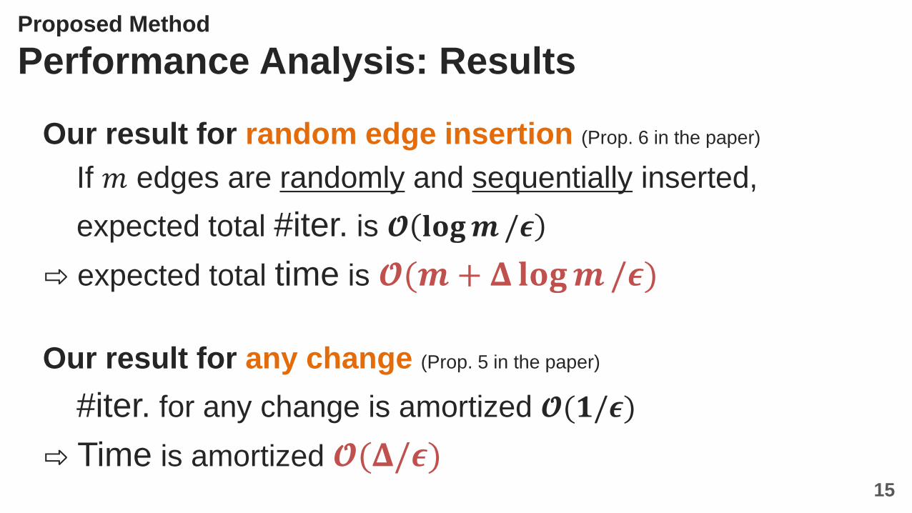
Our result for random edge insertion (Prop. 6 in the paper)

If 𝑚 edges are randomly and sequentially inserted,

expected total #iter. is 𝓞 𝐥𝐨𝐠𝒎/𝝐

⇨ expected total time is 𝓞(𝒎+ 𝚫 𝐥𝐨𝐠𝒎/𝝐)

Our result for any change (Prop. 5 in the paper)

#iter. for any change is amortized 𝓞(𝟏/𝝐)

⇨ Time is amortized 𝓞(𝚫/𝝐)

Experiments

Setting: Single-edge Insertion

Parameter settings

𝛼 = 0.85

𝑏 has 100 non-zero elements

𝜖 = 10−9

16

𝑮(𝟎) 𝑮(𝟏) 𝑮(𝟏𝟎𝟓)

Except the last

100,000 edgesAdd an edge The whole graph

…

chronologicallyor

randomly

Experiments

Efficiency Comparison: Time for an Edge Insertionweb-Google

[SNAP]

𝑉 =1M

𝐸 =5M

Wikipedia[KONECT]

𝑉 = 2M

𝐸 =40M

twitter-2010[LAW]

𝑉 = 142M

𝐸 =1,500M

uk-2007-05[LAW]

𝑉 = 105M

𝐸 =3,700M

This work 7 μs 77 μs 29,383 μs 2 μs


320 μs 40,336 μs >100,000 μs >100,000 μs


444 μs 9,196 μs >100,000 μs >100,000 μs

Warm start power method 80,994 μs >100,000 μs >100,000 μs >100,000 μs

From scratch power method >100,000 μs >100,000 μs >100,000 μs >100,000 μs

17Environment: Intel Xeon E5-2690 2.90GHz CPU with 256GB memory

[KONECT] The Koblenz Network Collection http://konect.uni-koblenz.de/networks/

[LAW] Laboratory for Web Algorithmics http://law.di.unimi.it/datasets.php

[SNAP] Stanford Large Network Dataset Collection http://snap.stanford.edu/data/

http://konect.uni-koblenz.de/networks/

http://law.di.unimi.it/datasets.php

http://snap.stanford.edu/data/

Experiments

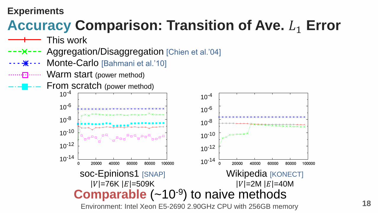
Accuracy Comparison: Transition of Ave. 𝐿1 Error

18

This work

Aggregation/Disaggregation [Chien et al.’04]

Monte-Carlo [Bahmani et al.’10]

Warm start (power method)

From scratch (power method)

Wikipedia [KONECT]

𝑉 =2M 𝐸 =40M

Environment: Intel Xeon E5-2690 2.90GHz CPU with 256GB memory

10-4

10-8

10-10

10-6

10-12

10-14

soc-Epinions1 [SNAP]

𝑉 =76K 𝐸 =509K

10-4

10-8

10-10

10-6

10-12

10-14

Comparable (~10-9) to naive methods

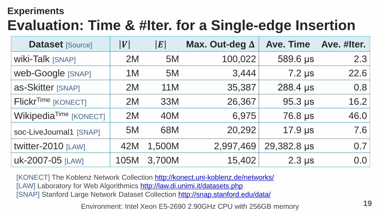
Dataset [Source] 𝑽 𝑬 Max. Out-deg 𝚫 Ave. Time Ave. #Iter.

wiki-Talk [SNAP] 2M 5M 100,022 589.6 μs 2.3

web-Google [SNAP] 1M 5M 3,444 7.2 μs 22.6

as-Skitter [SNAP] 2M 11M 35,387 288.4 μs 0.8

FlickrTime [KONECT] 2M 33M 26,367 95.3 μs 16.2

WikipediaTime [KONECT] 2M 40M 6,975 76.8 μs 46.0

soc-LiveJournal1 [SNAP] 5M 68M 20,292 17.9 μs 7.6

twitter-2010 [LAW] 42M 1,500M 2,997,469 29,382.8 μs 0.7

uk-2007-05 [LAW] 105M 3,700M 15,402 2.3 μs 0.0

Experiments

Evaluation: Time & #Iter. for a Single-edge Insertion




Environment: Intel Xeon E5-2690 2.90GHz CPU with 256GB memory 19




Experiments

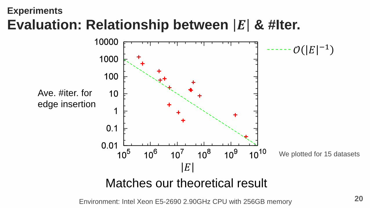
Evaluation: Relationship between 𝑬 & #Iter.

20

𝒪 𝐸 −1

We plotted for 15 datasets

Matches our theoretical result

𝐸

Ave. #iter. for

edge insertion

Environment: Intel Xeon E5-2690 2.90GHz CPU with 256GB memory

Dataset [Source] 𝑽 𝑬 Max. Out-deg 𝚫 Ave. Time Ave. #Iter.

wiki-Talk [SNAP] 2M 5M 100,022 589.6 μs 2.3

web-Google [SNAP] 1M 5M 3,444 7.2 μs 22.6

as-Skitter [SNAP] 2M 11M 35,387 288.4 μs 0.8

FlickrTime [KONECT] 2M 33M 26,367 95.3 μs 16.2

WikipediaTime [KONECT] 2M 40M 6,975 76.8 μs 46.0

soc-LiveJournal1 [SNAP] 5M 68M 20,292 17.9 μs 7.6

twitter-2010 [LAW] 42M 1,500M 2,997,469 29,382.8 μs 0.7

uk-2007-05 [LAW] 105M 3,700M 15,402 2.3 μs 0.0




Experiments

Evaluation: Time & #Iter. for a Single-edge Insertion

What

Happens !?21Environment: Intel Xeon E5-2690 2.90GHz CPU with 256GB memory




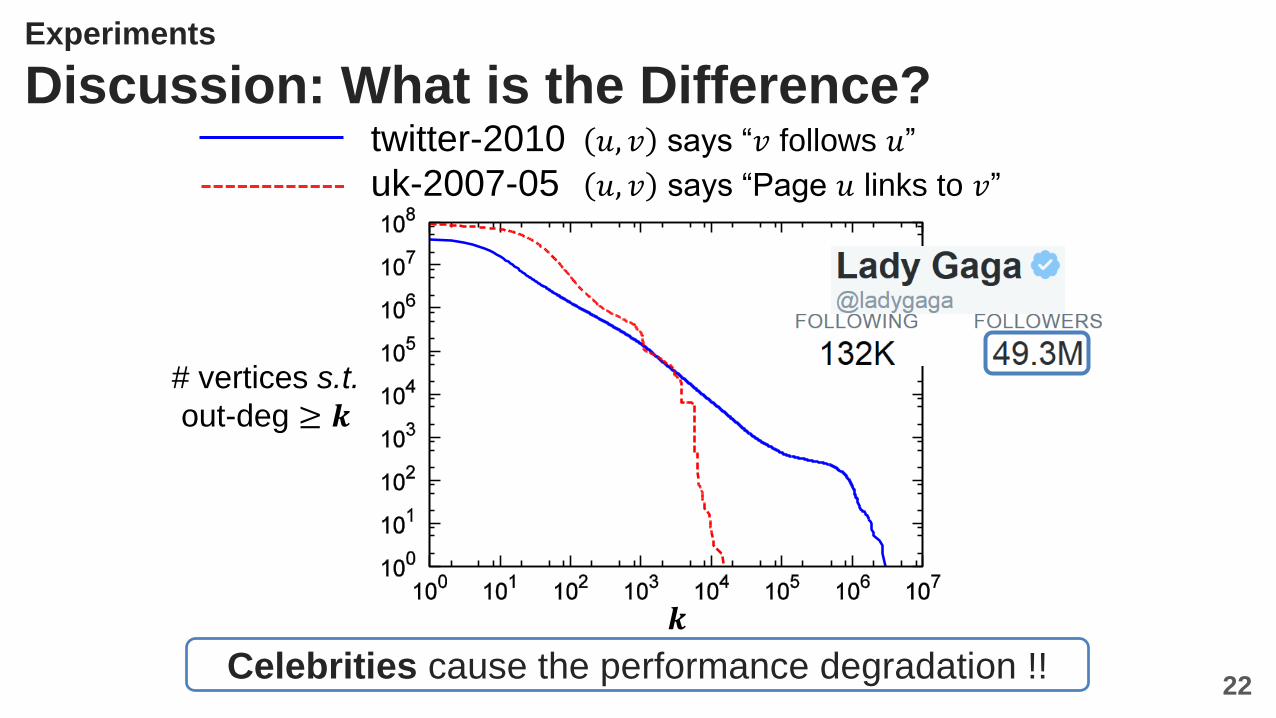
Experiments

Discussion: What is the Difference?twitter-2010 𝑢, 𝑣 says “𝑣 follows 𝑢”

uk-2007-05 𝑢, 𝑣 says “Page 𝑢 links to 𝑣”

𝒌

# vertices s.t.

out-deg ≥ 𝒌

Celebrities cause the performance degradation !!22

Summary

Proposed an efficient & accurate method for

Personalized PageRank tracking in evolving networks

23

Experimentally

Scales to a graph w/ 3.7B edges

Further Speed-up based on our observation

Handle dangling nodes

Theoretically

Ave. 𝓞(𝒎+ 𝚫 𝐥𝐨𝐠𝒎/𝝐)for 𝒎 edge insertions

Future Work