University of Colorado, BoulderCU Scholar
Computer Science Graduate Theses & Dissertations Computer Science
Summer 7-18-2014
Enhancing Recommender Systems Using SocialIndicatorsCharles Michael GartrellUniversity of Colorado Boulder, [email protected]
Follow this and additional works at: http://scholar.colorado.edu/csci_gradetds
Part of the Computer Sciences Commons
This Thesis is brought to you for free and open access by Computer Science at CU Scholar. It has been accepted for inclusion in Computer ScienceGraduate Theses & Dissertations by an authorized administrator of CU Scholar. For more information, please contact [email protected].
Recommended CitationGartrell, Charles Michael, "Enhancing Recommender Systems Using Social Indicators" (2014). Computer Science Graduate Theses &Dissertations. Paper 3.

Enhancing Recommender Systems Using Social Indicators
by
Charles M. Gartrell
B.S., Virginia Tech, 2000
M.S., University of Colorado Boulder, 2008
A thesis submitted to the
Faculty of the Graduate School of the
University of Colorado in partial fulfillment
of the requirements for the degree of
Doctor of Philosophy
Department of Computer Science
2014

This thesis entitled:
Enhancing Recommender Systems Using Social Indicators
written by Charles M. Gartrell
has been approved for the Department of Computer Science
Richard Han
Shivakant Mishra
Qin Lv
John Black
Ulrich Paquet
Date
The final copy of this thesis has been examined by the signatories, and we find that both the content and the
form meet acceptable presentation standards of scholarly work in the above mentioned discipline.
IRB protocol #12-0008
iii
Gartrell, Charles M. (Ph.D., Computer Science)
Enhancing Recommender Systems Using Social Indicators
Thesis directed by Prof. Richard Han
Recommender systems are increasingly driving user experiences on the Internet. In recent years, on-
line social networks have quickly become the fastest growing part of the Web. The rapid growth in social
networks presents a substantial opportunity for recommender systems to leverage social data to improve
recommendation quality, both for recommendations intended for individuals and for groups of users who
consume content together. This thesis shows that incorporating social indicators improves the predictive
performance of group-based and individual-based recommender systems. We analyze the impact of social
indicators through small-scale and large-scale studies, implement and evaluate new recommendation mod-
els that incorporate our insights, and demonstrate the feasibility of using these social indicators and other
contextual data in a deployed mobile application that provides restaurant recommendations to small groups
of users.

Dedication
This thesis is dedicated to all of my family and friends. In particular, I dedicate this thesis to Aurora,
my wife, for her tireless love and encouragement over the years. Without her support this work would not
have been possible.

v
Acknowledgements
Much of the research in this thesis was conducted in collaboration with current and former faculty and
students at the University of Colorado Boulder, including Richard Han, Qin Lv, Shivakant Mishra, Aaron
Beach, Xinyu Xing, Lei Tian, Khaled Alanezi, and a number of current and former staff from Microsoft
Research and R&D, including Ulrich Paquet, Pushmeet Kohli, Ralf Herbrich, John Guiver, John Bronskill,
Yordan Zaykov, Jake Hofman, Tom Minka, Noam Koenigstein, Khaled El-Arini, and Alexandre Passos. My
PhD was primarily funded by the National Science Foundation and the University of Colorado. I thank Nir
Nice at Microsoft R&D Israel for acquiring a license for the Nielsen dataset used in this work.

vi
Contents
Chapter
1 Overview 1
1.1 Thesis Statement . . . . . . . . . . . . . . . . . . . . . . . . . . . . . . . . . . . . . . . . 1
1.2 Research Contributions . . . . . . . . . . . . . . . . . . . . . . . . . . . . . . . . . . . . . 1
2 Introduction 3
2.1 Why are new approaches to social-based recommender systems needed? . . . . . . . . . . . 3
2.2 What is novel about this work? . . . . . . . . . . . . . . . . . . . . . . . . . . . . . . . . . 4
3 Background and Related Work 5
3.1 Social-based Recommender Systems for Individuals . . . . . . . . . . . . . . . . . . . . . . 5
3.2 Recommender Systems for Groups . . . . . . . . . . . . . . . . . . . . . . . . . . . . . . . 7
3.3 Historic TV Viewing Studies . . . . . . . . . . . . . . . . . . . . . . . . . . . . . . . . . . 9
3.4 Context-Aware Systems and Frameworks . . . . . . . . . . . . . . . . . . . . . . . . . . . 9
4 Social-based Recommender Systems for Individuals 11
4.1 Overview . . . . . . . . . . . . . . . . . . . . . . . . . . . . . . . . . . . . . . . . . . . . 11
4.2 Social Links . . . . . . . . . . . . . . . . . . . . . . . . . . . . . . . . . . . . . . . . . . . 12
4.3 Probabilistic Models . . . . . . . . . . . . . . . . . . . . . . . . . . . . . . . . . . . . . . 13
4.3.1 Baseline . . . . . . . . . . . . . . . . . . . . . . . . . . . . . . . . . . . . . . . . . 14
4.3.2 Edge MRF . . . . . . . . . . . . . . . . . . . . . . . . . . . . . . . . . . . . . . . 16
vii
4.3.3 Social Likelihood . . . . . . . . . . . . . . . . . . . . . . . . . . . . . . . . . . . . 18
4.3.4 Average Neighbor . . . . . . . . . . . . . . . . . . . . . . . . . . . . . . . . . . . 20
4.4 Evaluation . . . . . . . . . . . . . . . . . . . . . . . . . . . . . . . . . . . . . . . . . . . . 21
4.4.1 Flixster Data Set . . . . . . . . . . . . . . . . . . . . . . . . . . . . . . . . . . . . 22
4.4.2 Experimental Setup . . . . . . . . . . . . . . . . . . . . . . . . . . . . . . . . . . . 22
4.4.3 Experimental Results . . . . . . . . . . . . . . . . . . . . . . . . . . . . . . . . . . 23
4.5 Summary . . . . . . . . . . . . . . . . . . . . . . . . . . . . . . . . . . . . . . . . . . . . 28
4.6 Appendix . . . . . . . . . . . . . . . . . . . . . . . . . . . . . . . . . . . . . . . . . . . . 28
5 Social-based Recommender Systems for Groups 29
5.1 Overview . . . . . . . . . . . . . . . . . . . . . . . . . . . . . . . . . . . . . . . . . . . . 29
5.2 System Overview . . . . . . . . . . . . . . . . . . . . . . . . . . . . . . . . . . . . . . . . 31
5.2.1 Group Recommender System Architecture . . . . . . . . . . . . . . . . . . . . . . 32
5.2.2 Group Decision Strategies . . . . . . . . . . . . . . . . . . . . . . . . . . . . . . . 33
5.3 System Description . . . . . . . . . . . . . . . . . . . . . . . . . . . . . . . . . . . . . . . 34
5.3.1 Group Descriptors . . . . . . . . . . . . . . . . . . . . . . . . . . . . . . . . . . . 35
5.3.2 A Heuristic Group Consensus Function . . . . . . . . . . . . . . . . . . . . . . . . 39
5.3.3 Rule-Based Group Consensus Framework . . . . . . . . . . . . . . . . . . . . . . . 40
5.4 Evaluation . . . . . . . . . . . . . . . . . . . . . . . . . . . . . . . . . . . . . . . . . . . . 43
5.4.1 Participants and Groups . . . . . . . . . . . . . . . . . . . . . . . . . . . . . . . . 44
5.4.2 Experimental Methodology . . . . . . . . . . . . . . . . . . . . . . . . . . . . . . 44
5.4.3 Evaluation Measures . . . . . . . . . . . . . . . . . . . . . . . . . . . . . . . . . . 46
5.4.4 Experimental Results . . . . . . . . . . . . . . . . . . . . . . . . . . . . . . . . . . 47
5.5 Summary . . . . . . . . . . . . . . . . . . . . . . . . . . . . . . . . . . . . . . . . . . . . 51
6 A Large-scale Study of Group Viewing Preferences 52
6.1 Overview . . . . . . . . . . . . . . . . . . . . . . . . . . . . . . . . . . . . . . . . . . . . 52
6.2 Dataset . . . . . . . . . . . . . . . . . . . . . . . . . . . . . . . . . . . . . . . . . . . . . 53

viii
6.3 Individual Viewing Patterns . . . . . . . . . . . . . . . . . . . . . . . . . . . . . . . . . . . 56
6.4 Group Viewing Patterns . . . . . . . . . . . . . . . . . . . . . . . . . . . . . . . . . . . . . 57
6.4.1 Group Engagement . . . . . . . . . . . . . . . . . . . . . . . . . . . . . . . . . . . 57
6.4.2 Individual vs. Group Viewing . . . . . . . . . . . . . . . . . . . . . . . . . . . . . 58
6.5 Group Recommendations . . . . . . . . . . . . . . . . . . . . . . . . . . . . . . . . . . . . 62
6.5.1 Modeling Individuals . . . . . . . . . . . . . . . . . . . . . . . . . . . . . . . . . . 63
6.5.2 Preference Aggregation . . . . . . . . . . . . . . . . . . . . . . . . . . . . . . . . 64
6.6 Summary . . . . . . . . . . . . . . . . . . . . . . . . . . . . . . . . . . . . . . . . . . . . 67
7 SocialDining: A Mobile Ad-hoc Group Recommendation Application 69
7.1 Use Cases . . . . . . . . . . . . . . . . . . . . . . . . . . . . . . . . . . . . . . . . . . . . 69
7.1.1 A host invites several friends to meet for lunch at an American Restaurant . . . . . . 69
7.1.2 A user receives an invitation to meet several friends for lunch at an American
Restaurant . . . . . . . . . . . . . . . . . . . . . . . . . . . . . . . . . . . . . . . 71
7.1.3 A user provides information on his individual preferences by rating restaurants . . . 74
7.2 Implementation . . . . . . . . . . . . . . . . . . . . . . . . . . . . . . . . . . . . . . . . . 75
7.3 User Study . . . . . . . . . . . . . . . . . . . . . . . . . . . . . . . . . . . . . . . . . . . 76
7.3.1 SocialDining Restaurant Recommendations . . . . . . . . . . . . . . . . . . . . . . 77
7.3.2 Location Impact on Group Decisions . . . . . . . . . . . . . . . . . . . . . . . . . 79
7.4 Summary . . . . . . . . . . . . . . . . . . . . . . . . . . . . . . . . . . . . . . . . . . . . 80
8 Conclusions 81
8.1 Summary . . . . . . . . . . . . . . . . . . . . . . . . . . . . . . . . . . . . . . . . . . . . 81
8.2 Future Work . . . . . . . . . . . . . . . . . . . . . . . . . . . . . . . . . . . . . . . . . . . 83
Bibliography 85

ix
Tables
Table
4.1 General metrics for the Flixster data set . . . . . . . . . . . . . . . . . . . . . . . . . . . . 22
4.2 RMSE for models with different settings of dimensionality K . . . . . . . . . . . . . . . . 24
4.3 RMSE for cold start users for models with different settings of dimensionality K . . . . . . 24
5.1 Average satisfaction . . . . . . . . . . . . . . . . . . . . . . . . . . . . . . . . . . . . . . . 33
5.2 Minimum misery . . . . . . . . . . . . . . . . . . . . . . . . . . . . . . . . . . . . . . . . 33
5.3 Maximum satisfaction . . . . . . . . . . . . . . . . . . . . . . . . . . . . . . . . . . . . . 34
5.4 Strong social ties . . . . . . . . . . . . . . . . . . . . . . . . . . . . . . . . . . . . . . . . 35
5.5 Weak social ties . . . . . . . . . . . . . . . . . . . . . . . . . . . . . . . . . . . . . . . . . 35
5.6 Categorization of social levels based on daily contact frequency. . . . . . . . . . . . . . . . 36
5.7 Expertise dominant . . . . . . . . . . . . . . . . . . . . . . . . . . . . . . . . . . . . . . . 37
5.8 Categorization of expertise levels based on percentage of movies watched. . . . . . . . . . . 37
5.9 Aggregated RMSE (mean and standard deviation) comparison of different group consensus
functions. . . . . . . . . . . . . . . . . . . . . . . . . . . . . . . . . . . . . . . . . . . . . 50
6.1 Ranked list of genres for individuals with varying demographics. . . . . . . . . . . . . . . . 56
6.2 Ranked list of genres for individuals and groups. The top comparison is shown on varying
age composition; the bottom comparison is pivoted on gender. . . . . . . . . . . . . . . . . 62
7.1 Historical data on completed invitations and recommendations . . . . . . . . . . . . . . . . 78
7.2 Location impact on invitations where the group decision matches a recommendation . . . . 79

x
7.3 Location impact on invitations where the group decision does not match a recommendation . 80

xi
Figures
Figure
4.1 Graphical model for baseline model. . . . . . . . . . . . . . . . . . . . . . . . . . . . . . . 14
4.2 Graphical model for Edge MRF model. Biases are omitted in this graphical model for clarity. 18
4.3 Graphical model for Social Likelihood model. Biases are omitted in this graphical model
for clarity. . . . . . . . . . . . . . . . . . . . . . . . . . . . . . . . . . . . . . . . . . . . . 19
4.4 Graphical model for Average Neighbor model. Biases are omitted in this graphical model
for clarity. . . . . . . . . . . . . . . . . . . . . . . . . . . . . . . . . . . . . . . . . . . . . 20
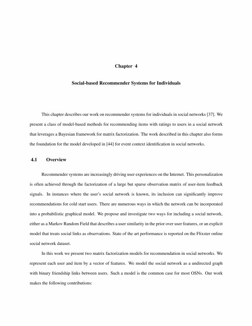
4.5 RMSE for models as a function of the number of samples included in the estimate, after
burn-in. . . . . . . . . . . . . . . . . . . . . . . . . . . . . . . . . . . . . . . . . . . . . . 23
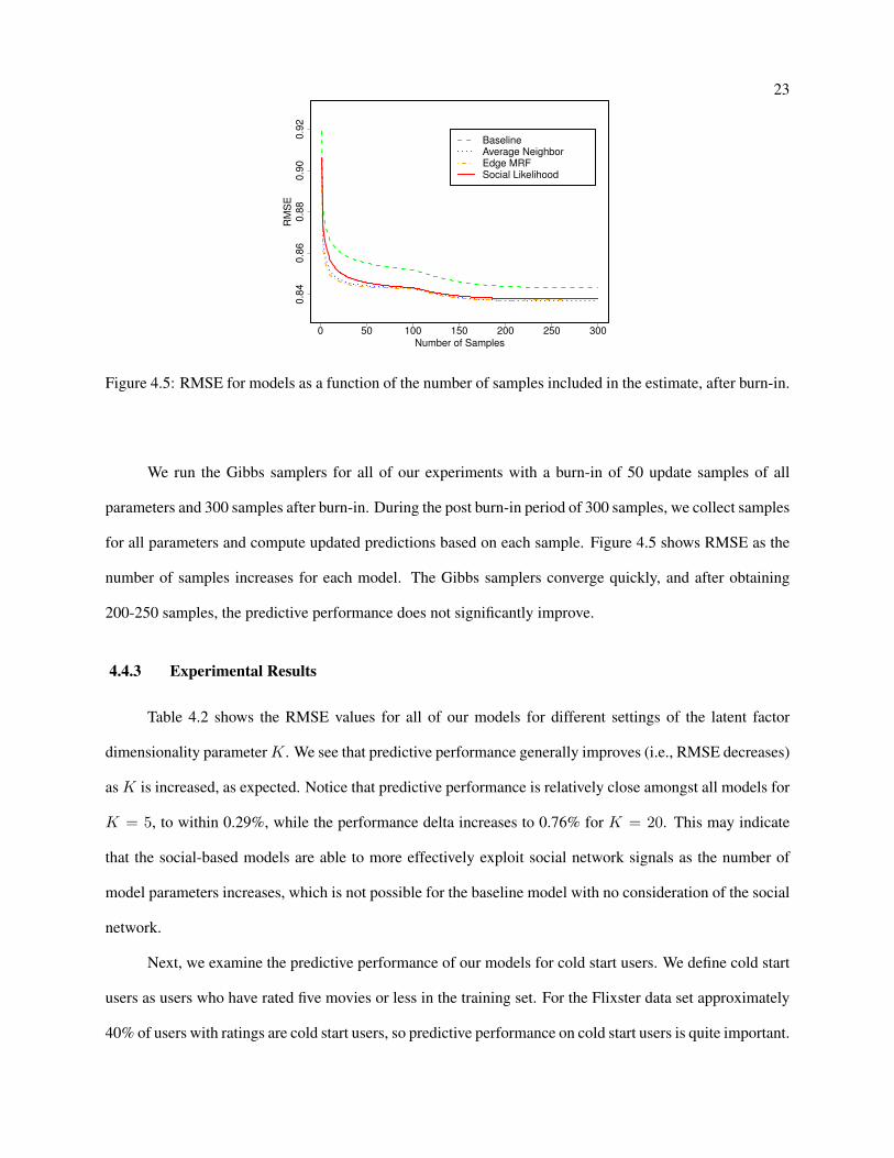
4.6 Performance of models, where users are grouped by the number of observed ratings in the
training data. These results were obtained using K = 5 models. . . . . . . . . . . . . . . . 25
4.7 Performance of baseline models, where users are grouped by the number of observed ratings
in the training data. These results were obtained using K = 5, 10, and 20 models. . . . . . . 25
4.8 Performance of Edge MRF and Average Neighbor models, where users are grouped by the
number of observed ratings in the training data. These results were obtained using K = 5,
10, and 20 models. . . . . . . . . . . . . . . . . . . . . . . . . . . . . . . . . . . . . . . . 25
4.9 Performance of Social Likelihood models, where users are grouped by the number of ob-
served ratings in the training data. These results were obtained using K = 5, 10, and 20
models. . . . . . . . . . . . . . . . . . . . . . . . . . . . . . . . . . . . . . . . . . . . . . 25

xii
4.10 Impact of the value of s on the predictive performance for users with few (0-5), more (40-
80), and many (320-640) ratings. Results were obtaining using the Social Likelihood model
with K = 5. . . . . . . . . . . . . . . . . . . . . . . . . . . . . . . . . . . . . . . . . . . . 26
4.11 Impact of the value of τJ on the predictive performance for users with few (0-5), more (40-
80), and many (320-640) ratings. Results were obtaining using the Average Neighbor model
with K = 5. . . . . . . . . . . . . . . . . . . . . . . . . . . . . . . . . . . . . . . . . . . . 26
4.12 Impact of the number of observed friends per user on the predictive performance for users
with few (0-20), more (60-160), and many (200 or more) friends. In addition to the number
of friends, users are grouped by the number of observed ratings in the training data. Results
were obtaining using the Social Likelihood model with K = 5. . . . . . . . . . . . . . . . . 27
5.1 Group recommender system architecture. . . . . . . . . . . . . . . . . . . . . . . . . . . . 32
5.2 Number of movies watched by individual group members. . . . . . . . . . . . . . . . . . . 38
5.3 Individual ratings vs. group rating in a regular group. . . . . . . . . . . . . . . . . . . . . . 45
5.4 Still frame from 12-person group user study, showing group members discussing their opin-
ions about a movie. . . . . . . . . . . . . . . . . . . . . . . . . . . . . . . . . . . . . . . . 46
5.5 Individual ratings vs. group rating in an expertise-based group. . . . . . . . . . . . . . . . 48
5.6 RMSE comparison of different group consensus functions across 10 different user groups. . 50
6.1 (a) Cumulative distribution of user activity split by individual and group views. (b) Cumula-
tive distribution of telecast popularity by number of viewers. (c) Number of views by group
size. . . . . . . . . . . . . . . . . . . . . . . . . . . . . . . . . . . . . . . . . . . . . . . . 54
6.2 Distribution of views across genres by age and gender. . . . . . . . . . . . . . . . . . . . . 55
6.3 Fraction of views within a group by age and gender. . . . . . . . . . . . . . . . . . . . . . . 57
6.4 Fraction of views within a group by genre. . . . . . . . . . . . . . . . . . . . . . . . . . . . 58
6.5 Similarity between group and individual viewing distributions. . . . . . . . . . . . . . . . . 59
6.6 Distribution of views by genre for adults and children in different group contexts. . . . . . . 60
6.7 Distribution of views by genre for men and women in different group contexts. . . . . . . . 60
xiii
6.8 Modeled and actual probability of group viewing as a function of individual viewing for
2-person, mixed-gender adult couples. . . . . . . . . . . . . . . . . . . . . . . . . . . . . . 65
6.9 (a) mixed gender adult couples with identical preferences, (b) mixed gender adult couples
where one member is indifferent, (c) mixed age pairs where one member is indifferent. . . . 66
7.1 SocialDining main screen. . . . . . . . . . . . . . . . . . . . . . . . . . . . . . . . . . . . 70
7.2 SocialDining invitation creation screen. . . . . . . . . . . . . . . . . . . . . . . . . . . . . 70
7.3 SocialDining invitation time voting screen. . . . . . . . . . . . . . . . . . . . . . . . . . . . 72
7.4 SocialDining invitation restaurant voting screen. . . . . . . . . . . . . . . . . . . . . . . . . 72
7.5 SocialDining restaurant rating screen - search by restaurant name. . . . . . . . . . . . . . . 74
7.6 SocialDining restaurant rating screen - search by restaurant category and promity to user
location. . . . . . . . . . . . . . . . . . . . . . . . . . . . . . . . . . . . . . . . . . . . . . 74
7.7 SocialDining restaurant rating screen showing the list of restaurants currently rated by this
user. . . . . . . . . . . . . . . . . . . . . . . . . . . . . . . . . . . . . . . . . . . . . . . . 75

Chapter 1
Overview
1.1 Thesis Statement
This thesis shows that incorporating social indicators improves the predictive performance of group-based
and individual-based recommender systems. We analyze the impact of social indicators through small-scale
and large-scale studies, implement and evaluate new recommendation models that incorporate our insights,
and demonstrate the feasibility of using these social indicators and other contextual data in a deployed
mobile application that provides restaurant recommendations to small groups of users.
1.2 Research Contributions
(1) Several models for providing recommendations to individuals in social networks are implemented
and evaluated. These models are based on extensions to probabilistic matrix factorization tech-
niques that leverage the social graph to provide improved predictive performance, particularly for
cold-start users.
(2) A new method for providing recommendations to small groups of individuals is proposed and
evaluated. This group recommendation approach utilizes the social and content interests of group
members and uses a novel group consensus framework to model group dynamics.
(3) To demonstrate the feasibility of the above recommendation components, a context-aware mobile
application is implemented, deployed, and evaluated. This application, called SocialDining, pro-
vides recommendations for food and drinking establishments to small, ad-hoc groups of users.

2
(4) We present a large-scale study of television viewing habits, focusing on how individuals adapt
their preferences when consuming content with others in a group setting. Using insight from this
analysis, we propose and evaluate a model for group recommendation based on the demographic
attributes of group members. This work, with a focus on the demographics of group members,
complements the group recommendation approach described above.

Chapter 2
Introduction
This thesis presents, implements, and evaluates new approaches to recommender systems for individ-
uals and groups of individuals that leverage social indicators in novel ways. These approaches are designed
to improve the predictive quality of recommender systems for individuals and small groups. Since online so-
cial networks (OSNs), such as Facebook, have become quite pervasive, this work leverages social networks
as the primary source of social indicators. The recommender systems proposed in this work are evaluated
using small-scale datasets obtained from offline experiments, and large-scale datasets obtained from OSNs
and from household TV viewing data collected by Nielsen. Significant research challenges are involved in
the algorithmic design, implementation, and evaluation of these recommender systems. There are also chal-
lenges involved in the design and implementation of the SocialDining application group recommendation
application, particularly regarding recommendation quality and usability.
2.1 Why are new approaches to social-based recommender systems needed?
Existing approaches to social-based recommender systems for individuals have several limitations.
Briefly, when considering the influence of a user’s friends in the social network, existing approaches do
not consider a notion of user similarity as used in the matrix factorization framework for recommendation,
where ratings predictions are computed as the inner product of latent user factors and item factors that are
learned by the system. We show that such a model of user similarity provides a meaningful improvement
in predictive performance. Additionally, nearly all existing approaches do not consider a fully Bayesian
probabilistic model for social-based recommendation, but instead use an optimization based approach that

4
minimizes a sum-of-squares error function with quadratic regularization terms to find the latent user and
item factors. Such a model requires a search for optimal values of the regularization parameters, which is
computationally quite expensive. The models proposed in this thesis address all of these concerns.
In the case of social-based recommender systems for groups, existing approaches do not fully and
systematically model the influence of social relationships among group members when computing recom-
mendations. Furthermore, existing work does not use large-scale group preference data. We show that an
analysis of large-scale group preference data reveals important insights regarding the differences between
individual and group preference behavior and how group preferences change in various group contexts.
Through systematic analysis and modeling of social relationships and group preference behavior using both
small-scale data gathered from offline experiments and large-scale data gathered from household TV view-
ing, the group-based recommender approaches described in this thesis address all of these issues.
2.2 What is novel about this work?
The work described in this thesis provides some of the first fully probabilistic approaches to mod-
eling the influence of social indicators among individuals for the purposes of recommendation, as well as
some of the first systematic approaches to modeling the impact of social indicators on group preferences.
Novel models for individual and group-based recommendation are developed and evaluated. A detailed
analysis of one of the first available large-scale group preference datasets is presented, revealing differences
between individual and group preferences and providing new insight into how individual preferences are
combined in group settings. Additionally, this work describes the implementation and deployment of one
of the first publicly available mobile applications that leverages social-based approaches to individual and
group recommendation, which is an important milestone.

Chapter 3
Background and Related Work
This chapter reviews prior work related to the topics discussed in this thesis, including social-based
recommendation for individuals, group recommendation, TV viewing studies, and context-aware applica-
tions and frameworks.
3.1 Social-based Recommender Systems for Individuals
The Web has experienced explosive growth over the past decade. Concurrent with the growth of the
Web, recommender systems have attracted increasing attention. Recommender systems aid users in selecting
content that is most relevant to their interests, and notable examples of popular recommender systems are
available for a variety of types of online content, including movies [13], books [1], music [14], and news [7].
Online social networks (OSNs), such as Facebook [2], Google+ [6], and LinkedIn [9], have quickly
become the fastest growing part of the Web. For example, Facebook has grown dramatically over the past
three years, from 100 million users in August 2008 [3] to 1.28 billion users as of April 2014 [4]. This rapid
growth in OSNs presents a substantial opportunity for recommender systems that are able to effectively
leverage OSN data for providing recommendations.
The task of a recommender system is to predict which items will be of interest to a particular user.
Recommender systems are generally implemented using one of two approaches: content filtering and col-
laborative filtering. The content filtering approach builds profiles that describe both users and items. For
example, users may be described by demographic information such as age and gender, and items may be

6
described by attributes such as genre, manufacturer, and author. One popular example of content filtering is
the Music Genome Project [12] used by Pandora [14] to recommend music.
Collaborative filtering is an alternative to content filtering, and relies only on past user behavior
without using explicit user and item profiles. Examples of past user behavior include previous transactions,
such as a user’s purchase history, and users’ ratings on items. Collaborative filtering learns about users and
items based on the items that users have rated and users that have rated similar items. A major appeal of
collaborative filtering systems is that they do not require the creation of user and item profiles, which require
obtaining external information that may not be easy to collect. As such, collaborative filtering systems can
be easily applied to a variety of domains, such as movies, music, etc.
There are two primary approaches to collaborative filtering: neighborhood methods and latent factor
models. Neighborhood methods involve computing relationships between items or between users. Item-
based neighborhood approaches [32, 57, 79] predict a user’s rating for an item based on ratings of similar
items rated by the same user. User-based neighborhood approaches [28, 52] predict a user’s rating for an
item based on the ratings of similar users on the item. Item-based and user-based approaches generally
use a similarity computation algorithm to compute a neighborhood of similar items or users; examples of
similarity algorithms include the Pearson Correlation Coefficient algorithm and the Vector Space Similarity
algorithm.
In contrast to neighborhood methods, latent factor models use an alternative approach that character-
izes users and items in terms of factors inferred from patterns in ratings data. In the case of movies, the
inferred factors might be a measure of traits such as genre aspects (e.g., horror vs. comedy), the extent to
which a movie is appealing to females, etc. For users, each factor indicates the extent to which a user likes
items that have high scores on the corresponding item factors.
Some of the most successful recommender systems that use latent factor models are based on matrix
factorization approaches [73, 77, 78, 84, 86]. As described in Section 4.3, matrix factorization models learn
a mapping of users and items to a join latent feature/factor trait space of dimensionality K. User-item
interactions are modeled as inner products in this trait space. The inner product between each user and item
feature vector captures the user’s overall interest in the item’s traits.

7
Traditionally, most recommender systems have not considered the relationships between users in
social networks. More recently, however, a number of approaches to social-based recommender systems
have been proposed and evaluated. Most OSN-based approaches assume a social network among users and
make recommendations for a user based on the ratings of users that have social connections to the specified
user.
Several neighborhood-based approaches to recommendation in OSNs have been proposed [63, 49, 41,
94]. These approaches generally explore the social network and compute a neighborhood of users trusted
by a specified user. Using this neighbor, these systems provide recommendations by aggregating the ratings
of users in this trust neighborhood. Since these systems require exploration of the social network, these
approaches tend to be slower than social-based latent factor models when computing predictions.
Some latent factor models for social-based recommendation have also been proposed [60, 61, 62,
50, 91]. These methods use matrix factorization to learn latent features for user and items from the ob-
served ratings and from users’ friends (neighbors) in the social network. Experimental results show better
performance than neighborhood-based approaches.
3.2 Recommender Systems for Groups
The problem of group recommendation has been investigated in a number of works [19, 27, 31, 51,
69, 82, 88, 93]. Across this spectrum, various techniques target different types of items (e.g., movies, TV
programs, music) and groups (e.g., family, friends, dynamic social groups).
Most group recommendation techniques consider the preferences of individual users and propose
different strategies to either combine the individual user profiles into a single group (or pseudo user) profile,
and make recommendations for the pseudo user, or generate recommendation lists for individual group
members and merge the lists for group recommendation. Jameson and Smyth’s three main strategies for
merging individual recommendations are average satisfaction, least misery, and maximum satisfaction
[51]; these form the bedrock of group recommendations [19, 31, 64]. In this thesis, the three strategies are
referred to as “preference aggregation functions” or “group decision strategies”. Average satisfaction, which
assumes equal importance across all group members, is used in several group recommendation systems

8
[27, 93, 92]; there is evidence that both average satisfaction and least misery are plausible candidates for
group decisions [64]. Different weights (like weights of family members) have also been used in aggregation
models, rather than an average satisfaction strategy [24]. A more involved consensus function that utilizes
the dissimilarity among group members on top of average satisfaction and least misery strategies, is also
plausible [19]. This consensus function is open to extension, as it does not take other factors that may
affect a group decision into consideration. Social connections and content interests can equally be utilized
in heuristic group consensus functions [38]. The dynamic aspect of group recommendations can also be
overlooked if the group is guaranteed to remain static. For instance, instead of combining the TV preferences
of individual family members, a family-based TV program recommender can base recommendations on the
view history of each household [88]. All of the aforementioned work involves relatively small-scale studies
or prototypes, while other work on group recommendation relied in synthetically generated data from the
MovieLens data set [11, 21, 53, 68]. In contrast, in Chapter 6 we analyze a large-scale dataset consisting of
over a million TV program viewings, of which a quarter are group views.
Smaller practical systems include PolyLens, a group-based movie recommender that targets small,
private, and persistent groups [69]. PolyLens includes facets like the nature of groups, rights of group
members, social value functions, and interfaces for displaying group recommendations. PartyVote provides
a simple democratic mechanism for selecting and playing music at social events, such that each group
member is guaranteed to have at least one of her preferred songs played [82].
Recently, the first available large scale group preference datasets have begun to emerge. The 2011
Challenge on Context-Aware Movie Recommendation (CAMRa 2011), held in conjunction with the ACM
Conference on Recommender Systems, utilized a large scale group preference dataset from the Moviepilot
Web site consisting of over 170,000 users, over 24,000 movies, and nearly 4.4 million ratings [76]. This
dataset also provides information on the household membership for most users. The “group” component
is substantially smaller: there are only 290 households in which the household membership accompanies
a user’s rating, and “group ratings” are lacking. This dataset is not publicly available. A number of group
recommendation approaches have been proposed and evaluated using this dataset, including [25, 40, 43, 48,
67]. Similarly, a large-scale dataset from the BARB organization is used in [81], which consists of about

9
15,000 users, 6,400 households, and 30 million TV program views. However, only 136 of these households
are used in in [81], since the rest lack sufficient group activity. Our work in Chapter 6 differs in that we use
a large dataset with hundreds of thousands of implicit group preferences available in the data in the form
of program views and the time that a user spent watching a program, along with substantial metadata for
individuals, households, and programs.
3.3 Historic TV Viewing Studies
In the early eighties, Webster and Wakshlag [89] analyzed viewing patterns and program-type loy-
alty in group viewing. Their study analyzed how viewing behavior over two categories of programs—
‘situational-comedies’ and ‘crime-action’—differed in individuals and groups. They found that groups that
changed their composition over time exhibited a large variance in their viewing habit. On the other hand,
groups that did not change over time showed more program-type loyalty, and mirrored the viewing trends
of individual users. The analysis did not consider how the composition of the group affected their viewing
patterns. To the best of our knowledge, this question has largely remained unstudied.
Most historic studies of users’ viewing behavior relied on surveys where respondents recorded pro-
gram views in diaries [42, 89]. These studies were based on self-reported data that had a few hundred
respondents. The small size made the results of these studies prone to subject selection biases. As later stud-
ies [65] show, television viewing behavior was affected by demographic characteristics such as age, gender,
income and educational qualifications. Our work in Chapter 6 tries to overcome these problems by using a
large, actively recorded dataset of viewing patterns that comes with detailed demographic information for a
representative sample of viewers.
3.4 Context-Aware Systems and Frameworks
Mark Weiser described the original vision for ubiquitous computing in a world where information pro-
cessing is completely and transparently integrated into everyday activities and objects in [90]. Over the past
two decades, there has been extensive work on context-aware systems and frameworks [20, 45, 26, 66, 34,
80, 33, 87]. Much of this work occurred prior to the advent of online social networks, application-oriented

10
smartphones, and cloud computing. More recent efforts, such as WhozThat [22], integrate Facebook with
mobile phones to provide context-aware music, but do not consider diverse contextual data streams. [75]
surveys recent work regarding the integration of social sensing and pervasive computing services, but does
not consider the broader requirements of context-aware applications, particularly regarding context-aware
recommendation services. In [23], we described our early vision for the SocialFusion framework for context-
aware application and some initial work toward the implementation of that vision. SocialFusion has inspired
the development of the SocialDining application presented in Chapter 7.
Chapter 4
Social-based Recommender Systems for Individuals
This chapter describes our work on recommender systems for individuals in social networks [37]. We
present a class of model-based methods for recommending items with ratings to users in a social network
that leverages a Bayesian framework for matrix factorization. The work described in this chapter also forms
the foundation for the model developed in [44] for event context identification in social networks.
4.1 Overview
Recommender systems are increasingly driving user experiences on the Internet. This personalization
is often achieved through the factorization of a large but sparse observation matrix of user-item feedback
signals. In instances where the user’s social network is known, its inclusion can significantly improve
recommendations for cold start users. There are numerous ways in which the network can be incorporated
into a probabilistic graphical model. We propose and investigate two ways for including a social network,
either as a Markov Random Field that describes a user similarity in the prior over user features, or an explicit
model that treats social links as observations. State of the art performance is reported on the Flixster online
social network dataset.
In this work we present two matrix factorization models for recommendation in social networks. We
represent each user and item by a vector of features. We model the social network as a undirected graph
with binary friendship links between users. Such a model is the common case for most OSNs. Our work
makes the following contributions:

12
• We propose two models that incorporate the social network into a Bayesian framework for matrix
factorization. The first model, called Edge MRF, places the social network in the prior distribution.
The second, called the Social Likelihood model, places the social network in the likelihood func-
tion. To the best of our knowledge, these are some of the first fully Bayesian matrix factorization
models for recommendation in social networks.
• We perform experiments on a large scale, real world dataset obtained from the Flixster.com social
network.
• We report state of the art predictive performance for the Social Likelihood model for cold start
users.
• Based on our experimental results, we conclude that the Social Likelihood model is better for cold
start users than placing the social network in the prior. The Social Likelihood model performs better
in higher dimensions than the social prior alternatives, because the former relies on the same inner
product structure that is used to predict ratings.
The rest of this chapter is organized as follows. We present the probabilistic models and algorithms
for inference in Section 4.3. Section 4.4 presents an evaluation of our models using the Flixster data set.
Finally, Section 4.5 summarizes this work.
4.2 Social Links
For any given social network S with links (i, i′) ∈ S between users i and i′ in a system, we aim to
encode the similarity between the users’ latent feature or taste vectors ui and ui′ ∈ RK in a number of
ways:
(1) For each link, we define an “edge” energy
E(ui,ui′) = −τii′
2‖ui − ui′‖2 , (4.1)

13
which we incorporate into a Markov Random Field (MRF) prior distribution p(U) over all user
features. Furthermore, we may not know the connection strength τii′ , and wish to infer that from
user ratings; in other words, for users with dissimilar tastes we hope that τii′ is negligible.
(2) The links can be treated as explicit observations: define ℓii′ = 1 if (i, i′) ∈ S , and ℓii′ = −1
otherwise. The system can treat ℓii′ as observations with
p(ℓii′ |ui, ui′) = Φ(ℓii′ uTi ui′) , (4.2)
where Φ(z) =∫ x
−∞N (x; 0, 1) dx is the cumulative Normal distribution. This likelihood is akin to
a linear classification model, where an angle of less than 90◦ between ui and ui′ gives likelihood
greater than a half for the discrete value of ℓii′ .
(3) Let S(i) = {i′ : (i, i′) ∈ S} be the set of neighbors for user i. Jamali and Ester [50] use an energy
E(ui,U) = −τJ2
∥
∥
∥
∥
∥
∥
ui −1
|S(i)|∑
i′∈S(i)ui′
∥
∥
∥
∥
∥
∥
2
(4.3)
in the prior, which can also be folded into an MRF. The user feature is a priori expected to lie
inside the convex hull of its neighbors’ feature vectors.
4.3 Probabilistic Models
We observe a user i’s feedback on item j, which we denote by rij ∈ R. Similar to the users, we let
each item have a latent feature vj ∈ RK . Their combination produces the observed rating with noise,
p(rij |ui, vj) = N (rij ; uTi vj , λ
−1) . (4.4)
We furthermore define E(ui) = −αu‖ui‖2/2 and E(vi) = −αv‖vj‖2/2, giving a Normal prior distribu-
tion on V as p(V) =∏
iN (vij ; 0, α−1v I). In the “Social Likelihood” model the prior p(U) would take
the same form. However, in the MRF models we encode S in the prior with either
p(U) ∝ exp
∑
i
E(ui) +∑
(i,i′)∈SE(ui,ui′)
(4.5)

14
Vj Ui
Rij
i#=#1,…,Nj#=#1,…,M
!v !u
"
av0 au0
bv0
a"0 b"0
bu0
bibj
abu0#abv0
!bu!bv
bbv0 bbu0
Figure 4.1: Graphical model for baseline model.
for the “Edge MRF” model or
p(U) ∝ exp
[
∑
i
E(ui) + E(ui,U)
]
(4.6)
for the “Average Neighbor” model. Both of these priors leave any user ui|U\i to be conditionally Gaussian
(read \ as without), and can easily be treated with Gibbs sampling.
We now observe a sparse matrix R with entries rij , and consider the models, and the conditional
distributions of their random variables. The models under consideration are:
4.3.1 Baseline
Rating data in collaborative filtering systems generally exhibit large user and item effects that are
independent of user-item interactions [54] expressed in the baseline model. For example, some users tend to
give higher ratings than others, and some items tend to receive higher ratings than others. We model these
effects with user and item biases, bu and bv, respectively. With these biases, the conditional distribution for
observed ratings becomes
p(rij |ui, vj , bi, bj) = N (rij ; uTi vj + bi + bj , λ
−1) . (4.7)
where bi is the bias for each user and bj is the bias for each item. We place flexible hyperpriors on the
precisions for user and item biases, denoted by αbu and αbv.

15
The baseline model depends on the settings λ, αu, αv, αbu, and αbv, and ignores the social network
and any of the additions to the model that were described in Section 4.2. As the λ and α’s are unknown, we
place a flexible hyperprior – a conjugate Gamma distribution – on each, for example
p(αu) = G(αu ; au0, bu0) =1
Γ(au0)bau0u0 αau0−1e−bu0αu .
Figure 4.1 shows the graphical model for the baseline matrix factorization model.
Inference for all the models will be done through Gibbs sampling [39], which sequentially samples
from the conditional distributions in a graphical model. The samples produced from the arising Markov
chain are from the required posterior distribution if the chain is aperiodic and irreducible.
If we denote the entire set of baseline random variables with θ = {U,V,bu,bv, λ, αu, αv, αbu, αbv},
then samples for ui are drawn from
ui|R, θ\ui∼ N (ui ; µi, Σi)
µi = Σi
λ∑
j∈R(i)
(rij − (bi + bj))vj
Σi =
αuI+ λ∑
j∈R(i)
vjvTj
−1
(4.8)
We’ve defined R(i) as the set of items j rated by user i. A similarly symmetric conditional distribution
holds for each vj .
The conditional distribution bi|R, θbias\bi∼ N (bi ; µi, σ
2i ) is
µi = σ2i
λ∑
j∈R(i)
(rij − (uTi vj + bj))
σ2i =
αbu +∑
j∈R(i)
λ
−1
(4.9)
A similar conditional distribution holds for each bj .

16
Due to the conveniently conjugate prior on αu, its conditional distribution is also a Gamma density,
αu|θ\αu∼ G(αu ; au, bu)
au = au0 +|U|K2
bu = bu0 +1
2
∑
i∈U‖ui‖2 (4.10)
U is defined as the set of all users. A similarly symmetric conditional distribution holds for αv.
The conditional distribution used for sampling αbu is
αbu|θ\αbu∼ G(αbu ; abu, bbu)
abu = abu0 +|U|2
bbu = bbu0 +1
2
∑
i∈Ub2i (4.11)
A similarly symmetric conditional distribution holds for αbv.
Finally, we draw samples for λ from
λ|θ\λ ∼ G(λ ; aλ, bλ)
aλ = aλ0 +|R|2
bλ = bλ0 +1
2
∑
i,j∈R(rij − (uT
i vj + bi + bj))2 (4.12)
We’ve defined R as the set of all ratings.
Algorithm 1 gives a pseudo-algorithm for sampling from θ|R.
The predicted rating rij for any user and item can be determined by averaging Equation (4.4) over
the parameter posterior p(θ|R). If samples θ(t) are simulated from the posterior distribution, this average is
approximated with the Markov chain Monte Carlo (MCMC) estimate
rij =1
T
∑
t
(u(t)Ti v
(t)i + b
(t)i + b
(t)j ) .
4.3.2 Edge MRF
The Edge MRF model uses the prior in (4.5), which additionally depends on the setting of τii′ for all
(i, i′) ∈ S . If the τii′ parameters are flexible, we hope to infer that the similarity connection between two

17
1: initialize U, V, bu, bv, λ, αu, αv, αbu, αbv
2: if edge mrf then
3: initialize τii′ for all (i, i′) ∈ S4: end if
5: // gibbs sampling
6: repeat
7: for items j = 1, . . . , J in random order do
8: sample vj , similar to (4.8)
9: sample bj , similar to (4.9)
10: end for
11: for users i = 1, . . . , I in random order do
12: if baseline then
13: sample ui according to (4.8)
14: sample bi according to (4.9)
15: else if edge mrf then
16: sample τii′ for each i′ ∈ S(i) according to (4.14)
17: sample ui according to (4.13)
18: else if social likelihood then
19: sample hii′ for each i′ ∈ S(i) according to the Appendix
20: sample ui according to (4.16)
21: else
22: // average neighbor
23: sample ui according to (4.17)
24: end if
25: end for
26: sample αu according to (4.10)
27: sample αv similar to (4.10)
28: sample αbu according to (4.11)
29: sample αbv similar to (4.11)
30: sample λ according to (4.12)
31: until sufficient samples have been taken
Algorithm 1: Gibbs sampling
users with vastly different ratings should be negligible, while correlations in very similar users should be
reflected in a higher τii′ connection between them.
We extend the set of random variables to θedge = {θ, τ}. Due to τii′ now appearing in ui’s Markov
blanket in Figure 4.2, the conditional distribution for ui changes to the Gaussian ui|R, θedge\ui∼ N (ui ; µi, Σi)

18
Vj Ui
Rij
i = 1,…,Nj = 1,…,M
Ui'₁
Ui'₂
Ui'f
. . .i' ∈ S(i)
f = |S(i)|
�ii'₁
�ii'₂
�ii'f
�a�0 b�0
�vav0
bv0
�uau0
bu0
Figure 4.2: Graphical model for Edge MRF model. Biases are omitted in this graphical model for clarity.
with
µi = Σi
∑
i′∈S(i)τii′ui′ + λ
∑
j∈R(i)
rijvj
Σi =
αuI+ λ∑
j∈R(i)
vjvTj +
∑
i′∈S(i)τii′I
−1
. (4.13)
There is an interplay in µi above, where ui is a combination of his neighbors ui′ , and items rated vj .
By placing a flexible Gamma prior independently on each τii′ , we can infer each individually with
τii′ |θedge\τii′
∼ G(τii′ ; aτ , bτ )
aτ = aτ0 +1
2
bτ = bτ0 +1
2‖ui − ui′‖2 (4.14)
4.3.3 Social Likelihood
Instead of embedding S in the prior distribution, we can treat it as observations that need to be mod-
eled together with R. To adjust for the fact that there might be an imbalance between the two observations
(for example, |S| might be much larger than the number of observed ratings) we introduce an additional
knob s > 0 in the likelihood. When the graphical model only needs to explain observations ℓii′ = 1, the

19
Vj Ui
Rij
i#=#1,…,Nj#=#1,…,M
Hii' !ii'
s
i'#=#1,…,N
#a#0 b#0
%vav0
bv0
%uau0
bu0
Figure 4.3: Graphical model for Social Likelihood model. Biases are omitted in this graphical model for
clarity.
inclusion of S shouldn’t outweigh any evidence provided by the user ratings. Hence
p(ℓii′ |ui, ui′) = Φ(ℓii′ suTi ui′) . (4.15)
The effect of the likelihood is that ui and ui′ should lie on the same side of a hyperplane perpendicular to
either, like a linear classification model.
We extend the set of random variables to θsl = {θ,H}. H is a set of latent variables that make
sampling from the likelihood possible, and contains an hii′ = suTi uii′ + ǫ with ǫ ∼ N (0, 1). We give its
updates in the Appendix.
Again, the conditional distribution of ui will adapt according to the additions in the graphical model,
shown in Figure 4.3. ui|R,S, θsl\uiis
µi = Σi
s∑
i′∈S(i)hii′ui′ + λ
∑
j∈R(i)
rijvj
Σi =
αuI+ λ∑
j∈R(i)
vjvTj + s
∑
i′∈S(i)ui′u
Ti′
−1
(4.16)
The Social Likelihood model differs from both the Edge MRF and Average Neighbor models through
real-valued latent variables hii′ . If we compare (4.16) to (4.13) and (4.17), we notice that ui is no longer
required to be a positive combination of its neighbors ui′ . Indeed, if ui and ui′ continually give opposite

20
Vj Ui
Rij
i = 1,…,Nj = 1,…,M
Ui'₁
Ui'₂
Ui'f
. . .i' ∈ S(i)
f = |S(i)|�a�0 b�0
�vav0
bv0
�uau0
bu0
�J
Figure 4.4: Graphical model for Average Neighbor model. Biases are omitted in this graphical model for
clarity.
ratings to items, hii′ would be negative. When we compare µi in Equation 4.16 with that of the Edge MRF
model (Equation 4.13), we see that the Social Likelihood model places neighboring users that are similar
to each other in the trait (latent feature) space on the same preference cone/hyperplane in this space, since
the hii′ term in µi is computed using the inner product between a user’s feature vector and his neighbor’s
feature vector. In contrast, the Edge MRF model places neighboring users close to each other based on the
Euclidean distance between their feature vectors, as we see from Equation 4.1. As we will observe from
the experimental results in Section 4.4.3, this distinction between these models has an important impact on
predictive performance.
4.3.4 Average Neighbor
An alternative to specifying a “spring” between the ui’s is to constrain each user’s latent trait to be
an average of those of his friends [50]. The maximum likelihood framework by Jamali and Ester [50] easily
slots into the Gibbs sampler in Algorithm 1 by using the energy function (4.3) in the user prior (4.6). We
add a fixed tunable scale parameter, τJ > 0, to the prior as shown in Figure 4.4, and extend the parameters

21
to θan = {θ, τJ}. The conditional density ui|R,S, θan\uiis
µi = Σi
τJ∑
i′∈S(i)
1
|S(i)|ui′ + λ∑
j∈R(i)
rijvj
Σi =
αuI+ λ∑
j∈R(i)
vjvTj + τJI
−1
(4.17)
We do not sample for τJ because there is no closed-form expression for the conditional density on τJ .
Therefore, because of the difficulty of sampling from this conditional density, we treat τJ as a tunable fixed
parameter.
The Average Neighbor model differs from the Edge MRF model in that each user’s feature vector
is constrained to be the average of the feature vector of his neighbors. This difference is apparent when
comparing the first term of µi in Equation 4.17 and Equation 4.13. By constraining the user’s feature vector
to the average of his neighbors, we allow for less flexibility in learning the user’s feature vector as compared
to the flexible, independent τii′ for each of the user’s social links. In the Average Neighbor model, each of
a user’s neighbors contributes equally to the user’s feature vector, while in the Edge MRF model, the extent
of each neighbor’s contribution varies based on the similarity between the user and neighbor as expressed
by τii′ .
4.4 Evaluation
We evaluated the four models described in Section 4.3 by evaluating their predictive performance on
a publicly available data set obtained from the Flixster.com social networking Web site [5]. In this section
we describe the Flixster data set, our experimental setup, and the results of our performance experiments.

22Metric Flixster
Users 1M
Social Links 5.8M
Ratings 8.2M
Items 49K
Users with Rating 130K
Users with Friend 790K
Table 4.1: General metrics for the Flixster data set
4.4.1 Flixster Data Set
Flixster is an online social network (OSN) that allows users to rate movies, share movie ratings,
discover new movies, and add other users as friends. Each movie rating in Flixster is a discrete value in
the range [0.5, 5] with a step size of 0.5, so there are ten possible rating values (0.5, 1.0, 1.5, . . . ). To our
knowledge, the Flixster data set we use is the largest publicly available OSN data set that contains numeric
ratings for items. We show some general metrics for the Flixster dataset in table 4.1.
4.4.2 Experimental Setup
The metric we use to evaluate predictive performance is root mean square error (RMSE), which is
defined as
RMSE =
√
∑
(i,j)(ri,j − r′i,j)2
n(4.18)
where ri,j is the actual rating for user i and item j from the test set, r′i,j is the predicted rating, and n is the
number of ratings in the test set. We randomly select 80% of the Flixster data as the training set and the
remaining as the test set.
In all of our experiments, we place flexible priors on the α’s and λ in our models by setting au0 =
av0 =√K, bu0 = bv0 = bbu0 = bbv0 = 1, abu0 = abv0 = 2, and aλ0 = bλ0 = 1.5. For the Edge MRF
model, we place a flexible prior on each τii′ by setting aτ0 = bτ0 = 0.15. We set s = 1 for the Social
Likelihood model and τJ = 1 for the Average Neighbor model in all experiments, except where s and τJ
are adjusted between a range of 0.001 and 1000 as stated below.
23
0 50 100 150 200 250 300
0.8
40.8
60.8
80.9
00.9
2
Number of Samples
RM
SE
BaselineAverage NeighborEdge MRFSocial Likelihood
Figure 4.5: RMSE for models as a function of the number of samples included in the estimate, after burn-in.
We run the Gibbs samplers for all of our experiments with a burn-in of 50 update samples of all
parameters and 300 samples after burn-in. During the post burn-in period of 300 samples, we collect samples
for all parameters and compute updated predictions based on each sample. Figure 4.5 shows RMSE as the
number of samples increases for each model. The Gibbs samplers converge quickly, and after obtaining
200-250 samples, the predictive performance does not significantly improve.
4.4.3 Experimental Results
Table 4.2 shows the RMSE values for all of our models for different settings of the latent factor
dimensionality parameter K. We see that predictive performance generally improves (i.e., RMSE decreases)
as K is increased, as expected. Notice that predictive performance is relatively close amongst all models for
K = 5, to within 0.29%, while the performance delta increases to 0.76% for K = 20. This may indicate
that the social-based models are able to more effectively exploit social network signals as the number of
model parameters increases, which is not possible for the baseline model with no consideration of the social
network.
Next, we examine the predictive performance of our models for cold start users. We define cold start
users as users who have rated five movies or less in the training set. For the Flixster data set approximately
40% of users with ratings are cold start users, so predictive performance on cold start users is quite important.

24Model K = 5 K = 10 K = 20
Baseline 0.8590 0.8468 0.8433
Edge MRF 0.8593 0.8458 0.8381
Average Neighbor 0.8581 0.8423 0.8369
Social Likelihood 0.8568 0.8442 0.8380
Table 4.2: RMSE for models with different settings of dimensionality K
Table 4.3 shows the RMSE values for our models for cold start users. Notice that for the baseline
model, predictive performance worsens as K is increased. In contrast, the other models provide approxi-
mately the same or improved predictive performance as model complexity grows. Based on these results,
we see that for cold start users, the Social Likelihood model provides the best predictive performance of the
models that we considered, and that all of the social models outperform the baseline model. Furthermore,
compared to the baseline model, we conclude that the Edge MRF and Average Neighbor models place a
more effective prior distribution on the model parameters by considering the social network. However,
these models are outperformed by the Social Likelihood model, which is able to effectively model the social
network as observations using the inner product similarity between neighbors. Figures 4.7, 4.8, and 4.9
reveal that the performance differences between models tend to be minimized as the number of observed
ratings per user increases.
Figure 4.6 shows that the Social Likelihood model outperforms the other models for users with few
ratings (10 or less ratings). As the number of ratings increases, the predictive performance of all models
converges. Based on the results presented in Table 4.3 and Figure 4.6, we conclude that for cold start users,
the Social Likelihood model is able to leverage the social network more effectively than the other models we
Model K = 5 K = 10 K = 20
Baseline 1.1205 1.14407 1.2180
Edge MRF 1.1424 1.0970 1.0984
Average Neighbor 1.0814 1.0721 1.0662
Social Likelihood 1.0569 1.0583 1.0563
Table 4.3: RMSE for cold start users for models with different settings of dimensionality K
25
●
●
●
● ●
●
●
●
●
0.8
50.9
00.9
51.0
01.0
51.1
01.1
5
Number of Observed Ratings
RM
SE
●
●
●
●
●
●
●
●
●
●
●
●
●●
●
●
●
●
●
●
●
●
● ●
●
●
●
0−5 6−10 −20 −40 −80 −160 −320 −640 >641
BaselineAverage NeighborEdge MRFSocial Likelihood
Figure 4.6: Performance of models, where users are
grouped by the number of observed ratings in the
training data. These results were obtained using
K = 5 models.
●
●
●
● ●●
●
●
●
0.8
0.9
1.0
1.1
1.2
Number of Observed Ratings
RM
SE
●
●
●
●●
●
●
●
●
●
●
●
●
●
●
●
●
●
0−5 6−10 −20 −40 −80 −160 −320 −640 >641
Baseline K = 5Baseline K = 10Baseline K = 20
Figure 4.7: Performance of baseline models, where
users are grouped by the number of observed ratings
in the training data. These results were obtained us-
ing K = 5, 10, and 20 models.
●
●
●
●
●
●
●
●
●
0.8
00.8
50.9
00.9
51.0
01.0
51.1
01.1
5
Number of Observed Ratings
RM
SE
●
●
●
●●
●
●
●
●
●
●
●
●
●
●
●
●
●
●
●
●
●●
●
●
●
●
●
●
●
●●
●
●
●
●
●
●
●
●●
●
●
●
●
0−5 6−10 −20 −40 −80 −160 −320 −640 >641
Average Neighbor K = 5Average Neighbor K = 10Average Neighbor K = 20Edge MRF K = 5Edge MRF K = 10Edge MRF K = 20
Figure 4.8: Performance of Edge MRF and Aver-
age Neighbor models, where users are grouped by
the number of observed ratings in the training data.
These results were obtained using K = 5, 10, and 20
models.
●
●
●
●
● ●
●
●
●
0.8
00.8
50.9
00.9
51.0
01.0
5
Number of Observed Ratings
RM
SE
●
●
●
●●
●
●
●
●
●
●
●
●
●
●
●
●
●
0−5 6−10 −20 −40 −80 −160 −320 −640 >641
Social Likelihood K = 5Social Likelihood K = 10Social Likelihood K = 20
Figure 4.9: Performance of Social Likelihood mod-
els, where users are grouped by the number of ob-
served ratings in the training data. These results were
obtained using K = 5, 10, and 20 models.
26
considered. For users with more ratings, the social network appears to have little to no impact on predictive
performance.
Recall that the s parameter controls the influence of the social network in the Social Likelihood model.
Larger values of s cause the social network to have more influence on the learned latent feature vectors for
users, while smaller values of s cause the social network to have less impact. Figure 4.10 compares the
predictive performance of the Social Likelihood model for different values of s for users with few (0-
5), more (40-80), and many ratings (320-640). These results show that s has little impact on predictive
performance for users with more ratings. However, for cold start users with 0-5 ratings, s has a significant
impact on predictive performance. For these users, the optimal value of s appears to be approximately 1.
These findings regarding the impact of s on cold start users vs. users with more ratings are in agreement
with our other results. Therefore, we conclude that the social network has a significant impact on predictive
performance only for cold start users.
In the Average Neighbor model, the τJ parameter controls the influence of the social network. Fig-
ure 4.11 compares the predictive performance of the Average Neighbor model for different values of τJ for
users with few (0-5), more (40-80), and many ratings (320-640). These results show that τJ has little impact
●
●
●●
●
●
●
0.8
50.9
00.9
51.0
01.0
51.1
0
Value of s parameter
RM
SE
●●
●
● ●
●●
●
● ● ● ● ● ●
0.001 0.01 0.1 1 10 100 1000
Few RatingsMore RatingsMany Ratings
Figure 4.10: Impact of the value of s on the pre-
dictive performance for users with few (0-5), more
(40-80), and many (320-640) ratings. Results were
obtaining using the Social Likelihood model with
K = 5.
●
●
●
● ●
●
●
0.9
1.0
1.1
1.2
Value of τJ parameter
RM
SE
●
●●
●● ●
●
● ● ● ● ● ● ●
0.001 0.01 0.1 1 10 100 1000
Few RatingsMore RatingsMany Ratings
Figure 4.11: Impact of the value of τJ on the pre-
dictive performance for users with few (0-5), more
(40-80), and many (320-640) ratings. Results were
obtaining using the Average Neighbor model with
K = 5.
27
on predictive performance for users with more ratings. However, for cold start users with 0-5 ratings, τJ
has a significant impact on predictive performance. For these users, the optimal value of τJ appears to be
approximately 1. These results are similar to the findings for the impact of the s parameter in the Social
Likelihood model, and provide further evidence that the social network has a significant impact on predictive
performance only for cold start users.
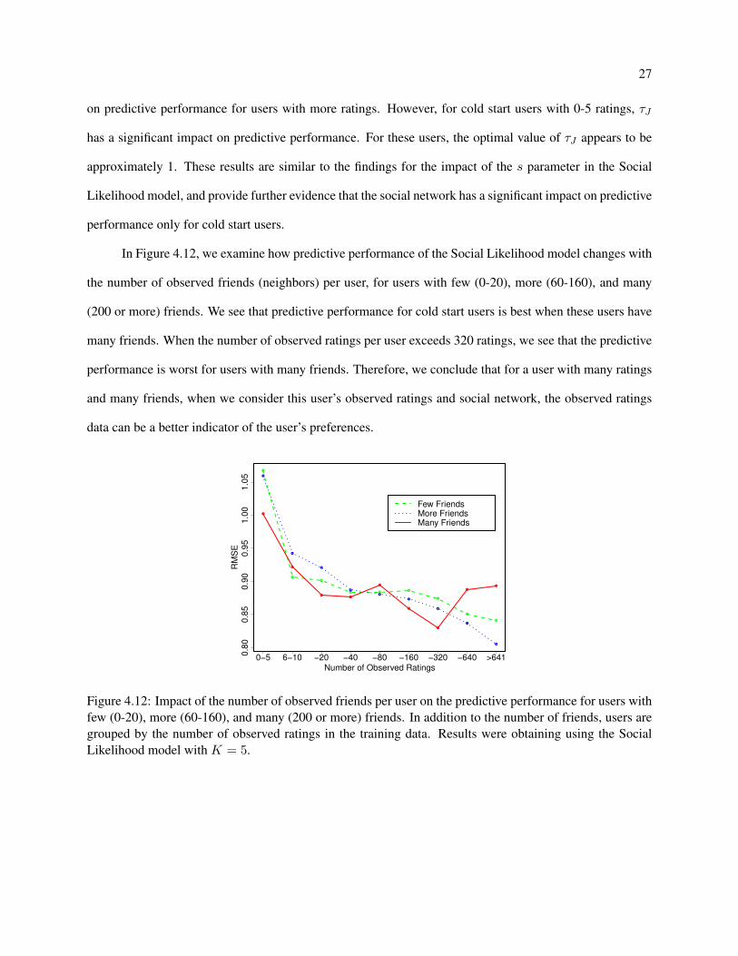
In Figure 4.12, we examine how predictive performance of the Social Likelihood model changes with
the number of observed friends (neighbors) per user, for users with few (0-20), more (60-160), and many
(200 or more) friends. We see that predictive performance for cold start users is best when these users have
many friends. When the number of observed ratings per user exceeds 320 ratings, we see that the predictive
performance is worst for users with many friends. Therefore, we conclude that for a user with many ratings
and many friends, when we consider this user’s observed ratings and social network, the observed ratings
data can be a better indicator of the user’s preferences.
●
●
●
● ●●
●
●
●
0.8
00.8
50.9
00.9
51.0
01.0
5
Number of Observed Ratings
RM
SE
●
●
●
●
●
●
●
●
●
●
●
●●
●
●
●
●
●
0−5 6−10 −20 −40 −80 −160 −320 −640 >641
Few FriendsMore FriendsMany Friends
Figure 4.12: Impact of the number of observed friends per user on the predictive performance for users with
few (0-20), more (60-160), and many (200 or more) friends. In addition to the number of friends, users are
grouped by the number of observed ratings in the training data. Results were obtaining using the Social
Likelihood model with K = 5.

28
4.5 Summary
In this work we have proposed and investigated two novel models for including a social network in
a Bayesian framework for recommendation using matrix factorization. The first model, which we call the
Edge MRF model, places the social network in the prior distribution over user features as a Markov Random
Field that describes user similarity. The second model, called the Social Likelihood model, treats social links
as observations and places the social network in the likelihood function. We evaluated both models using a
large scale dataset collected from the Flixster online social network. Experimental results indicate that while
both models perform well, the Social Likelihood model outperforms existing methods for recommendation
in social networks when considering cold start users who have rated few items.
4.6 Appendix
Let µ = suTi ui′ denote the inner product in (4.15), where
Φ(ℓii′ µ) =
∫
Θ(ℓii′ hii′)N (hii′ ;µ, 1) dhii′
arises from marginalizing out latent variable hii′ from the joint density
p(ℓii′ |hii′)p(hii′ |µ) = Θ(ℓii′ hii′)N (hii′ ;µ, 1) .
The step function Θ(x) is one when its argument is nonnegative, and zero otherwise. We wish to sample
from the density p(hii′ |ℓii′ , µ) to use in (4.16). We do so by first defining Φmax = 1 and Φmin = Φ(−µ)
if ℓii′ = 1; alternatively, we set Φmax = Φ(−µ) and Φmin = 0 if ℓii′ = −1. We then sample u ∼
U(Φmax − Φmin), where U(·) gives a uniform random number between zero and its argument.
A sample for hii′ is obtained through the transformation
hii′ = µ+Φ−1(Φmin + u) .
Care should be taken with the numeric stability of Φ−1 when its arguments are asymptotically close to zero
or one; see [70] for further details.

Chapter 5
Social-based Recommender Systems for Groups
This chapter describes our work on a group recommender system that leverages social and content
interests among the members of a group to significantly enhance predictive performance [38].
5.1 Overview
Group recommendation, which makes recommendations to a group of users instead of individuals, has
become increasingly important in both the workspace and people’s social activities, such as brainstorming
sessions for coworkers and social TV for family members or friends. Group recommendation is a challeng-
ing problem due to the dynamics of group memberships and diversity of group members. Previous work
focused mainly on the content interests of group members and ignored the social characteristics within a
group, resulting in suboptimal group recommendation performance.
In this work, we propose a group recommendation method that utilizes both social and content in-
terests of group members. We study the key characteristics of groups and propose (1) a group consensus
function that captures the social, expertise, and interest dissimilarity among multiple group members; and
(2) a generic framework that automatically analyzes group characteristics and constructs the correspond-
ing group consensus function. Detailed user studies of diverse groups demonstrate the effectiveness of the
proposed techniques, and the importance of incorporating both social and content interests in group recom-
mender systems.
We are quickly moving into a digital society. As more information is generated every day and
more people become digitally connected, group recommender systems have become increasingly impor-
30
tant. Group recommendation can be targeted at very different scenarios, different groups and different types
of items. For instance, a group recommender system may be used to suggest TV programs to a family,
movies to a group of friends, music at a social event, or brainstorming topics among coworkers. Effective
group recommendation can therefore have a positive impact on both people’s work performance and social
activities.
Group recommendation is a challenging problem, due to the dynamics and diversity of groups. A
group may be formed at any time by an arbitrary number of people with diverse interests, and the same
person may participate in multiple groups of different nature, e.g., a coworker group vs. a family group.
An effective group recommender system needs to capture not only the preferences of individual group
members, but also the key factors in the group decision process, i.e., how a group of people reaches a
consensus. The problem of individual-based recommendation has been extensively studied and a number of
techniques have been proposed [16, 72, 58, 30, 55]. More recently, researchers have started investigating the
problem of group recommendation [69, 19, 93, 27, 88, 82, 31, 51]. They propose solutions that either create a
“pseudo-user” profile for each group, or merge the recommendation lists of individual users at runtime using
different group decision strategies, such as average satisfaction, minimum misery, or maximum satisfaction.
The dissimilarity among group members has also been studied [19]. These techniques focus mainly on the
content interests of group members and do not consider the social relationships among group members.
Given a group of people with diverse interests, to make a decision on which item(s) (e.g., movie, TV
program, restaurant) to choose, we need to consider not only the dissimilarity among the group members,
but more importantly, the weights (i.e., importance or influence) of individual members within this group.
Instead of assuming equal weights of all the members, we want to identify members who are more influential
and can “persuade” others to agree with him/her. In other words, the social characteristics of a group and
its members play an important role in the group decision process. For example, intuition suggests that a
more uniform or equal social group would tend to make democratic decisions, i.e., maximizing average
satisfaction, while a group of strangers with weak social ties would, out of politeness, try to avoid choosing
items that are disliked by at least one of the members, i.e., minimizing maximum misery.

31
To capture these types of influences, in this work, we propose a group recommendation solution that
incorporates both social and content interest information to generate consensus among a group (the group
consensus function), thereby identifying items that are most suitable for a group. Our work makes the
following contributions:
• A detailed analysis of key group characteristics and their impacts on the group decision making
process;
• A novel group consensus function that integrates social, expertise, and interest dissimilarity of
group members;
• A generic framework that automatically analyzes group characteristics and generates the corre-
sponding group consensus function; and
• A detailed evaluation of our work using data collected from real-world user groups with diverse
social and interest characteristics.
The rest of this chapter is organized as follows. Section 5.2 gives an overview of the group rec-
ommender system and discusses the three most common group decision making strategies. Section 5.3
discusses the group characteristics that impact the group decision process, presents in detail the proposed
group consensus function, and describes the framework for automatically analyzing groups and generating
the corresponding group consensus function. Section 5.4 discusses the user studies we have conducted and
performance of the proposed techniques. Finally, Section 5.5 summarizes this work.
5.2 System Overview
In this section, we first present the architectural design of our group recommender system, highlight-
ing the role of the group consensus function. Next, we review the most common group decision making
strategies. Based on our analysis of group characteristics and how they impact the group decision making
process as described in Section 5.3.1, we then propose a new group consensus function in Section 5.3.2 and
a generic framework for automatic generation of group consensus functions in Section 5.3.3.
32
Individual
Recommender
System
Group
.
.
.
?
?
?
Unrated movies
for each group member
.
.
.
Predicted ratings
for each group member
f (x)
Consensus
Function
Predicted
group rating
Group
members
.
.
.
Group
Descriptors
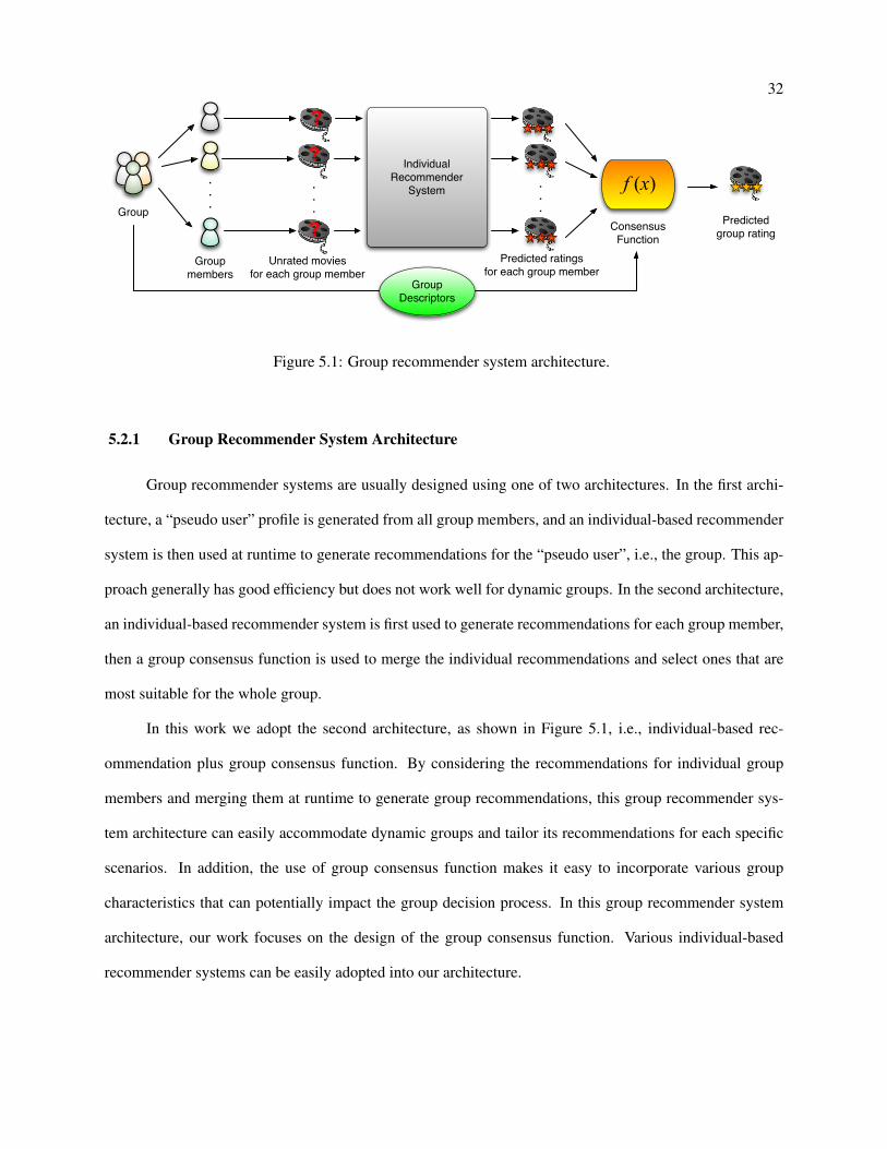
Figure 5.1: Group recommender system architecture.
5.2.1 Group Recommender System Architecture
Group recommender systems are usually designed using one of two architectures. In the first archi-
tecture, a “pseudo user” profile is generated from all group members, and an individual-based recommender
system is then used at runtime to generate recommendations for the “pseudo user”, i.e., the group. This ap-
proach generally has good efficiency but does not work well for dynamic groups. In the second architecture,
an individual-based recommender system is first used to generate recommendations for each group member,
then a group consensus function is used to merge the individual recommendations and select ones that are
most suitable for the whole group.
In this work we adopt the second architecture, as shown in Figure 5.1, i.e., individual-based rec-
ommendation plus group consensus function. By considering the recommendations for individual group
members and merging them at runtime to generate group recommendations, this group recommender sys-
tem architecture can easily accommodate dynamic groups and tailor its recommendations for each specific
scenarios. In addition, the use of group consensus function makes it easy to incorporate various group
characteristics that can potentially impact the group decision process. In this group recommender system
architecture, our work focuses on the design of the group consensus function. Various individual-based
recommender systems can be easily adopted into our architecture.

33Tom Mike G.
The Matrix 3 5 4
Star Wars 4 4 4
Table 5.1: Average satisfaction
5.2.2 Group Decision Strategies
Over the past decades, a variety of group decision strategies have been devised. One of the key
purposes of investigating group decision strategies is to understand how a group of individuals reach a
consensus, i.e., given individual preferences for an item, how does the group come up with a decision for
the item? To illustrate this, we review the three most common group decision strategies, including average
satisfaction, minimum misery, and maximum satisfaction.
Average Satisfaction: The most straightforward group decision strategy is to assume equal impor-
tance among all group members and compute the average satisfaction of the whole group for any given item.
Let n be the number of users in a group, ri,j be the rating of user j for item i, then the group rating for item
i is computed as follows:
GRi = average(ri,j) =
∑nj=1 ri,j
n(5.1)
Table 5.1 illustrates an example where the group preference for two different types of movies is consistent
with the average satisfaction (rating) of its group members.
Minimum Misery: Computing the average satisfaction within a group, though simple and straight-
forward, may not always be desirable. This happens when one or a few members really dislike an item, but
their low ratings for this item may be averaged out by higher ratings by other group members. For example,
Mike and Tom gave very different ratings to two horror movies (see Table 5.2). Tom really dislikes horror
movies and gave these two movies the lowest 1-star rating, whereas these two horror movies are acceptable
Tom Mike G.
The Shining 1 4 1
Drag Me to Hell 1 3 1
Table 5.2: Minimum misery

34Tom Mike G.
Harry Potter I 5 4 5
Harry Potter II 5 3 5
Table 5.3: Maximum satisfaction
for Mike. To please the least happy member (i.e., Tom in our example), the final decision of the group is to
rate each movie using the movie’s lowest rating among its group members, i.e., minimum misery:
GRi = min(ri,j) (5.2)
Maximum Satisfaction: In some scenarios, a group may choose to rate an item using the highest
rating among its group members. This happens when one or a few group members really like an item and
the remaining group members either agree or have reasonable satisfaction. As shown in Table 5.3, Tom is
highly interested in the Harry Potter movies and these movies are acceptable for Mike. Therefore, the final
decision of the group may reflect the highest rating within the group:
GRi = max(ri,j) (5.3)
While the three group decision strategies described above are most commonly used, none of them is
dominant across all groups [64]. It is unclear which group decision strategy should be applied under what
specific group characteristics. Next, we analyze in detail the different group characteristics and how they
lead to different group consensus functions.
5.3 System Description
Based on the group recommender system architecture and the three base group decision strategies,
we propose a group recommendation solution that fills the gap between specific group characteristics and
the dominant group decision strategy. Specifically, our solution consists of three key components: (a) group
descriptors that capture social, expertise, and dissimilarity information of a group; (b) a heuristic-based
group consensus function; and (c) a rule-based generic framework that automatically generates the most
suitable group consensus function for a group.

35Tom Nicole G.
Forrest Gump 5 3 5
Big Fish 4 2 4
Table 5.4: Strong social ties
5.3.1 Group Descriptors
As discussed above, different group decision strategies may be used, such as average satisfaction,
minimum misery, and maximum satisfaction. However, groups are diverse in nature and we show that
no single group decision strategy works best for all groups. To address this issue, we need to identify
the inherent characteristics of different groups and determine their specific impacts on the group decision
process. In this work, we investigate three crucial factors that affect a group’s decision and quantify these
three factors as the following group descriptors: social descriptor, expertise descriptor, and dissimilarity
descriptor.
Social Descriptor: We first investigate how the social factor affects a group’s decision. A group
consists of two or more individuals who are either directly or indirectly connected to each other by some
social relationships. Since they interact with and influence each other, the group decision is affected by the
strength of the social relationships. To illustrate this, let us consider the following examples. Suppose a
couple – Nicole and Tom1 – want to select a movie to watch together. The movie preferences for each of
them and the movie preferences for the couple (group) are listed in Table 5.4. An interesting observation is
that the couple’s final decision matches perfectly with the decision generated by the maximum satisfaction
strategy. Table 5.5 shows a different example. In this case, two acquaintances – Tom and John – have the
same movie preferences as the couple. However, the final decision that the acquaintances make is more
likely to correspond with the final decision generated by the average satisfaction strategy. Intuitively, the
1 The examples used in this chapter are based on real-world users, but user names are anonymized to protect privacy.
Tom John G.
Forrest Gump 5 3 4
Big Fish 4 2 3
Table 5.5: Weak social ties

36Contact Frequency (daily) < 0.2 0.2 ∼ 0.4 0.4 ∼ 0.6 0.6 ∼ 0.8 > 0.8
Social Level I II III IV V
Table 5.6: Categorization of social levels based on daily contact frequency.
difference between the two groups is the strength of their social relationships. Consequently, we believe that
the social relationship strength of a group should be taken into consideration in the group decision process.
The social descriptor is devised to measure the social relationship strength of a group. Intuitively, a
husband-and-wife family group usually has tighter and stronger social relationship than a group of people
who are merely acquaintances. For a two-member group, its social relationship can be easily defined as the
strength of the pairwise social link between the two members. In order to quantify the social relationship
strength of the pairwise member social link, we categorize the social relationship strength into five different
contact levels based on the average daily contact frequency between two members. These contact levels
are shown in Table 5.6. For example, the social strength of a family that consists of a husband and wife
is usually perfectly suitable for level 5 because they meet each other almost daily, while a faculty member
and his Ph.D. student may fit level 2 if they have regular meetings twice a week. To measure the social
relationship strength of a group with any number of members (at least two), we extend the two-member
social measure and define the social group descriptor as follows:
S(G) =2 ·∑1≤i<j≤|G|wi,j
|G| · (|G| − 1), (5.4)
where |G| is the size (number of members) of group G and wi,j is the social level between group members
i and j. Note that the social level is defined as zero if a pair of group members do not know each other.
Consider the example of a wedding ceremony where the groom’s friends may not know the bride’s friends
in advance. In this case, it is reasonable to consider their social levels to be zero.
Expertise Descriptor:
In addition to social relationship, another important factor that may affect a group’s decision is the
expertise of group members. To reach a consensus, the group decision process usually involves mild or
intense discussion. In this process, each group member is able to state his or her opinion based on the
experience that he or she has. In general, experts in a group are more talkative and may attempt to persuade

37Jack Bob G.
The Godfather 5 2 5
Goodfellas 5 2 4
Table 5.7: Expertise dominant
other group members. This can give rise to a situation where the final group decision is more inclined to
correspond with the decision of the experts in the group. For example, Jack and Bob want to select some
movies to watch together on a typical Saturday evening. As illustrated in Table 5.7, Bob does not have much
experience with gangster movies; therefore, he only gives two-star ratings to both of the movies. In contrast
with Bob, Jack has watched many gangster movies and has more experience with this type of movies (i.e.,
an expert); therefore, he persuades Bob to watch these two gangster movies with him. In this case, the
expertise factor, while it does not significantly influence Bob’s decision, dominates the final decision of the
group. Consequently, we believe that expertise is another important factor that should be taken into account
in the group decision process.
The expertise descriptor is devised to measure the relative expertise of individual group members. In
general, the opinions of experts may be weighted more heavily than those of other group members. Similar
to the strength of social relationships, we categorize the expertise of an individual into five levels. To divide
the expertise into different levels quantitatively, we define the expertise level based on the number of movies
that an individual has watched. Given a list of popular movies, the percentage of movies that an individual
has watched is divided into five different bins, as shown in Table 5.8. For example, given a movie list
containing 100 popular movies as well as a group consisting of four members, the number of movies that
the group members have watched is listed in Figure 5.2. We then compute the percentage of movies that each
group member has watched, and assign each group member into a specific bin to determine the expertise
level that an individual belongs to. For example, Jack has watched 67 movies out of 100 movies (i.e., 67%
Percentage of movies watched < 20% 20% ∼ 40% 40% ∼ 60% 60% ∼ 80% > 80%
Expertise Level I II III IV V
Table 5.8: Categorization of expertise levels based on percentage of movies watched.

38
Jack
Tom
Bob
Mike
0 20 40 60 80 100
# of watched movies
Figure 5.2: Number of movies watched by individual group members.
of movies in the 100-movie list), which means that his expertise belongs to the fourth level (60% – 80% of
movies has been watched). Recall that the expertise descriptor is intended to measure the relative expertise
of different group members. Therefore, we utilize the following equation to normalize the expertise levels
into the range from 0 to 1:
Ei(G) =ei
∑|G|j=1 ej
(5.5)
where Ei(G) is the normalized relative expertise level of group member i in group G, and ej is the absolute
expertise level of each group member j. Clearly, the sum of the relative expertise levels of a group is equal
to 1.
Dissimilarity Descriptor: Dissimilarity also influences the final decision of a group. As suggested
by Amer-Yahia et al. [19], dissimilarity should be considered in the context of a group decision strategy
because dissimilarity describes the disagreement between any two group members. Intuitively, the closer
the preference for an item between two members, the lower their disagreement for the item. In this work,
we therefore define the dissimilarity descriptor, which measures the preference difference among a group.
Here we use two metrics from [19], average pairwise dissimilarity (APD) and variance dissimilarity (VD),
to describe preference difference.
Given a group G and an item x, we define average pairwise dissimilarity as
APDx(G) =2
|G| · (|G| − 1)·∑
∀i,j∈G|ri,x − rj,x|, (5.6)

39
where |G| is the number of members in group G, and ri,x and rj,x denote item x’s ratings given by group
members i and j, respectively. Notice that i 6= j. As we can see, APDx(G) measures the average difference
of any two group members’ ratings for item x. For example, Table 5.4 and 5.5 show that Tom, Nicole, and
John’s ratings for the movie Forrest Gump are 5, 3, and 3. Using the average pairwise dissimilarity
metric, the dissimilarity descriptors for this movie and the 3-member group has a value of 1.333.
Another metric for the dissimilarity descriptor is variance dissimilarity, defined as
V Dx(G) =1
|G| ·∑
∀i∈G(ri,x − avgx)
2 (5.7)
where |G| is the number of members in group G, ri,x is group member i’s rating for item x, and avgx is
the mean of all individual members’ ratings for item x. This metric computes the mathematical variance of
the preferences for the item among group members. Let us return to the example of Tom, Nicole, and John
(see Table 5.4 and 5.5). Using the variance dissimilarity metric, we compute the dissimilarity descriptors
for the first movie, which equals to 0.889. Note that the two different dissimilarity metrics usually result in
different values.
5.3.2 A Heuristic Group Consensus Function
As discussed in Section 5.3.1, to choose the appropriate group decision strategy, we should take the
three factors – social factor, expertise factor and dissimilarity factor – into consideration. Here we propose
a heuristic group consensus function that incorporates all three factors in order to generate the final group
rating for a given group and a given item.
Recall the social descriptor is used to identify the social relationship strength of a group. Our obser-
vations of group dynamics suggest that when the social relationship strength is strong and tight, the final
decision that a group makes tends to reflect the maximum satisfaction of the group members. When the
social descriptor value is low (i.e., weak social ties), the final decision that a group makes tends to follow the
average satisfaction or minimum misery strategies. Unlike the social relationship descriptor, the expertise
descriptor is mainly used to apply a weight to each of the group members. A group member with more
expertise, and thus more influence, receives a higher weight than other group members with less expertise.
40
The dissimilarity descriptor mainly accounts for the fact that group members may not always have the same
tastes. Our experiments suggest that when a disagreement occurs in a group, the final decision that a group
makes reflects the level at which group members disagree with each other. Considering the three group
factors collectively, we combine these three descriptors into a heuristic group consensus function that uses
the three most common group decision strategies. Equation 5.8 quantifies the group decision strategy.
GRx = w1 · avg(Ei · ri,x) + w2 · (1− disx), if β < S < α
GRx = w1 ·max(Ei · ri,x) + w2 · (1− disx), if S > α
GRx = w1 ·min(Ei · ri,x) + w2 · (1− disx), if S < β
(5.8)
where disx represents the dissimilarity descriptors, which can be either average pairwise dissimilarity or
variance dissimilarity. w1 and w2 denote the relative importance of preference and dissimilarity in the final
decision, w1+w2 = 1. α and β are the thresholds that are used to identify the social relationship strength. As
indicated in Equation 5.8, we harness the social relationship strength to choose the group decision strategy.
Different social relationship strengths mean that a group makes its decision using different decision functions
– average satisfaction, minimum misery or maximum satisfaction. According to our experience, we assign
the threshold values for social relationship strength – α and β – 0.67 and 0.33 respectively. In addition,
Equation 5.8 also incorporates expertise weights (Ei) into each of the individual ratings (ri,x), and utilizes
two parameters to adjust the disagreement. Here, these two values for w1 and w2 (0.8 and 0.2, respectively)
are chosen after observing the data that we have collected from our user studies. An evaluation of this
equation is presented in Section 4.4.
5.3.3 Rule-Based Group Consensus Framework
While our results show that our heuristic group consensus function works well, it is developed based
on the specific cases we have observed. Ideally, we would like to develop a more general technique that
would be applicable not only for example to movies, but also to other data items and groups. Accordingly,
we have designed a generic framework that automatically analyzes group characteristics and generates the
corresponding group consensus function to predict group preferences. The basis for the design of this

41
framework is associative classification [56, 59]. In data mining and machine learning, classification involves
the construction of a model or classifier to predict categorical labels for data, such as “good” or “bad”. We
cast the group movie recommendation task as a classification task, where the goal is to predict a group
movie rating of 1, 2, 3, 4, or 5. Associative classification uses association rules to perform classification.
The following provides background on association rules and describes our general framework that uses
association rules to generate appropriate consensus functions for any group.
Our framework generates association rules by mining the training data set (e.g., from user studies).
Association rule mining is a popular method for discovering interesting relations or patterns between vari-
ables in a dataset [17, 18]. For example, if two group members individually rate a movie with a rating of
four, then this group of two also tends to agree on a group rating for four for this movie. This pattern can be
represented as the following association rule:
{minRating = 4} ∧ {maxRating = 4} ⇒ {groupRating = 4} (5.9)
To identify association rules, we must first search for frequent itemsets in the dataset. For example,
in the case of a transaction dataset for a supermarket, a set of items, such as bread and butter, that appear
frequently together in the dataset is a frequent itemset. In the simplified group movie rating example above,
{minRating = 4}, {maxRating = 4}, and {groupRating = 4} would be a frequent itemset. One
well-accepted algorithm for mining frequent itemsets is FP-growth [46]. FP-growth has been shown to be
an efficient and scalable method for mining both long and short frequent itemsets.
After finding frequent itemsets, we generate strong association rules from these frequent itemsets.
These strong association rules must satisfy minimum values for support and confidence. The support of
an association rule is defined as the percentage of transactions in the dataset containing all of the items in
the rule. The confidence of an association rule is defined as the percentage of transactions in the dataset,
containing the items in the rule, for which the rule is correct. More formally, for the rule A ⇒ B,
support(A ⇒ B) = P (A ∪B) (5.10)
confidence(A ⇒ B) = P (B|A) =support(A ∪B)
support(A)(5.11)

42Input: Dataset containing attributes and values for these attributes
Output: Associative classification rules
1 begin
2 for attribute ∈ dataset do
3 discretizedAttributes.add(discretize(attribute))4 end
5 for attribute ∈ discretizedAttributes do
6 newAttribute = NominalToBinominal(attribute)binomialAttributes.add(newAttribute)
7 end
8 frequentPatterns = FPGrowth(binomialAttributes);9 associationRules = AssociationRuleGenerator(frequentPatterns);
10 for associationRule ∈ associationRules do
11 lhs = associationRule.lhs();12 classifierRules.add(associationRule);13 if classifierRules.lhsMatch(lhs) then
14 classifierRules.removeLowestConfidence(lhs)15 end
16 end
17 end
Algorithm 2: Construct associative classification rules
The following describes Algorithm 2, which we use to mine association rules from the dataset ob-
tained from our user studies. First, we define meaningful attributes (items) in our data set. Based on our
experience with the user studies, we identify the following attributes: social strength (S), maximum group
member rating, minimum group member rating, average group member rating, standard deviation of mem-
ber ratings, average pairwise preference dissimilarity, average pairwise expertise dissimilarity, minimum
expertise, maximum expertise, expert member identifier, and group rating. We define expertise as an esti-
mate of the number of movies a group member has previously watched. The expert member identifier is
the identifier for the group member with the highest expertise. Average pairwise expertise dissimilarity is
defined as
EG,dissim =
∑
i,j∈G |eG,i − eG,j ||Pairs(G)| (5.12)
and average pairwise preference dissimilarity for item x is defined as
rx,G,dissim =
∑
i,j∈G |rx,G,i − rx,G,j ||Pairs(G)| (5.13)
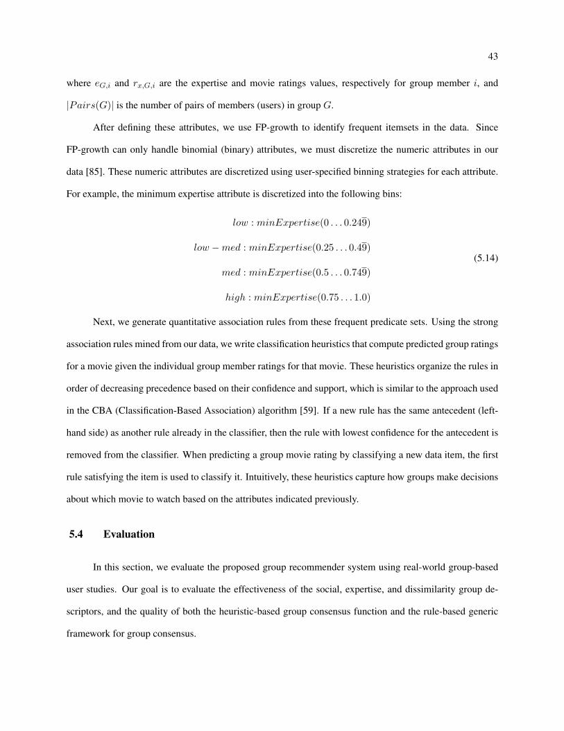
43
where eG,i and rx,G,i are the expertise and movie ratings values, respectively for group member i, and
|Pairs(G)| is the number of pairs of members (users) in group G.
After defining these attributes, we use FP-growth to identify frequent itemsets in the data. Since
FP-growth can only handle binomial (binary) attributes, we must discretize the numeric attributes in our
data [85]. These numeric attributes are discretized using user-specified binning strategies for each attribute.
For example, the minimum expertise attribute is discretized into the following bins:
low : minExpertise(0 . . . 0.249)
low −med : minExpertise(0.25 . . . 0.49)
med : minExpertise(0.5 . . . 0.749)
high : minExpertise(0.75 . . . 1.0)
(5.14)
Next, we generate quantitative association rules from these frequent predicate sets. Using the strong
association rules mined from our data, we write classification heuristics that compute predicted group ratings
for a movie given the individual group member ratings for that movie. These heuristics organize the rules in
order of decreasing precedence based on their confidence and support, which is similar to the approach used
in the CBA (Classification-Based Association) algorithm [59]. If a new rule has the same antecedent (left-
hand side) as another rule already in the classifier, then the rule with lowest confidence for the antecedent is
removed from the classifier. When predicting a group movie rating by classifying a new data item, the first
rule satisfying the item is used to classify it. Intuitively, these heuristics capture how groups make decisions
about which movie to watch based on the attributes indicated previously.
5.4 Evaluation
In this section, we evaluate the proposed group recommender system using real-world group-based
user studies. Our goal is to evaluate the effectiveness of the social, expertise, and dissimilarity group de-
scriptors, and the quality of both the heuristic-based group consensus function and the rule-based generic
framework for group consensus.

44
5.4.1 Participants and Groups
From 2009 to 2010, we have recruited 10 groups (32 individuals) to participate in our user studies.
All participants are college or graduate students with an approximate average age of 28. For each group,
individual group members are asked to describe his or her social relationships with other members in the
group. The social relationships between two peers mainly contain the following four types of relationships:
couple, close friends, acquaintances and first acquaintances (a group whose members are meeting each other
for the first time). The strength of these four social relationships are sequentially decreasing. Additionally,
in order to quantify the strength of their social relationship, each of the participants is asked to provide
his or her contact frequency with other group members (i.e., how frequently the participant interacts with
other group members). Based on these reported social relationships, we categorize the 10 groups into four
different types: four couple groups (with two members per group), two close-friend groups (three members
per group), three acquaintance groups (two members per group) and one first-acquaintance group with 12
members.
We believe the composition of our groups is representative of many scenarios in the real world.
Typically, a first-acquaintance group is fairly large, such as a group in college student orientation in which
group members do not know each other very well. On the other hand, groups with strong relationships are
usually relatively small, since it is difficult for all group members to know each other in a large group. For
example, at a party some people may know a majority of their fellow partygoers, whereas others may not.
Though our user studies can represent many groups in the real world, there are a few cases that we have not
investigated, such as a very large group where classmates know each other to varying degrees (e.g. a big
high school class). We plan to continue investigating more diverse groups, including very large groups.
5.4.2 Experimental Methodology
The goal of our user studies is to collect information regarding social relationships, movie preferences,
and expertise levels for the members of each group and then utilize this data to evaluate the performance
of our proposed group consensus functions. To obtain the movie preferences and expertise levels of each

45
1
2
3
4
5
0 1 2 3 4 5 6 7 8 9 10 11 12 13 14 15 16 17 18 19 20
Movie
Rating
Movie ID
User 1 User 2 Group
Figure 5.3: Individual ratings vs. group rating in a regular group.
participant, we selected 20 movies out of the top 250 popular movies from IMDB [8]. For our study, it
is impractical to select the 20 movies from the pool randomly, since random selection may give rise to a
situation in which the selected movies may all belong to a small set of genres. For example, the 20 selected
movies may belong to only two genres – horror and science fiction. In this case, the expertise levels that we
collect from our participants may contain a strong bias, since it is possible that some participants are big fans
of horror movies or science-fiction movies and have watched a lot of movies in these genres, but they cannot
be considered as movie experts in all movie genres. To avoid this potential bias, we select the movies used
for our user study across 10 different movie genres including Action, Comedy, Crime, Family, Horror,
Science Fiction, Thriller, Romance and War. In our study, each movie genre contains two movies.
Asking each participant to view all 20 movies and provide ratings for each movie is impractical.
Instead, we ask each participant to watch the trailers of these 20 movies, because each trailer is usually 2∼3
minutes long. A previous study has indicated that using movie trailers to capture people’s preferences is
realistic and efficient [83]. All participants are instructed to provide ratings on a scale of 1 to 5 (1 being
the worst and 5 being the most favorite) for these 20 movie trailers according to their movie preferences. In
addition, for the purpose of expertise information collection, we ask participants to identify those movies that
they have previously watched. Since the study is conducted in an independent environment (i.e., making
personal decision without discussion and interruption), we believe that the ratings that each participant
provides for us correctly represent the movie preferences of the participant. After we collect the movie
preferences of each participant, the participants are asked to return to their groups and begin discussion about
these 20 movie trailers. The purpose of this discussion is to provide group ratings for the movies. Intuitively,

46
Figure 5.4: Still frame from 12-person group user study, showing group members discussing their opinions
about a movie.
group ratings are quite diverse and may not have correlations with each group member, regardless of the size
of the group (see Figure 5.3). Both the group ratings from the 10 groups and the participants’ individual
ratings are used for verifying our group consensus functions. Figure 5.4 shows a video still frame from our
12-person user study. This still frame was captured soon after the group had finished watching a movie
trailer and provided their individual ratings, and shows the group members discussing their opinions about
the movie.
5.4.3 Evaluation Measures
In the context of prediction, Root Mean Square Error (RMSE) is a widely used evaluation metric.
RMSE measures the differences between values predicted by a model and the values actually observed from
the process or entity being modeled. It is generally accepted as a good measure of precision. In our setting,
we are interested in the precision of our prediction with respect to movie ratings provided by a given group.
RMSE can be formalized as follows:
Given two vectors, where the first vector contains the actual group ratings for n movies, called ground
truth, GT = [r1, r2, ..., rn], and the second vector contains predicted group ratings for n movies, PR =

47
[r′1, r′2, ..., r
′n], RMSE is calculated by the following equation
RMSE =
√
∑ni=1(ri − r′i)
2
n(5.15)
When the predicted group ratings are very close to the actual group ratings, the value of ri − r′i is close to
zero, and the RMSE is also close to zero. Therefore, smaller RMSE values indicate better predictions.
One other measure we use for evaluation is Pearson product-moment correlation coefficient [74] ,
which measures the correlation between two variables X and Y .
corr =
∑ni=1(Xi −X) · (Yi − Y )
(n− 1) · σX · σY, (5.16)
where σX and σY are standard deviation of variable X and Y , respectively. A value close to 1.0 indicates
strong positive correlation between the two variables; a value close to -1.0 indicates strong negative cor-
relation, and a value close to 0 indicates low correlation. Therefore, we harness the Pearson correlation
coefficient to investigate which group members or characteristics dominate a group’s decision.
5.4.4 Experimental Results
The purpose of our real-world user study based experiments is to help us to answer the following
questions:
(1) Is the group decision process affected by the group’s social and expertise characteristics?
(2) Is there a general group consensus function (i.e., group decision model) that can capture the group
behaviors?
(3) If there is a group consensus function that captures group behaviors, can it be applied to all groups
or a majority of groups?
(4) How well do our heuristic-based and rule-based group decision models, or consensus functions,
perform in comparison to a state-of-the-art group decision model [19]?
We first evaluate the impact of members’ expertise on a group’s decision. Figure 5.5 shows, for a
two-member group in our study, individual members’ ratings and group ratings for the 20 movies we have
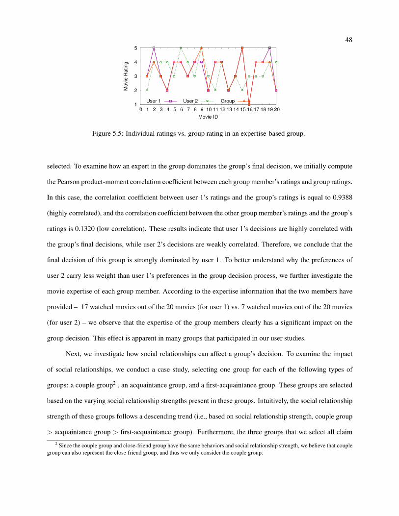
48
1
2
3
4
5
0 1 2 3 4 5 6 7 8 9 10 11 12 13 14 15 16 17 18 19 20
Movie
Rating
Movie ID
User 1 User 2 Group
Figure 5.5: Individual ratings vs. group rating in an expertise-based group.
selected. To examine how an expert in the group dominates the group’s final decision, we initially compute
the Pearson product-moment correlation coefficient between each group member’s ratings and group ratings.
In this case, the correlation coefficient between user 1’s ratings and the group’s ratings is equal to 0.9388
(highly correlated), and the correlation coefficient between the other group member’s ratings and the group’s
ratings is 0.1320 (low correlation). These results indicate that user 1’s decisions are highly correlated with
the group’s final decisions, while user 2’s decisions are weakly correlated. Therefore, we conclude that the
final decision of this group is strongly dominated by user 1. To better understand why the preferences of
user 2 carry less weight than user 1’s preferences in the group decision process, we further investigate the
movie expertise of each group member. According to the expertise information that the two members have
provided – 17 watched movies out of the 20 movies (for user 1) vs. 7 watched movies out of the 20 movies
(for user 2) – we observe that the expertise of the group members clearly has a significant impact on the
group decision. This effect is apparent in many groups that participated in our user studies.
Next, we investigate how social relationships can affect a group’s decision. To examine the impact
of social relationships, we conduct a case study, selecting one group for each of the following types of
groups: a couple group2 , an acquaintance group, and a first-acquaintance group. These groups are selected
based on the varying social relationship strengths present in these groups. Intuitively, the social relationship
strength of these groups follows a descending trend (i.e., based on social relationship strength, couple group
> acquaintance group > first-acquaintance group). Furthermore, the three groups that we select all claim
2 Since the couple group and close-friend group have the same behaviors and social relationship strength, we believe that couple
group can also represent the close friend group, and thus we only consider the couple group.

49
similar member expertise within a group, thus the expertise factor does not have impact on the group decision
process.
To understand how social relationship affects a group’s decision, we use three of the most common
group decision strategies, average satisfaction, minimum misery, and maximum satisfaction, to predict the
group decision, and then compare the predicted ratings with the actual group ratings (ground truth) by com-
puting the Pearson correlation coefficient between each prediction and the ground truth. For the couple
group, the computed Pearson correlation values of the three decision strategies are 0.7393 (average satisfac-
tion), 0.8324 (maximum satisfaction) and 0.4866 (minimum misery). As we can see from these results, of
the three decision strategies, the group rating predicted by maximum satisfaction has the highest correlation
with the actual group decision. Therefore, we conclude that the maximum satisfaction strategy captures the
group decision of the couple group relatively well. Similar to the couple group, the acquaintance group also
consists of two group members. In contrast to the couple group, the members in the acquaintance group have
a weaker social relationship. Furthermore, the values of the Pearson correlations for the acquaintance group
also differ from the values for the couple group. For the acquaintance group, the values of Pearson correla-
tion are 0.9290 (average satisfaction), 0.8386 (maximum satisfaction), and 0.8693 (minimum misery). We
observe that the performance of the average satisfaction strategy exceeds the other two strategies. Finally,
we also compute the Pearson correlation values for the first-acquaintance group, which consists of 12 group
members. The Pearson correlation values for this group are 0.5927 (average satisfaction), 0.1808 (most
satisfaction), and 0.9485 (minimum misery). In this case, the best decision strategy is the minimum misery
strategy. Observing the three groups and the variation in their Pearson correlation values, we conclude that
a decrease in the social relationship strength results in a variation in group decision strategy. Based on the
data from our user studies, we conclude that a group with a strong social relationship tends to maximize
the satisfaction of a user in the group, while a group with a weak social relationship tends to minimize the
misery of a user in the group.
We next investigate whether our heuristic group consensus function that combines the social, exper-
tise, and dissimilarity descriptors (described in Section 5.3.2) can accurately predict a group’s decision. Here
we use a state-of-the-art group decision model [19] as the baseline for comparison with our group consensus
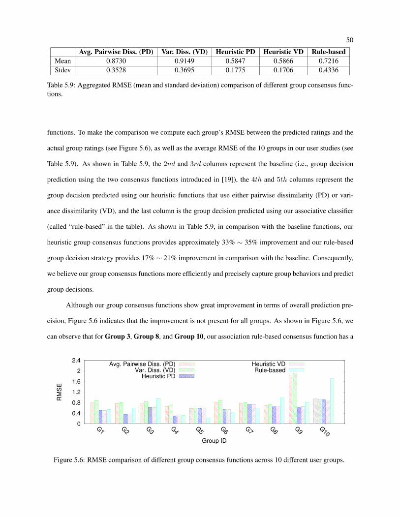
50
Avg. Pairwise Diss. (PD) Var. Diss. (VD) Heuristic PD Heuristic VD Rule-based
Mean 0.8730 0.9149 0.5847 0.5866 0.7216
Stdev 0.3528 0.3695 0.1775 0.1706 0.4336
Table 5.9: Aggregated RMSE (mean and standard deviation) comparison of different group consensus func-
tions.
functions. To make the comparison we compute each group’s RMSE between the predicted ratings and the
actual group ratings (see Figure 5.6), as well as the average RMSE of the 10 groups in our user studies (see
Table 5.9). As shown in Table 5.9, the 2nd and 3rd columns represent the baseline (i.e., group decision
prediction using the two consensus functions introduced in [19]), the 4th and 5th columns represent the
group decision predicted using our heuristic functions that use either pairwise dissimilarity (PD) or vari-
ance dissimilarity (VD), and the last column is the group decision predicted using our associative classifier
(called “rule-based” in the table). As shown in Table 5.9, in comparison with the baseline functions, our
heuristic group consensus functions provides approximately 33% ∼ 35% improvement and our rule-based
group decision strategy provides 17% ∼ 21% improvement in comparison with the baseline. Consequently,
we believe our group consensus functions more efficiently and precisely capture group behaviors and predict
group decisions.
Although our group consensus functions show great improvement in terms of overall prediction pre-
cision, Figure 5.6 indicates that the improvement is not present for all groups. As shown in Figure 5.6, we
can observe that for Group 3, Group 8, and Group 10, our association rule-based consensus function has a
0
0.4
0.8
1.2
1.6
2
2.4
G1
G2
G3
G4
G5
G6
G7
G8
G9
G10
RM
SE
Group ID
Avg. Pairwise Diss. (PD)Var. Diss. (VD)
Heuristic PD
Heuristic VDRule-based
Figure 5.6: RMSE comparison of different group consensus functions across 10 different user groups.
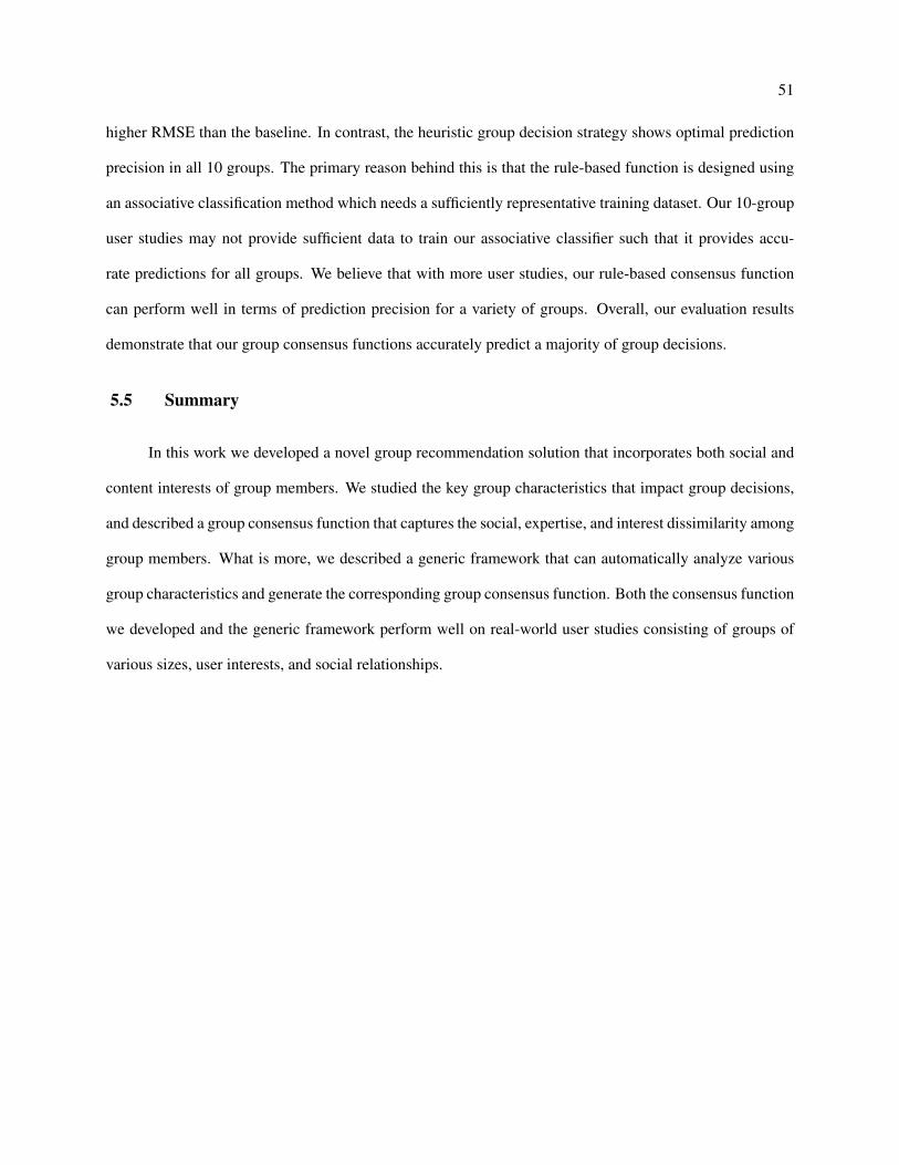
51
higher RMSE than the baseline. In contrast, the heuristic group decision strategy shows optimal prediction
precision in all 10 groups. The primary reason behind this is that the rule-based function is designed using
an associative classification method which needs a sufficiently representative training dataset. Our 10-group
user studies may not provide sufficient data to train our associative classifier such that it provides accu-
rate predictions for all groups. We believe that with more user studies, our rule-based consensus function
can perform well in terms of prediction precision for a variety of groups. Overall, our evaluation results
demonstrate that our group consensus functions accurately predict a majority of group decisions.
5.5 Summary
In this work we developed a novel group recommendation solution that incorporates both social and
content interests of group members. We studied the key group characteristics that impact group decisions,
and described a group consensus function that captures the social, expertise, and interest dissimilarity among
group members. What is more, we described a generic framework that can automatically analyze various
group characteristics and generate the corresponding group consensus function. Both the consensus function
we developed and the generic framework perform well on real-world user studies consisting of groups of
various sizes, user interests, and social relationships.

Chapter 6
A Large-scale Study of Group Viewing Preferences
Having investigated how social and content interests impact group preferences with a small-scale
study presented in Chapter 5, in this chapter we turn to an analysis of group preferences using a large-scale
dataset [29]. We also present a simple group recommendation model that captures the group preference
patterns apparent from our study.
6.1 Overview
We are in the midst of an industry-wide shift, wherein the primary means of home broadcast video
entertainment is moving from traditional television sets to online and Web services (e.g., Netflix, Hulu, and
Xbox) that contain a rapidly expanding catalogue of content. While there is a substantial body of work on
understanding the preferences of individuals in these settings—largely for the purpose of aiding users in
discovering relevant and novel content within these catalogues—there is a comparatively small amount of
research on modeling group viewing habits, mostly owing to the difficulty of collecting co-viewing data.
Absent this data, group preferences are often modeled via simple aggregates of the underlying individual
preferences. While such approaches are somewhat successful, they obscure more subtle group dynamics and
interactions that affect group decision making—for instance, the preferences of a parent and child together
may be difficult to determine from what each watches alone.
As reviewed in Chapter 3, previous studies often rely on small-scale, self-reported viewing data to
draw qualitative conclusions about group viewing, and most existing large-scale log datasets contain group
preference data for only several hundred groups [81, 76]. In contrast, we use a dataset that contains both
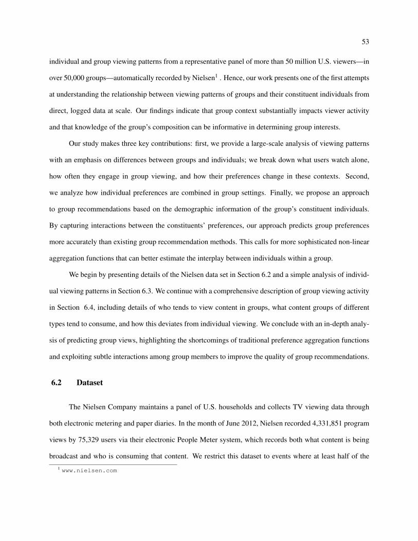
53
individual and group viewing patterns from a representative panel of more than 50 million U.S. viewers—in
over 50,000 groups—automatically recorded by Nielsen1 . Hence, our work presents one of the first attempts
at understanding the relationship between viewing patterns of groups and their constituent individuals from
direct, logged data at scale. Our findings indicate that group context substantially impacts viewer activity
and that knowledge of the group’s composition can be informative in determining group interests.
Our study makes three key contributions: first, we provide a large-scale analysis of viewing patterns
with an emphasis on differences between groups and individuals; we break down what users watch alone,
how often they engage in group viewing, and how their preferences change in these contexts. Second,
we analyze how individual preferences are combined in group settings. Finally, we propose an approach
to group recommendations based on the demographic information of the group’s constituent individuals.
By capturing interactions between the constituents’ preferences, our approach predicts group preferences
more accurately than existing group recommendation methods. This calls for more sophisticated non-linear
aggregation functions that can better estimate the interplay between individuals within a group.
We begin by presenting details of the Nielsen data set in Section 6.2 and a simple analysis of individ-
ual viewing patterns in Section 6.3. We continue with a comprehensive description of group viewing activity
in Section 6.4, including details of who tends to view content in groups, what content groups of different
types tend to consume, and how this deviates from individual viewing. We conclude with an in-depth analy-
sis of predicting group views, highlighting the shortcomings of traditional preference aggregation functions
and exploiting subtle interactions among group members to improve the quality of group recommendations.
6.2 Dataset
The Nielsen Company maintains a panel of U.S. households and collects TV viewing data through
both electronic metering and paper diaries. In the month of June 2012, Nielsen recorded 4,331,851 program
views by 75,329 users via their electronic People Meter system, which records both what content is being
broadcast and who is consuming that content. We restrict this dataset to events where at least half of the
1 www.nielsen.com
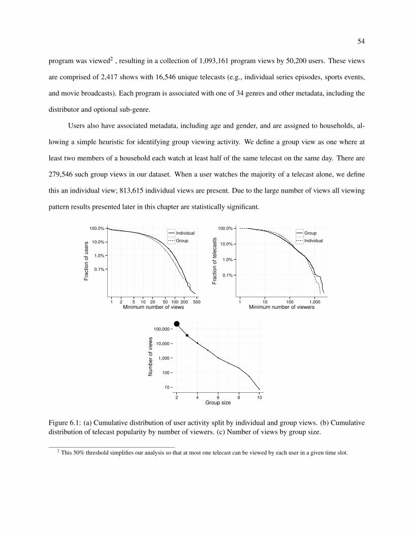
54
program was viewed2 , resulting in a collection of 1,093,161 program views by 50,200 users. These views
are comprised of 2,417 shows with 16,546 unique telecasts (e.g., individual series episodes, sports events,
and movie broadcasts). Each program is associated with one of 34 genres and other metadata, including the
distributor and optional sub-genre.
Users also have associated metadata, including age and gender, and are assigned to households, al-
lowing a simple heuristic for identifying group viewing activity. We define a group view as one where at
least two members of a household each watch at least half of the same telecast on the same day. There are
279,546 such group views in our dataset. When a user watches the majority of a telecast alone, we define
this an individual view; 813,615 individual views are present. Due to the large number of views all viewing
pattern results presented later in this chapter are statistically significant.
0.1%
1.0%
10.0%
100.0%
1 2 5 10 20 50 100 200 500
Minimum number of views
Fra
ction o
f users
Individual
Group
0.1%
1.0%
10.0%
100.0%
1 10 100 1,000
Minimum number of viewers
Fra
ction o
f te
lecasts
Group
Individual
●
●
●
●
●
●
●
●
●10
100
1,000
10,000
100,000
2 4 6 8 10
Group size
Num
ber
of vie
ws
Figure 6.1: (a) Cumulative distribution of user activity split by individual and group views. (b) Cumulative
distribution of telecast popularity by number of viewers. (c) Number of views by group size.
2 This 50% threshold simplifies our analysis so that at most one telecast can be viewed by each user in a given time slot.
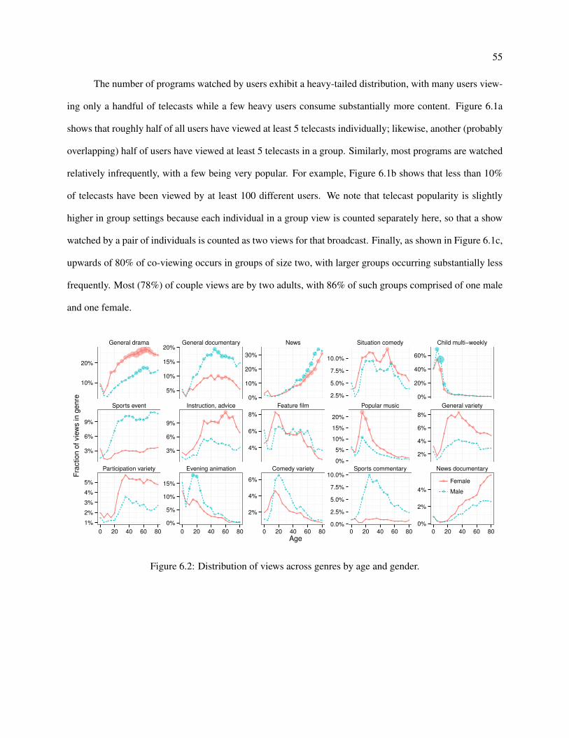
55
The number of programs watched by users exhibit a heavy-tailed distribution, with many users view-
ing only a handful of telecasts while a few heavy users consume substantially more content. Figure 6.1a
shows that roughly half of all users have viewed at least 5 telecasts individually; likewise, another (probably
overlapping) half of users have viewed at least 5 telecasts in a group. Similarly, most programs are watched
relatively infrequently, with a few being very popular. For example, Figure 6.1b shows that less than 10%
of telecasts have been viewed by at least 100 different users. We note that telecast popularity is slightly
higher in group settings because each individual in a group view is counted separately here, so that a show
watched by a pair of individuals is counted as two views for that broadcast. Finally, as shown in Figure 6.1c,
upwards of 80% of co-viewing occurs in groups of size two, with larger groups occurring substantially less
frequently. Most (78%) of couple views are by two adults, with 86% of such groups comprised of one male
and one female.
General drama General documentary News Situation comedy Child multi−weekly
Sports event Instruction, advice Feature film Popular music General variety
Participation variety Evening animation Comedy variety Sports commentary News documentary
10%
20%
5%
10%
15%
20%
0%
10%
20%
30%
2.5%
5.0%
7.5%
10.0%
0%
20%
40%
60%
3%
6%
9%
3%
6%
9%
4%
6%
8%
0%
5%
10%
15%
20%
2%
4%
6%
8%
1%
2%
3%
4%
5%
0%
5%
10%
15%
2%
4%
6%
0.0%
2.5%
5.0%
7.5%
10.0%
0%
2%
4%
0 20 40 60 80 0 20 40 60 80 0 20 40 60 80 0 20 40 60 80 0 20 40 60 80
Age
Fra
ction o
f vie
ws in g
enre
Female
Male
Figure 6.2: Distribution of views across genres by age and gender.
56
Table 6.1: Ranked list of genres for individuals with varying demographics.
Male child Female teen Male adult Female adult Male senior Female senior
Child multi-weekly Popular music General documentary General drama News General drama
General drama General drama General drama General documentary General drama News
Feature film Child multi-weekly Sports event Situation comedy General documentary General documentary
General documentary Situation comedy Situation comedy Instruction, advice Sports event Instruction, advice
Evening animation Feature film Feature film News Situation comedy Situation comedy
Sports event Evening animation News General variety Instruction, advice Participation variety
Situation comedy General documentary Instruction, advice Participation variety Feature film General variety
Popular music General variety Evening animation Feature film Participation variety Sports event
Participation variety Comedy variety Participation variety Popular music News documentary News documentary
Instruction, advice Instruction, advice Sports commentary Sports event General variety Feature film
6.3 Individual Viewing Patterns
In this section, we analyze how individual viewing behavior varies with age and gender. For this
purpose, we compute the genre-specific view counts in the context of demographic information. Figure 6.2
depicts how users of varying age and gender distribute their attention across genres at the aggregate level.
Panels are ordered by decreasing overall genre popularity, and point size shows the relative fraction of overall
views accounted for by each demographic group in each genre. Table 6.1 provides an alternative view of
these data, showing the top genres by view count for individuals of different age and gender. We discuss
several clear age and gender patterns below. Note that these viewing patterns are limited to individual views
only.
We observe strong age effects for the viewing of certain genres like general drama, child multi-weekly,
evening animation, news, popular music, general variety and news documentary. For instance, we observe
that older viewers spend a large fraction (about 20-30%) of their time watching news relative to teenagers,
who consume little of this genre and devote substantially more of their attention to popular music shows.
Likewise, general documentaries are more popular with adults and seniors than with children, while child
multi-weekly programs are popular for children and much less popular with adults and seniors, as one would
expect. General dramas are quite popular for every age and gender demographic we examined.
We also see gender differences in individual preferences, with females spending more of their time
watching talk shows, drama, and music relative to males, who prefer animation, documentaries, and sports.
Sports events tend to be more popular with males than with females, across all ages.
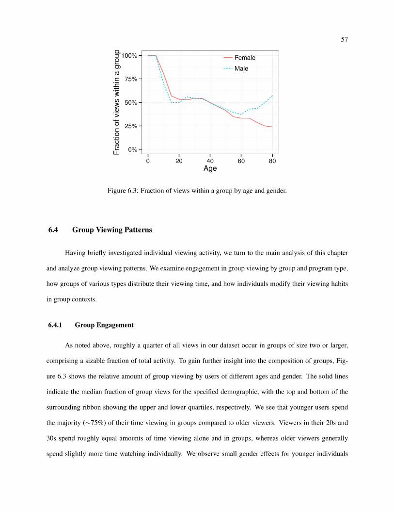
57
0%
25%
50%
75%
100%
0 20 40 60 80
Age
Fra
ction o
f vie
ws w
ithin
a g
roup
Female
Male
Figure 6.3: Fraction of views within a group by age and gender.
6.4 Group Viewing Patterns
Having briefly investigated individual viewing activity, we turn to the main analysis of this chapter
and analyze group viewing patterns. We examine engagement in group viewing by group and program type,
how groups of various types distribute their viewing time, and how individuals modify their viewing habits
in group contexts.
6.4.1 Group Engagement
As noted above, roughly a quarter of all views in our dataset occur in groups of size two or larger,
comprising a sizable fraction of total activity. To gain further insight into the composition of groups, Fig-
ure 6.3 shows the relative amount of group viewing by users of different ages and gender. The solid lines
indicate the median fraction of group views for the specified demographic, with the top and bottom of the
surrounding ribbon showing the upper and lower quartiles, respectively. We see that younger users spend
the majority (∼75%) of their time viewing in groups compared to older viewers. Viewers in their 20s and
30s spend roughly equal amounts of time viewing alone and in groups, whereas older viewers generally
spend slightly more time watching individually. We observe small gender effects for younger individuals
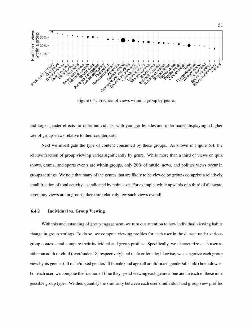
58
●
●● ●
●
●
●
●
●
●
●
●
●● ●●
●
●
●
●
●
●●
●
●
●●
●
●
●
●
●
●●
10%
20%
30%
Partic
ipat
ion
varie
ty
Quiz pa
nel
Day
time
dram
a
Quiz give
away
Official p
olice
Dev
otiona
l
Awar
d ce
rem
onies
Child m
ulti−
wee
kly
Sports
eve
nt
Audienc
e pa
rticipa
tion
Suspe
nse/
mys
tery
Feat
ure
film
New
s do
cum
enta
ry
Adven
ture
Gen
eral d
ram
a
Con
vers
ations
, colloqu
ies
Gen
eral d
ocum
enta
ry
Com
edy va
riety
Gen
eral var
iety
Situat
ion
com
edy
Sports
new
s
Instru
ction,
adv
ice
Evening
anim
ation
Scien
ce fiction
Form
at var
ies
Popular
mus
ic
Con
cert
mus
ic
New
s
Privat
e de
tective
Wes
tern
dra
ma
Unc
lass
ified
Sports
ant
hology
Sports
com
men
tary
Politica
l
Fra
ctio
n o
f vie
ws
with
in a
gro
up
Figure 6.4: Fraction of views within a group by genre.
and larger gender effects for older individuals, with younger females and older males displaying a higher
rate of group views relative to their counterparts.
Next we investigate the type of content consumed by these groups. As shown in Figure 6.4, the
relative fraction of group viewing varies significantly by genre. While more than a third of views on quiz
shows, drama, and sports events are within groups, only 20% of music, news, and politics views occur in
groups settings. We note that many of the genres that are likely to be viewed by groups comprise a relatively
small fraction of total activity, as indicated by point size. For example, while upwards of a third of all award
ceremony views are in groups, there are relatively few such views overall.
6.4.2 Individual vs. Group Viewing
With this understanding of group engagement, we turn our attention to how individual viewing habits
change in group settings. To do so, we compute viewing profiles for each user in the dataset under various
group contexts and compare their individual and group profiles. Specifically, we characterize each user as
either an adult or child (over/under 18, respectively) and male or female; likewise, we categorize each group
view by its gender (all male/mixed gender/all female) and age (all adult/mixed gender/all child) breakdowns.
For each user, we compute the fraction of time they spend viewing each genre alone and in each of these nine
possible group types. We then quantify the similarity between each user’s individual and group view profiles
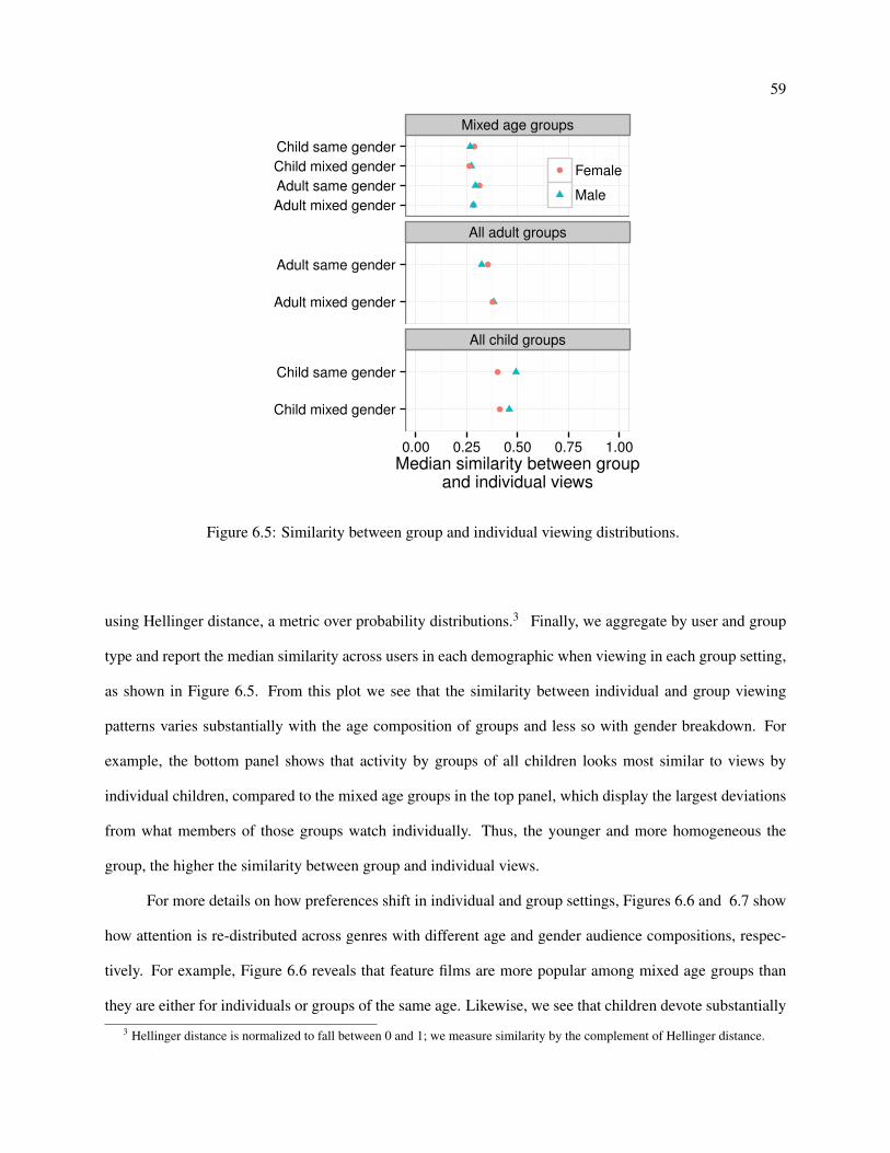
59
●
●
●
●
●
●
●
●
Mixed age groups
All adult groups
All child groups
Adult mixed gender
Adult same gender
Child mixed gender
Child same gender
Adult mixed gender
Adult same gender
Child mixed gender
Child same gender
0.00 0.25 0.50 0.75 1.00
Median similarity between groupand individual views
● Female
Male
Figure 6.5: Similarity between group and individual viewing distributions.
using Hellinger distance, a metric over probability distributions.3 Finally, we aggregate by user and group
type and report the median similarity across users in each demographic when viewing in each group setting,
as shown in Figure 6.5. From this plot we see that the similarity between individual and group viewing
patterns varies substantially with the age composition of groups and less so with gender breakdown. For
example, the bottom panel shows that activity by groups of all children looks most similar to views by
individual children, compared to the mixed age groups in the top panel, which display the largest deviations
from what members of those groups watch individually. Thus, the younger and more homogeneous the
group, the higher the similarity between group and individual views.
For more details on how preferences shift in individual and group settings, Figures 6.6 and 6.7 show
how attention is re-distributed across genres with different age and gender audience compositions, respec-
tively. For example, Figure 6.6 reveals that feature films are more popular among mixed age groups than
they are either for individuals or groups of the same age. Likewise, we see that children devote substantially
3 Hellinger distance is normalized to fall between 0 and 1; we measure similarity by the complement of Hellinger distance.
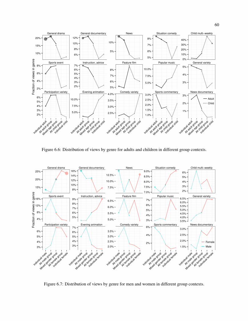
60
General drama General documentary News Situation comedy Child multi−weekly
Sports event Instruction, advice Feature film Popular music General variety
Participation variety Evening animation Comedy variety Sports commentary News documentary
10%
15%
20%
6%
8%
10%
12%
5%
10%
5%
6%
7%
8%
0%
10%
20%
30%
40%
2%
4%
6%
8%
2%
3%
4%
5%
6%
7%
5%
6%
7%
8%
5.0%
7.5%
10.0%
3%
4%
5%
2%
3%
4%
5%
6%
5.0%
7.5%
10.0%
2.5%
3.0%
3.5%
4.0%
1.0%
1.5%
2.0%
2.5%
3.0%
1%
2%
3%
Individu
al a
dult
All ad
ult g
roup
Mixed
age
gro
up
All ch
ild g
roup
Individu
al child
Individu
al a
dult
All ad
ult g
roup
Mixed
age
gro
up
All ch
ild g
roup
Individu
al child
Individu
al a
dult
All ad
ult g
roup
Mixed
age
gro
up
All ch
ild g
roup
Individu
al child
Individu
al a
dult
All ad
ult g
roup
Mixed
age
gro
up
All ch
ild g
roup
Individu
al child
Individu
al a
dult
All ad
ult g
roup
Mixed
age
gro
up
All ch
ild g
roup
Individu
al child
Fra
ction o
f vie
ws in g
enre
Adult
Child
Figure 6.6: Distribution of views by genre for adults and children in different group contexts.
General drama General documentary News Situation comedy Child multi−weekly
Sports event Instruction, advice Feature film Popular music General variety
Participation variety Evening animation Comedy variety Sports commentary News documentary
15%
20%
25%
8%
10%
12%
14%
16%
7.5%
10.0%
12.5%
7.0%
7.5%
8.0%
8.5%
9.0%
2%
3%
4%
5%
6%
4%
8%
12%
16%
5%
6%
7%
8%
9%
5.0%
5.5%
6.0%
6.5%
3%
4%
5%
6%
7%
3.5%
4.0%
4.5%
5.0%
5.5%
6.0%
6.5%
3%
4%
5%
6%
3%
4%
5%
6%
7%
2.0%
2.5%
3.0%
3.5%
2%
4%
6%
1.5%
2.0%
2.5%
3.0%
Individu
al m
ale
All m
ale
grou
p
Mixed
gen
der g
roup
All fe
male
grou
p
Individu
al fe
male
Individu
al m
ale
All m
ale
grou
p
Mixed
gen
der g
roup
All fe
male
grou
p
Individu
al fe
male
Individu
al m
ale
All m
ale
grou
p
Mixed
gen
der g
roup
All fe
male
grou
p
Individu
al fe
male
Individu
al m
ale
All m
ale
grou
p
Mixed
gen
der g
roup
All fe
male
grou
p
Individu
al fe
male
Individu
al m
ale
All m
ale
grou
p
Mixed
gen
der g
roup
All fe
male
grou
p
Individu
al fe
male
Fra
ction o
f vie
ws in g
enre
Female
Male
Figure 6.7: Distribution of views by genre for men and women in different group contexts.

61
more of their time to child multi-weekly shows when viewing in groups (∼50%) compared to viewing alone
(∼30%). Adults watch more dramas, documentaries, and sports events in groups with other adults, and
are more likely to watch news, sports commentary, and advice shows alone. We also see that adults and
children both compromise on certain genres: one group watching more than usual and the other watching
less. This occurs for many genres, including dramas and documentaries, where adults watch less than usual
and children watch more, as well as popular music and evening animation, where children watch less and
adult watch more together than they do separately. We see little compromise for adults on sports events and
participation shows, possibly due to time sensitivity; in both of these cases, adults watch just as much as
they do in groups with other adults, and children watch far more than they otherwise would.
We also see substantial shifts in preferences as gender composition varies in Figure 6.7. For instance,
feature films are more popular with same gender groups than they are with either individuals or mixed
gender groups, whereas the opposite effect is seen for news, which is more popular amongst individual
males and females than in groups. We also see that news is more popular in mixed gender groups than in
same-gender groups. We speculate that this effect is attributed to passive viewing patterns of couples in
the same household, rather than an active desire to watch news as a group. While these changes are fairly
similar between men and women, we note that other genres show gender-specific effects. For example,
groups of men spend nearly double the amount of their time watching sports compared to individual males,
but no such difference is seen for females. Likewise, all female groups spend substantially more of their
time viewing popular music shows than do individual females. Finally, as with age effects, mixed gender
groups appear to compromise on many categories. For dramas, advice, and sitcoms, men watch more and
women watch less together than when in homogeneous groups. We see the reverse effect for documentaries,
evening animation, and sports shows, with women watching more and men watching less.
Table 6.2, which shows a rank-ordered list of the most popular genres by audience type, provides
a complementary perspective on this variation in preferences. For example, we see that while individual
and groups of adults prefer to watch drama, news, and documentaries, children prefer multi-weekly shows,
animation, and popular music; mixed age groups display a non-trivial blend of these preferences. Similarly,
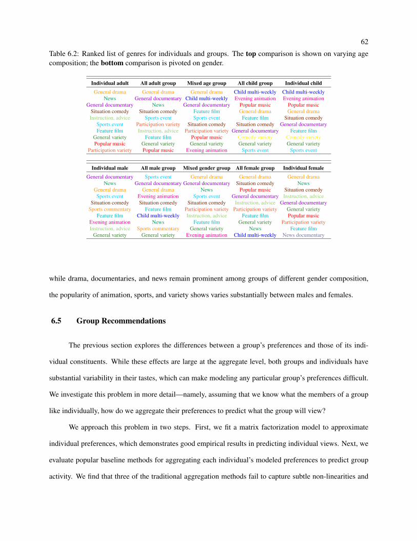
62
Table 6.2: Ranked list of genres for individuals and groups. The top comparison is shown on varying age
composition; the bottom comparison is pivoted on gender.
Individual adult All adult group Mixed age group All child group Individual child
General drama General drama General drama Child multi-weekly Child multi-weekly
News General documentary Child multi-weekly Evening animation Evening animation
General documentary News General documentary Popular music Popular music
Situation comedy Situation comedy Feature film General drama General drama
Instruction, advice Sports event Sports event Feature film Situation comedy
Sports event Participation variety Situation comedy Situation comedy General documentary
Feature film Instruction, advice Participation variety General documentary Feature film
General variety Feature film Popular music Comedy variety Comedy variety
Popular music General variety General variety General variety General variety
Participation variety Popular music Evening animation Sports event Sports event
Individual male All male group Mixed gender group All female group Individual female
General documentary Sports event General drama General drama General drama
News General documentary General documentary Situation comedy News
General drama General drama News Popular music Situation comedy
Sports event Evening animation Sports event General documentary Instruction, advice
Situation comedy Situation comedy Situation comedy Instruction, advice General documentary
Sports commentary Feature film Participation variety Participation variety General variety
Feature film Child multi-weekly Instruction, advice Feature film Popular music
Evening animation News Feature film General variety Participation variety
Instruction, advice Sports commentary General variety News Feature film
General variety General variety Evening animation Child multi-weekly News documentary
while drama, documentaries, and news remain prominent among groups of different gender composition,
the popularity of animation, sports, and variety shows varies substantially between males and females.
6.5 Group Recommendations
The previous section explores the differences between a group’s preferences and those of its indi-
vidual constituents. While these effects are large at the aggregate level, both groups and individuals have
substantial variability in their tastes, which can make modeling any particular group’s preferences difficult.
We investigate this problem in more detail—namely, assuming that we know what the members of a group
like individually, how do we aggregate their preferences to predict what the group will view?
We approach this problem in two steps. First, we fit a matrix factorization model to approximate
individual preferences, which demonstrates good empirical results in predicting individual views. Next, we
evaluate popular baseline methods for aggregating each individual’s modeled preferences to predict group
activity. We find that three of the traditional aggregation methods fail to capture subtle non-linearities and

63
interactions between individual preferences, which we are able to estimate directly from our large-scale
dataset. We propose a relatively simple model to account for these features that provides further insight into
group decision making.
6.5.1 Modeling Individuals
To examine how to best combine preferences of individuals in a group, we first need a means of deter-
mining each individual user’s interest in each telecast in our dataset. We use the Matchbox recommendation
system [86] without features, which fits a matrix factorization model to user’s individual viewing activity to
approximate these preferences.
Fitting such a model requires information about both “positive examples”—the telecasts that a given
individual viewed—and “negative examples”—telecasts that were available to individuals but not consumed.
Unfortunately our dataset lacks negative examples, so we approximate this set as follows: for each telecast
viewed by an individual, we consider all simultaneously broadcast telecasts on all channels in a user’s view-
ing history as potential negative examples. This results in roughly 16 negative examples for every positive
example across the dataset. To keep a balanced number of positive and negative examples in our training
set, we sample one negative example for each positive one, weighting telecasts by overall popularity [71].
We train Matchbox using this dataset with K = 20 latent trait dimensions on a randomly selected
training set composed of 80% of the individual view data set, with the remaining 20% of individual views
used for the test set. We set the user threshold prior and noise variances to 0, assuming a time-invariant
threshold and a binary likelihood function. We place flexible priors on users and items by setting the user
trait variance and item trait variance hyperparameters to 1√K
, and the user bias variance and item bias
variance hyperparameters to 1. The best-fit individual model found by Matchbox has an AUC of 88.3%
on the held-out test set. Given this performance, we consider the model to be a reliable approximation to
individual preferences and next investigate the group recommendation problem.
64
6.5.2 Preference Aggregation
As noted in our overview of related work, there are many approaches to aggregating individual pref-
erences. Here we investigate three of the simplest, which are commonly used: least misery, average satis-
faction, and maximum satisfaction. Denoting individual preference that user u has for item i by pui, these
methods predict group preferences as follows:
least misery : minu∈Gpui
average satisfaction : 1|G|
∑
u∈G pui
max satisfaction : maxu∈Gpui.
Least misery aims to minimize dissatisfaction of the least satisfied individual, maximum satisfaction to
maximize enjoyment of the most satisfied, and average satisfaction takes an equal vote amongst all members.
After learning individual preferences with Matchbox, we evaluate each of these aggregation methods
on all group views in our dataset. We find a strict ordering in terms of performance, with maximum satis-
faction slightly outperforming average satisfaction, and both dominating least misery, across and within all
group types. We find an overall AUC of 83.0% for maximum satisfaction, 82.6% for average satisfaction,
and 79.7% for least misery. In further examining the quality of group predictions by group type, we see that
mixed age and mixed gender group views are the most difficult to predict, with an AUC of 81.3%. Like-
wise, groups of all children are easiest to model, with performance on all male groups being considerably
higher compared to all female groups (AUCs of 89.7% and 84.1%, respectively). Note that these results
are obtained with maximum satisfaction and are largely consistent with the individual-to-group similarity
comparison in Figure 6.5.
While some work on preference aggregation has been constrained to these relatively simple functions
over individual preferences, our large-scale dataset of hundreds of thousands of group views enables us
to conduct a direct examination of group preference landscapes. For simplicity, we limit this analysis to
groups of only two members (which comprise 80% of all group views). For each group viewing event in our
dataset, we bin the individual predicted probability for each member of the group to the nearest ten percent
and aggregate views to examine the empirical probability of a group view within each bin. Panel 3 of

65
0.00.2 0.4 0.6 0.8 1.0
0.00.2
0.40.6
0.81.00.0
0.2
0.4
0.6
0.8
1.0
Female
Male
Gro
up
Average
0.00.2 0.4 0.6 0.8 1.0
0.00.2
0.40.6
0.81.00.0
0.2
0.4
0.6
0.8
1.0
Female
Male
Gro
up
Max
0.00.2 0.4 0.6 0.8 1.0
0.00.2
0.40.6
0.81.00.0
0.2
0.4
0.6
0.8
1.0
Female
Male
Gro
up
Empirical
0.00.2 0.4 0.6 0.8 1.0
0.00.2
0.40.6
0.81.00.0
0.2
0.4
0.6
0.8
1.0
Female
Male
Gro
up
Modeled
Figure 6.8: Modeled and actual probability of group viewing as a function of individual viewing for 2-
person, mixed-gender adult couples.
Figure 6.8 shows the result for adult mixed gender couples, with the binned male’s and female’s preference
on the x- and y-axis, respectively, and the probability of a group view on the z-axis. The predicted landscape
for average satisfaction and maximum satisfaction are shown in the first two panels for comparison, from
which it is clear that these traditional aggregation functions are overly simple, missing crucial interactions
and non-linearities in the group preference landscape.
The empirical landscape appears to be a mixture of the average and maximum satisfaction functions,
but differs from both of these functions along the diagonal, where users share identical individual prefer-
ences. For example, when both individuals equally dislike a program, there is a lower probability that the
group will view the show than traditional approaches suggest. This difference is highlighted in Figure 6.9a,
where the dotted line indicates the (identical) predictions made by average satisfaction, least misery, and
maximum satisfaction, whereas the points show the empirical probabilities of group viewing. We see a sim-
ilar deviation when matched preferences are large, showing a slightly higher likelihood of group viewing
than naive methods predict. We also see that average satisfaction deals poorly with the extremes: for exam-
ple, when one individual has a strong preference for a show while the other has a strong preference against
it. One explanation for this behavior is a repeated bargaining scenario where groups alternate between
satisfying a different individual in each instance.
In addition to differing from the three simple aggregation functions discussed above, the empirical
landscape also deviates from predictions made by other popular aggregation methods [64]. For instance,
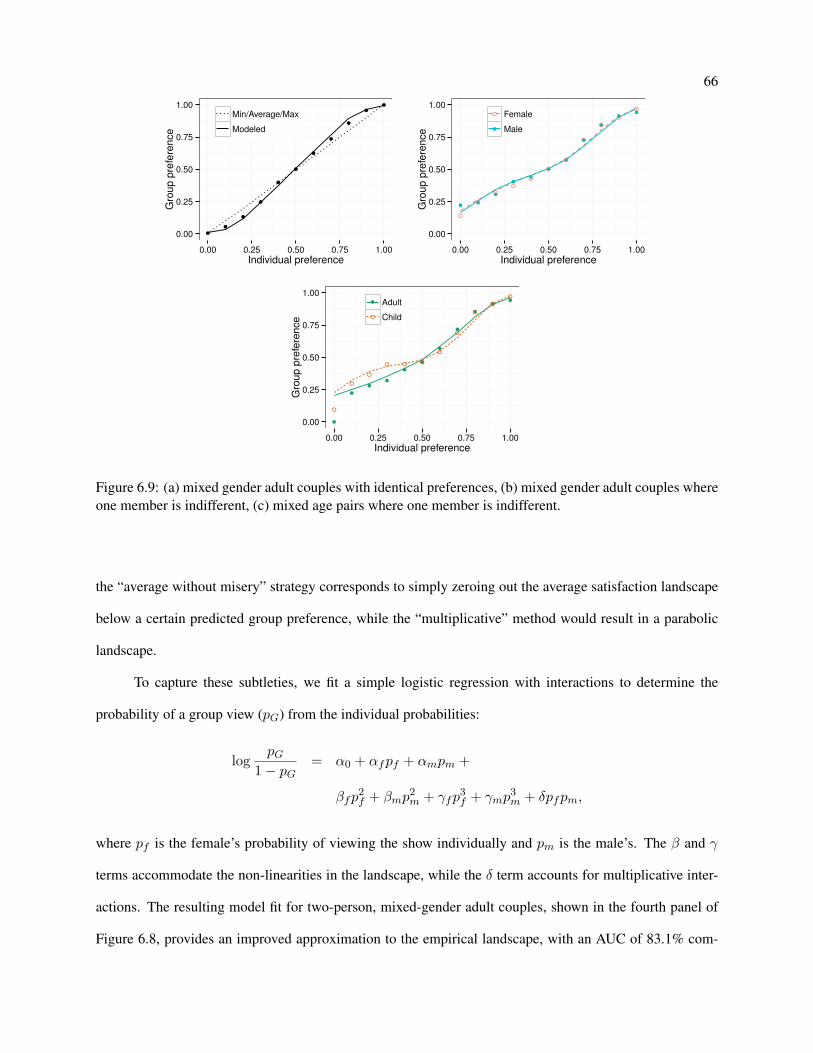
66
●
●
●
●
●
●
●
●
●
●
●0.00
0.25
0.50
0.75
1.00
0.00 0.25 0.50 0.75 1.00
Individual preference
Gro
up p
refe
rence
Min/Average/Max
Modeled●
●
●
●
●
●
●
●
●
●●
●
●
●
●
●
●
●
●
●
●
●
0.00
0.25
0.50
0.75
1.00
0.00 0.25 0.50 0.75 1.00
Individual preference
Gro
up p
refe
rence
●
●
Female
Male
●
●
●
●
●
●
●
●
●
●
●
●
●
●
●
●
●
●
●
●
●
●
0.00
0.25
0.50
0.75
1.00
0.00 0.25 0.50 0.75 1.00
Individual preference
Gro
up p
refe
rence
●
●
Adult
Child
Figure 6.9: (a) mixed gender adult couples with identical preferences, (b) mixed gender adult couples where
one member is indifferent, (c) mixed age pairs where one member is indifferent.
the “average without misery” strategy corresponds to simply zeroing out the average satisfaction landscape
below a certain predicted group preference, while the “multiplicative” method would result in a parabolic
landscape.
To capture these subtleties, we fit a simple logistic regression with interactions to determine the
probability of a group view (pG) from the individual probabilities:
logpG
1− pG= α0 + αfpf + αmpm +
βfp2f + βmp2m + γfp
3f + γmp3m + δpfpm,
where pf is the female’s probability of viewing the show individually and pm is the male’s. The β and γ
terms accommodate the non-linearities in the landscape, while the δ term accounts for multiplicative inter-
actions. The resulting model fit for two-person, mixed-gender adult couples, shown in the fourth panel of
Figure 6.8, provides an improved approximation to the empirical landscape, with an AUC of 83.1% com-

67
pared to 82.9% and 82.7% for maximum satisfaction and average satisfaction, respectively, on a randomly
selected 20% held-out test set. Importantly, we note that while the differences in these aggregate metrics
may seem insignificant, the model performs substantially better in crucial portions of the landscape—for
example, traditional methods overpredict in regions where both group members dislike content (e.g., small
individual values in Figure 6.9a), leading to potential dissatisfaction and possibly lost of trust in the recom-
mender system. Aggregate metrics understate these improvements due to the non-uniform density of group
views along the landscape.
Figure 6.9b shows further details of the model for mixed-gender adult couples, taken along slices of
the landscape where either the male or female is indifferent, corresponding to a individual preference of
0.5. For instance, the blue curve in Figure 6.9b shows how the probability of a group view changes with the
male’s individual preference when the female’s preference is held fixed at 0.5, and vice versa for the pink
curve. This highlights two key observations: first, the modeled curves are far from (piecewise) linear, as
traditional aggregation functions would suggest, and second, we see no obvious signs of gender dominance.
We contrast this with Figure 6.9c, which shows the model fit for two-person mixed age groups. Here we
see an asymmetry between adults and children, where the marginal increase in a child’s interest at low
preference levels has higher impact than an adult’s.
We note that while we have discussed only mixed gender and age couples here, these same qual-
itative observations apply to other group types: a simple non-linear group model provides a better fit to
the empirical group landscape compared to traditional aggregation functions, which translates to improved
performance for group recommendations.
6.6 Summary
Throughout this study we have seen that groups are more complex than the sum of their parts. In
particular, we saw that viewing habits shift substantially between individual and group contexts, and groups
display markedly different preferences at the aggregate level depending on their demographic breakdowns.
This led to a detailed investigation of preference aggregation functions for modeling group decision mak-
ing. Owing to the unique nature of the large-scale observational dataset studied, we directly estimated

68
how individual preferences are combined in group settings, and observed subtle deviations from traditional
aggregation strategies.

Chapter 7
SocialDining: A Mobile Ad-hoc Group Recommendation Application
To demonstrate the feasibility of the individual and group-based recommender systems described in
Chapters 4 and 5 in a context-aware setting, we have developed a mobile ad-hoc group recommendation
application called SocialDining. SocialDining is targeted to individuals who want to meet with small groups
of friends, family, and acquaintances for food or drink at a local restaurant. SocialDining leverages the
individual and group-based recommender systems to recommend a number of restaurants that satisfies the
group members’ joint preferences. In this Chapter we describe typical use cases and the SocialDining user
interface in Section 7.1, provide some implementation details in Section 7.2, and present an initial analysis
of data collected from ongoing user studies in Section 7.3.
7.1 Use Cases
7.1.1 A host invites several friends to meet for lunch at an American Restaurant
In the following use case, we describe the actions that a user takes in inviting some friends to meet
for lunch at an American restaurant. We call this user the host.
(1) The host user begins on the main screen of the SocialDining mobile client, as shown in Figure 7.1.
On this screen, three tabs are apparent. The “Map” tab allows the host to browse nearby restaurants,
indicated by red place markers, and nearby friends, indicated by blue place markers (not shown).
The user’s current location is displayed as a small blue triangle (not shown). The user can tap
on a place marker to see more information about that restaurant or friend, as shown in the popup
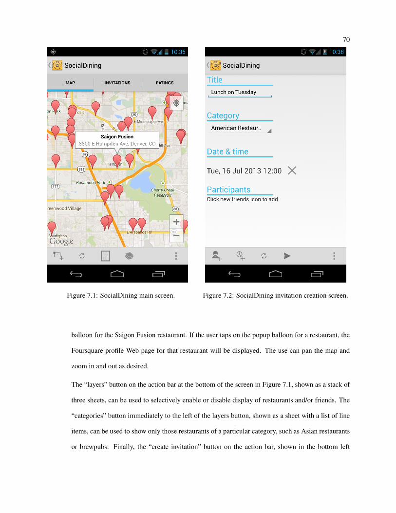
70
Figure 7.1: SocialDining main screen. Figure 7.2: SocialDining invitation creation screen.
balloon for the Saigon Fusion restaurant. If the user taps on the popup balloon for a restaurant, the
Foursquare profile Web page for that restaurant will be displayed. The use can pan the map and
zoom in and out as desired.
The “layers” button on the action bar at the bottom of the screen in Figure 7.1, shown as a stack of
three sheets, can be used to selectively enable or disable display of restaurants and/or friends. The
“categories” button immediately to the left of the layers button, shown as a sheet with a list of line
items, can be used to show only those restaurants of a particular category, such as Asian restaurants
or brewpubs. Finally, the “create invitation” button on the action bar, shown in the bottom left

71
corner of the screen, is used to create and send a new invitation. In this use case, the host user
proceeds to create a new invitation by tapping on the “create invitation” button.
(2) After tapping on the button to create a new invitation, the screen shown in Figure 7.2 appears. The
host can enter a title for the invitation, specify a restaurant category for the invitation, specify one
or more possible dates and times for the invitation, and specify one or more friends that should
be included as participants in the invitation. Finally, when the host is satisfied with the invitation
settings, the host taps the “send invitation” button, shown as a triangular symbol in the action bar
at the bottom of the screen, to send the invitation to all of the selected participants.
7.1.2 A user receives an invitation to meet several friends for lunch at an American Restaurant
In the following use case, we describe the actions that a user takes when he receives an invitation to
meet several friends for lunch at an American restaurant.
(1) First, the user receives a notification from the SocialDining application on his smartphone indicat-
ing that he has received a new invitation. The user responds to this notification and the SocialDining
application opens with the time voting screen displayed for this invitation, as shown in Figure 7.3.
The user can express his preferences for the date and time for the invitation by voting on one or
more possible options. The proposed dates and times specified by the host during invitation cre-
ation are displayed initially. In this use case, the user votes for 12:00 PM on July 16. Any user
may add a new proposed date and time to the list of options to vote for by tapping the “add time”
button, shown at the bottom of the screen as a clock with a plus sign. Once a user has added a
new proposed date and time, this new option is automatically made visible to all other invitation
participants for voting. Voting continues until the host finalizes the date and time for this invitation
by tapping the “finalize time” button, shown in the bottom left corner of the screen as a clock with
a check mark. Only the host is permitted to finalize the date and time for an invitation.
The user can open the “Participants” tab, shown in Figure 7.3, to view the list of participants for
this invitation. The user can remove himself from the participant list by tapping on the “x” button
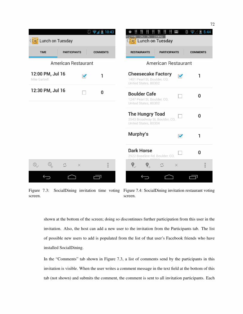
72
Figure 7.3: SocialDining invitation time voting
screen.
Figure 7.4: SocialDining invitation restaurant voting
screen.
shown at the bottom of the screen; doing so discontinues further participation from this user in the
invitation. Also, the host can add a new user to the invitation from the Participants tab. The list
of possible new users to add is populated from the list of that user’s Facebook friends who have
installed SocialDining.
In the “Comments” tab shown in Figure 7.3, a list of comments send by the participants in this
invitation is visible. When the user writes a comment message in the text field at the bottom of this
tab (not shown) and submits the comment, the comment is sent to all invitation participants. Each
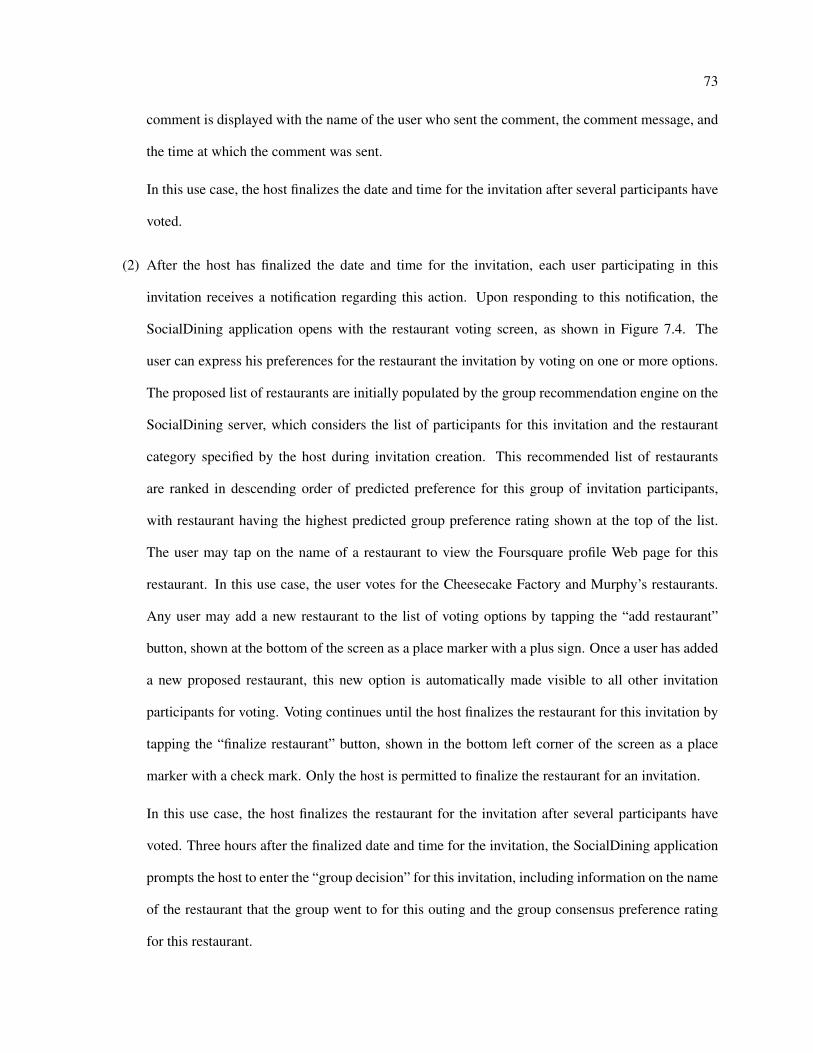
73
comment is displayed with the name of the user who sent the comment, the comment message, and
the time at which the comment was sent.
In this use case, the host finalizes the date and time for the invitation after several participants have
voted.
(2) After the host has finalized the date and time for the invitation, each user participating in this
invitation receives a notification regarding this action. Upon responding to this notification, the
SocialDining application opens with the restaurant voting screen, as shown in Figure 7.4. The
user can express his preferences for the restaurant the invitation by voting on one or more options.
The proposed list of restaurants are initially populated by the group recommendation engine on the
SocialDining server, which considers the list of participants for this invitation and the restaurant
category specified by the host during invitation creation. This recommended list of restaurants
are ranked in descending order of predicted preference for this group of invitation participants,
with restaurant having the highest predicted group preference rating shown at the top of the list.
The user may tap on the name of a restaurant to view the Foursquare profile Web page for this
restaurant. In this use case, the user votes for the Cheesecake Factory and Murphy’s restaurants.
Any user may add a new restaurant to the list of voting options by tapping the “add restaurant”
button, shown at the bottom of the screen as a place marker with a plus sign. Once a user has added
a new proposed restaurant, this new option is automatically made visible to all other invitation
participants for voting. Voting continues until the host finalizes the restaurant for this invitation by
tapping the “finalize restaurant” button, shown in the bottom left corner of the screen as a place
marker with a check mark. Only the host is permitted to finalize the restaurant for an invitation.
In this use case, the host finalizes the restaurant for the invitation after several participants have
voted. Three hours after the finalized date and time for the invitation, the SocialDining application
prompts the host to enter the “group decision” for this invitation, including information on the name
of the restaurant that the group went to for this outing and the group consensus preference rating
for this restaurant.
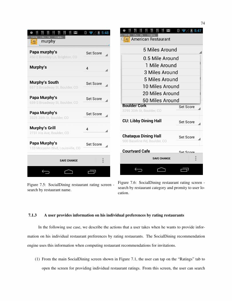
74
Figure 7.5: SocialDining restaurant rating screen -
search by restaurant name.
Figure 7.6: SocialDining restaurant rating screen -
search by restaurant category and promity to user lo-
cation.
7.1.3 A user provides information on his individual preferences by rating restaurants
In the following use case, we describe the actions that a user takes when he wants to provide infor-
mation on his individual restaurant preferences by rating restaurants. The SocialDining recommendation
engine uses this information when computing restaurant recommendations for invitations.
(1) From the main SocialDining screen shown in Figure 7.1, the user can tap on the “Ratings” tab to
open the screen for providing individual restaurant ratings. From this screen, the user can search
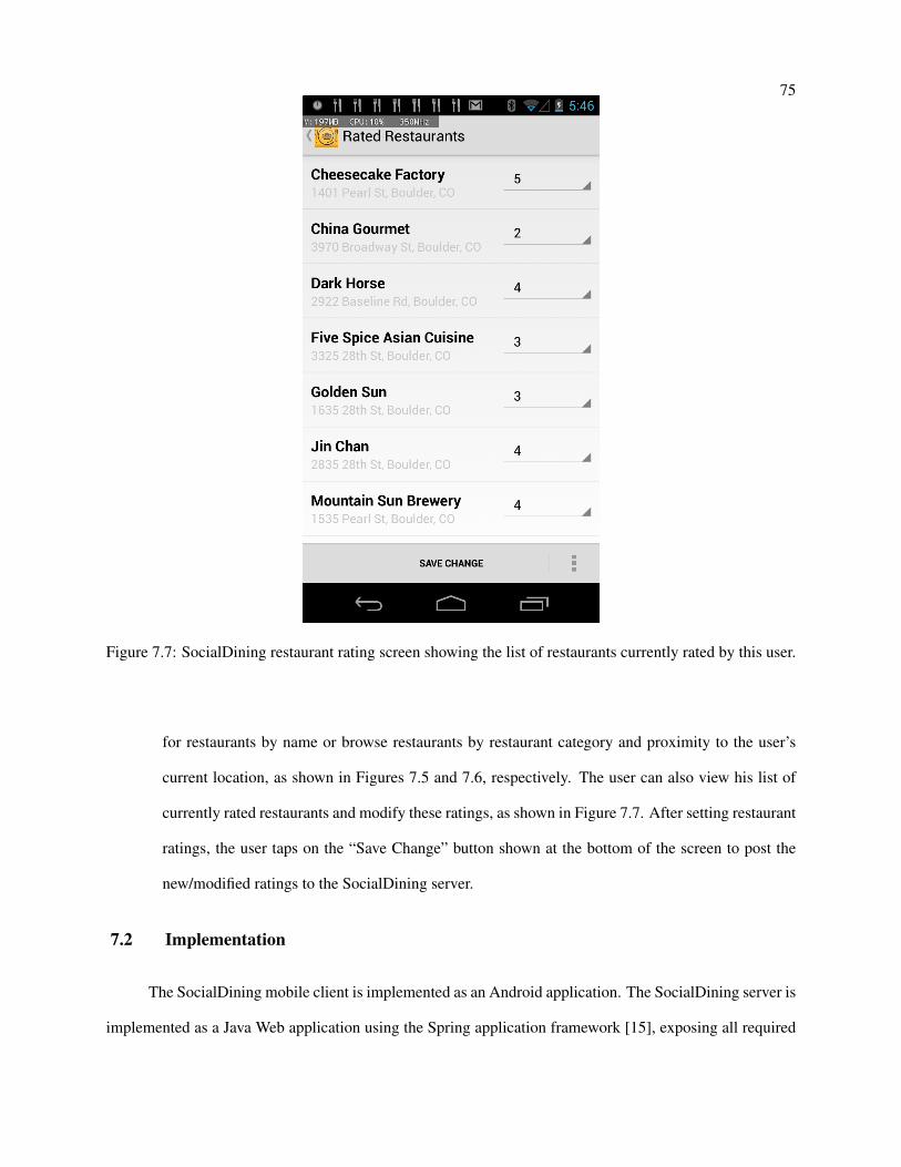
75
Figure 7.7: SocialDining restaurant rating screen showing the list of restaurants currently rated by this user.
for restaurants by name or browse restaurants by restaurant category and proximity to the user’s
current location, as shown in Figures 7.5 and 7.6, respectively. The user can also view his list of
currently rated restaurants and modify these ratings, as shown in Figure 7.7. After setting restaurant
ratings, the user taps on the “Save Change” button shown at the bottom of the screen to post the
new/modified ratings to the SocialDining server.
7.2 Implementation
The SocialDining mobile client is implemented as an Android application. The SocialDining server is
implemented as a Java Web application using the Spring application framework [15], exposing all required

76
functionality to the client through REST [36] APIs. MongoDB [10] is used to store and manage all data on
the server.
The SocialDining recommendation engine uses the individual and group-based recommender sys-
tems described in Chapters 4 and 5 to compute restaurant recommendations for each invitation, based on
the group of invitation participants and the specified restaurant category. Specifically, the Social Likelihood
model from Section 4.3.3 is used to compute recommendations for individuals, and the heuristic group con-
sensus function based on average satisfaction from Section 5.3.2 is used to compute recommendations for
groups. We chose to use the heuristic group consensus function based on average satisfaction since we did
not have a measure of social strength between each member of the groups in our user study, and therefore
assumed that most group members would share social connections of moderate strength. The information
about each restaurant in SocialDining is obtained from Foursquare. When launching the SocialDining ap-
plication for the first time after the application is installed, the user is prompted to log in using his Facebook
account. This Facebook account information is used to populate each SocialDining user account, including
the user’s name and Facebook friend list. This friend list is used to populate the social graph maintained
internally within SocialDining.
7.3 User Study
To investigate the quality of SocialDining recommendations and obtain user feedback on the Social-
Dining application, we conducted a user study for 15 weeks, from August – December 2012. We recruited
11 groups to participate in this study: eight groups of mutual friends and three romantic-couple groups. Each
group was composed of 2 – 5 individuals, with some individuals participating in two groups; a total of 31
individuals participated in this study. Each group participated in the study for a duration of 3 – 5 weeks. The
participants were undergraduate students, graduate students, and university staff. Data on approximately
500 restaurants in Boulder was obtained from Foursquare and used to populate the SocialDining restaurant
database, and participants were restricted to selecting from these restaurant when using SocialDining in this
study.

77
We describe some observations from the data collected during this user study in the next two sections.
In the following discussion, a “completed invitation” refers to an invitation where the host user for the invita-
tion has submitted information to SocialDining regarding the restaurant that the group went to for food/drink
for this invitation. Recall that the SocialDining application queries the host user for this information three
hours after the finalized event date and time for an invitation has passed; this information submitted by the
host for an invitation is referred to as a “group decision” below.
7.3.1 SocialDining Restaurant Recommendations
Table 7.1 shows historical data for the invitations completed over the course of our user study, in-
cluding the number of invitations completed, the number of invitations where the group decision matches a
recommended restaurant, and the number of invitations where the group decision matches a restaurant that
has been added to the invitation by one of the invitation participants. This data shows that the group deci-
sion matches a restaurant recommendation provided by SocialDining for approximately 50% of completed
invitations. Of the remaining 50% of completed invitations, the group decision matches a restaurant added
to the invitation by a participant about 70% of the time. Therefore, for about 15% of completed invitations,
users appear to use a communication channel that does not involve explicit voting on restaurants in the So-
cialDining app when determining the group decision. This channel may involve comments within the app,
or some other mechanism such as SMS text messages, email, etc.
In Table 7.1 we define “display rank” as the position in the ranked list of SocialDining restaurant
recommendations where the group-decision restaurant is found, for an invitation where the group decision
matches one of the recommendations. Therefore, we see from this table that for those invitations where the
group decision matches a recommendation, the group decision is generally found near the third most highly
ranked recommendation, which suggests that the SocialDining recommendation engine performs reasonably
well in surfacing relevant recommendations.
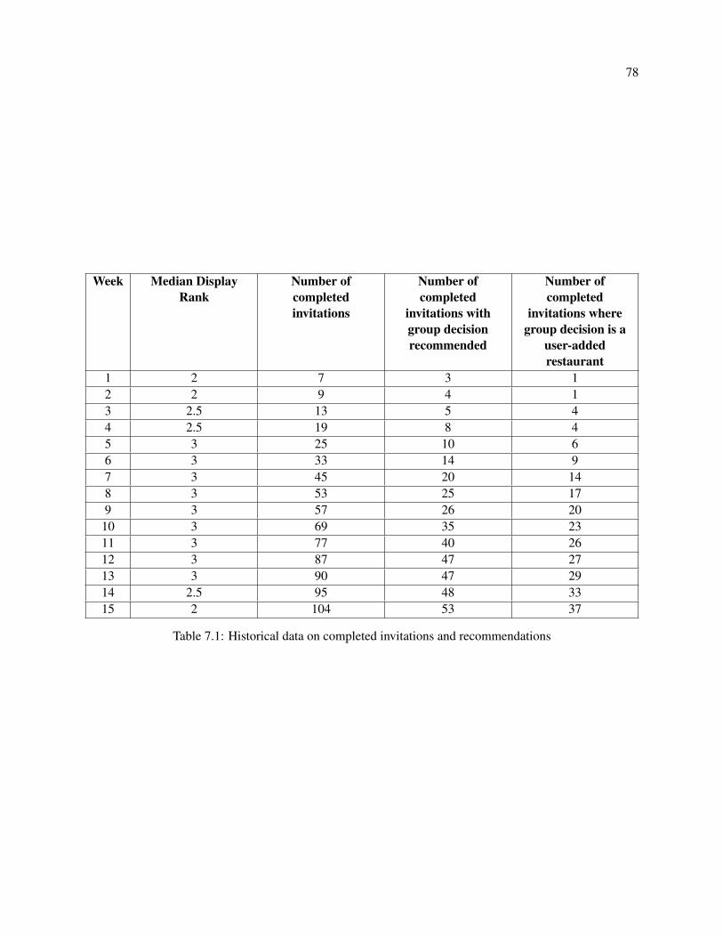
78
Week Median Display
Rank
Number of
completed
invitations
Number of
completed
invitations with
group decision
recommended
Number of
completed
invitations where
group decision is a
user-added
restaurant
1 2 7 3 1
2 2 9 4 1
3 2.5 13 5 4
4 2.5 19 8 4
5 3 25 10 6
6 3 33 14 9
7 3 45 20 14
8 3 53 25 17
9 3 57 26 20
10 3 69 35 23
11 3 77 40 26
12 3 87 47 27
13 3 90 47 29
14 2.5 95 48 33
15 2 104 53 37
Table 7.1: Historical data on completed invitations and recommendations

79Number of invitations Median distance in km between closest user
location cluster and group-decision restaurant
37 1.857
Table 7.2: Location impact on invitations where the group decision matches a recommendation
7.3.2 Location Impact on Group Decisions
The SocialDining client application posts the user’s current location to the server every five minutes,
if the application is running in the background, or every 30 seconds, if the app is running in the foreground.
The user may disable location tracking at any time in the application, which prevents the application from
posting location data to the server.
To investigate the impact of user location on group decision behavior in SocialDining, we examine
a subset of the data captured during our user study from weeks 1 – 13. First, we apply the DBSCAN
clustering algorithm [35] to find spatial clusters in the temporally-ordered location trace data for each user
who participated in our study. The DBSCAN ǫ parameter is set to 1.0 km, and the parameter for the
minimum number of points required to form a dense region is set to 40. We found that these DBSCAN
parameter settings find sensible clusters in our location trace based on a visual inspection of these clusters
plotted on a map, and these clusters appear to correspond to locations frequented by our study participants,
such as work, school, home, etc. Next, for each completed invitation, and for each invitation participant,
we identify the participant user location cluster that is closest to the group decision restaurant for that
invitation, with the requirement that this cluster must contain a point with a timestamp that occurs within
two hours before or after the finalized event date and time for the invitation. Table 7.2 shows the median
distance between the closest invitation participant location cluster and the group decision restaurant for
those initiations where the group decision matches one of the recommendations provided by SocialDining,
and Table 7.3 shows the median distance for those invitations where the group decision does not match a
recommendation. Note that some invitations were omitted, due to lack of user location clusters satisfying the
requirements described above. We see from these tables that the median distance between the closest user
location cluster and group decision restaurant is approximately 42% smaller for those invitations where the

80Number of invitations Median distance in km between closest user
location cluster and group-decision restaurant
31 1.074
Table 7.3: Location impact on invitations where the group decision does not match a recommendation
group decision does not match a recommendation. Therefore, we infer that for those invitations where the
invitation participants do not elect one of the recommendations, restaurant proximity to the user’s location
may be an important factor. For example, we would intuitively expect that users would prefer to go to lunch
at restaurants that are close to their place of work or school at certain times, such as a weekday afternoon.
7.4 Summary
In this chapter we have proposed a mobile ad-hoc group recommendation application called Social-
Dining. SocialDining leverages the individual and group-based recommender systems described in Chap-
ters 4 and 5, respectively, to compute restaurant recommendations for small groups of users who plan to
dine or drink at the restaurant together. We have described the functionality and user interface provided by
SocialDining, discussed some implementation details, and presented a preliminary analysis of data collected
from our user studies. We see that SocialDining generally provides relevant recommendations for approx-
imately 50% of the invitations completed by our study participants. For those invitations where the group
does not decide to go to one of the recommended restaurants, restaurant proximity to one or more invitation
participants appears to be a significant factor.
Chapter 8
Conclusions
This thesis has presented, implemented, and evaluated new approaches to recommender systems for
individuals and groups of individuals that leverage social indicators in novel ways. These approaches are
designed to improve the predictive quality of recommender systems for individuals and small groups. Since
online social networks (OSNs), such as Facebook, have become quite pervasive, this work leverages social
networks as the primary source of social indicators. The recommender systems proposed in this work were
evaluated using small-scale datasets obtained from offline experiments, and large-scale datasets obtained
from OSNs and from household TV viewing data collected by Nielsen. Significant research challenges
were involved in the algorithmic design, implementation, and evaluation of these recommender systems.
To demonstrate the feasibility of the the individual and group-based recommender systems described in
Chapters 4 and 5, respectively, we implemented the SocialDining mobile application and conducted a user
study involving this application. SocialDining provides restaurant recommendations for small groups of
users who plan to dine or drink at a restaurant together. We conducted an analysis of some of the data
obtained from this user study, revealing insights regarding recommendation quality and preference behavior
in SocialDining.
8.1 Summary
In Chapter 4 we proposed and investigated two novel models for including a social network in a
Bayesian framework for recommendation using matrix factorization. The first model, which we call the
Edge MRF model, places the social network in the prior distribution over user features as a Markov Random

82
Field that describes user similarity. The second model, called the Social Likelihood model, treats social links
as observations and places the social network in the likelihood function. We evaluated both models using a
large scale dataset collected from the Flixster online social network. Experimental results indicate that while
both models perform well, the Social Likelihood model outperforms existing methods for recommendation
in social networks when considering cold start users who have rated few items.
We developed a novel group recommendation solution that incorporates both social and content in-
terests of group members in Chapter 5. We studied several key group characteristics that impact group deci-
sions, and proposed a group consensus function that captures the social, expertise, and interest dissimilarity
among group members. Furthermore, we described a generic framework that can automatically analyze
various group characteristics and generate the corresponding group consensus function. Both the consensus
function we developed and the generic framework perform well on real-world user studies consisting of
groups of various sizes, user interests, and social relationships.
Throughout the large-scale study presented in Chapter 6 we saw that groups are more complex than
the sum of their parts. In particular, we saw that viewing habits shift substantially between individual
and group contexts, and groups display markedly different preferences at the aggregate level depending
on their demographic breakdowns. This led to a detailed investigation of preference aggregation functions
for modeling group decision making. Owing to the unique nature of the large-scale observational dataset
studied, we directly estimated how individual preferences are combined in group settings, and observed
subtle deviations from traditional aggregation strategies.
Chapter 7 proposed a mobile ad-hoc group recommendation application called SocialDining. So-
cialDining leverages the individual and group-based recommender systems described in Chapters 4 and 5,
respectively, to compute restaurant recommendations for small groups of users who plan to dine or drink at
a restaurant together. We described the functionality and user interface provided by SocialDining, discussed
some implementation details, and presented a preliminary analysis of data collected from our user studies.
We see that SocialDining generally provides relevant recommendations for approximately 50% of the invi-
tations completed by our study participants. For those invitations where the group does not decide to go to

83
one of the recommended restaurants, restaurant proximity to one or more invitation participants appears to
be a significant factor.
8.2 Future Work
The work presented in Chapter 4 suggests several interesting directions for future work. The Social
Likelihood model described in this chapter requires that the s parameter, which controls the influence of the
social network, be set manually. We believe that this model could be enhanced to automatically learn the
optimal value of s during training, possibly using a Metropolis-Hastings sampling step [47], which would
allow us to sample for s using a proposal density that is proportional to the density of s. Additionally,
we would like to investigate approaches to decreasing the execution time of the sampler implemented for
the Social Likelihood model. While we can easily speed up sampling for items by sampling from the
conditional distributions for items in parallel, parallel sampling for users cannot be trivially implemented,
since the conditional distribution for a user is dependent on its neighbors, as shown in Equation 4.16.
While we were able to explain observed group behavior in Chapter 6 with a relatively simple model,
these results raise a number of questions. For example, further investigation is required to understand why
these preference landscapes take the shape they do, with third-order non-linearities. Likewise, untangling the
driving forces behind these observations requires more than simple observational data. On one hand, effects
could be explained by direct influence of individuals on each other, while on the other hand these outcomes
may be confounded with homophily, wherein individuals tend to preferentially participate in groups that
share their tastes. We leave answers to these questions along with generalizations to arbitrary group settings
as future work.
The work presented in Chapter 6 indicates that group context is important when modeling group
preference behavior. This work identified a number of explicit group contexts that impact group preferences,
such as groups composed of a mix of members of varying ages and genders. We believe that group context
could be seen as inhabiting a latent trait space, similar to how users inhabit a latent user trait space in
the matrix factorization framework for individual recommendation. We leave the development of a fully
probabilistic model for group recommendation that incorporates this idea as future work.

84
The SocialDining user study presented in Section 7.3 was conducted at a relatively small scale, with
32 individual participants and 104 completed invitations. We would like to conduct a SocialDining study
at larger scale, involving on the order of hundreds participants and thousands of completed invitations.
The data collected from such a study would allow us to further investigate individual and group preference
behavior in this domain, particularly regarding how location and other contextual factors impact preferences.
Additionally, a larger dataset would facilitate the development and evaluation of a probabilistic model for
group recommendation customized for this application. Plans are currently underway to conduct such a
large-scale SocialDining study.
Bibliography
[1] Amazon. http://www.amazon.com.
[2] Facebook. http://www.facebook.com.
[3] The facebook blog - our first 100 million. http://blog.facebook.com/blog.php?post=
28111272130.
[4] Facebook now has more than a billion mobile users every month. http://www.theverge.com/
2014/4/23/5644740/facebook-q1-2014-earnings.
[5] Flixster data set. http://www.cs.sfu.ca/˜sja25/personal/datasets/.
[6] Google+. http://plus.google.com.
[7] Google news. http://news.google.com.
[8] IMDB. http://www.imdb.com.
[9] Linkedin. http://www.linkedin.com.
[10] Mongodb. http://www.mongodb.org/.
[11] Movielens data sets. http://www.grouplens.org/node/73.
[12] The music genome project. http://www.pandora.com/mgp.shtml.
[13] Netflix. http://www.netflix.com.
[14] Pandora. http://www.pandora.com.
[15] Spring framework. http://projects.spring.io/spring-framework/.
[16] Gediminas Adomavicius and Alexander Tuzhilin. Toward the next generation of recommender sys-
tems: A survey of the state-of-the-art and possible extensions. IEEE Transactions on Knowledge and
Data Engineering, 17:734–749, 2005.
[17] R. Agrawal, T. Imielinski, and A. Swami. Mining association rules between sets of items in large
databases. In Proc. of SIGMOD 1993, pages 207–216, 1993.
[18] R. Agrawal and R. Srikant. Fast algorithms for mining association rules. In Proc. of VLDB 1994,
volume 1215, pages 487–499, 1994.

86
[19] Sihem Amer-Yahia, Senjuti Basu Roy, Ashish Chawla, Gautam Das, and Cong Yu. Group recommen-
dation: Semantics and efficiency. In Proc. of VLDB 2009.
[20] M. Baldauf, S. Dustdar, and F. Rosenberg. A survey on context-aware systems. International Journal
of Ad Hoc and Ubiquitous Computing, 2(4):263–277, 2007.
[21] Linas Baltrunas, Tadas Makcinskas, and Francesco Ricci. Group recommendations with rank aggre-
gation and collaborative filtering. In Proceedings of the fourth ACM conference on Recommender
systems, RecSys ’10, pages 119–126, New York, NY, USA, 2010. ACM.
[22] A. Beach, M. Gartrell, S. Akkala, J. Elston, J. Kelley, K. Nishimoto, B. Ray, S. Razgulin, K. Sundare-
san, B. Surendar, et al. Whozthat? evolving an ecosystem for context-aware mobile social networks.
Network, IEEE, 22(4):50–55, 2008.
[23] A. Beach, M. Gartrell, X. Xing, R. Han, Q. Lv, S. Mishra, and K. Seada. Fusing mobile, sensor, and
social data to fully enable context-aware computing. In Proc. of HotMobile 2010, pages 60–65, 2010.
[24] Shlomo Berkovsky, Jill Freyne, and Mac Coombe. Aggregation trade offs in family based recommen-
dations. In Proc. of the 22nd Australasian Joint Conference on Advances in Artificial Intelligence,
2009.
[25] Claudio Biancalana, Fabio Gasparetti, Alessandro Micarelli, Alfonso Miola, and Giuseppe San-
sonetti. Context-aware movie recommendation based on signal processing and machine learning. In
Proceedings of the 2nd Challenge on Context-Aware Movie Recommendation, CAMRa ’11, pages
5–10, New York, NY, USA, 2011. ACM.
[26] G. Biegel and V. Cahill. A framework for developing mobile, context-aware applications.
In Proceedings of the Second IEEE International Conference on Pervasive Computing and
Communications (PerCom’04), page 361, 2004.
[27] Ludovico Boratto, Salvatore Carta, Alessandro Chessa, Maurizio Agelli, and M. Laura Clemente.
Group recommendation with automatic identification of users communities. In Proc. of WI-IAT ’09,
2009.
[28] J.S. Breese, D. Heckerman, C. Kadie, et al. Empirical analysis of predictive algorithms for collabo-
rative filtering. In Proceedings of the 14th conference on Uncertainty in Artificial Intelligence, pages
43–52, 1998.
[29] Allison JB Chaney, Mike Gartrell, Jake M Hofman, John Guiver, Noam Koenigstein, Pushmeet Kohli,
and Ulrich Paquet. A large-scale exploration of group viewing patterns. In Proceedings of the 1st
ACM international conference on interactive experiences for television and online video, TVX 2014.
ACM, 2014. To appear.
[30] Abhinandan S. Das, Mayur Datar, Ashutosh Garg, and Shyam Rajaram. Google news personalization:
Scalable online collaborative filtering. In Proc. of WWW ’07, pages 271–280, 2007.
[31] L.M. de Campos, J.M. Fernandez-Luna, J.F. Huete, and M.A. Rueda-Morales. Managing uncertainty
in group recommending processes. Journal of User Modeling and User-Adapted Interaction, 19, 2009.
[32] M. Deshpande and G. Karypis. Item-based top-n recommendation algorithms. ACM Transactions on
Information Systems (TOIS), 22(1):143–177, 2004.

87
[33] A.K. Dey, G.D. Abowd, and D. Salber. A conceptual framework and a toolkit for supporting the rapid
prototyping of context-aware applications. Human-Computer Interaction, 16(2):97–166, 2001.
[34] W. K. Edwards and R. Grinter. At home with ubiquitous computing: Seven challenges. In Proceedings
of the 3rd International Conference on Ubiquitous Computing (Ubicomp 2001), pages 256–272, May
2001.
[35] Martin Ester, Hans-Peter Kriegel, Jorg Sander, and Xiaowei Xu. A density-based algorithm for dis-
covering clusters in large spatial databases with noise. In KDD, volume 96, pages 226–231, 1996.
[36] Roy T Fielding and Richard N Taylor. Principled design of the modern web architecture. ACM
Transactions on Internet Technology (TOIT), 2(2):115–150, 2002.
[37] Mike Gartrell, Ulrich Paquet, and Ralf Herbrich. A bayesian treatment of social links in recommender
systems. CU Technical Report CU-CS-1092-12, 2012.
[38] Mike Gartrell, Xinyu Xing, Qin Lv, Aaron Beach, Richard Han, Shivakant Mishra, and Karim Seada.
Enhancing group recommendation by incorporating social relationship interactions. In Proceedings of
the 16th ACM international conference on Supporting group work, GROUP ’10, pages 97–106, New
York, NY, USA, 2010. ACM.
[39] S. Geman and D. Geman. Stochastic relaxation, gibbs distributions, and the bayesian restoration of
images. Pattern Analysis and Machine Intelligence, IEEE Transactions on, (6):721–741, 1984.
[40] Gwangseop Gim, Hogyeong Jeong, Hyunjong Lee, and Dohyun Yun. Group-aware prediction with ex-
ponential smoothing for collaborative filtering. In Proceedings of the 2nd Challenge on Context-Aware
Movie Recommendation, CAMRa ’11, pages 11–14, New York, NY, USA, 2011. ACM.
[41] J Golbeck. Computing and Applying Trust in Web-based Social Networks. PhD thesis, University of
Maryland College Park, 2005.
[42] Gerald Joseph Goodhardt, Andrew Samuel Christopher Ehrenberg, Martin Alan Collins, et al. The
television audience: patterns of viewing. An update. Number Ed. 2. Gower Publishing Co. Ltd., 1987.
[43] Jagadeesh Gorla, Neal Lathia, Stephen Robertson, and Jun Wang. Probabilistic group recommendation
via information matching. In Proceedings of the 22nd international conference on World Wide Web,
WWW ’13, pages 495–504, Republic and Canton of Geneva, Switzerland, 2013. International World
Wide Web Conferences Steering Committee.
[44] Hansu Gu, Mike Gartrell, Liang Zhang, Qin Lv, and Dirk Grunwald. Anchormf: towards effective
event context identification. In Proceedings of the 22nd ACM international conference on information
& knowledge management, CIKM 2013, pages 629–638. ACM, 2013.
[45] T. Gu, H.K. Pung, and D.Q. Zhang. A service-oriented middleware for building context-aware services.
Journal of Network and Computer Applications, 28(1):1–18, 2005.
[46] J. Han, J. Pei, Y. Yin, and R. Mao. Mining frequent patterns without candidate generation: A frequent-
pattern tree approach. Data mining and knowledge discovery, 8(1):53–87, 2004.
[47] W Keith Hastings. Monte carlo sampling methods using markov chains and their applications.
Biometrika, 57(1):97–109, 1970.

88
[48] Xun Hu, Xiangwu Meng, and Licai Wang. Svd-based group recommendation approaches: an ex-
perimental study of moviepilot. In Proceedings of the 2nd Challenge on Context-Aware Movie
Recommendation, CAMRa ’11, pages 23–28, New York, NY, USA, 2011. ACM.
[49] Mohsen Jamali and Martin Ester. Trustwalker: a random walk model for combining trust-based and
item-based recommendation. In Proceedings of the 15th ACM SIGKDD international conference on
Knowledge discovery and data mining, KDD ’09, pages 397–406, New York, NY, USA, 2009. ACM.
[50] Mohsen Jamali and Martin Ester. A matrix factorization technique with trust propagation for rec-
ommendation in social networks. In Proceedings of the fourth ACM conference on Recommender
systems, RecSys 2010, pages 135–142, New York, NY, USA, 2010. ACM.
[51] Anthony Jameson and Barry Smyth. Recommendation to groups. In The adaptive web: methods and
strategies of web personalization, 2007.
[52] R. Jin, J.Y. Chai, and L. Si. An automatic weighting scheme for collaborative filtering. In Proceedings
of the 27th annual international ACM SIGIR conference on Research and development in information
retrieval, pages 337–344. ACM, 2004.
[53] Heung-Nam Kim, Majdi Rawashdeh, and Abdulmotaleb El Saddik. Tailoring recommendations to
groups of users: a graph walk-based approach. In Proceedings of the 2013 international conference on
Intelligent user interfaces, IUI ’13, pages 15–24, New York, NY, USA, 2013. ACM.
[54] Y. Koren, R. Bell, and C. Volinsky. Matrix factorization techniques for recommender systems.
Computer, 42(8):30–37, 2009.
[55] Yehuda Koren. The bellkor solution to the netflix grand prize. http://www.netflixprize.
com/assets/GrandPrize2009_BPC_BellKor.pdf, 2009.
[56] W. Li, J. Han, and J. Pei. Cmar: accurate and efficient classification based on multiple class-association
rules. In Proc. of ICDM 2001, pages 369–376, 2001.
[57] G. Linden, B. Smith, and J. York. Amazon. com recommendations: Item-to-item collaborative filtering.
Internet Computing, IEEE, 7(1):76–80, 2003.
[58] Greg Linden, Brent Smith, and Jeremy York. Amazon.com recommendations: Item-to-item collabo-
rative filtering. IEEE Internet Computing, 7:76–80, 2003.
[59] B. Liu, W. Hsu, and Y. Ma. Integrating classification and association rule mining. Proc. of KDD 1998,
pages 80–86, 1998.
[60] Hao Ma, Irwin King, and Michael R. Lyu. Learning to recommend with social trust ensemble.
In Proceedings of the 32nd international ACM SIGIR conference on Research and development in
information retrieval, SIGIR 2009, pages 203–210, New York, NY, USA, 2009. ACM.
[61] Hao Ma, Haixuan Yang, Michael R. Lyu, and Irwin King. Sorec: social recommendation using proba-
bilistic matrix factorization. In Proceeding of the 17th ACM conference on Information and knowledge
management, CIKM 2008, pages 931–940, New York, NY, USA, 2008. ACM.
[62] Hao Ma, Dengyong Zhou, Chao Liu, Michael R. Lyu, and Irwin King. Recommender systems with
social regularization. In Proceedings of the fourth ACM international conference on Web search and
data mining, WSDM 2011, pages 287–296, New York, NY, USA, 2011. ACM.
89
[63] Paolo Massa and Paolo Avesani. Trust-aware recommender systems. In Proceedings of the 2007 ACM
conference on Recommender systems, RecSys ’07, pages 17–24, New York, NY, USA, 2007. ACM.
[64] Judith Masthoff. Group modeling: Selecting a sequence of television items to suit a group of viewers.
Journal of User Modeling and User-Adapted Interaction, 14(1), 2004.
[65] John A McCarty and LJ Shrum. The role of personal values and demographics in predicting television
viewing behavior: Implications for theory and application. Journal of Advertising, 22(4):77–101,
1993.
[66] Emiliano Miluzzo, Nicholas D. Lane, Kristof Fodor, Ronald Peterson, Hong Lu, Mirco Musolesi,
Shane B. Eisenman, Xiao Zheng, and Andrew T. Campbell. Sensing meets mobile social networks:
the design, implementation and evaluation of the cenceme application. In Proc. of the 6th ACM Conf.
on Embedded Network Sensor Systems (SenSys 2008). ACM, Nov. 2008.
[67] Andres Moreno, Harold Castro, and Michel Riveill. Simple time-aware and social-aware user simi-
larity for a knn-based recommender system. In Proceedings of the 2nd Challenge on Context-Aware
Movie Recommendation, CAMRa ’11, pages 36–38, New York, NY, USA, 2011. ACM.
[68] Eirini Ntoutsi, Kostas Stefanidis, Kjetil Nørvag, and Hans-Peter Kriegel. Fast group recommendations
by applying user clustering. In Conceptual Modeling, pages 126–140. Springer, 2012.
[69] M. OConnor, D. Cosley, J. A. Konstan, and J. Riedl. Polylens: A recommender system for groups of
users. In European Conference on Computer-Supported Cooperative Work, 2001.
[70] U. Paquet, B. Thomson, and O. Winther. A hierarchical model for ordinal matrix factorization.
Statistics and Computing, pages 1–13, 2011.
[71] Ulrich Paquet and Noam Koenigstein. One-class collaborative filtering with random graphs. In
Proceedings of the 22nd international conference on World Wide Web, pages 999–1008. International
World Wide Web Conferences Steering Committee, 2013.
[72] M. Pazzani and D. Billsus. Learning and revising user profiles: The identification of interesting web
sites. Machine Learning, 27:313–331, 1997.
[73] J.D.M. Rennie and N. Srebro. Fast maximum margin matrix factorization for collaborative prediction.
In Proceedings of the 22nd international conference on Machine learning, pages 713–719. ACM, 2005.
[74] Joseph Lee Rodgers and W. Alan Nicewander. Thirteen ways to look at the correlation coefficient. The
American Statistician, 42(1), 1988.
[75] A. Rosi, M. Mamei, F. Zambonelli, S. Dobson, G. Stevenson, and J. Ye. Social sensors and pervasive
services: approaches and perspectives. In Pervasive Computing and Communications Workshops
(PERCOM Workshops), 2011 IEEE International Conference on, pages 525–530. IEEE, 2011.
[76] Alan Said, Shlomo Berkovsky, and Ernesto W. De Luca. Group recommendation in context. In
Proceedings of the 2nd Challenge on Context-Aware Movie Recommendation, CAMRa ’11, pages
2–4, New York, NY, USA, 2011. ACM.
[77] R. Salakhutdinov and A. Mnih. Bayesian probabilistic matrix factorization using markov chain monte
carlo. In Proceedings of the 25th international conference on Machine learning, pages 880–887. ACM,
2008.
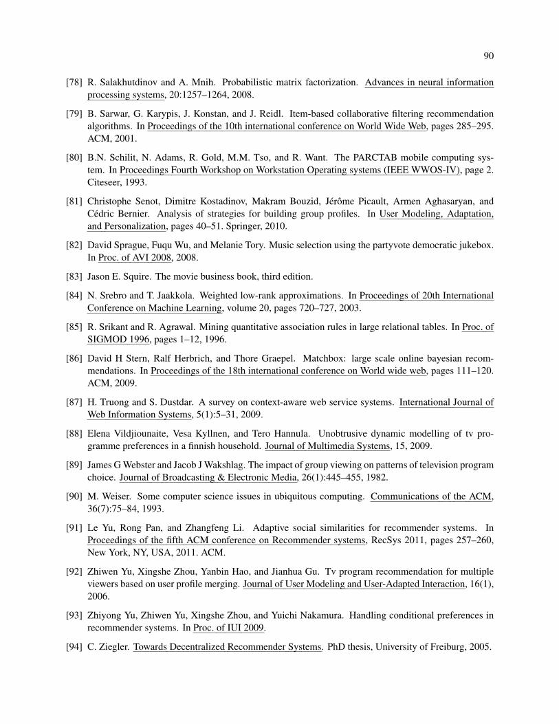
90
[78] R. Salakhutdinov and A. Mnih. Probabilistic matrix factorization. Advances in neural information
processing systems, 20:1257–1264, 2008.
[79] B. Sarwar, G. Karypis, J. Konstan, and J. Reidl. Item-based collaborative filtering recommendation
algorithms. In Proceedings of the 10th international conference on World Wide Web, pages 285–295.
ACM, 2001.
[80] B.N. Schilit, N. Adams, R. Gold, M.M. Tso, and R. Want. The PARCTAB mobile computing sys-
tem. In Proceedings Fourth Workshop on Workstation Operating systems (IEEE WWOS-IV), page 2.
Citeseer, 1993.
[81] Christophe Senot, Dimitre Kostadinov, Makram Bouzid, Jerome Picault, Armen Aghasaryan, and
Cedric Bernier. Analysis of strategies for building group profiles. In User Modeling, Adaptation,
and Personalization, pages 40–51. Springer, 2010.
[82] David Sprague, Fuqu Wu, and Melanie Tory. Music selection using the partyvote democratic jukebox.
In Proc. of AVI 2008, 2008.
[83] Jason E. Squire. The movie business book, third edition.
[84] N. Srebro and T. Jaakkola. Weighted low-rank approximations. In Proceedings of 20th International
Conference on Machine Learning, volume 20, pages 720–727, 2003.
[85] R. Srikant and R. Agrawal. Mining quantitative association rules in large relational tables. In Proc. of
SIGMOD 1996, pages 1–12, 1996.
[86] David H Stern, Ralf Herbrich, and Thore Graepel. Matchbox: large scale online bayesian recom-
mendations. In Proceedings of the 18th international conference on World wide web, pages 111–120.
ACM, 2009.
[87] H. Truong and S. Dustdar. A survey on context-aware web service systems. International Journal of
Web Information Systems, 5(1):5–31, 2009.
[88] Elena Vildjiounaite, Vesa Kyllnen, and Tero Hannula. Unobtrusive dynamic modelling of tv pro-
gramme preferences in a finnish household. Journal of Multimedia Systems, 15, 2009.
[89] James G Webster and Jacob J Wakshlag. The impact of group viewing on patterns of television program
choice. Journal of Broadcasting & Electronic Media, 26(1):445–455, 1982.
[90] M. Weiser. Some computer science issues in ubiquitous computing. Communications of the ACM,
36(7):75–84, 1993.
[91] Le Yu, Rong Pan, and Zhangfeng Li. Adaptive social similarities for recommender systems. In
Proceedings of the fifth ACM conference on Recommender systems, RecSys 2011, pages 257–260,
New York, NY, USA, 2011. ACM.
[92] Zhiwen Yu, Xingshe Zhou, Yanbin Hao, and Jianhua Gu. Tv program recommendation for multiple
viewers based on user profile merging. Journal of User Modeling and User-Adapted Interaction, 16(1),
2006.
[93] Zhiyong Yu, Zhiwen Yu, Xingshe Zhou, and Yuichi Nakamura. Handling conditional preferences in
recommender systems. In Proc. of IUI 2009.
[94] C. Ziegler. Towards Decentralized Recommender Systems. PhD thesis, University of Freiburg, 2005.
Recommended


![A Fuzzy Recommender System for eElections - unifr.ch Fuzzy Recommender System for eElections 63 2 Recommender Systems for eCommerce According to Yager [4], recommender systems used](https://img.pdfslide.net/doc/110x75/5b08be647f8b9a93738cdc60/a-fuzzy-recommender-system-for-eelections-unifrch-fuzzy-recommender-system-for.jpg)