Entropy, Relative Entropy, and Mutual InformationSome basic notions of Information Theory
Radu Trîmbitas
UBB
October 2012
Radu Trîmbitas (UBB) Entropy, Relative Entropy, and Mutual Information October 2012 1 / 66
Outline
1 Entropy and its PropertiesEntropyJoint Entropy and Conditional EntropyRelative Entropy and Mutual InformationRelationship between Entropy and Mutual InformationChain Rules for Entropy, Relative Entropy and Mutual information
2 Inequalities in Information TheoryJensen inequality and its consequencesLog sum inequality and its applicationsData-processing inequalitySu¢ cient statisticsFano�s inequality
Radu Trîmbitas (UBB) Entropy, Relative Entropy, and Mutual Information October 2012 2 / 66
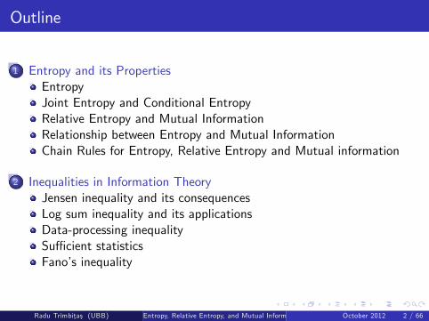
Entropy of a discrete RV
a measure of uncertainty of a random variableX a discrete random variable
X ��xipi
�i2I, X alphabet of X , p(x) = P(X = x), mass function of X
De�nition 1
The entropy of the discrete random variable X
H(X ) = � ∑x2X
p(x) log p(x) (1)
H(X ) = Ep
�log
1p(x)
�equivalent expression (2)
measured in bits!base 2! Hb(X ) entropy in base b; for b = e, measured in nats!convention 0 log 0 = 0, since limx&0 x log x = 0Radu Trîmbitas (UBB) Entropy, Relative Entropy, and Mutual Information October 2012 3 / 66
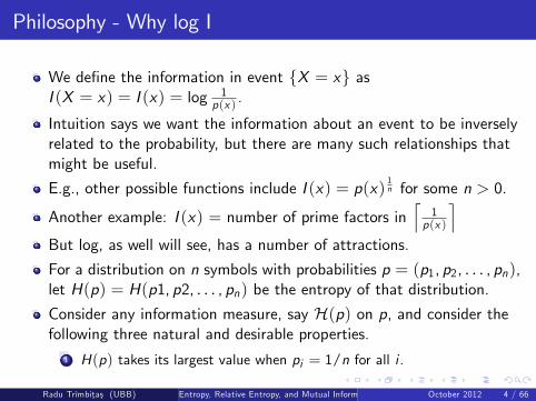
Philosophy - Why log I
We de�ne the information in event fX = xg asI (X = x) = I (x) = log 1
p(x ) .
Intuition says we want the information about an event to be inverselyrelated to the probability, but there are many such relationships thatmight be useful.
E.g., other possible functions include I (x) = p(x)1n for some n > 0.
Another example: I (x) = number of prime factors inl
1p(x )
mBut log, as well will see, has a number of attractions.
For a distribution on n symbols with probabilities p = (p1, p2, . . . , pn),let H(p) = H(p1, p2, . . . , pn) be the entropy of that distribution.Consider any information measure, say H(p) on p, and consider thefollowing three natural and desirable properties.
1 H(p) takes its largest value when pi = 1/n for all i .
Radu Trîmbitas (UBB) Entropy, Relative Entropy, and Mutual Information October 2012 4 / 66
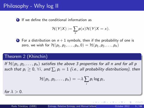
Philosophy - Why log II
2 If we de�ne the conditional information as
H(Y jX ) := ∑xp(x)H(Y jX = x).
3 For a distribution on n+ 1 symbols, then if the probability of one iszero, we wish for H(p1, p2, . . . , pn , 0) = H(p1, p2, . . . , pn)
Theorem 2 (Khinchin)
If H(p1, p2, . . . , pn) satis�es the above 3 properties for all n and for all psuch that pi � 0, 8i , and ∑i pi = 1 (i.e., all probability distributions), then
H(p1, p2, . . . , pn) = �λ ∑ipi log pi ,
for λ > 0.
Radu Trîmbitas (UBB) Entropy, Relative Entropy, and Mutual Information October 2012 5 / 66

Philosophy - Why log III
Theorem 3If a sequence of symmetric function Hm(p1, p2, . . . , pm) satis�es
1 Normalization H2� 12 ,12
�= 1,
2 Continuity: H2(p, 1� p) is a continuous function on p3 Grouping: Hm(p1, p2, . . . , pm) =Hm�1(p1 + p2, p3, . . . , pm) + (p1 + p2)H2
�p1
p1+p2, p1p1+p2
�,
then Hm must be of the form
Hm(p1, p2, . . . , pm) = �m
∑i=1pi log pi , m = 2, 3, . . .
Radu Trîmbitas (UBB) Entropy, Relative Entropy, and Mutual Information October 2012 6 / 66
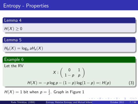
Entropy - Properties
Lemma 4
H(X ) � 0
Lemma 5
Hb(X ) = logb aHa(X )
Example 6Let the RV
X :�
0 11� p p
�H(X ) = �p log p � (1� p) log(1� p) =: H(p) (3)
H(X ) = 1 bit when p = 12 . Graph in Figure 1
Radu Trîmbitas (UBB) Entropy, Relative Entropy, and Mutual Information October 2012 7 / 66

Entropy - Properties II
Figure: Graph of H(p)
Radu Trîmbitas (UBB) Entropy, Relative Entropy, and Mutual Information October 2012 8 / 66
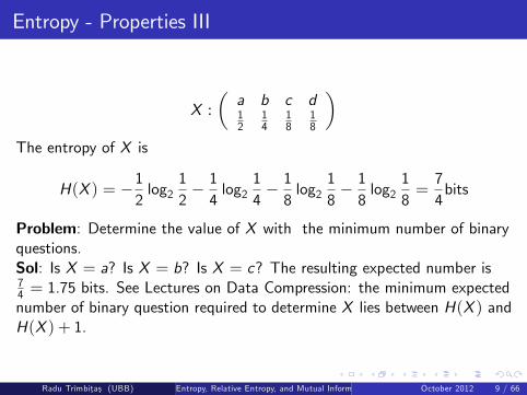
Entropy - Properties III
X :�a b c d12
14
18
18
�The entropy of X is
H(X ) = �12log2
12� 14log2
14� 18log2
18� 18log2
18=74bits
Problem: Determine the value of X with the minimum number of binaryquestions.Sol: Is X = a? Is X = b? Is X = c? The resulting expected number is74 = 1.75 bits. See Lectures on Data Compression: the minimum expectednumber of binary question required to determine X lies between H(X ) andH(X ) + 1.
Radu Trîmbitas (UBB) Entropy, Relative Entropy, and Mutual Information October 2012 9 / 66

Joint Entropy and Conditional Entropy I
(X ,Y ) a pair of discrete RVs over the alphabets X ,Y
X :�xipi
�i2I, Y :
�yjqj
�j2J
joint distribution of X and Y
p(x , y) = P(X = x ,Y = y), x 2 X , y 2 Y
(marginal) distribution of X
pX (x) = p(x) = P(X = x) = ∑y2Y
p(x , y)
(marginal) distribution of Y
pY (y) = p(y) = P(Y = y) = ∑x2X
p(x , y)
Radu Trîmbitas (UBB) Entropy, Relative Entropy, and Mutual Information October 2012 10 / 66

Joint Entropy and Conditional Entropy II
De�nition 7The joint entropy H(X ,Y ) of a pair of DRV (X ,Y ) � p(x , y)
H(X ,Y ) = � ∑x2X
∑y2Y
p(x , y) log p(x , y) (4)
also expressed as H(X ,Y ) = �E (log p(X ,Y ))
Radu Trîmbitas (UBB) Entropy, Relative Entropy, and Mutual Information October 2012 11 / 66
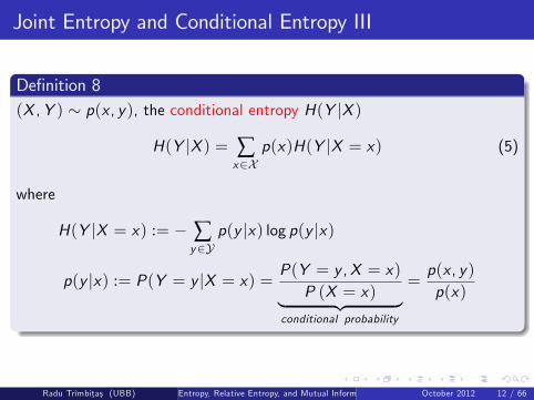
Joint Entropy and Conditional Entropy III
De�nition 8(X ,Y ) � p(x , y), the conditional entropy H(Y jX )
H(Y jX ) = ∑x2X
p(x)H(Y jX = x) (5)
where
H(Y jX = x) := � ∑y2Y
p(y jx) log p(y jx)
p(y jx) := P(Y = y jX = x) = P(Y = y ,X = x)P (X = x)| {z }
conditional probability
=p(x , y)p(x)
Radu Trîmbitas (UBB) Entropy, Relative Entropy, and Mutual Information October 2012 12 / 66
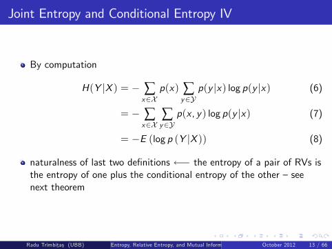
Joint Entropy and Conditional Entropy IV
By computation
H(Y jX ) = � ∑x2X
p(x) ∑y2Y
p(y jx) log p(y jx) (6)
= � ∑x2X
∑y2Y
p(x , y) log p(y jx) (7)
= �E (log p (Y jX )) (8)
naturalness of last two de�nitions � the entropy of a pair of RVs isthe entropy of one plus the conditional entropy of the other � seenext theorem
Radu Trîmbitas (UBB) Entropy, Relative Entropy, and Mutual Information October 2012 13 / 66

Joint Entropy and Conditional Entropy V
Theorem 9 (Chain Rule)
H(X ,Y ) = H(X ) +H(Y jX ). (9)
Radu Trîmbitas (UBB) Entropy, Relative Entropy, and Mutual Information October 2012 14 / 66

Joint Entropy and Conditional Entropy VI
Proof.
H(X ,Y ) = � ∑x2X
∑y2Y
p(x , y) log p(x , y)
= � ∑x2X
∑y2Y
p(x , y) log p(x)p(y jx)
= � ∑x2X
∑y2Y
p(x , y) log p(x)� ∑x2X
∑y2Y
p(x , y)p(y jx)
= � ∑x2X
p(x) log p(x)� ∑x2X
∑y2Y
p(x , y)p(y jx)
= H(X ) +H(Y jX ).
Equivalently (shorter proof): we can write
log p(X ,Y ) = log p(X ) + log p(Y jX )
and apply E to both sides.Radu Trîmbitas (UBB) Entropy, Relative Entropy, and Mutual Information October 2012 15 / 66

Joint Entropy and Conditional Entropy - b I
Corollary 10
H(X ,Y jZ ) = H(X jZ ) +H(Y jZ ,X ).
Example 11
Let (X ,Y ) have the joint distributionY nX 1 2 3 41 1
8116
132
132
2 116
18
132
132
3 116
116
116
116
4 14 0 0 0
marginal distributions X :� 12
14
18
18
�; Y :
� 14
14
14
14
�H(X ) = 7
4bits, H(Y ) = 2bits
Radu Trîmbitas (UBB) Entropy, Relative Entropy, and Mutual Information October 2012 16 / 66

Joint Entropy and Conditional Entropy - b II
conditional entropy
H(X jY ) =4
∑i=1p (Y = i)H (X jY = i)
=14H�12,14,18,18
�+14H�12,14,18,18
�+14H�14,14,14,14
�+14H (1, 0, 0, 0)
=14��74+74+ 2+ 0
�=118bits
H(Y jX ) = 138 bits and H(X ,Y ) =
278 bits.
Remark. If H(X ) 6= H(Y ) then H(Y jX ) 6= H(X jY ). HoweverH(X )�H(X jY ) = H(Y )�H(Y jX ).
Radu Trîmbitas (UBB) Entropy, Relative Entropy, and Mutual Information October 2012 17 / 66

Relative Entropy and Mutual Information I
De�nition 12The relative entropy or Kullback-Leibler distance between p(x) and q(x)
D (p k q) = ∑x2X
p(x) logp(x)q(x)
= Ep
�log
p(x)q(x)
�.
Conventions: 0 log 00 = 0, 0 log0q = 0, p log
p0 = ∞
It is not a true distance, since it is not symmetric and does not satisfythe triangle inequality � sometimes called Kullback-Leibler divergence.
Interpretation: The relative entropy is a measure of the distancebetween two distributions.
In statistics, it arises as an expected logarithm of the likelihood ratio.
Radu Trîmbitas (UBB) Entropy, Relative Entropy, and Mutual Information October 2012 18 / 66

Relative Entropy and Mutual Information II
The relative entropy D(p k q) is a measure of the ine¢ ciency ofassuming that the distribution is q when the true distribution is p. Forexample, if we knew the true distribution p of the random variable,we could construct a code with average description length H(p).
If, instead, we used the code for a distribution q, we would needH(p) +D(p k q) bits on the average to describe the random variable.
Radu Trîmbitas (UBB) Entropy, Relative Entropy, and Mutual Information October 2012 19 / 66

Relative Entropy and Mutual Information III
De�nition 13(X ,Y ) � p(x , y), p(x), p(y) mass functions; the mutual informationI (X ;Y ) is the relative entropy between p(x , y) and p(x)p(y) :
I (X ;Y ) = D (p(x , y) k p(x)p(y)) (10)
= ∑x2X
∑y2Y
p(x , y) logp(x , y)p(x)p(y)
(11)
= Ep(x ,y )
�log
p(X ,Y )p(X )p(Y )
�. (12)
Remark. D(p k q) 6= D(q k p), as the next example shown.Interpretation. I (X ;Y ) measures the average reduction in uncertainty of
X that results from knowing Y .
Radu Trîmbitas (UBB) Entropy, Relative Entropy, and Mutual Information October 2012 20 / 66

Relative Entropy and Mutual Information IV
Example 14
X = f0, 1g, p(0) = 1� r , p(1) = r , q(0) = 1� s, q(1) = s.
D(p k q) = (1� r) log 1� r1� s + r log
rs
D(q k p) = (1� s) log 1� s1� r + s log
sr
If r = s, then D(p k q) = D(q k p), but for r = 12 , s =
14
D(p k q) = 12log
1234
+12log
1214
= 0.207 52 bit
D(q k p) = 34log
3412
+14log
1412
= 0.188 72 bit
Radu Trîmbitas (UBB) Entropy, Relative Entropy, and Mutual Information October 2012 21 / 66
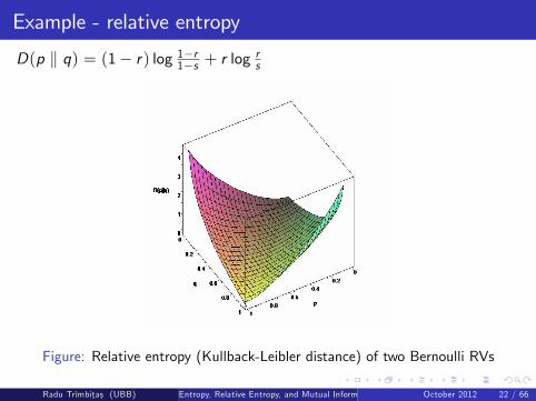
Example - relative entropy
D(p k q) = (1� r) log 1�r1�s + r logrs
Figure: Relative entropy (Kullback-Leibler distance) of two Bernoulli RVs
Radu Trîmbitas (UBB) Entropy, Relative Entropy, and Mutual Information October 2012 22 / 66

Relationship between Entropy and Mutual Information I
Theorem 15 (Mutual information and entropy)
I (X ;Y ) = H(X )�H(Y jX ) (13)
I (X ;Y ) = H(Y )�H(X jY ) (14)
I (X ;Y ) = H(X ) +H(Y )�H(X ,Y ) (15)
I (X ;Y ) = I (Y ,X ) (16)
I (X ,X ) = H(X ) (17)
Radu Trîmbitas (UBB) Entropy, Relative Entropy, and Mutual Information October 2012 23 / 66

Relationship between Entropy and Mutual Information II
Proof.(13)
I (X ;Y ) = ∑x2X
∑y2Y
p(x , y) logp(x , y)p(x)p(y)
= ∑x2X
∑y2Y
p(x , y) logp(x jy)p(x)
= � ∑x2X
∑y2Y
p(x , y)| {z }p(x )
log p(x) + ∑x2X
∑y2Y
p(x , y) log p(x jy)
= H(X )� � ∑x2X
∑y2Y
p(x , y) log p(x jy)!
= H(X )�H(X jY )
(14) by symmetry(15) results from (13) and H(X ,Y ) = H(Y )�H(X jY ); (15)=)(16)Finally, I (X ;X ) = H(X )�H(X jX ) = H(X ).
Radu Trîmbitas (UBB) Entropy, Relative Entropy, and Mutual Information October 2012 24 / 66
Relationship between entropy and mutual information
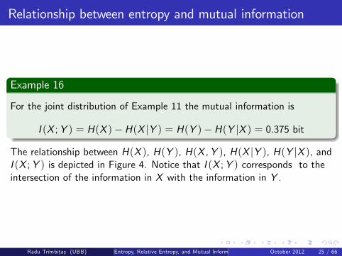
Example 16
For the joint distribution of Example 11 the mutual information is
I (X ;Y ) = H(X )�H(X jY ) = H(Y )�H(Y jX ) = 0.375 bit
The relationship between H(X ), H(Y ), H(X ,Y ), H(X jY ), H(Y jX ), andI (X ;Y ) is depicted in Figure 4. Notice that I (X ;Y ) corresponds to theintersection of the information in X with the information in Y .
Radu Trîmbitas (UBB) Entropy, Relative Entropy, and Mutual Information October 2012 25 / 66

Relationship between entropy and mutual information
Figure: Graphical representation of the relation between entropy and mutualinformation
Radu Trîmbitas (UBB) Entropy, Relative Entropy, and Mutual Information October 2012 26 / 66

Relationship between entropy and mutual information -graphical
Figure: Venn diagram for the relationship between entropy and mutualinformation
Radu Trîmbitas (UBB) Entropy, Relative Entropy, and Mutual Information October 2012 27 / 66
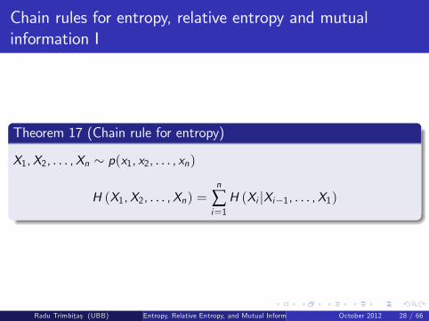
Chain rules for entropy, relative entropy and mutualinformation I
Theorem 17 (Chain rule for entropy)
X1,X2, . . . ,Xn � p(x1, x2, . . . , xn)
H (X1,X2, . . . ,Xn) =n
∑i=1H (Xi jXi�1, . . . ,X1)
Radu Trîmbitas (UBB) Entropy, Relative Entropy, and Mutual Information October 2012 28 / 66

Chain rules for entropy, relative entropy and mutualinformation II
Proof.Apply repeatedly the two variable expansion rule for entropy
H(X1,X2) = H(X1) +H(X2jX1),H(X1,X2,X3) = H(X1) +H(X2,X3jX1)
= H(X1) +H(X2jX1) +H(X3jX2,X1)...
H (X1,X2, . . . ,Xn) = H(X1) +H(X2jX1) + � � �+H (Xn jXn�1, . . . ,X1)
=n
∑i=1H (Xi jXi�1, . . . ,X1) .
Radu Trîmbitas (UBB) Entropy, Relative Entropy, and Mutual Information October 2012 29 / 66
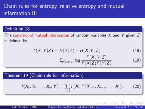
Chain rules for entropy, relative entropy and mutualinformation III
De�nition 18The conditional mutual information of random variables X and Y given Zis de�ned by
I (X ;Y jZ ) = H(X jZ )�H(X jY ,Z ) (18)
= Ep(x ,y ,z ) logP(X ,Y jZ )
P(X jZ )P(Y jZ ) (19)
Theorem 19 (Chain rule for information)
I (X1,X2, . . . ,Xn;Y ) =n
∑i=1I (Xi ;Y jXi�1,Xi�2, . . . ,X1) . (20)
Radu Trîmbitas (UBB) Entropy, Relative Entropy, and Mutual Information October 2012 30 / 66
Chain rules for entropy, relative entropy and mutualinformation IV
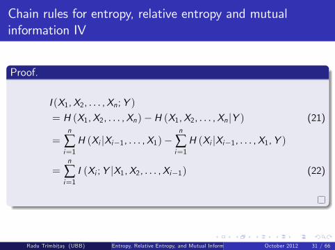
Proof.
I (X1,X2, . . . ,Xn;Y )= H (X1,X2, . . . ,Xn)�H (X1,X2, . . . ,Xn jY ) (21)
=n
∑i=1H (Xi jXi�1, . . . ,X1)�
n
∑i=1H (Xi jXi�1, . . . ,X1,Y )
=n
∑i=1I (Xi ;Y jX1,X2, . . . ,Xi�1) (22)
Radu Trîmbitas (UBB) Entropy, Relative Entropy, and Mutual Information October 2012 31 / 66

Chain rules for entropy, relative entropy and mutualinformation V
De�nition 20For joint probability mass functions p(x , y) and q(x , y), the conditionalrelative entropy is
D (p(x , y) k q(x , y)) = ∑xp(x)∑
yp(y jx) log p(y jx)
q(y jx) (23)
= Ep(x ,y ) logp (Y jX )q (Y jX ) . (24)
The notation is not explicit since it omits the mention of the distributionp(x) of the conditioning RV. However it is normally understood from thecontext.
Radu Trîmbitas (UBB) Entropy, Relative Entropy, and Mutual Information October 2012 32 / 66
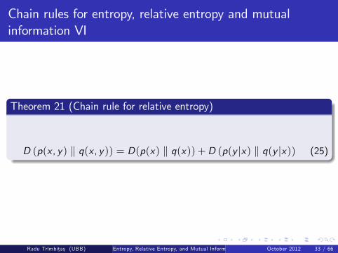
Chain rules for entropy, relative entropy and mutualinformation VI
Theorem 21 (Chain rule for relative entropy)
D (p(x , y) k q(x , y)) = D(p(x) k q(x)) +D (p(y jx) k q(y jx)) (25)
Radu Trîmbitas (UBB) Entropy, Relative Entropy, and Mutual Information October 2012 33 / 66

Chain rules for entropy, relative entropy and mutualinformation VII
Proof.
D(p(x , y)jjq(x , y))
= ∑x
∑yp(x , y) log
p(x , y)q(x , y)
= ∑x
∑yp(x , y) log
p(x)p(y jx)q(x)q(y jx)
= ∑x
∑yp(x , y) log
p(x)q(x)
+∑x
∑yp(x , y) log
p(y jx)q(y jx)
= D(p(x) k q(x)) +D (p(y jx) k q(y jx)) .
Radu Trîmbitas (UBB) Entropy, Relative Entropy, and Mutual Information October 2012 34 / 66

Jensen inequality I
Convexity underlies many of the basic properties of information-theoreticquantities such as entropy and mutual information.
De�nitions 221 A function f (x) is convex[ over an interval (a, b) if for everyx1, x2 2 (a, b) and 0 � λ � 1
f (λx1 + (1� λ) x2) � λf (x1) + (1� λ)f (x2). (26)
2 f is strictly convex if equality holds only for λ = 0 and λ = 1.3 f is concave\ if �f is convex.
A function is convex if it always lies below any chord. A function isconcave if it always lies above any chord.
Examples of convex functions: x2, jx j, ex , x log x for x � 0.
Radu Trîmbitas (UBB) Entropy, Relative Entropy, and Mutual Information October 2012 35 / 66
Jensen inequality II
Example of concave functions: log x andpx for x � 0.
If f 00 nonnegative (positive) then f is convex (strictly convex)
Theorem 23 (Jensen�s inequality)
If f is a convex function and X is a RV
E (f (X )) � f (E (X )). (27)
If f is strictly convex, equality in (27) implies X = E (X ) with probability1 (i.e. X is a constant).
Radu Trîmbitas (UBB) Entropy, Relative Entropy, and Mutual Information October 2012 36 / 66

Jensen inequality III
Proof.for discrete RV induction on number of mass points.For a two-mass-point distribution, we apply the de�nition
f (p1x1 + p2x2) � p1f (x1) + p2f (x2)
Suppose true for k � 1; we set p0i = pi/ (1� pk )
f
k
∑i=1pixi
!= f
pkxk + (1� pk )
k�1∑i=1
p0ixi
!
� pk f (xk ) + (1� pk )f k�1∑i=1
p0ixi
!
� pk f (xk ) + (1� pk )k�1∑i=1
p0i f (xi ) =k
∑i=1pi f (xi ) .
Extension to continuous distributions using continuity arguments.Radu Trîmbitas (UBB) Entropy, Relative Entropy, and Mutual Information October 2012 37 / 66
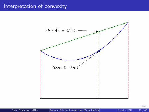
Interpretation of convexity
Radu Trîmbitas (UBB) Entropy, Relative Entropy, and Mutual Information October 2012 38 / 66
Consequences of Jensen Inequality I
We will use Jensen to prove properties of entropy and relative entropy.
Theorem 24 (Information inequality, Gibbs�inequality)
p(x), q(x), x 2 X pmfD (p k q) � 0 (28)
with equality i¤ p(x) = q(x), 8x 2 X .
Radu Trîmbitas (UBB) Entropy, Relative Entropy, and Mutual Information October 2012 39 / 66
Consequences of Jensen Inequality II
Proof.Let A := fx : p(x) > 0g
D (p k q) = ∑x2A
p(x) logp(x)q(x)
= ∑x2A
p(x)�� log q(x)
p(x)
�
� � log
∑x2A
p(x)q(x)p(x)
!(- log is strictly convex)
= � log ∑x2A
q(x) = � log 1 = 0
Equality hold i¤ q(x )p(x ) = c , 8x 2 X . But, 1 = ∑x2A q(x) = ∑x2X q(x)
= c ∑x2X p(x) = c , so p(x) = q(x), 8x 2 X .
Since I (X ,Y ) = D(p(x , y) k p(x)q(x)) � 0, with equality i¤p(x , y) = p(x)q(x) (i.e. X and Y are independent) we obtain
Radu Trîmbitas (UBB) Entropy, Relative Entropy, and Mutual Information October 2012 40 / 66
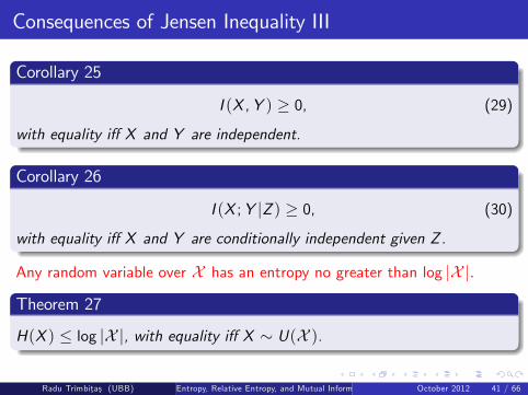
Consequences of Jensen Inequality III
Corollary 25
I (X ,Y ) � 0, (29)
with equality i¤ X and Y are independent.
Corollary 26
I (X ;Y jZ ) � 0, (30)
with equality i¤ X and Y are conditionally independent given Z.
Any random variable over X has an entropy no greater than log jX j.
Theorem 27
H(X ) � log jX j, with equality i¤ X � U(X ).
Radu Trîmbitas (UBB) Entropy, Relative Entropy, and Mutual Information October 2012 41 / 66

Consequences of Jensen Inequality IV
Proof.
p(x) pmf of X , u(x) = 1jX j pmf of uniform distribution over X .
0 � D(p k u) = ∑x2X
p(x) logp(x)u(x)
= log jX j �H(X ).
The next theorem states that conditioning reduces entropy (orinformation cannot hurt).
Theorem 28
H(X jY ) � H(X )with equality i¤ X and Y are independent.
Radu Trîmbitas (UBB) Entropy, Relative Entropy, and Mutual Information October 2012 42 / 66

Consequences of Jensen Inequality V
Proof.0 � I (X ,Y ) = H(X )�H(X jY ).
Corollary 29 (Independence bound on entropy)
H(X1,X2, . . . ,X ) �n
∑i=1H(Xi )
Radu Trîmbitas (UBB) Entropy, Relative Entropy, and Mutual Information October 2012 43 / 66

Consequences of Jensen Inequality VI
Proof.Chain rule for entropy (Theorem 17)
H(X1,X2, . . . ,X ) =n
∑i=1H(Xi jXi�1, . . . ,X1) � H(Xi ) ( � from Th. 28)
Radu Trîmbitas (UBB) Entropy, Relative Entropy, and Mutual Information October 2012 44 / 66
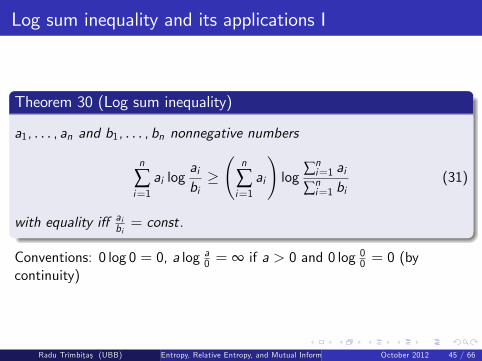
Log sum inequality and its applications I
Theorem 30 (Log sum inequality)
a1, . . . , an and b1, . . . , bn nonnegative numbers
n
∑i=1ai log
aibi�
n
∑i=1ai
!log
∑ni=1 ai
∑ni=1 bi
(31)
with equality i¤ aibi= const.
Conventions: 0 log 0 = 0, a log a0 = ∞ if a > 0 and 0 log 00 = 0 (bycontinuity)
Radu Trîmbitas (UBB) Entropy, Relative Entropy, and Mutual Information October 2012 45 / 66

Log sum inequality and its applications II
Proof.Assume w.l.o.g. ai > 0, bi > 0. Since f (t) = t log t is convex for t > 0,by Jensen ineq.
∑ αi f (ti ) � f�∑ αi ti
�, αi � 0,∑ αi = 1.
Setting αi =bi
∑ bjand ti =
aibi, we obtain
∑ai
∑ bjlog
aibi�∑
ai∑ bj
log∑ai
∑ bj,
the desired inequality.
Homework. Prove Theorem 24 using log sum inequality.Using log sum inequality it is easy to prove convexity and concavity resultsfor relative entropy, entropy and mutual information. See [1, Section 2.7].
Radu Trîmbitas (UBB) Entropy, Relative Entropy, and Mutual Information October 2012 46 / 66
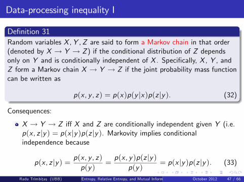
Data-processing inequality I
De�nition 31Random variables X ,Y ,Z are said to form a Markov chain in that order(denoted by X ! Y ! Z ) if the conditional distribution of Z dependsonly on Y and is conditionally independent of X . Speci�cally, X , Y , andZ form a Markov chain X ! Y ! Z if the joint probability mass functioncan be written as
p(x , y , z) = p(x)p(y jx)p(z jy). (32)
Consequences:
X ! Y ! Z i¤ X and Z are conditionally independent given Y (i.e.p(x , z jy) = p(x jy)p(z jy). Markovity implies conditionalindependence because
p(x , z jy) = p(x , y , z)p(y)
=p(x , y)p(z jy)
p(y)= p(x jy)p(z jy). (33)
Radu Trîmbitas (UBB) Entropy, Relative Entropy, and Mutual Information October 2012 47 / 66

Data-processing inequality II
X ! Y ! Z =) Z ! Y ! X , sometimes written asX ! Y ! Z . (reversibility)
If Z = f (Y ), then X ! Y ! Z
We will prove that no processing of Y , deterministic or random, canincrease the information that Y contains about X .
Theorem 32 (Data-processing inequality)
If X ! Y ! Z, then I (X ;Y ) � I (X ;Z ).
Radu Trîmbitas (UBB) Entropy, Relative Entropy, and Mutual Information October 2012 48 / 66
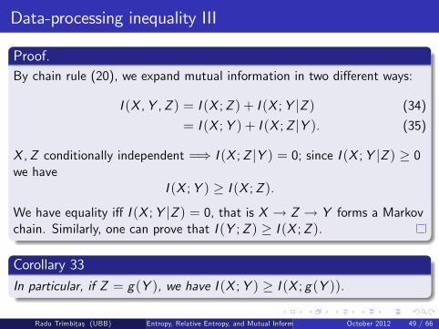
Data-processing inequality III
Proof.By chain rule (20), we expand mutual information in two di¤erent ways:
I (X ,Y ,Z ) = I (X ;Z ) + I (X ;Y jZ ) (34)
= I (X ;Y ) + I (X ;Z jY ). (35)
X ,Z conditionally independent =) I (X ;Z jY ) = 0; since I (X ;Y jZ ) � 0we have
I (X ;Y ) � I (X ;Z ).We have equality i¤ I (X ;Y jZ ) = 0, that is X ! Z ! Y forms a Markovchain. Similarly, one can prove that I (Y ;Z ) � I (X ;Z ).
Corollary 33
In particular, if Z = g(Y ), we have I (X ;Y ) � I (X ; g(Y )).
Radu Trîmbitas (UBB) Entropy, Relative Entropy, and Mutual Information October 2012 49 / 66
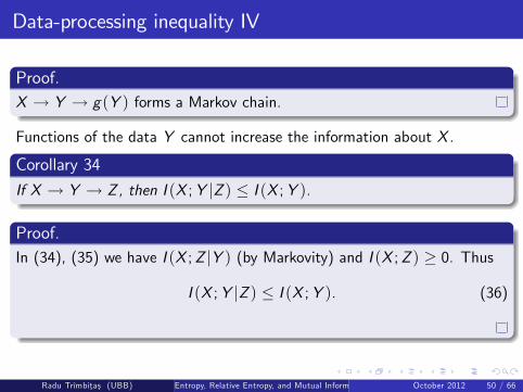
Data-processing inequality IV
Proof.X ! Y ! g(Y ) forms a Markov chain.
Functions of the data Y cannot increase the information about X .
Corollary 34
If X ! Y ! Z, then I (X ;Y jZ ) � I (X ;Y ).
Proof.In (34), (35) we have I (X ;Z jY ) (by Markovity) and I (X ;Z ) � 0. Thus
I (X ;Y jZ ) � I (X ;Y ). (36)
Radu Trîmbitas (UBB) Entropy, Relative Entropy, and Mutual Information October 2012 50 / 66

Data-processing inequality V
If X ,Y ,Z do not form a Markov chain it is possible thatI (X ;Y jZ ) > I (X ;Y ). For example, if X and Y are independent fairbinary RVs and Z = X + Y , then I (X ;Y ) = 0,I (X ;Y jZ ) = H(X jZ )�H(X jY ,Z ) = H(X jZ ). But,H(X jZ ) = P(Z = 1)H(X jZ = 1) = 1
2 bit.
Radu Trîmbitas (UBB) Entropy, Relative Entropy, and Mutual Information October 2012 51 / 66

Su¢ cient statistics I
We apply data-processing inequality in statistics
ffθ(x)g family of pmfs, X � fθ(x), T (X ) statisticsθ ! X ! T (X ); data-processing inequality (Theorem 32) implies
I (θ;T (X )) � I (θ;X ) (37)
with equality when no information is lost.
A statistic T (X ) is called su¢ cient for θ if it contains all theinformation in X about θ.
Radu Trîmbitas (UBB) Entropy, Relative Entropy, and Mutual Information October 2012 52 / 66
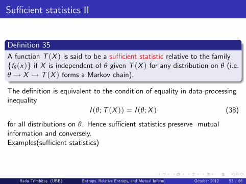
Su¢ cient statistics II
De�nition 35A function T (X ) is said to be a su¢ cient statistic relative to the familyffθ(x)g if X is independent of θ given T (X ) for any distribution on θ (i.e.θ ! X ! T (X ) forms a Markov chain).
The de�nition is equivalent to the condition of equality in data-processinginequality
I (θ;T (X )) = I (θ;X ) (38)
for all distributions on θ. Hence su¢ cient statistics preserve mutualinformation and conversely.Examples(su¢ cient statistics)
Radu Trîmbitas (UBB) Entropy, Relative Entropy, and Mutual Information October 2012 53 / 66

Su¢ cient statistics III
1 X1, X2, . . . , Xn, Xi 2 f0, 1g, a sequence of i.i.d. Bernoullian variableswith parameter θ = P(Xi = 1). Given n, the number of 1�s is asu¢ cient statistics for θ
T (X1, . . . ,Xn) =n
∑i=1Xi .
2 If X � N(θ, 1), that is
fθ(x) =1p2πe�
(x�θ)2
2
and X1, X2, . . . , Xn is a sample of i.i.d. N(θ, 1) RVs, thenX n = 1
n ∑ni=1 Xi is a su¢ cient statistic.
3 fθ(x) pdf for U(θ, θ + 1) - a su¢ cient statistic for θ is
T (X1, . . . ,Xn) = (minfXig,maxfXig) .Radu Trîmbitas (UBB) Entropy, Relative Entropy, and Mutual Information October 2012 54 / 66

Su¢ cient statistics IV
De�nition 36A statistic T (X ) is a minimal su¢ cient statistic relative to ffθ(x)g if it isa function of every other su¢ cient statistic U,
θ ! T (X )! U(X )! X .
Hence, a minimal su¢ cient statistic maximally compresses the informationabout θ in the sample.
Radu Trîmbitas (UBB) Entropy, Relative Entropy, and Mutual Information October 2012 55 / 66

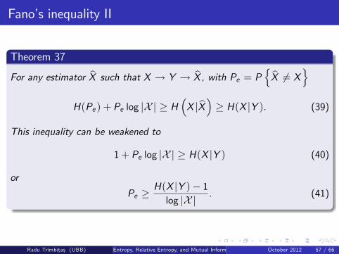
Fano�s inequality I
Suppose we wish to estimate X � p(x)We observe Y related to X by the conditional distribution p(y jx).From Y we calculate g(Y ) = bX ; bX is an estimate of X over thealphabet bX .X ! Y ! bX forms a Markov chain
De�ne the probability of error
Pe = PnbX 6= Xo .
Radu Trîmbitas (UBB) Entropy, Relative Entropy, and Mutual Information October 2012 56 / 66
Fano�s inequality II
Theorem 37
For any estimator bX such that X ! Y ! bX, with Pe = P nbX 6= XoH(Pe ) + Pe log jX j � H
�X jbX� � H(X jY ). (39)
This inequality can be weakened to
1+ Pe log jX j � H(X jY ) (40)
or
Pe �H(X jY )� 1log jX j . (41)
Radu Trîmbitas (UBB) Entropy, Relative Entropy, and Mutual Information October 2012 57 / 66
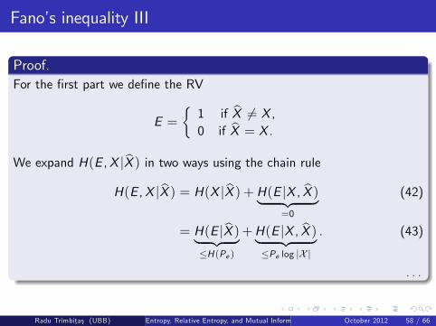
Fano�s inequality III
Proof.For the �rst part we de�ne the RV
E =�1 if bX 6= X ,0 if bX = X .
We expand H(E ,X jbX ) in two ways using the chain ruleH(E ,X jbX ) = H(X jbX ) +H(E jX , bX )| {z }
=0
(42)
= H(E jbX )| {z }�H (Pe )
+H(E jX , bX )| {z }�Pe log jX j
. (43)
. . .
Radu Trîmbitas (UBB) Entropy, Relative Entropy, and Mutual Information October 2012 58 / 66

Fano�s inequality IV
Proof - continuation.
Since E is a function of X and bX , H(E jX , bX ) = 0.H(E jbX ) � H(E ) = H(Pe ) (conditioning reduce entropy)Since for E = 0, bX = X and for E = 1 entropy is less than thenumber of possible outcomes
H(E jX , bX ) = P(E = 0)H(X jbX ,E = 0) + P(E = 1)H(X jbX ,E = 1)� (1� Pe ) � 0+ Pe log jX j (44)
. . .
Radu Trîmbitas (UBB) Entropy, Relative Entropy, and Mutual Information October 2012 59 / 66
Fano�s inequality -continuation I
Proof - continuation.Combining these results, we obtain
H(Pe ) + Pe log jX j � H(X jbX )X ! Y ! bX Markov chain=) I (X ; bX ) � I (X ;Y ) =) H(X jbX ) � H(X jY ).Finally,
H(Pe ) + Pe log jX j � H�X jbX� � H(X jY ).
Radu Trîmbitas (UBB) Entropy, Relative Entropy, and Mutual Information October 2012 60 / 66

Fano�s inequality - consequences I
If we set bX = Y in Fano�s inequality, we obtain
Corollary 38
For any two RVs X and Y , let p = P (X 6= Y ). Then
H(p) + p log jX j � H(X jY ). (45)
If the estimator g(Y ) takes values in X , we can replace log jX j bylog (jX j � 1).
Corollary 39
Let Pe = P(X 6= bX ), and let bX : Y ! X ; then
H(Pe ) + Pe log (jX j � 1) � H(X jY ).
Radu Trîmbitas (UBB) Entropy, Relative Entropy, and Mutual Information October 2012 61 / 66

Fano�s inequality - consequences II
Proof.Like the proof of Theorem 37, excepting that in (44), the range of possibleX outcomes has the cardinal jX j � 1.
Remark. Suppose there is no knowledge of Y . Thus, X must be guessedwithout any information. Let X 2 f1, 2, . . . ,mg and p1 � p2 � � � � � pm .Then the best guess of X is bX = 1 and the resulting probability error isPe = 1� p1. Fano�s inequality becomes
H(Pe ) + Pe log(m� 1) � H(X ).
The pmf
(p1, p2, . . . , pm) =�1� Pe ,
Pem� 1 , . . . ,
Pem� 1
�achieves this bound with equality: Fano�s inequality is sharp!
Radu Trîmbitas (UBB) Entropy, Relative Entropy, and Mutual Information October 2012 62 / 66
Fano�s inequality - consequences III
Next results relates probability of error and entropy. Let X and X 0 be i.i.d.RVs with entropy H(X ).
P(X = X 0) = ∑xp2(x).
Lemma 40
If X and X 0 are i.i.d. RVs with entropy H(X ),
P(X = X 0) � 2�H (x ), (46)
with equality i¤ X has uniform distribution.
Radu Trîmbitas (UBB) Entropy, Relative Entropy, and Mutual Information October 2012 63 / 66

Fano�s inequality - consequences IV
Proof.Suppose X � p(x); Jensen implies
2E (log p(X )) � E�2log P (X )
�2�H (X ) = 2∑ p(x ) log p(x ) �∑ p(x)2log p(x ) = ∑ p2(x).
Corollary 41
Let X~p(x), X 0 � r(x), independent RVs over X . Then
P(X = X 0) � 2�H (p)�D (pkr ) (47)
P(X = X 0) � 2�H (r )�D (rkp). (48)
Radu Trîmbitas (UBB) Entropy, Relative Entropy, and Mutual Information October 2012 64 / 66

Fano�s inequality - consequences V
Proof.
2�H (p)�D (pkr ) = 2∑ p(x ) log p(x )+∑ p(x ) log r (x )p(x )
= 2∑ p(x ) log r (x )
From Jensen and convexity of f (y) = 2y it follows
2�H (p)�D (pkr ) �∑ p(x)2log r (x )
= ∑ p(x)r(x) = P(X = X 0).
Radu Trîmbitas (UBB) Entropy, Relative Entropy, and Mutual Information October 2012 65 / 66

References
Thomas M. Cover, Joy A. Thomas, Elements of Information Theory,2nd edition, Wiley, 2006.
David J.C. MacKay, Information Theory, Inference, and LearningAlgorithms, Cambridge University Press, 2003.
Robert M. Gray, Entropy and Information Theory, Springer, 2009
Radu Trîmbitas (UBB) Entropy, Relative Entropy, and Mutual Information October 2012 66 / 66
Recommended


![Recoverability in quantum information theory · Mark M. Wilde (LSU) 2 / 23. Background | entropies Umegaki relative entropy [Ume62] The quantum relative entropy is a measure of dissimilarity](https://img.pdfslide.net/doc/110x75/5f30fba10d342e05863fbc67/recoverability-in-quantum-information-mark-m-wilde-lsu-2-23-background-entropies.jpg)