237
(3.154)
(3.153)
Lecture 16. SOLVING FOR TRANSIENT MOTIONUSING MODAL COORDINATES
Free MotionWith normalized eigenvectors, the matrix version of the modalEq.(3.125) is
= the modal force vector. Uncoupled, modal differential
equations:
The homogeneous version of Eq.(3.154)
have solutions:
238
Adding particular solutions corresponding to
specific right-hand forcing functions, yield the completesolution
The constants must be determined from the modal-
coordinate initial conditions.
To obtain modal-coordinate initial conditions:
Hence, the modal-coordinate initial conditions are defined by
Similarly, the modal-velocity initial conditions are defined by

239
(3.144)
(3.145)
(3.151)
For the prior example
with
Modal coordinate initial conditions:
240
(3.155b)
Modal velocity initial conditions:
With these initial conditions, we can solve Eqs.(3.132) for anyspecified modal force terms , obtaining a complete
modal-coordinate solution defined by . From
Eq.(3.123a) the solution for the physical coordinates can then bestated
Hence, the physical coordinate response vector is a linear sumof the modal solutions times their respective mode

241
(3.157)
shapes (or eigenvectors).
Example. With , Eqs. (3.155)
gives , and:
The corresponding physical-coordinate solution is
Any disturbance to the system from initial conditions (orexternal forces) will result in combined motion at the twonatural frequencies. Note that the physical initial conditions arecorrectly represented,
242
-1
-0.5
0
0.5
1
0 10 20 30 40
t
q_1
-1
-0.5
0
0.5
1
0 10 20 30 40
t
q_2
-2
-1
0
1
2
0 10 20 30 40
t
x_1
-1
-0.5
0
0.5
1
0 10 20 30 40
t
x_2
Figure 3.53 Solution from Eq.(3.157) for and for

243
( i )
Modal Transient Example Problem 1. Free UndampedMotion
The 2-mass model illustrated in a is just about to collide with awall. The right-hand spring will cushion the shock of thecollision. Before collision, the system’s model is
Once contact is established, the system looks like the model offrame b and is governed by the matrix differential equations ofmotion
244
( ii )
( ii )
The physical parameters are:
yielding
Starting from the instant of contact, the physical initialconditions are:
Solve for and the reaction forces
.

245
(iv)
Solution. Following the procedures of the preceding examples,the eigenvalues and natural frequencies are:
The matrix of unnormalized eigenvectors is
The matrix of normalized eigenvectors follows from as
Hence, the model is
From , the modal-coordinate initial
246
( v )
conditions are zero. From , the modal-
velocity initial conditions are
In terms of initial conditions, the solution to is
. Hence, the modal solutions
are:
From , the solution for the physical coordinates is

247
q_2 versus time
-1
-0.8-0.6
-0.4-0.2
0
0.20.4
0.60.8
1
0 0.1 0.2 0.3 0.4 0.5 0.6
t (seconds)
q_2
q_1 versus time
-2
0
2
4
6
8
10
0 0.1 0.2 0.3 0.4 0.5 0.6
t (seconds)
q_1
248
x_1 (m) versus time
-0.2
-0.10
0.10.2
0.3
0.40.5
0.60.7
0.8
0 0.1 0.2 0.3 0.4 0.5 0.6
t (seconds)
x_1
x_2 versus time
-0.1
-0.050
0.050.1
0.15
0.20.25
0.30.35
0.4
0 0.1 0.2 0.3 0.4 0.5 0.6
t (seconds)
x_2

249
f_s1=k_1 (x_1 - x_2 ) versus time
-1000
0
1000
2000
3000
4000
5000
6000
7000
0 0.1 0.2 0.3 0.4 0.5 0.6
t (seconds)
f_s1
= k
_1 (
x_1
- x_
2 )
(N)
f_s2 = k_2 x_2 versus time
-1000
0
1000
2000
3000
4000
5000
6000
0 0.1 0.2 0.3 0.4 0.5 0.6
time (seconds)
f_s2
= k
_2 x
_2 (
N)
250
Do the numbers seem right? We can do a quick calculation tosee if the peak force and deflection seem to be reasonable. Suppose both bodies are combined, so that one body has a massof . Then a conservation of
energy equation to find the peak deflection is
The predicted peak deflection for is 0.35 m , which is on
the order of magnitude for the estimate, but lower. We wouldexpect the correct number to be lower, because two masses witha spring between them will produce a lower collision force thana single rigid body with an equivalent mass.
Note that the spring-mass system loses contact with the wallwhen changes sign at about . After this
time, the right spring is disengaged, and the model becomes

251
(3.23)
(3.24)
(3.25)
Damping and Modal Damping FactorsThe SDOF harmonic oscillator equation of motion is
yields the homogeneous equation
Assumed solution: Yh=Aest yields:
Since A … 0, and ,
For ζ<1, the roots are
is called the damped natural frequency. The
homogeneous solution looks like
252
where A1 and A2 are complex coefficients. The solution can bestated
where A and B are real constants.
MDOF vibration problems with general damping matricesmodeled by,
also have complex roots (eigenvalues) and eigenvectors.
The matrix of real eigenvectors, based on a symmetric stiffness and mass matrices, will only diagonalize a damping
matrix that can be stated as a linear summation of and; i.e.,
For a damping matrix of this particular (and very unlikely)form, the modal damping matrix is defined by
253
where and are the identity matrix and the diagonalmatrix of eigenvectors, respectively. With this damping-matrixformat, an n-degree-of-freedom vibration problem will havemodal differential equations of the form:
This is not a very useful or generally applicable result. Forlightly damped systems, damping is more often introduceddirectly in the undamped modal equations via :
The damping factors are specified for each modal
differential equation, based on measurements or experience.
254
(3.129)
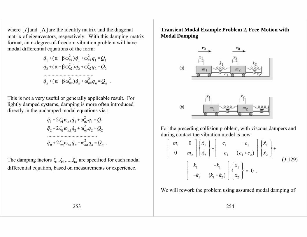
Transient Modal Example Problem 2, Free-Motion withModal Damping
For the preceding collision problem, with viscous dampers andduring contact the vibration model is now
We will rework the problem using assumed modal damping of

255
(3.27)
10% for each mode; i.e., . Hence
The modal differential equation model now looks like:
The solution to the differential equation is
For the initial conditions , the constants A,
B are solved from , and from
The solution is
256
Applying this result to the present example gives,
and the modal coordinate solutions are:
The transformation to obtain the physical coordinates remainsunchanged as

257
q_1 versus time
-1
0
1
2
3
4
5
6
7
8
9
0 0.1 0.2 0.3 0.4 0.5 0.6
t (seconds)
q_1
q_2 versus time
-0.8
-0.6
-0.4
-0.2
0
0.2
0.4
0.6
0 0.1 0.2 0.3 0.4 0.5 0.6
t (seconds)
q_2
258
x_1 (m) versus time
-0.1
0
0.1
0.2
0.3
0.4
0.5
0.6
0.7
0 0.1 0.2 0.3 0.4 0.5 0.6
t (seconds)
x_1
x_2 versus time
-0.05
0
0.05
0.1
0.15
0.2
0.25
0.3
0.35
0 0.1 0.2 0.3 0.4 0.5 0.6
t (seconds)
x_2

259
f_s1 = k_1 (x_1 - x_2) versus time
-1000
0
1000
2000
3000
4000
5000
0 0.1 0.2 0.3 0.4 0.5 0.6
t (seconds)
f_s1
= k
_1 (
x_1
- x
_2)
(N)
f_s2 = k_2 x_2 versus time
-1000
0
1000
2000
3000
4000
5000
6000
0 0.1 0.2 0.3 0.4 0.5 0.6
t (seconds)
f_s2
= k
_2 x
_2 (
N)
Adding damping reduces the peak force in spring 2 from 5363 N to
260
4820 N.
Recommended